


1. Introduction
Cavitation can generally be described by the process of liquid rupturing due to a drop in pressure at constant liquid temperature (Brennen Reference Brennen2014). As the pressure is lowered, by static or dynamic means, a state is reached where vapour (or gas)-filled bubbles (cavities) grow and become detectable. The rate of growth is nominal if the process is due to the diffusion of dissolved gas, or due to the expansion of gas as a result of a pressure drop. The rate of growth is explosive if it is primarily a result of vaporisation into the cavity. In its early stages, cavitation manifests from random molecular motions. In advanced stages beyond inception, it can manifest from more complex hydrodynamic events.
The events in the inception and development stages of cavitation depend on the condition of the liquid and on the pressure field in the zone of cavitation. Nuclei can be freely suspended (Yount, Gillary & Hoffman Reference Yount, Gillary and Hoffman1984); in this situation, if there are no impurities such as non-condensible gas, it is commonly referred to as homogeneous nucleation, and the tensions required to cause a rupture are greater than  $-60\,\mathrm {MPa}$ (Ando, Liu & Ohl Reference Ando, Liu and Ohl2012). On the other hand, heterogeneous nucleation occurs at pre-existing weaknesses, such as particles, or small pockets of gas in contact with solid boundaries such as container walls and particle surfaces (Andersen & Mørch Reference Andersen and Mørch2015), or other gaseous contaminants (Arora, Ohl & Mørch Reference Arora, Ohl and Mørch2004; Borkent, Arora & Ohl Reference Borkent, Arora and Ohl2007; Borkent et al. Reference Borkent, Arora, Ohl, De Jong, Versluis, Lohse, Mørch, Klaseboer and Khoo2008; Zhang et al. Reference Zhang, Belova, Wang, Dong and Möhwald2014). In engineering applications, cavitation occurs at pre-existing nuclei in the liquid, commonly observed at major weaknesses at the boundary between a solid and liquid (Greenspan & Tschiegg Reference Greenspan and Tschiegg1967; Caupin & Herbert Reference Caupin and Herbert2006). A detailed review on pre-existing gaseous nuclei can be found in Jones, Evans & Galvin (Reference Jones, Evans and Galvin1999).
The liquid can be either in motion or at rest, which is why cavitation is often observed in flowing streams, moving immersed bodies and under acoustic excitation. Typically, cavitation is characterised based on its appearance. Travelling cavitation is when individual transient nuclei form into bubbles in low-pressure regions, such as moving vortex cores that occur on the blade tips of ships’ propellers, or in turbulent shear flows where they expand and shrink in the liquid phase, and then collapse in higher-pressure regions. Fixed cavitation is typically associated with situations that develop after inception in which the liquid flow detaches from a solid boundary. If the cavity is attached then it is usually stable in a quasi-steady sense. Vibratory cavitation occurs due to high-amplitude, high-frequency pressure pulsations without any significant flow. This can occur near surfaces that vibrate, or due to ultrasonic excitation. Therefore, cavitation that occurs under dynamic pressure reduction, such as that under hydrodynamic and acoustic fields, causes a cyclical behaviour of bubble growth and collapse. Gas content plays a significant role in the sequence of events beginning with bubble formation and extending through bubble collapse. The incipient stage of cavitation is when cavities become barely detectable. The developed stage, which succeeds the incipient stage, is when cavities grow and vaporisation rates increase due to changes in velocity, pressure or temperature conditions. If the pressure is below some critical value for a certain period of time, then it will produce a cavitation event. This critical pressure is a characteristic of the physical properties of the system. The threshold between no cavitation and detectable cavitation is not always identical and is referred to as incipient and desinent cavitation events (Knapp, Dailey & Hammitt Reference Knapp, Dailey and Hammitt1970).
1.1. Nuclei in cavitation
Experimentally, detecting sub-micrometre particles in a liquid is difficult, making it challenging to distinguish between homogeneous and heterogeneous nucleation. Studies of the fundamental physics of the formation of vapour voids in the body of a pure liquid date back to Gibbs (Reference Gibbs1906), Volmer & Weber (Reference Volmer and Weber1926), Farkas (Reference Farkas1927), Becker & Döring (Reference Becker and Döring1935) and Zeldovich (Reference Zeldovich1943). A well-known approach is classical nucleation theory (CNT). Comprehensive reviews on CNT can be found in books by Frenkel (Reference Frenkel1955), Skripov (Reference Skripov1974) and Carey (Reference Carey2020) and in articles by Blake (Reference Blake1949a), Bernath (Reference Bernath1952), Cole (Reference Cole1974), Blander & Katz (Reference Blander and Katz1975) and Lienhard & Karimi (Reference Lienhard and Karimi1981). Recently, simulations using molecular dynamics have focused on modelling the inception and nucleation events (Menzl et al. Reference Menzl, Gonzalez, Geiger, Caupin, Abascal, Valeriani and Dellago2016; Chen et al. Reference Chen, Xue, Mahesh and Siepmann2019; Gao, Wu & Wang Reference Gao, Wu and Wang2021).
In this paper, we approach CNT from a general Gibbs free energy description with a focus on the behaviour and transition from homogeneous nucleation to heterogeneous nucleation in the presence of contaminant gas and the absence of a solid boundary. Vincent & Marmottant (Reference Vincent and Marmottant2017) investigate similar behaviour for confined bubbles within shells under static and dynamic conditions. The idea in this paper is to show that there is a smooth continuous behaviour between the two regimes. Expressions for the critical radius, activation energy and diameter of the initial bubble distribution are given by a set of analytic solutions. The transition between the two regimes is captured analytically with the continuous variation of gas content. The method recovers the homogeneous model in the limiting case, and well-known results such as Blake's critical radius, while further adding more insight into predicting the presence of stable nuclei.
Generally speaking, the term CNT is not universal. From a broad perspective, it can refer to a theoretical framework to describe the formation of spatially non-uniform densities, e.g. clusters of a thermodynamically stable phase within a metastable parent phase. Thermodynamic fluctuations are central to nucleation phenomena and are governed by the Boltzmann distributions and the canonical ensemble of classical statistical mechanics. Essentially, there is always a finite probability that a particle can occupy a high-energy state no matter how unstable (given a period of time). This form of thermodynamic fluctuations is the main driver which allows a momentary breach of the activation energy barrier that leads to a phase transition forming a vapour bubble (Maeda Reference Maeda2020). Kashchiev (Reference Kashchiev2000) showed that spatially non-uniform pathways are the least taxing from an energy perspective, and therefore the basis of CNT, which permits the formation of clusters of various sizes in a presumably spatially uniform metastable parent phase. Therefore, stochasticity lies at the heart of the nucleation process. Brennen (Reference Brennen2014) refers to these random molecular motions as ephemeral vacancies, the process being couched in terms of a probability that a vacancy of a critical radius will occur during the time for which the tension is applied. As a result, the body of liquid has to deposit energy to create the nucleus (known as the critical Gibbs number or activation energy). In a liquid isolated from any external radiation, the mechanism is reduced to an evaluation of the probability that the stochastic nature of the thermal motions of the molecules lead to a local energy perturbation that exceeds the critical Gibbs number.
Mullin (Reference Mullin2001) describes the critical radius as the minimum size of a stable nucleus. Particles smaller than that critical value will dissolve back, and larger ones will continue to grow. In both instances, the system is getting rid of unfavourable free energy. Gibbs free energy by itself does not explain how the particle overcoming the activation energy is achieved, it simply explains how stable nuclei are produced. The process itself can be explained by the energy fluctuations. For fixed pressure and temperature conditions, the energy fluctuates about the mean resulting in a statistical distribution of energy. When energy levels rise temporarily to a high value overcoming the critical energy barrier, nucleation will be favoured.
Therefore, there appears a consensus that Gibbs free energy describes the stability of phase change. However, the equations themselves do not describe how the excess energy is produced to overcome the barrier in the nucleation process. The assumption is that the underlying stochastic nature of thermodynamic fluctuations is the driving force. We aim to extend that analysis to include the effect of gas content, describing both the homogeneous case and the heterogeneous case in the absence of solid boundaries. It is reported that in water, micro-bubbles of air seem to persist almost indefinitely and are almost impossible to remove completely, perhaps because of contamination of the interface. It is possible to remove most of the nuclei from small research laboratory samples, but their presence dominates most engineering applications (Franc & Michel Reference Franc and Michel2006; Brennen Reference Brennen2014).
1.2. Overview
In this paper we show that the Gibbs free energy formulation gives a more comprehensive view of nucleation in the presence of gas. It allows for the continuous change of gas content capturing both homogeneous and heterogeneous nucleation under a unified framework. This approach recovers well-known results for the homogeneous case, e.g. critical radius and Gibbs number (activation energy), and Blake's radius for the heterogeneous case when gas is present. We show that the stability requirement to obtain Blake's radius is a sufficient but not necessary condition to obtain a critical radius as a function moles of gas; hence, it extends the results to intermediate values ranging from pure liquid–vapour phases, to undersaturated, saturated and supersaturated liquid–gas phases. Analytic expressions for the critical radius and Gibbs number are obtained in the traditional form with a scaling factor that varies with gas content. The hysteresis between incipience and desinence is explained from first principles as we observe that the scaling factors for incipience and desinence are asymmetric. The analysis is extended to calculate the initial bubble diameter analytically from cavitation susceptibility meter (CSM) measurements, traditionally obtained using numerical methods. The results are compared with a variety of experimental measurements using CSM, acoustics, holography, light scattering and laser diffraction. The theoretical model predicts the  $-4$ power law observed in experiments. A concept of a detectable radius is also discussed which gives a better collapse in the data that were obtained visually (e.g. holography, light scattering and laser diffraction).
This paper is organised as follows. A general Gibbs free energy representation of the system is presented in § 2. An analysis of free suspended bubbles is presented in § 3 where four cases of different gas content are discussed. Their stability is examined, and the critical energy and resultant critical radius required for nucleation are derived. The incipient regime is analysed in § 4. The analytical solution, in its most general form, for the critical radius and activation energy that accounts for the fluctuation in gas concentration is also presented, whose expressions are given by (4.1) and (4.3), respectively. The desinent regime is analysed in § 5. The analytic solution for the equilibrium radius that accounts for the variation of gas content is also presented, whose expression is given by (5.1). The implications for hysteresis are explored in § 6. The model is compared with experimental data in § 7, and an analytic solution to the bubble diameter as a function of critical pressure is given by (7.10). Finally, the conclusions are presented in § 8, and supplementary mathematical derivations are provided in Appendix A. Stability and cross-sectional analysis is also provided in Appendix B.
2. Gibbs free energy of the system
We describe a generalised thermodynamic model using Gibbs free energy for a gas bubble. The model represents a closed system comprised of gas bubbles surrounded by a bulk liquid in a reservoir with a dissolved gas content. It takes into account any surface/solid impurities that exist, and therefore a free bubble is a special case of a more general expression. The equilibrium liquid–gas interface position is obtained through the minimisation of the total Gibbs free energy of a multi-component system (Landau & Lifshitz Reference Landau and Lifshitz1980) that is given by
 \begin{equation} G_{tot} = \sum_{\alpha} (U_{\alpha} + p_{\ell} V_{\alpha} - TS_{\alpha}) + G_{int}, \end{equation}
where  $G_{tot}$ denotes the total Gibbs free energy, $U_{\alpha }$ the internal energy of the system, $p_{\ell }$ the liquid pressure, $V_{\alpha }$ the volume of each phase $\alpha$ in the system, $T$ the temperature and $S_{\alpha }$ the entropy of each phase. Here $G_{int}$ denotes the free energy of all interfaces present in the system:
 \begin{equation} G_{int} = \sigma_{\ell g} A_{\ell g} + \sigma_{sg} A_{sg} + \sigma_{\ell s} A_{\ell s}, \end{equation}
where  $\sigma _{\ell g}$, $\sigma _{sg}$ and $\sigma _{\ell s}$ represent the surface tension of the liquid–gas ( $\ell g$), solid–gas ( $sg$) and liquid–solid ( $\ell s$) interfaces, respectively. Similarly $A_{\ell s}$, $A_{sg}$ and $A_{\ell s}$ represent the surface areas of each corresponding phase. The details can be found in the supplementary material of Xiang et al. (Reference Xiang, Huang, Lv, Xue, Su and Duan2017) and are repeated here for convenience. The internal energy can be expressed as
 \begin{equation} U_{\alpha} = n_{\alpha}\mu_{\alpha}-p_{\alpha}V_{\alpha}+T_{\alpha}S_{\alpha}. \end{equation}
The terms  $n_{\alpha }$ and $\mu _{\alpha }$ are the mole number and chemical potential of phase $\alpha$, respectively. The subscript $\alpha$ denotes the following phases: bulk water ( $w$), dissolved gas ( $dg$), trapped gas comprising free gas ( $g$) and vapour ( $v$). Since we assume an isothermal case, then $T_{\alpha }=T$. For the bulk liquid, water and dissolved gas have the same pressure ( $p_w=p_{dg}=p_{\ell }$), hence the sum of their partial volumes gives the total liquid volume ( $V_{\ell }=V_{w}+V_{dg}$). The trapped gas and vapour in a bubble are the same ( $V_g=V_v$), and $p_g$ and $p_v$ are their respective partial pressures. Combining the above results in the following:
 \begin{align} G_{tot} &= \sum_{\alpha} [(p_{\ell}-p_{\alpha}) V_{\alpha} + n_{\alpha} \mu_{\alpha}] + G_{int} \nonumber\\ &= (p_{\ell}-p_g-p_v) V_g + n_w \mu_w + n_{dg} \mu_{dg} + n_g \mu_g + n_v \mu_v + G_{int}. \end{align}
We assume a mixture of ideal gases within the bubble, where the chemical potentials for gas and vapour are given by
 \begin{equation} \mu_g = BT \left[\phi_g(T) + \ln \frac{p_g}{p_0}\right] \end{equation}
and
 \begin{equation} \mu_v = BT \left[\phi_v(T) + \ln \frac{p_v}{p_0}\right], \end{equation}
where  $B$ is the gas constant, $\phi _g(T)$ and $\phi _v(T)$ are functions dependent on temperature and $p_0$ is the reference state pressure. In the liquid, the chemical potential of the dissolved gas ( $dg$) is modelled as a dilute solution written as
 \begin{equation} \mu_{dg} = g_{dg}(p_{\ell},T) + BT \ln x_{dg}, \end{equation}
where  $x_{dg}=n_{dg}/(n_{dg}+n_w)$ is the mole fraction of the dissolved gas in the liquid and $g_{dg}(T)$ is a function of $T$ and liquid pressure $p_{\ell }$. We denote the dissolved gas saturation degree by $s$, with respect to $p_{\ell }$. It is defined as the ratio of the current mole fraction of dissolved gas to the saturated one, i.e. $s=x_{dg}/x^*_{dg}$. The asterisk denotes the saturated state. Since we assume the volume of bulk liquid to be much larger than the bubble size, we can regard $x_{dg}$ as a constant, and ignore the air diffusion between the liquid and the bubble. For the saturation state, the chemical potentials of free gas $\mu ^*_{g}$ and dissolved gas $\mu ^*_{dg}$ are equal to each other, and so are the chemical potentials of vapour $\mu ^*_v$ and water $\mu _w$. Therefore, we can define
 \begin{align} \mu^*_g &= BT \left[\phi_g(T) + \ln \frac{p_{\ell}-p^*_v}{p_0}\right] \nonumber\\ &= \mu^*_{dg} = g_{dg}(p_{\ell},T) + BT \ln x^*_{dg} \end{align}
and
 \begin{equation} \mu^*_v = BT \left[\phi_v(T) + \ln \frac{p^*_v}{p_0} \right]=\mu_w. \end{equation}
Analogous to (2.8), we can relate  $\mu _{dg}$ and $\mu _g$ by rewriting $\mu _{dg}$ in terms of an effective partial pressure $s(p_{\ell }-p_v)$ such that
 \begin{equation} \mu_{dg} = BT \left[\phi_g(T) + \ln \frac{s(p_{\ell}-p^*_v)}{p_0}\right]. \end{equation}
It can be shown that the total free energy can be written as
 \begin{align} G_{tot} &= (p_{\ell} - p_g - p_v) V_g + \sigma_{\ell g} (A_{\ell g} + A_{sg} \cos \theta_Y) \nonumber\\ &\quad + n_g B T \ln \frac{p_g}{s(p_{\ell}-p^*_v)} + n_v B T \ln \frac{p_v}{p^*_v} + G_o (p_{\ell},T,s). \end{align}
The first term on the right-hand side of (2.11) is attributed to the bulk phases, i.e. total bulk free energy  $G_{bulk}$. The second term represents surface tension attributed to the interface, simplified using the Young equation, where $\theta _Y$ is Young's contact angle, which is the total interfacial energy $G_{int}$. The third term is attributed to the difference in chemical potential between the free gas in the entrapped air within the cavity and dissolved gas in the liquid phase. The fourth term is attributed to the chemical potential difference between the unsaturated and saturated vapour phase. The third and fourth terms can be combined into the total chemical potential energy $G_{chem}$. The last term $G_o$ is the free energy of the Wenzel state (Wenzel Reference Wenzel1936) which is a constant for a given $p_{\ell }$, $T$ and $s$ at the reference state such that
 \begin{equation} G_o (p_{\ell},T,s) = n_{tot} \mu_{dg} + n_{\mathrm{H}_2\mathrm{O}} \mu_w + \sigma_{\ell s} A_s. \end{equation}
In (2.12),  $n_{tot}$ is the total gas mole number of the system such that $n_{tot}=n_g+n_{dg}$ and $n_{\mathrm {H}_2\mathrm {O}}$ is the mole number of water and its vapour such that $n_{\mathrm {H}_2\mathrm {O}}=n_w+n_v$. One can rewrite (2.11) such that it is expressed as
 \begin{align} {\rm \Delta} G_{tot} &= (p_{\ell} - p_g - p_v) V_g + \sigma_{\ell g} (A_{\ell g} + A_{sg} \cos \theta_Y) \nonumber\\ &\quad + n_g B T \ln \frac{p_g}{s(p_{\ell}-p^*_v)} + n_v B T \ln \frac{p_v}{p^*_v}, \end{align}
where  ${\rm \Delta} G_{tot} = G_{tot} - G_o(p_{\ell },T,s)$. Alamé, Anantharamu & Mahesh (Reference Alamé, Anantharamu and Mahesh2020) developed a methodology to numerically obtain an equilibrium surface over complex geometries using the general form of (2.13). In order to obtain an equilibrium state, which is an energy minimum of the system, the first-order variation of the total free energy in (2.13) should be set to zero, i.e. $\delta G_{tot}=0$ where
 \begin{align} \delta G_{tot} &= (p_{\ell} - p_g - p_v) \delta V_g + \sigma_{\ell g}(\delta A_{\ell g} + \delta A_{sg} \cos \theta_Y) \nonumber\\ &\quad + B T \ln \frac{p_g}{s(p_{\ell}-p^*_v)} \delta n_g + B T \ln \frac{p_v}{p^*_v} \delta n_v. \end{align}
The first and second terms are variations with respect to the volume and surface area, respectively. Geometrically, the sum of the first two terms results in the expression for curvature (Frankel Reference Frankel2011; Giacomello et al. Reference Giacomello, Chinappi, Meloni and Casciola2012) which determines the equilibrium shape and location of the interface. As a result, the expression yields the classical Young–Laplace equation:
 \begin{equation} p_{\ell} - p_g - p_v ={-} \sigma_{\ell g} \kappa. \end{equation}
The third term yields the variation with respect to  $\delta n_g$, which is the chemical equilibrium condition between the free and dissolved gas in water:
 \begin{equation} p_g = s(p_{\ell}-p^*_v). \end{equation}
The fourth term describes the variation with respect to  $\delta n_v$, which is the equilibrium equation between vapour and water:
 \begin{equation} p_v = p^*_v. \end{equation}
3. Free bubble
A common theme when studying free bubbles (as shown in figure 1) is the use of critical radius and pressure to describe mechanical instability. However, this by itself cannot represent a complete cavitation model. The governing equation is given by
 \begin{equation} \frac{3 n_g B T}{4 {\rm \pi}r^3} + p_v = p_{\ell} + 2 \frac{\sigma_{\ell g}}{r}, \end{equation}
where  $r$ is the bubble radius and the gas pressure $p_g$ is expressed using the ideal gas law. The rate of expanding forces on the left-hand side needs to be larger than the rate of collapsing force on the right, e.g. $({\mathrm {d}}/{\mathrm {d}r}) (p_v + {3 n_g B T}/{4 {\rm \pi}r^3}) > ({\mathrm {d}}/{\mathrm {d}r}) (p_{\ell } + {2 \sigma _{\ell g}}/{r})$. This describes the stability of the system, and results in an expression for critical radius that is a function of $n_g$:
 \begin{equation} r_{cr} = \sqrt{\frac{9 n_g B T}{8 {\rm \pi}\sigma_{\ell g}}}. \end{equation}
To obtain an equation as a function of critical pressure, the expression for  $r_{cr}$ is substituted in the Laplace equation to get
 \begin{equation} r_{cr} = \frac{4 \sigma_{\ell g}}{3(p_v-p_{\ell,cr})}. \end{equation}
This is known as Blake's radius (Blake Reference Blake1949a,Reference Blakeb). Note that in the limit of  $n_g \rightarrow 0$, the critical pressure $p_{\ell,cr} \rightarrow - \infty$. Atchley & Prosperetti (Reference Atchley and Prosperetti1989) address this fact to be perplexing at first sight since one does not expect that an infinite tension is required to promote growth of a vapour bubble. They clarify that it is a false conclusion since a bubble with little to no gas has a radius $r_{cr}=2\sigma _{\ell,g}/(p_v-p_{\ell })$. We believe that describing the state of the system using the Gibbs free energy framework gives a clearer picture of such dynamics in a more straightforward manner. This method will not only recover the critical radius and pressure, but will result in an analytic solution to the general expression of $r_{cr}$ as a function of $n_g$. Another advantage of this framework is the ability to obtain an analytic solution to the activation energy required for nucleation which takes into account the variation in gas content. The stability of the system can also be described in a straightforward manner. The Gibbs free energy framework also provides a direct extension to the presence of solids or impurities in the system but is not discussed in this paper. The following sections will explore these topics in more detail. Using (2.13), for a spherical bubble, the equation simplifies to
 \begin{align} {\rm \Delta} G_{tot} &= \frac{4 {\rm \pi}}{3}(p_{\ell} - p_v) {r}^3 + (4 {\rm \pi}\sigma_{\ell g} ) {r}^2 \nonumber\\ &\quad + n_g B T \left[\ln \left( \frac{3 n_g BT}{4 {\rm \pi}s(p_{\ell}-p^*_v){r}^3}\right) -1\right] + n_v B T \ln \frac{p_v}{p^*_v}. \end{align}
To examine how the system behaves as a function of bubble radius  $r$ or the moles of gas $n_g$, consider the total Gibbs energy as ${\rm \Delta} G_{tot}(r,n_g)$. Compute the first and second derivatives with respect to both variables. The first derivative with respect to $r$ is
 \begin{equation} \frac{\partial G_{tot}}{\partial r} = 4 {\rm \pi}(p_{\ell}-p_v) r^2 + (8 {\rm \pi}\sigma_{\ell g}) r - \frac{3 n_g B T}{r} \end{equation}
and the second derivative with respect to  $r$ is
 \begin{equation} \frac{\partial^2 G_{tot}}{\partial r^2} = 8 {\rm \pi}(p_{\ell}-p_v) r + 8 {\rm \pi}\sigma_{\ell g} + \frac{3 n_g B T}{r^2}. \end{equation}
To find an equilibrium solution, the first variation of Gibbs free energy with respect to the radius (3.5) needs to be set to zero, e.g.  $\partial G_{tot}/\partial r = 0$, which results in the following expression:
 \begin{equation} 4 {\rm \pi}(p_{\ell}-p_v) r^2 + (8 {\rm \pi}\sigma_{\ell g}) r - \frac{3 n_g B T}{r} = 0, \end{equation}
which is precisely (3.1) after rearranging, giving the equilibrium solution of Young–Laplace. However, instead of taking the derivatives on the left-hand side and right-hand side to establish conditionals on the expanding and contracting forces, we solve for a cubic equation instead. Dividing (3.7) by  $4 {\rm \pi}(p_{\ell }-p_v)$ yields the following cubic equation:
 \begin{equation} r^3 + \frac{2 \sigma_{\ell g}}{(p_{\ell}-p_v)}r^2 - \frac{3 n_g B T}{4 {\rm \pi}(p_{\ell}-p_v)} = 0. \end{equation}
For the following analysis, we define
 \begin{equation} f(n_g) = 2 \left(\frac{9 n_g B T}{8 {\rm \pi}\sigma_{\ell g}}\right) \left[\frac{3}{4}\frac{(p_{\ell,cr}-p_v)}{\sigma_{\ell g}}\right]^2. \end{equation}
The term  $f(n_g)$ represents the effect of gas content. It is a non-dimensional number, and for a special case it corresponds to the stability limit of Blake's radius when $\partial G/\partial r=\partial ^2 G/\partial r^2=0$ and $\cos (3\varTheta )=1$ of (A11). In other words, it recovers the well-known expression
 \begin{equation} \sqrt{\frac{9 n_g B T}{8 {\rm \pi}\sigma_{\ell g}}} = \frac{4 \sigma_{\ell g}}{3(p_v-p_{\ell,cr})}. \end{equation}
This ratio is unity for the stability limit of Blake's radius, and varies for different saturation degrees. That is, in some sense  $f(n_g)$ is an indicator of the saturation degree. If $f(n_g)=2$, then (3.10) is satisfied and Blake's radius is recovered, representing a saturated regime. If $f(n_g)>2$, it is supersaturated and if $f(n_g)<2$ it is undersaturated, and if $f(n_g)=0$ then it is a pure liquid–vapour phase representing a homogeneous regime. The roots to (3.8) can be obtained using the method outlined in Appendix A whose general expression is given by (A15). For each case with different gas content, two regimes are examined. The first regime is $p_{\ell }-p_v<0$ which corresponds to incipience, and the second regime is
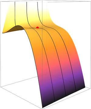
  $p_{\ell }-p_v>0$ which corresponds to desinence. The Gibbs free energy of each regime is shown in figures 2(a) and 2(b), respectively.
A free spherical bubble of radius  $r$ suspended in a partially filled container. The liquid pressure is given by $p_{\ell }$. The pressure outside the liquid and inside the bubble is the combination of vapour pressure $p_v$ and dissolved gas pressure $p_g$.

A surface plot of the Gibbs free energy  ${\rm \Delta} G_{tot}$ as a function of the radius $r$ and moles of gas $n_g$. (a) The incipient conditions when the liquid pressure is less than the vapour pressure ( $p_{\ell } < p_v$). It is worth noting that the red point denotes the saddle point which coincidentally recovers Blake's radius. (b) The desinent conditions when the liquid pressure is greater than the vapour pressure ( $p_{\ell } > p_v$). The solid black lines are the cross-sectional locations used for analysis.

Consider figure 2(a) for the incipient regime. Notice that when no gas is present,  ${\rm \Delta} G_{tot}$ goes to zero for $r=0$ and increases with increasing $r$ until it reaches a local maximum before a sharp drop in energy is observed. As the gas content increases, ${\rm \Delta} G$ forms a local minimum with decreasing $r$ and does not go to zero. The energy starts to rise again with increasing $r$ to reach a local maximum before a sharp drop. On this surface plot, the saddle point is highlighted with a red circle. Beyond the saddle point, with increasing $n_g$, the local minimum disappears and shallower gradients are observed. From this figure, we identify two key areas of interest. The first location corresponds to zero gas content which represents homogeneous nucleation, and the second location corresponds to a saturated nucleus at the saddle point. Those locations are equivalent to $f(n_g)=0$ and $f(n_g)=2$, respectively, each of which behave differently. Based on those key areas of interest, four different cross-sections are analysed based on the following intervals: the first being $f(n_g)=0$, which corresponds to a homogeneous nucleation (pure liquid–vapour); the second being in the interval of $0 < f(n_g) < 2$, where heterogeneous nucleation begins to take place but the gas is undersaturated; the third being the saddle point at $f(n_g)=2$, where the gas is saturated; and finally the fourth interval corresponding to $f(n_g)>2$, where the gas is supersaturated. For the sake of convenience, equal intervals are taken for the analysis and are summarised in table 1. One might argue that it could be sufficient to take the saddle point location as the representative case for heterogeneous nucleation in the presence of gas due to the fact the it can be interpreted as the thermodynamically preferred (and efficient) path to equilibrium. We can also show that in that particular location, it recovers Blake's radius, as discussed in our analysis in the subsequent section. However, due to the nature of nucleation, thermodynamic fluctuations do not always necessarily lead to the most efficient path. Two different time scales are at play: one is related to mechanical equilibrium (bubble growth and collapse corresponding to the change in $r$) and the other is diffusion (increasing and decreasing gas content $n_g$ in a bubble). Given any system, the response of nuclei could easily be growth in $r$ at a much faster rate to reduce ${\rm \Delta} G_{tot}$ instead of increasing $n_g$ for example to achieve stability. Hence, we explore all possible scenarios and quantify their effect on the nucleation process.
Summary of the different cases investigated and the corresponding cross-section.

Consider figure 2(b) which illustrates the second regime corresponding to desinence. For zero gas content,  ${\rm \Delta} G_{tot}$ goes to zero at $r=0$ and increases with increasing $r$. However, as the gas content in the system increases, ${\rm \Delta} G_{tot}$ does not go to zero. In fact it increases as $r$ approaches zero, decreases with increasing $r$ then increases again beyond some critical value, leading to a local minimum. This behaviour carries on with increasing gas content.
A detailed analysis of the different cross-sections of figures 2(a) and 2(b) is discussed §§ 4 and 5, respectively. The only exception is in § 5, where we do not go into a full breakdown of the cross-sectional plots for the sake of brevity, as we believe a similar analysis conducted in § 4 can be easily extended by the interested reader. The same ranges and case numbers are used for both regimes as described in table 1.
4. Incipience
For the incipient regime  $(p_{\ell }-p_v)<0$, we consider the four cases presented in table 1. We analyse each cross-section and give a physical interpretation of the nuclei behaviour in Appendix B. We investigate the critical radius required for nucleation, and generalise those expressions to include the effect of gas content. We also investigate the change in the required activation energy and the stability of the nuclei formed. The analysis highlights the effect of gas content on nucleation. We have shown that with increasing gas content, the critical radius is reduced due to the presence of gas which effectively reduces the activation energy required for phase change. Under certain circumstances, it can potentially eliminate it. The reduction in $r_{cr}$ is clearly observed over the four cases considered. One can in fact derive an analytic expression for $r_{cr}$ in the incipient regime as a function of gas content $n_g$. The details of the derivations are not shown here. The general expression is given by the following:
 \begin{align} r_{cr} &= \xi_{inc}(n_g) \frac{2 \sigma_{\ell g}}{(p_v-p_{\ell})} \nonumber\\ & = \xi_{inc}(n_g) r_{cr,v}, \end{align}
where  $\xi _{inc}(n_g)$ is the correction factor that modifies $r_{cr}$ for different gas content, such that
 \begin{equation} \xi_{inc}(n_g) =\tfrac{2}{3} \cos \{\tfrac{1}{3} \cos^{{-}1} [1-f(n_g)]\} + \tfrac{1}{3},\quad \text{for}\ 0 \le f(n_g) \le 2. \end{equation}
Figure 3 shows the variation of  $\xi _{inc}$ as a function of $n_g$. It is clear that the effective $r_{cr}$ is reduced. Note the range of validity, where beyond the threshold of $f(n_g)>2$, no activation barrier is required to nucleate as it is effectively reduced to zero. Hence, no critical radius exists beyond those values.
Value of the coefficient multiplier for the incipience case as a function of gas content.

The reduction in the critical activation energy for all the previous cases can also be summarised by the following expression:
 \begin{align} {\rm \Delta} G^*_{act} &= \xi_{act}(n_g) \left(\frac{16 {\rm \pi}\sigma^3_{\ell g}}{3 {\rm \Delta} p^2_{cr}}\right) \nonumber\\ &= \xi_{act}(n_g) {\rm \Delta} G^*_{act,v}, \end{align}
where the variation in the coefficient  $\xi _{act}(n_g)$ multiplying ${\rm \Delta} G^*_{act,v}$ can be expressed as a function of $f(n_g)$ whose analytic solution is given by
 \begin{align} \xi_{act}(n_g) &= \frac{1}{9}\left[(6\cos{\varTheta}+3\cos{2\varTheta}-2\sqrt{3} \sin{\varTheta}+\sqrt{3}\sin{2\varTheta}) \vphantom{\left(\frac{1-\cos{\varTheta}+\sqrt{3} \sin{\varTheta}}{1+2\cos{\varTheta}}\right)^3}\right.\nonumber\\ &\quad \left.+\frac{4}{3}f(n_g) \ln{\left(\frac{1-\cos{\varTheta}+\sqrt{3} \sin{\varTheta}}{1+2\cos{\varTheta}}\right)^3}\right]. \end{align}
Keep in mind that  $\varTheta =(1/3)\cos ^{-1}[1-f(n_g)]$ and was used in (4.4) for clarity. Figure 4 shows the variation of $\xi _{act}$ as a function of $f(n_g)$. It is clear that an increase in gas content reduces the required activation energy.
Value of the coefficient multiplier for the critical Gibbs energy required for activation as a function of gas content. The solid blue line is obtained from the analytic solution given by (4.4).

5. Desinence
For the desinent regime,  $(p_{\ell }-p_v)>0$. We consider the four cases presented in table 1. In § 4 we investigated the critical radius required for nucleation, but as we can observe from figure 2(b), the desinent regime can sustain nuclei since a local minimum is always present. The term ‘critical’ radius does not make much sense since there is no energy barrier to overcome. Instead, we define an equilibrium radius $r_{eq}$, and generalise those expressions to include the effect of gas content. We also investigate the stability of the nuclei formed. The analysis highlights the effect of gas content on sustaining nuclei for the desinent regime. We have shown that the equilibrium radius increases with increasing gas content. The increase in $r_{eq}$ is clearly observed over the four cases considered, as more gas can help sustain larger bubbles/nuclei. Similar to the previous section, we derive an analytic expression for $r_{eq}$ as a function of gas content that takes into account $n_g$. The general expression is given by the following:
 \begin{equation} r_{eq} = \xi_{des}(n_g)\frac{2 \sigma_{\ell g}}{(p_{\ell}-p_v)}, \end{equation}
where  $\xi _{des}(n_g)$ is the correction factor that modifies $r_{eq}$ for different gas content, such that
 \begin{equation} \xi_{des}(n_g)
=\begin{cases} \dfrac{2}{3} \cos \left\{\dfrac{1}{3}
\cos^{{-}1} [f(n_g) - 1] \right\} - \dfrac{1}{3}, &
\text{if}\ 0 \le f(n_g) \le 2 \\ \dfrac{2}{3} \cosh
\left\{\dfrac{1}{3} \cosh^{{-}1} [f(n_g) - 1] \right\} -
\dfrac{1}{3}, & \text{otherwise}.
\end{cases}\end{equation}
\begin{equation} \xi_{des}(n_g)
=\begin{cases} \dfrac{2}{3} \cos \left\{\dfrac{1}{3}
\cos^{{-}1} [f(n_g) - 1] \right\} - \dfrac{1}{3}, &
\text{if}\ 0 \le f(n_g) \le 2 \\ \dfrac{2}{3} \cosh
\left\{\dfrac{1}{3} \cosh^{{-}1} [f(n_g) - 1] \right\} -
\dfrac{1}{3}, & \text{otherwise}.
\end{cases}\end{equation}
Notice the range of validity as compared with the incipient case. There are no limitations necessarily since gas content can increase to supersaturation degrees. Figure 5 shows the variation in  $\xi _{des}$ as a function of $n_g$. With increasing gas content, we observe that larger $r_{eq}$ can be sustained. The stability argument shows that for all cases, the system is always stable and can sustain nuclei with the exception of pure liquid–vapour systems where the vapour dissolves back into the liquid.
Value of the coefficient multiplier for the desinence case as a function of gas content.

6. Hysteresis
Cavitation hysteresis is the process by which the cavitation number at which cavitation appears when the pressure is decreased is different from the cavitation number at which cavitation disappears when the pressure is raised (Holl & Treaster Reference Holl and Treaster1966; Brennen Reference Brennen2014). Notice how in figures 2(a) and 2(b) there is a clear difference in the surface plot of the Gibbs free energy between the two regimes. While certain critical radii are required to overcome the energy barrier in the incipient regime, the equilibrium radius in the desinent regime does not show a one-to-one correspondence for the same pressure difference. The critical radius required for nucleation is reduced with increasing gas content, but beyond saturation there is no energy barrier, and cavitation becomes spontaneous. This could be indicative of the two different types of ‘vaporous’ and ‘gaseous’ cavitation. In the degassing process (i.e. the desinent regime), nuclei can be maintained at  $r_{eq}$ which increases with increasing gas content, and the nuclei do not necessarily dissolve back into liquid unless it was a pure vapour. Therefore, it is expected that after cavitation inception, more nuclei can be sustained after an increase in pressure due to the increase in the population of stable nuclei. Another form of asymmetry can be observed in the constant coefficients of the incipient and desinent regimes depicted in figures 3 and 5, respectively. The coefficients of the incipient and desinent regimes correspond to (4.2) and (5.2), respectively. Note the range of validity where $\xi _{inc}(n_g)$ is limited by the saturation degree beyond which no critical radius exists. The maximum value is $1$, which recovers the homogeneous $r_{cr,v}$, and has a minimum value of $2/3$ for the saturated case, which recovers Blake's radius. In contrast, $\xi _{des}$ has a minimum value of $0$ and largely no upper bound going into supersaturation. Another difference is the rates at which these coefficients vary, thus indicating further differences that could explain the hysteresis observed experimentally. This strong dependence on the gas concentration is in agreement with Amini et al. (Reference Amini, Reclari, Sano and Farhat2019).
Table 2 shows typical values obtained from our expressions for a theoretical case. The first feature we observe is the fact that for the same value of  $|{\rm \Delta} p|$, different values for $r_{cr}$ are obtained for the case incipience versus desinence. Another feature to point out is the fact that the coefficient (a function of $n_g$) multiplying the expression $2 \sigma _{\ell g}/{\rm \Delta} p$ is different for each case, and also different in the rate it changes with varying $n_g$. Asymmetry is clearly observed. Take for example a degassing process to ensure all micro-bubbles are dissolved, the facility static pressure being controlled at $100\,\mathrm {kPa}$. For case I, no gas is present, and therefore it is expected that all micro-bubbles will dissolve back into the system. In our analysis, this corresponds to an equilibrium solution with $r_{cr}=0$ as shown in table 2, where the contracting forces dominate the expanding forces. For cases II, III and IV, it is obvious that an equilibrium solution exists, whose analysis can be found in § 3, with values for $r_{cr}=0.35$, $0.48$ and $0.57 \,\mathrm {\mu }\mathrm {m}$, respectively.
Summary of the critical radii obtained for different gas content under positive and negative pressure difference.

The takeaway point is the fact that the presence of gas will prevent the complete dissolution of all the micro-bubbles since there exists an equilibrium solution for the system. This implies that higher pressures are required to further dissolve any existing nuclei. However, on the nanoscale or angstrom scale, the ideal gas assumption fails and some modification to the model is warranted. The second implication is the asymmetry in the values of  $r_{cr}$. After the degassing process, the measurements commence as the flow rate begins to increase. At certain critical tensions, cavitation events are registered. Take for example a critical tension ${\rm \Delta} p = -100\,\mathrm {kPa}$. The critical radii obtained are $r_{cr} = 1.44$, $1.31$ and $0.96 \,\mathrm {\mu }\mathrm {m}$ for cases I, II and III, respectively. Remember that the negative value associated with case IV simply means that there is no critical radius, and that the gas–vapour bubble forms spontaneously. This is due to the fact that the expanding forces dominate the compressive forces. For the same $|{\rm \Delta} p|$, different critical radii are obtained, providing a possible explanation for the hysteresis observed between incipient and desinent events.
7. Comparison with experiments
We discuss the implications of our solutions for experimental measurements of nuclei. One method for measuring nuclei concentrations is by direct imaging, which has its set of limitations. Concentrations can be low such that they require impractically long periods of optical measurements. The size of the nuclei can also be of the order micrometres ( $0.1\,\mathrm {\mu } {\mathrm m}$), such that imaging with visible light wavelengths is beyond diffraction limits. In the presence of solid contaminants, the imaging would not reveal the volume of trapped gas but instead the size of the particle itself. These limitations are overcome by using a CSM (Oldenziel Reference Oldenziel1982; d'Agostino & Acosta Reference d'Agostino and Acosta1991; Lecoffre Reference Lecoffre1999). A CSM measures the nuclei distribution in water by passing sampled water through a venturi exposing it to a reduced pressure. The nuclei are activated at the critical pressures of the venturi, and are counted by analysing the output signal from a high-frequency piezoceramic sensor. Different cumulative histograms of nuclei concentration are obtained by varying the flow rate. The nuclei population is dependant on the dissolved gas content, the level of contaminants present in the water sample and the artificial seeding of micro-bubbles. The standard method is to use Blake's radius as a representative of the critical bubble size with dissolved gas. In our analysis, this is achieved by equating the critical pressure at initial conditions to the same equation at critical conditions. The diameter of the bubble is then obtained numerically. The method is described here for completeness and is then extended to the different cases presented earlier. At equilibrium:
 \begin{equation} p_{\ell,0} = p_v - \frac{2 \sigma_{\ell g}}{r_0} + \frac{3 n_g B T}{4 {\rm \pi}r_0^3}. \end{equation}
For a constant  $T$ and $n_g$, Blake's radius is given by
 \begin{equation} r_{cr} = \sqrt{ \frac{9 n_g B T}{8 {\rm \pi}\sigma_{\ell g}}}. \end{equation}
Substituting Blake's radius in the Laplace equation gives the following expression:
 \begin{equation} p_{\ell,0} = p_v - \frac{2 \sigma_{\ell g}}{r_0} + \frac{2 \sigma_{\ell g}}{3}\frac{r^2_{cr}}{r_0^3}. \end{equation}
Another similar expression can be obtained by substituting Blake's radius in the Laplace equation at critical conditions to get the following expression:
 \begin{equation} p_{\ell,cr} = p_v - \frac{2 \sigma_{\ell g}}{r_{cr}} + \frac{2 \sigma_{\ell g}}{3}\frac{r^2_{cr}}{r_{cr}^3}, \end{equation}
such that
 \begin{equation} r_{cr} ={-}\frac{4 \sigma_{\ell g}}{3(p_{\ell,cr}-p_v)}. \end{equation}
Therefore, we can write the equality between the initial and critical conditions as
 \begin{equation} p_{\ell,0} - p_v + \frac{2 \sigma_{\ell g}}{r_0} = \frac{2 \sigma_{\ell g}}{3}\frac{r^2_{cr}}{r_0^3}. \end{equation}
Simplifying the expression and substituting the second value of the critical radius we get the following:
 \begin{equation} \frac{4}{27(p_{\ell,cr} - p_v)^2} = (p_{\ell,0}-p_v) \left(\frac{r_0}{2 \sigma_{\ell g}}\right)^3 + \left(\frac{r_0}{2 \sigma_{\ell g}}\right)^2. \end{equation}
In terms of bubble diameter:
 \begin{equation} \frac{4}{27(p_{\ell,cr} - p_v)^2} = (p_{\ell,0}-p_v) \left(\frac{d_0}{4 \sigma_{\ell g}}\right)^3 + \left(\frac{d_0}{4 \sigma_{\ell g}}\right)^2, \end{equation}
where  $d_0$ is obtained numerically. The bubble diameter may be expressed in the cubic polynomial form
 \begin{equation} d^3_0 + \frac{4 \sigma_{\ell g}}{(p_{\ell,0}-p_v)} d^2_0 - \frac{4 \sigma_{\ell g}}{3(p_{\ell,0}-p_v)} \left[\frac{4 \sigma_{\ell g}}{3(p_{\ell,cr}-p_v)}\right]^2 = 0. \end{equation}
The details for finding the solution analytically are described in Appendix A.2. Notice that the above solution is a special case in our Gibbs free energy formulation corresponding to case III. It does not take into account the variation of  $n_g$. Therefore, a similar approach is used for the other cases whose details are not shown here. The final solution for the most general form is written as
 \begin{equation} d_0 = \xi_0(n_g) \frac{4 \sigma_{\ell g}}{(p_{\ell,0}-p_v)}, \end{equation}
where
 \begin{align} &\xi_0(n_g)\nonumber\\
&\quad =\begin{cases} \dfrac{2}{3} \cos \left\{\dfrac{1}{3}
\cos^{{-}1} \left[f(n_g)
\left(\dfrac{p_{\ell,0}-p_v}{p_{\ell,cr}-p_v}\right)^2 - 1
\right]\right\} \!-\!\dfrac{1}{3}, & \text{if}
\dfrac{|p_{\ell,cr}\!-p_v|}{|p_{\ell,0}\!-p_v|} \!\ge \!
\dfrac{\sqrt{2f(n_g)}}{2} \\ \dfrac{2}{3} \cosh
\left\{\dfrac{1}{3} \cosh^{{-}1} \left[f(n_g)
\left(\dfrac{p_{\ell,0}-p_v}{p_{\ell,cr}-p_v}\right)^2 - 1
\right]\right\} - \dfrac{1}{3}, & \text{otherwise}. \end{cases}
\end{align}
\begin{align} &\xi_0(n_g)\nonumber\\
&\quad =\begin{cases} \dfrac{2}{3} \cos \left\{\dfrac{1}{3}
\cos^{{-}1} \left[f(n_g)
\left(\dfrac{p_{\ell,0}-p_v}{p_{\ell,cr}-p_v}\right)^2 - 1
\right]\right\} \!-\!\dfrac{1}{3}, & \text{if}
\dfrac{|p_{\ell,cr}\!-p_v|}{|p_{\ell,0}\!-p_v|} \!\ge \!
\dfrac{\sqrt{2f(n_g)}}{2} \\ \dfrac{2}{3} \cosh
\left\{\dfrac{1}{3} \cosh^{{-}1} \left[f(n_g)
\left(\dfrac{p_{\ell,0}-p_v}{p_{\ell,cr}-p_v}\right)^2 - 1
\right]\right\} - \dfrac{1}{3}, & \text{otherwise}. \end{cases}
\end{align}
The practitioner who desires to obtain  $d_0$ using Blake's assumptions can simply substitute $f(n_g)=2$ into (7.11) and calculate (7.10) accordingly. We hope that this approach is useful for CSM measurements since it bypasses the need to numerically calculate $d_0$, and instead provides a more reliable and analytic solution. Figure 6 shows a comparison between the numerical solution obtained using Newton–Raphson and the analytic solution obtained in (7.10). Good agreement is observed, validating our results. The analytic results can now be used in conjunction with the experimental values obtained in Venning et al. (Reference Venning, Khoo, Pearce and Brandner2018) for cumulative background nuclei distributions $C$ as a function of critical tension. The measurements are obtained using a CSM (Pham, Michel & Lecoffre Reference Pham, Michel and Lecoffre1997; Khoo et al. Reference Khoo, Venning, Pearce, Brandner and Lecoffre2016) at the Australian Maritime College (AMC) cavitation tunnel. Furthermore, figure 7 shows a combined plot of $C$ versus ${\rm \Delta} p_{cr}$, the bubble diameter obtained analytically using (7.10) being given on the top horizontal axis, and a power-law fit is given by
 \begin{equation} C = (1.7\times10^{{-}22}) d_0^{{-}4.075}, \end{equation}
where  $C$ is given in units of $\mathrm {m}^{-3}$ and $d_0$ in $\mathrm {m}$. Note that for completeness, Venning et al. (Reference Venning, Khoo, Pearce and Brandner2018) give $C$ in units of $\mathrm {cm}^{-3}$ and $d_0$ in $\mathrm {\mu }\mathrm {m}$ which results in an expression with a modified constant given by
 \begin{equation} C = (4.84\times10^{{-}4}) d_0^{{-}4.075}. \end{equation}
Comparison between the bubble diameter obtained using the numerical solution and the bubble diameter obtained using the analytic solution.

Cumulative background nuclei distribution in the AMC cavitation tunnel. Trend line drawn in red is a power-law fit, and the symbols are experimental values. The values for  $d_0$ on the top axis are calculated using (7.10) with $f(n_g)=2$, which recovers Blake's assumption.

There are three things to note here. First, the values of  $d_0$ obtained analytically using (7.10) result in a power-law fit coefficient that matches with the values presented in Venning et al. (Reference Venning, Khoo, Pearce and Brandner2018) who obtained $d_0$ numerically. Second, the exponent of the bubble diameter follows a $-4$ power law. Third, the constant coefficient multiplying the bubble diameter term is of $\mathcal {O}(10^{-22})$ indicating a coefficient that is proportional to molecular scales. It is not of the order of the bubble diameter. Therefore, it appears that the constant coefficient and the exponent are two quasi-independent quantities involved.
In short, for a given bubble diameter, we are able to obtain a background nuclei distribution given the power-law fit. Recall that the standard methods are based on Blake's radius, which we have shown to be a special case in our derivations, specifically case III. Therefore, the gas content is fixed in some sense. In our method, we have the flexibility of varying the gas content. The effect of varying the gas content is demonstrated in figure 8 by comparing case II, case III and case IV. For the same experimental measurements, i.e.  $C$ versus ${\rm \Delta} p_{cr}$, we get different values for $d_0$, indicating that the amount of gas molecules present during the nucleation process determines different bubble size distributions. The power-law fits in SI units for case II and case IV are, respectively,
 \begin{equation} \left.\begin{gathered} C = (4.74\times10^{{-}23}) d_0^{{-}4.075} \\ C = (3.57\times10^{{-}22}) d_0^{{-}4.075}. \end{gathered}\right\} \end{equation}
The two equations can also be written as  $C=(1.35\times 10^{-4}) d_0^{-4.075}$ and $C=(1.01\times 10^{-3}) d_0^{-4.075}$, where $C$ and $d_0$ have units of $\mathrm {cm}^{-3}$ and $\mathrm {\mu } \mathrm {m}$, respectively. Notice that the variation of moles of gas influences the value of the constant coefficient multiplying the bubble diameter. Also note that in order for the power-law fit to be dimensionally consistent, the multiplier coefficient needs to have a dimension of per unit length.
Cumulative background nuclei distribution in the AMC cavitation tunnel with different trend lines corresponding to different gas content. The symbols are the experimental results. The value for  $d_0$ is calculated using (7.10) with varying gas content $f(n_g)$. The orange triangles denote case II, the blue squares denote case III, which is the baseline case that uses Blake's radius, and the green circles denote case IV. The solid lines denote the corresponding power-law fit for each case.

In Khoo et al. (Reference Khoo, Venning, Pearce, Takahashi, Mori and Brandner2020), an alternative plot is presented based on experimental CSM measurements. The bubble diameter is compared with the derivative of the cumulative nuclei distribution  $-({\partial C}/{\partial d})$. The quantitative variations in data based on measured populations from different experiments result in a power-law fit that has the following form:
 \begin{equation} \frac{\partial C}{\partial d} = A d^n,\end{equation}
where  $n$, the index of the power law, averages around $-6.2$ with high probability but also varies over $-3.4$ to $-12.9$, and the multiplier $A$ averages around $9.8\times 10^8$ with high probability but varies between $4.6\times 10^7$ and $4.3\times 10^9$. They note that the spread has no clear correlation with tunnel operating parameters nor any long-term temporal fluctuations. After an in-depth analysis of the different measuring techniques, they conclude that the data overall tend to follow a power law with an index of $-4$. We can relate the constant coefficient to the critical Gibbs free energy presented earlier in this paper to describe the nucleation process with the presence of gas. Based on Kashchiev (Reference Kashchiev2000), we can model the cumulative concentration by the following expression:
 \begin{equation} C^* = C_0 \exp \left[-\frac{{\rm \Delta} G^*_{act}}{kT}\right], \end{equation}
where  $C_0$ is the concentration of nucleation sites within the system on which clusters of the new vapour phase form and $C$ is the equilibrium concentration of critical nuclei containing $M$ molecules such that
 \begin{equation} C_0 = \frac{M}{V} = \frac{6M}{{\rm \pi} d_0^3}. \end{equation}
Therefore, we can write
 \begin{equation} C^* = \frac{6M}{\rm \pi} \exp \left[-\frac{{\rm \Delta} G^*_{act}}{kT}\right] d_0^{{-}3}, \end{equation}
and as a result
 \begin{equation} \frac{\partial C^*}{\partial d_0} ={-}\frac{18M}{\rm \pi} \exp \left[-\frac{{\rm \Delta} G^*_{act}}{kT}\right] d_0^{{-}4}, \end{equation}
which has the form of (7.15), where  $A=-(18M/{\rm \pi} ) \exp [-{\rm \Delta} G^*_{act}/kT]$ and $n=-4$. It is clear that using CNT models leads to a solution consistent with observed experimental results. Note that the $-4$ power law comes out of a volumetric term which indicates homogeneity in the nucleation process; as a result any deviation from that constant will indicate a form of heterogeneity related to solid boundaries or impurities. Also, the multiplier is also not so much dependent on macroscale conditions, but more of a function of the molecular dynamics. Thus the model provides a bridge between the molecular nanometre scales and the vapour bubble formation on the micrometre scales that eventually leads to cavitation. The model is compared with the experimental data as presented in figure 9. The CSM long-acquisition data seem to exhibit a steeper slope. This is indicative of possible heterogeneous nucleation due to solid impurities, as the likelihood of their presence increases with longer acquisition time. The solid grey lines represent our model with the following constants in increasing order: $A = (10^{10}, 10^{14}, 10^{15}, 10^{16}, 10^{17}, 10^{18}, 10^{19})$. To obtain those constants we assumed that $A$ is a function of the molecular scale. Let $M=N/k$ be a function the number of molecules $N$ and $k$ the Boltzmann constant. On the nanoscale, we expect $N$ to vary between a few and a few hundred molecules, which puts $M$ of $\mathcal {O}(10^{23}- 10^{25})$. Another argument worth testing is the validity of the concept of a detectable radius versus a critical radius that was presented in § 4. On average, $r_{det}$ was twice as large as $r_{cr}$; hence, any diameter obtained using visual instruments (e.g. holography, light scattering or laser diffraction) is scaled by half. Figure 10 illustrates the previous example. Measurements obtained visually show a better collapse in the data when scaled by $r_{det}$.
Comparison of nuclei distribution histograms  $-({\partial C}/{\partial d})$ from a variety of laboratory and environmental waters using different measurement techniques as a function of nucleus diameter $d$ at ambient pressure $p_{\inf }$. The thick grey lines come from the model presented in this paper.

Comparison of nuclei distribution histograms  $-({\partial C}/{\partial d})$ similar to figure 9 where all data obtained using visual measurement techniques (i.e. holography, light scattering or laser diffraction) have been scaled by the detectable diameter.

8. Conclusions
Cavitation inception is an important phenomenon that describes phase transition in liquid phases. Understanding the mechanism behind this phase transition provides considerable insight into how nuclei are formed and how micro-bubble populations control the inception and dynamics of cavitating flows.
The Gibbs free energy approach is used to predict cavitation inception for homogeneous nucleation, and provides a smooth continuous transition to heterogeneous nucleation which takes into account the variation of gas content, in the absence of solid impurities. This is largely ignored in the literature. It is found that the gas content stabilises nuclei formation. A stable and unstable critical radius can be present under certain gas content, and in some situations it is not present at all, implying spontaneous nucleation. This phenomenon is not observed in pure homogeneous liquid–vapour systems. The presence of gas content reduces the energy barrier required to nucleate a vapour bubble, and under certain circumstances eliminates it. This effect has been typically attributed to heterogeneous nucleation in the presence of solid impurities. The saturation levels are divided into four categories. Each case determines how much the of the energy barrier is reduced. This effect is realised experimentally when nucleation rates increase for the same critical pressure (tensile strength). Incipience and desinence can also be explained by the asymmetry observed in the critical radii obtained for favourable and unfavourable pressure gradients. We show that Blake's radius, the minimum radius possible when gas is present, is a special case of Laplace's equation, which is shown to be a saddle point on the surface plot of the Gibbs free energy. The Gibbs free energy framework results in a analytic solution for the critical radius as a function of gas content (for both the incipient and desinent regimes). An analytic expression for the activation energy barrier, as a function of gas content, is also obtained. The framework allows us to relate the initial bubble diameter to critical pressures using a cubic equation, whose analytic solution takes into account the variation of gas content. This provides an advantage of the standard method that is typically solved numerically and is a function of Blake's radius. A model for the derivative of the cumulative nuclei histogram with respect to bubble diameter is proposed. It recovers a  $-4$ power law that is observed experimentally, and has a constant multiplier that is a function of the Gibbs number (activation energy).
Funding
This work was supported by the United States Office of Naval Research (ONR) MURI (Multidisciplinary University Research Initiatives) programme under grant N00014-17-1-2676 with Dr K.-H. Kim and Dr Y.L. Young as programme managers.
Declaration of interests
The authors report no conflict of interest.
Appendix A. Cubic polynomial
In order to find the solution to the cubic polynomial, take a general cubic equation of the form
 \begin{equation} P(y) = a_3 y^3 + a_2 y^2 + a_1 y + a_0 = 0. \end{equation}
Normalise by  $a_3$ such that
 \begin{equation} P(y) = a'_3 y^3 + a'_2 y^2 + a'_1 y + a'_0 = 0, \end{equation}
where  $a'_3 = 1$. The following forms will be used to obtain the solutions to the critical radius and the initial bubble diameter problems, respectively.
A.1. Solution for the critical radius
Based on (3.8), we obtain the following values:
 \begin{equation} \left.\begin{gathered} a'_2 = \frac{2 \sigma_{\ell g}}{(p_{\ell}-p_v)}, \\ a'_1 =0 \\ \text{and}\quad a'_0 ={-} \frac{3 n_g B T}{4 {\rm \pi}(p_{\ell}-p_v)}. \end{gathered}\right\} \end{equation}
We modify the equation such that we solve for a simpler cubic polynomial:
 \begin{equation} x^3 + a''_1 x + a''_0 = 0,\end{equation}
where
 \begin{equation} \left.\begin{gathered} a''_1 ={-} \frac{{a'_2}^2}{3} ={-} \frac{4}{3}\left[\frac{\sigma_{\ell g}}{(p_{\ell}-p_v)}\right]^2 \\ \text{and}\quad a''_0 = \frac{2}{27} {a'_2}^3 + a'_0 = \frac{16}{27} \left[\frac{\sigma_{\ell g}}{(p_{\ell}-p_v)}\right]^3 - \frac{3 n_g B T}{4 {\rm \pi}(p_{\ell}-p_v)}. \end{gathered}\right\} \end{equation}
Using the following trigonometric identity:
 \begin{equation} \cos(3 \varTheta) = 4 \cos^3 \varTheta - 3 \cos \varTheta, \end{equation}
and letting  $x = m \cos \varTheta$, we can show that
 \begin{equation} x^3 + a''_1 x + a''_0 \equiv 4 \cos^3 \varTheta - 3 \cos \varTheta - \cos(3 \varTheta) \equiv m^3 \cos^3 \varTheta + a''_1 m \cos \varTheta + a''_0 \equiv 0. \end{equation}
The above expressions define the following ratios:
 \begin{equation} \frac{4}{m^3} = \frac{-3}{a''_1 m} = \frac{\cos(3 \varTheta)}{a''_0}, \end{equation}
with  $a''_1 a''_0 \ne 0$, it follows that
 \begin{equation} m = 2 \sqrt{-\frac{a''_1}{3}} = \frac{4}{3} \frac{\sigma_{\ell g}}{|(p_{\ell}-p_v)|} \end{equation}
and
 \begin{equation} \cos(3 \varTheta) = \frac{3 a''_0}{a''_1 m} = \frac{|p_{\ell}-p_v|}{(p_{\ell}-p_v)} \left\{{-}1 + \frac{81}{64{\rm \pi}} \left(\frac{n_g B T}{\sigma_{\ell g}} \right) \left[\frac{(p_{\ell}-p_v)}{\sigma_{\ell g}}\right]^2\right\}. \end{equation}
By rearranging the constants in the second term within the braces, we can write the above equation as
 \begin{equation} \cos(3 \varTheta) = \frac{3 a''_0}{a''_1 m} = \frac{|p_{\ell}-p_v|}{(p_{\ell}-p_v)} \left\{{-}1 + 2 \left(\frac{9 n_g B T}{8 {\rm \pi}\sigma_{\ell g}} \right) \left[\frac{3}{4} \frac{(p_{\ell}-p_v)}{\sigma_{\ell g}} \right]^2\right\}. \end{equation}
Note that if the value on the right-hand side (RHS) of the expression in (A11) is less than or equal to one, the value of  $\varTheta$ is straightforward. The general solution for the unknown $x$ becomes
 \begin{equation} x_k = m \cos{\varTheta_k} = \frac{4}{3} \frac{\sigma_{\ell g}}{|(p_{\ell}-p_v)|} \cos{\varTheta_k},\quad \text{for}\ k=1,2,3 , \end{equation}
where  $\varTheta _k = \varTheta + 2(k-1){\rm \pi} /3$. Otherwise, we resort to a hyperbolic solution where $\cos (3 \varTheta )$ becomes $\cosh (\textrm {i}3 \varTheta )$, and
 \begin{equation} \varTheta ={-} \frac{i}{3} \cosh^{{-}1}(\mathrm{RHS}). \end{equation}
Similarly,  $\varTheta _k$ has a similar expression. The only difference is that two solutions admit an imaginary value, and one solution remains such that the real solution is given by
 \begin{equation} x = m \cos{\varTheta} ={\pm} m \cos \left[{\rm i}\frac{\cosh^{{-}1}(\mathrm{RHS})}{3}\right] ={\pm} m \cosh \left[\frac{\cosh^{{-}1}(\mathrm{RHS})}{3}\right], \end{equation}
where the sign of the solution  $x$ is determined by the sign of the right-hand side. The desired final solution for $y$ is then given by the following expression:
 \begin{equation} y_k = x_k - \frac{a'_2}{3} = \frac{4}{3} \frac{\sigma_{\ell g}}{|(p_{\ell}-p_v)|} \cos{\varTheta_k} - \frac{2}{3}\frac{\sigma_{\ell g}}{(p_{\ell}-p_v)}.\end{equation}
A.2. Solution for the initial diameter
Based on (7.9), we obtain the following values:
 \begin{equation} \left.\begin{gathered} a'_2 = \frac{4 \sigma_{\ell g}}{(p_{\ell,0}-p_v)}, \\ a'_1 =0 \\ \text{and}\quad a'_0 ={-} \frac{4 \sigma_{\ell g}}{3 (p_{\ell,0}-p_v)} \left[\frac{4 \sigma_{\ell g}}{3 (p_{\ell,cr}-p_v)}\right]^2. \end{gathered}\right\} \end{equation}
We modify the equation such that we solve for a simpler cubic polynomial:
 \begin{equation} x^3 + a''_1 x + a''_0 = 0,\end{equation}
where
 \begin{equation} \left.\begin{gathered} a''_1 ={-} \frac{{a'_2}^2}{3} ={-} \frac{16}{3}\left[\frac{\sigma_{\ell g}}{(p_{\ell,0}-p_v)}\right]^2 \\ \text{and}\quad a''_0 = \frac{2}{27} {a'_2}^3 + a'_0 = 2 \left[\frac{4\sigma_{\ell g}}{3(p_{\ell,0}-p_v)}\right]^3 \left[1 - 2 \left(\frac{p_{\ell,0}-p_v}{p_{\ell,cr}-p_v}\right)^2 \right]. \end{gathered}\right\} \end{equation}
Let
 \begin{equation} m = 2 \sqrt{-\frac{a''_1}{3}} = \frac{8}{3} \frac{\sigma_{\ell g}}{|(p_{\ell,0}-p_v)|} \end{equation}
and
 \begin{equation} \cos(3 \varTheta) = \frac{3 a''_0}{a''_1 m} = \frac{|p_{\ell,0}-p_v|}{(p_{\ell,0}-p_v)} \left[2 \left(\frac{p_{\ell,0}-p_v}{p_{\ell,cr}-p_v} \right)^2 - 1\right]. \end{equation}
The general solution for the unknown  $x$ becomes
 \begin{equation} x_k = m \cos{\varTheta_k} = \frac{8}{3} \frac{\sigma_{\ell g}}{|(p_{\ell,0}-p_v)|} \cos{\varTheta_k},\quad \text{for}\ k=1,2,3 , \end{equation}
where  $\varTheta _k = \varTheta + 2(k-1){\rm \pi} /3$. The desired final solution for $y_k$ is then given by the following expression:
 \begin{equation} y_k = x_k - \frac{a'_2}{3} = \frac{8}{3} \frac{\sigma_{\ell g}}{|(p_{\ell,0}-p_v)|} \cos{\varTheta_k} - \frac{4}{3}\frac{\sigma_{\ell g}}{(p_{\ell,0}-p_v)}. \end{equation}
Note that for this specific case, static pressure is typically held constant such that  $(p_{\ell,0} - p_v) > 0$. The solutions $\varTheta _2$ and $\varTheta _3$ yield imaginary solutions, so we only have to take into account $\varTheta =\varTheta _1$. Therefore, the general solution simplifies to
 \begin{equation} y = \frac{4}{3} \frac{\sigma_{\ell g}}{(p_{\ell,0}-p_v)} ( 2 \cos{\varTheta} - 1 ). \end{equation}
Appendix B. Stability analysis of the Gibbs free energy
In the following analysis we focus on the incipient case with  $p_{\ell }-p_v < 0$. A similar analysis can be can be done for the desinent case but will be left out in the interest of brevity. Consider the surface plot given by figure 2 for the Gibbs free energy. Consider four different cross-sections that corresponds to cases I, II, III and IV given in table 1. Figure 11 shows the breakdown of ${\rm \Delta} G_{tot}$ and its components as a function of radius $r$. The effect of gas content is evident by the behaviour of ${\rm \Delta} G_{tot}$. With increasing gas content the critical energy required to overcome the energy barrier for nucleation is reduced. Case I corresponds to a pure liquid–vapour system (i.e. $\lim n_g \rightarrow 0$). Figure 11(a) shows a schematic of the total Gibbs free energy curve (solid black line) for the homogeneous case. The green dotted curve corresponds to $G_{bulk}$ which decreases with the third power of $r$. While the red dashed curve corresponds to $G_{int}$ which increases with the square of $r$. As a consequence, ${\rm \Delta} G_{tot}$ first increases, reaches a maximum, then decreases. Physically, this means that vapour begins to form a cluster of molecules within the liquid; hence its total free energy increases depending on the size of the cluster. If it reaches a point beyond a critical radius $r_{cr}$, growth will continue while the system's total free energy decreases. On the other hand, if the cluster size is below $r_{cr}$, then the cluster will shrink and dissolve back into the liquid. We refer to a subcritical cluster as an embryo, and one that is greater than $r_{cr}$ as a nucleus. Once a cluster becomes a nucleus and exceeds $r_{cr}$, then the nucleus will keep growing to a macroscopically detectable bubble. The growth continues until it consumes all of the metastable phase. The well-known expressions from CNT are recovered:
 \begin{equation} r_{cr} = \frac{2 \sigma_{\ell g}}{p_v-p_{\ell}} \end{equation}
and
 \begin{equation} p_{\ell,cr} = p_v - \frac{2 \sigma_{\ell g}}{r_{cr}}. \end{equation}
The maximum energy at  $r_{cr}$, given by ${\rm \Delta} G_{tot}(r_{cr})$, is the activation energy required for a nucleation event to take place. It is denoted by an activation energy ${\rm \Delta} G^*_{act}$ as shown in figure 11(a). The value for ${\rm \Delta} G^*_{act}$ is obtained by substituting the value for $r_{cr}$ in the expression of ${\rm \Delta} G_{tot}$ such that
 \begin{equation} {\rm \Delta} G^*_{act,v} = \frac{16 {\rm \pi}}{3} \frac{\sigma^3_{\ell g}}{{\rm \Delta} p_{cr}^2}, \end{equation}
where the subscript  $v$ denotes the pure liquid–vapour system. Note that in the rest of the paper, we use the same subscript to denote the relevant homogeneous quantities, e.g. $r_{cr,v}$ and ${\rm \Delta} p_{cr,v}$.
A schematic showing (a–d) four different cross-sections of the Gibbs free energy surface. The total Gibbs free energy  ${\rm \Delta} G_{tot}$ (thick solid black line), and its components, as a function of radius $r$. The red dashed line represents the free surface energy $G_{int}$, the green dotted line represents the bulk energy $G_{bulk}$ and the blue dash-dotted line represents the chemical potential $G_{chem}$. The activation energy ${\rm \Delta} G^*_{act}$ is denoted at the critical radius $r_{cr}$.

When gas is present, dissolution does not take place when  $r< r_{cr}$, and a stable gas nucleus can be achieved when $r=r_{eq}$ as shown in figure 11(b) for case II. Note how the energy barrier is reduced due to the extra contribution of the chemical potential $G_{chem}$ which varies with $\ln (1/r^3)$. The blue dash-dotted line represents $G_{chem}$ in figure 11(b–d). Further increasing the gas content leads to the reduction of the energy barrier to zero, and $r_{eq}$ and $r_{cr}$ coincide as shown in figure 11(c) for case III. Case IV shown in figure 11(d) corresponds to a spontaneous nucleation. This is where (4.1) and (4.3) capture that effect.
Figure 11 shows a detectable radius  $r_{det}$. Define the zeroth moment of energy by
 \begin{equation} \mathcal{M}_0 = \int r^0 {\rm \Delta} G_{tot}(r)\,\mathrm{d}r, \end{equation}
the total energy of the system. We argue that the system always wants to be in a baseline stable state such that  $\mathcal {M}_0=0$. When an embryo forms, it can dissolve back into the metastable phase and the condition is satisfied. Once the nucleus overcomes the energy barrier, the nuclei grow as a response (to reduce energy). Up until that point $\mathcal {M}_0>0$. Therefore, there exists a value $r$ such that the condition $\mathcal {M}_0=0$ is satisfied. That value of $r$ is what we define to be the macroscopically detectable radius $r_{det}$ such that
 \begin{align} \mathcal{M}_0 &= \int^{r_{det}}_0 \left(4{\rm \pi} \sigma_{\ell g} r^2 - \frac{4{\rm \pi}}{3}{\rm \Delta} p_{cr} r^3 \right) \mathrm{d}r \nonumber\\ &= \frac{4 {\rm \pi}}{3} \sigma_{\ell g} r^3_{det} - \frac{\rm \pi}{3}{\rm \Delta} p_{cr} r^2_{det} = 0, \end{align}
which gives the following relation:
 \begin{equation} r_{det} = \frac{4 \sigma_{\ell g}}{{\rm \Delta} p_{cr}} = 2 r_{cr}. \end{equation}
The detectable radius is exactly twice as large the critical radius required for nucleation. It is easy to see from figure 11(a) that  ${\rm \Delta} G_{tot}(r_{det}) < 0$ since $G_{bulk} > G_{int}$. Hence, the vapour bubble undergoes spontaneous growth. Therefore, it is reasonable to expect that when a cavitation bubble is detected, the measured size is that of the detectable radius and not necessarily the critical radius. Moreover, an expression for the critical tensile strength ${\rm \Delta} p_{cr}$ as a function of $r_{det}$ can then be defined as
 \begin{equation} {\rm \Delta} p_{cr} = \frac{4 \sigma_{\ell g}}{r_{det}}. \end{equation}
For the rest of the cases when gas is present, the ratio of  $r_{det}/r_{cr}$ is reduced from $2$ to a value close to $1.85$ and can be calculated numerically.
The Gibbs free energy and its first and second derivatives with respect to the bubble radius are shown in figure 12 for the four different cases. The solid blue vertical line is drawn at the critical radii indicating where  $\partial G/ \partial r$ is zero. This does not apply to case IV since no critical radius exists. Note that $\partial ^2 G/ \partial r^2$ is negative for cases I and II, indicating a maximum for ${\rm \Delta} G_{tot}$ at $r_{cr}$ as expected. It is positive for $r_{eq}$ in case II, indicating a stable minimum, and is zero for cases III and IV, indicating neutral stability. For case I, when $r=0$, ${\rm \Delta} G_{tot} = 0$ indicating a metastable state where $\partial ^2 G/ \partial r^2$ is positive. The equilibrium at $r_{cr}$ where $\partial G/ \partial r = 0$ conveniently recovers the well-known Laplace equation (B2). Metastability of a gaseous embryo is achieved in case II at $r=r_{eq}$ and when ${\rm \Delta} G_{tot} \neq 0$. Case III recovers Blake's solution when $\partial G/\partial r = \partial G^2/ \partial r^2=0$. The stability of the system can be derived by a Taylor expansion to model small perturbations about $r_{cr}$. The perturbations are represented by the red arrows in figure 12 extending in both the expanding and shrinking directions. The following analysis of the stability of the system can thus be performed. Define a quantity $\mathcal {F}(r)$ as the force that encourages a radius change (e.g. radial perturbation). From the definition of a potential, we can then write $\mathcal {F}(r)$ as
 \begin{equation} \mathcal{F}(r) = \left.-\frac{\partial G}{\partial r}\right|_{r_{cr}}.\end{equation}
Therefore, the criteria for stability at  $r_{cr}$ are defined as follows:
 \begin{equation} \left.\begin{gathered} \text{for stability:} \quad \frac{\mathrm{d} \mathcal{F}}{\mathrm{d} r} < 0 \\ \text{for instability:} \quad \frac{\mathrm{d} \mathcal{F}}{\mathrm{d} r} \ge 0 . \end{gathered}\right\} \end{equation}
Mathematically, (B8) can be viewed as a Taylor series expansion of the force in a region near  $r_{cr}$, such that

The signs of the different components in (
B10) can be extracted from figure 12. The perturbations in the radius will cause the nucleus to either collapse or grow spontaneously depending on the signs of the components. The analysis can be expanded for all the different cases in a straightforward manner.
A schematic of the Gibbs free energy  $G$ (top), its first derivative $\partial G/\partial r$ (middle) and second derivative $\partial ^2 G/ \partial r^2$ (bottom) with respect to the radius $r$ for (a–d) the four different cross-sections considered. The blue lines highlight the location of the equilibrium or critical radius ( $r_{eq}$ and $r_{cr}$, respectively). The red arrow denotes a small perturbation about $r_{cr}$.


 Open access