

1 Introduction
In 1936, Alan Turing published a seminal paper [Reference TuringTur36] which is rightly considered foundational for modern computer science. The main subject of his paper, as seen from the title, was the concept of a computable real number. Informally, such numbers can be approximated to an arbitrary desired precision using some algorithm. Turing formalized the latter as a Turing machine (TM), which is now the commonly accepted theoretical model of computation. Appearing before actual computers, TMs can be somewhat cumbersome to describe, but their computational power is equivalent to those of programs in a modern programming language, such as Python, for instance. Let
 $$ \begin{align*}{\mathbb{D}}=\{p2^q, \;p,q\in{\mathbb{Z}}\}\end{align*} $$
denote the set of dyadic rationals. A number
 $x\in {\mathbb {R}}$
is computable if there exists a TM M, which has a single input
$x\in {\mathbb {R}}$
is computable if there exists a TM M, which has a single input
 $n\in {\mathbb {N}}$
and which outputs
$n\in {\mathbb {N}}$
and which outputs
 $d_n\in {\mathbb {D}}$
such that
$d_n\in {\mathbb {D}}$
such that
 $$ \begin{align*}|x-d_n|<2^{-n}.\end{align*} $$
The dyadic notation here is purely to support the intuition that modern computers operate in binary; replacing
 $2^{-n}$
with any other constructive bound, such as, for instance,
$2^{-n}$
with any other constructive bound, such as, for instance,
 $n^{-1}$
, would result in an equivalent definition.
$n^{-1}$
, would result in an equivalent definition.
Since there are only countably many programs in Python, there are only countably many computable numbers. Yet, it is surprisingly nontrivial to present an example of one. To this end, Turing introduced an algorithmically unsolvable problem, now known as the Halting Problem: determine algorithmically whether a given TM halts or runs forever. Turing showed that there does not exist a program M whose input is another program
 $M_1$
and whose output is
$M_1$
and whose output is
 $1$
if
$1$
if
 $M_1$
halts, and
$M_1$
halts, and
 $0$
if
$0$
if
 $M_1$
does not halt.
$M_1$
does not halt.
From this, a non-computable real is constructed as follows. Let us enumerate all programs
 $$ \begin{align*}M_1,M_2,\ldots,M_n,\ldots\end{align*} $$
in some explicit way. For instance, all possible finite combinations of symbols in the Python alphabet can be listed in the lexicographic order. Some of these programs will not run at all (and thus halt by definition) but some will run without ever halting. Let the halting predicate
 $p(n)$
be equal to
$p(n)$
be equal to
 $1$
if
$1$
if
 $M_n$
halts and
$M_n$
halts and
 $0$
otherwise.
$0$
otherwise.
Now, set
 $$ \begin{align*}\alpha=\sum_{n\geq 1}p(n)3^{-n}.\end{align*} $$
This number is clearly non-computable – an algorithm computing it could be used to determine the value of the halting predicate for every given n, and thus cannot exist.
It is worth noting a further property of
 $\alpha $
. Let us say that
$\alpha $
. Let us say that
 $x\in {\mathbb {R}}$
is left-computable if there exists a TM M which outputs an increasing sequence
$x\in {\mathbb {R}}$
is left-computable if there exists a TM M which outputs an increasing sequence
 $$ \begin{align*}a_n\nearrow x.\end{align*} $$
There are, again, only countably many left-computable numbers, and it is trivial to see that computable numbers form their subset (a proper subset, as seen below). Right computability is defined in the same way with decreasing sequences, and it is a nice exercise to show that being simultaneously left- and right-computable is equivalent to being computable.
The non-computable number
 $\alpha $
is left-computable, as it is the limit of
$\alpha $
is left-computable, as it is the limit of
 $$ \begin{align*}\alpha_n=\underset{j\leq n \;|\; M_j\text{ halts in at most }n\text{ steps }}{\sum}3^{-j},\end{align*} $$
which can be generated by a program which emulates
 $M_1,\ldots ,M_k$
for k steps to produce
$M_1,\ldots ,M_k$
for k steps to produce
 $\alpha _k$
.
$\alpha _k$
.
Since Turing, examples of non-computable reals were typically constructed along similar lines. In the 2000s, working on problems of computability in dynamics, M. Braverman and the second author discovered that non-computability may be produced via an analytic expression [Reference Braverman and YampolskyBY09]. This expression came in the form of the Brjuno function
 ${{\mathcal B}}(\theta )$
which was introduced by Yoccoz [Reference YoccozYoc96] to study linearization problems of irrationally indifferent dynamics. We will discuss
${{\mathcal B}}(\theta )$
which was introduced by Yoccoz [Reference YoccozYoc96] to study linearization problems of irrationally indifferent dynamics. We will discuss
 ${{\mathcal B}}(\theta )$
and its various cousins in detail below, but let us give an explicit formula here. For
${{\mathcal B}}(\theta )$
and its various cousins in detail below, but let us give an explicit formula here. For
 $\theta \in (0,1)\setminus {\mathbb {Q}}$
, we have
$\theta \in (0,1)\setminus {\mathbb {Q}}$
, we have
 $$ \begin{align*}{{\mathcal B}}(\theta)=\sum_{n\geq 0}\theta_{-1}\theta_0\theta_1\dots\theta_{n-1}\log\frac{1}{\theta_n}.\end{align*} $$
Here,
 $\theta _{-1}=1$
,
$\theta _{-1}=1$
,
 $\theta _0\equiv \theta $
, and
$\theta _0\equiv \theta $
, and
 $\theta _{i+1}$
is obtained from
$\theta _{i+1}$
is obtained from
 $\theta _i$
by applying the Gauss map
$\theta _i$
by applying the Gauss map
 $x\mapsto \{1/x\}$
. Of course, for rational values of
$x\mapsto \{1/x\}$
. Of course, for rational values of
 $\theta ,$
the summand will eventually turn infinite. The sum may also diverge for an irrational
$\theta ,$
the summand will eventually turn infinite. The sum may also diverge for an irrational
 $\theta $
, and yet can be shown to converge to a finite value for almost all values in
$\theta $
, and yet can be shown to converge to a finite value for almost all values in
 $(0,1)$
.
$(0,1)$
.
It is evident that if
 $\theta $
is computable, then
$\theta $
is computable, then
 ${{\mathcal B}}(\theta )$
is left-computable. Very surprisingly, this can be reversed in the following way. Setting
${{\mathcal B}}(\theta )$
is left-computable. Very surprisingly, this can be reversed in the following way. Setting
 $$ \begin{align*}y_*\equiv\inf\{{{\mathcal B}}(\theta),\;\theta\in(0,1)\},\end{align*} $$
for each left-computable
 $y\in [y_*,\infty ),$
there exists a computable
$y\in [y_*,\infty ),$
there exists a computable
 $\theta \in (0,1)$
with
$\theta \in (0,1)$
with
 ${{\mathcal B}}(\theta )=y$
. The Brjuno function can be seen as a “machine” mapping computable values in
${{\mathcal B}}(\theta )=y$
. The Brjuno function can be seen as a “machine” mapping computable values in
 $(0,1)$
surjectively onto left-computable values in
$(0,1)$
surjectively onto left-computable values in
 $[y_*,\infty )$
.
$[y_*,\infty )$
.
Moreover, there exists an explicit algorithm
 $\hat M$
which, given a sequence
$\hat M$
which, given a sequence
 $a_n\nearrow y$
, computes
$a_n\nearrow y$
, computes
 $\theta $
such that
$\theta $
such that
 ${{\mathcal B}}(\theta )=y$
. Taking Turing’s non-computable
${{\mathcal B}}(\theta )=y$
. Taking Turing’s non-computable
 $\alpha $
, as we saw above, there is an explicit program to produce a sequence of rationals
$\alpha $
, as we saw above, there is an explicit program to produce a sequence of rationals
 $\alpha _n\nearrow \alpha $
. “Feeding” the sequence
$\alpha _n\nearrow \alpha $
. “Feeding” the sequence
 $\alpha _n$
to
$\alpha _n$
to
 $\hat M,$
we obtain an explicitly computable
$\hat M,$
we obtain an explicitly computable
 $\theta _*$
for which
$\theta _*$
for which
 ${{\mathcal B}}(\theta _*)=\alpha $
. This example demonstrates that
${{\mathcal B}}(\theta _*)=\alpha $
. This example demonstrates that
 ${{\mathcal B}}(\theta )$
is a natural analytic mechanism for producing non-computable reals.
${{\mathcal B}}(\theta )$
is a natural analytic mechanism for producing non-computable reals.
The purpose of this article is as follows. We distill the proof of the above result from [Reference Braverman and YampolskyBY09], where it is somewhat hidden in the considerations of complex dynamics and Julia sets. Moreover, we generalize the result to cover other Brjuno-type functions which have previously appeared in the mathematical literature, some of them 60 years before Yoccoz’s work and in a completely different context. Our generalization describes the phenomenon in the language of dynamical systems. As we will see, ergodic sampling of a particular type of dynamics with suitable weights leads to non-computability.
Finally, for an even broader natural class of functions, which have also previously been studied, and which do not quite fit the above framework, we prove a more general, albeit weaker, non-computability result.
2 Preliminaries
2.1 Computable functions
The “modern” definition of a computable function requires the concept of an oracle. Loosely speaking, an oracle for a real number x, for example, is a user who knows x and, when queried by a TM, can input its value with any desired precision. In the world of TMs (as well as Python programs), an oracle may be conceived as an infinite tape on which an infinite string of dyadic rationals is written (encoding, for instance, a Cauchy sequence for
 $x\in {\mathbb {R}}$
) and which the program is able to read at will. Of course, only a finite amount of information can be read off this tape each time. As well as a real number, an oracle can be used to encode anything else which could be written on an infinite tape, for instance, the magically obtained solution to the Halting Problem.
$x\in {\mathbb {R}}$
) and which the program is able to read at will. Of course, only a finite amount of information can be read off this tape each time. As well as a real number, an oracle can be used to encode anything else which could be written on an infinite tape, for instance, the magically obtained solution to the Halting Problem.
Formally, an oracle is a function
 $\phi :{\mathbb {N}}\to {\mathbb {D}}$
. An oracle for
$\phi :{\mathbb {N}}\to {\mathbb {D}}$
. An oracle for
 $x\in {\mathbb {R}}$
satisfies
$x\in {\mathbb {R}}$
satisfies
 $$ \begin{align*} |\phi(n) - x| < 2^{-n} \text{ for all } n \in \mathbb{N}. \end{align*} $$
We say a TM
 $M^{\phi }$
is an oracle Turing Machine if at any step of the computation,
$M^{\phi }$
is an oracle Turing Machine if at any step of the computation,
 $M^{\phi }$
can query the value
$M^{\phi }$
can query the value
 $\phi (n)$
for any n. We treat an oracle TM as a function of the oracle; that is, we think of
$\phi (n)$
for any n. We treat an oracle TM as a function of the oracle; that is, we think of
 $\phi $
in
$\phi $
in
 $M^{\phi }$
as a placeholder for any oracle, and the TM performs its computational steps depending on the particular oracle it is given. We will talk about “querying the oracle,” “being given the access to an oracle for x,” or just “given
$M^{\phi }$
as a placeholder for any oracle, and the TM performs its computational steps depending on the particular oracle it is given. We will talk about “querying the oracle,” “being given the access to an oracle for x,” or just “given
 $x.$
”
$x.$
”
We need oracle TMs to define computable functions on the reals. For
 $S\subset {\mathbb {R}}$
, we say that a function
$S\subset {\mathbb {R}}$
, we say that a function
 $f:S\to {\mathbb {R}}$
is computable if there exists an oracle TM
$f:S\to {\mathbb {R}}$
is computable if there exists an oracle TM
 $M^\phi $
with a single input n such that for any
$M^\phi $
with a single input n such that for any
 $x\in S,$
the following is true. If
$x\in S,$
the following is true. If
 $\phi $
is an oracle for x, then upon input n, the machine
$\phi $
is an oracle for x, then upon input n, the machine
 $M^\phi $
outputs
$M^\phi $
outputs
 $d_n\in {\mathbb {D}}$
such that
$d_n\in {\mathbb {D}}$
such that
 $$ \begin{align*}|f(x)-d_n|<2^{-n}.\end{align*} $$
In other words, there is an algorithm which can output the value of
 $f(x)$
with any desired precision if it is allowed to query the value of x with an arbitrary finite precision.
$f(x)$
with any desired precision if it is allowed to query the value of x with an arbitrary finite precision.
The domain of the real-valued function plays an important role in the above definition. The definition states that there is a single algorithm which, given x, works for every
 $x \in S$
. We will abbreviate this by saying that f is uniformly computable on S.
$x \in S$
. We will abbreviate this by saying that f is uniformly computable on S.
In the case when S is a singleton,
 $S=\{x_0\},$
we will say that the function
$S=\{x_0\},$
we will say that the function
 $f(x)$
is computable at the point
$f(x)$
is computable at the point
 $x_0$
. Evidently, the weakest computability result and the strongest non-computability result one can obtain in regards to real-valued functions is when the domain is restricted to a single point.
$x_0$
. Evidently, the weakest computability result and the strongest non-computability result one can obtain in regards to real-valued functions is when the domain is restricted to a single point.
It is worth making note of the following easy fact, whose proof we leave as an exercise.
Proposition 2.1 If f is uniformly computable on
 $S,$
then f is continuous on S.
$S,$
then f is continuous on S.
Uniform left- or right-computability of functions is defined in a completely analogous way.
2.2 Brjuno function and friends
Every irrational number
 $\theta $
in the unit interval admits a unique (simple) continued fraction expansion:
$\theta $
in the unit interval admits a unique (simple) continued fraction expansion:
 $$ \begin{align*} [a_{1}, a_{2}, a_{3}, \ldots] \equiv \cfrac{1}{a_{1}+\cfrac{1}{a_{2}+\cfrac{1}{a_{3}+\dots}}} \in (0,1)\setminus\mathbb{Q}, \end{align*} $$
where
 $a_{i} \in {\mathbb {N}}$
. An important related concept is that of the Gauss map
$a_{i} \in {\mathbb {N}}$
. An important related concept is that of the Gauss map
 $G:(0,1]\to [0,1]$
given by
$G:(0,1]\to [0,1]$
given by
 $$ \begin{align*} G(x) = \left\{\frac{1}{x}\right\}; \end{align*} $$
it has the property
 $$ \begin{align*}G([a_{1}, a_{2}, a_{3}, \ldots]) = [a_{2}, a_{3}, a_{4}, \ldots].\end{align*} $$
In what follows, for a function F, we denote
 $F^{n}$
its n-th iterate. For ease of notation, for each
$F^{n}$
its n-th iterate. For ease of notation, for each
 $j\in {\mathbb {N,}}$
let us define the function
$j\in {\mathbb {N,}}$
let us define the function
 $\eta _{j}: (0, 1) \setminus \mathbb {Q} \to (0, 1) \setminus \mathbb {Q}$
as
$\eta _{j}: (0, 1) \setminus \mathbb {Q} \to (0, 1) \setminus \mathbb {Q}$
as
 $ \eta _{j}(x) = G^{j-1}(x)$
, so that
$ \eta _{j}(x) = G^{j-1}(x)$
, so that
 $$ \begin{align*}\eta_{j}([a_{1}, a_{2}, a_{3}, \ldots]) = [a_{j}, a_{j+1}, a_{j+2}, \ldots].\end{align*} $$
We define Yoccoz’s Brjuno function, or for brevity, just the Brjuno function [Reference YoccozYoc96] by
 $$ \begin{align} {{\mathcal B}}(x) = \sum_{i=1}^{\infty} \eta_{0}(x) \eta_{1}(x) \dots \eta_{i-1}(x) \cdot (-\log(\eta_{i}(x))), \end{align} $$
where we set
 $\eta _{0}(x) = 1$
for all x. Irrationals in
$\eta _{0}(x) = 1$
for all x. Irrationals in
 $(0,1)$
for which
$(0,1)$
for which
 ${{\mathcal B}}(x)<+\infty $
are known as Brjuno numbers; they form a full measure subest of
${{\mathcal B}}(x)<+\infty $
are known as Brjuno numbers; they form a full measure subest of
 $(0,1)$
. The original work of Brjuno [Reference BrjunoBrj71] characterized Brjuno numbers using a different infinite series, whose convergence is equivalent to that of (2.1).
$(0,1)$
. The original work of Brjuno [Reference BrjunoBrj71] characterized Brjuno numbers using a different infinite series, whose convergence is equivalent to that of (2.1).
The Brjuno condition has been introduced in the study of the linearization of neutral fixed points. The function
 ${{\mathcal B}}$
has an important geometric meaning in this context as an estimate on the size of the domain of definition of a linearizing coordinate. It has a number of remarkable properties and has been studied extensively (see, for instance, [Reference Marmi, Moussa and YoccozMMY97]).
${{\mathcal B}}$
has an important geometric meaning in this context as an estimate on the size of the domain of definition of a linearizing coordinate. It has a number of remarkable properties and has been studied extensively (see, for instance, [Reference Marmi, Moussa and YoccozMMY97]).
Intuitively, the condition
 ${{\mathcal B}}(x)<+\infty $
is a Diophantine-type condition; if x is a Diophantine number, then it can be shown that the series (2.1) is majorized by a geometric series. As we have learned from a talk by Marmi [Reference MarmiMar22], similar expressions have appeared much earlier in the theory of Diophantine approximation. Notably, in 1933, Wilton [Reference WiltonWil33] defined the sums
${{\mathcal B}}(x)<+\infty $
is a Diophantine-type condition; if x is a Diophantine number, then it can be shown that the series (2.1) is majorized by a geometric series. As we have learned from a talk by Marmi [Reference MarmiMar22], similar expressions have appeared much earlier in the theory of Diophantine approximation. Notably, in 1933, Wilton [Reference WiltonWil33] defined the sums
 $$ \begin{align} {{\mathcal W}}_{1}(x) &= \sum_{i=1}^{\infty} \eta_{0}(x) \eta_{1}(x) \dots \eta_{i-1}(x) \cdot (-\log^{2}(\eta_{i}(x))), \end{align} $$
 $$ \begin{align} {{\mathcal W}}_{2}(x) &= \sum_{i=1}^{\infty} (-1)^{i+1} \cdot \eta_{0}(x) \eta_{1}(x) \dots \eta_{i-1}(x) \cdot (-\log(\eta_{i}(x))), \end{align} $$
which we will call the first and second Wilton functions, respectively.
To illustrate how different the application of Wilton’s functions is from the Brjuno function, let us quote Wilton’s results. If we denote
 $d(n)$
to be the number of divisors of a positive integer n, Wilton showed that
$d(n)$
to be the number of divisors of a positive integer n, Wilton showed that
 $$ \begin{align*} \sum_{n=1}^{\infty} \dfrac{d(n)}{n} \cos 2\pi nx < \infty &\text{ if and only if } {{\mathcal W}}_{1}(x) < \infty, \text{ and} \\ \sum_{n=1}^{\infty} \dfrac{d(n)}{n} \sin 2\pi nx < \infty &\text{ if and only if } {{\mathcal W}}_{2}(x) < \infty. \end{align*} $$
One important generalization of the simple continued fraction expansion of an irrational number is the
 $\alpha $
-continued fraction expansion for
$\alpha $
-continued fraction expansion for
 $\alpha \in [1/2, 1]$
. Let
$\alpha \in [1/2, 1]$
. Let
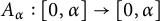 $A_{\alpha } : [0, \alpha ] \to [0, \alpha ]$
be the map
$A_{\alpha } : [0, \alpha ] \to [0, \alpha ]$
be the map
 $$ \begin{align*} A_{\alpha}(0) = 0, A_{\alpha}(s) = \left| \dfrac{1}{x} - \left\lfloor \dfrac{1}{x} - \alpha + 1 \right\rfloor \right|, x \neq 0. \end{align*} $$
By iterating this mapping, we define the infinite
 $\alpha $
-continued fraction expansion for any
$\alpha $
-continued fraction expansion for any
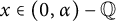 $x \in (0, \alpha ) - \mathbb {Q}$
as follows. For
$x \in (0, \alpha ) - \mathbb {Q}$
as follows. For
 $n \geq 0,$
we let
$n \geq 0,$
we let
 $$ \begin{align*} & x_{0} = |x - \lfloor x - \alpha + 1 \rfloor|, a_{0} = \lfloor x - \alpha + 1 \rfloor, \varepsilon_{0} = 1,\\ & x_{n+1} = A_{\alpha}(x_{n}) = A_{\alpha}^{n+1}(x), a_{n+1} = \left\lfloor \dfrac{1}{x_{n}} - \alpha + 1 \right\rfloor \geq 1, \varepsilon_{n+1} = \text{sgn}(x_{n}). \end{align*} $$
Then, we can write
 $$ \begin{align*} x = [(a_{1}, \varepsilon_{1}), (a_{2}, \varepsilon_{2}), \ldots, (a_{n}, \varepsilon_{n}), \ldots] := \dfrac{\varepsilon_{0}}{a_{1}+\dfrac{\varepsilon_{1}}{a_{2}+\dfrac{\varepsilon_{2}}{a_{3}+\dots}}} \in (0,\alpha)-\mathbb{Q}. \end{align*} $$
Note that when
 $\alpha =1$
, we recover the standard continued fraction expansion.
$\alpha =1$
, we recover the standard continued fraction expansion.
Generalizations of the Brjuno function based on the above expansions have been studied, for example, in [Reference Luzzi, Marmi, Nakada and NatsuiLMNN10]. There, the authors considered the properties of the function
 $$ \begin{align} {{\mathcal B}}_{\alpha, u}(x) = \sum_{i=1}^{\infty} \eta_{\alpha,0}(x) \eta_{\alpha,1}(x) \dots \eta_{\alpha,i-1}(x) \cdot u(\eta_{\alpha,i}(x)), \end{align} $$
where
 $\eta _{\alpha ,0}(x) = 1$
,
$\eta _{\alpha ,0}(x) = 1$
,
 $\eta _{\alpha , j}(x) = A_{\alpha }^{j-1}(x), \alpha \in [1/2, 1], j \geq 1$
is a generalization of
$\eta _{\alpha , j}(x) = A_{\alpha }^{j-1}(x), \alpha \in [1/2, 1], j \geq 1$
is a generalization of
 $\eta _{j}$
to alpha-continued fraction maps, and
$\eta _{j}$
to alpha-continued fraction maps, and
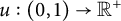 $u:(0, 1) \to \mathbb {R}^{+}$
is a
$u:(0, 1) \to \mathbb {R}^{+}$
is a
 $\mathcal {C}^{1}$
function such that
$\mathcal {C}^{1}$
function such that
 $$ \begin{align*} \lim_{x\to0^{+}}u(x) = \infty, \lim_{x\to0^{+}}x \cdot u(x) < \infty, \lim_{x\to0^{+}}x^{2} \cdot u'(x) < \infty. \end{align*} $$
A further generalized class
 $\{{{\mathcal B}}_{\alpha , u, \nu }\}$
of Brjuno functions is discussed in [Reference Bakhtawar, Carminati and MarmiBCM24], where the last two conditions above are dropped and the term
$\{{{\mathcal B}}_{\alpha , u, \nu }\}$
of Brjuno functions is discussed in [Reference Bakhtawar, Carminati and MarmiBCM24], where the last two conditions above are dropped and the term
 $\eta _{\alpha ,1}(x) \eta _{\alpha ,2}(x) \dots \eta _{\alpha ,i-1}(x)$
is raised to some power
$\eta _{\alpha ,1}(x) \eta _{\alpha ,2}(x) \dots \eta _{\alpha ,i-1}(x)$
is raised to some power
 $\nu \in \mathbb {Z}^{+}$
:
$\nu \in \mathbb {Z}^{+}$
:
 $$ \begin{align} {{\mathcal B}}_{\alpha, u, \nu}(x) = \sum_{i=1}^{\infty} (\eta_{\alpha,0}(x) \eta_{\alpha,1}(x) \dots \eta_{\alpha,i-1}(x))^{\nu} \cdot u(\eta_{\alpha,i}(x)). \end{align} $$
As shown in [Reference Bakhtawar, Carminati and MarmiBCM24]:
Proposition 2.2 For all
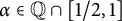 $\alpha \in \mathbb {Q} \cap [1/2, 1]$
, such functions
$\alpha \in \mathbb {Q} \cap [1/2, 1]$
, such functions
 ${{\mathcal B}}_{\alpha , u, \nu }$
are lower semi-continuous and thus attain their global minima.
${{\mathcal B}}_{\alpha , u, \nu }$
are lower semi-continuous and thus attain their global minima.
Note that if we take
 $\alpha =1$
,
$\alpha =1$
,
 $\nu =1$
, and
$\nu =1$
, and
 $u = -\log $
, we recover Yoccoz’s Brjuno function discussed above; similarly, taking
$u = -\log $
, we recover Yoccoz’s Brjuno function discussed above; similarly, taking
 $\alpha =1$
,
$\alpha =1$
,
 $\nu =1$
, and
$\nu =1$
, and
 $u = -\log ^{2}$
recovers the first Wilton function
$u = -\log ^{2}$
recovers the first Wilton function
 ${{\mathcal W}}_{1}$
. Note, however, that we cannot obtain
${{\mathcal W}}_{1}$
. Note, however, that we cannot obtain
 ${{\mathcal W}}_{2}$
as a special case of
${{\mathcal W}}_{2}$
as a special case of
 ${{\mathcal B}}_{\alpha , u, \nu }$
.
${{\mathcal B}}_{\alpha , u, \nu }$
.
3 Statements of the results
3.1 A general framework
We refer the readers to the survey [Reference Marmi, Moussa and YoccozMMY06] which discusses a cohomological interpretation of the Brjuno function and lays the groundwork for its generalizations. Our discussion will be much less technical, yet essentially equivalent in the cases we consider. It will yield a generalization which is (a) broad enough to include the relevant examples we have quoted and (b) captures the essence of the non-computability phenomenon discovered in [Reference Braverman and YampolskyBY09]. This is achieved via the following framework. Suppose
 $G(x)$
is a piecewise-defined expanding mapping whose domain is an infinite collection of subintervals of
$G(x)$
is a piecewise-defined expanding mapping whose domain is an infinite collection of subintervals of
 $(0,1),$
each of which is mapped surjectively over all of
$(0,1),$
each of which is mapped surjectively over all of
 $(0,1)$
. Let
$(0,1)$
. Let
 $\psi :(0,1)\to {\mathbb {R}}$
(in our case,
$\psi :(0,1)\to {\mathbb {R}}$
(in our case,
 $\psi (x)=x^\nu $
), and consider the skew product dynamics given by
$\psi (x)=x^\nu $
), and consider the skew product dynamics given by
 $$ \begin{align} F:\left(\begin{array}{c}x\\y\end{array}\right)=\left(\begin{array}{c}G(x)\\\psi(x) y\end{array}\right). \end{align} $$
The class of functions
 ${{\mathcal F}}$
for which non-computability arises is produced by additive (ergodic) sampling of orbits
${{\mathcal F}}$
for which non-computability arises is produced by additive (ergodic) sampling of orbits
 $(x_n,y_n)$
of F using a suitable weight function
$(x_n,y_n)$
of F using a suitable weight function
 $u(x,y)\equiv u(x)$
with positive values:
$u(x,y)\equiv u(x)$
with positive values:
 $$ \begin{align} {{\mathcal F}}(x)=\sum_{i=1}^{\infty} y_n \cdot u(x_n). \end{align} $$
It is worth noting that such a function is a formal solution of the twisted cohomological equation
 $$ \begin{align*}{{\mathcal F}}-\psi \cdot {{\mathcal F}}\circ G=u.\end{align*} $$
As noted above, in our case, we set
 $$ \begin{align*}\psi(x)\equiv x^\nu.\end{align*} $$
We will now need to make somewhat technical but straightforward general assumptions on G and u.
Let
 $G: (0, 1) \to (0, 1)$
be a function which is
$G: (0, 1) \to (0, 1)$
be a function which is
 $\mathcal {C}^{1}$
on a set
$\mathcal {C}^{1}$
on a set
 $S \subseteq (0, 1)$
, with
$S \subseteq (0, 1)$
, with
 $s_{0} := \inf S$
,
$s_{0} := \inf S$
,
 $s_{1} := \sup S$
. Suppose that for a countable collection of disjoint open intervals
$s_{1} := \sup S$
. Suppose that for a countable collection of disjoint open intervals
 $J_{i} = (\ell _{i}, r_{i})$
with
$J_{i} = (\ell _{i}, r_{i})$
with
 $\ell _{1}> \ell _{2} > \cdots $
, we have
$\ell _{1}> \ell _{2} > \cdots $
, we have
 $S = J_{1} \sqcup J_{2} \sqcup J_{3} \sqcup \cdots $
. Below, we will denote
$S = J_{1} \sqcup J_{2} \sqcup J_{3} \sqcup \cdots $
. Below, we will denote
 $G_{i} := G|_{J_{i}}$
, so that
$G_{i} := G|_{J_{i}}$
, so that
 $G_{i}^{-1}: (s_{0}, s_{1}) \to J_{i}$
is the unique branch of
$G_{i}^{-1}: (s_{0}, s_{1}) \to J_{i}$
is the unique branch of
 $G^{-1}$
mapping into
$G^{-1}$
mapping into
 $J_{i}$
. We assume that G satisfies the following criteria:
$J_{i}$
. We assume that G satisfies the following criteria:
-
(i)
 $G(J_{i}) = (s_{0}, s_{1})$
for each i.
$G(J_{i}) = (s_{0}, s_{1})$
for each i. -
(ii)
$|G'|>1$
, and additionally there exist
$\tau>1, \sigma >1$
, and
$\kappa \in \mathbb {Z}$
such that if we let then we have both
$$ \begin{align*} \tau_{i, 1} := \inf_{x \in J_{i}} \left| G'(x) \right|, \tau_{i, \kappa} := \inf_{x \in J_{i}} \left| (G^{\kappa})'(x) \right|, \end{align*} $$
$\tau _{i, 1}^{-1} < \ell _{i} \cdot \sigma $
and
$\tau _{i, \kappa }^{-1} < \ell _{i} \cdot \tau ^{-1}$
for all i. In particular, since
$\ell _{i} \leq s_{1} < 1$
, this means that
$|(G^{\kappa })'(x)|> \tau $
for all
$x \in (s_{0}, s_{1})$
.
-
(iii)
$G_{1}$
is decreasing on
$J_{1}$
. -
(iv) Let
$\varphi $
be the unique fixed point of
$G_{1}$
, and let
$\delta _{G}(N) := G_{N}^{-1}(\varphi )- G_{N+1}^{-1}(\varphi )>0$
. Then, there is some constant
$D>0$
such that for all
$N \in \mathbb {Z}^{+}$
,
$$ \begin{align*} \dfrac{r_{N+1}}{\ell_{N+1}} \cdot \dfrac{r_{N}-\ell_{N+1}}{\delta_{G}(N)} < D. \end{align*} $$
-
(v) We have
$\dfrac {r_{i}-\ell _{i}}{\ell _{i}^{2}} < D$
for some constant
$D>0$
independent of i. -
(vi) G is computable on its domain.
-
(vii)
$g(i) := \dfrac {r_{i}}{\ell _{i+1}} - 1 \to 0$
as
$i \to \infty $
. Note that since g is positive and bounded from above, there is some constant
$m_{g}>0$
for which
$0 < g(i) \leq m_{g}$
.


It is easy to show that properties (i) and (ii) imply that G restricted to the set
 $\Lambda = \bigcap _{j=0}^{\infty }G^{-j}((s_{0}, s_{1}))$
is topologically conjugate to the full shift over the alphabet of positive integers
$\Lambda = \bigcap _{j=0}^{\infty }G^{-j}((s_{0}, s_{1}))$
is topologically conjugate to the full shift over the alphabet of positive integers
 $\mathbb {Z}^{+}$
. As such, we can write any
$\mathbb {Z}^{+}$
. As such, we can write any
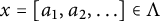
 $x \in \Lambda $
as its symbolic representation
$x \in \Lambda $
as its symbolic representation
 $x = [a_{1}, a_{2}, \ldots ]$
, where
$x = [a_{1}, a_{2}, \ldots ]$
, where
 $G^{j-1}(x) \in J_{a_{j}}$
. In this notation,
$G^{j-1}(x) \in J_{a_{j}}$
. In this notation,
 $\varphi $
above can be written as
$\varphi $
above can be written as
 $[1, 1, 1, \ldots ]$
. By (iii), we have
$[1, 1, 1, \ldots ]$
. By (iii), we have
 $\varphi < s_{1}$
, from which it is straightforward to check that we indeed have
$\varphi < s_{1}$
, from which it is straightforward to check that we indeed have
 $\delta _{G}(N)>0$
in (iv). For convenience, for
$\delta _{G}(N)>0$
in (iv). For convenience, for
 $j \in \mathbb {Z}^{+}$
, we will denote
$j \in \mathbb {Z}^{+}$
, we will denote
 $\eta _{j}: \Lambda \to \Lambda $
,
$\eta _{j}: \Lambda \to \Lambda $
,
 $\eta _{j} = G^{j-1}$
, so that
$\eta _{j} = G^{j-1}$
, so that
 $$ \begin{align*}\eta_{j}([a_{1}, a_{2}, \ldots]) = [a_{j}, a_{j+1}, \ldots].\end{align*} $$
Henceforth, we will assume that G is restricted to
 $\Lambda $
.
$\Lambda $
.
Now, let
 $u: (s_{0}, s_{1}) \to \mathbb {R}^{+}$
be a
$u: (s_{0}, s_{1}) \to \mathbb {R}^{+}$
be a
 $\mathcal {C}^{1}$
function satisfying the following:
$\mathcal {C}^{1}$
function satisfying the following:
-
(i)
$\lim _{x \to s_{0}^{+}}u(x) = \infty $
. -
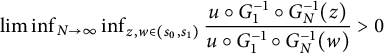
(ii) If
$s_{1}=1$
, then
$\liminf _{N \to \infty } \inf _{z,w \in (s_{0},s_{1})} \dfrac {u \circ G_{1}^{-1} \circ G_{N}^{-1}(z)}{u \circ G_{1}^{-1} \circ G_{N}^{-1}(w)}> 0$
. -
(iii) There is some
$C>0$
such that
$|u'(x)| < \dfrac {C}{(x-s_{0})^{2}}$
for all
$x \in (s_{0}, s_{1})$
. -
(iv) u is computable on numbers
$[a_{1}, a_{2}, \ldots ]$
such that
$a_{l}=1$
for all
$l>l_{0}$
for some integer
$l_{0}$
. -
(v) u is left-computable on all of
$\Lambda $
.


In what follows, for any
 $\nu>0,$
we define the generalized Brjuno function to be
$\nu>0,$
we define the generalized Brjuno function to be
 $$ \begin{align*} \Phi(x) := \sum_{i=1}^{\infty} \left( \eta_{0}(x) \dots \eta_{i-1}(x) \right)^{\nu} \cdot u(\eta_{i}(x)), \end{align*} $$
where
 $x = [a_{1}, a_{2}, \ldots ] \in \Lambda $
.
$x = [a_{1}, a_{2}, \ldots ] \in \Lambda $
.
We note:
Theorem 3.1 The following functions restricted to their corresponding sets
 $\Lambda $
fall under the definition of a generalized Brjuno function given above:
$\Lambda $
fall under the definition of a generalized Brjuno function given above:
-
• Yoccoz’s Brjuno function
${{\mathcal B}}$
(2.1). -
• The first Wilton function
${{\mathcal W}}_{1}$
(2.2). -
• The functions
${{\mathcal B}}_{\alpha , u, \nu }$
(2.5) under the additional assumptions of (ii)–(v) on u. For example, taking
$G = A_{\alpha }$
for
$\alpha \in [1/2,1]$
and
$u(x)$
to be any of
$\log ^{n}(1/x)$
for
$n \in \mathbb {Z}$
or
$x^{-1}$
yields a generalized Brjuno function.


Let us postpone the proof to Section A.1 in the Appendix, and proceed to formulating the results.
3.2 Main results
Theorem 3.2 Let
 $x_*$
be a computable real number in
$x_*$
be a computable real number in
 $\Lambda $
with the property
$\Lambda $
with the property
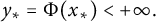 $y_*=\Phi (x_*)<+\infty .$
There exists an oracle TM
$y_*=\Phi (x_*)<+\infty .$
There exists an oracle TM
 $M^\phi $
with a single input
$M^\phi $
with a single input
 $n\in {\mathbb {N}}$
such that the following holds. Suppose
$n\in {\mathbb {N}}$
such that the following holds. Suppose
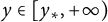
 $y\in [y_*,+\infty )$
and
$y\in [y_*,+\infty )$
and
 $$ \begin{align*}\phi(n)=y_{n}\nearrow y.\end{align*} $$
Then,
 $M^\phi $
outputs
$M^\phi $
outputs
 $d_n$
such that
$d_n$
such that
 $$ \begin{align*}|d_n-x|<2^{-n}\text{ for }x \in \Lambda\text{ such that }\Phi(x)=y.\end{align*} $$
As a corollary:
Corollary 3.3 If
 $y\in [y_*,+\infty )$
is left computable, then there exists a computable
$y\in [y_*,+\infty )$
is left computable, then there exists a computable
 $x\in \Lambda $
with
$x\in \Lambda $
with
 $$ \begin{align*}\Phi(x)=y.\end{align*} $$
In fact, it is clear from the proof of Theorem 3.2 that countably many such
 $x \in \Lambda $
exist.
$x \in \Lambda $
exist.
As was shown in [Reference Balazard and MartinBM12], the Brjuno function
 ${{\mathcal B}}$
attains its global maximum at
${{\mathcal B}}$
attains its global maximum at
 $$ \begin{align*}w_*=\frac{\sqrt{5}-1}{2}=[1,1,1,\ldots].\end{align*} $$
Therefore:
Corollary 3.4 If
 $y\in [{{\mathcal B}}(w_*),+\infty )$
is left computable, then there exists a computable
$y\in [{{\mathcal B}}(w_*),+\infty )$
is left computable, then there exists a computable
 $x\in (0,1)$
with
$x\in (0,1)$
with
 $$ \begin{align*}{{\mathcal B}}(x)=y.\end{align*} $$
4 Proof of Theorem 3.2
4.1 Three main lemmas
It will be helpful to first outline the general strategy for the proof of Theorem 3.2. We are given a computable sequence
 $\{y_{n}\}$
converging upward to some left-computable y, and we must find a computable
$\{y_{n}\}$
converging upward to some left-computable y, and we must find a computable
 $x \in (s_{0}, s_{1})$
for which
$x \in (s_{0}, s_{1})$
for which
 $y = \Phi (x)$
. This is done by starting with some
$y = \Phi (x)$
. This is done by starting with some
 $\gamma _{0} \in (s_{0}, s_{1})$
and iteratively modifying the symbolic representation of
$\gamma _{0} \in (s_{0}, s_{1})$
and iteratively modifying the symbolic representation of
 $\gamma _{k}$
to “squeeze”
$\gamma _{k}$
to “squeeze”
 $\Phi (\gamma _{k})$
to be in the interval
$\Phi (\gamma _{k})$
to be in the interval
 $(\Phi (\gamma _{s+k})-2^{-k}\varepsilon , \Phi (\gamma _{s+k})+2^{-k}\varepsilon )$
for some positive integer s. Passing to the limit, we obtain
$(\Phi (\gamma _{s+k})-2^{-k}\varepsilon , \Phi (\gamma _{s+k})+2^{-k}\varepsilon )$
for some positive integer s. Passing to the limit, we obtain
 $x = \gamma _{\infty }$
for which
$x = \gamma _{\infty }$
for which
 $\Phi (x) = y$
as needed.
$\Phi (x) = y$
as needed.
To ensure this strategy works, we need ways of carefully controlling the value of
 $\Phi (\gamma )$
from the symbolic representation of
$\Phi (\gamma )$
from the symbolic representation of
 $\gamma $
. This role is played by Lemmas 4.1–4.3 below, which are analogous to Lemmas 5.18–5.20, respectively, in [Reference Braverman and YampolskyBY09] and whose proofs are in the Section A.2 in the Appendix.
$\gamma $
. This role is played by Lemmas 4.1–4.3 below, which are analogous to Lemmas 5.18–5.20, respectively, in [Reference Braverman and YampolskyBY09] and whose proofs are in the Section A.2 in the Appendix.
Lemma 4.1 For any initial segment
 $I = [a_{1}, a_{2}, \ldots , a_{n}]$
, write
$I = [a_{1}, a_{2}, \ldots , a_{n}]$
, write
 $\omega = [a_{1}, a_{2}, \ldots , a_{n}, 1, 1, 1, \ldots ]$
. Then, for any
$\omega = [a_{1}, a_{2}, \ldots , a_{n}, 1, 1, 1, \ldots ]$
. Then, for any
 $\varepsilon> 0$
, there is an
$\varepsilon> 0$
, there is an
 $m> 0$
and an integer N such that if we write
$m> 0$
and an integer N such that if we write
 $\beta ^{N} = [a_{1}, a_{2}, \ldots , a_{n}, 1, 1, \ldots , 1, N, 1, 1, \ldots ]$
, where the N is located in the
$\beta ^{N} = [a_{1}, a_{2}, \ldots , a_{n}, 1, 1, \ldots , 1, N, 1, 1, \ldots ]$
, where the N is located in the
 $(n+m)$
-th position, then
$(n+m)$
-th position, then
 $$ \begin{align*} \Phi(\omega) + \varepsilon < \Phi(\beta^{N}) < \Phi(\omega) + 2 \varepsilon. \end{align*} $$
In the Appendix, this lemma will be proven under the slightly weaker assumptions used in Section 5. Also, it is clear from the proof that m can be taken arbitrarily large.
Lemma 4.2 With
 $\omega $
as above, for any
$\omega $
as above, for any
 $\varepsilon>0,$
there is an
$\varepsilon>0,$
there is an
 $m_{0}>0$
, which can be computed from
$m_{0}>0$
, which can be computed from
 $(a_{0}, a_{1}, \ldots , a_{n})$
and
$(a_{0}, a_{1}, \ldots , a_{n})$
and
 $\varepsilon $
, such that for any
$\varepsilon $
, such that for any
 $m \geq m_{0}$
and any tail
$m \geq m_{0}$
and any tail
 $I = [a_{n+m}, a_{n+m+1}, \ldots ],$
we have
$I = [a_{n+m}, a_{n+m+1}, \ldots ],$
we have
 $$ \begin{align*} \Phi(\beta^{I})> \Phi(\omega) - \varepsilon, \end{align*} $$
where
 $$ \begin{align*} \beta^{I} = [a_{1}, a_{2}, \ldots, a_{n}, 1, 1, \ldots, 1, a_{n+m}, a_{n+m+1}, \ldots]. \end{align*} $$
Lemma 4.3 Let
 $\omega = [a_{1}, a_{2}, \ldots ]$
be such that
$\omega = [a_{1}, a_{2}, \ldots ]$
be such that
 $\Phi (\omega ) < \infty $
. Write
$\Phi (\omega ) < \infty $
. Write
 $\omega _{k} = [a_{1}, a_{2}, \ldots , a_{k}, 1, 1, \ldots ]$
. Then, for every
$\omega _{k} = [a_{1}, a_{2}, \ldots , a_{k}, 1, 1, \ldots ]$
. Then, for every
 $\varepsilon>0,$
there is an m such that for all
$\varepsilon>0,$
there is an m such that for all
 $k \geq m$
,
$k \geq m$
,
 $$ \begin{align*} \Phi(\omega_{k}) < \Phi(\omega) + \varepsilon. \end{align*} $$
We proceed with proving Theorem 3.2.
4.2 The proof
We first require a few preliminary results.
Proposition 4.4 Let
 $m_{0}>0$
be an integer. Then, there exists an oracle TM which, given access to a number
$m_{0}>0$
be an integer. Then, there exists an oracle TM which, given access to a number
 $x = [a_{1}, a_{2}, \ldots ] \in \Lambda $
such that
$x = [a_{1}, a_{2}, \ldots ] \in \Lambda $
such that
 $a_{m} = 1$
for
$a_{m} = 1$
for
 $m>m_{0}$
, computes
$m>m_{0}$
, computes
 $\Phi (x)$
.
$\Phi (x)$
.
Proof Let
 $\varphi = [1, 1, 1, \ldots ]$
. For any
$\varphi = [1, 1, 1, \ldots ]$
. For any
 $x,$
we have
$x,$
we have
 $$ \begin{align*} \Phi(x) &= \sum_{i=1}^{m_{0}} \left( \eta_{0}(x) \dots \eta_{i-1}(x) \right)^{\nu} \cdot u(\eta_{i}(x)) + \sum_{i=m_{0}+1}^{\infty} \left( \varphi^{\nu} \right)^{n-1} \cdot u(\varphi) \\ &= \sum_{i=1}^{m_{0}} \left( \eta_{0}(x) \dots \eta_{i-1}(x) \right)^{\nu} \cdot u(\eta_{i}(x)) + \frac{\varphi^{\nu \cdot m_{0}}}{1-\varphi^{\nu}} \cdot u(\varphi). \end{align*} $$
Since u is computable on each number
 $\eta _{i}(x)$
whose symbolic representation ends in all ones by assumption (iv) on u, and each
$\eta _{i}(x)$
whose symbolic representation ends in all ones by assumption (iv) on u, and each
 $\eta _{j}$
is computable on all of
$\eta _{j}$
is computable on all of
 $\Lambda $
by assumption (vi) on G, there is an oracle TM which, given access to x, computes the sum on the left to an arbitrary precision. The construction of this oracle TM is independent of x and depends only on
$\Lambda $
by assumption (vi) on G, there is an oracle TM which, given access to x, computes the sum on the left to an arbitrary precision. The construction of this oracle TM is independent of x and depends only on
 $m_{0}$
. Additionally, since
$m_{0}$
. Additionally, since
 $\varphi $
also ends in all ones, there is a TM which computes the value of the term on the right to an arbitrary precision, also depending only on
$\varphi $
also ends in all ones, there is a TM which computes the value of the term on the right to an arbitrary precision, also depending only on
 $m_{0}$
. Combining these TMs in the obvious way, we obtain an oracle TM which, given access to x, computes
$m_{0}$
. Combining these TMs in the obvious way, we obtain an oracle TM which, given access to x, computes
 $\Phi (x)$
to an arbitrary precision.
$\Phi (x)$
to an arbitrary precision.
Lemma 4.5 Given an initial segment
 $I = [a_{0}, a_{1}, \ldots , a_{n}]$
and
$I = [a_{0}, a_{1}, \ldots , a_{n}]$
and
 $m_{0}>0$
, write
$m_{0}>0$
, write
 $\omega = [a_{0}, a_{1}, \ldots , a_{n}, 1, 1, \ldots ]$
. Then, for all
$\omega = [a_{0}, a_{1}, \ldots , a_{n}, 1, 1, \ldots ]$
. Then, for all
 $\varepsilon>0$
, we can uniformly compute
$\varepsilon>0$
, we can uniformly compute
 $m>m_{0}$
and
$m>m_{0}$
and
 $t, N \in \mathbb {Z}^{+}$
such that if we write
$t, N \in \mathbb {Z}^{+}$
such that if we write
 $\beta = [a_{0}, a_{1}, \ldots , a_{n}, 1, 1, \ldots , 1, N , 1, 1, \ldots ]$
, where N is in the
$\beta = [a_{0}, a_{1}, \ldots , a_{n}, 1, 1, \ldots , 1, N , 1, 1, \ldots ]$
, where N is in the
 $(n+m)$
-th position, we have
$(n+m)$
-th position, we have
 $$ \begin{align} \Phi(\omega) + \varepsilon < \Phi(\beta) < \Phi(\omega) + 2\varepsilon, \end{align} $$
and for any
 $\gamma = [a_{0}, a_{1}, \ldots , a_{n}, 1, 1, \ldots , 1, N , 1, \ldots , 1, c_{n+m+t+1}, c_{n+m+t+2}, \ldots ]$
, we have
$\gamma = [a_{0}, a_{1}, \ldots , a_{n}, 1, 1, \ldots , 1, N , 1, \ldots , 1, c_{n+m+t+1}, c_{n+m+t+2}, \ldots ]$
, we have
 $$ \begin{align} \Phi(\gamma)> \Phi(\omega) - 2^{-n}. \end{align} $$
Proof We will first show that such
 $m, N$
exist, then give an algorithm to compute them. Let
$m, N$
exist, then give an algorithm to compute them. Let
 $\varepsilon>0$
be given. By Lemma 4.1, there exists m (and we can make
$\varepsilon>0$
be given. By Lemma 4.1, there exists m (and we can make
 $m>m_{0}$
) and
$m>m_{0}$
) and
 $\exists N \in \mathbb {Z}^{+}$
such that
$\exists N \in \mathbb {Z}^{+}$
such that
 $$ \begin{align*} \Phi(\omega) + \varepsilon < \Phi(\beta) < \Phi(\omega) + 2\varepsilon. \end{align*} $$
Taking
 $I'=[a_{0}, a_{1}, \ldots , a_{n}, 1, 1, \ldots , 1, N]$
and
$I'=[a_{0}, a_{1}, \ldots , a_{n}, 1, 1, \ldots , 1, N]$
and
 $\omega '=\beta $
, applying Lemma 4.2 with
$\omega '=\beta $
, applying Lemma 4.2 with
 $\varepsilon '=2^{-n}$
, we get
$\varepsilon '=2^{-n}$
, we get
 $t_{0}>0,$
which can be computed from
$t_{0}>0,$
which can be computed from
 $(a_{0}, a_{1}, \ldots , a_{n}, 1, 1, \ldots , 1, N)$
such that for all
$(a_{0}, a_{1}, \ldots , a_{n}, 1, 1, \ldots , 1, N)$
such that for all
 $t \geq t_{0}$
and any tail
$t \geq t_{0}$
and any tail
 $I = [c_{n+m+t+1}, c_{n+m+t+2}, \ldots ]$
, we have
$I = [c_{n+m+t+1}, c_{n+m+t+2}, \ldots ]$
, we have
 $$ \begin{align*} \Phi(\gamma)> \Phi(\omega') -2^{-n} = \Phi(\beta)-2^{-n} > \Phi(\omega)-2^{-n} \end{align*} $$
as needed.
Since
 $\omega , \beta $
have symbolic representations ending in all ones, for any specific
$\omega , \beta $
have symbolic representations ending in all ones, for any specific
 $m,N,$
we can compute
$m,N,$
we can compute
 $\Phi (\omega )$
and
$\Phi (\omega )$
and
 $\Phi (\beta )$
by Proposition 4.4. So, we can find the required
$\Phi (\beta )$
by Proposition 4.4. So, we can find the required
 $m,N$
by enumerating all pairs
$m,N$
by enumerating all pairs
 $(m,N)$
and exhaustively checking equations (4.1) and (4.2) for each of them. We know that we will eventually find a pair for which these equations hold. Once we have m and N, we can use Lemma 4.2 to compute t.
$(m,N)$
and exhaustively checking equations (4.1) and (4.2) for each of them. We know that we will eventually find a pair for which these equations hold. Once we have m and N, we can use Lemma 4.2 to compute t.
Lemma 4.6 The infimum
 $\Phi (x_{*})$
of
$\Phi (x_{*})$
of
 $\Phi (x)$
over all
$\Phi (x)$
over all
 $x \in \Lambda $
is equal to the infimum over the numbers whose symbolic representations have only finitely many terms that are not
$x \in \Lambda $
is equal to the infimum over the numbers whose symbolic representations have only finitely many terms that are not
 $1$
:
$1$
:
 $$ \begin{align*} \Phi(x_{*}) = \inf_{x=[a_{1},a_{2}, \ldots, a_{k}, 1, 1, \ldots]} \Phi(x). \end{align*} $$
Proof Let
 $\varepsilon>0$
be given. By definition of infimum, there exists
$\varepsilon>0$
be given. By definition of infimum, there exists
 $x=[a_{1}, a_{2}, \ldots ]$
such that
$x=[a_{1}, a_{2}, \ldots ]$
such that
 $$ \begin{align*} \Phi(x) < \Phi(x_{*}) + \frac{\varepsilon}{2}. \end{align*} $$
Write
 $x_{k}=[a_{1}, a_{2}, \ldots , a_{k}, 1, 1, \ldots ]$
. By Lemma 4.3, there exists m such that for
$x_{k}=[a_{1}, a_{2}, \ldots , a_{k}, 1, 1, \ldots ]$
. By Lemma 4.3, there exists m such that for
 $k \geq m$
,
$k \geq m$
,
 $$ \begin{align*} \Phi(x_{k}) < \Phi(x) + \frac{\varepsilon}{2}. \end{align*} $$
Thus,
 $\Phi (x_{k})< \Phi (x_{*}) + \varepsilon $
, so we can make
$\Phi (x_{k})< \Phi (x_{*}) + \varepsilon $
, so we can make
 $\Phi (x_{k})$
as close to
$\Phi (x_{k})$
as close to
 $\Phi (x_{*})$
as we need.
$\Phi (x_{*})$
as we need.
Now, we are given
 $$ \begin{align*} y_{n}\nearrow y, \hspace{15px} y\in[y_*,+\infty). \end{align*} $$
The case of
 $y = y_{*}$
is trivial, so we suppose
$y = y_{*}$
is trivial, so we suppose
 $y> y_{*}$
. Then, there is an s and an
$y> y_{*}$
. Then, there is an s and an
 $\varepsilon>0$
such that
$\varepsilon>0$
such that
 $$ \begin{align*} y_{s}> \Phi(x_{*}) + 2\varepsilon. \end{align*} $$
By Lemma 4.6, there exists
 $\gamma _{0}=[a_{1}, a_{2}, \ldots , a_{n}, 1, 1, \ldots ]$
such that
$\gamma _{0}=[a_{1}, a_{2}, \ldots , a_{n}, 1, 1, \ldots ]$
such that
 $$ \begin{align*} y_{s} - \varepsilon < \Phi(\gamma_{0}) < y_{s} - \frac{\varepsilon}{2}. \end{align*} $$
We will now give an algorithm for computing a number
 $x \in \Lambda $
for which
$x \in \Lambda $
for which
 $\Phi (x) = \lim \nearrow y_{n} = y$
, which would complete the proof of Theorem 3.2. The algorithm works as follows. At state
$\Phi (x) = \lim \nearrow y_{n} = y$
, which would complete the proof of Theorem 3.2. The algorithm works as follows. At state
 $k,$
it produces a finite initial segment
$k,$
it produces a finite initial segment
 $I_{k}=[a_{0}, \ldots , a_{k}]$
such that the following properties hold:
$I_{k}=[a_{0}, \ldots , a_{k}]$
such that the following properties hold:
-
(1)
$I_{0} = [a_{1}, a_{2}, \ldots , a_{n}]$
. -
(2)
$I_{k}$
has at least k terms, i.e.,
$m_{k} \geq k$
. -
(3) For each k,
$I_{k+1}$
is an extension of
$I_{k}$
. -
(4) For each k, define
$\gamma _{k}=[I_{k}, 1, 1, \ldots ]$
. Then,
$$ \begin{align*} y_{s+k} - 2^{-k} \varepsilon < \Phi(\gamma_{k}) < y_{s+k} - 2^{-(k+1)} \varepsilon. \end{align*} $$
-
(5) For each k,
$\Phi (\gamma _{k})> \Phi (\gamma _{k+1})$
. -
(6) For each k and any extension
$\beta = [I_{k}, b_{m_{k}+1}, b_{m_{k}+2}, \ldots ]$
, we have
$$ \begin{align*} \Phi(\beta)> \Phi(\gamma_{k})-2^{-k}. \end{align*} $$


The first three properties are easy to verify. The last three are checked using Lemma 4.5. By this lemma, we can increase
 $\Phi (\gamma _{k-1})$
by any given amount, possibly in more than one step, by extending
$\Phi (\gamma _{k-1})$
by any given amount, possibly in more than one step, by extending
 $I_{k-1}$
to
$I_{k-1}$
to
 $I_{k}$
. Thus, if we have
$I_{k}$
. Thus, if we have
 $$ \begin{align*} y_{s+k-1} -2^{-(k-1)} \varepsilon < \Phi(\gamma_{k-1}) < y_{s+k-1} -2^{-k} \varepsilon, \end{align*} $$
by virtue of
 $\{ a_{s+k} \}_{k=1}^{\infty }$
being non-decreasing, we have both
$\{ a_{s+k} \}_{k=1}^{\infty }$
being non-decreasing, we have both
 $$ \begin{align*} y_{s+k-1} - 2^{-(k-1)} \varepsilon < y_{s+k} - 2^{-k} \varepsilon \hspace{15px} \text{and} \hspace{15px} y_{s+k-1} - 2^{-k} \varepsilon < y_{s+k} - 2^{-(k+1)} \varepsilon. \end{align*} $$
So, we can increase
 $\Phi (\gamma _{k-1})$
by such a fine amount that
$\Phi (\gamma _{k-1})$
by such a fine amount that
 $$ \begin{align*} y_{s+k} -2^{-k} \varepsilon < \Phi(\gamma_{k}) < y_{s+k} -2^{-(k+1)} \varepsilon, \end{align*} $$
satisfying the fourth and fifth properties. In performing this fine increase, we have used the fact that the
 $y_{s+k}$
’s are computable. The last property is satisfied by Lemma 4.5 (4.2).
$y_{s+k}$
’s are computable. The last property is satisfied by Lemma 4.5 (4.2).
Denote
 $$ \begin{align*} x = \lim_{k \to \infty} \gamma_{k}. \end{align*} $$
The symbolic representation of x is the limit of the initial segments
 $I_{k}$
. This algorithm gives us at least one term of the symbolic representation of x per iteration, and hence we would need at most
$I_{k}$
. This algorithm gives us at least one term of the symbolic representation of x per iteration, and hence we would need at most
 $O(n)$
iterations to compute x with precision
$O(n)$
iterations to compute x with precision
 $2^{-n}$
. The initial segment of
$2^{-n}$
. The initial segment of
 $\gamma _{0}$
can also be computed as in the proof of Lemma 4.5. It remains to show that x is the number we are after.
$\gamma _{0}$
can also be computed as in the proof of Lemma 4.5. It remains to show that x is the number we are after.
Lemma 4.7 We have
 $\Phi (x) = y$
.
$\Phi (x) = y$
.
Proof Taking limits on all sides of (4), we get
 $$ \begin{align*} \lim_{k\to\infty} \Phi(\gamma_{k}) = \lim_{k\to\infty} y_{k} = y. \end{align*} $$
It remains to show
 $\lim _{k\to \infty } \Phi (\gamma _{k}) = \Phi (x)$
. As in Proposition 4.4, denote
$\lim _{k\to \infty } \Phi (\gamma _{k}) = \Phi (x)$
. As in Proposition 4.4, denote
 $x = [a_{1}, a_{2}, \ldots ]$
and let
$x = [a_{1}, a_{2}, \ldots ]$
and let
 $\alpha _{k}=[a_{k}, a_{k+1}, \ldots ], \alpha _{0}=1$
. Let
$\alpha _{k}=[a_{k}, a_{k+1}, \ldots ], \alpha _{0}=1$
. Let
 $\varphi = [1, 1, 1, \ldots ]$
, and additionally for any number
$\varphi = [1, 1, 1, \ldots ]$
, and additionally for any number
 $\xi = [b_{1}, b_{2}, \ldots ] \in \Lambda $
denote
$\xi = [b_{1}, b_{2}, \ldots ] \in \Lambda $
denote
 $(\xi )_{k} = [b_{k}, b_{k+1}, \ldots ]$
. We have
$(\xi )_{k} = [b_{k}, b_{k+1}, \ldots ]$
. We have
 $$ \begin{align*} \Phi(x) &= \lim_{k\to\infty} \left( \sum_{n=1}^{m_{k}} \alpha_{0} \alpha_{1} \dots \alpha_{n-1} \cdot u(\alpha_{n}) \right) \\ &\leq \lim_{k\to\infty} \left( \sum_{n=1}^{m_{k}} \alpha_{0} \alpha_{1} \dots \alpha_{n-1} \cdot u(\alpha_{n}) + \sum_{n=m_{k}+1}^{\infty} \varphi^{n-1} \cdot u(\varphi) \right) \\ &= \lim_{k\to\infty} \Phi(\gamma_{k}). \end{align*} $$
Additionally, taking limits on both sides of (6) with
 $\beta = x$
yields
$\beta = x$
yields
 $$ \begin{align*} \lim_{k\to\infty} \Phi(\gamma_{k}) \leq \Phi(x), \end{align*} $$
therefore
 $\lim _{k\to \infty } \Phi (\gamma _{k}) = \Phi (x)$
.
$\lim _{k\to \infty } \Phi (\gamma _{k}) = \Phi (x)$
.
This concludes the proof of Theorem 3.2.
5 Generalized non-computability result
5.1 Modified assumptions
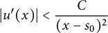
We will now prove a non-computability result about a slightly more broad class of generalized Brjuno functions than the one considered in Section 5. For this result, we require all the assumptions on G except (v) and (vi), and on u we require only assumption (i) together with a slightly weaker variation of assumption (iii):
-
(iii′) There is some
$C>0$
such that
$u'(x) < \dfrac {C}{(x-s_{0})^{2}}$
for all
$x \in (s_{0}, s_{1})$
.


We can additionally allow for more flexibility in the definition of the generalized Brjuno function by adding a “sign” term:
 $$ \begin{align*} \Phi(x) := \sum_{i=1}^{\infty} s(i) \cdot \left( \eta_{0}(x) \dots \eta_{i-1}(x) \right)^{\nu} \cdot u(\eta_{i}(x)), \end{align*} $$
where
 $\nu>0$
as before and
$\nu>0$
as before and
 $s(i) \in \{-1, 1\}$
.
$s(i) \in \{-1, 1\}$
.
Theorem 5.1 The following functions restricted to their corresponding sets
 $\Lambda $
fall under the definition of a generalized Brjuno function given above:
$\Lambda $
fall under the definition of a generalized Brjuno function given above:
-
• Yoccoz’s Brjuno function
${{\mathcal B}}$
(2.1). -
• The first Wilton function
${{\mathcal W}}_{1}$
(2.2) and the second Wilton function
${{\mathcal W}}_{2}$
(2.3). -
• The functions
${{\mathcal B}}_{\alpha , u, \nu }$
(2.5) under the additional assumption of (iii
$'$
) on u. As before, taking
$G = A_{\alpha }$
for
$\alpha \in [1/2,1]$
and
$u(x)$
to be any of
$\log ^{n}(1/x)$
for
$n \in \mathbb {Z}$
or
$x^{-1}$
yields a generalized Brjuno function.


The proof is completely analogous to the proof of Theorem 3.1 and will be omitted.
5.2 Noncomputability result
We proceed with the main result of this section, which concerns the computability of the function
 $\Phi $
as opposed to the computability of real numbers.
$\Phi $
as opposed to the computability of real numbers.
Theorem 5.2 There exists a number
 $x \in \Lambda $
for which
$x \in \Lambda $
for which
 $\Phi (\cdot )$
as defined above is not computable at x.
$\Phi (\cdot )$
as defined above is not computable at x.
Without loss of generality, we will assume in what follows that the sign term
 $s(i) = 1$
infinitely often (otherwise, just replace
$s(i) = 1$
infinitely often (otherwise, just replace
 $\Phi $
with
$\Phi $
with
 $-\Phi $
).
$-\Phi $
).
As before, it will be instructive to first go over the strategy of the proof. This outline is rough and is not fully logically sound, however, it captures the main idea of the argument. To prove a function is non-computable at a single point x, it suffices to enumerate all oracle TMs
 $M^{\phi }_{i}$
,
$M^{\phi }_{i}$
,
 $i \in \mathbb {N}$
(recall that there are countably many oracle TMs), and show that if
$i \in \mathbb {N}$
(recall that there are countably many oracle TMs), and show that if
 $\phi $
is any oracle of
$\phi $
is any oracle of
 $x,$
then
$x,$
then
 $M^{\phi }_{i}$
does not approximate
$M^{\phi }_{i}$
does not approximate
 $\Phi (x)$
arbitrarily well.
$\Phi (x)$
arbitrarily well.
We start with
 $x_{0} = [1, 1, 1, \ldots ]$
and the first TM
$x_{0} = [1, 1, 1, \ldots ]$
and the first TM
 $M^{\phi }_{n_{1}}$
in our enumeration which computes
$M^{\phi }_{n_{1}}$
in our enumeration which computes
 $x_{0}$
. If any of the digits
$x_{0}$
. If any of the digits
 $a_{j}$
in the symbolic representation of
$a_{j}$
in the symbolic representation of
 $x_{0}$
are changed to some
$x_{0}$
are changed to some
 $N \in \mathbb {Z}^{+}$
, as
$N \in \mathbb {Z}^{+}$
, as
 $N \to \infty ,$
the series
$N \to \infty ,$
the series
 $\Phi (x)$
diverges. However, if we change some digit
$\Phi (x)$
diverges. However, if we change some digit
 $a_{j}$
far enough in the representation of
$a_{j}$
far enough in the representation of
 $x_{0}$
, for any
$x_{0}$
, for any
 $N,$
the new value of
$N,$
the new value of
 $x_{0}$
changes by at most some fixed small amount
$x_{0}$
changes by at most some fixed small amount
 $\varepsilon _{j}$
which goes to
$\varepsilon _{j}$
which goes to
 $0$
as
$0$
as
 $j \to \infty $
. So, the idea is to define
$j \to \infty $
. So, the idea is to define
 $x_{1}$
from
$x_{1}$
from
 $x_{0}$
by changing
$x_{0}$
by changing
 $a_{j_{1}}$
for large enough
$a_{j_{1}}$
for large enough
 $j_{1}$
to some large enough
$j_{1}$
to some large enough
 $N_{1}$
, such that if
$N_{1}$
, such that if
 $M^{\phi }_{n_{1}}$
is given an oracle for
$M^{\phi }_{n_{1}}$
is given an oracle for
 $x_{1}$
, then it does not properly compute
$x_{1}$
, then it does not properly compute
 $\Phi (x_{1})$
, which in some sense “fools” the oracle TM
$\Phi (x_{1})$
, which in some sense “fools” the oracle TM
 $M^{\phi }_{n_{1}}$
. To fool the machine
$M^{\phi }_{n_{1}}$
. To fool the machine
 $M^{\phi }_{n_{2}}$
, we then change a digit
$M^{\phi }_{n_{2}}$
, we then change a digit
 $j_{2}>j_{1}$
sufficiently far in the symbolic representation of
$j_{2}>j_{1}$
sufficiently far in the symbolic representation of
 $x_{1}$
to a large
$x_{1}$
to a large
 $N_{2}$
to get
$N_{2}$
to get
 $x_{2}$
, in such a way that neither
$x_{2}$
, in such a way that neither
 $M^{\phi }_{n_{2}}$
nor any other
$M^{\phi }_{n_{2}}$
nor any other
 $M^{\phi }_{k}$
for
$M^{\phi }_{k}$
for
 $k < n_{2}$
properly compute
$k < n_{2}$
properly compute
 $\Phi (x_{2})$
. Continuing in this manner, we will arrive at a limiting number
$\Phi (x_{2})$
. Continuing in this manner, we will arrive at a limiting number
 $x_{\infty } \in \Lambda $
, with
$x_{\infty } \in \Lambda $
, with
 $\Phi (x_{\infty }) < \infty $
and such that none of the oracle TMs
$\Phi (x_{\infty }) < \infty $
and such that none of the oracle TMs
 $M^{\phi }_{i}$
in our list properly compute
$M^{\phi }_{i}$
in our list properly compute
 $x_{\infty }$
.
$x_{\infty }$
.
As in the proof of Theorem 4.3, we will need to carefully control the value of
 $\Phi (x)$
from the symbolic expansion of x. For the proof of Theorem 5.2, we only need Lemma 4.1 from the previous section, which is proven in the Appendix under the weaker assumptions on
$\Phi (x)$
from the symbolic expansion of x. For the proof of Theorem 5.2, we only need Lemma 4.1 from the previous section, which is proven in the Appendix under the weaker assumptions on
 $\Phi $
used in this section.
$\Phi $
used in this section.
For the below proofs, we will say that
 $\Phi (x)$
is computable at x if there exists a TM
$\Phi (x)$
is computable at x if there exists a TM
 $M^{\phi }$
such that if
$M^{\phi }$
such that if
 $\phi $
is an oracle for x, then on input n,
$\phi $
is an oracle for x, then on input n,
 $M^{\phi }$
outputs some
$M^{\phi }$
outputs some
 $y'$
for which
$y'$
for which
 $|\Phi (x)-y'| \leq 2^{-n}$
. This definition uses “
$|\Phi (x)-y'| \leq 2^{-n}$
. This definition uses “
 $\leq $
” instead of the “
$\leq $
” instead of the “
 $<$
” which is used in the definition given in Section 2, but it is easy to see that the two definitions are equivalent.
$<$
” which is used in the definition given in Section 2, but it is easy to see that the two definitions are equivalent.
Before starting the proof, we need the following elementary fact.
Lemma 5.3 Write any number in
 $\Lambda $
as
$\Lambda $
as
 $\omega = [a_{1}, a_{2}, \ldots ]$
. For any
$\omega = [a_{1}, a_{2}, \ldots ]$
. For any
 $\varepsilon> 0$
, there is an
$\varepsilon> 0$
, there is an
 $L>0$
for which
$L>0$
for which
 $n>L$
implies that for any sequence of natural numbers
$n>L$
implies that for any sequence of natural numbers
 $(N_{0}, N_{1}, \ldots )$
,
$(N_{0}, N_{1}, \ldots )$
,
 $$ \begin{align*} |\omega - [a_{1}, a_{2}, \ldots, a_{n-1}, N_{0}, N_{1}, \ldots]| < \varepsilon. \end{align*} $$
Proof Let
 $M>0$
be large enough that
$M>0$
be large enough that
 $\dfrac {s_{1}-s_{0}}{\tau ^{M}} < \varepsilon $
and let
$\dfrac {s_{1}-s_{0}}{\tau ^{M}} < \varepsilon $
and let
 $L = \kappa \cdot M$
, where
$L = \kappa \cdot M$
, where
 $\kappa , \tau $
are from assumption (ii) on G. Noting that
$\kappa , \tau $
are from assumption (ii) on G. Noting that
 $$ \begin{align*} \omega, [a_{1}, a_{2}, \ldots, a_{n-1}, N_{0}, N_{1}] \in (G_{a_{1}}^{-1} \circ G_{a_{2}}^{-1} \circ \cdots \circ G_{a_{n-1}}^{-1})((s_{0}, s_{1})) \end{align*} $$
and
 $|(G_{a_{i+\kappa -1}} \circ G_{a_{i+\kappa -2}} \circ \cdots \circ G_{a_{i}})'(\theta )|> \tau > 1 \implies |(G_{a_{i}}^{-1} \circ G_{a_{i+1}}^{-1} \circ \cdots \circ G_{a_{i+\kappa -1}}^{-1})'(\theta )| < \frac {1}{\tau } < 1$
, as well as
$|(G_{a_{i+\kappa -1}} \circ G_{a_{i+\kappa -2}} \circ \cdots \circ G_{a_{i}})'(\theta )|> \tau > 1 \implies |(G_{a_{i}}^{-1} \circ G_{a_{i+1}}^{-1} \circ \cdots \circ G_{a_{i+\kappa -1}}^{-1})'(\theta )| < \frac {1}{\tau } < 1$
, as well as
 $|(G_{a_{i}}^{1})'(\theta )| < 1$
from (ii), we have
$|(G_{a_{i}}^{1})'(\theta )| < 1$
from (ii), we have
 $$ \begin{align*} &\text{length}((G_{a_{1}}^{-1} \circ \cdots \circ G_{a_{n-1}}^{-1})((s_{0}, s_{1}))) \\ &\quad \leq \left( \prod_{i=0}^{M-1} \sup_{\theta \in \Lambda} |(G_{a_{i\kappa+1}}^{-1} \circ \cdots \circ G_{a_{i\kappa+\kappa}}^{-1})'(\theta)| \right) \cdot \left( \prod_{j=L+1}^{n-1} \sup_{\theta \in \Lambda} |(G_{a_{j}}^{-1})'(\theta)| \right) \cdot (s_{1} - s_{0}) \\ &\quad < \dfrac{s_{1}-s_{0}}{\tau^{M}} < \varepsilon. \end{align*} $$
In particular, we have the following.
Corollary 5.4 For
 $\omega = [a_{1}, a_{2}, \ldots ]$
as above, for any
$\omega = [a_{1}, a_{2}, \ldots ]$
as above, for any
 $\varepsilon> 0$
, there is an
$\varepsilon> 0$
, there is an
 $L>0$
for which
$L>0$
for which
 $n>L$
implies that
$n>L$
implies that
 $\forall N \in \mathbb {N}$
,
$\forall N \in \mathbb {N}$
,
 $$ \begin{align*} |\omega - [a_{1}, a_{2}, \ldots, a_{n-1}, N, a_{n+1}, \ldots]| < \varepsilon. \end{align*} $$
Before proceeding to the proof of the main result, we first define some notation. For any
 $x_{i} = [a_{1}^{i}, a_{2}^{i}, \ldots ],$
let
$x_{i} = [a_{1}^{i}, a_{2}^{i}, \ldots ],$
let
 $\eta _{k}^{i}=[a_{k}^{i}, a_{k+1}^{i}, \ldots ]$
, noting that
$\eta _{k}^{i}=[a_{k}^{i}, a_{k+1}^{i}, \ldots ]$
, noting that
 $$ \begin{align*} \Phi(x_{i})=\sum_{n=1}^{\infty} s(i) \cdot \left( \eta_{0}^{i} \eta_{1}^{i} \dots \eta_{n-1}^{i} \right)^{\nu} \cdot u(\eta_{n}^{i}), \end{align*} $$
where
 $\nu , \rho>0$
and
$\nu , \rho>0$
and
 $s(i) \in \{-1, 1\}$
with
$s(i) \in \{-1, 1\}$
with
 $s(i) = 1$
infinitely often. Let
$s(i) = 1$
infinitely often. Let
 $$ \begin{align*} f(i,k)=\sum_{n=1}^{k}s(i) \cdot \left( \eta_{0}^{i} \eta_{1}^{i} \dots \eta_{n-1}^{i} \right)^{\nu} \cdot u(\eta_{n}^{i}), \end{align*} $$
noting that
 $\lim _{k \to \infty }f(i, k) = \Phi (x_{i})$
.
$\lim _{k \to \infty }f(i, k) = \Phi (x_{i})$
.
5.3 Proof of Theorem 5.2
We will first show inductively that there exist:
-
• nested initial segments
$I_{1} \subseteq I_{2} \subseteq \dots $
, where each
$I_{i}$
has length
$p_{i}$
; -
• for each
$i = 1, 2, \ldots $
, positive integers
$N^{i}$
and
$m_{i}$
; -
• positive integers
$k_{1} < k_{2} < \cdots $
and
$l_{1} < l_{2} < \cdots $
and
$\hat {a}_{1} < \hat {a}_{2} < \cdots $
and
$n(0) < n(1) < n(2) < \cdots $
, positive real numbers
$\hat {\varepsilon }_{1}> \hat {\varepsilon }_{2} > \cdots $
, and oracles
$\phi _{0}, \phi _{1}, \ldots $
;


such that if we let
 $x_{i} = [I_{i}, 1, \ldots , 1, N^{i}, 1, \ldots ]$
for
$x_{i} = [I_{i}, 1, \ldots , 1, N^{i}, 1, \ldots ]$
for
 $i \in \mathbb {Z}^{+}$
, where
$i \in \mathbb {Z}^{+}$
, where
 $N^{i}$
is in the
$N^{i}$
is in the
 $(m_{i}+p_{i})$
-th position, then we have the following:
$(m_{i}+p_{i})$
-th position, then we have the following:
-
(1)
$\phi _{i}$
is an oracle for
$x_{i}$
such that
$|\phi _{i}(n) - x_{i}| < 2^{-(n+1)}$
for all n. -
(2)
$\phi _{i}$
agrees with the oracle
$\phi _{j-1}$
on inputs
$1, 2, \ldots , k_{j}$
for
$j=1, 2, \ldots , i$
. -
(3) Running
$M_{l_{i}}^{\phi _{i}}(1), M_{l_{i}}^{\phi _{i}}(2), \ldots , M_{l_{i}}^{\phi _{i}}(\hat {a}_{i})$
queries
$\phi _{i}$
with parameters not exceeding
$k_{i}$
. -
(4) Running
$M_{l_{i}}^{\phi _{i}}(\hat {a}_{i})$
yields a number
$A_{l_{i}}$
for which
$$ \begin{align*} A_{l_{i}} + 2^{-\hat{a}_{i}} \leq \Phi(x_{i-1}) + 2^{-\hat{a}_{i}+1} < \Phi(x_{i}) < \Phi(x_{i-1}) + 2 \cdot 2^{-\hat{a}_{i}+1}. \end{align*} $$
-
(5) Running
$M_{l_{j}}^{\phi _{i}}(\hat {a}_{j})$
for
$j = 1, 2, \ldots , i$
yields a number
$B_{l_{j}}$
for which
$B_{l_{j}} + 2^{-\hat {a}_{j}} < \Phi (x_{i})$
. -
(6) The TMs
$M^{\phi _{i}}_{k}$
for
$k \in \{1, \ldots , l_{i}\}$
all do not properly compute
$\Phi (x_{i})$
; in particular, they all compute
$\Phi (x_{i})$
with an error of at least
$\hat {\varepsilon }_{i}$
. -
(7) For
$k\geq n(i)$
, we have
$|f(i,k)-\Phi (x_{i})| < 2^{-i}$
. -
(8) For
$k = 1, 2, \ldots , n(i-1)$
, we have
$|f(i,k)-f(i-1,k)|<2^{-i}$
.


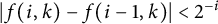
5.3.1 Base case
There are countably many oracle TMs
 $M^{\phi }$
, where
$M^{\phi }$
, where
 $\phi $
represents an oracle for x, so we can order them as
$\phi $
represents an oracle for x, so we can order them as
 $M_{1}^{\phi }, M_{2}^{\phi }, \ldots $
. Let
$M_{1}^{\phi }, M_{2}^{\phi }, \ldots $
. Let
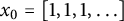 $x_{0} = [1, 1, 1, \ldots ]$
. Given an oracle
$x_{0} = [1, 1, 1, \ldots ]$
. Given an oracle
 $\phi _{0}$
for
$\phi _{0}$
for
 $x_{0}$
such that
$x_{0}$
such that
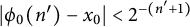 $|\phi _{0}(n') - x_{0}| < 2^{-(n'+1)}$
for all
$|\phi _{0}(n') - x_{0}| < 2^{-(n'+1)}$
for all
 $n'$
, let
$n'$
, let
 $M_{l_{1}}^{\phi _{0}}$
be the first TM to compute
$M_{l_{1}}^{\phi _{0}}$
be the first TM to compute
 $\Phi (x_{0})$
(if no such TM exists, we are done). Since this is the first such TM, all of
$\Phi (x_{0})$
(if no such TM exists, we are done). Since this is the first such TM, all of
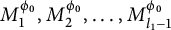 $M_{1}^{\phi _{0}}, M_{2}^{\phi _{0}}, \ldots , M_{l_{1}-1}^{\phi _{0}}$
do not properly compute
$M_{1}^{\phi _{0}}, M_{2}^{\phi _{0}}, \ldots , M_{l_{1}-1}^{\phi _{0}}$
do not properly compute
 $\Phi (x_{0})$
, so there are integers
$\Phi (x_{0})$
, so there are integers
 $a_{1}, a_{2}, \ldots , a_{l_{1}-1}$
and small positive real numbers
$a_{1}, a_{2}, \ldots , a_{l_{1}-1}$
and small positive real numbers
 $\varepsilon _{1}, \varepsilon _{2}, \ldots , \varepsilon _{l_{1}-1}$
for which
$\varepsilon _{1}, \varepsilon _{2}, \ldots , \varepsilon _{l_{1}-1}$
for which
 $M_{k}^{\phi _{0}}(a_{k})$
outputs some number
$M_{k}^{\phi _{0}}(a_{k})$
outputs some number
 $A_{k}$
with
$A_{k}$
with
 $|A_{k} - \Phi (x_{0})|> 2^{-a_{k}} + \varepsilon _{k}$
. Set
$|A_{k} - \Phi (x_{0})|> 2^{-a_{k}} + \varepsilon _{k}$
. Set
 $\hat {\varepsilon }_{1} = \min (\varepsilon _{1}, \ldots , \varepsilon _{l_{1}-1})$
; choose
$\hat {\varepsilon }_{1} = \min (\varepsilon _{1}, \ldots , \varepsilon _{l_{1}-1})$
; choose
 $\hat {n}_{1}$
large enough so that
$\hat {n}_{1}$
large enough so that
 $2^{-\hat {n}_{1}+2} < \hat {\varepsilon }_{1}/2$
, and set
$2^{-\hat {n}_{1}+2} < \hat {\varepsilon }_{1}/2$
, and set
 $\hat {a}_{1} = \max (a_{1}, \ldots , a_{l_{1}-1}, \hat {n}_{1})$
.
$\hat {a}_{1} = \max (a_{1}, \ldots , a_{l_{1}-1}, \hat {n}_{1})$
.
Run
 $M_{l_{1}}^{\phi _{0}}(\hat {a}_{1})$
with the oracle
$M_{l_{1}}^{\phi _{0}}(\hat {a}_{1})$
with the oracle
 $\phi _{0}$
. This TM outputs a number
$\phi _{0}$
. This TM outputs a number
 $A_{l_{1}}$
for which
$A_{l_{1}}$
for which
 $|A_{l_{1}} - \Phi (x_{0})| \leq 2^{-\hat {a}_{1}}$
. Since the computation is performed in finite time, there is a
$|A_{l_{1}} - \Phi (x_{0})| \leq 2^{-\hat {a}_{1}}$
. Since the computation is performed in finite time, there is a
 $k_{1}>0$
such that
$k_{1}>0$
such that
 $\phi _{0}$
is only queried with parameters not exceeding
$\phi _{0}$
is only queried with parameters not exceeding
 $k_{1}$
. We assume
$k_{1}$
. We assume
 $k_{1}$
is large enough that the computations
$k_{1}$
is large enough that the computations
 $M_{l_{1}}^{\phi _{0}}(k)$
query
$M_{l_{1}}^{\phi _{0}}(k)$
query
 $\phi _{0}$
for parameters not exceeding
$\phi _{0}$
for parameters not exceeding
 $k_{1}$
for
$k_{1}$
for
 $k = 1, 2, \ldots , \hat {a}_{1}-1$
. Setting
$k = 1, 2, \ldots , \hat {a}_{1}-1$
. Setting
 $n(0) = 1$
, we additionally make
$n(0) = 1$
, we additionally make
 $k_{1}$
large enough such that for any
$k_{1}$
large enough such that for any
 $x_{1}$
with
$x_{1}$
with
 $|x_{1} - x_{0}| < 2^{-(k_{1}+1)}$
, we have
$|x_{1} - x_{0}| < 2^{-(k_{1}+1)}$
, we have
 $$ \begin{align*} |f(1, 1)-f(0, 1)| = \left| u(\eta_{1}^{1}) - u(\eta_{1}^{0}) \right| = \left| u(x_{1}) - u(x_{0}) \right| < 2^{-1} \end{align*} $$
by continuity of
 $u(\cdot )$
. Hence, (8) is satisfied.
$u(\cdot )$
. Hence, (8) is satisfied.
Now, for any
 $x_{1}$
such that
$x_{1}$
such that
 $|x_{1} - x_{0}| < 2^{-(k_{1}+1)}$
,
$|x_{1} - x_{0}| < 2^{-(k_{1}+1)}$
,
 $\phi _{0}$
is a valid oracle for
$\phi _{0}$
is a valid oracle for
 $x_{1}$
up to parameter value
$x_{1}$
up to parameter value
 $k_{1}$
. In particular, we can create an oracle
$k_{1}$
. In particular, we can create an oracle
 $\psi $
for
$\psi $
for
 $x_{1}$
which agrees with
$x_{1}$
which agrees with
 $\phi _{0}$
on
$\phi _{0}$
on
 $1, 2, \ldots , k_{1}$
. Then, the execution of
$1, 2, \ldots , k_{1}$
. Then, the execution of
 $M_{l_{1}}^{\phi _{0}}(\hat {a}_{1})$
will be identical to that of
$M_{l_{1}}^{\phi _{0}}(\hat {a}_{1})$
will be identical to that of
 $M_{l_{1}}^{\psi }(\hat {a}_{1})$
, so it will output the same value
$M_{l_{1}}^{\psi }(\hat {a}_{1})$
, so it will output the same value
 $A_{l_{1}}$
which is a
$A_{l_{1}}$
which is a
 $2^{-\hat {a}_{1}}$
-approximation for
$2^{-\hat {a}_{1}}$
-approximation for
 $\Phi (x_{0})$
.
$\Phi (x_{0})$
.
Applying Corollary 5.4 with
 $\varepsilon = 2^{-(k_{1} +1)}$
, we get
$\varepsilon = 2^{-(k_{1} +1)}$
, we get
 $L_{1}>0$
such that
$L_{1}>0$
such that
 $$ \begin{align*} \forall m_{1}>L_{1}, \forall N_{1} \in \mathbb{N}, |\beta^{N_{1}} - x_{0}| < 2^{-(k_{1}+1)}, \end{align*} $$
where
 $\beta ^{N_{1}}$
has all ones except an
$\beta ^{N_{1}}$
has all ones except an
 $N_{1}$
at the
$N_{1}$
at the
 $(m_{1}+1)$
-th position. Applying Lemma 4.1 with
$(m_{1}+1)$
-th position. Applying Lemma 4.1 with
 $I_{1} = [1]$
and
$I_{1} = [1]$
and
 $\varepsilon = 2^{-\hat {a}_{1}+1}$
, and making sure the integer
$\varepsilon = 2^{-\hat {a}_{1}+1}$
, and making sure the integer
 $m=m_{1}$
we get from this lemma satisfies
$m=m_{1}$
we get from this lemma satisfies
 $m_{1}>L_{1}$
, we get some
$m_{1}>L_{1}$
, we get some
 $\beta ^{N_{1}} = \beta _{1}^{N_{1}}$
for which
$\beta ^{N_{1}} = \beta _{1}^{N_{1}}$
for which
 $$ \begin{align*} \exists N_{1} \in \mathbb{N} \text{ such that } |\beta_{1}^{N_{1}} - x_{0}| < 2^{-(k_{1}+1)} \hspace{10px} [\text{since } m_{1}>L_{1}] \end{align*} $$
yet
 $$ \begin{align*} \Phi(x_{0}) + 2^{-\hat{a}_{1}+1} < \Phi(\beta_{1}^{N_{1}}) < \Phi(x_{0}) + 2 \cdot 2^{-\hat{a}_{1}+1}, \end{align*} $$
where
 $\beta _{1}^{N_{1}}$
has all ones except an
$\beta _{1}^{N_{1}}$
has all ones except an
 $N_{1}$
at the
$N_{1}$
at the
 $(m_{1}+1)$
-th position. Let
$(m_{1}+1)$
-th position. Let
 $x_{1} = \beta _{1}^{N_{1}}$
, and let
$x_{1} = \beta _{1}^{N_{1}}$
, and let
 $\phi _{1} = \psi $
be the oracle for
$\phi _{1} = \psi $
be the oracle for
 $x_{1}$
which agrees with
$x_{1}$
which agrees with
 $\phi _{0}$
on
$\phi _{0}$
on
 $1, 2, \ldots , k_{1}$
and which additionally satisfies
$1, 2, \ldots , k_{1}$
and which additionally satisfies
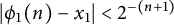 $|\phi _{1}(n)-x_{1}|<2^{-(n+1)}$
for all n. This oracle
$|\phi _{1}(n)-x_{1}|<2^{-(n+1)}$
for all n. This oracle
 $\phi _{1}$
satisfies (1) and (2). As previously stated, the execution of
$\phi _{1}$
satisfies (1) and (2). As previously stated, the execution of
 $M_{l_{1}}^{\phi _{0}}(\hat {a}_{1})$
is identical to that of
$M_{l_{1}}^{\phi _{0}}(\hat {a}_{1})$
is identical to that of
 $M_{l_{1}}^{\phi _{1}}(\hat {a}_{1})$
, so the output will be the same number
$M_{l_{1}}^{\phi _{1}}(\hat {a}_{1})$
, so the output will be the same number
 $A_{l_{1}}$
such that
$A_{l_{1}}$
such that
 $|A_{l_{1}} - \Phi (x_{0})| \leq 2^{-\hat {a}_{1}}$
. By construction,
$|A_{l_{1}} - \Phi (x_{0})| \leq 2^{-\hat {a}_{1}}$
. By construction,
 $M_{l_{1}}^{\phi _{1}}(1), M_{l_{1}}^{\phi _{1}}(2), \ldots , M_{l_{1}}^{\phi _{1}}(\hat {a}_{1})$
only query
$M_{l_{1}}^{\phi _{1}}(1), M_{l_{1}}^{\phi _{1}}(2), \ldots , M_{l_{1}}^{\phi _{1}}(\hat {a}_{1})$
only query
 $\phi _{1}$
with parameters not exceeding
$\phi _{1}$
with parameters not exceeding
 $k_{1}$
, satisfying (3). But then, by the above work,
$k_{1}$
, satisfying (3). But then, by the above work,
 $$ \begin{align*} A_{l_{1}} + 2^{-\hat{a}_{1}} \leq \Phi(x_{0}) + 2^{-\hat{a}_{1}} + 2^{-\hat{a}_{1}} = \Phi(x_{0}) + 2^{-\hat{a}_{1}+1} < \Phi(x_{1}), \end{align*} $$
satisfying (4) and also (5) by taking
 $B_{l_{1}} = A_{l_{1}}$
. Thus,
$B_{l_{1}} = A_{l_{1}}$
. Thus,
 $M_{l_{1}}^{\phi _{1}}(\hat {a}_{1})$
, where
$M_{l_{1}}^{\phi _{1}}(\hat {a}_{1})$
, where
 $\phi _{1}$
is an oracle for
$\phi _{1}$
is an oracle for
 $x_{1}$
, does not approximate
$x_{1}$
, does not approximate
 $\Phi (x_{1})$
with precision
$\Phi (x_{1})$
with precision
 $2^{-\hat {a}_{1}}$
, so this TM does not properly compute this number. Additionally, note that
$2^{-\hat {a}_{1}}$
, so this TM does not properly compute this number. Additionally, note that
 $M_{k}^{\phi _{1}}$
also does not compute
$M_{k}^{\phi _{1}}$
also does not compute
 $\Phi (x_{1})$
for
$\Phi (x_{1})$
for
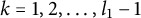 $k = 1, 2, \ldots , l_{1}-1$
. Running
$k = 1, 2, \ldots , l_{1}-1$
. Running
 $M_{k}^{\phi _{1}}(a_{k})$
is identical to running
$M_{k}^{\phi _{1}}(a_{k})$
is identical to running
 $M_{k}^{\phi _{0}}(a_{k})$
by our choice of
$M_{k}^{\phi _{0}}(a_{k})$
by our choice of
 $k_{1}$
in the construction of
$k_{1}$
in the construction of
 $\phi _{1}$
, so
$\phi _{1}$
, so
 $M_{k}^{\phi _{1}}(a_k)$
outputs a number
$M_{k}^{\phi _{1}}(a_k)$
outputs a number
 $B_{k}$
for which
$B_{k}$
for which
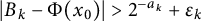 $|B_{k} - \Phi (x_{0})|> 2^{-a_{k}} + \varepsilon _{k}$
. Since
$|B_{k} - \Phi (x_{0})|> 2^{-a_{k}} + \varepsilon _{k}$
. Since
 $$ \begin{align*} |\Phi(x_{1})-\Phi(x_{0})| < 2^{-\hat{a}_{1}+2} < \frac{\hat{\varepsilon}_{1}}{2} \leq \frac{\varepsilon_{k}}{2}, \end{align*} $$
we have
 $$ \begin{align*} |B_{k}-\Phi(x_{1})| &\geq |B_{k}-\Phi(x_{0})| - |\Phi(x_{0})-\Phi(x_{1})|> (2^{-a_{k}} + \varepsilon_{k}) - \frac{\varepsilon_{k}}{2} \\ &= 2^{-a_{k}} + \frac{\varepsilon_{k}}{2} > 2^{-a_{k}}, \end{align*} $$
satisfying (6). To show (7), note that
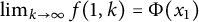 $\lim _{k \to \infty }f(1,k) = \Phi (x_{1})$
is finite, so there is some large enough
$\lim _{k \to \infty }f(1,k) = \Phi (x_{1})$
is finite, so there is some large enough
 $n(1)$
for which
$n(1)$
for which
 $k \geq n(1)$
implies
$k \geq n(1)$
implies
 $|f(1, k) - \Phi (x_{1})| < 2^{-1}$
as required.
$|f(1, k) - \Phi (x_{1})| < 2^{-1}$
as required.
5.3.2 Induction step
Now, inductively, suppose there exist the following:
-
• nested initial segments
$I_{1} \subseteq \dots \subseteq I_{i-1}$
, where each
$I_{j}$
has length
$p_{j}$
; -
• for each
$j = 1, 2, \ldots , i-1$
, positive integers
$N^{j}$
and
$m_{j}$
; -
• positive integers
$k_{1} < k_{2} < \cdots < k_{i-1}$
and
$l_{1} < l_{2} < \cdots < l_{i-1}$
and
$\hat {a}_{1} < \hat {a}_{2} < \cdots < \hat {a}_{i-1}$
and
$n(0) < n(1) < \cdots < n(i-1)$
, positive real numbers
$\hat {\varepsilon }_{1}> \hat {\varepsilon }_{2} > \cdots > \hat {\varepsilon }_{i-1}$
, and oracles
$\phi _{0}, \phi _{1}, \ldots , \phi _{i-1}$
;


such that if we let
 $x_{j} = [I_{j}, 1, \ldots , 1, N^{j}, 1, \ldots ]$
for
$x_{j} = [I_{j}, 1, \ldots , 1, N^{j}, 1, \ldots ]$
for
 $j = 1, 2, \ldots , i-1$
, where
$j = 1, 2, \ldots , i-1$
, where
 $N^{j}$
is in the
$N^{j}$
is in the
 $(m_{j}+p_{j})$
-th position, then we have the following:
$(m_{j}+p_{j})$
-th position, then we have the following:
-
(1)
$\phi _{j}$
is an oracle for
$x_{j}$
such that
$|\phi _{j}(n) - x_{j}| < 2^{-(n+1)}$
for all n. -
(2)
$\phi _{i-1}$
agrees with the oracle
$\phi _{j-1}$
on inputs
$1, 2, \ldots , k_{j}$
. -
(3) Running
$M_{l_{j}}^{\phi _{j}}(1), M_{l_{j}}^{\phi _{j}}(2), \ldots , M_{l_{j}}^{\phi _{j}}(\hat {a}_{j})$
queries
$\phi _{j}$
with parameters not exceeding
$k_{j}$
. -
(4) Running
$M_{l_{j}}^{\phi _{j}}(\hat {a}_{j})$
yields a number
$A_{l_{j}}$
for which
$$ \begin{align*} A_{l_{j}} + 2^{-\hat{a}_{j}} \leq \Phi(x_{j-1}) + 2^{-\hat{a}_{j}+1} < \Phi(x_{j}) < \Phi(x_{j-1}) + 2 \cdot 2^{-\hat{a}_{j}+1}. \end{align*} $$
-
(5) Running
$M_{l_{j}}^{\phi _{i-1}}(\hat {a}_{j})$
yields a number
$B_{l_{j}}$
for which
$B_{l_{j}} + 2^{-\hat {a}_{j}} < \Phi (x_{i-1})$
. -
(6) The TMs
$M^{\phi _{i-1}}_{k}$
for
$k \in \{1, \ldots , l_{i-1}\}$
all do not properly compute
$\Phi (x_{i-1})$
; in particular, they all compute
$\Phi (x_{i-1})$
with an error of at least
$\hat {\varepsilon }_{i-1}$
. -
(7) For
$k\geq n(i-1)$
, we have
$|f(i-1,k)-\Phi (x_{i-1})| < 2^{-(i-1)}$
. -
(8) For
$k = 1, 2, \ldots , n(i-2)$
, we have
$|f(i-1,k)-f(i-2,k)|<2^{-(i-1)}$
.


Let
 $M_{l_{i}}^{\phi _{i-1}}$
be the first TM, with some
$M_{l_{i}}^{\phi _{i-1}}$
be the first TM, with some
 $l_{i}>l_{i-1}$
and with
$l_{i}>l_{i-1}$
and with
 $\phi _{i-1}$
being the oracle for
$\phi _{i-1}$
being the oracle for
 $x_{i-1}$
from the induction hypothesis, which computes
$x_{i-1}$
from the induction hypothesis, which computes
 $\Phi (x_{i-1})$
. We want to find an initial segment
$\Phi (x_{i-1})$
. We want to find an initial segment
 $I_{i} \supseteq I_{i-1}$
of some length
$I_{i} \supseteq I_{i-1}$
of some length
 $p_{i}$
, positive integers
$p_{i}$
, positive integers
 $N^{i}, m_{i}, k_{i}> k_{i-1}, \hat {a}_{i} > \hat {a}_{i-1}, n(i)>n(i-1)$
, and an oracle
$N^{i}, m_{i}, k_{i}> k_{i-1}, \hat {a}_{i} > \hat {a}_{i-1}, n(i)>n(i-1)$
, and an oracle
 $\phi _{i}$
for
$\phi _{i}$
for
 $x_{i}$
such that (1)–(8) are satisfied for i instead of
$x_{i}$
such that (1)–(8) are satisfied for i instead of
 $i-1$
. It would follow from (5) and (6) that none of
$i-1$
. It would follow from (5) and (6) that none of
 $M_{1}^{\phi _{i}}, M_{2}^{\phi _{i}}, \ldots , M_{l_{i}}^{\phi _{i}}$
properly compute
$M_{1}^{\phi _{i}}, M_{2}^{\phi _{i}}, \ldots , M_{l_{i}}^{\phi _{i}}$
properly compute
 $\Phi (x_{i})$
.
$\Phi (x_{i})$
.
Since
 $M_{l_{i}}^{\phi _{i-1}}$
is the first such TM with
$M_{l_{i}}^{\phi _{i-1}}$
is the first such TM with
 $l_{i}>l_{i-1}$
, combined with (6) from the induction hypothesis, we get that all of
$l_{i}>l_{i-1}$
, combined with (6) from the induction hypothesis, we get that all of
 $M_{1}^{\phi _{i-1}}, M_{2}^{\phi _{i-1}}, \ldots , M_{l_{i}-1}^{\phi _{i-1}}$
do not properly compute
$M_{1}^{\phi _{i-1}}, M_{2}^{\phi _{i-1}}, \ldots , M_{l_{i}-1}^{\phi _{i-1}}$
do not properly compute
 $\Phi (x_{i-1})$
. So, there are integers
$\Phi (x_{i-1})$
. So, there are integers
 $a_{1}, a_{2}, \ldots , a_{l_{i}-1}$
and small positive real numbers
$a_{1}, a_{2}, \ldots , a_{l_{i}-1}$
and small positive real numbers
 $\varepsilon _{1}, \varepsilon _{2}, \ldots , \varepsilon _{l_{i}-1} < \hat {\varepsilon }_{i-1}$
for which
$\varepsilon _{1}, \varepsilon _{2}, \ldots , \varepsilon _{l_{i}-1} < \hat {\varepsilon }_{i-1}$
for which
 $M_{k}^{\phi _{i-1}}(a_{k})$
outputs some number
$M_{k}^{\phi _{i-1}}(a_{k})$
outputs some number
 $A_{k}$
with
$A_{k}$
with
 $|A_{k} - \Phi (x_{i-1})|> 2^{-a_{k}} + \varepsilon _{k}$
. Set
$|A_{k} - \Phi (x_{i-1})|> 2^{-a_{k}} + \varepsilon _{k}$
. Set
 $\hat {\varepsilon }_{i} = \min (\varepsilon _{1}, \ldots , \varepsilon _{l_{i}-1})$
, choose
$\hat {\varepsilon }_{i} = \min (\varepsilon _{1}, \ldots , \varepsilon _{l_{i}-1})$
, choose
 $\hat {n}_{i}$
large enough so that
$\hat {n}_{i}$
large enough so that
 $2^{-\hat {n}_{i}+2} < \hat {\varepsilon }_{i}/2^{i}$
, and set
$2^{-\hat {n}_{i}+2} < \hat {\varepsilon }_{i}/2^{i}$
, and set
 $\hat {a}_{i} = \max (a_{1}, \ldots , a_{l_{i}-1}, \hat {a}_{i-1}, \hat {n}_{i})$
.
$\hat {a}_{i} = \max (a_{1}, \ldots , a_{l_{i}-1}, \hat {a}_{i-1}, \hat {n}_{i})$
.
When run, the TM
 $M_{l_{i}}^{\phi _{i-1}}(\hat {a}_{i})$
outputs a number
$M_{l_{i}}^{\phi _{i-1}}(\hat {a}_{i})$
outputs a number
 $A_{l_{i}}$
for which
$A_{l_{i}}$
for which
 $|A_{l_{i}} - \Phi (x_{i-1})| \leq 2^{-\hat {a}_{i}}$
. The computations
$|A_{l_{i}} - \Phi (x_{i-1})| \leq 2^{-\hat {a}_{i}}$
. The computations
 $M_{l_{j}}^{\phi _{j}}(1), M_{l_{j}}^{\phi _{j}}(2), \ldots , M_{l_{j}}^{\phi _{j}}(\hat {a}_{i})$
are performed in finite time, so there is a
$M_{l_{j}}^{\phi _{j}}(1), M_{l_{j}}^{\phi _{j}}(2), \ldots , M_{l_{j}}^{\phi _{j}}(\hat {a}_{i})$
are performed in finite time, so there is a
 $k_{i}>0$
such that
$k_{i}>0$
such that
 $\phi _{i-1}$
is only queried with parameters not exceeding
$\phi _{i-1}$
is only queried with parameters not exceeding
 $k_{i}$
for all of these computations; we can make
$k_{i}$
for all of these computations; we can make
 $k_{i}$
arbitrarily large, so assume
$k_{i}$
arbitrarily large, so assume
 $k_{i}> k_{i-1}$
. We additionally make
$k_{i}> k_{i-1}$
. We additionally make
 $k_{i}$
large enough such that for any
$k_{i}$
large enough such that for any
 $x_{i}$
with
$x_{i}$
with
 $|x_{i} - x_{i-1}| < 2^{-(k_{i}+1)}$
and any
$|x_{i} - x_{i-1}| < 2^{-(k_{i}+1)}$
and any
 $k = 1, 2, \ldots , n(i-1)$
, we have
$k = 1, 2, \ldots , n(i-1)$
, we have
 $$ \begin{align*} &|f(i, k)-f(i-1, k)| \\ &= \left| \sum_{n=1}^{k} s(i) \cdot \left(\eta_{0}^{i} \eta_{1}^{i} \dots \eta_{n-1}^{i}\right)^{\nu} \cdot u(\eta_{n}^{i}) - \sum_{n=1}^{k} s(i) \cdot \left(\eta_{0}^{i-1} \eta_{1}^{i-1} \dots \eta_{n-1}^{i-1} \right)^{\nu} \cdot u(\eta_{n}^{i-1}) \right| < 2^{-i}. \end{align*} $$
We can do this because the sums are finite and have continuous dependence on
 $x_{i}$
, since u and G are
$x_{i}$
, since u and G are
 $\mathcal {C}^{1}$
on the set S (from the definition of G). Hence, (8) is satisfied.
$\mathcal {C}^{1}$
on the set S (from the definition of G). Hence, (8) is satisfied.
Now, for any
 $x_{i}$
such that
$x_{i}$
such that
 $|x_{i} - x_{i-1}| < 2^{-(k_{i}+1)}$
,
$|x_{i} - x_{i-1}| < 2^{-(k_{i}+1)}$
,
 $\phi _{i-1}$
is a valid oracle for
$\phi _{i-1}$
is a valid oracle for
 $x_{i}$
up to parameter value
$x_{i}$
up to parameter value
 $k_{i}$
. In particular, we can create an oracle
$k_{i}$
. In particular, we can create an oracle
 $\psi $
for
$\psi $
for
 $x_{i}$
which agrees with
$x_{i}$
which agrees with
 $\phi _{i-1}$
on
$\phi _{i-1}$
on
 $1, 2, \ldots , k_{i}$
and so that
$1, 2, \ldots , k_{i}$
and so that
 $|\psi (n)-x_{i}|<2^{-(n+1)}$
for all n. Then, the execution of
$|\psi (n)-x_{i}|<2^{-(n+1)}$
for all n. Then, the execution of
 $M_{l_{i}}^{\phi _{i-1}}(\hat {a}_{i})$
will be identical to that of
$M_{l_{i}}^{\phi _{i-1}}(\hat {a}_{i})$
will be identical to that of
 $M_{l_{i}}^{\psi }(\hat {a}_{i})$
, so it will output the same number
$M_{l_{i}}^{\psi }(\hat {a}_{i})$
, so it will output the same number
 $A_{l_{i}}$
which is a
$A_{l_{i}}$
which is a
 $2^{-\hat {a}_{i}}$
-approximation for
$2^{-\hat {a}_{i}}$
-approximation for
 $\Phi (x_{i-1})$
.
$\Phi (x_{i-1})$
.
Applying Corollary 5.4 with
 $\varepsilon = 2^{-(k_{i} +1)}$
, we get
$\varepsilon = 2^{-(k_{i} +1)}$
, we get
 $L_{i}>0$
such that
$L_{i}>0$
such that
 $$ \begin{align*} \forall m_{i}>L_{i}, \forall N_{i} \in \mathbb{N}, |\beta^{N_{i}} - x_{i-1}| < 2^{-(k_{i}+1)}, \end{align*} $$
where
 $\beta ^{N_{i}} = [I_{i-1}, 1, \ldots , 1, N_{i-1}, 1, \ldots ]$
agrees with
$\beta ^{N_{i}} = [I_{i-1}, 1, \ldots , 1, N_{i-1}, 1, \ldots ]$
agrees with
 $x_{i-1}$
at all entries except having an
$x_{i-1}$
at all entries except having an
 $N_{i-1}$
instead of a
$N_{i-1}$
instead of a
 $1$
at the
$1$
at the
 $(m_{i-1} + p_{i-1})$
-th position. Applying Lemma 4.1 with
$(m_{i-1} + p_{i-1})$
-th position. Applying Lemma 4.1 with
 $I_{i} = [I_{i-1}, 1, \ldots , 1, N_{i-1}]$
(where
$I_{i} = [I_{i-1}, 1, \ldots , 1, N_{i-1}]$
(where
 $N_{i-1}$
is at the
$N_{i-1}$
is at the
 $(m_{i-1} + p_{i-1})$
-th position) and
$(m_{i-1} + p_{i-1})$
-th position) and
 $\varepsilon = 2^{-\hat {a}_{i}+1}$
, and making sure the integer
$\varepsilon = 2^{-\hat {a}_{i}+1}$
, and making sure the integer
 $m=m_{i}$
we get from this lemma satisfies
$m=m_{i}$
we get from this lemma satisfies
 $m_{i}>L_{i}$
, we get some
$m_{i}>L_{i}$
, we get some
 $\beta ^{N_{i}} = \beta _{i}^{N_{i}}$
for which
$\beta ^{N_{i}} = \beta _{i}^{N_{i}}$
for which
 $$ \begin{align*} \exists N_{i} \in \mathbb{N} \text{ such that } |\beta_{i}^{N_{i}} - x_{i-1}| < 2^{-(k_{i}+1)} \hspace{10px}[\text{since } m_{i}>L_{i}] \end{align*} $$
yet
 $$ \begin{align*} \Phi(x_{i-1}) + 2^{-\hat{a}_{i}+1} < \Phi(\beta_{i}^{N_{i}}) < \Phi(x_{i-1}) + 2 \cdot 2^{-\hat{a}_{i}+1}. \end{align*} $$
Let
 $x_{i} = \beta _{i}^{N_{i}}$
, and let
$x_{i} = \beta _{i}^{N_{i}}$
, and let
 $\phi _{i} = \psi $
be the oracle for
$\phi _{i} = \psi $
be the oracle for
 $x_{i}$
which agrees with
$x_{i}$
which agrees with
 $\phi _{i-1}$
on
$\phi _{i-1}$
on
 $1, 2, \ldots , k_{i}$
. This
$1, 2, \ldots , k_{i}$
. This
 $\phi _{i}$
satisfies (1) and (2). As previously stated, the execution of
$\phi _{i}$
satisfies (1) and (2). As previously stated, the execution of
 $M_{l_{i}}^{\phi _{i-1}}(\hat {a}_{i})$
is identical to that of
$M_{l_{i}}^{\phi _{i-1}}(\hat {a}_{i})$
is identical to that of
 $M_{l_{i}}^{\phi _{i}}(\hat {a}_{i})$
, so the output will be the same number
$M_{l_{i}}^{\phi _{i}}(\hat {a}_{i})$
, so the output will be the same number
 $A_{l_{i}}$
such that
$A_{l_{i}}$
such that
 $|A_{l_{i}} - \Phi (x_{i-1})| \leq 2^{-\hat {a}_{i}}$
. By construction,
$|A_{l_{i}} - \Phi (x_{i-1})| \leq 2^{-\hat {a}_{i}}$
. By construction,
 $M_{l_{i}}^{\phi _{i}}(1), M_{l_{i}}^{\phi _{i}}(2), \ldots , M_{l_{i}}^{\phi _{i}}(\hat {a}_{i})$
only query
$M_{l_{i}}^{\phi _{i}}(1), M_{l_{i}}^{\phi _{i}}(2), \ldots , M_{l_{i}}^{\phi _{i}}(\hat {a}_{i})$
only query
 $\phi _{i}$
with parameters not exceeding
$\phi _{i}$
with parameters not exceeding
 $k_{i}$
, satisfying (3). But then, by the above work, we have
$k_{i}$
, satisfying (3). But then, by the above work, we have
 $$ \begin{align*} A_{l_{i}} + 2^{-\hat{a}_{i}} \leq \Phi(x_{i-1}) + 2^{-\hat{a}_{i}} + 2^{-\hat{a}_{i}} = \Phi(x_{i-1}) + 2^{\hat{a}_{i}+1} < \Phi(x_{i}) < \Phi(x_{i-1}) + 2 \cdot 2^{-\hat{a}_{i}+1}, \end{align*} $$
satisfying (4). Thus,
 $M_{l_{i}}^{\phi _{i}}(\hat {a}_{i})$
, where
$M_{l_{i}}^{\phi _{i}}(\hat {a}_{i})$
, where
 $\phi _{i}$
is an oracle for
$\phi _{i}$
is an oracle for
 $x_{i}$
, does not compute
$x_{i}$
, does not compute
 $\Phi (x_{i})$
with precision
$\Phi (x_{i})$
with precision
 $2^{-\hat {a}_{i}}$
, so it does not properly compute this number. But now since
$2^{-\hat {a}_{i}}$
, so it does not properly compute this number. But now since
 $\phi _{i}$
agrees with
$\phi _{i}$
agrees with
 $\phi _{i-1}$
on
$\phi _{i-1}$
on
 $1, 2, \ldots , k_{i}$
, by (2) of the induction hypothesis, we have that it agrees with
$1, 2, \ldots , k_{i}$
, by (2) of the induction hypothesis, we have that it agrees with
 $\phi _{j-1}$
on
$\phi _{j-1}$
on
 $1, 2, \ldots , k_{j}$
for
$1, 2, \ldots , k_{j}$
for
 $j = 1, 2, \ldots , i$
. By (3) of the induction hypothesis, running
$j = 1, 2, \ldots , i$
. By (3) of the induction hypothesis, running
 $M_{l_{j}}^{\phi _{j}}(\hat {a}_{j})$
queries
$M_{l_{j}}^{\phi _{j}}(\hat {a}_{j})$
queries
 $\phi _{j}$
with parameters not exceeding
$\phi _{j}$
with parameters not exceeding
 $k_{j} \leq k_{i}$
, hence, the execution of
$k_{j} \leq k_{i}$
, hence, the execution of
 $M_{l_{j}}^{\phi _{j}}(\hat {a}_{j})$
is identical to that of
$M_{l_{j}}^{\phi _{j}}(\hat {a}_{j})$
is identical to that of
 $M_{l_{j}}^{\phi _{i}}(\hat {a}_{j})$
for all j. Therefore, by (4), running
$M_{l_{j}}^{\phi _{i}}(\hat {a}_{j})$
for all j. Therefore, by (4), running
 $M_{l_{j}}^{\phi _{i}}(\hat {a}_{j})$
gives a number
$M_{l_{j}}^{\phi _{i}}(\hat {a}_{j})$
gives a number
 $B_{l_{j}} = A_{l_{j}}$
such that
$B_{l_{j}} = A_{l_{j}}$
such that
 $$ \begin{align*} B_{l_{j}} + 2^{-\hat{a}_{j}} \leq \Phi(x_{j-1}) + 2^{\hat{a}_{j}+1} < \Phi(x_{j}) < \Phi(x_{j+1}) < \cdots < \Phi(x_{i}). \end{align*} $$
Hence, (5) is satisfied.
Now, note that
 $M_{k}^{\phi _{i}}$
also does not compute
$M_{k}^{\phi _{i}}$
also does not compute
 $\Phi (x_{i})$
properly for
$\Phi (x_{i})$
properly for
 $k = 1, 2, \ldots , l_{i}-1$
. Running
$k = 1, 2, \ldots , l_{i}-1$
. Running
 $M_{k}^{\phi _{i}}(a_{k})$
is identical to running
$M_{k}^{\phi _{i}}(a_{k})$
is identical to running
 $M_{k}^{\phi _{i-1}}(a_{k})$
by our choice of
$M_{k}^{\phi _{i-1}}(a_{k})$
by our choice of
 $k_{i}$
in the construction of
$k_{i}$
in the construction of
 $\phi _{i}$
, so
$\phi _{i}$
, so
 $M_{k}^{\phi _{i}}(a_k)$
outputs a number
$M_{k}^{\phi _{i}}(a_k)$
outputs a number
 $B_{k}$
for which
$B_{k}$
for which
 $|B_{k} - \Phi (x_{i-1})|> 2^{-a_{k}} + \varepsilon _{k}$
. Since
$|B_{k} - \Phi (x_{i-1})|> 2^{-a_{k}} + \varepsilon _{k}$
. Since
 $$ \begin{align*} |\Phi(x_{i})-\Phi(x_{i-1})| < 2^{-\hat{a}_{i}+2} < \frac{\hat{\varepsilon}_{i}}{2^{i}} \leq \frac{\varepsilon_{k}}{2}, \end{align*} $$
we have
 $$ \begin{align*} |A_{k}-\Phi(x_{i})| &\geq |A_{k}-\Phi(x_{i-1})| - |\Phi(x_{i-1})-\Phi(x_{i})|> (2^{-a_{k}} + \varepsilon_{k}) - \frac{\varepsilon_{k}}{2} \\&= 2^{-a_{k}} + \frac{\varepsilon_{k}}{2} > 2^{-a_{k}}, \end{align*} $$
satisfying (6). Finally, it remains to show (7) for i. Note that
 $\lim _{k \to \infty }f(i,k) = \Phi (x_{i})$
is finite, so there is some
$\lim _{k \to \infty }f(i,k) = \Phi (x_{i})$
is finite, so there is some
 $n(i)> n(i-1)$
for which
$n(i)> n(i-1)$
for which
 $k \geq n(i)$
implies
$k \geq n(i)$
implies
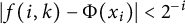 $|f(i, k) - \Phi (x_{i})| < 2^{-i}$
as required. This completes the induction.
$|f(i, k) - \Phi (x_{i})| < 2^{-i}$
as required. This completes the induction.
5.3.3 Finalizing the argument
Let
 $[a_{1}, a_{2}, \ldots ] = x_{\infty } = \lim _{i \to \infty } x_{i}$
. We claim that
$[a_{1}, a_{2}, \ldots ] = x_{\infty } = \lim _{i \to \infty } x_{i}$
. We claim that
 $\Phi (x_{\infty }) < \infty $
and
$\Phi (x_{\infty }) < \infty $
and
 $\Phi (x_{\infty })$
is not computable by any TM.
$\Phi (x_{\infty })$
is not computable by any TM.
We first show that
 $\lim _{n \to \infty }\Phi (x_{i}) < \Phi (x_{0}) + 4 < \infty $
. From (4), we have for all
$\lim _{n \to \infty }\Phi (x_{i}) < \Phi (x_{0}) + 4 < \infty $
. From (4), we have for all
 $i \in \mathbb {N}$
that
$i \in \mathbb {N}$
that
 $$ \begin{align*} \Phi(x_{i}) < \Phi(x_{i-1}) + 2 \cdot 2^{-i+1}, \end{align*} $$
hence,
 $$ \begin{align*} \Phi(x_{i}) < \Phi(x_{0}) + \sum_{j=1}^{i}2^{2} \cdot 2^{-j} \implies \sup_{i \in \mathbb{N}} \Phi(x_{i}) \leq \Phi(x_{0})+4. \end{align*} $$
We now show that
 $\Phi (x_{\infty })$
is finite and equals
$\Phi (x_{\infty })$
is finite and equals
 $\lim _{i\to \infty }\Phi (x_{i})$
. For each i, the sequence
$\lim _{i\to \infty }\Phi (x_{i})$
. For each i, the sequence
 $(f(j,n(i)))_{j=1}^{\infty }$
is Cauchy by (8), hence, it converges to some
$(f(j,n(i)))_{j=1}^{\infty }$
is Cauchy by (8), hence, it converges to some
 $f_{\infty }(n(i))$
. It is clear that
$f_{\infty }(n(i))$
. It is clear that
 $$ \begin{align*} f_{\infty}(n(i)) = \sum_{n=1}^{n(i)} s(i) \cdot \left( \eta_{0}^{\infty} \eta_{1}^{\infty} \dots \eta_{n-1}^{\infty} \right)^{\nu} \cdot u(\eta_{n}^{\infty}) \end{align*} $$
by definition of
 $x_{\infty }$
and by the way, each successive
$x_{\infty }$
and by the way, each successive
 $x_{j}$
was chosen. Since each
$x_{j}$
was chosen. Since each
 $f(j, n(i)) \leq \Phi (x_{j})$
, taking limits on both sides gives
$f(j, n(i)) \leq \Phi (x_{j})$
, taking limits on both sides gives
 $f_{\infty }(n(i)) \leq \Phi (x_{0})+4$
. Thus, the sequence
$f_{\infty }(n(i)) \leq \Phi (x_{0})+4$
. Thus, the sequence
 $(f_{\infty }(n(i)))_{i=1}^{\infty }$
is bounded from above, so the limit superior is finite. But now
$(f_{\infty }(n(i)))_{i=1}^{\infty }$
is bounded from above, so the limit superior is finite. But now
 $$ \begin{align*} \limsup_{i\to\infty}f_{\infty}(n(i)) = \limsup_{i\to\infty} \sum_{n=1}^{n(i)} s(i) \cdot \left( \eta_{0}^{\infty} \eta_{1}^{\infty} \dots \eta_{n-1}^{\infty} \right)^{\nu} \cdot u(\eta_{n}^{\infty}) \geq \Phi(x_{\infty}), \end{align*} $$
showing that
 $\Phi (x_{\infty })$
is finite. Now, we claim that
$\Phi (x_{\infty })$
is finite. Now, we claim that
 $\Phi (x_{\infty }) = \lim _{i\to \infty }\Phi (x_{i})$
. Let
$\Phi (x_{\infty }) = \lim _{i\to \infty }\Phi (x_{i})$
. Let
 $\varepsilon>0$
be given.
$\varepsilon>0$
be given.
-
• Choose
$i_{1}$
large enough so that
$$ \begin{align*} i>i_{1} \implies |f_{\infty}(n(i))-\Phi(x_{\infty})| < \varepsilon/3. \end{align*} $$
-
• Choose
$i_{2}>i_{1}$
large enough so that
$2^{-i_{2}}<\varepsilon /3$
. By (7), we have
$$ \begin{align*} i> i_{2} \implies |f(i, n(i))-\Phi(x_{i})| < \varepsilon/3. \end{align*} $$
-
• Set
$i_{3} = i_{2}+1$
, so that
$2^{-i_{3}+1} < \varepsilon /3$
. Then, for
$i>i_{3}$
, repeated application of (8) yields
$$ \begin{align*} |f(i, n(i))-f_{\infty}(n(i))| \leq \sum_{j=i}^{\infty}|f(j+1, n(i))-f(j, n(i))| < \sum_{j=i}^{\infty}2^{-j} = 2^{-i+1}<\varepsilon/3. \end{align*} $$


Taking
 $i>\max \{i_{1}, i_{2}, i_{3} \}$
, we finally get
$i>\max \{i_{1}, i_{2}, i_{3} \}$
, we finally get
 $$ \begin{align*} & |\Phi(x_{\infty})-\Phi(x_{i})| \\ &\quad \leq |\Phi(x_{\infty})-f_{\infty}(k)|+|f_{\infty}(n(i))-f(i,n(i))|+|f(i,n(i))-\Phi(x_{i})|< \varepsilon. \end{align*} $$
It remains to show that
 $\Phi (x_{\infty })$
is not computable by any of the TMs
$\Phi (x_{\infty })$
is not computable by any of the TMs
 $M^{\phi }_{i}$
, where
$M^{\phi }_{i}$
, where
 $\phi $
is an oracle for
$\phi $
is an oracle for
 $x_{\infty }$
. Let
$x_{\infty }$
. Let
 $\phi _{\infty }$
be the oracle for
$\phi _{\infty }$
be the oracle for
 $x_{\infty }$
which agrees with
$x_{\infty }$
which agrees with
 $\phi _{i}$
on inputs
$\phi _{i}$
on inputs
 $1, 2, \ldots , k_{i+1}$
. This is a valid construction of an oracle by (2) and since
$1, 2, \ldots , k_{i+1}$
. This is a valid construction of an oracle by (2) and since
 $\lim _{i\to \infty }k_{i+1}=\infty $
. To show that
$\lim _{i\to \infty }k_{i+1}=\infty $
. To show that
 $\phi _{\infty }$
is indeed an oracle for
$\phi _{\infty }$
is indeed an oracle for
 $x_{\infty }$
, let
$x_{\infty }$
, let
 $n \in \mathbb {Z}^{+}$
and set i such that
$n \in \mathbb {Z}^{+}$
and set i such that
 $n+1<k_{i}$
. Since
$n+1<k_{i}$
. Since
 $n+1<k_{i}$
implies that
$n+1<k_{i}$
implies that
 $n+j+1<k_{i+j}$
,
$n+j+1<k_{i+j}$
,
 $$ \begin{align*} |\phi_{\infty}(n)-x_{\infty}| & \leq |\phi_{\infty}(n)-x_{i}|+|x_{i}-x_{\infty}| \leq |\phi_{i}(n)-x_{i}| + \sum_{j=i}^{\infty}|x_{j+1}-x_{j}| \\ &< 2^{-(n+1)} + \sum_{j=0}^{\infty}2^{-(k_{i+j}+1)} \leq 2^{-(n+1)} + \sum_{j=0}^{\infty}2^{-(n+j+2)} = 2^{-n}, \end{align*} $$
so
 $\phi _{\infty }$
is indeed an oracle for
$\phi _{\infty }$
is indeed an oracle for
 $x_{\infty }$
. Now, for a contradiction, suppose some TM
$x_{\infty }$
. Now, for a contradiction, suppose some TM
 $M_{j}^{\phi _{\infty }}$
computes
$M_{j}^{\phi _{\infty }}$
computes
 $\Phi (x_{\infty })$
. We have two cases:
$\Phi (x_{\infty })$
. We have two cases:
-
(1)
$j = l_{i}$
for some i. Then,
$M_{l_{i}}^{\phi _{i}}(\hat {a}_{i})$
outputs
$B_{i}$
for which
$B_{i}+2^{-\hat {a}_{i}}<\Phi (x_{i})$
by (5). This same number
$B_{i}$
is output when running
$M_{l_{i}}^{\phi _{\infty }}(\hat {a}_{i})$
. But then so we cannot have
$$ \begin{align*} B_{i}+2^{-\hat{a}_{i}}<\Phi(x_{i})<\Phi(x_{i+1})< \cdots < \Phi(x_{\infty}), \end{align*} $$
$|B_{i}-\Phi (x_{\infty })| \leq 2^{-\hat {a}_{i}}$
, contradicting the assumption that
$M_{l_{i}}^{\phi _{\infty }}$
computes
$\Phi (x_{\infty })$
.
-
(2)
$j \neq l_{i}$
for all i. Choose the smallest
$i>2$
for which
$j<l_{i}$
. Then,
$M_{j}^{\phi _{i-1}}(a_{j})$
outputs
$A_{j}$
for which
$|A_{j}-\Phi (x_{i-1})|>2^{-a_{j}}+\varepsilon _{j}$
, where
$a_{j}$
and
$\varepsilon _{j}$
are from the i-th step of the induction. This same number
$A_{j}$
is output when running
$M_{j}^{\phi _{\infty }}(a_{j})$
. By assumption,
$|A_{j}-\Phi (x_{\infty })|<2^{-a_{j}}$
, hence
$|\Phi (x_{i-1})-\Phi (x_{\infty })|>\varepsilon _{j}$
. But for all
$$ \begin{align*} |\Phi(x_{k})-\Phi(x_{k+1})|<2^{-\hat{a}_{k}+2} \leq 2^{-\hat{n}_{k}+2}<\frac{\varepsilon_{j}}{2^{k}} \end{align*} $$
$k \geq i-1$
, thus a contradiction.
$$ \begin{align*} |\Phi(x_{i-1})-\Phi(x_{\infty})| \leq \sum_{k=i-1}^{\infty}|\Phi(x_{k})-\Phi(x_{k+1})| < \sum_{k=i-1}^{\infty}\frac{\varepsilon_{j}}{2^{k}} \leq \varepsilon_{j}, \end{align*} $$


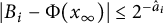


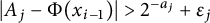


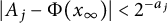
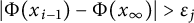


We have shown that none of the TMs
 $M_{j}^{\phi _{\infty }}$
compute
$M_{j}^{\phi _{\infty }}$
compute
 $\Phi (x_{\infty })$
, where
$\Phi (x_{\infty })$
, where
 $\phi _{\infty }$
is an oracle for
$\phi _{\infty }$
is an oracle for
 $x_{\infty }$
. This completes the proof of Theorem 5.2.
$x_{\infty }$
. This completes the proof of Theorem 5.2.
A Proofs of the main technical statements
A.1 Proof of Theorem 3.1
The most involved part of the proof will be showing that conditions (i)–(vii) on G are satisfied by the
 $\alpha $
-continued fraction expansion maps
$\alpha $
-continued fraction expansion maps
 $A_{\alpha }$
for
$A_{\alpha }$
for
 $\alpha \in [1/2, 1]$
.
$\alpha \in [1/2, 1]$
.
Lemma A.1 Conditions (i)–(vii) are satisfied by both the Gauss map and by
 $A_{\alpha }$
for
$A_{\alpha }$
for
 $\alpha \in [1/2, 1)$
.
$\alpha \in [1/2, 1)$
.
Proof Properties (i), (iii), and (v)–(vii) are easy enough that we group them together and prove them at once, and then (ii) and (iv) are verified separately.
(i), (iii), and (v)–(vii). For the Gauss map G,
 $G(J_{i}) = G( (\frac {1}{i+1}, \frac {1}{i}) ) = (0, 1) = (s_{0}, s_{1})$
. It is clear that G is decreasing on
$G(J_{i}) = G( (\frac {1}{i+1}, \frac {1}{i}) ) = (0, 1) = (s_{0}, s_{1})$
. It is clear that G is decreasing on
 $J_{1} = (1/2, 1)$
. Since
$J_{1} = (1/2, 1)$
. Since
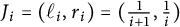 $J_{i} = (\ell _{i}, r_{i}) = (\frac {1}{i+1}, \frac {1}{i})$
, we have
$J_{i} = (\ell _{i}, r_{i}) = (\frac {1}{i+1}, \frac {1}{i})$
, we have
 $$ \begin{align*} \dfrac{r_{i}-\ell_{i}}{\ell_{i}^{2}} < 2 =: D \text{ and } g(i) = \frac{r_{i}}{\ell_{i+1}} \xrightarrow{i \to \infty} 0. \end{align*} $$
Finally, since G is a composition of computable functions, it is computable.
Now, let
 $\alpha \in [1/2, 1)$
, and consider the map
$\alpha \in [1/2, 1)$
, and consider the map
 $A_{\alpha }$
corresponding to
$A_{\alpha }$
corresponding to
 $\alpha $
-continued fraction expansions. Set
$\alpha $
-continued fraction expansions. Set
 $n_{1} := \lceil 1/(1-\alpha ) \rceil $
; this is the smallest integer for which
$n_{1} := \lceil 1/(1-\alpha ) \rceil $
; this is the smallest integer for which
 $1/n_{1} \leq 1-\alpha $
and
$1/n_{1} \leq 1-\alpha $
and
 $A_{\alpha }(1/n_{1}) = 0$
. We restrict the domain and codomain of
$A_{\alpha }(1/n_{1}) = 0$
. We restrict the domain and codomain of
 $A_{\alpha }(x)$
to the maximal invariant set
$A_{\alpha }(x)$
to the maximal invariant set
 $\Lambda \subseteq (s_{0}, s_{1}) := (0, 1/n_{1}) \subseteq (0, 1-\alpha )$
, and henceforth consider
$\Lambda \subseteq (s_{0}, s_{1}) := (0, 1/n_{1}) \subseteq (0, 1-\alpha )$
, and henceforth consider
 $A_{\alpha }: \Lambda \to \Lambda $
. It is clear that
$A_{\alpha }: \Lambda \to \Lambda $
. It is clear that
 $\Lambda $
is a countable disjoint union of connected intervals, which we label
$\Lambda $
is a countable disjoint union of connected intervals, which we label
 $J_{1} = (\ell _{1}, r_{1}), J_{2} = (\ell _{2}, r_{2}), \ldots $
with
$J_{1} = (\ell _{1}, r_{1}), J_{2} = (\ell _{2}, r_{2}), \ldots $
with
 $r_{1}> \ell _{1} \geq r_{2} > \ell _{2} \geq \cdots $
. From maximality of the invariant set and the fact that
$r_{1}> \ell _{1} \geq r_{2} > \ell _{2} \geq \cdots $
. From maximality of the invariant set and the fact that
 $|A_{\alpha }'(x)|>1$
on
$|A_{\alpha }'(x)|>1$
on
 $\Lambda $
, (i) holds. For (vi), computability of
$\Lambda $
, (i) holds. For (vi), computability of
 $A_{\alpha }$
again follows since it is a composition of computable functions. We will make use of the following facts about
$A_{\alpha }$
again follows since it is a composition of computable functions. We will make use of the following facts about
 $A_{\alpha }$
and the intervals
$A_{\alpha }$
and the intervals
 $J_{j}$
:
$J_{j}$
:
-
•
$A_{\alpha }$
is decreasing on
$J_{j}$
for odd j and increasing on
$J_{j}$
for even j. In particular, since
$A_{\alpha }(r_{1}) = A_{\alpha }(1/n_{1}) = 0$
,
$|A_{\alpha }'(x)|>1$
, and
$A_{\alpha }(x)> 0$
,
$A_{\alpha }$
is decreasing on
$J_{1}$
and so (iii) is satisfied. -
• For
$\alpha = 1/2$
, it can be readily computed by solving the equations
$A_{\alpha }(x) = 0$
and
$A_{\alpha }(x) = 1$
that
$n_{1} = 2$
and
$J_{j} = (\ell _{j}, r_{j}) = (\frac {2}{j+4}, \frac {2}{j+3})$
. -
• For
$\alpha \in (1/2, 1)$
, we have
$$ \begin{align*} &\ell_{j}> \frac{2}{2(n_{1}-2+k)+3} \\&= \frac{2}{j+2n_{1}}, r_{j} = \frac{1}{n_{1}-1+k} = \frac{2}{j+2n_{1}-1} \text{ for } j = 2k-1 \text{ odd, and} \\ &\ell_{j} = \frac{1}{n_{1}+k} = \frac{2}{2n_{1}+j}, r_{j} < \frac{2}{2(n_{1}-2+k)+3} = \frac{2}{j+2n_{1}-1} \text{ for } j = 2k \text{ even.} \end{align*} $$


It is easy to verify (v) and (vii) by showing that
 $\dfrac {r_{i}-\ell _{i}}{\ell _{i}^{2}}$
is bounded from above independently of i and that
$\dfrac {r_{i}-\ell _{i}}{\ell _{i}^{2}}$
is bounded from above independently of i and that
 $g(i) \xrightarrow {i \to \infty } 0$
.
$g(i) \xrightarrow {i \to \infty } 0$
.
(ii). For G, we note that
 $G'(x) = 1/x^{2}, G"(x) = 2/x^{3}$
, where it is defined. Since G is decreasing on all
$G'(x) = 1/x^{2}, G"(x) = 2/x^{3}$
, where it is defined. Since G is decreasing on all
 $J_{j}$
, we have
$J_{j}$
, we have
 $\tau _{i,1} = |G'(r_{i})| = i^{2}$
. Taking any
$\tau _{i,1} = |G'(r_{i})| = i^{2}$
. Taking any
 $\sigma>2$
,
$\sigma>2$
,
 $\tau _{i,1}^{-1} < \ell _{i} \sigma $
as needed. Now, set
$\tau _{i,1}^{-1} < \ell _{i} \sigma $
as needed. Now, set
 $\kappa = 2$
. Then, where it is defined, it is easy to check that
$\kappa = 2$
. Then, where it is defined, it is easy to check that
 $(G^{2})"> 0$
and thus
$(G^{2})"> 0$
and thus
 $\tau _{i,2} = |(G^{2})'(\ell _{i})| = (i+1)^{2}$
. Hence, for any
$\tau _{i,2} = |(G^{2})'(\ell _{i})| = (i+1)^{2}$
. Hence, for any
 $1 < \tau < 2$
, we have
$1 < \tau < 2$
, we have
 $\tau _{i,2}^{-1} < \ell _{i} \cdot \tau ^{-1}$
as needed.
$\tau _{i,2}^{-1} < \ell _{i} \cdot \tau ^{-1}$
as needed.
Now, again consider
 $A_{\alpha }$
, for
$A_{\alpha }$
, for
 $\alpha \in [1/2, 1)$
. As for the Gauss map,
$\alpha \in [1/2, 1)$
. As for the Gauss map,
 $A_{\alpha }'(x) = 1/x^{2}, A_{\alpha }"(x) = 2/x^{3}> 0,$
where it is defined. Set
$A_{\alpha }'(x) = 1/x^{2}, A_{\alpha }"(x) = 2/x^{3}> 0,$
where it is defined. Set
 $\kappa = 1$
. Then,
$\kappa = 1$
. Then,
 $\tau _{i,\kappa } = \tau _{i, 1} = 1/r_{i}^{2}$
.
$\tau _{i,\kappa } = \tau _{i, 1} = 1/r_{i}^{2}$
.
-
• Let
$\sigma>1$
be large enough that for all i,
$\sigma> \dfrac {2(2n_{1}+i)}{(i+2n_{1}-1)^{2}}$
. It is easily verified that
$\tau _{i,1}^{-1} < \ell _{i} \sigma $
. -
• Now, note that
$$ \begin{align*} \tau_{i,1}^{-1} = r_{i}^{2} < \ell_{i} \tau^{-1} \iff \dfrac{2(2n_{1}+i)}{(i+2n_{1}-1)^{2}} < \tau^{-1}. \end{align*} $$
Since the left-hand side tends to zero as
$n_{1} \to \infty $
for all
$i \geq 1$
, restricting
$\Lambda $
to a small enough invariant set under
$A_{\alpha }$
, that is, making
$r_{1} = \frac {1}{n_{1}}$
small enough, gives existence of some
$\tau>1$
for which the above holds.


(iv). For the Gauss map, recalling that
 $\varphi = \frac {\sqrt {5}-1}{2} = [1, 1, \ldots ]$
, we have
$\varphi = \frac {\sqrt {5}-1}{2} = [1, 1, \ldots ]$
, we have
 $$ \begin{align*} \delta_{G}(N) = \frac{1}{(N + \varphi)(N + 1 + \varphi)} \text{ and so } \dfrac{r_{N+1}}{\ell_{N+1}} \cdot \dfrac{r_{n} - \ell_{N+1}}{\delta_{G}(N)} < D \end{align*} $$
for some constant D. We first show that (iv) holds for
 $A_{1/2}$
, then for
$A_{1/2}$
, then for
 $A_{\alpha }$
,
$A_{\alpha }$
,
 $\alpha \in (1/2, 1)$
. We denote the symbolic expansion of a point in
$\alpha \in (1/2, 1)$
. We denote the symbolic expansion of a point in
 $\Lambda $
generated by
$\Lambda $
generated by
 $A_{1/2}$
as
$A_{1/2}$
as
 $[a_{1}, a_{2}, a_{3}, \ldots ]_{1/2}$
, and that of a point in the invariant set generated by G as
$[a_{1}, a_{2}, a_{3}, \ldots ]_{1/2}$
, and that of a point in the invariant set generated by G as
 $[a_{1}, a_{2}, a_{3}, \ldots ]_{1}$
. Since the interval
$[a_{1}, a_{2}, a_{3}, \ldots ]_{1}$
. Since the interval
 $J_{1}$
corresponding to
$J_{1}$
corresponding to
 $A_{1/2}$
is contained in the interval
$A_{1/2}$
is contained in the interval
 $J_{2}$
corresponding to G, we have
$J_{2}$
corresponding to G, we have
 $\psi := [1, 1, 1, \ldots ]_{1/2} = [2, 2, 2, \ldots ]_{1} = \sqrt {2}-1$
. For
$\psi := [1, 1, 1, \ldots ]_{1/2} = [2, 2, 2, \ldots ]_{1} = \sqrt {2}-1$
. For
 $N = 2k-1$
odd, the interval
$N = 2k-1$
odd, the interval
 $J_{N}$
corresponding to
$J_{N}$
corresponding to
 $A_{1/2}$
is contained in the interval
$A_{1/2}$
is contained in the interval
 $J_{(N+3)/2}$
corresponding to G, so
$J_{(N+3)/2}$
corresponding to G, so
 $$ \begin{align*} [N, 1, 1, \ldots]_{1/2} = [k+1, 2, 2, \ldots]_{1} = [(N+3)/2, 2, 2, \ldots]_{1} = \dfrac{1}{\frac{N+3}{2}+\psi} = \dfrac{2}{N + 3 + 2\psi}. \end{align*} $$
Now, consider
 $N = 2k$
even. Observe that on
$N = 2k$
even. Observe that on
 $J_{N}, A_{1/2}(x) = 1 - G(x)$
. We have
$J_{N}, A_{1/2}(x) = 1 - G(x)$
. We have
 $$ \begin{align*} [N, 1, 1, \ldots]_{1/2} = (A_{1/2}|_{J_{N}})^{-1}([1, 1, \ldots]_{1/2}) = G_{N/2 + 1}^{-1}(1 - [2, 2, \ldots]_{1}) = \dfrac{2}{N+4-2\psi}. \end{align*} $$
Thus,
 $$ \begin{align*} \delta_{A_{1/2}}(N) &= [N, 1, 1, \ldots]_{1/2} - [N+1, 1, 1, \ldots]_{1/2} \\& = \dfrac{4 - 8\psi}{(N+3+2\psi)(N+5-2\psi)} \text{ if } N \text{ is odd, and} \\ \delta_{A_{1/2}}(N) &= \dfrac{8\psi}{(N+4-2\psi)(N+4+2\psi)} \text{ if } N \text{ is even.} \end{align*} $$
Noting that
 $r_{N} - \ell _{N+1} = \frac {4}{(N+3)(N+5)}$
and
$r_{N} - \ell _{N+1} = \frac {4}{(N+3)(N+5)}$
and
 $\frac {r_{N+1}}{\ell _{N+1}} = \frac {N+5}{N+4}$
, it is clear that some constant D upper-bounds
$\frac {r_{N+1}}{\ell _{N+1}} = \frac {N+5}{N+4}$
, it is clear that some constant D upper-bounds
 $\frac {r_{N+1}}{\ell _{N+1}} \cdot \frac {r_{N}-\ell _{N+1}}{\delta _{A_{1/2}}(N)}$
. Finally, for
$\frac {r_{N+1}}{\ell _{N+1}} \cdot \frac {r_{N}-\ell _{N+1}}{\delta _{A_{1/2}}(N)}$
. Finally, for
 $\alpha \in (1/2, 1)$
, we have
$\alpha \in (1/2, 1)$
, we have
 $A_{1/2} = A_{\alpha }$
on the invariant set
$A_{1/2} = A_{\alpha }$
on the invariant set
 $\Lambda $
corresponding to
$\Lambda $
corresponding to
 $A_{\alpha }$
. Thus, the asymptotic behavior of
$A_{\alpha }$
. Thus, the asymptotic behavior of
 $\ell _{N}$
,
$\ell _{N}$
,
 $r_{N}$
, and
$r_{N}$
, and
 $\delta _{A_{\alpha }}(N)$
is identical, so (iv) holds in this case as well.
$\delta _{A_{\alpha }}(N)$
is identical, so (iv) holds in this case as well.
We can now prove Theorem 3.1 without too much difficulty.
Proof of Theorem 3.1. By Lemma A.1 and since the function u in the definition of
 ${{\mathcal B}}_{\alpha ,u,\nu }$
satisfies
${{\mathcal B}}_{\alpha ,u,\nu }$
satisfies
 $\lim _{x \to 0^{+}}u(x) = \infty $
by assumption, conditions (i)–(vii) on G and (i)–(v) on u hold for
$\lim _{x \to 0^{+}}u(x) = \infty $
by assumption, conditions (i)–(vii) on G and (i)–(v) on u hold for
 ${{\mathcal B}}_{\alpha , u, v}$
. To prove this theorem, it remains to show that for
${{\mathcal B}}_{\alpha , u, v}$
. To prove this theorem, it remains to show that for
 $G = A_{\alpha }$
,
$G = A_{\alpha }$
,
 $\alpha \in [1/2,1]$
, conditions (i)–(v) hold for both
$\alpha \in [1/2,1]$
, conditions (i)–(v) hold for both
 $u(x) = \log ^{n}(1/x), n \in \mathbb {Z}^{+}$
and
$u(x) = \log ^{n}(1/x), n \in \mathbb {Z}^{+}$
and
 $u(x) = x^{-1}$
. It is clear that both these functions are computable on
$u(x) = x^{-1}$
. It is clear that both these functions are computable on
 $\mathbb {R}^{+}$
and tend to infinity near zero. If
$\mathbb {R}^{+}$
and tend to infinity near zero. If
 $\alpha \in [1/2, 1),$
then
$\alpha \in [1/2, 1),$
then
 $s_{1}<1$
, so (ii) in this case is satisfied. Thus, we only need to show (ii) in the case that G is the ordinary Gauss map, and (iii).
$s_{1}<1$
, so (ii) in this case is satisfied. Thus, we only need to show (ii) in the case that G is the ordinary Gauss map, and (iii).
For
 $u(x) = x^{-1}$
, (iii) is obvious. If
$u(x) = x^{-1}$
, (iii) is obvious. If
 $u(x) = \log ^{n}(1/x)$
, then
$u(x) = \log ^{n}(1/x)$
, then
 $|u'(x)| = \frac {n}{x} \cdot \log ^{n-1}(1/x)$
. Since there is some
$|u'(x)| = \frac {n}{x} \cdot \log ^{n-1}(1/x)$
. Since there is some
 $C_{n}>0$
for which
$C_{n}>0$
for which
 $\log ^{n-1}(y) < C_{n}y$
for all large enough y, we have
$\log ^{n-1}(y) < C_{n}y$
for all large enough y, we have
 $\log ^{n-1}(1/x) < \frac {C_{n}}{x}$
for all small enough x. Thus,
$\log ^{n-1}(1/x) < \frac {C_{n}}{x}$
for all small enough x. Thus,
 $|u'(x)| < \frac {nC_{n}}{x^{2}}$
for all small enough x and since
$|u'(x)| < \frac {nC_{n}}{x^{2}}$
for all small enough x and since
 $|u'(x)|$
is bounded for x which is bounded away from zero, there is some
$|u'(x)|$
is bounded for x which is bounded away from zero, there is some
 $C>0$
for which
$C>0$
for which
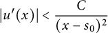 $|u'(x)| < \dfrac {C}{(x-s_{0})^{2}}$
for all
$|u'(x)| < \dfrac {C}{(x-s_{0})^{2}}$
for all
 $x \in (s_{0}, s_{1})$
as needed.
$x \in (s_{0}, s_{1})$
as needed.
Now, suppose G is the Gauss map. Then,
 $u \circ G_{1}^{-1} \circ G_{N}^{-1}(z)$
is decreasing with respect to N since
$u \circ G_{1}^{-1} \circ G_{N}^{-1}(z)$
is decreasing with respect to N since
 $u(\cdot )$
is decreasing, so
$u(\cdot )$
is decreasing, so
 $$ \begin{align*} \frac{u \circ G_{1}^{-1} \circ G_{N}^{-1}(z)}{u \circ G_{1}^{-1} \circ G_{N}^{-1}(w)} \geq \frac{u \circ G_{1}^{-1} \circ G_{N}^{-1}(1)}{u \circ G_{1}^{-1} \circ G_{N}^{-1}(0)} =: v(N). \end{align*} $$
A tedious computation shows that
 $v'(N)>0$
and
$v'(N)>0$
and
 $v(N)>0$
for all N and both
$v(N)>0$
for all N and both
 $u(x) = \log ^{n}(1/x)$
and
$u(x) = \log ^{n}(1/x)$
and
 $u(x) = x^{-1}$
, therefore (ii) holds.
$u(x) = x^{-1}$
, therefore (ii) holds.
A.2 Proofs of the main lemmas
Here, we will prove the three main lemmas used in the above work. Lemma 4.1 will be proven under the weaker assumptions on G and u along with the
 $s(i)$
term in Section 5, and Lemmas 4.2 and 4.3 will be proven under the full assumptions in Section 3. We recall these lemmas below.
$s(i)$
term in Section 5, and Lemmas 4.2 and 4.3 will be proven under the full assumptions in Section 3. We recall these lemmas below.
Lemma 4.1 For any initial segment
 $I = [a_{1}, a_{2}, \ldots , a_{n}]$
, write
$I = [a_{1}, a_{2}, \ldots , a_{n}]$
, write
 $\omega = [a_{1}, a_{2}, \ldots , a_{n}, 1, 1, 1, \ldots ]$
. Then, for any
$\omega = [a_{1}, a_{2}, \ldots , a_{n}, 1, 1, 1, \ldots ]$
. Then, for any
 $\varepsilon>0$
, there is an
$\varepsilon>0$
, there is an
 $m>0$
and an integer N such that if we write
$m>0$
and an integer N such that if we write
 $\beta = [a_{1}, a_{2}, \ldots , a_{n}, 1, 1, \ldots , 1, N, 1, 1, \ldots ]$
, where the N is located in the
$\beta = [a_{1}, a_{2}, \ldots , a_{n}, 1, 1, \ldots , 1, N, 1, 1, \ldots ]$
, where the N is located in the
 $(n+m)$
-th position, then
$(n+m)$
-th position, then
 $$ \begin{align*} \Phi(\omega) + \varepsilon < \Phi(\beta) < \Phi(\omega) + 2\varepsilon. \end{align*} $$
Lemma 4.2 Write
 $\omega = [a_{1}, a_{2}, \ldots , a_{n}, 1, 1, 1, \ldots ]$
. Then, for any
$\omega = [a_{1}, a_{2}, \ldots , a_{n}, 1, 1, 1, \ldots ]$
. Then, for any
 $\varepsilon>0,$
there is an
$\varepsilon>0,$
there is an
 $m_{0}>0$
, which can be computed from
$m_{0}>0$
, which can be computed from
 $(a_{1}, a_{2}, \ldots , a_{n})$
and
$(a_{1}, a_{2}, \ldots , a_{n})$
and
 $\varepsilon $
, such that for any
$\varepsilon $
, such that for any
 $m \geq m_{0}$
and for any tail
$m \geq m_{0}$
and for any tail
 $I = [a_{n+m}, a_{n+m+1}, \ldots ]$
,
$I = [a_{n+m}, a_{n+m+1}, \ldots ]$
,
 $$ \begin{align*} \Phi(\beta^{I})> \Phi(\omega) - \varepsilon, \end{align*} $$
where
 $$ \begin{align*} \beta^{I} = [a_{1}, a_{2}, \ldots, a_{n}, 1, 1, \ldots, 1, a_{n+m}, a_{n+m+1}, \ldots]. \end{align*} $$
Lemma 4.3 Let
 $\omega = [a_{1}, a_{2}, \ldots ]$
be such that
$\omega = [a_{1}, a_{2}, \ldots ]$
be such that
 $\Phi (\omega ) < \infty $
. Write
$\Phi (\omega ) < \infty $
. Write
 $\omega _{k} = [a_{1}, a_{2}, \ldots , a_{k}, 1, 1, \ldots ]$
. Then, for every
$\omega _{k} = [a_{1}, a_{2}, \ldots , a_{k}, 1, 1, \ldots ]$
. Then, for every
 $\varepsilon>0,$
there is an m such that, for all
$\varepsilon>0,$
there is an m such that, for all
 $k \geq m$
,
$k \geq m$
,
 $$ \begin{align*} \Phi(\omega_{k}) < \Phi(\omega) + \varepsilon. \end{align*} $$
Write
 $$ \begin{align*} \beta^{N} = [a_{1}, a_{2}, \ldots, a_{n}, 1, 1, \ldots, 1, N, 1, 1, \ldots], \end{align*} $$
where N is in the
 $(m+n)$
-th position. The following preliminary lemmas are required for all of the main proofs below.
$(m+n)$
-th position. The following preliminary lemmas are required for all of the main proofs below.
Lemma A.2 For any
 $s_{0}<a<s_{1}$
, the function u is bounded on the interval
$s_{0}<a<s_{1}$
, the function u is bounded on the interval
 $[a, s_{1})$
.
$[a, s_{1})$
.
Proof By assumption on u, there is some
 $C>0$
for which
$C>0$
for which
 $-u'(x) < \frac {C}{(x-s_{0})^{2}}$
for all
$-u'(x) < \frac {C}{(x-s_{0})^{2}}$
for all
 $x \in [a, s_{1})$
. Integrating both sides gives
$x \in [a, s_{1})$
. Integrating both sides gives
 $u(x) < \frac {\tilde {C}}{x-s_{0}} \leq \frac {\tilde {C}}{a-s_{0}}$
for another constant
$u(x) < \frac {\tilde {C}}{x-s_{0}} \leq \frac {\tilde {C}}{a-s_{0}}$
for another constant
 $\tilde {C}>0$
and all
$\tilde {C}>0$
and all
 $x \in [a, s_{1})$
.
$x \in [a, s_{1})$
.
Lemma A.3 Let
 $\beta ^{N}, \beta ^{1}$
be as before, let
$\beta ^{N}, \beta ^{1}$
be as before, let
 $\beta ^{I}, \omega $
be as in Lemma 4.2, and let
$\beta ^{I}, \omega $
be as in Lemma 4.2, and let
 $\gamma _{1}, \gamma _{2}$
be two numbers whose symbolic representations coincide in the first
$\gamma _{1}, \gamma _{2}$
be two numbers whose symbolic representations coincide in the first
 $n+m-1$
terms
$n+m-1$
terms
 $[a_{1}, a_{2}, \ldots , a_{n+m-1}]$
(in particular, we could have
$[a_{1}, a_{2}, \ldots , a_{n+m-1}]$
(in particular, we could have
 $\gamma _{1} = \beta ^{N}$
and
$\gamma _{1} = \beta ^{N}$
and
 $\gamma _{2} = \beta ^{1}$
). Then, for g and
$\gamma _{2} = \beta ^{1}$
). Then, for g and
 $m_{g}$
as in (vii), for
$m_{g}$
as in (vii), for
 $\kappa $
as in (ii), and for any N, the following holds:
$\kappa $
as in (ii), and for any N, the following holds:
-
(1) For
$i \leq n+m$
,
$$ \begin{align*} \left | \log \frac{\eta_{i}(\beta^{N})}{\eta_{i}(\beta^{N+1})} \right | < \dfrac{g(N)}{\ell_{1}} \cdot \tau^{1+\frac{i-(n+m)}{\kappa}}. \end{align*} $$
-
(2) For
$i < n+m$
,
$$ \begin{align*} \left | \log \frac{\eta_{i}(\gamma_{1})}{\eta_{i}(\gamma_{2})} \right | < m_{g} \cdot \sigma \cdot \tau^{1 + \frac{i+1-(n+m)}{\kappa}}. \end{align*} $$
-
(3) For all large enough m, there is some positive function f with
$\lim _{m \to \infty }f(m) = 0$
such that for
$i<n+m-1$
,
$$ \begin{align*} \left | \log \frac{u(\eta_{i}(\beta^{I}))}{u(\eta_{i}(\omega))} \right | < f(m). \end{align*} $$
In particular, we could take
$\beta ^{I} = \beta ^{1}$
and
$\omega = \beta ^{N}$
. Clearly,
$0 < \sup _{m \in \mathbb {N}}f(m) =: M < \infty $
.


Proof of (1)
We will first show that for all
 $i,$
we have
$i,$
we have
 $$\begin{align} |\eta_{i}(\beta^{N}) - \eta_{i}(\beta^{N+1})| < g(N) \cdot \tau^{1+\frac{i-(n+m)}{\kappa}}. \end{align} $$
If
 $i=n+m$
, since
$i=n+m$
, since
 $[N, 1, 1, \ldots ] \in J_{N}$
,
$[N, 1, 1, \ldots ] \in J_{N}$
,
 $[N+1, 1, 1, \ldots ] \in J_{N+1}$
, for all
$[N+1, 1, 1, \ldots ] \in J_{N+1}$
, for all
 $N \in \mathbb {N,}$
we have
$N \in \mathbb {N,}$
we have
 $$ \begin{align*} 1 < \dfrac{\eta_{n+m}(\beta^{N})}{\eta_{n+m}(\beta^{N+1})} = \dfrac{[N, 1, 1, \ldots]}{[N+1, 1, 1, \ldots]} < \dfrac{r_{N}}{\ell_{N+1}} < 1 + g(N) \end{align*} $$
and so
 $$ \begin{align*} |\eta_{n+m}(\beta^{N}) - \eta_{n+m}(\beta^{N+1})| < g(N) < g(N) \cdot \tau^{1+\frac{i-(n+m)}{\kappa}}. \end{align*} $$
Now, let
 $1 \leq j < \kappa $
. We wish to show *1
for
$1 \leq j < \kappa $
. We wish to show *1
for
 $i = n+m-j$
. Note that since
$i = n+m-j$
. Note that since
 $|G_{1}'(x)|> 1$
for all
$|G_{1}'(x)|> 1$
for all
 $x \in S$
by (ii) and
$x \in S$
by (ii) and
 $G_{1}$
is
$G_{1}$
is
 $\mathcal {C}^{1}$
, the Inverse Function Theorem gives
$\mathcal {C}^{1}$
, the Inverse Function Theorem gives
 $|(G_{1}^{-1})'(x)| < 1$
for all
$|(G_{1}^{-1})'(x)| < 1$
for all
 $x \in J_{1}$
. Repeatedly applying the Mean Value Theorem gives
$x \in J_{1}$
. Repeatedly applying the Mean Value Theorem gives
 $$ \begin{align*} |\eta_{n+m-j}(\beta^{N}) - \eta_{n+m-j}(\beta^{N+1})| &< |\eta_{n+m}(\beta^{N}) - \eta_{n+m}(\beta^{N+1})| \\ &< g(N) < g(N) \cdot \tau^{1-j / \kappa}. \end{align*} $$
For
 $i = n+m - \kappa $
, since
$i = n+m - \kappa $
, since
 $|(G_{1}^{\kappa })'|>\tau $
by assumption (ii) on G, we similarly use Inverse Function Theorem and Mean Value Theorem (applied to the function
$|(G_{1}^{\kappa })'|>\tau $
by assumption (ii) on G, we similarly use Inverse Function Theorem and Mean Value Theorem (applied to the function
 $G_{1}^{-\kappa }$
this time) to get
$G_{1}^{-\kappa }$
this time) to get
 $$ \begin{align*} |\eta_{n+m-\kappa}(\beta^{N}) - \eta_{n+m-\kappa}(\beta^{N+1})| &< \tau^{-1} \cdot |\eta_{n+m}(\beta^{N}) - \eta_{n+m}(\beta^{N+1})| \\ &< g(N) \cdot \tau^{1+\frac{i-(n+m)}{\kappa}}. \end{align*} $$
To show *1
for all other
 $i>n+m-j$
with
$i>n+m-j$
with
 $j>\kappa $
, we apply the inequality
$j>\kappa $
, we apply the inequality
 $$ \begin{align*} |\eta_{n+m-j}(\beta^{N}) - \eta_{n+m-j}(\beta^{N+1})| < \tau^{-1} \cdot |\eta_{n+m-j+\kappa}(\beta^{N}) - \eta_{n+m-j+\kappa}(\beta^{N+1})| \end{align*} $$
repeatedly until one of the cases
 $i \geq n+m-\kappa $
above is reached.
$i \geq n+m-\kappa $
above is reached.
We now proceed to prove (1). If
 $i=n+m,$
then as before for all
$i=n+m,$
then as before for all
 $N \in \mathbb {Z}^{+}$
, we have
$N \in \mathbb {Z}^{+}$
, we have
 $$ \begin{align*} 1 < \dfrac{\eta_{i}(\beta^{N})}{\eta_{i}(\beta^{N+1})} < 1 + g(N) \end{align*} $$
and so
 $$ \begin{align*} \left| \log \dfrac{\eta_{i}(\beta^{N})}{\eta_{i}(\beta^{N+1})} \right| < \log \left( 1 + g(N) \right) < \log(e^{g(N)}) = g(N) < \dfrac{g(N)}{\ell_{1}} \cdot \tau^{1+\frac{i-(n+m)}{\kappa}}, \end{align*} $$
where we used the inequality
 $1 + \xi < e^{\xi }$
for any
$1 + \xi < e^{\xi }$
for any
 $\xi>0$
.
$\xi>0$
.
Let
 $1 \leq i < n+m$
, and assume
$1 \leq i < n+m$
, and assume
 $\eta _{i}(\beta ^{N})> \eta _{i}(\beta ^{N+1})$
; the complementary case is almost identical. We have
$\eta _{i}(\beta ^{N})> \eta _{i}(\beta ^{N+1})$
; the complementary case is almost identical. We have
 $\eta _{i}(\beta ^{N}), \eta _{i}(\beta ^{N+1})> \ell _{1}$
since they are in
$\eta _{i}(\beta ^{N}), \eta _{i}(\beta ^{N+1})> \ell _{1}$
since they are in
 $J_{1}$
and so from *1
,
$J_{1}$
and so from *1
,
 $$ \begin{align*} &\left| \dfrac{\eta_{i}(\beta^{N}) - \eta_{i}(\beta^{N+1})}{\eta_{i}(\beta^{N+1})} \right| \\ &\quad < \dfrac{g(N)}{\ell_{1}} \cdot \tau^{1+\frac{i-(n+m)} {\kappa}} \text{ and so }1 < \dfrac{\eta_{i}(\beta^{N})}{\eta_{i}(\beta^{N+1})} < 1 + \dfrac{g(N)}{\ell_{1}} \cdot \tau^{1+\frac{i-(n+m)}{\kappa}} \end{align*} $$
As above, this gives the desired inequality.
Proof of (2)
Note that
 $\eta _{i}(\gamma _{1})$
and
$\eta _{i}(\gamma _{1})$
and
 $\eta _{i}(\gamma _{2})$
agree on the first digit of the symbolic expansion for each
$\eta _{i}(\gamma _{2})$
agree on the first digit of the symbolic expansion for each
 $1 \leq i < n+m$
; we write this digit as
$1 \leq i < n+m$
; we write this digit as
 $N_{i}$
.
$N_{i}$
.
We will first show that for all
 $i,$
we have
$i,$
we have
 $$\begin{align} \dfrac{\eta_{i}(\gamma_{1})}{\eta_{i}(\gamma_{2})} < 1 + m_{g} \cdot \sigma \cdot \tau^{1 + \frac{i+1-(n+m)}{\kappa}}. \end{align} $$
If
 $\eta _{i}(\gamma _{1}) < \eta _{i}(\gamma _{2}),$
this is obviously true as the second term on the right-hand side is greater than zero, but to unify the argument, we will not split into cases.
$\eta _{i}(\gamma _{1}) < \eta _{i}(\gamma _{2}),$
this is obviously true as the second term on the right-hand side is greater than zero, but to unify the argument, we will not split into cases.
For
 $i = n+m-1$
, using assumption (vii) on
$i = n+m-1$
, using assumption (vii) on
 $G,$
we compute
$G,$
we compute
 $$ \begin{align*} \dfrac{\eta_{n+m-1}(\gamma_{1})}{\eta_{n+m-1}(\gamma_{2})} < \dfrac{r_{N_{n+m-1}}}{\ell_{N_{n+m-1}}} < 1 + g(N_{n+m-1}) \leq 1 + m_{g} < 1 + m_{g} \cdot \sigma \cdot \tau^{1+\frac{i+1-(n+m)}{\kappa}}. \end{align*} $$
For future use, note that the above inequalities yield
 $$ \begin{align*} \eta_{n+m-1}(\gamma_{1}) - \eta_{n+m-1}(\gamma_{2}) \leq \eta_{n+m-1}(\gamma_{2}) \cdot m_{g} < m_{g}. \end{align*} $$
Now, let
 $1 \leq j < \kappa $
. We want to show *2
for
$1 \leq j < \kappa $
. We want to show *2
for
 $i = n+m-1-j$
. Similar to the proof of (1), we note that
$i = n+m-1-j$
. Similar to the proof of (1), we note that
 $|(G_{N_{n+m-1-j}}^{-1})'(x)| < \tau _{N_{n+m-1-j},1}^{-1}$
for all
$|(G_{N_{n+m-1-j}}^{-1})'(x)| < \tau _{N_{n+m-1-j},1}^{-1}$
for all
 $x \in J_{N_{n+m-1-j}}$
and (ii) gives
$x \in J_{N_{n+m-1-j}}$
and (ii) gives
 $|(G_{N_{t}}^{-1})'(x)| < 1$
for all
$|(G_{N_{t}}^{-1})'(x)| < 1$
for all
 $x \in J_{N_{t}}$
, t arbitrary, so repeatedly applying the Mean Value Theorem,
$x \in J_{N_{t}}$
, t arbitrary, so repeatedly applying the Mean Value Theorem,
 $$ \begin{align*} &\hspace{18px} \eta_{n+m-1-j}(\gamma_{1}) - \eta_{n+m-1-j}(\gamma_{2}) \\ &< |G_{N_{n+m-1-j}}^{-1} \circ \cdots \circ G_{N_{n+m-2}}^{-1}(\eta_{n+m-1}(\gamma_{1})) - G_{N_{n+m-1-j}}^{-1} \circ \cdots \circ G_{N_{n+m-2}}^{-1}(\eta_{n+m-1}(\gamma_{2}))| \\ &< \tau_{N_{n+m-1-j},1}^{-1} \cdot |G_{N_{n+m-j}}^{-1} \circ \cdots \circ G_{N_{n+m-2}}^{-1}(\eta_{n+m-1}(\gamma_{1})) \\ &\quad - G_{N_{n+m-j}}^{-1} \circ \cdots \circ G_{N_{n+m-2}}^{-1}(\eta_{n+m-1}(\gamma_{2}))| \\ &< \tau_{N_{n+m-1-j},1}^{-1} \cdot |\eta_{n+m-1}(\gamma_{1}) - \eta_{n+m-1}(\gamma_{2})| < \tau_{N_{n+m-1-j},1}^{-1} \cdot m_{g} \\ &< \ell_{N_{n+m-1-j}} \cdot \sigma \cdot m_{g} < \eta_{n+m-1-j}(\gamma_{2}) \cdot \sigma \cdot m_{g} \cdot \tau^{1+\frac{i+1-(n+m)}{\kappa}}. \end{align*} $$
Rearranging gives *2
. To show *2
holds for
 $i - l \cdot \kappa $
with
$i - l \cdot \kappa $
with
 $n+m-1-\kappa < i \leq n+m-1$
and
$n+m-1-\kappa < i \leq n+m-1$
and
 $l \in \mathbb {Z}^{+}$
, repeatedly apply the inequality
$l \in \mathbb {Z}^{+}$
, repeatedly apply the inequality
 $$ \begin{align*} &\hspace{18px} \eta_{i-j \cdot \kappa}(\gamma_{1}) - \eta_{i-l \cdot \kappa}(\gamma_{2}) \\ &< |G_{N_{i-l \cdot \kappa}}^{-1} \circ \cdots \circ G_{N_{i-l \cdot \kappa + \kappa - 1}}^{-1}(\eta_{i-(l-1) \cdot \kappa}(\gamma_{1})) - G_{N_{i-l \cdot \kappa}}^{-1} \circ \cdots \\ &\quad \circ G_{N_{i-l \cdot \kappa + \kappa - 1}}^{-1}(\eta_{i-(l-1) \cdot \kappa}(\gamma_{2}))| \\ &= \left| \dfrac{1}{(G^{\kappa})'(\xi)} \right| \cdot |\eta_{i-(l-1) \cdot \kappa}(\gamma_{1}) - \eta_{i-(l-1) \cdot \kappa}(\gamma_{2})| \\ &< \tau^{-1} \cdot |\eta_{i-(l-1) \cdot \kappa}(\gamma_{1}) - \eta_{i-(l-1) \cdot \kappa}(\gamma_{2})| \end{align*} $$
(where
 $\xi \in J_{N_{i-j \cdot \kappa }}$
is from the Mean Value Theorem and we made use of (ii)) until one of the base cases above is reached.
$\xi \in J_{N_{i-j \cdot \kappa }}$
is from the Mean Value Theorem and we made use of (ii)) until one of the base cases above is reached.
We now suppose without loss of generality that
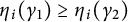 $\eta _{i}(\gamma _{1}) \geq \eta _{i}(\gamma _{2})$
. Using the inequality
$\eta _{i}(\gamma _{1}) \geq \eta _{i}(\gamma _{2})$
. Using the inequality
 $1 + \xi < e^{\xi }$
for any
$1 + \xi < e^{\xi }$
for any
 $\xi>0$
with *2
gives
$\xi>0$
with *2
gives
 $$ \begin{align*} 0 &< \log \dfrac{\eta_{i}(\gamma_{1})}{\eta_{i}(\gamma_{2})} \\ &< \log \left( 1 + m_{g} \cdot \sigma \cdot \tau^{1 + \frac{i+1-(n+m)}{\kappa}} \right) < \log(e^{m_{g} \cdot \sigma \cdot \tau^{1 + \frac{i+1-(n+m)}{\kappa}}}) = m_{g} \cdot \sigma \cdot \tau^{1 + \frac{i+1-(n+m)}{\kappa}}. \end{align*} $$
On the other hand, the inequalities
 $\dfrac {1}{1-\xi }> e^{\xi }$
and
$\dfrac {1}{1-\xi }> e^{\xi }$
and
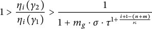 $1> \dfrac {\eta _{i}(\gamma _{2})}{\eta _{i}(\gamma _{1})} > \dfrac {1}{1+m_{g} \cdot \sigma \cdot \tau ^{1 + \frac {i+1-(n+m)}{\kappa }}}$
give
$1> \dfrac {\eta _{i}(\gamma _{2})}{\eta _{i}(\gamma _{1})} > \dfrac {1}{1+m_{g} \cdot \sigma \cdot \tau ^{1 + \frac {i+1-(n+m)}{\kappa }}}$
give
 $$ \begin{align*} 0> \log \dfrac{\eta_{i}(\gamma_{2})}{\eta_{i}(\gamma_{1})} & > \log \left( \dfrac{1}{1+m_{g} \cdot \sigma \cdot \tau^{1 + \frac{i+1-(n+m)}{\kappa}}} \right) \\ & > \log(e^{-m_{g} \cdot \sigma \cdot \tau^{1 + \frac{i+1-(n+m)}{\kappa}}}) = -m_{g} \cdot \sigma \cdot \tau^{1 + \frac{i+1-(n+m)}{\kappa}}. \end{align*} $$
Combining these together yields
 $$ \begin{align*} \left| \log \dfrac{\eta_{i}(\gamma_{1})}{\eta_{i}(\gamma_{2})} \right| < m_{g} \cdot \sigma \cdot \tau^{1 + \frac{i+1-(n+m)}{\kappa}}. \end{align*} $$
Proof of (3)
Let
 $(\delta (m))_{m=1}^{\infty }$
be a sequence of positive numbers such that
$(\delta (m))_{m=1}^{\infty }$
be a sequence of positive numbers such that
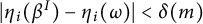 $|\eta _{i}(\beta ^{I})-\eta _{i}(\omega )| < \delta (m)$
for all
$|\eta _{i}(\beta ^{I})-\eta _{i}(\omega )| < \delta (m)$
for all
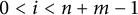 $0 < i < n+m-1$
and
$0 < i < n+m-1$
and
 $N \in \mathbb {N}$
, and
$N \in \mathbb {N}$
, and
 $\lim _{m \to \infty } \delta (m) = 0$
. We claim that
$\lim _{m \to \infty } \delta (m) = 0$
. We claim that
 $\eta _{i}(\beta ^{I})$
is uniformly bounded away from
$\eta _{i}(\beta ^{I})$
is uniformly bounded away from
 $0$
and
$0$
and
 $1$
for all I and
$1$
for all I and
 $0<i<n+m-1$
. Note that
$0<i<n+m-1$
. Note that
 $$ \begin{align*} &\eta_{i}(\beta^{I}) = [1, 1, \ldots]\qquad\quad \text{for } n<i<n+m-1, \\ &\eta_{i}(\beta^{I}) = [a_{n}, 1, \ldots]\qquad\, \text{ for } i=n, \text{ and} \\ &\eta_{i}(\beta^{I}) = [a_{i}, a_{i+1}, \ldots]\quad \text{ for } 0<i<n. \end{align*} $$
Call these first two digits
 $p_{i}$
and
$p_{i}$
and
 $q_{i}$
, noting that
$q_{i}$
, noting that
 $p_{i} = q_{i} = p_{n+1} = q_{n+1}$
if
$p_{i} = q_{i} = p_{n+1} = q_{n+1}$
if
 $n<i<n+m-1$
. Let
$n<i<n+m-1$
. Let
 $$ \begin{align*} &\eta_{\min} = \min_{0 < i < n+m-1} [p_{i}, q_{i}, \ldots] = \min_{0 < i \leq n+1} [p_{i}, q_{i}, \ldots] = \min_{0 < i \leq n+1} (G_{p_{i}}^{-1} \circ G_{q_{i}}^{-1})((s_{0}, s_{1})), \\ &\eta_{\max} = \max_{0 < i < n+m-1} [p_{i}, q_{i}, \ldots] = \max_{0 < i \leq n+1} [p_{i}, q_{i}, \ldots] = \max_{0 < i \leq n+1} (G_{p_{i}}^{-1} \circ G_{q_{i}}^{-1})((s_{0}, s_{1})). \end{align*} $$
It is clear that if
 $p_{i} \neq 1$
or
$p_{i} \neq 1$
or
 $q_{i} \neq 1,$
then
$q_{i} \neq 1,$
then
 $s_{0} < \eta _{\min } < \eta _{\max } < s_{1}$
. If
$s_{0} < \eta _{\min } < \eta _{\max } < s_{1}$
. If
 $p_{i}=q_{i}=1$
, by assumption (iii) on
$p_{i}=q_{i}=1$
, by assumption (iii) on
 $G,$
we have
$G,$
we have
 $$ \begin{align*} (G_{p_{i}}^{-1} \circ G_{q_{i}}^{-1})((s_{0}, s_{1})) = G_{p_{i}}^{-1}(G_{q_{i}}^{-1}(s_{1}), s_{1}) = (G_{q_{i}}^{-1}(s_{1}), (G_{p_{i}}^{-1} \circ G_{q_{i}}^{-1})(s_{1})) \end{align*} $$
with
 $s_{0} < G_{q_{i}}^{-1}(s_{1}) < (G_{p_{i}}^{-1} \circ G_{q_{i}}^{-1})(s_{1}) < s_{1}$
. Hence,
$s_{0} < G_{q_{i}}^{-1}(s_{1}) < (G_{p_{i}}^{-1} \circ G_{q_{i}}^{-1})(s_{1}) < s_{1}$
. Hence,
 $s_{0} < \eta _{\min } < \eta _{\max } < s_{1}$
in all cases. Thus,
$s_{0} < \eta _{\min } < \eta _{\max } < s_{1}$
in all cases. Thus,
 $$ \begin{align*} \eta_{i}(\beta^{I}) \in [\eta_{\min}, \eta_{\max}] \subseteq (s_{0}, s_{1}). \end{align*} $$
Clearly,
 $\eta _{i}(\omega ) \in [\eta _{\min }, \eta _{max}]$
as well. Now, letting
$\eta _{i}(\omega ) \in [\eta _{\min }, \eta _{max}]$
as well. Now, letting
 $$ \begin{align*} \tilde{u} = \inf_{x \in [\eta_{\min}, \eta_{\max}]}u(x), \end{align*} $$
we have
 $\tilde {u}>0$
since u is continuous and positive on the compact subset
$\tilde {u}>0$
since u is continuous and positive on the compact subset
 $[\eta _{\min }, \eta _{\max }]$
.
$[\eta _{\min }, \eta _{\max }]$
.
Since u is continuous, it is uniformly continuous on
 $[\eta _{\min }, \eta _{\max }]$
, hence admits a continuous and strictly increasing modulus of continuity
$[\eta _{\min }, \eta _{\max }]$
, hence admits a continuous and strictly increasing modulus of continuity
 $\sigma : [0, \infty ) \to [0, \infty )$
such that
$\sigma : [0, \infty ) \to [0, \infty )$
such that
 $\lim _{t \to 0} \sigma (t) = \sigma (0) = 0$
and for all
$\lim _{t \to 0} \sigma (t) = \sigma (0) = 0$
and for all
 $x_{1}, x_{2} \in [\eta _{\min }, \eta _{\max }], |u(x_{1})-u(x_{2})| \leq \sigma (|x_{1}-x_{2}|)$
.
$x_{1}, x_{2} \in [\eta _{\min }, \eta _{\max }], |u(x_{1})-u(x_{2})| \leq \sigma (|x_{1}-x_{2}|)$
.
Now, fix m large enough that
 $1 - \dfrac {\sigma (\delta (m))}{\tilde {u}}> 0$
, and let
$1 - \dfrac {\sigma (\delta (m))}{\tilde {u}}> 0$
, and let
 $0 < i < n+m-1$
and
$0 < i < n+m-1$
and
 $N \in \mathbb {N}$
. Then,
$N \in \mathbb {N}$
. Then,
 $$ \begin{align*} &|u(\eta_{i}(\beta^{I}))-u(\eta_{i}(\omega))| \leq \sigma(|\eta_{i}(\beta^{I})-\eta_{i}(\gamma_{2})|) < \sigma(\delta(m)) \\[0.4em] &\implies \left| \dfrac{u(\eta_{i}(\beta^{I}))}{u(\eta_{i}(\omega))} -1 \right| < \dfrac{\sigma(\delta(m))}{u(\eta_{i}(\omega))} \leq \dfrac{\sigma(\delta(m))}{\tilde{u}} \\[0.4em] &\implies \left| \log \left( \dfrac{u(\eta_{i}(\beta^{I}))}{u(\eta_{i}(\omega))} \right) \right| < \max \left\{ \left| \log \left( 1-\dfrac{\sigma(\delta(m))}{\tilde{u}} \right) \right|, \left| \log \left( 1+\dfrac{\sigma(\delta(m))}{\tilde{u}} \right) \right| \right\}\\ & =: f(m), \end{align*} $$
with
 $$ \begin{align*} \lim_{m \to \infty}f(m) = 0 \text{ since } \lim_{\delta(m) \to 0^{+}} \log \left( 1 \pm \dfrac{\sigma(\delta(m))}{\tilde{u}} \right) = 0 \end{align*} $$
and
 $f(m)>0$
since
$f(m)>0$
since
 $\dfrac {\sigma (\delta (m))}{\tilde {u}}> 0$
for all m.
$\dfrac {\sigma (\delta (m))}{\tilde {u}}> 0$
for all m.
Lemma A.4 There is some
 $\rho <1$
such that for any
$\rho <1$
such that for any
 $k>1$
and
$k>1$
and
 $x \in \Lambda $
,
$x \in \Lambda $
,
 $\eta _{k-1}(x) \cdot \eta _{k}(x) < \rho $
.
$\eta _{k-1}(x) \cdot \eta _{k}(x) < \rho $
.
Proof If
 $s_{1}<1,$
we can take
$s_{1}<1,$
we can take
 $\rho = s_{1}$
, so suppose
$\rho = s_{1}$
, so suppose
 $s_{1} = 1$
. By the decreasing assumption (iii) on
$s_{1} = 1$
. By the decreasing assumption (iii) on
 $G_{1}$
, it is easily checked that there are some
$G_{1}$
, it is easily checked that there are some
 $a_{*}, b_{*} \in (s_{0}, s_{1})$
for which
$a_{*}, b_{*} \in (s_{0}, s_{1})$
for which
 $G(S \cap [a_{*}, 1)) \subseteq (s_{0}, b_{*})$
.
$G(S \cap [a_{*}, 1)) \subseteq (s_{0}, b_{*})$
.
-
• If
$G^{k-1}(x)<a_{*}$
, then since
$G^{k}(x) < 1,$
we have
$G^{k}(x) \cdot G^{k-1}(x) < a_{*} < 1$
. -
• If
$a_{*} \leq G^{k-1}(x) < 1$
, then
$G^{k}(x) = G(G^{k-1}(x)) < b_{*}$
and so
$G^{k}(x) \cdot G^{k-1}(x) < b_{*} < 1$
.

Taking
 $\rho = \max \{a_{*}, b_{*}\}$
completes the proof.
$\rho = \max \{a_{*}, b_{*}\}$
completes the proof.
A.3 Proof of Lemmas 4.2 and 4.3
Lemma A.5 There is a constant D such that for any
 $\gamma _{1}, \gamma _{2} \in \Lambda $
with
$\gamma _{1}, \gamma _{2} \in \Lambda $
with
 $\gamma _{1} = [a, \ldots ]$
,
$\gamma _{1} = [a, \ldots ]$
,
 $\gamma _{2} = [a, \ldots ]$
for some
$\gamma _{2} = [a, \ldots ]$
for some
 $a \in \mathbb {Z}^{+}$
, we have
$a \in \mathbb {Z}^{+}$
, we have
 $$ \begin{align*} \left| u\left( \gamma_{1} \right) - u\left( \gamma_{2} \right) \right| < D. \end{align*} $$
Proof If
 $\gamma _{1} = \gamma _{2}$
, we are done; suppose
$\gamma _{1} = \gamma _{2}$
, we are done; suppose
 $\gamma _{1} < \gamma _{2}$
. Define
$\gamma _{1} < \gamma _{2}$
. Define
 $x(a) := \gamma _{1}$
and
$x(a) := \gamma _{1}$
and
 $h(a) = \gamma _{2} - \gamma _{1}> 0$
. By Taylor’s theorem,
$h(a) = \gamma _{2} - \gamma _{1}> 0$
. By Taylor’s theorem,
 $$ \begin{align*} \left| u(\gamma_{1}) - u(\gamma_{2}) \right| = h(a) \cdot \left| u'(x(a)) + R_{1}(x(a)) \right| \leq \dfrac{h(a)}{(x(a)-s_{0})^{2}} + h(a) \cdot |R_{1}(x(a))|, \end{align*} $$
where we used assumption (iii) on u and where
 $R_{1}$
is the first-order Taylor remainder. But now
$R_{1}$
is the first-order Taylor remainder. But now
 $$ \begin{align*} \dfrac{h(a)}{(x(a)-s_{0})^{2}} = \dfrac{\gamma_{2}-\gamma_{1}}{(\gamma_{1}-s_{0})^{2}} < \dfrac{r_{a}-\ell_{a}}{(\ell_{a}-s_{0})^{2}} < C_{1} \end{align*} $$
for some constant
 $C_{1}$
independent of a, where we used assumption (v) on G. Since
$C_{1}$
independent of a, where we used assumption (v) on G. Since
 $$ \begin{align*} h(a) \cdot |R(x(a))| \to 0 \text{ as } a \to \infty, \end{align*} $$
 $h(a) \cdot |R(x(a))| < C_{2}$
for some constant
$h(a) \cdot |R(x(a))| < C_{2}$
for some constant
 $C_{2}$
. Taking
$C_{2}$
. Taking
 $D = C_{1} + C_{2}$
completes the proof.
$D = C_{1} + C_{2}$
completes the proof.
We are now ready to prove Lemmas 4.2 and 4.3.
Proof of Lemma 4.2
We will first show that such an
 $m_{0}$
exists, and then give an algorithm to compute it.
$m_{0}$
exists, and then give an algorithm to compute it.
Note that the sum in the expression for
 $\Phi (\omega )$
converges, because its tail converges:
$\Phi (\omega )$
converges, because its tail converges:
 $$ \begin{align*} & \sum_{i=n+1}^{\infty} \left( \eta_{0}(\omega) \dots \eta_{i-1}(\omega) \right)^{\nu} \cdot u(\eta_{i}(\omega)) \\ &\quad \leq u(\eta_{n+1}(\omega)) \cdot (\eta_{n}(\omega))^{\nu} \cdot \sum_{i=n+1}^{\infty} (\eta_{n+1}(\omega))^{\nu} < \infty \end{align*} $$
since
 $(\eta _{n+1}(\omega ))^{\nu } < s_{1} \leq 1$
for
$(\eta _{n+1}(\omega ))^{\nu } < s_{1} \leq 1$
for
 $\nu> 0$
. Hence, there is an
$\nu> 0$
. Hence, there is an
 $m_{1}>1$
such that the tail of the sum
$m_{1}>1$
such that the tail of the sum
 $$ \begin{align*} \sum_{i \geq n+m_{1}} \left( \eta_{1}(\omega) \dots \eta_{i-1}(\omega) \right)^{\nu} \cdot u(\eta_{i}(\omega)) < \dfrac{\varepsilon}{2}. \end{align*} $$
If needed, additionally make
 $m_{1}$
large enough that Lemma A.3 (3) applies for all
$m_{1}$
large enough that Lemma A.3 (3) applies for all
 $m \geq m_{1}$
. We will show how to choose
$m \geq m_{1}$
. We will show how to choose
 $m_{0}>m_{1}$
to satisfy the conclusion of the lemma.
$m_{0}>m_{1}$
to satisfy the conclusion of the lemma.
By Lemma A.3 (2) and (3), for any
 $\beta ^{I}$
and any
$\beta ^{I}$
and any
 $i \leq n+m_{1}$
, we have
$i \leq n+m_{1}$
, we have
 $$ \begin{align*} &\hspace{12px} \left| \log \dfrac{ \left( \eta_{0}(\beta^{I}) \dots \eta_{i-1}(\beta^{I}) \right)^{\nu} \cdot u(\eta_{i}(\beta^{I})) }{ \left( \eta_{0}(\omega) \dots \eta_{i-1}(\omega) \right)^{\nu} \cdot u(\eta_{i}(\omega)) } \right| \\ &= \left| \nu \cdot \log \frac{ \eta_{0}(\beta^{I}) \dots \eta_{i-1}(\beta^{I}) }{ \eta_{0}(\omega) \dots \eta_{i-1}(\omega) } + \log \frac{ u(\eta_{i}(\beta^{I})) }{ u(\eta_{i}(\omega)) } \right| \\ &< \nu \cdot \left( \sum_{j=1}^{i-1} m_{g} \cdot \sigma \cdot \tau^{1 + \frac{j+1-(n+m)}{\kappa}} \right) + f(m) < \nu \sigma \cdot m_{g} \cdot \tau^{1 + \frac{2-(n+m)}{\kappa}} \left( \dfrac{\tau^{i}-1}{\tau^{1/\kappa}-1} \right) + f(m) \\ &< \nu \sigma \cdot m_{g} \cdot \tau^{1 + \frac{2-(n+m)}{\kappa}} \left( \dfrac{\tau^{n+m_{1}}}{\tau^{1/\kappa}-1} \right) + f(m) \leq \nu \sigma \cdot m_{g} \cdot \dfrac{\tau^{1+m_{1}+\frac{2-m}{\kappa}}}{\tau^{1/\kappa}-1} + f(m). \end{align*} $$
We can choose
 $m_{0}$
sufficiently large so that
$m_{0}$
sufficiently large so that
 $\exp (\nu \sigma \cdot m_{g} \cdot \dfrac {\tau ^{1+m_{1}+\frac {2-m}{\kappa }}}{\tau ^{1/\kappa }-1} + f(m) )> 1 - \dfrac {\varepsilon }{2 \cdot \Phi (\omega )}$
for
$\exp (\nu \sigma \cdot m_{g} \cdot \dfrac {\tau ^{1+m_{1}+\frac {2-m}{\kappa }}}{\tau ^{1/\kappa }-1} + f(m) )> 1 - \dfrac {\varepsilon }{2 \cdot \Phi (\omega )}$
for
 $m \geq m_{0}$
and also
$m \geq m_{0}$
and also
 $$ \begin{align*} & \left( \eta_{1}(\beta^{I}) \dots \eta_{i-1}(\beta^{I}) \right)^{\nu} \cdot u(\eta_{i}(\beta^{I})) \\ &\quad > \left( 1 - \dfrac{\varepsilon}{2 \cdot \Phi(\omega)} \right) \cdot \left( \eta_{1}(\omega) \dots \eta_{i-1}(\omega) \right)^{\nu} \cdot u(\eta_{i}(\omega)) \end{align*} $$
for
 $i \leq n+m_{1}$
. Now, for any
$i \leq n+m_{1}$
. Now, for any
 $\beta ^{I}$
, we have
$\beta ^{I}$
, we have
 $$ \begin{align*} \Phi(\beta^{I}) &\geq \sum_{i=1}^{n+m_{1}-1} \left( \eta_{1}(\beta^{I}) \dots \eta_{i-1}(\beta^{I}) \right)^{\nu} \cdot u(\eta_{i}(\beta^{I})) \\ &> \sum_{i=1}^{n+m_{1}-1} \left( 1 - \dfrac{\varepsilon}{2 \cdot \Phi(\omega)} \right) \cdot \left( \eta_{1}(\omega) \dots \eta_{i-1}(\omega) \right)^{\nu} \cdot u(\eta_{i}(\omega)) \\ &> \left( 1 - \dfrac{\varepsilon}{2 \cdot \Phi(\omega)} \right) \left( \Phi(\omega) - \dfrac{\varepsilon}{2} \right) > \Phi(\omega) - \varepsilon. \end{align*} $$
Since the symbolic representation of
 $\omega $
ends with all ones, for any specific
$\omega $
ends with all ones, for any specific
 $(a_{1}, a_{2}, \ldots , a_{n}),$
we can compute
$(a_{1}, a_{2}, \ldots , a_{n}),$
we can compute
 $\Phi (\omega )$
by Proposition 4.4. This allows us to compute
$\Phi (\omega )$
by Proposition 4.4. This allows us to compute
 $m_{1}$
by iteratively checking whether
$m_{1}$
by iteratively checking whether
 $$ \begin{align*} \sum_{i \geq n+m_{1}} \left( \eta_{0}(\omega) \dots \eta_{i-1}(\omega) \right)^{\nu} \cdot u(\eta_{i}(\omega)) < \dfrac{\varepsilon}{2} \end{align*} $$
for each
 $m_{1}>1$
. Then, for each candidate
$m_{1}>1$
. Then, for each candidate
 $m_{0}> m_{1}$
, since we can compute
$m_{0}> m_{1}$
, since we can compute
 $\Phi (\omega )$
and
$\Phi (\omega )$
and
 $\left ( \eta _{0}(\omega ) \dots \eta _{i-1}(\omega ) \right )^{\nu } \cdot u(\eta _{i}(\omega ))$
and left-compute
$\left ( \eta _{0}(\omega ) \dots \eta _{i-1}(\omega ) \right )^{\nu } \cdot u(\eta _{i}(\omega ))$
and left-compute
 $\left ( \eta _{0}(\beta ^{I}) \dots \eta _{i-1}(\beta ^{I}) \right )^{\nu } \cdot u(\eta _{i}(\beta ^{I}))$
for each individual i by assumption (v) on u and computability assumption (vi) on G, we can iteratively check whether the following two conditions hold:
$\left ( \eta _{0}(\beta ^{I}) \dots \eta _{i-1}(\beta ^{I}) \right )^{\nu } \cdot u(\eta _{i}(\beta ^{I}))$
for each individual i by assumption (v) on u and computability assumption (vi) on G, we can iteratively check whether the following two conditions hold:
-
(1)
$\exp \left (\nu \sigma \cdot m_{g} \cdot \dfrac {\tau ^{1+m_{1}+\frac {2-m}{\kappa }}}{\tau ^{1/\kappa }-1} + f(m) \right )> 1 - \dfrac {\varepsilon }{2 \cdot \Phi (\omega )}$
. -
(2) For every
$i \leq n+m_{1}$
,
$$ \begin{align*} &\left( \eta_{0}(\beta^{I}) \dots \eta_{i-1}(\beta^{I}) \right)^{\nu} \cdot u(\eta_{i}(\beta^{I})) \\ & \quad > \left( 1 - \dfrac{\varepsilon}{2 \cdot \Phi(\omega)} \right) \cdot \left( \eta_{0}(\omega) \dots \eta_{i-1}(\omega) \right)^{\nu} \cdot u(\eta_{i}(\omega)). \end{align*} $$


We only need to be able to left-compute
 $\left ( \eta _{0}(\beta ^{I}) \dots \eta _{i-1}(\beta ^{I}) \right )^{\nu } \cdot u(\eta _{i}(\beta ^{I}))$
because of the strict inequality in condition (2). Since we have shown that there must exist
$\left ( \eta _{0}(\beta ^{I}) \dots \eta _{i-1}(\beta ^{I}) \right )^{\nu } \cdot u(\eta _{i}(\beta ^{I}))$
because of the strict inequality in condition (2). Since we have shown that there must exist
 $m_{1}>m_{0}$
for which these hold, this algorithm terminates and we eventually find the
$m_{1}>m_{0}$
for which these hold, this algorithm terminates and we eventually find the
 $m_{1}$
we are looking for.
$m_{1}$
we are looking for.
Proof of Lemma 4.3
Let
 $i \leq k-1$
for some integer
$i \leq k-1$
for some integer
 $k>1$
. We will first show that
$k>1$
. We will first show that
 $$ \begin{align*} \rho_{1} < \dfrac{u(\eta_{i}(\omega_{k}))}{u(\eta_{i}(\omega))} < \rho_{2} \end{align*} $$
for some
 $0 < \rho _{1} < \rho _{2} < \infty $
, independent of i and k. Since
$0 < \rho _{1} < \rho _{2} < \infty $
, independent of i and k. Since
 $i \leq k-1$
, the symbolic representations of
$i \leq k-1$
, the symbolic representations of
 $\eta _{i}(\omega _{k}), \eta _{i}(\omega )$
coincide in the first two terms, call them a and b. So, we can write
$\eta _{i}(\omega _{k}), \eta _{i}(\omega )$
coincide in the first two terms, call them a and b. So, we can write
 $$ \begin{align*} &x := \eta_{i}(\omega_{k}) = [a, b, T_{1}], \\ &y := \eta_{i}(\omega) = [a, b, T_{2}], \end{align*} $$
where
 $T_{1}, T_{2}$
are the infinite tails of the symbolic expansions of
$T_{1}, T_{2}$
are the infinite tails of the symbolic expansions of
 $ \eta _{i}(\omega _{k}), \eta _{i}(\omega )$
respectively. Since u is
$ \eta _{i}(\omega _{k}), \eta _{i}(\omega )$
respectively. Since u is
 $\mathcal {C}^{1}$
, we have
$\mathcal {C}^{1}$
, we have
 $$ \begin{align*} u(y) = u(x) + \int_{x}^{y} u'(t) \,dt \end{align*} $$
and so by assumption (iii) on u and (v) on G,
 $$ \begin{align*} \left| \dfrac{u(y)}{u(x)} - 1 \right| &= \dfrac{1}{u(x)} \left| \int_{x}^{y} u'(t) \,dt \right| \leq \dfrac{1}{u(x)} \left| \int_{x}^{y} \dfrac{C}{(t-s_{0})^{2}} \,dt \right| \\ &= \dfrac{C}{u(x)} \left| \dfrac{1}{x-s_{0}} - \dfrac{1}{y-s_{0}} \right| \\[0.8em] &< \dfrac{C}{u(x)} \left( \dfrac{1}{\ell_{i}-s_{0}} - \dfrac{1}{r_{i}-s_{0}} \right) < \dfrac{C}{u(x)} \cdot \dfrac{r_{i} - \ell_{i}}{(\ell_{i}-s_{0})^{2}} < \dfrac{\tilde{C}}{u(x)}. \end{align*} $$
for some constant
 $\tilde {C}>0$
. By assumption (i) on u, there is some
$\tilde {C}>0$
. By assumption (i) on u, there is some
 $l_{1} \in (0, 1)$
such that
$l_{1} \in (0, 1)$
such that
 $\dfrac {1}{u(\xi )} < \dfrac {1}{2\tilde {C}}$
for
$\dfrac {1}{u(\xi )} < \dfrac {1}{2\tilde {C}}$
for
 $\xi \in (0, l_{1})$
. Thus, if a is large enough such that
$\xi \in (0, l_{1})$
. Thus, if a is large enough such that
 $x, y \in (0, l_{1})$
, say
$x, y \in (0, l_{1})$
, say
 $a \geq N_{1} \in \mathbb {Z}^{+}$
, then
$a \geq N_{1} \in \mathbb {Z}^{+}$
, then
 $$ \begin{align*} \left| \dfrac{u(x)}{u(y)} - 1 \right| < \dfrac{\tilde{C}}{2\tilde{C}} = \dfrac{1}{2}. \end{align*} $$
If
 $1 < a < N_{1}$
, then
$1 < a < N_{1}$
, then
 $x, y \in [l_{1}', l_{2}']$
for some
$x, y \in [l_{1}', l_{2}']$
for some
 $0<l_{1}'<l_{2}'<1$
, thus
$0<l_{1}'<l_{2}'<1$
, thus
 $u(x), u(y)$
are bounded away from
$u(x), u(y)$
are bounded away from
 $0$
and
$0$
and
 $\infty $
, so
$\infty $
, so
 $\rho _{1}' < \frac {u(x)}{u(y)} < \rho _{2}'$
for some
$\rho _{1}' < \frac {u(x)}{u(y)} < \rho _{2}'$
for some
 $0 < \rho _{1}' < \rho _{2}' < \infty $
.
$0 < \rho _{1}' < \rho _{2}' < \infty $
.
Now, suppose
 $a=1$
. If
$a=1$
. If
 $s_{1}<1$
, then
$s_{1}<1$
, then
 $x, y \in J_{1}$
with
$x, y \in J_{1}$
with
 $J_{1}$
bounded away from
$J_{1}$
bounded away from
 $0$
and
$0$
and
 $1$
, thus u is bounded away from
$1$
, thus u is bounded away from
 $0$
and infinity on
$0$
and infinity on
 $J_{1}$
. Now, suppose
$J_{1}$
. Now, suppose
 $s_{1}=1$
. It follows immediately from assumption (ii) on u that for large enough b, say
$s_{1}=1$
. It follows immediately from assumption (ii) on u that for large enough b, say
 $b \geq N_{2}$
,
$b \geq N_{2}$
,
 $\frac {u(x)}{u(y)}$
is bounded away from
$\frac {u(x)}{u(y)}$
is bounded away from
 $0$
and infinity. Therefore,
$0$
and infinity. Therefore,
 $\rho _{1}" < \frac {u(x)}{u(y)} < \rho _{2}"$
for some
$\rho _{1}" < \frac {u(x)}{u(y)} < \rho _{2}"$
for some
 $0<\rho _{1}"<\rho _{2}"<\infty $
.
$0<\rho _{1}"<\rho _{2}"<\infty $
.
Putting all this together, letting
 $\rho _{1} = \min \{ \frac {1}{2}, \rho _{1}', \rho _{1}" \}>0$
and
$\rho _{1} = \min \{ \frac {1}{2}, \rho _{1}', \rho _{1}" \}>0$
and
 $\rho _{2} = \max \{ \frac {1}{2}, \rho _{2}', \rho _{2}" \} < \infty ,$
we have for any
$\rho _{2} = \max \{ \frac {1}{2}, \rho _{2}', \rho _{2}" \} < \infty ,$
we have for any
 $\omega _{k}$
and
$\omega _{k}$
and
 $\omega $
that
$\omega $
that
 $\rho _{1} < \frac {u(\omega _{k})}{u(\omega )} < \rho _{2}$
and so
$\rho _{1} < \frac {u(\omega _{k})}{u(\omega )} < \rho _{2}$
and so
 $\left | \log \frac {u(\omega _{k})}{u(\omega )} \right | < D_{1} < \infty $
for some constant
$\left | \log \frac {u(\omega _{k})}{u(\omega )} \right | < D_{1} < \infty $
for some constant
 $D_{1}>0$
.
$D_{1}>0$
.
Returning to the proof of the lemma, since the sum in the expression for
 $\Phi (\omega )$
converges, we can split this sum as
$\Phi (\omega )$
converges, we can split this sum as
 $$ \begin{align*} \Phi(\omega) = \underbrace{\sum_{i=1}^{s} \left( \eta_{0}(\omega) \dots \eta_{i-1}(\omega) \right)^{\nu} \cdot u(\eta_{i}(\omega))}_{\text{"head"}} + \underbrace{\sum_{i=s+1}^{\infty} \left( \eta_{0}(\omega) \dots \eta_{i-1}(\omega) \right)^{\nu} \cdot u(\eta_{i}(\omega))}_{\text{"tail"}} \end{align*} $$
so that “tail”
 $ < \dfrac {\varepsilon }{2 \left ( \exp \left ( \nu \sigma \cdot m_{g} \cdot \frac {\tau }{\tau ^{1/\kappa }-1} + D_{1} \right ) \right )}$
. If needed, additionally make s large enough so that
$ < \dfrac {\varepsilon }{2 \left ( \exp \left ( \nu \sigma \cdot m_{g} \cdot \frac {\tau }{\tau ^{1/\kappa }-1} + D_{1} \right ) \right )}$
. If needed, additionally make s large enough so that
 $$ \begin{align*} \dfrac{\rho^{\nu s/2}}{1-\rho^{\nu/2}} < \dfrac{\varepsilon}{4 \left( \exp \left( \nu \sigma \cdot m_{g} \cdot \frac{\tau}{\tau^{1/\kappa}-1} \right) \cdot D_{2} + u(\varphi) \right)}, \end{align*} $$
where
 $\varphi = [1, 1, \ldots ]$
,
$\varphi = [1, 1, \ldots ]$
,
 $\rho $
is as in Lemma A.4, and
$\rho $
is as in Lemma A.4, and
 $D_{2}$
is the constant from Lemma A.5.
$D_{2}$
is the constant from Lemma A.5.
Since
 $\sum _{i=1}^{s} \left ( \eta _{0}(\cdot ) \dots \eta _{i-1}(\cdot ) \right )^{\nu } \cdot u(\eta _{i}(\cdot ))$
is a finite sum of functions continuous on a neighborhood of
$\sum _{i=1}^{s} \left ( \eta _{0}(\cdot ) \dots \eta _{i-1}(\cdot ) \right )^{\nu } \cdot u(\eta _{i}(\cdot ))$
is a finite sum of functions continuous on a neighborhood of
 $\omega $
, it is continuous on some interval containing
$\omega $
, it is continuous on some interval containing
 $\omega $
. Noting that
$\omega $
. Noting that
 $\omega _{k} \to \omega $
, there is some
$\omega _{k} \to \omega $
, there is some
 $m>s$
such that for any
$m>s$
such that for any
 $k \geq m$
,
$k \geq m$
,
 $$ \begin{align*} \sum_{i=1}^{s} \left( \eta_{0}(\omega_{k}) \dots \eta_{i-1}(\omega_{k}) \right)^{\nu} \cdot u(\eta_{i}(\omega_{k})) < \sum_{i=1}^{s} \left( \eta_{0}(\omega) \dots \eta_{i-1}(\omega) \right)^{\nu} \cdot u(\eta_{i}(\omega)) + \varepsilon/4. \end{align*} $$
We now want to bound the change from
 $$ \begin{align*} \left( \eta_{0}(\omega_{k}) \dots \eta_{i-1}(\omega_{k}) \right)^{\nu} \cdot u(\eta_{i}(\omega_{k})) \text{ to } \left( \eta_{0}(\omega) \dots \eta_{i-1}(\omega) \right)^{\nu} \cdot u(\eta_{i}(\omega)) \end{align*} $$
for
 $i>s$
. We consider these terms individually for
$i>s$
. We consider these terms individually for
 $s<i \leq k-1, i=k$
, and
$s<i \leq k-1, i=k$
, and
 $i \geq k+1$
.
$i \geq k+1$
.
-
• For
$s<i \leq k-1$
. Taking
$n+m := k+1$
in Lemma A.3 (2), since
$\omega _{k}$
and
$\omega $
coincide in the first
$k=n+m-1$
terms, we have
$$ \begin{align*} &\left| \log \frac{ \left( \eta_{0}(\omega_{k}) \dots \eta_{i-1}(\omega_{k}) \right)^{\nu} \cdot u(\eta_{i}(\omega_{k})) }{ \left( \eta_{0}(\omega) \dots \eta_{i-1}(\omega) \right)^{\nu} \cdot u(\eta_{i}(\omega) )} \right| \\ &= \left| \nu \cdot \log \frac{\eta_{0}(\omega_{k}) \dots \eta_{i-1}(\omega_{k}) }{\eta_{0}(\omega) \dots \eta_{i-1}(\omega) } + \log \frac{u(\eta_{i}(\omega_{k}))}{u(\eta_{i}(\omega))} \right| \\ &< \nu \cdot \left( \sum_{j=1}^{i-1} m_{g} \cdot \sigma \cdot \tau^{1 + \frac{j-k}{\kappa}} \right) + D_{1} < \nu \sigma \cdot m_{g} \cdot \dfrac{\tau^{1+\frac{i-k}{\kappa}}}{\tau^{1/\kappa}-1} + D_{1} \leq \nu \sigma \cdot m_{g} \cdot \dfrac{\tau^{1-\frac{1}{\kappa}}}{\tau^{1/\kappa}-1} + D_{1}. \end{align*} $$
Hence, in this case, each term can increase by a factor of at most
$\exp \left (\nu \sigma \cdot m_{g} \cdot \frac {\tau ^{1-\frac {1}{\kappa }}}{\tau ^{1/\kappa }-1} + D_{1} \right )$
. -
• For
$i=k$
. We have where we had previously gotten
$$ \begin{align*} \left| u(\eta_{i}(\omega)) - u(\eta_{i}(\omega_{k})\right)| = \left| u\left( [a_{k}, \ldots] \right) - u\left( [a_{k}, \ldots] \right) \right| < D_{2}, \end{align*} $$
$D_{2}$
from Lemma A.5. Now, by Lemma A.3 (2), so
$$ \begin{align*} \left| \log \frac{ \left( \eta_{0}(\omega_{k}) \dots \eta_{i-1}(\omega_{k}) \right)^{\nu}}{ \left( \eta_{0}(\omega) \dots \eta_{i-1}(\omega) \right)^{\nu}} \right| &= \nu \cdot \left| \log \frac{\eta_{0}(\omega_{k}) \dots \eta_{i-1}(\omega_{k})}{\eta_{0}(\omega) \dots \eta_{i-1}(\omega)} \right| \\ &< \nu \cdot \left( \sum_{j=1}^{i-1} m_{g} \cdot \sigma \cdot \tau^{1 + \frac{j-k}{\kappa}} \right) \\ &< \nu \sigma \cdot m_{g} \cdot \dfrac{\tau^{1+\frac{i-k}{\kappa}}}{\tau^{1/\kappa}-1} = \nu \sigma \cdot m_{g} \cdot \dfrac{\tau}{\tau^{1/\kappa}-1}, \end{align*} $$
$\left ( \eta _{0}(\omega _{k}) \dots \eta _{i-1}(\omega _{k}) \right )^{\nu } < \exp \left ( \nu \sigma \cdot m_{g} \cdot \frac {\tau }{\tau ^{1/\kappa }-1} \right ) \cdot \left ( \eta _{0}(\omega ) \dots \eta _{i-1}(\omega ) \right )^{\nu }$
. Combining these estimates and using the value
$\rho <1$
from Lemma A.4, we get
$$ \begin{align*} &\left( \eta_{0}(\omega_{k}) \dots \eta_{i-1}(\omega_{k}) \right)^{\nu} \cdot u(\eta_{i}(\omega_{k})) \\ &\quad \leq \exp \left( \nu \sigma \cdot m_{g} \cdot \frac{\tau}{\tau^{1/\kappa}-1} \right) \cdot \left( \eta_{0}(\omega) \dots \eta_{i-1}(\omega) \right)^{\nu} \cdot \left( u(\eta_{i}(\omega)) + D_{2} \right) \\ &\quad < \exp \left( \nu \sigma \cdot m_{g} \cdot \frac{\tau}{\tau^{1/\kappa}-1} \right) \cdot \left( \eta_{0}(\omega) \dots \eta_{i-1}(\omega) \right)^{\nu} \cdot u(\eta_{i}(\omega)) \\ &\qquad + \exp \left( \nu \sigma \cdot m_{g} \cdot \frac{\tau}{\tau^{1/\kappa}-1} \right) \cdot D_{2} \cdot \rho^{\nu (i-1)/2}. \end{align*} $$
-
• For
$i \geq k+1$
. Noting that
$u(\eta _{i}(\omega _{k})) = u(\eta _{i}(\omega _{k}))$
, by Lemma A.4, we have
$$ \begin{align*} \left( \eta_{0}(\omega_{k}) \dots \eta_{i-1}(\omega_{k}) \right)^{\nu} \cdot u(\eta_{i}(\omega_{k})) < \rho^{\nu (i-1)/2} \cdot u(\varphi). \end{align*} $$


Therefore, for any
 $i>s$
,
$i>s$
,
 $$ \begin{align*} &\left( \eta_{0}(\omega_{k}) \dots \eta_{i-1}(\omega_{k}) \right)^{\nu} \cdot u(\eta_{i}(\omega_{k})) \\ &\quad < \exp \left( \nu \sigma \cdot m_{g} \cdot \frac{\tau}{\tau^{1/\kappa}-1} + D_{1} \right) \cdot \left( \eta_{0}(\omega) \dots \eta_{i-1}(\omega) \right)^{\nu} \cdot u(\eta_{i}(\omega)) \\ & \qquad + \left( \exp \left( \nu \sigma \cdot m_{g} \cdot \frac{\tau}{\tau^{1/\kappa}-1} \right) \cdot D_{2} + u(\varphi) \right) \cdot \rho^{\nu (i-1)/2}. \end{align*} $$
Finally, noting that
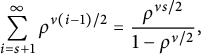 $$ \begin{align*} \sum_{i=s+1}^{\infty} \rho^{\nu (i-1)/2} = \dfrac{\rho^{\nu s/2}}{1-\rho^{\nu/2}}, \end{align*} $$
for such a
 $k,$
we have
$k,$
we have
 $$ \begin{align*} &\Phi(\omega_{k}) = \text{"head"}(\omega_{k}) + \text{"tail"}(\omega_{k}) \\ &\quad < \left( \text{"head"}(\omega) + \dfrac{\varepsilon}{4} \right) + \left( \exp \left( \nu \sigma \cdot m_{g} \cdot \frac{\tau}{\tau^{1/\kappa}-1} + D_{1} \right) \cdot \text{"tail"}(\omega) \right.\ \\ & \qquad + \left.\ \left( \exp \left( \nu \sigma \cdot m_{g} \cdot \frac{\tau}{\tau^{1/\kappa}-1} \right) \cdot D_{2} + u(\varphi) \right) \cdot \dfrac{\rho^{\nu s/2}}{1-\rho^{\nu/2}} \right) \\ &\quad < \text{"head"}(\omega) + \dfrac{\varepsilon}{4} + \exp \left( \nu \sigma \cdot m_{g} \cdot \frac{\tau}{\tau^{1/\kappa}-1} + D_{1} \right) \cdot \dfrac{\varepsilon}{2 \left( \exp \left( \nu \sigma \cdot m_{g} \cdot \frac{\tau}{\tau^{1/\kappa}-1} + D_{1} \right) \right)} \\ & \qquad + \left( \exp \left( \nu \sigma \cdot m_{g} \cdot \frac{\tau}{\tau^{1/\kappa}-1} \right) \cdot D_{2} + u(\varphi) \right) \cdot \dfrac{\varepsilon}{4 \left( \exp \left( \nu \sigma \cdot m_{g} \cdot \frac{\tau}{\tau^{1/\kappa}-1} \right) \cdot D_{2} + u(\varphi) \right)} \\ &\quad = \text{"head"}(\omega) + \dfrac{\varepsilon}{4} + \dfrac{\varepsilon}{2} + \dfrac{\varepsilon}{4} < \Phi(\omega) + \varepsilon. \end{align*} $$
A.4 Proof of Lemma 4.1
Write
 $$ \begin{align*} \Phi^{-}(\omega) = \Phi(\omega) - s(n+m) \cdot \left( \eta_{1}(\omega) \eta_{2}(\omega) \dots \eta_{n+m-1}(\omega) \right)^{\nu} \cdot u(\eta_{n+m}(\omega)). \end{align*} $$
The value of the integer
 $m>0$
is yet to be determined.
$m>0$
is yet to be determined.
Lemma A.6 For any
 $\omega $
of the form as in Lemma 4.1 and for any
$\omega $
of the form as in Lemma 4.1 and for any
 $\varepsilon>0$
, there is an
$\varepsilon>0$
, there is an
 $m_{0}>0$
such that, for any N and any
$m_{0}>0$
such that, for any N and any
 $m \geq m_{0}$
,
$m \geq m_{0}$
,
 $$ \begin{align*} | \Phi^{-}(\beta^{N}) - \Phi^{-}(\beta^{1}) | < \frac{\varepsilon}{4}. \end{align*} $$
Proof Noting that
 $\eta _{n+m-1}(\beta ^{N}) \in (\ell _{1}, s_{1})$
for all
$\eta _{n+m-1}(\beta ^{N}) \in (\ell _{1}, s_{1})$
for all
 $N \in \mathbb {Z}^{+}$
, by Lemma A.2, we have some
$N \in \mathbb {Z}^{+}$
, by Lemma A.2, we have some
 $C>0$
such that
$C>0$
such that
 $0 \leq u(\eta _{n+m-1}(\beta ^{N})) < C$
for all N. Now, the sum in the expression for
$0 \leq u(\eta _{n+m-1}(\beta ^{N})) < C$
for all N. Now, the sum in the expression for
 $\Phi (\beta ^{1})$
converges because its tail converges absolutely:
$\Phi (\beta ^{1})$
converges because its tail converges absolutely:
 $$ \begin{align*} \sum_{i=n+1}^{\infty} \left| s(i) \cdot \left( \eta_{0}(\beta^{1}) \dots \eta_{i-1}(\beta^{1}) \right)^{\nu} \cdot u(\eta_{i}(\beta^{1})) \right| = u(\beta^{1}) \cdot \sum_{i=n+1}^{\infty} \left( (\beta^{1})^{\nu} \right)^{i} < \infty \end{align*} $$
since
 $(\beta ^{1})^{\nu } < s_{1} \leq 1$
for
$(\beta ^{1})^{\nu } < s_{1} \leq 1$
for
 $\nu> 0$
. Hence, there is an
$\nu> 0$
. Hence, there is an
 $m_{1}>1$
, make it large enough that Lemma A.3 (3) applies for all
$m_{1}>1$
, make it large enough that Lemma A.3 (3) applies for all
 $m \geq m_{1}$
, such that the tail of the sum satisfies
$m \geq m_{1}$
, such that the tail of the sum satisfies
 $$ \begin{align*} \sum_{i\geq n+m_{1}} s(i) \cdot \left( \eta_{0}(\beta^{1}) \dots \eta_{i-1}(\beta^{1}) \right)^{\nu} \cdot u(\eta_{i}(\beta^{1})) < \frac{\varepsilon}{4(1 + D)}, \end{align*} $$
where
 $M>0$
is as in Lemma A.3 (3), and D is defined as
$M>0$
is as in Lemma A.3 (3), and D is defined as
 $$ \begin{align*} D = \exp \left( \nu \left( \frac{m_{g} \sigma \tau^{3}}{\tau^{1/\kappa} -1} + \left| \log \left( \frac{C}{u(\ell_{1})} \right) \right| \right) + M \right). \end{align*} $$
We will now show how to choose
 $m_{0}>m_{1}$
to satisfy the conclusion of the lemma.
$m_{0}>m_{1}$
to satisfy the conclusion of the lemma.
We bound the influence of the change from
 $\beta ^{1}$
to
$\beta ^{1}$
to
 $\beta ^{N}$
using Lemma A.3 (2) and (3). The influence on each of the “head elements” (
$\beta ^{N}$
using Lemma A.3 (2) and (3). The influence on each of the “head elements” (
 $i<n+m_{1}$
) is bounded by
$i<n+m_{1}$
) is bounded by
 $$ \begin{align*} &\left| \log \frac{ s(i) \cdot \left( \eta_{0}(\beta^{1}) \dots \eta_{i-1}(\beta^{1}) \right)^{\nu} \cdot u(\eta_{i}(\beta^{1})) }{ s(i) \cdot \left( \eta_{0}(\beta^{N}) \dots \eta_{i-1}(\beta^{N}) \right)^{\nu} \cdot u(\eta_{i}(\beta^{N})) } \right| \\ &\quad = \left| \nu \cdot \log \frac{ \eta_{0}(\beta^{1}) \dots \eta_{i-1}(\beta^{1}) }{ \eta_{0}(\beta^{N}) \dots \eta_{i-1}(\beta^{N}) } + \log \frac{ u(\eta_{i}(\beta^{1})) }{ u(\eta_{i}(\beta^{N})) } \right| \\ &\quad < \nu \cdot \left( \sum_{j=1}^{i-1} m_{g} \cdot \sigma \cdot \tau^{1 + \frac{j+1-(n+m)}{\kappa}} \right) + f(m) \leq \nu \sigma \cdot m_{g} \cdot \dfrac{\tau^{m_{1} + \frac{2 - m}{\kappa}}}{\tau^{1/\kappa}-1} + f(m). \end{align*} $$
By making m sufficiently large (i.e., by choosing a sufficiently large
 $m_{0}$
), we can ensure that
$m_{0}$
), we can ensure that
 $$ \begin{align*} 1 - \frac{\varepsilon}{4(1 + D) \cdot \Phi(\beta^{1})} & < \frac{ s(i) \cdot \left( \eta_{0}(\beta^{N}) \dots \eta_{i-1}(\beta^{N}) \right)^{\nu} \cdot u(\eta_{i}(\beta^{N})) }{ s(i) \cdot \left( \eta_{0}(\beta^{1}) \dots \eta_{i-1}(\beta^{1}) \right)^{\nu} \cdot u(\eta_{i}(\beta^{1})) } < 1\\ &\quad + \frac{\varepsilon}{4(1 + D) \cdot \Phi(\beta^{1})}. \end{align*} $$
Hence,
 $$ \begin{align*} &\Big| s(i) \cdot \left( \eta_{0}(\beta^{N}) \dots \eta_{i-1}(\beta^{N}) \right)^{\nu} \cdot u(\eta_{i}(\beta^{N})) \\ & \quad - s(i) \cdot \left( \eta_{0}(\beta^{1}) \dots \eta_{i-1}(\beta^{1}) \right)^{\nu} \cdot u(\eta_{i}(\beta^{1})) \Big| \\ & < \frac{\varepsilon}{4(1 + D) \cdot \Phi(\beta^{1})} \cdot \left( \eta_{0}(\beta^{1}) \dots \eta_{i-1}(\beta^{1}) \right)^{\nu} \cdot u(\eta_{i}(\beta^{1})). \end{align*} $$
Adding the inequalities for
 $i=1, 2, \ldots , n+m_{1}-1$
, we obtain
$i=1, 2, \ldots , n+m_{1}-1$
, we obtain
 $$ \begin{align*} & \bigg\rvert \sum_{i=1}^{n+m_{1}-1} s(i) \cdot \left( \eta_{0}(\beta^{N}) \dots \eta_{i-1}(\beta^{N}) \right)^{\nu} \cdot u(\eta_{i}(\beta^{N})) \\ & \quad - \sum_{i=1}^{n+m_{1}-1} s(i) \cdot \left( \eta_{0}(\beta^{1}) \dots \eta_{i-1}(\beta^{1}) \right)^{\nu} \cdot u(\eta_{i}(\beta^{1})) \bigg\rvert \\ & < \frac{\varepsilon}{4(1 + D) \cdot \Phi(\beta^{1})} \sum_{i=1}^{n+m_{1}-1} \left( \eta_{0}(\beta^{1}) \dots \eta_{i-1}(\beta^{1}) \right)^{\nu} \cdot u(\eta_{i}(\beta^{1})) = \frac{\varepsilon}{4(1 + D)}. \end{align*} $$
Thus, the influence on the “head” of
 $\Phi ^{-}$
is bounded by
$\Phi ^{-}$
is bounded by
 $\dfrac {\varepsilon }{4(1 + D)}$
. To bound the influence on the “tail,” we consider three kinds of terms
$\dfrac {\varepsilon }{4(1 + D)}$
. To bound the influence on the “tail,” we consider three kinds of terms
 $s(i) \cdot \left ( \eta _{0}(\beta ^{N}) \dots \eta _{i-1}(\beta ^{N}) \right )^{\nu } \cdot u(\eta _{i}(\beta ^{N}))$
: those for which
$s(i) \cdot \left ( \eta _{0}(\beta ^{N}) \dots \eta _{i-1}(\beta ^{N}) \right )^{\nu } \cdot u(\eta _{i}(\beta ^{N}))$
: those for which
 $n+m_{1} \leq i \leq n+m-2$
,
$n+m_{1} \leq i \leq n+m-2$
,
 $i = m+n-1$
, and
$i = m+n-1$
, and
 $i \geq m+n+1$
(recall that the
$i \geq m+n+1$
(recall that the
 $i=n+m$
term is not in
$i=n+m$
term is not in
 $\Phi ^{-}$
).
$\Phi ^{-}$
).
-
• For
$n+m_{1} \leq i \leq n+m-2$
. By Lemma A.3 (2) and (3), and by the work above,
$$ \begin{align*} &\left| \log \frac{ s(i) \cdot \left( \eta_{0}(\beta^{1}) \dots \eta_{i-1}(\beta^{1}) \right)^{\nu} \cdot u(\eta_{i}(\beta^{1})) }{ s(i) \cdot \left( \eta_{0}(\beta^{N}) \dots \eta_{i-1}(\beta^{N}) \right)^{\nu} \cdot u(\eta_{i}(\beta^{N})) } \right| \\ & < \nu \cdot \left( \sum_{j=1}^{i-1} m_{g} \cdot \sigma \cdot \tau^{1 + \frac{j+1-(n+m)}{\kappa}} \right) + f(m) \\ &\leq \nu \sigma \cdot m_{g} \cdot \tau^{1+\frac{2-(n+m)}{\kappa}} \left( \dfrac{\tau^{i}}{\tau^{1/\kappa}-1} \right) + f(m) \leq \nu \sigma \cdot m_{g} \cdot \dfrac{\tau}{\tau^{1/\kappa}-1} + M. \end{align*} $$
Where
$M>0$
is as in Lemma A.3 (3). Hence, in this case, each term can increase or decrease by a factor of at most
$\exp \left ( \frac {\nu \sigma m_{g} \tau }{\tau ^{1/ \kappa } - 1} + M \right )$
. -
• For
$i=n+m-1$
. Recall that for all
$N \in \mathbb {Z}^{+}$
,
$0 \leq u(\eta _{n+m-1}(\beta ^{N})) < C$
. Thus, we have
$$ \begin{align*} &\log \frac{ s(i) \cdot \left( \eta_{0}(\beta^{N}) \dots \eta_{i-1}(\beta^{N}) \right)^{\nu} \cdot u(\eta_{i}(\beta^{N})) }{ s(i) \cdot \left( \eta_{0}(\beta^{1}) \dots \eta_{i-1}(\beta^{1}) \right)^{\nu} \cdot u(\eta_{i}(\beta^{1})) } \leq \log \frac{ \left( \eta_{0}(\beta^{N}) \dots \eta_{i-1}(\beta^{N}) \right)^{\nu} \cdot C }{ \left( \eta_{0}(\beta^{1}) \dots \eta_{i-1}(\beta^{1}) \right)^{\nu} \cdot u(\ell_{1}) } \\ &< \nu \cdot \left( \sum_{j=1}^{n+m-2} m_{g} \cdot \sigma \cdot \tau^{1 + \frac{j+1-(n+m)}{\kappa}} + \log \left( \dfrac{C}{u(\ell_{1})} \right) \right) < \nu \cdot \left( \dfrac{m_{g} \cdot \sigma \cdot \tau^{2}}{\tau^{1/ \kappa} -1} + \log \left( \dfrac{C}{u(\ell_{1})} \right) \right). \end{align*} $$
Hence, this term could increase or decrease by a factor of at most
$\exp \left ( \nu \cdot \left ( \frac {m_{g} \sigma \tau ^{2}}{\tau ^{1/ \kappa } -1} + \log \left ( \frac {C}{u(\ell _{1})} \right ) \right ) \right )$
. -
• For
$i \geq n+m+1$
. Note that the
$\eta _{j}$
for
$j>n+m$
are not affected by the change, and the change decreases
$\eta _{n+m}$
, so that
$\eta _{n+m}(\beta ^{N}) \leq \eta _{n+m}(\beta ^{1})$
and thus
$\left ( \eta _{n+m}(\beta ^{N}) \right )^{\nu } \leq \left ( \eta _{n+m}(\beta ^{1}) \right )^{\nu }$
. Hence,
$$ \begin{align*} &\log \frac{ s(i) \cdot \left( \eta_{0}(\beta^{N}) \dots \eta_{i-1}(\beta^{N}) \right)^{\nu} u(\eta_{i}(\beta^{N})) }{ s(i) \cdot \left( \eta_{0}(\beta^{1}) \dots \eta_{i-1}(\beta^{1}) \right)^{\nu} u(\eta_{i}(\beta^{1})) } = \log \frac{ \left( \eta_{0}(\beta^{N}) \dots \eta_{n+m}(\beta^{N}) \right)^{\nu} }{ \left( \eta_{0}(\beta^{1}) \dots \eta_{n+m}(\beta^{1}) \right)^{\nu} } \\ &\leq \log \frac{ \left( \eta_{0}(\beta^{N}) \dots \eta_{n+m-1}(\beta^{N}) \right)^{\nu} }{ \left( \eta_{0}(\beta^{1}) \dots \eta_{n+m-1}(\beta^{1}) \right)^{\nu} } < \nu \cdot \sum_{j=1}^{n+m-1} m_{g} \cdot \sigma \cdot \tau^{1 + \frac{j+1-(n+m)}{\kappa}} < \dfrac{\nu \cdot m_{g} \cdot \sigma \cdot \tau^{3}}{\tau^{1/ \kappa} - 1}. \end{align*} $$
So, in this case, each term could increase or decrease by a factor of at most
$\exp \left ( \frac {\nu m_{g} \sigma \tau ^{3}}{\tau ^{1/ \kappa }-1} \right )$
.


We see that after the change, each term of the tail could increase or decrease by a factor of
 $$ \begin{align*} \exp \left( \nu \left( \frac{m_{g} \sigma \tau^{3}}{\tau^{1/\kappa} -1} + \left| \log \left( \frac{C}{u(\ell_{1})} \right) \right| \right) + M \right) =: D \end{align*} $$
at most. So the value of the tail remains in the interval
 $\left [-\dfrac {D \cdot \varepsilon }{4(1 + D)}, \dfrac {D \cdot \varepsilon }{4(1 + D)} \right ]$
, hence the change in the tail is bounded by
$\left [-\dfrac {D \cdot \varepsilon }{4(1 + D)}, \dfrac {D \cdot \varepsilon }{4(1 + D)} \right ]$
, hence the change in the tail is bounded by
 $\dfrac {D \cdot \varepsilon }{4(1 + D)}$
.
$\dfrac {D \cdot \varepsilon }{4(1 + D)}$
.
Therefore, the total change in
 $\Phi ^{-}$
is bounded by
$\Phi ^{-}$
is bounded by
 $$ \begin{align*} \text{change in the "head" } + \text{ change in the "tail"} < \frac{\varepsilon}{4(1 + D)} + \frac{D \cdot \varepsilon}{4(1 + D)} = \frac{\varepsilon}{4}. \end{align*} $$
Lemma A.7 For any
 $\varepsilon $
and for the same
$\varepsilon $
and for the same
 $m_{0}(\varepsilon )$
as in Lemma A.6, for any
$m_{0}(\varepsilon )$
as in Lemma A.6, for any
 $m \geq m_{0}$
and N,
$m \geq m_{0}$
and N,
 $$ \begin{align*} |\Phi^{-}(\beta^{N}) - \Phi(\beta^{N+1})| < \frac{\varepsilon}{2}. \end{align*} $$
Proof We have
 $$ \begin{align*} |\Phi^{-}(\beta^{N}) - \Phi(\beta^{N+1})| \leq |\Phi^{-}(\beta^{N}) - \Phi(\beta^{1})| + |\Phi^{-}(\beta^{N+1}) - \Phi(\beta^{1})| < \frac{\varepsilon}{4} + \frac{\varepsilon}{4} = \frac{\varepsilon}{2}. \end{align*} $$
We will now take a closer look at the term
 $$ \begin{align*} \Phi^{1}(\omega) := s(n+m) \cdot \left( \eta_{1}(\omega) \dots \eta_{n+m-1}(\omega) \right)^{\nu} \cdot u(\eta_{n+m}(\omega)) = \Phi(\omega) - \Phi^{-}(\omega). \end{align*} $$
Lemma A.8 There exists some m, which can be made arbitrarily large, such that for any N,
 $$ \begin{align*} \Phi^{1}(\beta^{N+1}) - \Phi^{1}(\beta^{N}) < \frac{\varepsilon}{2}. \end{align*} $$
Proof We assume throughout that
 $s(n+m) = 1$
. By assumption on
$s(n+m) = 1$
. By assumption on
 $s(\cdot )$
, there are infinitely many m such that this holds, so we can take m arbitrarily large within the course of the proof.
$s(\cdot )$
, there are infinitely many m such that this holds, so we can take m arbitrarily large within the course of the proof.
According to Lemma A.3 (1),
 $$ \begin{align*} &\left| \log \frac{ s(n+m) \cdot \left( \eta_{0}(\beta^{N+1}) \dots \eta_{n+m-1}(\beta^{N+1})) \right)^{\nu} }{ s(n+m) \cdot \left( \eta_{0}(\beta^{N}) \dots \eta_{n+m-1}(\beta^{N})) \right)^{\nu} } \right| < \nu \cdot \sum_{i=1}^{n+m-1} \dfrac{g(N)}{\ell_{1}} \cdot \tau^{1 + \frac{i-(n+m)}{\kappa}} \\ &= \nu \cdot g(N) \cdot \tau^{1 + \frac{1-(n+m)}{\kappa}} \cdot \dfrac{\tau^{n+m}-1}{\tau^{1/\kappa}-1} < \nu \cdot g(N) \cdot \dfrac{\tau^{2}}{\tau^{1/\kappa}-1}. \end{align*} $$
Hence,
 $$ \begin{align*} & s(n+m) \cdot \left( \eta_{0}(\beta^{N+1} \dots \eta_{n+m-1}(\beta^{N+1})) \right)^{\nu} \\ & < s(n+m) \cdot \left( \eta_{0}(\beta^{N} \dots \eta_{n+m-1}(\beta^{N})) \right)^{\nu} \cdot \exp \left( \nu \cdot g(N) \cdot \dfrac{\tau^{2}}{\tau^{1/\kappa}-1} \right) \end{align*} $$
and
 $$ \begin{align*} \Phi^{1}(\beta^{N+1}) < \Phi^{1}(\beta^{N}) \cdot \exp \left( \nu \cdot g(N) \cdot \dfrac{\tau^{2}}{\tau^{1/\kappa}-1} \right) \cdot \dfrac{ u(\eta_{n+m}(\beta^{N+1})) }{ u(\eta_{n+m}(\beta^{N})) }. \end{align*} $$
We require an auxiliary inequality. It is straightforward to show that for any
 $y \in (0, 1]$
and any
$y \in (0, 1]$
and any
 $d>e^{c}/c,$
we have
$d>e^{c}/c,$
we have
 $e^{c y} < 1 + d c y$
. Taking
$e^{c y} < 1 + d c y$
. Taking
 $y = g(N)/(m_{g} \cdot \frac {\tau ^{2}}{\tau ^{1/\kappa }-1})$
and
$y = g(N)/(m_{g} \cdot \frac {\tau ^{2}}{\tau ^{1/\kappa }-1})$
and
 $c = \nu \cdot m_{g} \cdot \frac {\tau ^{2}}{\tau ^{1/\kappa }-1}$
, for any
$c = \nu \cdot m_{g} \cdot \frac {\tau ^{2}}{\tau ^{1/\kappa }-1}$
, for any
 $d>e^{\nu \cdot m_{g} \cdot \frac {\tau ^{2}}{\tau ^{1/\kappa }-1}}/(\nu \cdot m_{g} \cdot \frac {\tau ^{2}}{\tau ^{1/\kappa }-1}),$
we have
$d>e^{\nu \cdot m_{g} \cdot \frac {\tau ^{2}}{\tau ^{1/\kappa }-1}}/(\nu \cdot m_{g} \cdot \frac {\tau ^{2}}{\tau ^{1/\kappa }-1}),$
we have
 $e^{\nu \cdot g(N) \cdot \frac {\tau ^{2}}{\tau ^{1/\kappa }-1}} < 1 + d \nu \cdot g(N) \cdot \frac {\tau ^{2}}{\tau ^{1/\kappa }-1}$
. Hence, for any such d,
$e^{\nu \cdot g(N) \cdot \frac {\tau ^{2}}{\tau ^{1/\kappa }-1}} < 1 + d \nu \cdot g(N) \cdot \frac {\tau ^{2}}{\tau ^{1/\kappa }-1}$
. Hence, for any such d,
 $$ \begin{align*} \Phi^{1}(\beta^{N+1}) - \Phi^{1}(\beta^{N}) &< \Phi^{1}(\beta^{N}) \left( e^{\nu \cdot g(N) \cdot \frac{\tau^{2}}{\tau^{1/\kappa}-1}} \cdot \dfrac{ u(\eta_{n+m}(\beta^{N+1})) }{ u(\eta_{n+m}(\beta^{N})) } - 1 \right) \\ &< \Phi^{1}(\beta^{N}) \left( \left( 1 + d \nu \cdot g(N) \cdot \frac{\tau^{2}}{\tau^{1/\kappa}-1} \right) \cdot \dfrac{ u(\eta_{n+m}(\beta^{N+1})) }{ u(\eta_{n+m}(\beta^{N})) } - 1 \right). \end{align*} $$
For
 $\rho \in (0, 1)$
as in Lemma A.4, we have
$\rho \in (0, 1)$
as in Lemma A.4, we have
 $$ \begin{align*} \Phi^{1}(\beta^{N}) < \rho^{\nu \cdot (n+m-2)/2} \cdot u\left( \eta_{n+m}(\beta^{N}) \right). \end{align*} $$
Thus,
 $$ \begin{align*} &\Phi^{1}(\beta^{N+1}) - \Phi^{1}(\beta^{N}) < \rho^{\nu \cdot (n+m-2)/2} \cdot u\left( \eta_{n+m}(\beta^{N}) \right) \\ & \quad\cdot \left( \left( 1 + d \nu \cdot g(N) \cdot \frac{\tau^{2}}{\tau^{1/\kappa}-1} \right) \cdot \dfrac{ u(\eta_{n+m}(\beta^{N+1})) }{ u(\eta_{n+m}(\beta^{N})) } - 1 \right) \\[0.2em] &= \rho^{\nu \cdot (n+m-2)/2} \cdot \Big( \left[ u\left( \eta_{n+m}(\beta^{N+1}) \right) - u\left( \eta_{n+m}(\beta^{N}) \right) \right] \\ & \quad + d \nu \cdot g(N) \cdot \frac{\tau^{2}}{\tau^{1/\kappa}-1} \cdot u\left( \eta_{n+m}(\beta^{N+1}) \right) \Big) \end{align*} $$
For the remainder of the proof, we will show that this product can be made less than
 $\frac {\varepsilon }{2}$
by choosing m large enough. Since the first term
$\frac {\varepsilon }{2}$
by choosing m large enough. Since the first term
 $\to 0$
as
$\to 0$
as
 $m \to \infty $
, it is enough to show that the product of the last two terms is bounded from above by a constant.
$m \to \infty $
, it is enough to show that the product of the last two terms is bounded from above by a constant.
By assumption on u, we have
 $-u'(x) < \dfrac {C_{1}}{(x-s_{0})^{2}}$
for some constant
$-u'(x) < \dfrac {C_{1}}{(x-s_{0})^{2}}$
for some constant
 $C_{1}>0$
. Integrating both sides gives
$C_{1}>0$
. Integrating both sides gives
 $u(x) < \dfrac {C_{2}}{x-s_{0}}$
for another constant
$u(x) < \dfrac {C_{2}}{x-s_{0}}$
for another constant
 $C_{2}>0$
. Letting
$C_{2}>0$
. Letting
 $x(N) := \eta _{n+m}(\beta ^{N+1})$
and
$x(N) := \eta _{n+m}(\beta ^{N+1})$
and
 $h(N) := \eta _{n+m}(\beta ^{N})-\eta _{n+m}(\beta ^{N+1})>0$
, we have
$h(N) := \eta _{n+m}(\beta ^{N})-\eta _{n+m}(\beta ^{N+1})>0$
, we have
 $$ \begin{align*} &\dfrac{1}{h(N)} \cdot \Big( \left[ u\left( \eta_{n+m}(\beta^{N+1}) \right) - u\left( \eta_{n+m}(\beta^{N}) \right) \right] \\ & \quad + d \nu \cdot g(N) \cdot \frac{\tau^{2}}{\tau^{1/\kappa}-1} \cdot u\left( \eta_{n+m}(\beta^{N+1}) \right) \Big) \\ &= - \left[ u'(x(N)) + R_{1}(x(N)) \right] + \dfrac{x(N) \cdot g(N) \cdot \frac{\tau^{2}}{\tau^{1/\kappa}-1}}{h(N)} \cdot \dfrac{d \nu \cdot u(x(N))}{x(N)}, \end{align*} $$
where
 $R_{1}(\cdot )$
is the Taylor remainder term with
$R_{1}(\cdot )$
is the Taylor remainder term with
 $\lim _{N \to \infty } R_{1}(x(N)) = 0$
.
$\lim _{N \to \infty } R_{1}(x(N)) = 0$
.
We now want to find a lower bound on
 $h(N)$
. Recalling assumption (iv) on G, we have
$h(N)$
. Recalling assumption (iv) on G, we have
 $$ \begin{align*} h(N) = [N, 1, 1, \ldots] - [N+1, 1, 1, \ldots] = G_{N}^{-1}(\varphi) - G_{N+1}^{-1}(\varphi) = \delta_{G}(N)> 0. \end{align*} $$
Taking
 $D>0$
as in assumption (iv) and recalling the definition of g from (vii), we have
$D>0$
as in assumption (iv) and recalling the definition of g from (vii), we have
 $$ \begin{align*} \dfrac{x(N) \cdot g(N) \cdot \frac{\tau^{2}}{\tau^{1/\kappa}-1}}{h(N)} < \dfrac{\eta_{n+m}(\beta^{N+1})}{\delta_{G}(N)} \cdot \dfrac{r_{N}-\ell_{N+1}}{\ell_{N+1}} \cdot \frac{\tau^{2}}{\tau^{1/\kappa}-1} < D \cdot \frac{\tau^{2}}{\tau^{1/\kappa}-1}. \end{align*} $$
Since
 $\lim _{N \to \infty } R_{1}(x(N)) = 0$
, we have
$\lim _{N \to \infty } R_{1}(x(N)) = 0$
, we have
 $|R_{1}(x(N))| < C_{3}$
for some
$|R_{1}(x(N))| < C_{3}$
for some
 $C_{3}>0$
. So,
$C_{3}>0$
. So,
 $$ \begin{align*} &-\left[ u'(x(N)) + R_{1}(x(N)) \right] + \dfrac{x(N) \cdot g(N) \cdot \frac{\tau^{2}}{\tau^{1/\kappa}-1}}{h(N)} \cdot \dfrac{d \nu \cdot u(x(N))}{x(N)} \\ &< \dfrac{C_{1}}{(x(N))^{2}} + C_{3} + \dfrac{D \cdot \frac{\tau^{2}}{\tau^{1/\kappa}-1} \cdot d \nu}{x(N)} \cdot \dfrac{C_{2}}{(x(N))} < \dfrac{C_{4}}{(x(N))^{2}} < \dfrac{C}{h(N)} \end{align*} $$
for some
 $C_{4}, C>0$
, where the last inequality holds true because
$C_{4}, C>0$
, where the last inequality holds true because
 $$ \begin{align*} & h(N) < r_{N}-\ell_{N+1} < \ell_{N+1} \cdot g(N) < \eta_{n+m}(\beta^{N+1}) \cdot g(N) \\ &\quad = x(N) \cdot g(N) < (x(N))^{2} \cdot m_{g}. \end{align*} $$
Therefore, we have shown that for all N,
 $$ \begin{align*} \left[ u\left( \eta_{n+m}(\beta^{N+1}) \right) - u\left( \eta_{n+m}(\beta^{N}) \right) \right] + d \nu \cdot g(N) \cdot \frac{\tau^{2}}{\tau^{1/\kappa}-1} \cdot u\left( \eta_{n+m}(\beta^{N+1}) \right) < C \end{align*} $$
for some constant
 $C>0$
, finishing the proof of the lemma.
$C>0$
, finishing the proof of the lemma.
Lemmas A.7 and A.8 yield the following.
Lemma A.9 There exists some m, which can be made arbitrarily large, such that for any N,
 $$ \begin{align*} \Phi(\beta^{N+1}) - \Phi(\beta^{N}) < \varepsilon. \end{align*} $$
Proof Using Lemmas A.7 and A.8, for sufficiently large m with
 $s(n+m)=1,$
we have
$s(n+m)=1,$
we have
 $$ \begin{align*} \Phi(\beta^{N+1}) - \Phi(\beta^{N}) \leq \Phi^{-}(\beta^{N+1}) - \Phi^{-}(\beta^{N}) + \Phi^{1}(\beta^{N+1}) - \Phi^{1}(\beta^{N}) < \frac{\varepsilon}{2} + \frac{\varepsilon}{2} = \varepsilon. \end{align*} $$
To complete the proof of Lemma 4.1, we will need the following statement.
Lemma A.10 For any m satisfying
 $s(n+m) = 1$
, we have
$s(n+m) = 1$
, we have
 $$ \begin{align*} \lim_{N \to \infty} \Phi(\beta^{N}) = \infty. \end{align*} $$
Proof We first prove that
 $\lim _{N \to \infty } \Phi ^{1}(\beta ^{N}) = \infty $
. By Lemma A.3 (2),
$\lim _{N \to \infty } \Phi ^{1}(\beta ^{N}) = \infty $
. By Lemma A.3 (2),
 $$ \begin{align*} \left| \log \frac{ s(n+m) \cdot \left( \eta_{0}(\beta^{N}) \dots \eta_{n+m-1}(\beta^{N}) \right)^{\nu} }{ s(n+m) \cdot \left( \eta_{0}(\beta^{1}) \dots \eta_{n+m-1}(\beta^{1}) \right)^{\nu} } \right| & < \nu \cdot \sum_{j=1}^{n+m-1} m_{g} \cdot \sigma \cdot \tau^{1 + \frac{j+1-(n+m)}{\kappa}} \\ & < \dfrac{\nu \cdot m_{g} \cdot \sigma \cdot \tau^{3}}{\tau^{1/ \kappa} - 1}. \end{align*} $$
Hence,
 $$ \begin{align*} & s(n+m) \cdot \left( \eta_{0}(\beta^{N}) \dots \eta_{n+m-1}(\beta^{N}) \right)^{\nu} \\ & > \frac{1}{\exp \left( \frac{\nu m_{g} \sigma \tau^{3}}{\tau^{1/ \kappa} - 1} \right)} \cdot s(n+m) \cdot \left( \eta_{0}(\beta^{1}) \dots \eta_{n+m-1}(\beta^{1}) \right)^{\nu} \end{align*} $$
and
 $$ \begin{align*} \Phi^{1}(\beta^{N})> \frac{1}{\exp \left( \frac{\nu m_{g} \sigma \tau^{3}}{\tau^{1/ \kappa} - 1} \right)} \cdot \dfrac{ u( \eta_{n+m}(\beta^{N}) ) }{ u( \eta_{n+m}(\beta^{1}) ) } \Phi^{1}(\beta^{1}). \end{align*} $$
Since
 $\lim _{x \to s_{0}} u(x) = \infty $
, the latter expression tends to
$\lim _{x \to s_{0}} u(x) = \infty $
, the latter expression tends to
 $\infty $
as
$\infty $
as
 $N \to \infty $
. Now, write
$N \to \infty $
. Now, write
 $$ \begin{align*} \Phi(\beta^{N}) &= \sum_{i=1}^{n+m-1} s(i) \cdot \left( \eta_{0}(\beta^{N}) \dots \eta_{i-1}(\beta^{N}) \right)^{\nu} \cdot u(\eta_{i}(\beta^{N})) + \Phi^{1}(\beta^{N}) \\ &+ \sum_{i=n+m+1}^{\infty} s(i) \cdot \left( \eta_{0}(\beta^{N}) \dots \eta_{i-1}(\beta^{N}) \right)^{\nu} \cdot u(\eta_{i}(\beta^{N})). \end{align*} $$
For
 $i \in \{ 1, 2, \ldots , n+m-1 \}$
and any
$i \in \{ 1, 2, \ldots , n+m-1 \}$
and any
 $N>0$
we have
$N>0$
we have
 $\eta _{i}(\beta ^{N}) \in J_{1}$
, thus
$\eta _{i}(\beta ^{N}) \in J_{1}$
, thus
 $\eta _{i}(\beta ^{N})> \ell _{1} > s_{0}$
. So, using Lemma A.2, we can bound the first term above independently of N:
$\eta _{i}(\beta ^{N})> \ell _{1} > s_{0}$
. So, using Lemma A.2, we can bound the first term above independently of N:
 $$ \begin{align*} & \left| \sum_{i=1}^{n+m-1} s(i) \cdot \left( \eta_{0}(\beta^{N}) \dots \eta_{i-1}(\beta^{N}) \right)^{\nu} \cdot u(\eta_{i}(\beta^{N})) \right| \\ & < \sum_{i=1}^{n+m-1} \left| \underbrace{\left( 1 \dots 1 \right)^{\nu}}_{i-1 \text{ times}} \cdot \sup_{x \in [\ell_{1}, 1)}u(x) \right| < \infty. \end{align*} $$
The third term converges, since the sum converges absolutely:
 $$ \begin{align*} \sum_{i=n+m+1}^{\infty} \left| s(i) \cdot \left( \eta_{0}(\beta^{N}) \dots \eta_{i-1}(\beta^{N}) \right)^{\nu} \cdot u(\eta_{i}(\beta^{N})) \right| = u(\beta^{1}) \cdot \sum_{i=n+1}^{\infty} \left( (\beta^{1})^{\nu} \right)^{i} < \infty \end{align*} $$
because
 $(\beta ^{1})^{\nu } < s_{1} \leq 1$
for
$(\beta ^{1})^{\nu } < s_{1} \leq 1$
for
 $\nu> 0$
. This bound on the third term does not depend on N. Thus, the first and third terms are bounded independently of N while the second term is
$\nu> 0$
. This bound on the third term does not depend on N. Thus, the first and third terms are bounded independently of N while the second term is
 $\Phi ^{1}(\beta ^{N}) \to \infty $
as
$\Phi ^{1}(\beta ^{N}) \to \infty $
as
 $N \to \infty $
, so
$N \to \infty $
, so
 $\Phi (\beta ^{N}) \to \infty $
as needed.
$\Phi (\beta ^{N}) \to \infty $
as needed.
We are now ready to prove Lemma 4.1.
Proof of Lemma 4.1
Choose m as provided by Lemma A.8. Increase N by one at a time starting with
 $N=1$
. We know that
$N=1$
. We know that
 $\Phi (\beta ^{1}) = \Phi (\omega ) < \Phi (\omega ) + \varepsilon $
and, by Lemma A.10, there exists an M with
$\Phi (\beta ^{1}) = \Phi (\omega ) < \Phi (\omega ) + \varepsilon $
and, by Lemma A.10, there exists an M with
 $\Phi (\beta ^{M})> \Phi (\omega ) + \varepsilon $
. Let N be the smallest such M. Then,
$\Phi (\beta ^{M})> \Phi (\omega ) + \varepsilon $
. Let N be the smallest such M. Then,
 $\Phi (\beta ^{N-1}) \leq \Phi (\omega ) + \varepsilon $
, and by Lemma A.8,
$\Phi (\beta ^{N-1}) \leq \Phi (\omega ) + \varepsilon $
, and by Lemma A.8,
 $$ \begin{align*} \Phi(\beta^{N}) < \Phi(\beta^{N-1}) + \varepsilon \leq \Phi(\omega) + 2\varepsilon. \end{align*} $$
Hence,
 $$ \begin{align*} \Phi(\omega) + \varepsilon < \Phi(\beta^{N}) < \Phi(\omega) + 2\varepsilon. \end{align*} $$
Choosing
 $\beta = \beta ^{N}$
completes the proof.
$\beta = \beta ^{N}$
completes the proof.
Acknowledgements
The authors would like to thank Stefano Marmi for sharing his insights into Brjuno-like functions.


 Open access