


1. Introduction
Alfvén waves (Alfvén Reference Alfvén1942) are an ubiquitous feature of magnetised plasmas and constitute a fundamental component in a wide range of phenomena across space and laboratory environments. They are frequently observed in space plasmas (Belcher & Davis Jr. Reference Belcher and Davis1971; Gershman et al. Reference Gershman2017) and serve as a means through which magnetised plasmas transmit internal information concerning dynamic changes in currents and magnetic fields (Gekelman Reference Gekelman1999).
The propagation of finite-amplitude Alfvén waves is usually characterised by a class of wave–wave interactions referred to as parametric instabilities (Hollweg Reference Hollweg1994). In these nonlinear processes, a ‘pump’ (or mother) wave couples with a compressive acoustic-like perturbation and other electromagnetic fluctuations. This interaction leads to various parametric instabilities, the specific manifestation of which depends on the plasma characteristics. One of the most well-known of these processes is the parametric decay instability (PDI, Goldstein Reference Goldstein1978) characterised by the excitation of a compressive wave that possesses a wave vector ( $k_s$
) larger than that of the mother wave (
$k_s$
) larger than that of the mother wave ( $k_m$
). During this interaction, energy is progressively transferred from the pump wave to the growing acoustic unstable wave and to a daughter (or reflected) Alfvén wave with
$k_m$
). During this interaction, energy is progressively transferred from the pump wave to the growing acoustic unstable wave and to a daughter (or reflected) Alfvén wave with $|k_r| \lt |k_m|$
. This three-wave interaction satisfies the condition of momentum conservation along the propagation direction,
$|k_r| \lt |k_m|$
. This three-wave interaction satisfies the condition of momentum conservation along the propagation direction, $k_r = k_m - k_s$
, implying that the daughter wave always propagates in opposite direction with respect to the mother wave (Malara & Velli Reference Malara and Velli1996; Del Zanna et al. Reference Del Zanna, Velli and Londrillo2001).
$k_r = k_m - k_s$
, implying that the daughter wave always propagates in opposite direction with respect to the mother wave (Malara & Velli Reference Malara and Velli1996; Del Zanna et al. Reference Del Zanna, Velli and Londrillo2001).
PDI is believed to play a crucial role in numerous space plasma environments where Alfvén waves are typically observed (e.g. Belcher & Davis Jr. Reference Belcher and Davis1971). Primarily, it offers a natural mechanism to generate reflected Alfvén waves, as observed in situ in the solar wind (Bavassano, Pietropaolo & Bruno Reference Bavassano, Pietropaolo and Bruno2000). The presence of counter-propagating waves is essential to trigger nonlinear turbulent interactions. In this context, PDI has been proposed as a key mechanism for developing a turbulent cascade in the solar wind (Chandran Reference Chandran2018; Malara, Primavera & Veltri Reference Malara, Primavera and Veltri2022), which subsequently provides a possible mechanism for heating and accelerating the plasma (Perez & Chandran Reference Perez and Chandran2013). Furthermore, PDI produces compressible modes that can contribute directly to plasma heating through various mechanisms. These include the formation of shocks (Del Zanna et al. Reference Del Zanna, Velli and Londrillo2001) or, when kinetic effects are taken into account, processes such as particle trapping and phase-space mixing (Araneda, Marsch & F.-Viñas Reference Araneda, Marsch and F.-Viñas2008; Matteini et al. Reference Matteini, Landi, Velli and Hellinger2010b ), as well as proton energisation at steepened fronts (González et al. Reference González, Tenerani, Velli and Hellinger2020, Reference González, Tenerani, Matteini, Hellinger and Velli2021).
Both theoretical models and numerical simulations indicate that PDI should contribute significantly to the dynamics of the solar wind within the inner heliosphere, particularly in near-Sun regions where $\beta \ll 1$
(Tenerani & Velli Reference Tenerani and Velli2013; Réville et al. Reference Réville, Tenerani and Velli2018; Shoda et al. Reference Shoda, Suzuki, Asgari-Targhi and Yokoyama2019; Verdini, Grappin & Montagud-Camps Reference Verdini, Grappin and Montagud-Camps2019; Hahn, Fu & Savin Reference Hahn, Fu and Savin2022). This picture is consistent with the increase in the PDI growth rate as plasma beta decreases (Goldstein Reference Goldstein1978).
$\beta \ll 1$
(Tenerani & Velli Reference Tenerani and Velli2013; Réville et al. Reference Réville, Tenerani and Velli2018; Shoda et al. Reference Shoda, Suzuki, Asgari-Targhi and Yokoyama2019; Verdini, Grappin & Montagud-Camps Reference Verdini, Grappin and Montagud-Camps2019; Hahn, Fu & Savin Reference Hahn, Fu and Savin2022). This picture is consistent with the increase in the PDI growth rate as plasma beta decreases (Goldstein Reference Goldstein1978).
Given its dependence on the plasma beta, the influence of PDI on the plasma dynamics is expected to be even greater in space plasmas characterised by a much lower $\beta$
than the solar wind, such as the Earth’s ionosphere. However, to date, the effects of PDI in such environments remain unexplored. The main objective of this work is then to examine ion-kinetic effects during the parametric decay of parallel-propagating Alfvén waves under background plasma conditions consistent with the Earth’s ionosphere. We specifically focus on studying deformations of the ion VDF, including local field-aligned acceleration and the potential generation of secondary beams and higher energy tails.
$\beta$
than the solar wind, such as the Earth’s ionosphere. However, to date, the effects of PDI in such environments remain unexplored. The main objective of this work is then to examine ion-kinetic effects during the parametric decay of parallel-propagating Alfvén waves under background plasma conditions consistent with the Earth’s ionosphere. We specifically focus on studying deformations of the ion VDF, including local field-aligned acceleration and the potential generation of secondary beams and higher energy tails.
This investigation is motivated by the extensive observation of transverse electromagnetic waves propagating along field lines in Earth’s ionosphere, often corresponding to whistler waves (Chaston et al. Reference Chaston2014; Shen et al. Reference Shen2021; Recchiuti et al. Reference Recchiuti, Battiston, D’Angelo, Papini, Neubüser, Burger and Piersanti2025). Furthermore, electromagnetic ion cyclotron (EMIC) waves have been demonstrated to be associated with proton precipitation (Tian et al. Reference Tian, Yu, Zhu, Ma, Cao, Shreedevi, Jordanova and Solomon2022; D’Angelo et al. Reference D’Angelo, Francia, De Lauretis, Parmentier, Raita and Piersanti2024). Motivated by the need to understand the underlying kinetic processes governing these phenomena, a PDI triggered by a dispersive mother electromagnetic wave with wavelength comparable to the ion characteristic inertial length is here studied, so to emphasise the role of kinetic effects.
To gain a comprehensive understanding of PDI in a realistic ionospheric environment, we conducted a methodical simulation campaign. First, we performed numerical simulations of the PDI in a more well-known plasma regime, used as a baseline, and then we progressively tuned the simulation parameters to reach the aimed low-beta and low-wave-amplitude regime representative of the Earth’s ionosphere. Such a multi-step approach has been crucial to disentangle the complex interplay of ambient parameters influencing the evolution of the instability and its significant impact on the ion VDF. The study reached its final goal with simulations employing realistic parameters of the top-side ionosphere, both in terms of the wave-amplitude, and of the plasma background and composition, allowing for a detailed investigation of the effects of perturbations induced by Alfvén waves of different amplitudes.
The work is structured as follows: §2 describes the numerical model and the simulation set-up; §3 details the results from the numerical simulations; finally, §4 provides the conclusions and discusses potential applications to space plasmas.
2. Model and simulation set-up
Our investigation employs a hybrid particle-in-cell (HPIC) code. Hybrid models differentiate the treatment of various plasma components, representing some species of the plasma as particles and the rest as a fluid (Winske Reference Winske1985). Given that our focus is strictly on ion-scale interactions, it is sufficient to model the ion VDFs explicitly. In this regime, electron kinetic effects are considered negligible, so that electrons can be modelled using a fluid approximation. Specifically, the model treats ions as macro-particles, which are statistically representative portions of the particle distribution function in phase space, while electrons are treated as a massless, charge-neutralising fluid.
2.1. The CAMELIA code
For this study, we employed the HPIC code CAMELIA (Current Advance Method Et cycLIc leApfrog, Hellinger et al. Reference Hellinger, Trávníček, Mangeney and Grappin2003a ,Reference Hellinger, Trávníček, Mangeney and Grappin b ; Franci et al. Reference Franci, Hellinger, Guarrasi, Chen, Papini, Verdini, Matteini and Landi2018) based on the CAM-CL code by Matthews (Reference Matthews1994). Thanks to its inherent capability for straightforwardly treating multiple ion species, CAMELIA is well suited to reproduce the ionospheric multi-species plasma dynamics. The code has consistently proved to be able to accurately reproduce observed ion properties in space plasmas, including preferential ion heating (Hellinger et al. Reference Hellinger, Velli, Trávníček, Gary, Goldstein and Liewer2005), kinetic instabilities (Matteini et al. Reference Matteini, Landi, Hellinger and Velli2006; Hellinger & Trávníček Reference Hellinger and Trávníček2008) and kinetic plasma turbulence (Franci et al. Reference Franci, Landi, Matteini, Verdini and Hellinger2015a ,Reference Franci, Verdini, Matteini, Landi and Hellinger b , Reference Franci, Hellinger, Guarrasi, Chen, Papini, Verdini, Matteini and Landi2018, Reference Franci2020). It has also been successfully used for exploring the plasma parameter space to probe conditions that are representative of different regions of the inner heliosphere, from the near-Sun solar wind (Franci et al. Reference Franci, Papini, Micera, Lapenta, Hellinger, Sarto, Burgess and Landi2022) to the Earth’s magnetosheath (Franci et al. Reference Franci2020, Reference Franci, Papini, Micera, Lapenta, Hellinger, Sarto, Burgess and Landi2022) with a specific focus on the role of the plasma beta (Franci et al. Reference Franci, Landi, Matteini, Verdini and Hellinger2016), a key parameter of this study.
In the code, the spatial scales are normalised with respect to the ion inertial length $d_i$
, which defines the scale at which ions and electrons decouple, defined as
$d_i$
, which defines the scale at which ions and electrons decouple, defined as $d_i = c/\omega _i$
, where
$d_i = c/\omega _i$
, where $\omega _i = ( n_i q_i^2/m_i\epsilon _0)^{1/2}$
represents the plasma frequency of the ion species
$\omega _i = ( n_i q_i^2/m_i\epsilon _0)^{1/2}$
represents the plasma frequency of the ion species $i$
. Here,
$i$
. Here, $n_i$
,
$n_i$
, $q_i$
and
$q_i$
and $m_i$
are the number density, charge and mass of the ion species
$m_i$
are the number density, charge and mass of the ion species $i$
, respectively, and
$i$
, respectively, and $\epsilon _0$
is the permittivity of free space. Correspondingly, wavenumbers are expressed in units of
$\epsilon _0$
is the permittivity of free space. Correspondingly, wavenumbers are expressed in units of $d_i^{-1}$
. Units of time are normalised to the inverse ion cyclotron frequency
$d_i^{-1}$
. Units of time are normalised to the inverse ion cyclotron frequency $\varOmega _i^{-1}$
, defined as
$\varOmega _i^{-1}$
, defined as $\varOmega _i = q_iB_0/m_i$
. All the simulations are initialised with a uniform background magnetic field
$\varOmega _i = q_iB_0/m_i$
. All the simulations are initialised with a uniform background magnetic field $B_0$
(set to unity in the simulation domain). Velocities are normalised with respect to the the Alfvén velocity
$B_0$
(set to unity in the simulation domain). Velocities are normalised with respect to the the Alfvén velocity $v_A = B_0 /(\mu _0 n_i m_i)^{1/2}$
.
$v_A = B_0 /(\mu _0 n_i m_i)^{1/2}$
.
Here, we summarise the numerical set-up of our simulations.
-
(i) 1-D domain: to reduce the computational cost of the simulations, we opted for a one-dimensional domain, aligned with the x direction, corresponding to the direction of the background magnetic field. This is justified by the fact that we estimate field-aligned dynamics to be dominant in this low-beta (strong field) environment. It is important to note, however, that all three spatial components of vector field quantities (such as magnetic field and ion bulk velocity) are retained.
-
(ii) Spatial resolution: we set a spatial resolution $\Delta x= 5 \times 10^{-2} d_i$
, consistent with previous studies employing the same code (e.g. Matteini et al. Reference Matteini, Landi, Velli and Hellinger2010b
; Franci et al. Reference Franci, Landi, Matteini, Verdini and Hellinger2016).
$\Delta x= 5 \times 10^{-2} d_i$
, consistent with previous studies employing the same code (e.g. Matteini et al. Reference Matteini, Landi, Velli and Hellinger2010b
; Franci et al. Reference Franci, Landi, Matteini, Verdini and Hellinger2016). -
(iii) Particles per cell: to ensure a high accuracy of our results and prevent non-physical artefacts (such as numerical heating, Markidis & Lapenta Reference Markidis and Lapenta2011; Horkỳ et al. Reference Horkỳ, Miloch and Delong2017; Alves, Oliveira & Pinho Reference Alves, Oliveira and Pinho2021), we employ a minimum value of particles per cell (ppc) of
$10^4$
. This value is consistent with, and often exceeds, the one used in previous studies using 1-D CAMELIA simulations (e.g. Matteini et al. Reference Matteini, Landi, Velli and Hellinger2010b
). -
(iv) Perturbing wave: we perturb the plasma with different small-amplitude dispersive Alfvén waves directed along the ambient magnetic field
$B_0$
(i.e. in the positive direction of the x-axis). The wave has amplitude
$\delta B / B_0$
and wave vector
$k_m = k_0 w_m$
(
$w_m$
being an integer number), where
$k_0 = 2 \pi / L_{\textrm {box}}$
is the wave vector of the largest mode contained in the simulation box, which has a length
$L_{\textrm {box}}$
. Hereafter, this perturbing wave will be referred to as the ‘mother’ or ‘pump’ wave. We examine both right (R) and left (L) wave polarisations. -
(v) Plasma beta: our investigation probes different values of the plasma beta (i.e. the ratio of the particle thermal pressure to the magnetic pressure) spanning several orders of magnitude for both ions (
$\beta _i$
) and electrons (
$\beta _e$
).


These parameters ensure an accurate description of the particle distribution function with low numerical noise; hence, enabling the investigation of both wave–particle and wave–wave interactions, and allowing for the analysis of ion VDF deviations from Maxwellian equilibrium (e.g. Matteini et al. Reference Matteini, Landi, Velli and Hellinger2010b ).
Starting from the dispersion relation for dispersive Alfvén waves (see, e.g. Marsch & Verscharen Reference Marsch and Verscharen2011), the ion-cyclotron branch (left-handed polarisation) and the whistler branch (right-handed polarisation) are obtained:
 \begin{equation} \left . \begin{aligned} R: \quad \omega ^2 &= k^2 v_A^2 (1 + \omega / \varOmega _i) \\ L: \quad \omega ^2 &= k^2 v_A^2 (1 - \omega / \varOmega _i) \end{aligned} \right . \hspace {2 mm} \begin{aligned} &{\textbf {pol} = +1}, \\ &{\textbf {pol} = -1} .\end{aligned} \end{equation}
The ratio between velocity and magnetic field fluctuations of the pump wave is given by
 \begin{equation} \delta v = \frac {\omega /k}{1\pm \omega /\varOmega _i} \frac {\delta B}{B_0}, \end{equation}
where the $+$
(
$+$
( $-$
) sign denotes R (L) polarisation. In the code, given the initial wave-vector of the pump wave and the amplitude of the magnetic field fluctuations, the velocity amplitudes are determined according to these relations.
$-$
) sign denotes R (L) polarisation. In the code, given the initial wave-vector of the pump wave and the amplitude of the magnetic field fluctuations, the velocity amplitudes are determined according to these relations.
2.2. Ionospheric parameters from IRI model
The ultimate objective of this study is to model the ionospheric environment in a way that is as realistic as possible given the small-scale local approach of the model, thereby facilitating future comparisons between model predictions and observational data. Consequently, we establish a reference altitude of 500 km, consistent with the orbital altitudes of several advanced spacecraft missions such as SWARM (Olsen et al. Reference Olsen2013) and CSES (China Seismo-Electromagnetic Satellite, Shen et al. Reference Shen, Zhang, Yuan, Wang, Cao, Huang, Zhu, Piergiorgio and Dai2018). To achieve this objective, we derived ionospheric parameters from the International Reference Ionosphere (IRI) model (Bilitza et al. Reference Bilitza, Pezzopane, Truhlik, Altadill, Reinisch and Pignalberi2022), an internationally recognised empirical model that provides monthly averaged values of electron density, electron temperature, ion temperature and ion composition throughout the ionospheric altitude range.
For the IRI model input, we chose equatorial latitudes, an early morning temporal window, and the year 2021 (a period indicative of low solar activity, far from the solar maximum) to establish representative ionospheric conditions at 500 km altitude. The output from the IRI model, detailed in table 1, subsequently served as the comprehensive reference for the ionospheric environment. Table 1 details the key parameters for each particle species $s$
, including their percentage composition in the plasma (
$s$
, including their percentage composition in the plasma ( $\,\%_s$
), temperature (
$\,\%_s$
), temperature ( $T_s$
), density (
$T_s$
), density ( $n_s$
), cyclotron frequency (
$n_s$
), cyclotron frequency ( $\varOmega _{g,s}$
), Alfvén speed (
$\varOmega _{g,s}$
), Alfvén speed ( $v_{A,s}$
), plasma beta (
$v_{A,s}$
), plasma beta ( $\beta _s$
), plasma frequency (
$\beta _s$
), plasma frequency ( $\omega _s$
) and inertial length (
$\omega _s$
) and inertial length ( $d_s$
). Only electrons, protons (
$d_s$
). Only electrons, protons ( $\textit{H}^+$
) and
$\textit{H}^+$
) and $\textit{O}^+$
are included, as they represent the primary constituents of the plasma at this altitude. Indeed, table 1 shows that
$\textit{O}^+$
are included, as they represent the primary constituents of the plasma at this altitude. Indeed, table 1 shows that $\textit{H}^+$
and
$\textit{H}^+$
and $\textit{O}^+$
collectively account for over
$\textit{O}^+$
collectively account for over $98\,\%$
of the ionospheric ion population. Despite the low relative concentration of
$98\,\%$
of the ionospheric ion population. Despite the low relative concentration of $\textit{H}^+$
compared with
$\textit{H}^+$
compared with $\textit{O}^+$
, minor ionic components are known to exert a non-negligible impact on plasma dynamics (Dusenbery & Hollweg Reference Dusenbery and Hollweg1981; Gomberoff, Gnavi & Gratton Reference Gomberoff, Gnavi and Gratton1995; Hollweg, Verscharen & Chandran Reference Hollweg, Verscharen and Chandran2014). Their inclusion is therefore essential for an accurate description of the system.
$\textit{O}^+$
, minor ionic components are known to exert a non-negligible impact on plasma dynamics (Dusenbery & Hollweg Reference Dusenbery and Hollweg1981; Gomberoff, Gnavi & Gratton Reference Gomberoff, Gnavi and Gratton1995; Hollweg, Verscharen & Chandran Reference Hollweg, Verscharen and Chandran2014). Their inclusion is therefore essential for an accurate description of the system.
Ionospheric parameters derived from IRI model.

3. Results
3.1. Numerical validation at low beta values
To validate our numerical framework, we first ran similar simulations to those of Matteini et al. (Reference Matteini, Landi, Velli and Hellinger2010b
), before gradually transitioning to our target conditions. In table 2, we report the input parameters used in the validation runs (A, B and C). Specifically, our Run A is similar to Run B from Matteini et al. (Reference Matteini, Landi, Velli and Hellinger2010b
), in which the authors observed a PDI and, as a consequence, a velocity beam aligned with the ambient magnetic field. Differently from that work, however, we decided to initialise our simulation with a wave vector ( $k_m d_i \simeq 1$
), which aligns with our specific research objectives. Furthermore, we investigated the impact of varying
$k_m d_i \simeq 1$
), which aligns with our specific research objectives. Furthermore, we investigated the impact of varying $k_m$
on the evolution of the VDF, employing simulation boxes of different lengths in Runs A, B and C, while keeping
$k_m$
on the evolution of the VDF, employing simulation boxes of different lengths in Runs A, B and C, while keeping $w_m$
the same.
$w_m$
the same.
Runs A, B and C parameters.

We first present the results of Run A, which examines a single-ion-species plasma characterised by $\beta _e = 1\times 10^{-2}$
and
$\beta _e = 1\times 10^{-2}$
and $\beta _i = 5\times 10^{-2}$
. The plasma is perturbed by a right-handed polarised Alfvén wave with
$\beta _i = 5\times 10^{-2}$
. The plasma is perturbed by a right-handed polarised Alfvén wave with $k_m = 1.03\ d_i^{-1}$
and amplitude
$k_m = 1.03\ d_i^{-1}$
and amplitude $\delta B/B_0 = 5 \times 10^{-2}$
. The simulation has
$\delta B/B_0 = 5 \times 10^{-2}$
. The simulation has $L_{\textrm {box}} = 121.6\ d_i$
and
$L_{\textrm {box}} = 121.6\ d_i$
and $10^4$
ppc.
$10^4$
ppc.
Run A. Time evolution of the energy components normalised to their respective initial values: kinetic energy $E_{\textrm {kin}}/E_{\textrm {kin},0}$
(blue), magnetic energy
$E_{\textrm {kin}}/E_{\textrm {kin},0}$
(blue), magnetic energy $E_{\textrm {mag}}/E_{\textrm {mag},0}$
(red) and total energy
$E_{\textrm {mag}}/E_{\textrm {mag},0}$
(red) and total energy $E_{\textrm {tot}}/E_{\textrm {tot},0}$
(yellow). A horizontal dashed black line is overplotted for comparison to show a remarkably good energy conservation.
$E_{\textrm {tot}}/E_{\textrm {tot},0}$
(yellow). A horizontal dashed black line is overplotted for comparison to show a remarkably good energy conservation.

Figure 1 shows the temporal evolution of kinetic energy $E_{\textrm {kin}}$
(blue), magnetic energy
$E_{\textrm {kin}}$
(blue), magnetic energy $E_{\textrm {mag}}$
(red) and total energy
$E_{\textrm {mag}}$
(red) and total energy $E_{\textrm {tot}}$
(yellow), normalised to their respective initial values
$E_{\textrm {tot}}$
(yellow), normalised to their respective initial values $E_{\textrm {kin},0}$
,
$E_{\textrm {kin},0}$
, $E_{\textrm {mag},0}$
and
$E_{\textrm {mag},0}$
and $E_{\textrm {tot},0}$
. This plot illustrates the conservation of total energy and the transfer of energy from the magnetic field (
$E_{\textrm {tot},0}$
. This plot illustrates the conservation of total energy and the transfer of energy from the magnetic field ( $E_{\textrm {mag}}$
, decreasing) to the kinetic energy of the ions (
$E_{\textrm {mag}}$
, decreasing) to the kinetic energy of the ions ( $E_{\textrm {kin}}$
, increasing). This transfer initiates at
$E_{\textrm {kin}}$
, increasing). This transfer initiates at $t\approx 100$
and continues until
$t\approx 100$
and continues until $t\approx 300$
, where
$t\approx 300$
, where $E_{\textrm {kin}}$
reaches a plateau and remains approximately constant. During the initial phase (
$E_{\textrm {kin}}$
reaches a plateau and remains approximately constant. During the initial phase ( $t\leqslant 100$
), the plot exhibits numerical noise attributable to spatial grid discretisation. This is a common feature of particle-in-cell simulations (Matteini et al. Reference Matteini, Landi, Velli and Hellinger2010b
). To keep such numerical noise low (below
$t\leqslant 100$
), the plot exhibits numerical noise attributable to spatial grid discretisation. This is a common feature of particle-in-cell simulations (Matteini et al. Reference Matteini, Landi, Velli and Hellinger2010b
). To keep such numerical noise low (below $10^{-3}$
), a high number of ppc was employed.
$10^{-3}$
), a high number of ppc was employed.
Run A. Time evolution of the spatially averaged Elsässer energies normalised to their initial values, $E_+/E_{+,0}$
(solid red),
$E_+/E_{+,0}$
(solid red), $E_-/E_{-,0}$
(solid blue) and of normalised cross-helicity
$E_-/E_{-,0}$
(solid blue) and of normalised cross-helicity $\sigma$
(dashed green). A dashed black line is included to indicate the zero reference.
$\sigma$
(dashed green). A dashed black line is included to indicate the zero reference.

To verify that this energy transfer is indeed caused by a PDI, we analysed the temporal evolution of the energy associated with backward and forward Alfvén waves propagation. This is typically investigated through the use of Elsässer variables (Elsasser Reference Elsasser1950), which in Alfvén units are defined as $z^{\pm } = \delta \boldsymbol{v} \mp \delta \boldsymbol{B}$
, where
$z^{\pm } = \delta \boldsymbol{v} \mp \delta \boldsymbol{B}$
, where $\delta \boldsymbol{v}$
and
$\delta \boldsymbol{v}$
and $\delta \boldsymbol{B}$
denote velocity and magnetic field fluctuations, respectively. Consistent with Del Zanna et al. (Reference Del Zanna, Velli and Londrillo2001), we use a notation in which a positive sign indicates propagation in the positive
$\delta \boldsymbol{B}$
denote velocity and magnetic field fluctuations, respectively. Consistent with Del Zanna et al. (Reference Del Zanna, Velli and Londrillo2001), we use a notation in which a positive sign indicates propagation in the positive $x$
-direction. Moreover, here,
$x$
-direction. Moreover, here, $z^{\pm }$
variables have been adjusted to take into account dispersive effects in the propagation of the pump wave, using the cold plasma dispersion relation for parallel waves (see e.g. Boyd & Sanderson Reference Boyd and Sanderson2003). Following the same approach of Del Zanna et al. (Reference Del Zanna, Velli and Londrillo2001) and Matteini et al. (Reference Matteini, Landi, Velli and Hellinger2010b
), we investigated the evolution of the spatially averaged energies
$z^{\pm }$
variables have been adjusted to take into account dispersive effects in the propagation of the pump wave, using the cold plasma dispersion relation for parallel waves (see e.g. Boyd & Sanderson Reference Boyd and Sanderson2003). Following the same approach of Del Zanna et al. (Reference Del Zanna, Velli and Londrillo2001) and Matteini et al. (Reference Matteini, Landi, Velli and Hellinger2010b
), we investigated the evolution of the spatially averaged energies
 \begin{equation} E^{\pm } = \left\langle \frac {1}{2}\left | z^{\pm } \right |^2 \right\rangle , \end{equation}
and the normalised cross-helicity
 \begin{equation} \sigma = \frac {E^+ - E^-}{E^+ + E^-}, \end{equation}
which is a measure of the prevailing mode.
Run A. Power spectrum of the $y$
component of the magnetic field (blue) and ion density (black). Values at
$y$
component of the magnetic field (blue) and ion density (black). Values at $t = 0$
are overlaid as thinner dashed lines of the same colour. Vertical dashed lines highlight significant peaks corresponding to mother wave (blue), daughter wave (cyan) and acoustic wave (black). The respective wavenumbers (
$t = 0$
are overlaid as thinner dashed lines of the same colour. Vertical dashed lines highlight significant peaks corresponding to mother wave (blue), daughter wave (cyan) and acoustic wave (black). The respective wavenumbers ( $w_{\mathrm{m}}$
,
$w_{\mathrm{m}}$
, $w_{\mathrm{r}}$
and
$w_{\mathrm{r}}$
and $w_{\mathrm{s}}$
) are indicated in the upper right corner with the same colours.
$w_{\mathrm{s}}$
) are indicated in the upper right corner with the same colours.

Figure 2 shows the evolution of these quantities normalised to their initial values as a function of time: $E^+/E^-(0)$
(solid red),
$E^+/E^-(0)$
(solid red), $E^-/E^-(0)$
(solid blue) and
$E^-/E^-(0)$
(solid blue) and $\sigma$
(dashed green). Initially, for pure Alfvén waves propagating in the positive
$\sigma$
(dashed green). Initially, for pure Alfvén waves propagating in the positive $x$
direction,
$x$
direction, $E^+=\sigma =1$
. As the mother wave is damped,
$E^+=\sigma =1$
. As the mother wave is damped, $E^+$
decreases and
$E^+$
decreases and $E^-$
(initially zero) increases, revealing the development of a backward propagating daughter wave. Correspondingly,
$E^-$
(initially zero) increases, revealing the development of a backward propagating daughter wave. Correspondingly, $\sigma$
crosses zero when the backward and forward propagating perturbations attain equivalent energy, transitioning to negative values as
$\sigma$
crosses zero when the backward and forward propagating perturbations attain equivalent energy, transitioning to negative values as $E^-$
exceeds
$E^-$
exceeds $E^+$
.
$E^+$
.
The outcome of this parametric decay can be elucidated by examining the power spectrum $P(k)$
of the
$P(k)$
of the $y$
component of magnetic field (blue) and of the density (black) at different times. Figure 3 shows
$y$
component of magnetic field (blue) and of the density (black) at different times. Figure 3 shows $P(k)$
at
$P(k)$
at $t=0$
(panel a),
$t=0$
(panel a), $t=100$
(panel b),
$t=100$
(panel b), $t=190$
(panel c) and
$t=190$
(panel c) and $t=480$
(panel d). To facilitate a clearer visualisation of the temporal evolution, the panels for
$t=480$
(panel d). To facilitate a clearer visualisation of the temporal evolution, the panels for $t \gt 0$
also include the corresponding values at
$t \gt 0$
also include the corresponding values at $t = 0$
, indicated by thinner dashed lines of the same colour. These also provide a reference for the level of numerical noise in the density spectrum, due to the finite number of ppc, which corresponds to its initial spectrum. The mother wave perturbing the system has wave number
$t = 0$
, indicated by thinner dashed lines of the same colour. These also provide a reference for the level of numerical noise in the density spectrum, due to the finite number of ppc, which corresponds to its initial spectrum. The mother wave perturbing the system has wave number $w_m=20$
, which corresponds to the magnetic energy peak at
$w_m=20$
, which corresponds to the magnetic energy peak at $k_m = 1.03$
(highlighted by the thin blue vertical line). At time
$k_m = 1.03$
(highlighted by the thin blue vertical line). At time $t=0$
, no other signatures are present in the spectra. The decay generates a higher frequency compressive acoustic-like wave, which appears as a peak on the density (black line) at
$t=0$
, no other signatures are present in the spectra. The decay generates a higher frequency compressive acoustic-like wave, which appears as a peak on the density (black line) at $k_s = 1.91$
(
$k_s = 1.91$
( $w_s = 37$
) in panel (b) (evidenced by the vertical black dashed line). Simultaneously, a lower frequency backward Alfvén wave emerges, corresponding to a second peak in the magnetic field fluctuations at
$w_s = 37$
) in panel (b) (evidenced by the vertical black dashed line). Simultaneously, a lower frequency backward Alfvén wave emerges, corresponding to a second peak in the magnetic field fluctuations at $k_r = 0.88$
(
$k_r = 0.88$
( $w_r = 17$
, vertical dashed cyan line). As time progresses, this second peak’s amplitude exceeds the initial one, as clearly depicted in panel (d). These observations are consistent with the resonant condition for wave numbers in parametric decay:
$w_r = 17$
, vertical dashed cyan line). As time progresses, this second peak’s amplitude exceeds the initial one, as clearly depicted in panel (d). These observations are consistent with the resonant condition for wave numbers in parametric decay: $k_r = k_m - k_s$
.
$k_r = k_m - k_s$
.
A comparative analysis of panels (c) and (d) reveals that, subsequent to the linear growth phase of the acoustic mode (which persists until approximately $t \simeq 190$
), the instability enters a saturation phase, marked by a saturation in the density peak’s growth. Nevertheless, nonlinear wave interactions continue to occur during this post-saturation regime (Matteini et al. Reference Matteini, Landi, Velli and Hellinger2010b
). The evolution of the ion VDF clearly illustrates this phenomenon. To optimally visualise the ion VDF (
$t \simeq 190$
), the instability enters a saturation phase, marked by a saturation in the density peak’s growth. Nevertheless, nonlinear wave interactions continue to occur during this post-saturation regime (Matteini et al. Reference Matteini, Landi, Velli and Hellinger2010b
). The evolution of the ion VDF clearly illustrates this phenomenon. To optimally visualise the ion VDF ( $f(v_\parallel ,|v_\perp |)$
), a combined plotting technique is employed: the distribution itself is rendered in a three-dimensional colour scale, while its projections on the parallel and perpendicular directions are plotted as red lines. Figure 4 presents significant snapshots of the ion VDF evolution:
$f(v_\parallel ,|v_\perp |)$
), a combined plotting technique is employed: the distribution itself is rendered in a three-dimensional colour scale, while its projections on the parallel and perpendicular directions are plotted as red lines. Figure 4 presents significant snapshots of the ion VDF evolution: $t=200$
(panel a),
$t=200$
(panel a), $t=250$
(panel b) and
$t=250$
(panel b) and $t=310$
(panel c). The black dashed lines represent the projections of the initial distribution (
$t=310$
(panel c). The black dashed lines represent the projections of the initial distribution ( $t=0$
).
$t=0$
).
Run A. Ion VDF displayed as a 3-D colour scale. Red lines represent VDF projections on the parallel and perpendicular directions. Black dashed lines denote the corresponding projections of the initial distribution ( $t=0$
).
$t=0$
).

Saturation phase begins at $t \approx 300$
. This is attributed to particle trapping, a well-established mechanism for suppressing wave growth in collisionless plasmas (Matteini et al. Reference Matteini, Landi, Velli and Hellinger2010b
). Within this kinetic regime, this process yields two significant consequences. First, wave–wave interactions from parametric decay are modified relative to fluid-based predictions due to kinetic effects (Inhester Reference Inhester1990; Vasquez Reference Vasquez1995; Nariyuki & Hada Reference Nariyuki and Hada2006a
; Araneda, Marsch & Vinas Reference Araneda, Marsch and Vinas2007). Second, trapping and its associated wave–particle interactions, which originate from the saturation phase, can substantially influence ion dynamics. A direct consequence of trapping is the acceleration of particles that resonate with the wave, leading to the formation of a faster ion population. While prior work by Terasawa et al. (Reference Terasawa, Hoshino, Sakai and Hada1986) and Vasquez (Reference Vasquez1995) recognised ion heating in the parallel direction due to proton trapping during the parametric decay of a monochromatic Alfvén wave, they described it solely as a parallel temperature increase, attributed to a broadening of the distribution function. In contrast, figure 4 clearly demonstrates actual ion acceleration, resulting in a forward-propagating ion beam. This corresponds to the appearance of a secondary peak at
$t \approx 300$
. This is attributed to particle trapping, a well-established mechanism for suppressing wave growth in collisionless plasmas (Matteini et al. Reference Matteini, Landi, Velli and Hellinger2010b
). Within this kinetic regime, this process yields two significant consequences. First, wave–wave interactions from parametric decay are modified relative to fluid-based predictions due to kinetic effects (Inhester Reference Inhester1990; Vasquez Reference Vasquez1995; Nariyuki & Hada Reference Nariyuki and Hada2006a
; Araneda, Marsch & Vinas Reference Araneda, Marsch and Vinas2007). Second, trapping and its associated wave–particle interactions, which originate from the saturation phase, can substantially influence ion dynamics. A direct consequence of trapping is the acceleration of particles that resonate with the wave, leading to the formation of a faster ion population. While prior work by Terasawa et al. (Reference Terasawa, Hoshino, Sakai and Hada1986) and Vasquez (Reference Vasquez1995) recognised ion heating in the parallel direction due to proton trapping during the parametric decay of a monochromatic Alfvén wave, they described it solely as a parallel temperature increase, attributed to a broadening of the distribution function. In contrast, figure 4 clearly demonstrates actual ion acceleration, resulting in a forward-propagating ion beam. This corresponds to the appearance of a secondary peak at $v_{\parallel }/v_A \approx 0.3$
, aligning with the results obtained by Matteini et al. (Reference Matteini, Landi, Velli and Hellinger2010b
) and confirming the validity of our approach.
$v_{\parallel }/v_A \approx 0.3$
, aligning with the results obtained by Matteini et al. (Reference Matteini, Landi, Velli and Hellinger2010b
) and confirming the validity of our approach.
Because the instability growth rate depends on the mother wave characteristics, decreasing the wave vector ( $k_m$
) of the pump wave, as implemented in Run B (not shown), results in a slower decay. Indeed, the energy transfer from the magnetic field to the kinetic energy of the ions in Run B starts at
$k_m$
) of the pump wave, as implemented in Run B (not shown), results in a slower decay. Indeed, the energy transfer from the magnetic field to the kinetic energy of the ions in Run B starts at $t\approx 600$
, with the cross-helicity reaching zero at
$t\approx 600$
, with the cross-helicity reaching zero at $t\approx 750$
. Beyond this temporal delay, the effects on the ion velocity distribution function (not shown) are consistent with those observed in Run A, manifesting as the emergence of a velocity beam at
$t\approx 750$
. Beyond this temporal delay, the effects on the ion velocity distribution function (not shown) are consistent with those observed in Run A, manifesting as the emergence of a velocity beam at $v_{\parallel }/v_A \approx 0.3$
.
$v_{\parallel }/v_A \approx 0.3$
.
Consistent with this, a doubled wave vector for the pump wave ( $k_m = 2.07$
), as in Run C, yields a faster decay. As illustrated in figure 5, which shows the temporal evolution of
$k_m = 2.07$
), as in Run C, yields a faster decay. As illustrated in figure 5, which shows the temporal evolution of $E_{\textrm {kin}}/E_{\textrm {kin},0}$
,
$E_{\textrm {kin}}/E_{\textrm {kin},0}$
, $E_{\textrm {mag}}/E_{\textrm {mag},0}$
and
$E_{\textrm {mag}}/E_{\textrm {mag},0}$
and $E_{\textrm {tot}}/E_{\textrm {tot},0}$
, a first decrease in magnetic energy accompanied by a corresponding increase in ion kinetic energy is observed at
$E_{\textrm {tot}}/E_{\textrm {tot},0}$
, a first decrease in magnetic energy accompanied by a corresponding increase in ion kinetic energy is observed at $t \approx 80$
. Notably, a second decay phase emerges at
$t \approx 80$
. Notably, a second decay phase emerges at $t \approx 140$
.
$t \approx 140$
.
Run C. Time evolution of $E_{\textrm {kin}}/E_{\textrm {kin},0}$
(blue),
$E_{\textrm {kin}}/E_{\textrm {kin},0}$
(blue), $E_{\textrm {mag}}/E_{\textrm {mag},0}$
(red) and
$E_{\textrm {mag}}/E_{\textrm {mag},0}$
(red) and $E_{\textrm {tot}}/E_{\textrm {tot},0}$
(yellow). A horizontal dashed black line is overplotted to show energy conservation.
$E_{\textrm {tot}}/E_{\textrm {tot},0}$
(yellow). A horizontal dashed black line is overplotted to show energy conservation.

The double decay is further evidenced by the evolution of $E^+$
,
$E^+$
, $E^-$
and
$E^-$
and $\sigma$
, shown in figure 6. Specifically, the cross-helicity intersects zero twice, at
$\sigma$
, shown in figure 6. Specifically, the cross-helicity intersects zero twice, at $t \approx 80$
and
$t \approx 80$
and $t \approx 140$
, signifying equal energy in the backward and forward propagating perturbations at these two distinct times. Concurrently,
$t \approx 140$
, signifying equal energy in the backward and forward propagating perturbations at these two distinct times. Concurrently, $E^+$
and
$E^+$
and $E^-$
exhibit equal values and interchange dominance at these same times.
$E^-$
exhibit equal values and interchange dominance at these same times.
Run C. Time evolution of $E_+/E_{+,0}$
(solid red),
$E_+/E_{+,0}$
(solid red), $E_-/E_{-,0}$
(solid blue) and
$E_-/E_{-,0}$
(solid blue) and $\sigma$
(dashed green). A dashed black line is included to indicate the zero reference.
$\sigma$
(dashed green). A dashed black line is included to indicate the zero reference.

Run C. Power spectra of the $y$
component of the magnetic field (blue) and density (black) at various time. Values at
$y$
component of the magnetic field (blue) and density (black) at various time. Values at $t = 0$
are overlaid as thinner dashed lines of the same colour. Vertical lines highlight significant peaks.
$t = 0$
are overlaid as thinner dashed lines of the same colour. Vertical lines highlight significant peaks.

The double decay process is effectively investigated through the temporal evolution of the power spectrum, presented in figure 7. At the initial stage ( $t = 0$
, panel a), the spectrum prominently displays only the mother wave peak at
$t = 0$
, panel a), the spectrum prominently displays only the mother wave peak at $k = 2.07$
. Subsequently, a rapid decay process generates a higher frequency compressive wave, identified by the density peak (black line) at
$k = 2.07$
. Subsequently, a rapid decay process generates a higher frequency compressive wave, identified by the density peak (black line) at $k_s = 3.93$
(
$k_s = 3.93$
( $w_s = 38$
), which becomes prominent at
$w_s = 38$
), which becomes prominent at $t = 50$
(panel b), simultaneously with the manifestation of a backward Alfvén wave as a small peak in the blue line at
$t = 50$
(panel b), simultaneously with the manifestation of a backward Alfvén wave as a small peak in the blue line at $k = 1.86$
(
$k = 1.86$
( $w_r = 18$
). The amplitude of this backward daughter wave undergoes rapid growth, exceeding the original mother wave peak by
$w_r = 18$
). The amplitude of this backward daughter wave undergoes rapid growth, exceeding the original mother wave peak by $t = 80$
(panel c). This rapid evolution culminates in the appearance of a secondary density peak at
$t = 80$
(panel c). This rapid evolution culminates in the appearance of a secondary density peak at $k = 3.52$
(
$k = 3.52$
( $w_r=34$
) by
$w_r=34$
) by $t = 100$
(panel d). This newly formed peak quickly increases in magnitude, exceeding the initial density peak at
$t = 100$
(panel d). This newly formed peak quickly increases in magnitude, exceeding the initial density peak at $t = 140$
(panel e). At the same time, a third magnetic field peak, representing a granddaughter wave, emerges at an even lower wavelength
$t = 140$
(panel e). At the same time, a third magnetic field peak, representing a granddaughter wave, emerges at an even lower wavelength $k= 1.66$
(
$k= 1.66$
( $w_r=16$
, vertical blue dash-dotted line), corresponding to a second decay process: what was previously the daughter wave (
$w_r=16$
, vertical blue dash-dotted line), corresponding to a second decay process: what was previously the daughter wave ( $w_r=18$
) decays through the coupling with the new compressive wave (
$w_r=18$
) decays through the coupling with the new compressive wave ( $w_s = 34$
), such that the resonant condition for wave numbers is satisfied for the second decay. The granddaughter wave rapidly increases and becomes the most prominent feature in the magnetic spectrum, as shown in panel (f) (
$w_s = 34$
), such that the resonant condition for wave numbers is satisfied for the second decay. The granddaughter wave rapidly increases and becomes the most prominent feature in the magnetic spectrum, as shown in panel (f) ( $t = 200$
).
$t = 200$
).
Run C. Ion VDF displayed as a 3-D colour scale. Red lines represent VDF projections on the parallel and perpendicular directions. Black dashed lines denote the corresponding projections of the initial distribution ( $t=0$
).
$t=0$
).

The emergence of both daughter and granddaughter waves has been previously documented (e.g. Kojima et al. Reference Kojima, Matsumoto, Omura and Tsurutani1989; Del Zanna et al. Reference Del Zanna, Velli and Londrillo2001), with an associated outcome of ion acceleration and heating (Umeda, Saito & Nariyuki Reference Umeda, Saito and Nariyuki2018). Notably, their influence on the ion VDF is the generation of ion beams propagating in both positive and negative directions along the x-axis. Indeed, as illustrated by the ion VDF (figure 8), at $t=80$
(panel a), after the daughter wave’s development, distinct faster ion populations emerge, corresponding to peaks at
$t=80$
(panel a), after the daughter wave’s development, distinct faster ion populations emerge, corresponding to peaks at $v_{\parallel }/v_A \approx 0.1$
and
$v_{\parallel }/v_A \approx 0.1$
and $v_{\parallel }/v_A \approx 0.25$
. Subsequently, following the second decay and the emergence of the granddaughter wave, the VDF exhibits a symmetric shape, with additional ion beams appearing at
$v_{\parallel }/v_A \approx 0.25$
. Subsequently, following the second decay and the emergence of the granddaughter wave, the VDF exhibits a symmetric shape, with additional ion beams appearing at $v_{\parallel }/v_A \approx -0.1$
and
$v_{\parallel }/v_A \approx -0.1$
and $v_{\parallel }/v_A \approx -0.25$
(panel b,
$v_{\parallel }/v_A \approx -0.25$
(panel b, $t= 200$
).
$t= 200$
).
3.2. Lower beta: towards realistic ionospheric regimes
As indicated in table 1, the Earth’s ionospheric plasma environment is characterised by significantly lower plasma beta values compared with those considered in Runs A, B or C. To investigate the effects of PDI on lower-beta plasmas, we performed additional simulations (Run D and Run E) by progressively reducing both ion and electron beta values, with all other parameters maintained at the values established in Run C (see table 3). Reducing the plasma beta, as in Run D ( $\beta _i = B_e = 10^{-3}$
) or in Run E (
$\beta _i = B_e = 10^{-3}$
) or in Run E ( $\beta _i = B_e = 10^{-4}$
), shows the expected dependence of the PDI on the plasma beta. Indeed, the PDI growth rate exhibits a faster evolution, leading to a more rapid transfer of energy from the magnetic field to ion kinetic energy and a quicker, more pronounced modification of the VDF. Figures 9 and 10, presenting respectively the power spectrum and the gyro-averaged VDF at significant times for Run E, illustrate this effect.
$\beta _i = B_e = 10^{-4}$
), shows the expected dependence of the PDI on the plasma beta. Indeed, the PDI growth rate exhibits a faster evolution, leading to a more rapid transfer of energy from the magnetic field to ion kinetic energy and a quicker, more pronounced modification of the VDF. Figures 9 and 10, presenting respectively the power spectrum and the gyro-averaged VDF at significant times for Run E, illustrate this effect.
Runs D, E and E2 parameters.

Run E. Power spectra of the $y$
component of the magnetic field (blue) and density (black) at different times. Power spectra at
$y$
component of the magnetic field (blue) and density (black) at different times. Power spectra at $t = 0$
are overlaid as thinner dashed lines of the same colour.
$t = 0$
are overlaid as thinner dashed lines of the same colour.

Run E. Gyro-averaged VDF in the $v_\parallel$
-
$v_\parallel$
- $v_\perp$
plane. Grey thin points represent the initial configuration (
$v_\perp$
plane. Grey thin points represent the initial configuration ( $t=0$
).
$t=0$
).

As evident from figure 9, a density peak (black) emerges at $k = 3.93$
as early as
$k = 3.93$
as early as $t=20$
(panel a). By
$t=20$
(panel a). By $t = 30$
(panel b), the density spectrum exhibits multiple peaks, appearing as harmonics of the initial peak. These density peaks undergo rapid growth and subsequent decay, showing reduced amplitude and broadening by
$t = 30$
(panel b), the density spectrum exhibits multiple peaks, appearing as harmonics of the initial peak. These density peaks undergo rapid growth and subsequent decay, showing reduced amplitude and broadening by $t = 40$
(panel c) and complete disappearance by
$t = 40$
(panel c) and complete disappearance by $t = 80$
(panel d). In the corresponding magnetic field spectrum (blue line), a secondary harmonic begins to emerge at
$t = 80$
(panel d). In the corresponding magnetic field spectrum (blue line), a secondary harmonic begins to emerge at $t=20$
. By
$t=20$
. By $t=30$
, the mother wave’s magnetic field peak at
$t=30$
, the mother wave’s magnetic field peak at $k = 2.07$
shows a reduction in amplitude. Concurrently, the magnetic field spectrum displays a pattern similar to that of the density, characterised by multiple evenly spaced peaks intermediate to the density peaks. Similar to their density counterparts, these magnetic field harmonics rapidly diminish and vanish. Notably, no clear secondary peak at lower
$k = 2.07$
shows a reduction in amplitude. Concurrently, the magnetic field spectrum displays a pattern similar to that of the density, characterised by multiple evenly spaced peaks intermediate to the density peaks. Similar to their density counterparts, these magnetic field harmonics rapidly diminish and vanish. Notably, no clear secondary peak at lower $k$
corresponding to a daughter wave is observed.
$k$
corresponding to a daughter wave is observed.
The observed rapid growth and disappearance of these large peaks in the spectrum, which correspond to the harmonics of the first density peak, can be elucidated by examining the temporal evolution of the density profiles along the simulation box, depicted in figure 11 with a black line. As shown in panel (b), at $t=20$
, when the first density peak on the spectrum has developed, only minor fluctuations around the baseline value (
$t=20$
, when the first density peak on the spectrum has developed, only minor fluctuations around the baseline value ( $n=1$
) are observed. Subsequently, the density fluctuations undergo rapid increase. By
$n=1$
) are observed. Subsequently, the density fluctuations undergo rapid increase. By $t=30$
(panel c), when the spectrum is characterised by the presence of several large-amplitude prominent density peaks, the density profile manifests numerous steep fronts. These fronts exhibit a rapid reduction in amplitude, as discernible in panel (d) (
$t=30$
(panel c), when the spectrum is characterised by the presence of several large-amplitude prominent density peaks, the density profile manifests numerous steep fronts. These fronts exhibit a rapid reduction in amplitude, as discernible in panel (d) ( $t=50$
).
$t=50$
).
Run E. Density (black) and parallel electric field ( $E_x$
, red) profiles along the simulation box at significant simulation times.
$E_x$
, red) profiles along the simulation box at significant simulation times.

The generated density fronts, in turn, induce parallel electric field ( $E_x$
) steep fronts, as depicted by the red line in figure 11. These
$E_x$
) steep fronts, as depicted by the red line in figure 11. These $E_x$
fronts represent a viable mechanism for proton acceleration and heating (González et al. Reference González, Tenerani, Matteini, Hellinger and Velli2021), thereby explaining the expansion of the VDF in both positive and negative parallel directions shown in figure 10, where we present the gyro-averaged VDF
$E_x$
fronts represent a viable mechanism for proton acceleration and heating (González et al. Reference González, Tenerani, Matteini, Hellinger and Velli2021), thereby explaining the expansion of the VDF in both positive and negative parallel directions shown in figure 10, where we present the gyro-averaged VDF $f(v_\parallel ,v_\perp )$
in the
$f(v_\parallel ,v_\perp )$
in the $v_\parallel$
−
$v_\parallel$
− $v_\perp$
plane. The rapid broadening of the VDF evident in figure 10 directly implies proton acceleration and heating. Although qualitatively analogous behaviour has been described in prior literature (e.g. Matteini et al. Reference Matteini, Landi, Velli and Hellinger2010b
; Nariyuki et al. Reference Nariyuki, Umeda, Suzuki and Hada2014; González et al. Reference González, Tenerani, Matteini, Hellinger and Velli2021), our study’s exceptionally low-beta values (
$v_\perp$
plane. The rapid broadening of the VDF evident in figure 10 directly implies proton acceleration and heating. Although qualitatively analogous behaviour has been described in prior literature (e.g. Matteini et al. Reference Matteini, Landi, Velli and Hellinger2010b
; Nariyuki et al. Reference Nariyuki, Umeda, Suzuki and Hada2014; González et al. Reference González, Tenerani, Matteini, Hellinger and Velli2021), our study’s exceptionally low-beta values ( $\beta _e=\beta _i = 10^{-4}$
) distinguish it from these previous works, leading to a new VDF modification, not observed therein.
$\beta _e=\beta _i = 10^{-4}$
) distinguish it from these previous works, leading to a new VDF modification, not observed therein.
Nevertheless, the observed effect is robust and not attributable to numerical artefacts. This has been verified through an identical simulation that uses an increased number of particles per cell (Run E2, $\mathrm{ppc} = 8 \times 10^4$
), which yielded consistent results (not shown).
$\mathrm{ppc} = 8 \times 10^4$
), which yielded consistent results (not shown).
Instead, this is a physical effect and is related to the modulation of the total magnetic field profile that is induced by the pump wave during its coupling with density variations. The resulting modulation of the magnetic pressure ( $\propto B^2$
) triggers an analogous modulation of the plasma pressure, following approximately pressure balance. Indeed, the root mean square (r.m.s.) value of the density fluctuations,
$\propto B^2$
) triggers an analogous modulation of the plasma pressure, following approximately pressure balance. Indeed, the root mean square (r.m.s.) value of the density fluctuations, $n_{\mathrm{rms}}$
, shown in figure 12, confirms the rapid generation of density variations necessary to equilibrate the magnetic pressure. These begin to increase after
$n_{\mathrm{rms}}$
, shown in figure 12, confirms the rapid generation of density variations necessary to equilibrate the magnetic pressure. These begin to increase after $t=20$
, reaching a maximum at approximately
$t=20$
, reaching a maximum at approximately $t=36$
. At this point, the VDF already exhibits significant spreading in the parallel direction compared with its initial configuration (see figure 10). Consequently, due to ion heating, we observe a substantial increase in the parallel temperature
$t=36$
. At this point, the VDF already exhibits significant spreading in the parallel direction compared with its initial configuration (see figure 10). Consequently, due to ion heating, we observe a substantial increase in the parallel temperature $T_\|$
, leading to a stronger contribution of the temperature to the thermal pressure. At this point, high density variations are no longer required to maintain pressure equilibrium with the magnetic field variations. Therefore, density fluctuations decrease to a minimum around
$T_\|$
, leading to a stronger contribution of the temperature to the thermal pressure. At this point, high density variations are no longer required to maintain pressure equilibrium with the magnetic field variations. Therefore, density fluctuations decrease to a minimum around $t=50$
and subsequently display a more gentle oscillatory behaviour, mirroring a similar oscillatory pattern of the ion VDF after
$t=50$
and subsequently display a more gentle oscillatory behaviour, mirroring a similar oscillatory pattern of the ion VDF after $t=50$
.
$t=50$
.
Run E. Temporal evolution of r.m.s. of density fluctuations. A dashed black line is included to indicate the reference value of unity.

The absence of a distinct peak corresponding to the daughter wave in the magnetic power spectrum (figure 9) can be elucidated by considering the specific behaviour of the PDI at very low beta, using the frequency-wavevector domain ( $k,\omega$
). As detailed e.g. by Comişel et al. (Reference Comişel, Narita and Motschmann2019) and illustrated in figure 13, wave–wave coupling in the decay instability forms a parallelogram in the frequency–wavenumber domain, ensuring the conservation of both energy and momentum corresponding to
$k,\omega$
). As detailed e.g. by Comişel et al. (Reference Comişel, Narita and Motschmann2019) and illustrated in figure 13, wave–wave coupling in the decay instability forms a parallelogram in the frequency–wavenumber domain, ensuring the conservation of both energy and momentum corresponding to $\omega _m=\omega _r+\omega _s$
and
$\omega _m=\omega _r+\omega _s$
and $k_m=k_s+k_r$
, respectively, throughout the wave decay process.
$k_m=k_s+k_r$
, respectively, throughout the wave decay process.
The pump Alfvén wave (denoted by $A_1$
in figure 13), propagating parallel to the mean magnetic field with wavenumber
$A_1$
in figure 13), propagating parallel to the mean magnetic field with wavenumber $k_m$
, decays into a backward (anti-parallel) propagating Alfvén mode (
$k_m$
, decays into a backward (anti-parallel) propagating Alfvén mode ( $A_2$
, wavenumber
$A_2$
, wavenumber $k_r$
) and a forward-propagating sound wave (
$k_r$
) and a forward-propagating sound wave ( $S_2$
, wavenumber
$S_2$
, wavenumber $k_s$
). However, given that
$k_s$
). However, given that ${V_A}/{C_S} \propto 1/{\sqrt {\beta }}$
, a lower plasma beta value results in a greater difference between the slopes of the
${V_A}/{C_S} \propto 1/{\sqrt {\beta }}$
, a lower plasma beta value results in a greater difference between the slopes of the $\omega /k = V_A$
and
$\omega /k = V_A$
and $\omega /k = C_S$
lines, being
$\omega /k = C_S$
lines, being $C_S \ll V_A$
. As shown in panel (b), for ultra-low-beta values (
$C_S \ll V_A$
. As shown in panel (b), for ultra-low-beta values ( $\beta \lesssim 10^{-3}$
), the configuration of the parallelogram in the frequency-wavenumber domain yields a reflected daughter wave wavenumber (
$\beta \lesssim 10^{-3}$
), the configuration of the parallelogram in the frequency-wavenumber domain yields a reflected daughter wave wavenumber ( $k_r$
) that is nearly equal to the mother wave wavenumber (
$k_r$
) that is nearly equal to the mother wave wavenumber ( $|k_r| \simeq |k_m|$
).
$|k_r| \simeq |k_m|$
).
Figure 13 illustrates the interaction specifically within the whistler mode, which constitutes the primary focus of this investigation given the extensive observations of low-frequency whistler waves in the terrestrial ionosphere (Recchiuti et al. Reference Recchiuti, Battiston, D’Angelo, Papini, Neubüser, Burger and Piersanti2025). These results are qualitatively representative of the ion-cyclotron branch as well. Indeed, as demonstrated by Matteini et al. (Reference Matteini, Landi, Velli and Hellinger2010b ), the parametric decay process and the subsequent emergence of ion beams at kinetic scales are only marginally impacted to the initial wave polarisation, whether right-handed or left-handed.
Three-wave couplings of the decay instability in the frequency–wavenumber domain, where the wavevector is parallel to the mean magnetic field, for (a) $\beta \gt 10^{-3}$
and (b)
$\beta \gt 10^{-3}$
and (b) $\beta \lesssim 10^{-3}$
. The lines for
$\beta \lesssim 10^{-3}$
. The lines for $\omega /k_\parallel = V_A$
are dashed black, while those for
$\omega /k_\parallel = V_A$
are dashed black, while those for $\omega /k_\parallel = C_S$
are dashed magenta. The whistler mode branch is represented as solid red lines, the ion-cyclotron branch as green solid lines.
$\omega /k_\parallel = C_S$
are dashed magenta. The whistler mode branch is represented as solid red lines, the ion-cyclotron branch as green solid lines.

The results from Run D (shown in figure 14), an intermediate scenario between Run C and Run E, corroborate the findings described in the discussion of Run E. Specifically, the density spectrum exhibits multiple peaks as harmonics of the initial peak (panel b), although they are less in number and less prominent than in Run E. The corresponding ion VDF exhibits broad expansion in both positive and negative parallel directions, though it is characterised by a slightly slower temporal evolution and a less pronounced modification with respect to $t=0$
compared with Run E.
$t=0$
compared with Run E.
Run D. Power spectra of the $y$
component of the magnetic field (blue) and density (black) at (a)
$y$
component of the magnetic field (blue) and density (black) at (a) $t = 30$
and (b)
$t = 30$
and (b) $t = 80$
. Power spectra at
$t = 80$
. Power spectra at $t = 0$
are overlaid as thinner dashed lines of the same colour. The corresponding gyro-averaged VDF in the
$t = 0$
are overlaid as thinner dashed lines of the same colour. The corresponding gyro-averaged VDF in the $v_\parallel$
-
$v_\parallel$
- $v_\perp$
plane are represented in panels (c) and (d), respectively. Grey thin points represent the initial configuration (
$v_\perp$
plane are represented in panels (c) and (d), respectively. Grey thin points represent the initial configuration ( $t=0$
).
$t=0$
).

3.3. Realistic perturbing wave
An increased mother wave amplitude is known to accelerate the decay process and enhance the magnitude of density fluctuations (Matteini et al. Reference Matteini, Landi, Velli and Hellinger2010b
). However, the mother wave amplitude of $\delta B/B_0 = 5\times 10^{-2}$
used in Runs A–E is unrealistically high within an ionospheric environment. Considering the geomagnetic field’s typical magnitude of
$\delta B/B_0 = 5\times 10^{-2}$
used in Runs A–E is unrealistically high within an ionospheric environment. Considering the geomagnetic field’s typical magnitude of $10^4$ $\text{nT}$
(Campbell Reference Campbell2003), such perturbations would correspond to several hundreds or thousands of
$\text{nT}$
(Campbell Reference Campbell2003), such perturbations would correspond to several hundreds or thousands of $\text{nT}$
, making them particularly rare (Le et al. Reference Le, Burke, Pfaff, Freudenreich, Maus and Lühr2011). Consequently, Run F was performed as a modified replication of Run E2, wherein the pump wave’s amplitude was reduced by a factor of 10 (
$\text{nT}$
, making them particularly rare (Le et al. Reference Le, Burke, Pfaff, Freudenreich, Maus and Lühr2011). Consequently, Run F was performed as a modified replication of Run E2, wherein the pump wave’s amplitude was reduced by a factor of 10 ( $\delta B/B_0 = 5\times 10^{-3}$
, refer to table 3). This not only enabled us to model a more representative ionospheric perturbation, but also allowed us to investigate the kinetic behaviour of the PDI in a regime characterised by a
$\delta B/B_0 = 5\times 10^{-3}$
, refer to table 3). This not only enabled us to model a more representative ionospheric perturbation, but also allowed us to investigate the kinetic behaviour of the PDI in a regime characterised by a $\delta B/B_0$
notably smaller than that commonly found in existing literature, as Matteini et al. (Reference Matteini, Landi, Velli and Hellinger2010b
) consider
$\delta B/B_0$
notably smaller than that commonly found in existing literature, as Matteini et al. (Reference Matteini, Landi, Velli and Hellinger2010b
) consider $\delta B/B_0$
from 0.05 to 0.5; Comişel et al. (Reference Comişel, Narita and Motschmann2019) use
$\delta B/B_0$
from 0.05 to 0.5; Comişel et al. (Reference Comişel, Narita and Motschmann2019) use $\delta B/B_0=$
0.2; González et al. (Reference González, Innocenti and Tenerani2023) employ
$\delta B/B_0=$
0.2; González et al. (Reference González, Innocenti and Tenerani2023) employ $\delta B/B_0=$
0.5).
$\delta B/B_0=$
0.5).
Furthermore, the presence of a perfectly monochromatic, delocalised, wave is atypical in the ionosphere, which is instead characterised by a complex electromagnetic environment with signatures at various frequencies and waves with rapid frequency variations such as whistlers, at specific locations. To model a more realistic ionospheric situation, Runs G and H therefore consider a mini-spectrum of perturbing waves rather than a single monochromatic wave. Run G was designed as a replication of Run F, but in this case, the plasma is perturbed with a modulated wave-packet of Alfvén waves with wavenumbers ranging from $w_{\min}=19$
to
$w_{\min}=19$
to $w_{\max}=21$
, corresponding to wave vectors from
$w_{\max}=21$
, corresponding to wave vectors from $k_{\min}=1.96\ d_i^{-1}$
to
$k_{\min}=1.96\ d_i^{-1}$
to $k_{\max}=2.17\ d_i^{-1}$
. To investigate the role of polarisation within this parameter range, Run H is a replication of Run G but with an inverted wave polarisation (left-handed instead of right-handed). A summary of the parameters for these runs is provided in table 4.
$k_{\max}=2.17\ d_i^{-1}$
. To investigate the role of polarisation within this parameter range, Run H is a replication of Run G but with an inverted wave polarisation (left-handed instead of right-handed). A summary of the parameters for these runs is provided in table 4.
Runs F, G and H parameters.

Results from Run F (not explicitly shown) confirm that a smaller amplitude pump wave leads to a slower decay and a lower level of density fluctuations. Specifically, the maximum density fluctuation ( $\delta n = \mathrm{max}(n) -1$
) reached a value of
$\delta n = \mathrm{max}(n) -1$
) reached a value of $\delta n \simeq 1.2$
, compared with
$\delta n \simeq 1.2$
, compared with $\delta n \simeq 6$
for Run E. The density peak in the spectrum emerges only at approximately
$\delta n \simeq 6$
for Run E. The density peak in the spectrum emerges only at approximately $t=60$
and the numerous harmonic features present in figure 9 are absent (as well as a clear daughter wave peak). This, in turn, implies a slower evolution and less pronounced modification of the VDF. In this case, the VDF displays only a minor deviation from its initial state by
$t=60$
and the numerous harmonic features present in figure 9 are absent (as well as a clear daughter wave peak). This, in turn, implies a slower evolution and less pronounced modification of the VDF. In this case, the VDF displays only a minor deviation from its initial state by $t=200$
. Only by
$t=200$
. Only by $t = 400$
does the VDF exhibit a plateau around
$t = 400$
does the VDF exhibit a plateau around $v_\parallel /v_A = 0$
and small velocity beams at
$v_\parallel /v_A = 0$
and small velocity beams at $v_\parallel /v_A \simeq \pm 5\times 10^{-3}$
.
$v_\parallel /v_A \simeq \pm 5\times 10^{-3}$
.
Similar modifications to the VDF are also evident in Run G, in which the plasma is perturbed by a wave-packet, as summarised in table 4. In this case, the modifications are of a slightly greater magnitude. A plausible explanation for this phenomenon involves ponderomotive forces compelling the plasma towards the static approximation ( $n \propto B^2$
), as described by Spangler & Sheerin (Reference Spangler and Sheerin1982) and Spangler (Reference Spangler1989). Additionally, the breakdown of this approximation due to
$n \propto B^2$
), as described by Spangler & Sheerin (Reference Spangler and Sheerin1982) and Spangler (Reference Spangler1989). Additionally, the breakdown of this approximation due to $B^2$
modulation (Machida, Spangler & Goertz Reference Machida, Spangler and Goertz1987; Nariyuki & Hada, Reference Nariyuki and Hada2006b
) and modulational instability of wave packets (Machida et al. Reference Machida, Spangler and Goertz1987; Vasquez Reference Vasquez1993; Velli et al. Reference Velli, Buti, Goldstein and Grappin1999; Buti et al. Reference Buti, Velli, Liewer, Goldstein and Hada2000) may also contribute. Furthermore, Nariyuki & Hada (Reference Nariyuki and Hada2007) explained how an alternative way for the mother wave energy dissipation can be provided by the modulational instability driven by incoherent modes. Finally, Khachatryan et al. (Reference Khachatryan, Van Goor, Verschuur and Boller2005) showed that the energy gain of particles interacting with a varying-frequency (chirped) electromagnetic pulse increases with both the pulse amplitude and the chirp strength.
$B^2$
modulation (Machida, Spangler & Goertz Reference Machida, Spangler and Goertz1987; Nariyuki & Hada, Reference Nariyuki and Hada2006b
) and modulational instability of wave packets (Machida et al. Reference Machida, Spangler and Goertz1987; Vasquez Reference Vasquez1993; Velli et al. Reference Velli, Buti, Goldstein and Grappin1999; Buti et al. Reference Buti, Velli, Liewer, Goldstein and Hada2000) may also contribute. Furthermore, Nariyuki & Hada (Reference Nariyuki and Hada2007) explained how an alternative way for the mother wave energy dissipation can be provided by the modulational instability driven by incoherent modes. Finally, Khachatryan et al. (Reference Khachatryan, Van Goor, Verschuur and Boller2005) showed that the energy gain of particles interacting with a varying-frequency (chirped) electromagnetic pulse increases with both the pulse amplitude and the chirp strength.
Run H exhibits the same VDF modifications as Runs F and G, but with a more pronounced effect and a faster evolution. Indeed, in the case of a left-handed polarised wave-packet, the perpendicular magnetic field fluctuations ( $B_\perp$
) shrink and grow in amplitude, as observed by Velli et al. (Reference Velli, Buti, Goldstein and Grappin1999), Buti et al. (Reference Buti, Velli, Liewer, Goldstein and Hada2000) and Matteini et al. (Reference Matteini, Landi, Velli and Hellinger2010b
). Conversely, for a right-handed polarised spectrum, wave packets undergo gradual dispersion at advanced times, as also reported by Matteini et al. (Reference Matteini, Landi, Velli and Hellinger2010b
). The results from Runs G and H confirm the behaviour reported in these works. Specifically,
$B_\perp$
) shrink and grow in amplitude, as observed by Velli et al. (Reference Velli, Buti, Goldstein and Grappin1999), Buti et al. (Reference Buti, Velli, Liewer, Goldstein and Hada2000) and Matteini et al. (Reference Matteini, Landi, Velli and Hellinger2010b
). Conversely, for a right-handed polarised spectrum, wave packets undergo gradual dispersion at advanced times, as also reported by Matteini et al. (Reference Matteini, Landi, Velli and Hellinger2010b
). The results from Runs G and H confirm the behaviour reported in these works. Specifically, $B_\perp$
fluctuations reach a value of approximately
$B_\perp$
fluctuations reach a value of approximately $3\times 10^{-2}$
for Run H (left-handed polarisation) by
$3\times 10^{-2}$
for Run H (left-handed polarisation) by $t=500$
, whereas a value of
$t=500$
, whereas a value of $\delta B_\perp \simeq 1\times 10^{-2}$
is observed for Run G (right-handed polarisation) at the same time.
$\delta B_\perp \simeq 1\times 10^{-2}$
is observed for Run G (right-handed polarisation) at the same time.
3.4. Realistic ionospheric environment
As shown in table 1, the plasma at 500 km altitude is primarily composed of $\textit{O}^+$
ions (
$\textit{O}^+$
ions ( $\simeq 94\,\%$
). However, a non-negligible concentration of
$\simeq 94\,\%$
). However, a non-negligible concentration of $\textit{H}^+$
ions (
$\textit{H}^+$
ions ( $\simeq 4.2\,\%$
) also exists among other minor ion populations. To more accurately simulate ionospheric conditions, subsequent simulations (Runs I, J, J2 and K) modelled a two-species plasma composed of heavier
$\simeq 4.2\,\%$
) also exists among other minor ion populations. To more accurately simulate ionospheric conditions, subsequent simulations (Runs I, J, J2 and K) modelled a two-species plasma composed of heavier $\textit{O}^+$
ions (
$\textit{O}^+$
ions ( $95\,\%$
number density) and 16 times lighter
$95\,\%$
number density) and 16 times lighter $\textit{H}^+$
ions (
$\textit{H}^+$
ions ( $5\,\%$
number density). Run I was conducted as a replication of Run H, but with a two-species plasma. Building upon this, subsequent simulations were performed to more closely model realistic wave–particle interactions in the ionosphere. Specifically, for Runs J, J2 and K, we adjusted the plasma beta to match values derived from the IRI model. The final simulation, Run K, explored the effects of an even smaller amplitude spectrum of perturbing waves, with the goal of modelling a typical interaction in an ionospheric environment.
$5\,\%$
number density). Run I was conducted as a replication of Run H, but with a two-species plasma. Building upon this, subsequent simulations were performed to more closely model realistic wave–particle interactions in the ionosphere. Specifically, for Runs J, J2 and K, we adjusted the plasma beta to match values derived from the IRI model. The final simulation, Run K, explored the effects of an even smaller amplitude spectrum of perturbing waves, with the goal of modelling a typical interaction in an ionospheric environment.
For Runs I, J, J2 and K, the perturbing power spectrum has wavenumbers from $w_{\min}=19$
to
$w_{\min}=19$
to $w_{\max}=21$
and left-handed polarisation, consistent with Run H. Given that the influence of the minor component (
$w_{\max}=21$
and left-handed polarisation, consistent with Run H. Given that the influence of the minor component ( $\textit{H}^+$
) on the dispersion relation is small, we continue to use the same plasma dispersion as in previous runs. Table 5 summarises the parameters for these runs, including the beta values for all plasma components: electrons (
$\textit{H}^+$
) on the dispersion relation is small, we continue to use the same plasma dispersion as in previous runs. Table 5 summarises the parameters for these runs, including the beta values for all plasma components: electrons ( $\beta _e$
), oxygen ions (
$\beta _e$
), oxygen ions ( $\beta _O$
) and hydrogen ions (
$\beta _O$
) and hydrogen ions ( $\beta _H$
). Hereafter,
$\beta _H$
). Hereafter, $d_i$
will denote the inertial length of the dominant species (
$d_i$
will denote the inertial length of the dominant species ( $\textit{O}^+$
).
$\textit{O}^+$
).
Runs I, J, J2 and K parameters.

Results from Run I (not explicitly shown) confirm the behaviour observed in Run H, with the VDF exhibiting a central plateau around $v_\parallel /v_A = 0$
and the appearance of ion velocity beams. However, the VDF of
$v_\parallel /v_A = 0$
and the appearance of ion velocity beams. However, the VDF of $\textit{H}^+$
ions undergoes more pronounced modifications and develops more evident ion beams. These beams occur at
$\textit{H}^+$
ions undergoes more pronounced modifications and develops more evident ion beams. These beams occur at $v_\parallel /v_A \simeq \pm 5\times 10^{-2}$
for
$v_\parallel /v_A \simeq \pm 5\times 10^{-2}$
for $\textit{H}^+$
ions and at
$\textit{H}^+$
ions and at $v_\parallel /v_A \simeq \pm 1\times 10^{-2}$
for
$v_\parallel /v_A \simeq \pm 1\times 10^{-2}$
for $\textit{O}^+$
ions.
$\textit{O}^+$
ions.
Analysis of Run J (not explicitly shown) reveals a modification of the ion VDF consistent with the observations from Runs D and E. Specifically, the VDFs for both $\textit{O}^+$
and
$\textit{O}^+$
and $\textit{H}^+$
ions demonstrate a pronounced and rapid broadening along both the positive and negative parallel directions. To rule out possible numerical artefacts arising from insufficient resolution, the results of Run J were corroborated by an identical simulation (Run J2) employing an increased number of particles (
$\textit{H}^+$
ions demonstrate a pronounced and rapid broadening along both the positive and negative parallel directions. To rule out possible numerical artefacts arising from insufficient resolution, the results of Run J were corroborated by an identical simulation (Run J2) employing an increased number of particles ( $\mathrm{ppc} = 5 \times 10^5$
), which yielded consistent results (not shown). The consistent outcomes from this validation run confirm the physical robustness of the observed phenomena.
$\mathrm{ppc} = 5 \times 10^5$
), which yielded consistent results (not shown). The consistent outcomes from this validation run confirm the physical robustness of the observed phenomena.
To reconcile the consistent behaviour exhibited by the VDF across Runs D, E and J, we introduce the derived parameter $\beta ^* = ({\beta _{\textrm {tot}}}/{(\delta B /B)^2})$
, defined as the ratio between the total plasma beta (
$\beta ^* = ({\beta _{\textrm {tot}}}/{(\delta B /B)^2})$
, defined as the ratio between the total plasma beta ( $\beta _{\textrm {tot}} = \beta _i + \beta _e$
) and the energy density associated to the magnetic field fluctuations. The values of
$\beta _{\textrm {tot}} = \beta _i + \beta _e$
) and the energy density associated to the magnetic field fluctuations. The values of $\beta ^*$
for our simulation campaign are presented in table 6. Runs D, E and J operate in the regime where
$\beta ^*$
for our simulation campaign are presented in table 6. Runs D, E and J operate in the regime where $\beta ^* \lt 1$
. To better interpret this result, it is instructive to examine its reciprocal
$\beta ^* \lt 1$
. To better interpret this result, it is instructive to examine its reciprocal $1/\beta ^*$
. This parameter expresses the ratio between the magnetic field fluctuation energy and the background thermal pressure (
$1/\beta ^*$
. This parameter expresses the ratio between the magnetic field fluctuation energy and the background thermal pressure ( $1/\beta ^* \propto ({\delta B^2})/({nk_B T})$
, where
$1/\beta ^* \propto ({\delta B^2})/({nk_B T})$
, where $k_B$
is the Boltzmann constant), serving as a key indicator of the compressive nature of the plasma response. In Runs D, E and J,
$k_B$
is the Boltzmann constant), serving as a key indicator of the compressive nature of the plasma response. In Runs D, E and J, $1/\beta ^*$
is greater than unity, implying that the magnetic field fluctuation energy is greater than the background thermal pressure. The super-thermal magnetic fluctuations lead to a modulation in the enhancement of the parallel electric field, which accelerates the protons strongly, leading to the picture of figure 10, with a very wide VDF. The same effects have been observed by Matteini et al. (Reference Matteini, Landi, Velli and Hellinger2010b
, Run E). Notably, the calculated
$1/\beta ^*$
is greater than unity, implying that the magnetic field fluctuation energy is greater than the background thermal pressure. The super-thermal magnetic fluctuations lead to a modulation in the enhancement of the parallel electric field, which accelerates the protons strongly, leading to the picture of figure 10, with a very wide VDF. The same effects have been observed by Matteini et al. (Reference Matteini, Landi, Velli and Hellinger2010b
, Run E). Notably, the calculated $1/\beta ^*$
of 2.3 for this reference simulation is consistent with the empirical threshold derived from our results.
$1/\beta ^*$
of 2.3 for this reference simulation is consistent with the empirical threshold derived from our results. $\beta ^*$
values for the simulation campaign.
$\beta ^*$
values for the simulation campaign.

Our final simulation (Run K) was dedicated to investigate the effects of a more realistic, smaller amplitude perturbing wave, in an ionospheric-like background. The amplitudes considered in Runs F–I were still significantly higher than those typically observed in ionospheric environments. For context, observational data from satellite missions such as SWARM, orbiting at altitudes of approximately 500 km, show that the ambient magnetic field at equatorial latitudes is of the order of 3 0000 ${\text{nT}}$
(Léger et al. Reference Léger, Jager, Bertrand, Hulot, Brocco, Vigneron, Lalanne, Chulliat and Fratter2015; Fratter et al. Reference Fratter, Léger, Bertrand, Jager, Hulot, Brocco and Vigneron2016). Therefore,
${\text{nT}}$
(Léger et al. Reference Léger, Jager, Bertrand, Hulot, Brocco, Vigneron, Lalanne, Chulliat and Fratter2015; Fratter et al. Reference Fratter, Léger, Bertrand, Jager, Hulot, Brocco and Vigneron2016). Therefore, $\delta B/B_0 = 5 \times 10^3$
implies a perturbation of approximately 150
$\delta B/B_0 = 5 \times 10^3$
implies a perturbation of approximately 150 ${\text{nT}}$
. While perturbations of this magnitude can occur during geomagnetic storms (Yang et al. Reference Yang2021), typical magnetic field perturbations during geomagnetically quiet periods are of the order of a few tens of
${\text{nT}}$
. While perturbations of this magnitude can occur during geomagnetic storms (Yang et al. Reference Yang2021), typical magnetic field perturbations during geomagnetically quiet periods are of the order of a few tens of $\text{nT}$
(Yagova et al. Reference Yagova, Fedorov, Pilipenko, Mazur and Martines-Bedenko2023). Consequently, Run K was conducted as a replication of Run J, but with
$\text{nT}$
(Yagova et al. Reference Yagova, Fedorov, Pilipenko, Mazur and Martines-Bedenko2023). Consequently, Run K was conducted as a replication of Run J, but with $\delta B/B_0 = 2 \times 10^{-3}$
, simulating an ionospheric perturbation of a few tens of
$\delta B/B_0 = 2 \times 10^{-3}$
, simulating an ionospheric perturbation of a few tens of $\text{nT}$
, compatible with quiet or moderately disturbed periods.
$\text{nT}$
, compatible with quiet or moderately disturbed periods.
Figure 15 shows significant snapshots of the temporal evolution of the power spectrum of the $y$
component of magnetic field (blue),
$y$
component of magnetic field (blue), $\textit{O}^+$
density (black) and
$\textit{O}^+$
density (black) and $\textit{H}^+$
density (grey). A spectral peak on both ion densities emerges at
$\textit{H}^+$
density (grey). A spectral peak on both ion densities emerges at $k\simeq$
4 around
$k\simeq$
4 around $t=120$
(panel a). This primary mode undergoes nonlinear development, producing distinct harmonics that collectively peak in amplitude around
$t=120$
(panel a). This primary mode undergoes nonlinear development, producing distinct harmonics that collectively peak in amplitude around $t=330$
(panel b). The system then stabilises, entering a new quasi-equilibrium phase, characterised by only minor spectral variations at longer times (see panels c and d, representing the power spectrum at
$t=330$
(panel b). The system then stabilises, entering a new quasi-equilibrium phase, characterised by only minor spectral variations at longer times (see panels c and d, representing the power spectrum at $t=500$
and
$t=500$
and $t=1000$
, respectively).
$t=1000$
, respectively).
Run K. Power spectra of the $y$
component of the magnetic field (blue),
$y$
component of the magnetic field (blue), $\textit{O}^+$
density (black) and
$\textit{O}^+$
density (black) and $\textit{H}^+$
density (grey). Power spectrum of
$\textit{H}^+$
density (grey). Power spectrum of $B_y$
at
$B_y$
at $t = 0$
are overlaid as thinner blue dashed lines.
$t = 0$
are overlaid as thinner blue dashed lines.

The temporal evolution of the ion VDFs is captured in a series of key snapshots presented in figure 16 at different increasing times from top to bottom. The $\textit{O}^+$
VDFs are shown in the left panels, while the
$\textit{O}^+$
VDFs are shown in the left panels, while the $\textit{H}^+$
VDF are shown in the right ones. The ion VDFs begin to evolve away from the initial state at
$\textit{H}^+$
VDF are shown in the right ones. The ion VDFs begin to evolve away from the initial state at $t=120$
(panels a and b), coinciding with the appearance of the spectral density peaks. Subsequently, a significant spreading of the VDFs is observed along both positive and negative parallel directions (panels c and d,
$t=120$
(panels a and b), coinciding with the appearance of the spectral density peaks. Subsequently, a significant spreading of the VDFs is observed along both positive and negative parallel directions (panels c and d, $t=280$
). The distribution tails continue to fill and at some point in the simulation (
$t=280$
). The distribution tails continue to fill and at some point in the simulation ( $t \gtrsim 400$
), distinct ion beams start to appear. The
$t \gtrsim 400$
), distinct ion beams start to appear. The $\textit{H}^+$
VDF, in particular, exhibits three prominent pairs of beams at
$\textit{H}^+$
VDF, in particular, exhibits three prominent pairs of beams at $v_\parallel /v_A \simeq \pm 0.01$
,
$v_\parallel /v_A \simeq \pm 0.01$
, $v_\parallel /v_A \simeq \pm 0.015$
and
$v_\parallel /v_A \simeq \pm 0.015$
and $v_\parallel /v_A \simeq \pm 0.02$
(see panels eand f, representing VDFs at
$v_\parallel /v_A \simeq \pm 0.02$
(see panels eand f, representing VDFs at $t=790$
). At longer times, both ion VDF exhibit minor oscillations, confirming the new quasi-equilibrium phase (see panels gand h,
$t=790$
). At longer times, both ion VDF exhibit minor oscillations, confirming the new quasi-equilibrium phase (see panels gand h, $t=1000$
).
$t=1000$
).
Run K. Time evolution of the ion VDFs, $\textit{O}^+$
in the left column and
$\textit{O}^+$
in the left column and $\textit{H}^+$
in the right column. In each panel, pseudocolor plots and black contours are shown, with superimposed grey contours representing the initial VDFs for the respective species.
$\textit{H}^+$
in the right column. In each panel, pseudocolor plots and black contours are shown, with superimposed grey contours representing the initial VDFs for the respective species.

4. Conclusion
While PDI is a well-known process in plasma physics, its precise effects on ion dynamics in ultra-low-beta, ionospheric-like plasmas remain unexplored. To address this gap, we performed a comprehensive study employing 1-D hybrid simulations of a low-beta plasmas perturbed by small-amplitude Alfvén waves, a set-up mimicking ionospheric conditions. Our primary diagnostic was the temporal evolution of the ion VDF, to reveal the microscopic kinetic changes induced by the instability. Our findings show that the PDI is the key driver shaping the VDF. The instability introduces pronounced nonthermal effects and drives the plasma away from its initial Maxwellian state. Specifically, the final velocity distributions show clear evidence of parallel ion heating, manifesting as either a plateau or a distinct ion beam, depending on the specific characteristics of the run.
To perform a realistic simulation campaign, we focused on three key aspects: (i) the modelling of an ultra-low-beta plasma; (ii) the incorporation of a realistic ionospheric composition; (iii) the consideration of a pump wave with a realistic amplitude. Regarding aspect (i), as detailed in table 1, ionospheric components exhibit a plasma beta of the order of $10^{-5}$
for electrons and
$10^{-5}$
for electrons and $\textit{O}^+$
ions, and
$\textit{O}^+$
ions, and $10^{-7}$
for
$10^{-7}$
for $\textit{H}^+$
ions. Runs J and K were designed with these precise beta values. Notably, to our knowledge, this represents the first hybrid simulation of a plasma in this ultra-low-beta regime. For aspect (ii), a realistic ionospheric composition at 500 km was implemented, comprising a mixture of
$\textit{H}^+$
ions. Runs J and K were designed with these precise beta values. Notably, to our knowledge, this represents the first hybrid simulation of a plasma in this ultra-low-beta regime. For aspect (ii), a realistic ionospheric composition at 500 km was implemented, comprising a mixture of $95\,\%$
heavier
$95\,\%$
heavier $\textit{O}^+$
ions and
$\textit{O}^+$
ions and $5\,\%$
lighter
$5\,\%$
lighter $\textit{H}^+$
ions, a ratio that accurately represents the top-side ionosphere as shown in table 1. Concerning aspect (iii), given the ubiquitous Earth’s magnetic field of approximately
$\textit{H}^+$
ions, a ratio that accurately represents the top-side ionosphere as shown in table 1. Concerning aspect (iii), given the ubiquitous Earth’s magnetic field of approximately $10^4$ $\text{nT}$
, realistic ionospheric perturbations constitute only a small fraction of the ambient field.
$\text{nT}$
, realistic ionospheric perturbations constitute only a small fraction of the ambient field.
The distinctive characteristics of our set-up provided an opportunity to investigate the PDI in a domain of parameters not yet explored by prior studies. Our investigation employed a methodical series of simulations. We first established a baseline using a well-studied plasma regime, then systematically varied parameters across a series of runs (Run A–Run K). This systematic tuning was essential for disentangling the complex influence of each parameter on the instability’s evolution and enabled a controlled progression towards a more representative physical scenario. A summary of the key results from all runs is presented in table 7.
Summary of simulation results.

Specifically, in our simulation campaign, we investigated the impact of the following parameters.
-
(i) Wave number (
${k_m}$
): Runs A, B and C were conducted under identical initial conditions, with the exception of the mother wave’s wavenumber
$k_m$
. A reduction in
$k_m$
(Run B) resulted in a decrease in kinetic effects, due to a closer approximation to the MHD regime. Although Run B underwent a parametric decay akin to Run A, its ion VDF evolved at a reduced pace. Conversely, increasing
$k_m$
(Run C) accelerated VDF evolution. A noteworthy finding in Run C was the observation of a double decay, leading to the emergence of both a daughter and a granddaughter wave, and the corresponding generation of ion beams on both sides of the VDF. The appearance of a granddaughter wave is consistent with previous findings on nonlinear wave dynamics (see e.g. Kojima et al. Reference Kojima, Matsumoto, Omura and Tsurutani1989; Umeda et al. Reference Umeda, Saito and Nariyuki2018; Del Zanna et al. Reference Del Zanna, Velli and Londrillo2001). -
(ii) Plasma beta (
${\beta }$
): we investigated its influence on the PDI by comparing Runs C, D and E, which shared identical initial parameters except for
$\beta$
. A significant modification in PDI characteristics was observed when the plasma beta was reduced to
$\beta \leqslant 10^{-3}$
(Runs D and E). As illustrated in figure 13, at these low-
$\beta$
values, the reflected daughter wave’s wavenumber became nearly equal to the mother wave wavenumber (
$|k_r|\simeq |k_m|$
). Consequently, a distinct magnetic field peak corresponding to the daughter wave was not discernible from the original pump wave in the power spectrum. However, the PDI still served as a trigger for the emergence of one or more density peaks (depending on
$\beta$
and amplitude of the mother wave). The density fluctuations exhibited rapid growth, achieving significantly higher amplitudes compared with the plasma regimes investigated in previous studies. For context, González et al. (Reference González, Innocenti and Tenerani2023) observed a saturation of the instability and a constant value of
$n_{\mathrm{RMS}}/\langle n \rangle \simeq 0.2$
after the saturation. In contrast, as shown in figure 12, our results show an initial, high-amplitude overshoot in
$n_{\mathrm{RMS}}$
before a sharp decrease and eventual stabilisation. Indeed, initially, the simultaneous growth of density and magnetic field fluctuations aligns with the expected pressure equilibrium (
$B^2 \propto nk_BT$
). Subsequently, as energy is transferred from the wave to the plasma particles, ion heating occurs, evidenced by the spreading of the ion VDF shown in figure 10. Consequently, the system reaches a quasi-stationary state where the increased thermal pressure offsets the need for large-amplitude density fluctuations to sustain pressure balance. Further confirmation is provided by the observed inverse relationship between the plasma beta and the ratio of density to magnetic field fluctuations (
$\delta n/\delta B^2$
), which increases progressively from Run C to Run E. Furthermore, we find that PDI features (the decay timing, the emergence of the spectral density peak and the temporal scale of ion VDF evolution) are all enhanced with decreasing
$\beta$
. These observations directly confirm the well-documented result that the instability growth rate increases with decreasing plasma beta (see e.g. González et al. Reference González, Innocenti and Tenerani2023). -
(iii) Ratio of the total plasma beta and the energy density associated to the magnetic field fluctuations (
${\beta ^\star }$
): our results demonstrate that a constant perturbation exerts a more pronounced effect on lower-beta plasmas. Specifically, a comparison of simulations with identical initial parameters (in particular, the same perturbing wave amplitude) but lower beta values (Run E versus Run D; Run J versus Run I) reveals a faster and more significant evolution of the ion VDF. Conversely, reducing the perturbing wave amplitude (e.g. Run F versus Run E) yields a slower and less pronounced modification of the ion VDF, indicating a combined effect of the pump wave amplitude and plasma beta. A critical transition is observed when
$1/\beta ^* \gt 1$
. This regime is characterised by the concurrent, rapid generation of multiple harmonics in both the density and magnetic field spectra, along with rapid and complete VDF broadening. This behaviour indicates the development of intense electric fields driven by large pressure gradients at short-scale (figure 11), which accelerates particles in both sides of the parallel direction. To the best of our knowledge, this is the first report in the literature of such radical modification of the VDF. Indeed, while other works have marginally analysed regimes where
$1/\beta ^* \gtrsim 1$
(Matteini et al. Reference Matteini, Landi, Velli and Hellinger2010b
; González et al. Reference González, Innocenti and Tenerani2023), the
$1/\beta ^*\gt 10$
regime analysed in our Run E has not been previously investigated. -
(iv) Initial power spectrum: a narrowband spectrum of perturbing waves induces slightly more pronounced VDF modifications with respect to a monochromatic pump wave. This has been verified in Run G, where all the parameters are unchanged with respect to Run F, but the monochromatic pump wave has been replaced by a localised (narrowband) wavepacket. This result confirms the fact that the energy gain of particles interacting with a varying-frequency (chirped) electromagnetic pulse increases with respect to a non-chirped electromagnetic pulse (Khachatryan et al. Reference Khachatryan, Van Goor, Verschuur and Boller2005).


Although Runs A–I were necessary to understand the peculiar manifestation of PDI in the target regime, providing insight into PDI characteristics in a very-low plasma beta, the final simulations (Runs J and K) were key for reaching our research goal. These two runs represent the most realistic modelling of the ionospheric environment within our simulation campaign, in terms of wave amplitudes and background parameters, enabling the investigation of two scenarios distinguished by the pump wave amplitude. The first scenario involves waves with amplitude $\delta B/B_0 \gtrsim 5 \times 10^{-3}$
, which corresponds to ionospheric magnetic field perturbations of hundreds of
$\delta B/B_0 \gtrsim 5 \times 10^{-3}$
, which corresponds to ionospheric magnetic field perturbations of hundreds of $\text{nT}$
. This configuration represents extreme ionospheric perturbations, such as those associated with severe space weather events. Under these conditions, we observe a rapid and complete ion VDF spreading in the parallel direction for both ion species, strongly indicating the potential for particle precipitation events. This mechanism is particularly relevant given the widely reported connection between severe space weather events (e.g. geomagnetic storms) and ionospheric particle precipitation (Longden et al. Reference Longden, Honary, Kavanagh and Manninen2007, Reference Longden, Denton and Honary2008; Song et al. Reference Song2025).
$\text{nT}$
. This configuration represents extreme ionospheric perturbations, such as those associated with severe space weather events. Under these conditions, we observe a rapid and complete ion VDF spreading in the parallel direction for both ion species, strongly indicating the potential for particle precipitation events. This mechanism is particularly relevant given the widely reported connection between severe space weather events (e.g. geomagnetic storms) and ionospheric particle precipitation (Longden et al. Reference Longden, Honary, Kavanagh and Manninen2007, Reference Longden, Denton and Honary2008; Song et al. Reference Song2025).
In contrast, the second scenario involves waves with amplitude $\delta B/B_0 \lesssim 2 \times 10^{-3}$
, which corresponds to ionospheric magnetic field perturbations of tens of
$\delta B/B_0 \lesssim 2 \times 10^{-3}$
, which corresponds to ionospheric magnetic field perturbations of tens of $\text{nT}$
. This configuration represents a more common ionospheric state, as such perturbation levels occur even during geomagnetically quiet periods. In this case, we observe slower and less pronounced VDF changes, primarily affecting
$\text{nT}$
. This configuration represents a more common ionospheric state, as such perturbation levels occur even during geomagnetically quiet periods. In this case, we observe slower and less pronounced VDF changes, primarily affecting $\textit{H}^+$
ions. Specifically, the formation of fast ion beams after approximately
$\textit{H}^+$
ions. Specifically, the formation of fast ion beams after approximately $t=300$
. However, even in this case, the generated ion beams still possess the potential to induce particle precipitation, particularly for
$t=300$
. However, even in this case, the generated ion beams still possess the potential to induce particle precipitation, particularly for $\textit{H}^+$
ions. This mechanism aligns with recent studies demonstrating that EMIC waves can cause proton precipitation (Tian et al. Reference Tian, Yu, Zhu, Ma, Cao, Shreedevi, Jordanova and Solomon2022; D’Angelo et al. Reference D’Angelo, Francia, De Lauretis, Parmentier, Raita and Piersanti2024).
$\textit{H}^+$
ions. This mechanism aligns with recent studies demonstrating that EMIC waves can cause proton precipitation (Tian et al. Reference Tian, Yu, Zhu, Ma, Cao, Shreedevi, Jordanova and Solomon2022; D’Angelo et al. Reference D’Angelo, Francia, De Lauretis, Parmentier, Raita and Piersanti2024).
Furthermore, numerous studies over the past decades have suggested a concurrent occurrence of energetic particle flux variations and electromagnetic activity in the proximity of, or even preceding, large earthquakes (Sgrigna et al. Reference Sgrigna, Carota, Conti, Corsi, Galper, Koldashov, Murashov, Picozza, Scrimaglio and Stagni2005; Anagnostopoulos et al. Reference Anagnostopoulos, Rigas, Athanasiou, Iliopoulos, Vassiliadis and Iossifidis2010; Fidani, Battiston & Burger Reference Fidani, Battiston and Burger2010; Sidiropoulos, Anagnostopoulos & Rigas Reference Sidiropoulos, Anagnostopoulos and Rigas2011; Pulinets et al. Reference Pulinets, Ouzounov, Karelin and Boyarchuk2022). In particular, whistlers have been proposed as seismic precursors by Liu et al. (Reference Léger, Jager, Bertrand, Hulot, Brocco, Vigneron, Lalanne, Chulliat and Fratter2023) and Wang et al. (Reference Wang, Yi, Yuan, Hu, Peng, Chen and Shen2024). However, a critical limitation in these investigations is the neglect of the time delay between the arrival of the perturbing wave and the resultant modification of the ion VDF. As demonstrated in Run K, the formation of ion beams is delayed until $t=300 \,\varOmega _i^{-1}$
, corresponding to approximately
$t=300 \,\varOmega _i^{-1}$
, corresponding to approximately $10.5$
s. Therefore, this study provides a crucial first estimation of the expected time delay between electromagnetic wave impact and VDF modifications, establishing a fundamental step for future work linking electromagnetic anomalies and particle flux enhancements connected to natural events.
$10.5$
s. Therefore, this study provides a crucial first estimation of the expected time delay between electromagnetic wave impact and VDF modifications, establishing a fundamental step for future work linking electromagnetic anomalies and particle flux enhancements connected to natural events.
While this investigation constitutes a first step towards the description of wave–particle interactions from the PDI in a ionospheric-like plasma, there are certainly limitations in the approach and possible extensions should be considered in the future. Charged particle trajectories in a plasma mainly follow magnetic field lines and this is in particular expected in a low-beta environment, with a strong background magnetic field, like the ionosphere. Consequently, the 1-D simulations presented here are expected to represent accurately enough particle dynamics, which is assumed to develop mostly along the underlying ionospheric field lines. However, this constraint could be violated through various additional mechanisms (Minnie et al. Reference Minnie, Matthaeus, Bieber, Ruffolo and Burger2009, and reference therein) and it is also known that the PDI can evolve differently when starting with a pump wave which is not field-aligned (Matteini et al. Reference Matteini, Landi, Del Zanna, Velli and Hellinger2010a ; Del Zanna et al. Reference Del Zanna, Matteini, Landi, Verdini and Velli2015). Furthermore, in the Earth’s ionosphere, the neutral particle density is significantly higher than the ionised particle density throughout most altitudes (e.g. Kelley Reference Kelley2009; Laštovička et al. Reference Laštovička, Solomon and Qian2012). In addition, it is well established that even low-abundance populations can significantly influence plasma dynamics (Dusenbery & Hollweg Reference Dusenbery and Hollweg1981; Gomberoff et al. Reference Gomberoff, Gnavi and Gratton1995; Hollweg et al. Reference Hollweg, Verscharen and Chandran2014). Therefore, while more computationally demanding, the inclusion of minor ion populations, neutral particles (and thus collision with neutrals) and the extension to 2-D or 3-D domains would ensure an even higher degree of realism and are planned for future studies.
Acknowledgements
Editor Thierry Passot thanks the referees for their advice in evaluating this article.
Funding
L.F. is supported by the Royal Society University Research Fellowship No. URF/R1/231710 and was also supported by the Science and Technology Facilities council (STFC) grant ST/W001071/1. This work was supported in part by the Italian Ministry of Foreign Affairs and International Cooperation, grant number PGR02105. This work used the DiRAC Data Intensive service (CSD3) at the University of Cambridge, managed by the University of Cambridge University Information Services on behalf of the STFC DiRAC HPC Facility (www.dirac.ac.uk). The DiRAC component of CSD3 at Cambridge was funded by BEIS, UKRI and STFC capital funding, and STFC operations grants. DiRAC is part of the UKRI Digital Research Infrastructure. This work also used the DiRAC Memory Intensive service (Cosma8) at Durham University, managed by the Institute for Computational Cosmology on behalf of the STFC DiRAC HPC Facility (www.dirac.ac.uk). The DiRAC service at Durham was funded by BEIS, UKRI and STFC capital funding, Durham University and STFC operations grants.
Declaration of interests
The authors report no conflict of interest.

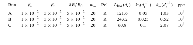


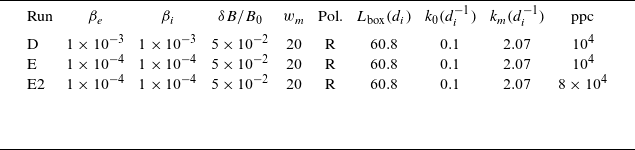


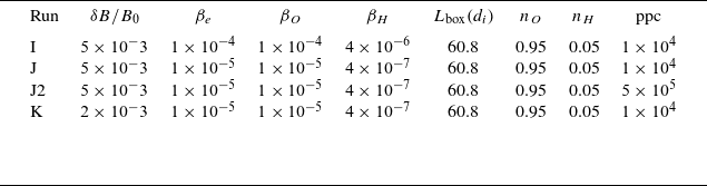


 Open access