





1 Introduction
Consider a continuous map $F: X\to X$
on a metric space X, equipped with a probability (reference) measure
$F: X\to X$
on a metric space X, equipped with a probability (reference) measure $\mu $
. A closed subset
$\mu $
. A closed subset $A \subset X$
will be called a metric attractor of F if it satisfies two conditions:
$A \subset X$
will be called a metric attractor of F if it satisfies two conditions:
-
(1) the basin of attraction
has positive measure $$ \begin{align*} \rho(A) := \{ x \in X; \omega(x) \subset A \} \end{align*} $$
$\mu (\rho (A))>0$
;
$$ \begin{align*} \rho(A) := \{ x \in X; \omega(x) \subset A \} \end{align*} $$
$\mu (\rho (A))>0$
;
-
(2) there is no strictly smaller closed set
$A' \subset A$
so that
$\rho (A')$
coincides with
$\rho (A)$
up to a set of measure zero.




The basin of attraction is not required to be an open set. This notion of attractor was coined by Milnor [Reference Milnor28] to have a definition that is less restrictive than topological definitions making use of asymptotic stability. One also finds the term Milnor attractor in the literature. A metric attractor is called a minimal (metric) attractor if moreover:
-
(3) there is no strictly smaller closed set
$A'\subset A$
for which
$\rho (A')$
has positive measure.


We also adopt from [Reference Milnor28] the definition of likely limit set A of F as the smallest closed subset of X with the property that $\omega (x) \subset A$
for every point
$\omega (x) \subset A$
for every point $x \in X$
outside of a set of measure zero.
$x \in X$
outside of a set of measure zero.
The basins of attraction of two attractors $A_1$
and
$A_1$
and $A_2$
are said to be intermingled basins of attraction if they are measure theoretically dense in each other: if one basin meets an open set U in a set of positive measure, then also the other basin meets U in a set of positive measure [Reference Alexander, Yorke, You and Kan1]. A key example of a system with intermingled metric attractors is due to Kan [Reference Kan25]. It involves a smooth map on the annulus
$A_2$
are said to be intermingled basins of attraction if they are measure theoretically dense in each other: if one basin meets an open set U in a set of positive measure, then also the other basin meets U in a set of positive measure [Reference Alexander, Yorke, You and Kan1]. A key example of a system with intermingled metric attractors is due to Kan [Reference Kan25]. It involves a smooth map on the annulus $\mathbb {T} \times [0,1]$
that fixes the boundaries
$\mathbb {T} \times [0,1]$
that fixes the boundaries $\mathbb {T} \times \{0\}$
and
$\mathbb {T} \times \{0\}$
and $\mathbb {T} \times \{1\}$
. The boundaries in this example are metric attractors. An explicit expression for such a map is
$\mathbb {T} \times \{1\}$
. The boundaries in this example are metric attractors. An explicit expression for such a map is
 $$ \begin{align*} (u,x) \mapsto \bigg(3 u \pmod 1 , x + \frac{\cos(2 \pi u)}{32} x (1-x) \bigg). \end{align*} $$
Various other constructions have been provided in the literature, for instance [Reference Bonatti and Potrie7, Reference Bonifant and Milnor8, Reference Fayad13, Reference Melbourne and Windsor27]. Examples of the occurrence of attractors with intermingled basins in models are in [Reference Camargo, Viana and Anteneodo9, Reference Hofbauer, Hofbauer, Raith and Steinberger17, Reference Homburg, Jamilov and Scheutzow18].
To address measure theoretical aspects of Kan’s example, we need two more notions. Recall first that for an ergodic invariant measure $\nu $
of F, the basin of
$\nu $
of F, the basin of $\nu $
is defined by
$\nu $
is defined by
 $$ \begin{align*} \rho(\nu) := \bigg\{x\in X; \lim_{n\to \infty}\frac{1}{n}\sum_{i=0}^{n-1}\delta_{F^i(x)}\rightarrow\nu\bigg\}, \end{align*} $$
with convergence in the weak star topology and where $\delta _x$
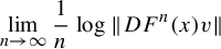
stands for the atomic measure at x. For the second notion, we need that X is a smooth manifold and F is a smooth map defined on it. By the classical Oseledec’s theorem, if
$\delta _x$
stands for the atomic measure at x. For the second notion, we need that X is a smooth manifold and F is a smooth map defined on it. By the classical Oseledec’s theorem, if $\nu $
is an ergodic F-invariant measure, then for
$\nu $
is an ergodic F-invariant measure, then for $\nu $
-almost every (a.e.)
$\nu $
-almost every (a.e.) $x\in X$
and any vector v belonging to the tangent space
$x\in X$
and any vector v belonging to the tangent space $T_x X$
, the limits
$T_x X$
, the limits
 $$ \begin{align*}\lim_{n\to\infty} \frac{1}{n} \log \|DF^n(x)v\|\end{align*} $$
exist. The measure $\nu $
is called hyperbolic if the above limits are all non-zero.
$\nu $
is called hyperbolic if the above limits are all non-zero.
In Kan’s example, the Lebesgue measures on the two boundary circles are ergodic invariant measures with positive horizontal and negative vertical Lyapunov exponents. The negative Lyapunov exponents guarantee that the basins have positive volume. The supports of both measures have zero volume, as they are supported on the boundary circles. In particular, these two measures are singular with respect to the volume on $\mathbb {T}\times [0,1]$
. Now, a question arises.
$\mathbb {T}\times [0,1]$
. Now, a question arises.
Question. Is there a dynamical system with two attractors with hyperbolic ergodic absolutely continuous invariant measures whose basins are intermingled in some open set?
There are obstacles for an example in the context of partially hyperbolic dynamics. For instance, in [Reference Ures and Vásquez32], the authors prove that each ergodic invariant measure of a partially hyperbolic diffeomorphism on $\mathbb {T}^3$
with intermingled basins is supported on a two-dimensional torus and so it cannot be absolutely continuous. In this context, we also have the stable and unstable saturation of dynamics on the support of an absolutely continuous measure as a crucial obstacle (see [Reference Zhang35]). In contrast, using the Anosov–Katok method, the author in [Reference Fayad, Brin, Hasselblatt and Pesin14] provides an example of a
$\mathbb {T}^3$
with intermingled basins is supported on a two-dimensional torus and so it cannot be absolutely continuous. In this context, we also have the stable and unstable saturation of dynamics on the support of an absolutely continuous measure as a crucial obstacle (see [Reference Zhang35]). In contrast, using the Anosov–Katok method, the author in [Reference Fayad, Brin, Hasselblatt and Pesin14] provides an example of a $C^\infty $
diffeomorphism with two intermingled basins but with one hyperbolic component (open and dense basin) and the other having zero exponent.
$C^\infty $
diffeomorphism with two intermingled basins but with one hyperbolic component (open and dense basin) and the other having zero exponent.
The above question is a motivation for us to consider a class of attractors, called thick metric attractors, that have the potential to be the support of absolutely continuous measures. A metric attractor A is thick if $0 < \mu (A) < 1$
, so A has positive but not full measure. This phenomenon of a thick attractor has been described by Ilyashenko in [Reference Ilyashenko21] who gave constructions for skew product systems over shifts, arising from iterated function systems, and later in [Reference Ilyashenko22] also for diffeomorphisms.
$0 < \mu (A) < 1$
, so A has positive but not full measure. This phenomenon of a thick attractor has been described by Ilyashenko in [Reference Ilyashenko21] who gave constructions for skew product systems over shifts, arising from iterated function systems, and later in [Reference Ilyashenko22] also for diffeomorphisms.
Here, we begin by presenting fundamental ideas for creating attractors with intermingled basins. One of the main yet simple ideas is random walks along orbits of a given dynamical system. Random walks along orbits appeared in [Reference Conze and Guivarch11, Reference Kaloshin and Sinai23, Reference Kaloshin and Sinai24, Reference Sinai31] that looked at contexts of ergodic measure-preserving automorphisms. One setting is that of a diffeomorphism f, where random walks along orbits amount to
 $$ \begin{align*} x_{n+1} := f^{\eta_n} (x_n) \end{align*} $$
for steps $\eta _n = \pm 1$
. We will allow the distribution of the steps
$\eta _n = \pm 1$
. We will allow the distribution of the steps $\eta _n$
to be position dependent, that is, depending on
$\eta _n$
to be position dependent, that is, depending on $x_n$
. For a flow
$x_n$
. For a flow $x(t) = \varphi (t,x_0)$
of a differential equation, we will look at
$x(t) = \varphi (t,x_0)$
of a differential equation, we will look at
 $$ \begin{align*} x(t) = \varphi (s_t , x_0), \end{align*} $$
where $s_t$
is a random process on
$s_t$
is a random process on $\mathbb {R}$
.
$\mathbb {R}$
.
We rewrite such random systems as deterministic systems to give novel and elementary constructions of attractors with intermingled basins. Then, we will use the large freedom for which the constructions allow to provide examples of thick metric attractors with intermingled basins. Finally, we describe how this strategy can lead to the creation of multiple metric attractors with intermingled basins.
2 Elementary examples of intermingled basins
We present different but related constructions of dynamics with metric attractors and intermingled basins. We start with definitions of spaces and maps, also to fix notation. Random binary choices are modeled by shifts on sequences of symbols. For this, we denote
 $$ \begin{align} \Sigma_2^+ &:= \{0,1\}^{\mathbb{N}}, \end{align} $$
equipped with the product topology. Elements of $\Sigma _2^+$
are written as
$\Sigma _2^+$
are written as $\omega = (\omega _i)_{i\in \mathbb {N}}$
. The left shift operator
$\omega = (\omega _i)_{i\in \mathbb {N}}$
. The left shift operator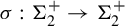 $\sigma : \Sigma _2^+ \to \Sigma _2^+$
is given by
$\sigma : \Sigma _2^+ \to \Sigma _2^+$
is given by $(\sigma \omega )_i = \omega _{i+1}$
. We write
$(\sigma \omega )_i = \omega _{i+1}$
. We write $[a_0,\ldots ,a_k]$
for the cylinder
$[a_0,\ldots ,a_k]$
for the cylinder
 $$ \begin{align*} [a_0,\ldots,a_k] := \{ \omega \in \Sigma_2^+; \omega_i = a_i, 0\le i \le k\}. \end{align*} $$
The number $k+1$
of fixed symbols is the depth of the cylinder. For two cylinders,
$k+1$
of fixed symbols is the depth of the cylinder. For two cylinders, $C := [a_0,\ldots ,a_k]$
and
$C := [a_0,\ldots ,a_k]$
and $D := [b_0,\ldots ,b_l]$
, we write
$D := [b_0,\ldots ,b_l]$
, we write $C \, D := [a_0,\ldots ,a_k,b_0,\ldots ,b_l]$
. Bernoulli measure
$C \, D := [a_0,\ldots ,a_k,b_0,\ldots ,b_l]$
. Bernoulli measure $\nu _p$
corresponding to a probability p for the symbol
$\nu _p$
corresponding to a probability p for the symbol $0$
and
$0$
and $1-p$
for the symbol
$1-p$
for the symbol $1$
is determined by defining it on cylinder sets as
$1$
is determined by defining it on cylinder sets as
 $$ \begin{align*} \nu_p ([a_0,\ldots,a_k]) := p^{\# \{i; 0\le i \le k, a_i = 0\} } (1-p)^{{\# \{i; 0\le i \le k, a_i = 1\} }}. \end{align*} $$
For two-sided sequences, we write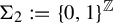 $\Sigma _2 := \{0,1\}^{\mathbb {Z}}$
, taking away the superscript ‘+’.
$\Sigma _2 := \{0,1\}^{\mathbb {Z}}$
, taking away the superscript ‘+’.
Recall that two maps  and
and  that preserve probability measures $\mu $
and
$\mu $
and $\nu $
are measurably isomorphic if there is a measure preserving bijection
$\nu $
are measurably isomorphic if there is a measure preserving bijection $H: X' \to Y'$
between invariant subsets
$H: X' \to Y'$
between invariant subsets $X' \subset X$
and
$X' \subset X$
and $Y' \subset Y$
of full measure so that
$Y' \subset Y$
of full measure so that $H \circ F = G \circ H$
, see [Reference Einsiedler and Ward12, Definition 2.7]. From the correspondence between binary expansions of numbers in the unit interval and symbol sequences in
$H \circ F = G \circ H$
, see [Reference Einsiedler and Ward12, Definition 2.7]. From the correspondence between binary expansions of numbers in the unit interval and symbol sequences in $\Sigma _2$
, one gets that the shift on
$\Sigma _2$
, one gets that the shift on $\Sigma _2^+$
with Bernoulli measure
$\Sigma _2^+$
with Bernoulli measure $\nu _p$
is measurably isomorphic to the piecewise linear map
$\nu _p$
is measurably isomorphic to the piecewise linear map $E_p: [0,1] \to [0,1]$
with Lebesgue measure, where
$E_p: [0,1] \to [0,1]$
with Lebesgue measure, where $E_p$
is given by
$E_p$
is given by
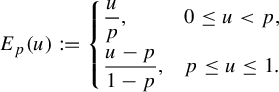 $$ \begin{align*} E_p (u) &:= \begin{cases} \dfrac{u}{p}, & 0 \le u < p, \\[6pt] \dfrac{u-p}{1-p}, & p \le u \le 1. \end{cases} \end{align*} $$
Note that indeed, $E_p$
leaves the Lebesgue measure on
$E_p$
leaves the Lebesgue measure on $[0,1]$
invariant. Likewise, the shift on
$[0,1]$
invariant. Likewise, the shift on $\Sigma _2$
endowed with Bernoulli measure
$\Sigma _2$
endowed with Bernoulli measure $\nu _{p}$
is measurably isomorphic to the two-dimensional baker’s map
$\nu _{p}$
is measurably isomorphic to the two-dimensional baker’s map $B_p$
on
$B_p$
on $[0,1)^2$
given by
$[0,1)^2$
given by
 $$ \begin{align} B_p(w,y) &:= \begin{cases} \bigg(\dfrac{w}{p} , p y \bigg), & 0\le w < p, \\[6pt] \bigg(\dfrac{w}{1-p} - \dfrac{p}{1-p} , (1-p) y + p \bigg), & p \le w < 1, \end{cases} \end{align} $$
and endowed with Lebesgue measure.
We will use the single symbol $\unicode{x3bb} $
to denote Lebesgue measure on the interval
$\unicode{x3bb} $
to denote Lebesgue measure on the interval $[0,1]$
or the circle
$[0,1]$
or the circle $\mathbb {T}$
. We also write
$\mathbb {T}$
. We also write $\unicode{x3bb} $
for Lebesgue measure on higher dimensional intervals
$\unicode{x3bb} $
for Lebesgue measure on higher dimensional intervals $[0,1]^d$
and tori
$[0,1]^d$
and tori $\mathbb {T}^d$
.
$\mathbb {T}^d$
.
2.1 Random walks on orbits of diffeomorphisms: position dependent probabilities
Consider a compact manifold N and a diffeomorphism  . Let
. Let $p:N \to (0,1)$
be a continuous function. For a given initial point
$p:N \to (0,1)$
be a continuous function. For a given initial point $x_0 \in N$
, take a random walk
$x_0 \in N$
, take a random walk
 $$ \begin{align} x_{n+1} &:= f^{\eta_n} (x_n) \end{align} $$
along the orbit of $x_0$
, where
$x_0$
, where $\eta _n = \pm 1$
for
$\eta _n = \pm 1$
for $n \in \mathbb {Z}$
is taken independently with probabilities
$n \in \mathbb {Z}$
is taken independently with probabilities $p(x_n)$
for the value
$p(x_n)$
for the value $+1$
and
$+1$
and $1-p(x_n)$
for the value
$1-p(x_n)$
for the value $-1$
. One can view this as random walks in environments on
$-1$
. One can view this as random walks in environments on $\mathbb {Z}$
, where an environment stands for a choice of probabilities on points in
$\mathbb {Z}$
, where an environment stands for a choice of probabilities on points in $\mathbb {Z}$
with which possible steps are taken [Reference Chung10]. Perturbations of initial points can then give different environments. We get
$\mathbb {Z}$
with which possible steps are taken [Reference Chung10]. Perturbations of initial points can then give different environments. We get $x_n = x_n(\eta )$
as a function of
$x_n = x_n(\eta )$
as a function of $\eta = (\eta _i)_{i\in \mathbb {Z}}$
.
$\eta = (\eta _i)_{i\in \mathbb {Z}}$
.
We will write the above random walk as a skew product system over a shift. Instead of taking two symbols $0$
and
$0$
and $1$
as in (2.1), we find it convenient to use symbols
$1$
as in (2.1), we find it convenient to use symbols $-1$
and
$-1$
and $+1$
and write
$+1$
and write
 $$ \begin{align*} \Omega^+ &= \{-1,+1\}^{\mathbb{N}}. \end{align*} $$
Other notation such as for the shift operator and cylinders will be as before. Define the skew product map  by
by
 $$ \begin{align} G(\eta , x) &:= (\sigma \eta , f^{\eta_0} (x) ). \end{align} $$
For iterates, we use the notation
 $$ \begin{align} G^n (\eta,x) &= (\sigma^n \eta , f^{S_n (\eta)} (x) ) \quad\text{with } S_n(\eta) := \sum_{i=0}^{n-1} \eta_i. \end{align} $$
Write $p_{-1} (x) := 1 - p (x)$
and
$p_{-1} (x) := 1 - p (x)$
and $p_{1} (x) := p(x)$
. Let
$p_{1} (x) := p(x)$
. Let $\zeta _x$
be the measure on
$\zeta _x$
be the measure on $\Omega ^+$
which is defined on cylinders by
$\Omega ^+$
which is defined on cylinders by
 $$ \begin{align} \zeta_x ([a_0\cdots a_k]) &:= \prod_{i=0}^k p_{a_i} (f^{S_i (a)} (x)). \end{align} $$
In words, $\zeta _x([a_0\cdots a_k])$
equals the probability for the random walk starting at x to walk through
$\zeta _x([a_0\cdots a_k])$
equals the probability for the random walk starting at x to walk through $x, f^{a_0} (x), f^{a_0+a_1} (x),\ldots ,f^{a_0 + \cdots + a_k}(x)$
. By the Hahn–Kolmogorov extension theorem, (2.6) defines the measure
$x, f^{a_0} (x), f^{a_0+a_1} (x),\ldots ,f^{a_0 + \cdots + a_k}(x)$
. By the Hahn–Kolmogorov extension theorem, (2.6) defines the measure $\zeta _x$
on the Borel
$\zeta _x$
on the Borel $\sigma $
-algebra on
$\sigma $
-algebra on $\Omega ^+$
. For a measure m on N, define the measure
$\Omega ^+$
. For a measure m on N, define the measure $\mu _m$
on
$\mu _m$
on $\Omega ^+ \times N$
by
$\Omega ^+ \times N$
by

where $A_x := A \cap (\Omega ^+ \times \{x\})$
. As p is continuous, we find that
$A_x := A \cap (\Omega ^+ \times \{x\})$
. As p is continuous, we find that $\zeta _x$
depends continuously on x in the weak star topology.
$\zeta _x$
depends continuously on x in the weak star topology.
A Borel measure m on N is stationary if
 $$ \begin{align} m(I) &= \int_{f^{-1} (I)} p_1 (x) \, dm (x) + \int_{f (I)} p_{-1} (x) \, dm (x). \end{align} $$
A theory of deterministic representations for the random system (2.3) is developed in [Reference Bahsoun, Bose and Quas3], relating stationary measures to invariant measures of a certain deterministic system defined on $[0,1]\times N$
. Our approach centers around the skew product system G, and has the following correspondence result between stationary measures and invariant measures for G. Although formulated for the specific setup of iterated function systems generated by f and
$[0,1]\times N$
. Our approach centers around the skew product system G, and has the following correspondence result between stationary measures and invariant measures for G. Although formulated for the specific setup of iterated function systems generated by f and $f^{-1}$
, our approach is not restricted to this setup and works more generally for iterated function systems with position dependent probabilities. Although stationary measures do not play a vital role in the constructions in this paper, the following result, see also [Reference Barnsley, Demko, Elton and Geronimo4], is included as it clarifies the setup.
$f^{-1}$
, our approach is not restricted to this setup and works more generally for iterated function systems with position dependent probabilities. Although stationary measures do not play a vital role in the constructions in this paper, the following result, see also [Reference Barnsley, Demko, Elton and Geronimo4], is included as it clarifies the setup.
Proposition 2.1. A probability measure m is stationary for the Markov process if and only if $\mu _m$
is invariant for G.
$\mu _m$
is invariant for G.
Proof. We first prove that if $\mu _m$
is invariant for G, then m is stationary. Consider a product set
$\mu _m$
is invariant for G, then m is stationary. Consider a product set $A = C \times I$
of a cylinder C and a Borel set I. By definition of the measures
$A = C \times I$
of a cylinder C and a Borel set I. By definition of the measures $\zeta _x$
, we have
$\zeta _x$
, we have
 $$ \begin{align}\begin{aligned} \zeta_{x} (-1\, C) &= p_{-1} (x) \zeta_{f^{-1}(x)} ( C ), \\ \zeta_{x} (1\, C) &= p_1 (x) \zeta_{f(x)} ( C ). \end{aligned}\end{align} $$
Calculate
 $$ \begin{align*} \mu_m (G^{-1} (A)) &= \int_{f^{-1} (I)} \zeta_{x} (1\, C) \, dm (x) + \int_{f (I)} \zeta_{x} (-1\, C) \, dm (x) \\ &= \int_{f^{-1} (I)} p_1 (x) \zeta_{f(x)} ( C ) \, dm (x) + \int_{f (I)} p_{-1} (x) \zeta_{f^{-1}(x)} ( C ) \, dm (x) \end{align*} $$
and note
 $$ \begin{align*} \mu_m (A) &= \int_I \zeta_x (C) \, dm (x). \end{align*} $$
By invariance of $\mu _m$
, these expressions are equal. Apply this to
$\mu _m$
, these expressions are equal. Apply this to $C = \Omega ^+$
. Then,
$C = \Omega ^+$
. Then,
 $$ \begin{align*} m(I) &= \int_{f^{-1} (I)} p_1 (x)\, dm (x) + \int_{f (I)} p_{-1} (x) \, dm (x), \end{align*} $$
which means that m is stationary.
For the other direction, let $A := C \times I$
be a product set in
$A := C \times I$
be a product set in $\Omega ^+ \times N$
as above and suppose m is a stationary probability measure. Write (2.8) as
$\Omega ^+ \times N$
as above and suppose m is a stationary probability measure. Write (2.8) as

Approximating an arbitrary integrable function $\psi $
by step functions, we get from this
$\psi $
by step functions, we get from this
 $$ \begin{align} \int \psi (x)\, dm (x) &= \int \psi (f (x) ) p_1 (x) \, dm (x) + \int \psi (f^{-1}(x)) p_{-1} (x) \, dm (x). \end{align} $$
Using (2.9), calculate

Choosing  , we get from (2.10) that the last line equals

which is $\mu _m(A)$
. So,
$\mu _m(A)$
. So,
 $$ \begin{align*} \mu_m (G^{-1}(A)) = \mu_m (A), \end{align*} $$
which proves invariance of $\mu _m$
since these product sets generate the Borel
$\mu _m$
since these product sets generate the Borel $\sigma $
-algebra.
$\sigma $
-algebra.
2.1.1 North pole/south pole diffeomorphisms on the circle
We specialize the above construction to a north pole/south pole diffeomorphism f on a circle $\mathbb {S}^{1}$
. This gives a prototype example of metric attractors with intermingled basins. The north pole
$\mathbb {S}^{1}$
. This gives a prototype example of metric attractors with intermingled basins. The north pole $p_N$
is a repelling fixed point for f and the south pole
$p_N$
is a repelling fixed point for f and the south pole $p_S$
an attracting fixed point. The basin of attraction of
$p_S$
an attracting fixed point. The basin of attraction of $p_S$
is
$p_S$
is $\mathbb {S}^{1} \setminus \{p_N\}$
.
$\mathbb {S}^{1} \setminus \{p_N\}$
.
Assume the function p satisfies
 $$ \begin{align} p (p_S)> 1/2, \quad p(p_N) < 1/2. \end{align} $$
As before, denote Lebesgue measure on the circle by $\unicode{x3bb} $
. The measure
$\unicode{x3bb} $
. The measure $\mu _\unicode{x3bb} $
on
$\mu _\unicode{x3bb} $
on $\Omega ^+ \times \mathbb {S}^1$
is then defined as in (2.7).
$\Omega ^+ \times \mathbb {S}^1$
is then defined as in (2.7).
Theorem 2.2. Let the continuous function $p:\mathbb {S}^1 \to (0,1)$
satisfy (2.11) and take
$p:\mathbb {S}^1 \to (0,1)$
satisfy (2.11) and take $\Omega ^+ \times \mathbb {S}^1$
endowed by the reference measure
$\Omega ^+ \times \mathbb {S}^1$
endowed by the reference measure $\mu _\unicode{x3bb} $
. Consider the dynamical system on
$\mu _\unicode{x3bb} $
. Consider the dynamical system on $\Omega ^+ \times \mathbb {S}^1$
given by (2.4). Then,
$\Omega ^+ \times \mathbb {S}^1$
given by (2.4). Then, $\Omega ^+ \times \{p_N\}$
and
$\Omega ^+ \times \{p_N\}$
and $\Omega ^+ \times \{p_S\}$
are metric attractors with intermingled basins. The union
$\Omega ^+ \times \{p_S\}$
are metric attractors with intermingled basins. The union $\Omega ^+ \times \{p_N,p_S\}$
is the likely limit set.
$\Omega ^+ \times \{p_N,p_S\}$
is the likely limit set.
Proof. Consider an orbit $x_{n+1} := f(x_n)$
. Identifying
$x_{n+1} := f(x_n)$
. Identifying $x_n$
with n, the random walk (2.3) gives a random walk on
$x_n$
with n, the random walk (2.3) gives a random walk on $\mathbb {Z}$
. The statements follow from the theory of random walks in environments, see [Reference Chung10, §I.12] and [Reference Little26, §2.2]. For every
$\mathbb {Z}$
. The statements follow from the theory of random walks in environments, see [Reference Chung10, §I.12] and [Reference Little26, §2.2]. For every $x \in \mathbb {S}^1 \setminus \{p_S,p_N\}$
, there is a
$x \in \mathbb {S}^1 \setminus \{p_S,p_N\}$
, there is a $P(x) \in (0,1)$
so that the probability of converging to
$P(x) \in (0,1)$
so that the probability of converging to $p_S$
equals
$p_S$
equals $P(x)$
and the probability of converging to
$P(x)$
and the probability of converging to $p_N$
is
$p_N$
is $1-P(x)$
. This means that
$1-P(x)$
. This means that
 $$ \begin{align*} \zeta_x \Big(\Big\{\eta \in \Omega^+; \lim_{n\to \infty} f^{S_n(\eta)}(x) = p_S \Big\}\Big) &= P(x),\\ \zeta_x \Big(\Big\{\eta \in \Omega^+; \lim_{n\to \infty} f^{S_n(\eta)} (x) = p_N \Big\}\Big) &= 1 - P(x), \end{align*} $$
where S is defined as in (2.5). So, the basins of attraction $\rho (\Omega ^+ \times \{p_S\})$
and
$\rho (\Omega ^+ \times \{p_S\})$
and $\rho (\Omega ^+ \times \{p_N\})$
satisfy
$\rho (\Omega ^+ \times \{p_N\})$
satisfy
 $$ \begin{align*} \zeta_x (\rho (\Omega^+ \times \{p_S\}) \cap (\Omega^+ \times \{x\})) &= P (x), \\ \zeta_x (\rho (\Omega^+ \times \{p_N\}) \cap (\Omega^+ \times \{x\})) &= 1-P (x). \end{align*} $$
Let U be an open set in $\Omega ^+ \times \mathbb {S}^1$
. Take a product set
$\Omega ^+ \times \mathbb {S}^1$
. Take a product set $C \times I \subset U$
of a cylinder C and an open interval
$C \times I \subset U$
of a cylinder C and an open interval $I \subset S^1$
. If C has depth k, then the iterate
$I \subset S^1$
. If C has depth k, then the iterate $G^k ( C \times I)$
will be of the form
$G^k ( C \times I)$
will be of the form $\Omega ^+ \times I_k$
for an open interval
$\Omega ^+ \times I_k$
for an open interval $I_k$
. This gives
$I_k$
. This gives
 $$ \begin{align*} \mu_\unicode{x3bb}(\rho(\Omega^+ \times \{p_S\}) \cap \Omega^+ \times I_k ) &= \int_{I_k} P(x) \, d\unicode{x3bb} (x)> 0, \\ \mu_\unicode{x3bb}(\rho(\Omega^+ \times \{p_N\}) \cap \Omega^+ \times I_k) &= \int_{I_k} 1 - P(x) \, d\unicode{x3bb}(x) (x)> 0. \end{align*} $$
So also both $ \mu _\unicode{x3bb} ( U \cap \rho (\Omega ^+ \times \{p_S\}))> 0$
and
$ \mu _\unicode{x3bb} ( U \cap \rho (\Omega ^+ \times \{p_S\}))> 0$
and $\mu _\unicode{x3bb} ( U \cap \rho (\Omega ^+ \times \{p_N\}))> 0$
. This proves the statements.
$\mu _\unicode{x3bb} ( U \cap \rho (\Omega ^+ \times \{p_N\}))> 0$
. This proves the statements.
2.2 Skew product systems
We continue with elementary constructions of intermingled basins somewhat in the spirit of Kan’s example [Reference Kan25], but using random walks on orbits of flows on compact manifolds.
Consider the flow of a Morse–Smale gradient differential equation
 $$ \begin{align} \dot{x} &= g(x) \end{align} $$
on a compact manifold N. We have
 $$ \begin{align} g &= -\text{grad}\, (h) \end{align} $$
with a height function $h : N \to [0,1]$
. See for instance [Reference Palis and de Melo30] for background. We assume that (2.12) has a unique attracting equilibrium
$h : N \to [0,1]$
. See for instance [Reference Palis and de Melo30] for background. We assume that (2.12) has a unique attracting equilibrium $p_S$
and a unique repelling equilibrium
$p_S$
and a unique repelling equilibrium $p_N$
. Such flows exist on any compact manifold. We can assume
$p_N$
. Such flows exist on any compact manifold. We can assume $h(p_S) = 1$
and
$h(p_S) = 1$
and $h (p_N)=0$
. Note that flows that provide north pole/south pole diffeomorphisms on the circle or on a sphere are possible examples. Write
$h (p_N)=0$
. Note that flows that provide north pole/south pole diffeomorphisms on the circle or on a sphere are possible examples. Write $\varphi _t: N \to N$
for the flow of (2.12). We will also write
$\varphi _t: N \to N$
for the flow of (2.12). We will also write $\varphi (t,x) := \varphi _t (x)$
.
$\varphi (t,x) := \varphi _t (x)$
.
Let $E: \mathbb {T} \to \mathbb {T}$
(here,
$E: \mathbb {T} \to \mathbb {T}$
(here, $\mathbb {T} := \mathbb {R}/\mathbb {Z}$
) be an expanding map
$\mathbb {T} := \mathbb {R}/\mathbb {Z}$
) be an expanding map $E (u) := L u \pmod 1$
for some integer
$E (u) := L u \pmod 1$
for some integer $L> 2$
. Let
$L> 2$
. Let $s : \mathbb {T} \times N \to \mathbb {R}$
be a smooth scalar function satisfying the following properties.
$s : \mathbb {T} \times N \to \mathbb {R}$
be a smooth scalar function satisfying the following properties.
-
(1) There are fixed points
$q_1, q_2$
for E so that for all
$x \in N$
,
$$ \begin{align*} s(q_1,x) <0, \quad s(q_2,x)>0. \end{align*} $$
-
(2) We have
$$ \begin{align*} \int_{\mathbb{T}} s(u,p_N) \, du < 0, \quad \int_{\mathbb{T}} s(u,p_S) \, du> 0. \end{align*} $$


By compactness of N, there is $C>0$
so that for all
$C>0$
so that for all $x \in N$
,
$x \in N$
, $s(q_1,x) < -C < 0$
and
$s(q_1,x) < -C < 0$
and $s(q_2,x)> C > 0$
. An example of a system with the above conditions is obtained by taking a smooth scalar function
$s(q_2,x)> C > 0$
. An example of a system with the above conditions is obtained by taking a smooth scalar function $\eta : \mathbb {T} \to \mathbb {R}$
satisfying
$\eta : \mathbb {T} \to \mathbb {R}$
satisfying
 $$ \begin{align*} \int_{\mathbb{T}}\eta (u) \, du = 0, \quad \eta (q_1) < 0, \; \eta(q_2)>0, \end{align*} $$
and then letting
 $$ \begin{align*} s (u,x) := \eta(u) + \delta (h(x) - \tfrac{1}{2}) \end{align*} $$
for some small $\delta>0$
.
$\delta>0$
.
Consider the skew product system  given by
 $$ \begin{align} F(u,x) &:= ( E (u) , \varphi_{s(u,x)} (x)). \end{align} $$
Write this as
 $$ \begin{align*} F(u,x) = ( E (u) , f_u (x)) \end{align*} $$
and denote iterates as
 $$ \begin{align*} F^n(u,x) = ( E^n (u) , f^n_u (x)). \end{align*} $$
Note $f^n_u(x) = \varphi _{s_n(u,x)} (x)$
with
$f^n_u(x) = \varphi _{s_n(u,x)} (x)$
with
 $$ \begin{align*} s_n(u,x) := \sum_{i=0}^{n-1} s(E^i (u) , f^i_u(x) ). \end{align*} $$
The top fiber Lyapunov exponent $L_{p_S} := \lim _{n\to \infty } ({1}/{n}) \ln (\| Df^n_u (p_S)\|)$
at
$L_{p_S} := \lim _{n\to \infty } ({1}/{n}) \ln (\| Df^n_u (p_S)\|)$
at $p_S$
exists for Lebesgue almost all
$p_S$
exists for Lebesgue almost all $u\in \mathbb {T}$
. Applying Birkhoff’s ergodic theorem, one gets
$u\in \mathbb {T}$
. Applying Birkhoff’s ergodic theorem, one gets
 $$ \begin{align*} \lim_{n\to \infty} \frac{1}{n} \sum_{i=0}^{n-1} s (E^i(u),p_S) = \int_{\mathbb{T}} s (u , p_S)\, du> 0. \end{align*} $$
Using this in the linearized flow $v\mapsto D \varphi _{s(u,p_S)} (p_S) v = e^{ Dg(p_S) s(u,p_S) }v $
shows
$v\mapsto D \varphi _{s(u,p_S)} (p_S) v = e^{ Dg(p_S) s(u,p_S) }v $
shows
 $$ \begin{align*} L_{p_S} = \lim_{n\to \infty} \frac{1}{n} \ln ( \| e^{Dg (p_S) n} \| ) = \int_{\mathbb{T}} s (u , p_S)\, du < 0. \end{align*} $$
Here, $\lim _{n\to \infty } ({1}/{n}) \ln ( \| e^{Dg (p_S) n} \| ) $
is the top Lyapunov exponent of the flow
$\lim _{n\to \infty } ({1}/{n}) \ln ( \| e^{Dg (p_S) n} \| ) $
is the top Lyapunov exponent of the flow $v\mapsto D \varphi _{t} (p_S) v = e^{ Dg(p_S) t }v$
. Likewise, we have a negative top fiber Lyapunov exponent at
$v\mapsto D \varphi _{t} (p_S) v = e^{ Dg(p_S) t }v$
. Likewise, we have a negative top fiber Lyapunov exponent at $p_N$
.
$p_N$
.
Theorem 2.3. Consider the skew product system F from (2.14) on $\mathbb {T} \times N$
. Take volume on
$\mathbb {T} \times N$
. Take volume on $\mathbb {T} \times N$
as reference measure. The sets
$\mathbb {T} \times N$
as reference measure. The sets $\mathbb {T} \times \{p_N\}$
and
$\mathbb {T} \times \{p_N\}$
and $\mathbb {T} \times \{ p_S\}$
are minimal metric attractors with intermingled basins. The union
$\mathbb {T} \times \{ p_S\}$
are minimal metric attractors with intermingled basins. The union $\mathbb {T} \times \{p_N,p_S\}$
is the likely limit set.
$\mathbb {T} \times \{p_N,p_S\}$
is the likely limit set.
Proof. For $\delta $
positive, write
$\delta $
positive, write $B_\delta (p_S)$
for the
$B_\delta (p_S)$
for the $\delta $
-neighborhood of
$\delta $
-neighborhood of $p_S$
. For
$p_S$
. For $\delta $
sufficiently small, say
$\delta $
sufficiently small, say $\delta \le \delta _0$
,
$\delta \le \delta _0$
, $B_\delta (p_S)$
will be a ball. Let
$B_\delta (p_S)$
will be a ball. Let $\unicode{x3bb} <0$
be such that the spectrum of
$\unicode{x3bb} <0$
be such that the spectrum of $Dg (p_S)$
is contained in
$Dg (p_S)$
is contained in $\{ z \in \mathbb {C}; \text {Re}\, (z) < \unicode{x3bb} \}$
. Standard estimates on solutions of differential equations near equilibria show that for orbits
$\{ z \in \mathbb {C}; \text {Re}\, (z) < \unicode{x3bb} \}$
. Standard estimates on solutions of differential equations near equilibria show that for orbits $f^n_u(x)$
that stay inside
$f^n_u(x)$
that stay inside $B_\delta (p_S)$
, so
$B_\delta (p_S)$
, so $f^i_u(x) \in B_\delta (p_S)$
for
$f^i_u(x) \in B_\delta (p_S)$
for $0\le i \le n$
, we have a bound
$0\le i \le n$
, we have a bound
 $$ \begin{align*} d(f^n_u (x), p_S) &= d ( \varphi_{ s(E^n(u) , f^{n-1}_{E^n(u)} (x))} (f^{n-1}_{E^n(u)} (x)) \circ \cdots \circ \varphi_{s(u,x)} (x) ,p_S)\\ &\le C e^{\unicode{x3bb} \,s_n (u,p_S)} d(x,p_S) \end{align*} $$
for some $C>0$
. The function
$C>0$
. The function
 $$ \begin{align*} r (u) = \sup \Big\{ \delta; \delta \le \delta_0, f^n_u (x_0) \in B_{\delta_0} (p_S) \text{ for } n \ge 0, \lim_{n\to\infty} f^n_u (x_0) = p_S \Big\} \end{align*} $$
is therefore positive for Lebesgue almost all u. Compare the exposition of Pesin theory in [Reference Barreira and Pesin5] and the direct estimates as in [Reference Gharaei and Homburg15, Lemma 3.1], [Reference Kan25, Lemma 2.2], or [Reference Bonifant and Milnor8, Lemma A.1]. We thus find local stable manifolds $\{u\} \times U_u \subset \{u\} \times N$
of
$\{u\} \times U_u \subset \{u\} \times N$
of $(u,p_S)$
for Lebesgue almost all u. More precisely,
$(u,p_S)$
for Lebesgue almost all u. More precisely, $x_0 \in U_u$
means that
$x_0 \in U_u$
means that $F^n (u,x_0) \in \mathbb {T}\times B_{\delta _0} (p_S)$
for all
$F^n (u,x_0) \in \mathbb {T}\times B_{\delta _0} (p_S)$
for all $n \ge 0$
, and hence the
$n \ge 0$
, and hence the $\omega $
-limit set of
$\omega $
-limit set of $( u,x_0)$
is contained in
$( u,x_0)$
is contained in $\mathbb {T}\times \{p_S\}$
. Likewise, there are local stable manifolds
$\mathbb {T}\times \{p_S\}$
. Likewise, there are local stable manifolds $\{u\} \times V_u$
of
$\{u\} \times V_u$
of $(u,p_N)$
, for which
$(u,p_N)$
, for which $(u,x_0)$
,
$(u,x_0)$
, $x_0 \in V_u$
, has its
$x_0 \in V_u$
, has its $\omega $
-limit set in
$\omega $
-limit set in $\mathbb {T} \times \{p_N\}$
.
$\mathbb {T} \times \{p_N\}$
.
Take an open set $U \subset \mathbb {T} \times N$
. Because E is an expanding map on
$U \subset \mathbb {T} \times N$
. Because E is an expanding map on $\mathbb {T}$
, there is an iterate
$\mathbb {T}$
, there is an iterate $F^j (U)$
so that the projection to the first coordinate in
$F^j (U)$
so that the projection to the first coordinate in $\mathbb {T}$
of
$\mathbb {T}$
of $F^j (U)$
is surjective. In particular,
$F^j (U)$
is surjective. In particular, $F^j (U)$
intersects the fiber
$F^j (U)$
intersects the fiber $\{q_2\} \times N$
with
$\{q_2\} \times N$
with $q_2$
as in property (1). Using
$q_2$
as in property (1). Using $s(q_2,x)> 0$
for all
$s(q_2,x)> 0$
for all $x\in N$
shows that there are iterates
$x\in N$
shows that there are iterates $F^n (U)$
that intersect the union
$F^n (U)$
that intersect the union
 $$ \begin{align*} W^s (\mathbb{T}\times \{p_S\}) := \bigcup_{u \in \mathbb{T}} \{u\} \times U_u \end{align*} $$
of local stable manifolds of $(u,p_S)$
in a set of positive measure. Likewise, there are iterates
$(u,p_S)$
in a set of positive measure. Likewise, there are iterates $F^n (U)$
that intersect the union
$F^n (U)$
that intersect the union
 $$ \begin{align*} W^s (\mathbb{T}\times \{p_N\}) := \bigcup_{u \in \mathbb{T}} \{u\} \times V_u \end{align*} $$
of local stable manifolds of $(u,p_N)$
in a set of positive measure. This means that the basins of attraction are intermingled.
$(u,p_N)$
in a set of positive measure. This means that the basins of attraction are intermingled.
To prove that $\mathbb {T} \times \{ p_N,p_S\}$
is the likely limit set, suppose it is not and consider the set
$\mathbb {T} \times \{ p_N,p_S\}$
is the likely limit set, suppose it is not and consider the set $\Lambda $
of positive measure of points whose
$\Lambda $
of positive measure of points whose $\omega $
-limit set is not contained in
$\omega $
-limit set is not contained in $\mathbb {T} \times \{ p_N,p_S\}$
. By Fubini, there is a set
$\mathbb {T} \times \{ p_N,p_S\}$
. By Fubini, there is a set $\mathbb {T} \times \{q\}$
that intersects
$\mathbb {T} \times \{q\}$
that intersects $\Lambda $
in a set of positive measure. Take a Lebesgue density point
$\Lambda $
in a set of positive measure. Take a Lebesgue density point $(v,q)$
of
$(v,q)$
of $\Lambda \cap (\mathbb {T} \times \{q\})$
. We may take q inside both the basin of
$\Lambda \cap (\mathbb {T} \times \{q\})$
. We may take q inside both the basin of $p_S$
and the unstable set of
$p_S$
and the unstable set of $p_N$
for
$p_N$
for $\varphi _t$
. Consider a small interval J around
$\varphi _t$
. Consider a small interval J around $(v,q)$
in
$(v,q)$
in $\mathbb {T} \times \{q\}$
. There exists n depending on J so that
$\mathbb {T} \times \{q\}$
. There exists n depending on J so that $E^n (J)$
covers
$E^n (J)$
covers $\mathbb {T}$
.
$\mathbb {T}$
.
Note that $f^n_u (q)$
,
$f^n_u (q)$
, $u \in J$
, are contained in the orbit of q. Removing
$u \in J$
, are contained in the orbit of q. Removing $\delta _0$
-balls around
$\delta _0$
-balls around $p_S$
and
$p_S$
and $p_N$
, a compact part of the orbit of q remains. There is therefore a constant
$p_N$
, a compact part of the orbit of q remains. There is therefore a constant $c>0$
and a positive integer m so that
$c>0$
and a positive integer m so that $F^{n+m} (J)$
intersects either
$F^{n+m} (J)$
intersects either $W^s (\mathbb {T}\times \{p_N\})$
or
$W^s (\mathbb {T}\times \{p_N\})$
or $W^s (\mathbb {T}\times \{p_S\})$
in a set of measure at least c. Here, m and c do not depend on n. Since E is a piecewise linear map, the proportion
$W^s (\mathbb {T}\times \{p_S\})$
in a set of measure at least c. Here, m and c do not depend on n. Since E is a piecewise linear map, the proportion $\Lambda \cap J$
in J remains unchanged under iteration. Shrinking J and increasing n means that
$\Lambda \cap J$
in J remains unchanged under iteration. Shrinking J and increasing n means that $F^{n+m} (J) \cap \Lambda $
goes to one. In particular,
$F^{n+m} (J) \cap \Lambda $
goes to one. In particular, $F^{n+m} (J) \cap \Lambda> 1-c$
for n large, which gives a contradiction.
$F^{n+m} (J) \cap \Lambda> 1-c$
for n large, which gives a contradiction.
One can replace the base map E by an invertible map such as a hyperbolic torus automorphism. We leave this to the reader, compare with the discussion of Kan’s example in [Reference Bonatti, Díaz and Viana6].
2.2.1 Multiple metric attractors
We continue with a construction, in the vein of the setting of Theorem 2.3, of skew product systems with multiple metric attractors and mutually intermingled basins of attraction. In the following, $k\ge 4$
will be a positive even integer. Let
$k\ge 4$
will be a positive even integer. Let $\varphi _t$
be the flow of the gradient Morse–Smale vector field on the torus
$\varphi _t$
be the flow of the gradient Morse–Smale vector field on the torus $\mathbb {T}^2$
, with a sink
$\mathbb {T}^2$
, with a sink $s_1$
with open and dense basin, and further equilibria
$s_1$
with open and dense basin, and further equilibria $s_2,\ldots ,s_k$
that are saddles or sources. It is easy to see that such vector fields exist for any even
$s_2,\ldots ,s_k$
that are saddles or sources. It is easy to see that such vector fields exist for any even $k\ge 4$
. For each integer j,
$k\ge 4$
. For each integer j, $2 \le j \le k$
, let
$2 \le j \le k$
, let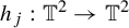 $h_j : \mathbb {T}^2\to \mathbb {T}^2$
be a smooth diffeomorphism that permutes equilibria by
$h_j : \mathbb {T}^2\to \mathbb {T}^2$
be a smooth diffeomorphism that permutes equilibria by
 $$ \begin{align*} h_j (s_i) := s_{i + j - 1 \mod k+1}. \end{align*} $$
For notational convenience, take $h_1$
to be the identity map. Write
$h_1$
to be the identity map. Write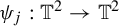 $\psi _j: \mathbb {T}^2 \to \mathbb {T}^2$
for maps
$\psi _j: \mathbb {T}^2 \to \mathbb {T}^2$
for maps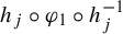 $h_j \circ \varphi _1 \circ h_j^{-1}$
. The maps
$h_j \circ \varphi _1 \circ h_j^{-1}$
. The maps $\psi _j$
,
$\psi _j$
, $1 \le j \le k$
will then be conjugate to each other by a smooth conjugacy. We find that
$1 \le j \le k$
will then be conjugate to each other by a smooth conjugacy. We find that $s_i$
is the unique attracting fixed point for
$s_i$
is the unique attracting fixed point for $\psi _{i}$
with open and dense basin
$\psi _{i}$
with open and dense basin $W^s (s_i)$
. Note also that the spectrum of
$W^s (s_i)$
. Note also that the spectrum of $D\psi _i (s_{i+j \mod k+1})$
is equal to the spectrum of
$D\psi _i (s_{i+j \mod k+1})$
is equal to the spectrum of $D\psi _1 (s_j)$
.
$D\psi _1 (s_j)$
.
As before, let E be an expanding map defined on $\mathbb {T}$
by
$\mathbb {T}$
by $E (x) := L x \pmod 1$
, where
$E (x) := L x \pmod 1$
, where $L>1$
is a large enough natural number ensuring that E has k fixed points
$L>1$
is a large enough natural number ensuring that E has k fixed points $q_1,\ldots , q_k$
. Let
$q_1,\ldots , q_k$
. Let $J_1,\ldots , J_k$
be disjoint open intervals in
$J_1,\ldots , J_k$
be disjoint open intervals in $\mathbb {T}$
, with
$\mathbb {T}$
, with $q_i \in J_i$
. Let
$q_i \in J_i$
. Let $t: \mathbb {T}\to [0,1]$
be a smooth function that is positive on
$t: \mathbb {T}\to [0,1]$
be a smooth function that is positive on $\bigcup _{i=1}^k J_i$
, vanishes outside
$\bigcup _{i=1}^k J_i$
, vanishes outside $\bigcup _{i=1}^k J_i$
, and satisfies
$\bigcup _{i=1}^k J_i$
, and satisfies $t(q_i) = 1$
. Finally, for a parameter
$t(q_i) = 1$
. Finally, for a parameter $u \in \mathbb {T}$
, take
$u \in \mathbb {T}$
, take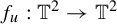 $f_u: \mathbb {T}^2 \to \mathbb {T}^2$
to be a diffeomorphism on
$f_u: \mathbb {T}^2 \to \mathbb {T}^2$
to be a diffeomorphism on $\mathbb {T}^2$
with the following properties:
$\mathbb {T}^2$
with the following properties:
-
(1) for
$u \in J_i$
and
$1 \le j \le k$
,
$$ \begin{align*}f_u := h_j \circ \varphi_{t(u)} \circ h_j^{-1};\end{align*} $$
-
(2) for each
$i=1,\ldots ,k$
,
$$ \begin{align*}\int_{\mathbb{T}} \log \|Df_u(s_i)\| \,du<0. \end{align*} $$





Item (2) can be achieved by choosing the flow $\varphi _t$
so that the eigenvalues of
$\varphi _t$
so that the eigenvalues of $D\psi _{i} (s_i)$
(which equal those at
$D\psi _{i} (s_i)$
(which equal those at $D\psi _1 (s_1)$
) are strongly contracting relative to the eigenvalues at the other equilibria. Observe that
$D\psi _1 (s_1)$
) are strongly contracting relative to the eigenvalues at the other equilibria. Observe that $f_u$
is a diffeomorphism that depends smoothly on u. For u outside
$f_u$
is a diffeomorphism that depends smoothly on u. For u outside $\bigcup _{i=1}^k J_i$
,
$\bigcup _{i=1}^k J_i$
, $f_u$
is the identity map. For each
$f_u$
is the identity map. For each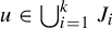 $u \in \bigcup _{i=1}^k J_i$
,
$u \in \bigcup _{i=1}^k J_i$
,
 $$ \begin{align*} \Omega (f_u) &= \{s_1,\ldots,s_{k}\}. \end{align*} $$
For comparison and inspiration for further constructions, we refer to [Reference Nozdrinova and Pochinka29].
Define the skew product F on $\mathbb {T}\times \mathbb {T}^2$
by
$\mathbb {T}\times \mathbb {T}^2$
by
 $$ \begin{align*} F(u,x) := (E(u),f_u(x)). \end{align*} $$
Theorem 2.4. The mapping F has k metric attractors $\mathbb {T}\times \{s_i\}$
,
$\mathbb {T}\times \{s_i\}$
, $i=1,\ldots ,k$
, whose basins are dense in
$i=1,\ldots ,k$
, whose basins are dense in $\mathbb {T}\times \mathbb {T}^2$
and mutually intermingled. The union
$\mathbb {T}\times \mathbb {T}^2$
and mutually intermingled. The union $\mathbb {T} \times \{s_1,\ldots ,s_{k}\}$
is the likely limit set.
$\mathbb {T} \times \{s_1,\ldots ,s_{k}\}$
is the likely limit set.
Proof. By item (2) above, the measures $\unicode{x3bb} \times \delta _{s_i}$
,
$\unicode{x3bb} \times \delta _{s_i}$
, $i=1,\ldots ,k$
, are invariant measures for F supported on
$i=1,\ldots ,k$
, are invariant measures for F supported on $\Lambda _i:= \mathbb {T}\times \{s_i\}$
,
$\Lambda _i:= \mathbb {T}\times \{s_i\}$
, $i=1,\ldots ,k$
whose fiber Lyapunov exponents are negative. In particular, by Pesin theory, see also the proof of Theorem 2.3, each
$i=1,\ldots ,k$
whose fiber Lyapunov exponents are negative. In particular, by Pesin theory, see also the proof of Theorem 2.3, each $\Lambda _i$
is a metric attractor of F. To prove that their basins are intermingled, suppose that
$\Lambda _i$
is a metric attractor of F. To prove that their basins are intermingled, suppose that $U\subset \mathbb {T}\times S$
is an open set. Choose a natural number N such that
$U\subset \mathbb {T}\times S$
is an open set. Choose a natural number N such that
 $$ \begin{align} F^N(U)\cap(\{q_i\}\times W^s(s_i))\neq \emptyset. \end{align} $$
Any point in the intersection (2.15) tends to $\Lambda _i$
under the iteration of F. The rest proceeds as in the proof of Theorem 2.3.
$\Lambda _i$
under the iteration of F. The rest proceeds as in the proof of Theorem 2.3.
2.2.2 Iterated function systems
Reference [Reference Gharaei and Homburg15] contains elementary constructions of skew products of interval diffeomorphisms over shifts, arising from iterated function systems, admitting metric attractors with intermingled basins. Here, we indicate analogous constructions for surface diffeomorphisms with more attractors.
Consider the iterated function system generated by $\psi _i$
,
$\psi _i$
, $1\le i\le k$
(defined in §2.2.1), and using equal probability
$1\le i\le k$
(defined in §2.2.1), and using equal probability $1/k$
for all of them. Assume that for all j between
$1/k$
for all of them. Assume that for all j between $1$
and k,
$1$
and k,
 $$ \begin{align} \frac{1}{k} \sum_{i=1}^{k} \ln \| D\psi_i (s_j)\| &< 0. \end{align} $$
Define  by
by
 $$ \begin{align} F(\omega,x) &:= (\sigma \omega , \varphi_{\omega_0} (x)). \end{align} $$
On $\Sigma _{k}$
, we take Bernoulli measure
$\Sigma _{k}$
, we take Bernoulli measure $\nu $
corresponding to equal probabilities for the symbols. The inequality (2.16) means that the fiber Lyapunov exponents at
$\nu $
corresponding to equal probabilities for the symbols. The inequality (2.16) means that the fiber Lyapunov exponents at $s_j$
, for any
$s_j$
, for any $1 \le j \le k$
, are negative. As in Theorem 2.4, we get the following result.
$1 \le j \le k$
, are negative. As in Theorem 2.4, we get the following result.
Theorem 2.5. Consider the skew product system F from (2.17) on $\Sigma _{k} \times \mathbb {T}^2$
. Take the product of Bernoulli measure
$\Sigma _{k} \times \mathbb {T}^2$
. Take the product of Bernoulli measure $\nu $
and Lebesgue measure
$\nu $
and Lebesgue measure $\unicode{x3bb} $
on
$\unicode{x3bb} $
on $\mathbb {T}^2$
as a reference measure. The sets
$\mathbb {T}^2$
as a reference measure. The sets $\Sigma _{k} \times \{s_i\}$
,
$\Sigma _{k} \times \{s_i\}$
, $1 \le i \le k$
are minimal metric attractors with intermingled basins. The union
$1 \le i \le k$
are minimal metric attractors with intermingled basins. The union $\Sigma _{k} \times \{s_1,\ldots ,s_{k}\}$
is the likely limit set.
$\Sigma _{k} \times \{s_1,\ldots ,s_{k}\}$
is the likely limit set.
2.2.3 Skew product systems over minimal torus diffeomorphisms
We provide a construction using a skew product system over minimal torus diffeomorphisms, motivated by [Reference Fayad13, Reference Melbourne and Windsor27, Reference Windsor34]. Let g be a conservative minimal $C^\infty $
diffeomorphism on
$C^\infty $
diffeomorphism on $T^2$
with two ergodic measures
$T^2$
with two ergodic measures $\mu _{\pm 1}$
each of which are absolutely continuous with respect to Lebesgue measure. Such a diffeomorphism can be built using the Anosov–Katok method from [Reference Anosov and Katok2] (see [Reference Melbourne and Windsor27, Reference Windsor34] for details). Put
$\mu _{\pm 1}$
each of which are absolutely continuous with respect to Lebesgue measure. Such a diffeomorphism can be built using the Anosov–Katok method from [Reference Anosov and Katok2] (see [Reference Melbourne and Windsor27, Reference Windsor34] for details). Put
 $$ \begin{align*} \Phi := \bigg\{\varphi:\mathbb{T}^2\to\mathbb{R}; \int_{\mathbb{T}^2} \varphi\, d\mu_{-1}<0<\int_{\mathbb{T}^2} \varphi\, d\mu_1\bigg\}. \end{align*} $$
It is not difficult to see that $\Phi $
is non-empty.
$\Phi $
is non-empty.
Lemma 2.6. For any $\varphi \in \Phi $
, there is a constant
$\varphi \in \Phi $
, there is a constant $c\in (0,1)$
such that the mapping
$c\in (0,1)$
such that the mapping  defined by
 $$ \begin{align*} H_c(x,t) := (g(x),\varphi(x) + c + t \pmod 1) \end{align*} $$
is minimal.
Proof. First, note that
 $$ \begin{align} H^n_c (x , t)=(g^n(x), \varphi^n (x) + n c + t \pmod 1 ), \end{align} $$
where by slight abuse of notation, we have written
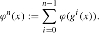 $$ \begin{align*} \varphi^n (x) := \sum_{i=0}^{n-1} \varphi (g^i(x)). \end{align*} $$
Let $\{V_k\}_{k\in \mathbb {N}}$
be an open basis of the topology on
$\{V_k\}_{k\in \mathbb {N}}$
be an open basis of the topology on $\mathbb {T}^2$
and
$\mathbb {T}^2$
and $x\in \mathbb {T}^2$
an arbitrary point. For any
$x\in \mathbb {T}^2$
an arbitrary point. For any $k\in \mathbb {N}$
, choose a sequence
$k\in \mathbb {N}$
, choose a sequence $\{n_i^{(k)}\}$
of natural numbers such that
$\{n_i^{(k)}\}$
of natural numbers such that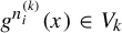 $g^{n_i^{(k)}}(x)\in V_k$
. Now, consider the mapping
$g^{n_i^{(k)}}(x)\in V_k$
. Now, consider the mapping $\Theta _{(x,k)}$
from
$\Theta _{(x,k)}$
from $[0,1]$
to the set of all closed subsets of
$[0,1]$
to the set of all closed subsets of $[0,1]$
(endowed with the Hausdorff distance) defined by
$[0,1]$
(endowed with the Hausdorff distance) defined by
 $$ \begin{align*} \Theta_{(x,k)}(c) := \text{Cl}\big(\big\{\varphi^{n_i^{(k)}}(x)+n_i^{(k)} c \pmod 1 \big\}_{i=0}^\infty\big). \end{align*} $$
Claim 1. The mapping $\Theta _{(x,k)}$
is lower semi-continuous.
$\Theta _{(x,k)}$
is lower semi-continuous.
Proof. For any given $\varepsilon>0$
, choose
$\varepsilon>0$
, choose $i_0\in \mathbb {N}$
such that
$i_0\in \mathbb {N}$
such that
 $$ \begin{align*} \text{Cl}\big(\big\{\varphi^{n_i^{(k)}}(x)+n_i^{(k)} c \pmod 1\big\}_{i=0}^\infty \big) \subseteq U_{\varepsilon/2} \big( \big\{\varphi^{n_i^{(k)}}(x)+n_i^{(k)} c \pmod 1\big\}_{i=0}^{i_0}\big). \end{align*} $$
Here, $U_{\varepsilon /2}(\cdot )$
stands for the open
$U_{\varepsilon /2}(\cdot )$
stands for the open $\varepsilon /2$
-neighborhood of the given closed set. Now, if
$\varepsilon /2$
-neighborhood of the given closed set. Now, if $\tilde {c}$
is sufficiently close to c, then
$\tilde {c}$
is sufficiently close to c, then
 $$ \begin{align*} \begin{aligned} U_\varepsilon\big(\text{Cl}\big( \big\{\varphi^{n_i^{(k)}}(x)+n_i^{(k)} \tilde{c} \pmod 1\big\}_{i=0}^\infty\big)\big) \supseteq & ~U_\varepsilon\big(\big\{\varphi^{n_i^{(k)}}(x)+n_i^{(k)} \tilde{c} \pmod 1\big\}_{i=0}^{i_0}\big)\\ \supseteq &~ U_{\varepsilon/2}\big(\big\{\varphi^{n_i^{(k)}}(x)+n_i^{(k)} c~(\text{mod}\,1)\big\}_{i=0}^{i_0}\big) \\ \supseteq & ~ \text{Cl}\big(\big\{\varphi^{n_i^{(k)}}(x)+n_i^{(k)} c \pmod 1\big\}_{i=0}^\infty\big). \end{aligned}\\[-34pt] \end{align*} $$
Let $\mathcal {R}_{(x,k)}$
be the set of continuity points of
$\mathcal {R}_{(x,k)}$
be the set of continuity points of $\Theta _{(x,k)}$
, which is known to be a residual set, and put
$\Theta _{(x,k)}$
, which is known to be a residual set, and put $\mathcal {R}_x=\bigcap _k \mathcal {R}_{(x,k)}$
, a residual set again. We prove that for any
$\mathcal {R}_x=\bigcap _k \mathcal {R}_{(x,k)}$
, a residual set again. We prove that for any $c\in \mathcal {R}_x$
,
$c\in \mathcal {R}_x$
, $\{H^n_c(x,t)\}_{n\in \mathbb {N}}$
is dense in
$\{H^n_c(x,t)\}_{n\in \mathbb {N}}$
is dense in $\mathbb {T}^2\times \mathbb {T}$
. To prove it, let
$\mathbb {T}^2\times \mathbb {T}$
. To prove it, let $U\times I$
be an arbitrary open set in
$U\times I$
be an arbitrary open set in $\mathbb {T}^2\times \mathbb {T}$
and choose k such that
$\mathbb {T}^2\times \mathbb {T}$
and choose k such that $V_k\subset U$
. Suppose by contradiction,
$V_k\subset U$
. Suppose by contradiction,
 $$ \begin{align} H_c^{n_i^{(k)}}(x,t)\not\in U\times I\quad \text{for any}~ i. \end{align} $$
However, recall (2.18),
 $$ \begin{align} H_c^{n_i^{(k)}}(x,t)=(g^{n_i^{(k)}}(x),\varphi^{n_i^{(k)}} (x)+n_i^{(k)}c+t \pmod 1 ). \end{align} $$
As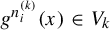 $g^{n_i^{(k)}}(x)\in V_k$
, (2.19) implies that
$g^{n_i^{(k)}}(x)\in V_k$
, (2.19) implies that $\varphi ^{n_i^{(k)}} (x)+n_i^{(k)}c+t \pmod 1\not \in I$
for any i. That is,
$\varphi ^{n_i^{(k)}} (x)+n_i^{(k)}c+t \pmod 1\not \in I$
for any i. That is, $\Theta _{(x,k)}(c)\cap I-t = \emptyset $
. However, (2.20) makes it clear that there are arbitrarily small
$\Theta _{(x,k)}(c)\cap I-t = \emptyset $
. However, (2.20) makes it clear that there are arbitrarily small $\delta>0$
so that
$\delta>0$
so that
 $$ \begin{align*} \Theta_{(x,k)}(c+\delta) \cap I-t \neq \emptyset. \end{align*} $$
This contradicts the fact that c is a continuity point of $\Theta _{(x,k)}$
.
$\Theta _{(x,k)}$
.
Having established the existence of a point $(x,t)$
with dense positive orbit, proving minimality follows from a standard argument using (2.18) and minimality of g. Namely, for any
$(x,t)$
with dense positive orbit, proving minimality follows from a standard argument using (2.18) and minimality of g. Namely, for any $\varepsilon>0$
, there is
$\varepsilon>0$
, there is $N_0$
so that
$N_0$
so that $\{(x,t), H_c(x,t),\ldots ,H^{N_0}_c (x,t)\}$
is
$\{(x,t), H_c(x,t),\ldots ,H^{N_0}_c (x,t)\}$
is $\varepsilon $
-dense in
$\varepsilon $
-dense in $\mathbb {T}^2\times \mathbb {T}$
. By (2.18), the same is true for any point from
$\mathbb {T}^2\times \mathbb {T}$
. By (2.18), the same is true for any point from $\{x\}\times \mathbb {T}$
replacing
$\{x\}\times \mathbb {T}$
replacing $(x,t)$
. For an arbitrary point
$(x,t)$
. For an arbitrary point $(y,s) \in \mathbb {T}^2 \times \mathbb {T}$
, since g is minimal, its positive orbit accumulates on a point
$(y,s) \in \mathbb {T}^2 \times \mathbb {T}$
, since g is minimal, its positive orbit accumulates on a point $(x,u)$
. It is therefore
$(x,u)$
. It is therefore $\varepsilon $
-dense. Since
$\varepsilon $
-dense. Since $\varepsilon $
is arbitrary,
$\varepsilon $
is arbitrary, $\{H^n_c (y,u)\}_{n\in \mathbb {N}}$
is dense for any
$\{H^n_c (y,u)\}_{n\in \mathbb {N}}$
is dense for any $(y,s) \in \mathbb {T}^2\times \mathbb {T}$
.
$(y,s) \in \mathbb {T}^2\times \mathbb {T}$
.
Let F be a north pole ( $p_N$
)/south pole (
$p_N$
)/south pole ( $p_S$
) diffeomorphism on
$p_S$
) diffeomorphism on $\mathbb {T}$
and consider its suspension flow defined by
$\mathbb {T}$
and consider its suspension flow defined by $F_s(y,t)=(y,t+s)$
on the suspended manifold M given by
$F_s(y,t)=(y,t+s)$
on the suspended manifold M given by $(y,t+1)\sim (F(y),t)$
(see for instance [Reference Palis and de Melo30, Ch. 3, Proposition 3.7] and [Reference Viana and Oliveira33, §3.4.1]). The flow
$(y,t+1)\sim (F(y),t)$
(see for instance [Reference Palis and de Melo30, Ch. 3, Proposition 3.7] and [Reference Viana and Oliveira33, §3.4.1]). The flow $F_s$
has invariant sets
$F_s$
has invariant sets
 $$ \begin{align*} \Lambda_S:= \{p_S\}\times \mathbb{T}, \quad \Lambda_N:= \{p_N\}\times \mathbb{T}. \end{align*} $$
Choose $\varphi \in \Phi $
and a constant c such that the mapping
$\varphi \in \Phi $
and a constant c such that the mapping $H_c$
defined in Lemma 2.6 is minimal. For simplicity, denote
$H_c$
defined in Lemma 2.6 is minimal. For simplicity, denote $\varphi +c$
by
$\varphi +c$
by $\varphi $
again. Define
$\varphi $
again. Define  by
by
 $$ \begin{align} H(x,(y,t)):=(g(x), F_{\varphi(x)}(y,t)). \end{align} $$
Theorem 2.7. The mapping H defining by (2.21) has two metric attractors $\mathbb {T}^2\times \Lambda _S$
and
$\mathbb {T}^2\times \Lambda _S$
and $\mathbb {T}^2\times \Lambda _N$
whose basins are intermingled.
$\mathbb {T}^2\times \Lambda _N$
whose basins are intermingled.
Proof. Note that
 $$ \begin{align} H^n(x,(y,t)) &= (g^n(x), F_{\varphi^n(x)}(y,t)) \nonumber \\ &=(g^n(x), F^{[t+\varphi^n(x)]}(y), t+\varphi^n(x) \pmod 1), \end{align} $$
where $[\cdot ]$
denotes the integer part and, as before,
$[\cdot ]$
denotes the integer part and, as before, $\varphi ^n(x)=\sum _{i=0}^{n-1} \varphi (g^i(x))$
.
$\varphi ^n(x)=\sum _{i=0}^{n-1} \varphi (g^i(x))$
.
In view of Lemma 2.6, $\mathbb {T}^2\times \Lambda _S$
and
$\mathbb {T}^2\times \Lambda _S$
and $\mathbb {T}^2\times \Lambda _N$
are metric attractors of H. We prove that the basins of attraction are intermingled. For this, let
$\mathbb {T}^2\times \Lambda _N$
are metric attractors of H. We prove that the basins of attraction are intermingled. For this, let $(x,(y,t))$
be an arbitrary point in
$(x,(y,t))$
be an arbitrary point in $\mathbb {T}^2\times M$
. Take
$\mathbb {T}^2\times M$
. Take $\tilde {x}$
close to x to be a generic point with respect to
$\tilde {x}$
close to x to be a generic point with respect to $\mu _1$
and
$\mu _1$
and $\tilde {y}\neq p_N$
close to y. It is not difficult to see that by (2.22),
$\tilde {y}\neq p_N$
close to y. It is not difficult to see that by (2.22),
 $$ \begin{align*} H^n(\tilde{x},(\tilde{y},t))\to \mathbb{T}^2\times \Lambda_S \end{align*} $$
as $n \to \infty $
. Likewise, take
$n \to \infty $
. Likewise, take $\hat {x}$
, a generic point with respect to
$\hat {x}$
, a generic point with respect to $\mu _{-1}$
, and
$\mu _{-1}$
, and $\hat {y}\neq p_S$
, sufficiently close to x and y, respectively. Then,
$\hat {y}\neq p_S$
, sufficiently close to x and y, respectively. Then,
 $$ \begin{align*} H^n(\hat{x},(\hat{y},t))\to \mathbb{T}^2\times \Lambda_N \end{align*} $$
as $n\to \infty $
.
$n\to \infty $
.
3 Flows of smooth vector fields
We construct similar examples for flows of smooth vector fields. Let us first remark that the definitions of metric attractor, likely limit set, and intermingled basin given in the introduction for continuous maps transfer to flows $x\mapsto \phi _t (x)$
generated by differential equations.
$x\mapsto \phi _t (x)$
generated by differential equations.
We will consider skew product systems over an ergodic volume preserving flow. To be concrete, let g be a smooth vector field that generates the suspension of a hyperbolic torus automorphism. The flow $\psi _t: M \to M$
of
$\psi _t: M \to M$
of
 $$ \begin{align} \dot{u} &= g(u) \end{align} $$
on $M := \mathbb {T}^3 = (\mathbb {R}/\mathbb {Z})^3$
preserves Lebesgue measure
$M := \mathbb {T}^3 = (\mathbb {R}/\mathbb {Z})^3$
preserves Lebesgue measure $\unicode{x3bb} $
and is ergodic. Consider the flow
$\unicode{x3bb} $
and is ergodic. Consider the flow $\varphi _t: N \to N$
of a Morse–Smale gradient differential equation
$\varphi _t: N \to N$
of a Morse–Smale gradient differential equation $\dot {x} = f(x) = -\text {grad}(h)$
on a compact manifold N as in (2.12) and (2.13). We will also write
$\dot {x} = f(x) = -\text {grad}(h)$
on a compact manifold N as in (2.12) and (2.13). We will also write $\varphi (t,x) = \varphi _t (x)$
. Take a skew product systems of the form
$\varphi (t,x) = \varphi _t (x)$
. Take a skew product systems of the form
 $$ \begin{align} \nonumber \dot{u} &= g(u), \\ \dot{x} &= \zeta(u,x) f(x), \end{align} $$
with $(u,x) \in M \times N$
and with
$(u,x) \in M \times N$
and with $\zeta : M \times N \to \mathbb {R}$
a smooth scalar function. Take volume on
$\zeta : M \times N \to \mathbb {R}$
a smooth scalar function. Take volume on $M\times N$
as a reference measure. Write
$M\times N$
as a reference measure. Write $\Phi _t(u,x)$
for the flow of (3.2).
$\Phi _t(u,x)$
for the flow of (3.2).
Example 3.1. A special case is where $\zeta (u,x) =\eta (u)$
depends only on u. Let
$\zeta (u,x) =\eta (u)$
depends only on u. Let $\eta : M \to \mathbb {R}$
be a smooth scalar function taking positive and negative values, and satisfying
$\eta : M \to \mathbb {R}$
be a smooth scalar function taking positive and negative values, and satisfying
 $$ \begin{align} \int_{M} \eta (u) \, d\unicode{x3bb}(u) &> 0. \end{align} $$
Consider
 $$ \begin{align} \begin{aligned} \dot{u} &= g(u), \\ \dot{x} &= \eta(u) f(x). \end{aligned} \end{align} $$
For different values of $\eta $
, the flow
$\eta $
, the flow $\varphi (t,x_0)$
of f is followed in different time directions. Observe that
$\varphi (t,x_0)$
of f is followed in different time directions. Observe that
 $$ \begin{align*} \Phi_t (u_0,x_0) = (\psi_t (u_0) , \varphi (\tau(t) , x_0)) \end{align*} $$
with
 $$ \begin{align*} \tau(t) = \int_0^t \eta(u(s)) \, ds. \end{align*} $$
By Birkhoff’s ergodic theorem, we find $\tau (t) \to \infty $
as
$\tau (t) \to \infty $
as $t \to \infty $
for almost all
$t \to \infty $
for almost all $u_0 \in M$
. Thus,
$u_0 \in M$
. Thus, $M \times \{p_S\}$
is a metric attractor and also the likely limit set.
$M \times \{p_S\}$
is a metric attractor and also the likely limit set.
Analogous to the choice of the function s in §2.2, take the smooth function $\zeta : M \times N \to \mathbb {R}$
with the following properties:
$\zeta : M \times N \to \mathbb {R}$
with the following properties:
-
(1) there are hyperbolic periodic orbits
$q_1, q_2$
for g for which
$$ \begin{align*} \zeta \vert_{\{q_1\} \times N}> 0, \quad \zeta \vert_{\{q_2\} \times N} <0; \end{align*} $$
-
(2) we have
$$ \begin{align*} \int_{M} \zeta (u,p_S) \, d\unicode{x3bb}(u)> 0, \quad \int_{M} \zeta (u,p_N) \, d\unicode{x3bb}(u) < 0. \end{align*} $$


Now,
 $$ \begin{align*} \lim_{t\to \infty} \frac{1}{t} \ln (\| D\varphi_{\tau(t)} (p_S) \|) \quad \text{with }\tau (t) = \int_0^t \zeta (u(s), p_S)\, ds, \end{align*} $$
is negative, which means as in §2.2 that the fiber Lyapunov exponents at $p_S$
are negative. Likewise, we have only negative fiber Lyapunov exponents at
$p_S$
are negative. Likewise, we have only negative fiber Lyapunov exponents at $p_N$
.
$p_N$
.
Theorem 3.2. Consider the differential equation (3.2) on $M \times N$
and suppose
$M \times N$
and suppose $\zeta $
satisfies properties (1) and (2) above. Take volume on
$\zeta $
satisfies properties (1) and (2) above. Take volume on $M \times N$
as a reference measure. Then,
$M \times N$
as a reference measure. Then, $M \times \{ p_N\} $
and
$M \times \{ p_N\} $
and $M \times \{p_S\}$
are metric attractors for the flow
$M \times \{p_S\}$
are metric attractors for the flow $\Phi _t$
of (3.2) with intermingled basins. The union
$\Phi _t$
of (3.2) with intermingled basins. The union $M \times \{ p_N,p_S\}$
is the likely limit set.
$M \times \{ p_N,p_S\}$
is the likely limit set.
Proof. Take a neighborhood U of $p_S$
and a smooth scalar function
$p_S$
and a smooth scalar function $\eta : M \to \mathbb {R}$
so that
$\eta : M \to \mathbb {R}$
so that
 $$ \begin{align} \eta (u) < \zeta (u,x), \quad u \in M, x \in U, \end{align} $$
and so that (3.3) holds. Let $z(t)$
be a solution to
$z(t)$
be a solution to $\dot {z} = f(z)$
contained in the basin of attraction of
$\dot {z} = f(z)$
contained in the basin of attraction of $p_S$
for the flow
$p_S$
for the flow $\varphi _t$
. Take a solution
$\varphi _t$
. Take a solution $(u(t) , x(t))$
to (3.4) with
$(u(t) , x(t))$
to (3.4) with $u(0) = u_0$
and
$u(0) = u_0$
and $x(0) = z (T)$
for some T. Write
$x(0) = z (T)$
for some T. Write $x(t) = z(\tau (t))$
, where
$x(t) = z(\tau (t))$
, where $\tau (0)=T$
.
$\tau (0)=T$
.
For almost all $u_0 \in M$
,
$u_0 \in M$
, $\lim _{t\to \infty } \tau (t) = \infty $
(see Example 3.1). For such
$\lim _{t\to \infty } \tau (t) = \infty $
(see Example 3.1). For such $u_0$
,
$u_0$
, $\tau (t)$
for
$\tau (t)$
for $t \ge 0$
has a minimum value. For a larger starting point
$t \ge 0$
has a minimum value. For a larger starting point $\tau (0) = T$
, the minimum value increases. Now, T large corresponds to an initial point close to
$\tau (0) = T$
, the minimum value increases. Now, T large corresponds to an initial point close to $p_S$
. So, for T large enough,
$p_S$
. So, for T large enough, $x(t)$
,
$x(t)$
, $t \ge 0$
, stays in a neighborhood of
$t \ge 0$
, stays in a neighborhood of $p_S$
and converges to
$p_S$
and converges to $p_S$
. This shows that for almost all
$p_S$
. This shows that for almost all $u \in M$
, there are local stable manifolds
$u \in M$
, there are local stable manifolds $\{u\} \times U_u$
of
$\{u\} \times U_u$
of $(u,p_S)$
. By (3.5), these manifolds are local stable manifolds of
$(u,p_S)$
. By (3.5), these manifolds are local stable manifolds of $(u,p_S)$
also for (3.2). Likewise, there are local stable manifolds
$(u,p_S)$
also for (3.2). Likewise, there are local stable manifolds $u \times V_u$
of
$u \times V_u$
of $(u,p_N)$
for which
$(u,p_N)$
for which $\Phi _t (u,z)$
,
$\Phi _t (u,z)$
, $z \in V_u$
, converges to
$z \in V_u$
, converges to $M \times \{p_N\}$
as
$M \times \{p_N\}$
as $t \to \infty $
. We conclude that
$t \to \infty $
. We conclude that $M \times \{p_N\}$
and
$M \times \{p_N\}$
and $M \times \{p_S\}$
are metric attractors.
$M \times \{p_S\}$
are metric attractors.
Write
 $$ \begin{align*} W^s (M\times \{p_S\}) := \bigcup_{u \in M} \{u\} \times U_u \end{align*} $$
for the union of local stable manifolds of $(u,p_S)$
and
$(u,p_S)$
and
 $$ \begin{align*} W^s (M\times \{p_N\}) := \bigcup_{u \in M} \{u\} \times V_u \end{align*} $$
for the union of local stable manifolds of $(u,p_N)$
. Now, take an open set
$(u,p_N)$
. Now, take an open set $U \subset M \times N$
. Since stable manifolds of periodic orbits of (3.1) lie dense in M, any open set will intersect the stable manifolds of
$U \subset M \times N$
. Since stable manifolds of periodic orbits of (3.1) lie dense in M, any open set will intersect the stable manifolds of $q_1$
and
$q_1$
and $q_2$
from property (1). This implies that for large enough t,
$q_2$
from property (1). This implies that for large enough t, $\Phi _t (U)$
intersects both
$\Phi _t (U)$
intersects both $W^s (M\times \{p_S\})$
and
$W^s (M\times \{p_S\})$
and $W^s (M\times \{p_N\})$
in sets of positive measure. The metric attractors
$W^s (M\times \{p_N\})$
in sets of positive measure. The metric attractors $M \times \{p_N\}$
and
$M \times \{p_N\}$
and $M \times \{p_S\}$
therefore have intermingled basins of attraction, where both basins lie dense in
$M \times \{p_S\}$
therefore have intermingled basins of attraction, where both basins lie dense in $M\times N$
.
$M\times N$
.
The proof that $M \times \{p_N,p_S\}$
is the likely limit set goes as in Theorem 2.3. We give a brief account. As in that proof, consider the set
$M \times \{p_N,p_S\}$
is the likely limit set goes as in Theorem 2.3. We give a brief account. As in that proof, consider the set $\Lambda \subset M\times B$
consisting of points whose
$\Lambda \subset M\times B$
consisting of points whose $\omega $
-limit sets are not contained in
$\omega $
-limit sets are not contained in $M \times \{p_N,p_S\}$
. Suppose
$M \times \{p_N,p_S\}$
. Suppose $\Lambda $
has positive volume. Then, by Fubini’s theorem, there is a slice
$\Lambda $
has positive volume. Then, by Fubini’s theorem, there is a slice $M \times \{y\}$
for some
$M \times \{y\}$
for some $y \in B$
that intersects
$y \in B$
that intersects $\Lambda $
in a set of positive volume. Take a Lebesgue density point
$\Lambda $
in a set of positive volume. Take a Lebesgue density point $(v,y)$
of
$(v,y)$
of $\Lambda \cap (M \times \{y\})$
. Consider the flow of a small ball
$\Lambda \cap (M \times \{y\})$
. Consider the flow of a small ball $\Sigma $
around
$\Sigma $
around $(v,y)$
in
$(v,y)$
in $M \times \{y\}$
. For high enough t,
$M \times \{y\}$
. For high enough t, $\Phi _t (\Sigma )$
will intersect the union of local stable manifolds of
$\Phi _t (\Sigma )$
will intersect the union of local stable manifolds of $(u,p_N)$
and the union of local stable manifolds of
$(u,p_N)$
and the union of local stable manifolds of $(u,p_S)$
. These intersections are of positive measure. Since the dynamics in the base is a suspension of a linear hyperbolic torus map, the proportion
$(u,p_S)$
. These intersections are of positive measure. Since the dynamics in the base is a suspension of a linear hyperbolic torus map, the proportion $\Lambda \cap \Sigma $
in
$\Lambda \cap \Sigma $
in $\Sigma $
remains unchanged under iteration. This gives a contradiction.
$\Sigma $
remains unchanged under iteration. This gives a contradiction.
Corollary 3.3. Consider the time-one map $\Phi _1$
on
$\Phi _1$
on $\mathbb {T}^2 \times N$
. Then,
$\mathbb {T}^2 \times N$
. Then, $\mathbb {T}^2 \times \{ p_N\}$
and
$\mathbb {T}^2 \times \{ p_N\}$
and $\mathbb {T}^2 \times \{p_S\}$
are metric attractors for
$\mathbb {T}^2 \times \{p_S\}$
are metric attractors for $\Phi _1$
with intermingled basins.
$\Phi _1$
with intermingled basins.
Proof. Take $(u_0,0) \in \mathbb {T}^2 \times \mathbb {T}$
. The orbit
$(u_0,0) \in \mathbb {T}^2 \times \mathbb {T}$
. The orbit $\Phi _t (u_0,0, x_0)$
converges to
$\Phi _t (u_0,0, x_0)$
converges to $M \times \{p_S\}$
if and only if the sequence
$M \times \{p_S\}$
if and only if the sequence $(u_n,x_n) = \Phi _n (u_0,x_0)$
,
$(u_n,x_n) = \Phi _n (u_0,x_0)$
, $n \in \mathbb {N}$
, converges to
$n \in \mathbb {N}$
, converges to $\mathbb {T}^2 \times \{p_S\}$
.
$\mathbb {T}^2 \times \{p_S\}$
.
4 Intermingled basins of two thick attractors
This section contains a construction of a skew product system, arising from an iterated function system, possessing a pair of thick attractors with intermingled basins. We start with the construction of an iterated function system with both a thick attractor and a thick repeller, after which a random walk on orbits is introduced. We continue with sketching alternative constructions, leading to skew product systems with several thick metric attractors and mutually intermingled basins. We will restrict to skew product systems over symbolic dynamics, and will not discuss extensions to smooth maps.
4.1 Iterated function system with a thick attractor/thick repeller pair
In building a model, we start with the introduction of an iterated function system on the unit interval $[0,1]$
generated by two diffeomorphisms
$[0,1]$
generated by two diffeomorphisms $f_0,f_1$
.
$f_0,f_1$
.
The graphs of $f_0$
and
$f_0$
and $f_1$
are sketched in Figure 1. Both maps fix the end points
$f_1$
are sketched in Figure 1. Both maps fix the end points $0$
and
$0$
and $1$
. For points
$1$
. For points $0<l<r<1$
, we have
$0<l<r<1$
, we have
 $$ \begin{align*} f_1 (l) &= l, \quad f_1(x)> x \quad\textrm{ for } x \in (0,l), \\ f_1 (r) &= r, \quad f_1(x) > x \quad\textrm{ for } x \in (r,1). \end{align*} $$
We further have
 $$ \begin{align*} f_0(x) < x \quad\textrm{ for } x \in (0,1), \quad f_1(x) < x \quad\textrm{ for } x \in (l,r). \end{align*} $$
The interval $I_l = [0,l]$
is mapped into itself by
$I_l = [0,l]$
is mapped into itself by $f_0$
and
$f_0$
and $f_1$
. The interval
$f_1$
. The interval $I_r = [r,1]$
is mapped into itself by
$I_r = [r,1]$
is mapped into itself by $f_0^{-1}$
and
$f_0^{-1}$
and $f_1^{-1}$
. We take conditions on derivatives at
$f_1^{-1}$
. We take conditions on derivatives at $0$
and
$0$
and $1$
, namely
$1$
, namely
 $$ \begin{align*} f_0'(0)f_1'(0)> 1, \quad (f_0^{-1})'(1)(f_1^{-1})'(1) > 1, \end{align*} $$
and generic conditions on second-order derivatives, see [Reference Ilyashenko22, §3.1] or [Reference Gharaei and Homburg15, Proposition 2.1].
We consider an iterated function system generated by diffeomorphisms $f_0$
and
$f_0$
and $f_1$
on
$f_1$
on $[0,1]$
with graphs as depicted. There is an invariant interval
$[0,1]$
with graphs as depicted. There is an invariant interval $I_l = [0,l]$
. For the inverse maps
$I_l = [0,l]$
. For the inverse maps $f_0^{-1}$
and
$f_0^{-1}$
and $f_1^{-1}$
, the interval
$f_1^{-1}$
, the interval $I_r = [r,1]$
is invariant.
$I_r = [r,1]$
is invariant.
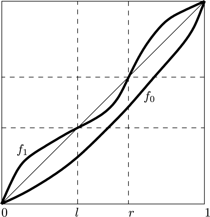
The iterated function system generated by $f_0$
and
$f_0$
and $f_1$
has a representation as a skew product system
$f_1$
has a representation as a skew product system  given by
 $$ \begin{align*} F(\omega , x) &:= (\sigma \omega , f_{\omega_0} (x) ). \end{align*} $$
This defines a homeomorphism on $ \Sigma _2 \times [0,1]$
. Denote iterates of F by
$ \Sigma _2 \times [0,1]$
. Denote iterates of F by
 $$ \begin{align*} F^n (\omega,x) = (\sigma^n , f^n_\omega (x)). \end{align*} $$
On $\Sigma _2$
, we take Bernoulli measure
$\Sigma _2$
, we take Bernoulli measure $\nu _{1/2}$
. By [Reference Ilyashenko21], the map F restricted to
$\nu _{1/2}$
. By [Reference Ilyashenko21], the map F restricted to $\Sigma _2 \times I_l$
admits a thick metric attractor
$\Sigma _2 \times I_l$
admits a thick metric attractor
 $$ \begin{align*} \Lambda_l := \bigcap_{n=0}^{\infty} F^n ( \Sigma_2 \times I_l ) \end{align*} $$
with $\nu _{1/2}\times \unicode{x3bb} (\Lambda _l)> 0$
. The attractor is characterized by
$\nu _{1/2}\times \unicode{x3bb} (\Lambda _l)> 0$
. The attractor is characterized by
 $$ \begin{align*} \Lambda_l &= \{(\omega , [0, X_l (\omega)] ); \omega \in \Sigma_2 \} \end{align*} $$
for an invariant measurable function $X_l : \Sigma _2 \to [0,l]$
with
$X_l : \Sigma _2 \to [0,l]$
with $X_l> 0$
almost everywhere. The values
$X_l> 0$
almost everywhere. The values $X_l(\omega )$
are obtained from a pullback construction
$X_l(\omega )$
are obtained from a pullback construction
 $$ \begin{align} X_l(\omega) &:= \lim_{n\to\infty} f^n_{\sigma^{-n} \omega} (l), \end{align} $$
where $f^n_{\sigma ^{-n} \omega } (l)$
is a monotone decreasing sequence. For any
$f^n_{\sigma ^{-n} \omega } (l)$
is a monotone decreasing sequence. For any $(\omega ,x) \in \Lambda _l$
with
$(\omega ,x) \in \Lambda _l$
with $0 < x < X_l(\omega )$
and any neighborhood U of
$0 < x < X_l(\omega )$
and any neighborhood U of $(\omega ,x)$
, there is a point
$(\omega ,x)$
, there is a point $(\omega ', X_l (\omega ')) \in U$
.
$(\omega ', X_l (\omega ')) \in U$
.
The skew product F likewise admits a thick metric repeller
 $$ \begin{align*} \Lambda_r := \bigcap_{i=0}^{\infty} F^{-i} ( \Sigma_2 \times I_r ) \end{align*} $$
in $\Omega ^+ \times I_r$
. That is,
$\Omega ^+ \times I_r$
. That is, $\nu _{1/2} \times \unicode{x3bb} (\Lambda _r)>0$
and
$\nu _{1/2} \times \unicode{x3bb} (\Lambda _r)>0$
and $\Lambda _r$
is a thick attractor for
$\Lambda _r$
is a thick attractor for $F^{-1}$
. The argument of [Reference Ilyashenko21, Remark 1] and (4.1) shows that every open ball
$F^{-1}$
. The argument of [Reference Ilyashenko21, Remark 1] and (4.1) shows that every open ball $U \subset \Sigma _2 \times [0,1]$
has non-empty intersection with the complement of
$U \subset \Sigma _2 \times [0,1]$
has non-empty intersection with the complement of $\Lambda _l \cup \Lambda _r$
.
$\Lambda _l \cup \Lambda _r$
.
4.2 Thick metric attractors with intermingled basins
The next step is to define a random walk on orbits of F. As before, with $\Omega := \{-1,+1\}^{\mathbb {Z}}$
, define
$\Omega := \{-1,+1\}^{\mathbb {Z}}$
, define  by
by
 $$ \begin{align*} G(\eta,\omega,x) &:= (\sigma \eta , F^{\eta_0} (\omega,x) ). \end{align*} $$
Take a continuous function $p: [0,1] \to (0,1)$
with
$p: [0,1] \to (0,1)$
with
 $$ \begin{align*} p(x) = p_l> 1/2\quad \text{ for } x \in I_l, \quad p(x) = p_r < 1/2\quad \text{ for } x \in I_r. \end{align*} $$
Let $\zeta _{\omega ,x}$
be the measure on
$\zeta _{\omega ,x}$
be the measure on $\Omega $
which is defined on cylinders by
$\Omega $
which is defined on cylinders by
 $$ \begin{align*} \zeta_{\omega,x} ([a_0\cdots a_k]) &:= \prod_{i=0}^k p_{a_i} (f^{S_i (a)}_\omega (x)), \end{align*} $$
where, as before, $p_{-1} (x) := 1 - p (x)$
and
$p_{-1} (x) := 1 - p (x)$
and $p_{1} (x) := p(x)$
and
$p_{1} (x) := p(x)$
and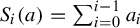 $S_i(a) = \sum _{i=0}^{i-1} a_i$
. Define the measure
$S_i(a) = \sum _{i=0}^{i-1} a_i$
. Define the measure $\mu $
on
$\mu $
on $\Omega \times \Sigma _2 \times [0,1]$
by
$\Omega \times \Sigma _2 \times [0,1]$
by

where $A_{(\omega ,x)} = A \cap (\Omega ^+ \times \{(\omega ,x)\})$
. Iterates of G are of the form
$A_{(\omega ,x)} = A \cap (\Omega ^+ \times \{(\omega ,x)\})$
. Iterates of G are of the form
 $$ \begin{align*} G^n (\eta,\omega,x) &= (\sigma^n \eta, \sigma^{S_n(\eta)} \omega, f^{S_n (\eta)}_\omega (x) ). \end{align*} $$
As in the proof of Theorem 2.2, we find that for $\mu $
-almost all
$\mu $
-almost all $(\eta ,x)$
,
$(\eta ,x)$
, $S_n(\eta )$
goes to
$S_n(\eta )$
goes to $\infty $
or
$\infty $
or $-\infty $
as
$-\infty $
as $n\to \infty $
.
$n\to \infty $
.
With  given by
 $$ \begin{align*} \chi (\eta,\omega) := (\sigma \eta, \sigma^{\eta_0} \omega), \end{align*} $$
we can consider G as a skew product of interval diffeomorphisms over $\chi $
. Namely,
$\chi $
. Namely,
 $$ \begin{align*} G(\eta,\omega,x) = \begin{cases} ( \chi (\eta,\omega), f_0(x)), & (\eta_0,\omega_0) = (+,0), \\ (\chi (\eta,\omega),f_1(x)), & (\eta_0,\omega_0) = (+,1),\\ (\chi (\eta,\omega),f_0^{-1}(x)), & (\eta_0,\omega_{-1}) = (-,0), \\ (\chi (\eta,\omega),f_1^{-1}(x)), & (\eta_0,\omega_{-1}) = (-,1). \end{cases} \end{align*} $$
For (positive) orbits contained in $\Omega \times \Sigma _2 \times I_l$
, the measure we consider on
$\Omega \times \Sigma _2 \times I_l$
, the measure we consider on $\Omega $
is
$\Omega $
is $\nu _{p_l}$
. For such orbits, the following lemma becomes useful.
$\nu _{p_l}$
. For such orbits, the following lemma becomes useful.
Lemma 4.1. The measure $P := \nu _{p_l} \times \nu _{1/2}$
is an invariant ergodic measure for
$P := \nu _{p_l} \times \nu _{1/2}$
is an invariant ergodic measure for $\chi $
.
$\chi $
.
Proof. Invariance of P is clear and so we only have to prove ergodicity. In the same way that the shift on $\Sigma _2$
endowed with Bernoulli measure
$\Sigma _2$
endowed with Bernoulli measure $\nu _{p}$
is measurably isomorphic to the two-dimensional baker’s map
$\nu _{p}$
is measurably isomorphic to the two-dimensional baker’s map $B_p$
(from (2.2)), one has that
$B_p$
(from (2.2)), one has that $\chi $
, endowed with P, is measurably isomorphic to
$\chi $
, endowed with P, is measurably isomorphic to  given by
 $$ \begin{align*} J(x,y,u,v) := \begin{cases} (B_p(x,y) , B_{1/2} (u,v)), & 0 \le x < p, \\ (B_p(x,y) , B_{1/2}^{-1} (u,v)), & p \le x \le 1, \end{cases} \end{align*} $$
and endowed with Lebesgue measure. Lebesgue measure is indeed invariant for J. For Lebesgue almost all points, there are local stable and local unstable manifolds. Namely, for Lebesgue almost all $x_0$
,
$x_0$
, $W^s := \{ x = x_0, 0\le y,u,v < 1\}$
has the property that
$W^s := \{ x = x_0, 0\le y,u,v < 1\}$
has the property that $G^n (x_0,y,u,v) - G^n(x_0,y',u',v')$
goes to zero as
$G^n (x_0,y,u,v) - G^n(x_0,y',u',v')$
goes to zero as $n\to \infty $
. Similar for
$n\to \infty $
. Similar for $W^u := \{ y = y_0, u=u_0, v=v_0, 0\le x < 1\}$
and iterates under
$W^u := \{ y = y_0, u=u_0, v=v_0, 0\le x < 1\}$
and iterates under $G^{-n}$
. A standard Hopf argument (see [Reference Viana and Oliveira33, §4.2.6]) shows ergodicity, just as for hyperbolic diffeomorphisms. We note that [Reference Homburg and Kalle19, Theorem 3.2] treats a similar situation of piecewise linear maps.
$G^{-n}$
. A standard Hopf argument (see [Reference Viana and Oliveira33, §4.2.6]) shows ergodicity, just as for hyperbolic diffeomorphisms. We note that [Reference Homburg and Kalle19, Theorem 3.2] treats a similar situation of piecewise linear maps.
Theorem 4.2. Consider the skew product system F from (2.14) on $\Omega \times \Sigma _2 \times [0,1]$
. Take
$\Omega \times \Sigma _2 \times [0,1]$
. Take $\mu $
as a reference measure. The sets
$\mu $
as a reference measure. The sets $\Omega \times \Lambda _l$
and
$\Omega \times \Lambda _l$
and $\Omega \times \Lambda _r$
are thick metric attractors for G with intermingled basins. The union
$\Omega \times \Lambda _r$
are thick metric attractors for G with intermingled basins. The union $\Omega \times (\Lambda _l \cup \Lambda _r)$
is the likely limit set.
$\Omega \times (\Lambda _l \cup \Lambda _r)$
is the likely limit set.
Proof. The identity
 $$ \begin{align*} G (\eta , \omega, X_l (\omega)) = (\sigma \eta , \sigma^{\eta_0} \omega , X_l (\sigma^{\eta_0} \omega)) \end{align*} $$
implies that $\Omega \times \Lambda _l$
is invariant for G. The same is true for
$\Omega \times \Lambda _l$
is invariant for G. The same is true for $\Omega \times \Lambda _r$
. As in the proof of Theorem 2.2, we find that
$\Omega \times \Lambda _r$
. As in the proof of Theorem 2.2, we find that $\mu $
-almost all orbits converge to either
$\mu $
-almost all orbits converge to either $\Omega \times \Lambda _l$
or
$\Omega \times \Lambda _l$
or $\Omega \times \Lambda _r$
. It remains to show that these sets are thick metric attractors.
$\Omega \times \Lambda _r$
. It remains to show that these sets are thick metric attractors.
To show that $\Omega \times \Lambda _l$
is a thick metric attractor, we follow [Reference Ilyashenko21, Lemma 2]. Let us summarize this approach for the skew product system F on
$\Omega \times \Lambda _l$
is a thick metric attractor, we follow [Reference Ilyashenko21, Lemma 2]. Let us summarize this approach for the skew product system F on $\Sigma _2 \times I_l$
over the shift
$\Sigma _2 \times I_l$
over the shift $\sigma $
, and then discuss how to adapt it to the setting of a skew product over
$\sigma $
, and then discuss how to adapt it to the setting of a skew product over $\chi $
.
$\chi $
.
An invariant measure for F is called good if it is a weak limit of $({1}/{n}) \sum _{k=0}^{n-1} F^k_* (\nu _{1/2} \times \unicode{x3bb} )$
. Put
$({1}/{n}) \sum _{k=0}^{n-1} F^k_* (\nu _{1/2} \times \unicode{x3bb} )$
. Put
 $$ \begin{align*} A_{\min}:=\text{Cl}\bigg( \bigcup_{\mu\,\text{is a good measure}} \text{Supp}(\mu)\bigg). \end{align*} $$
Following the notation of [Reference Ilyashenko21], we call $A_{\min }$
the minimal attractor of F. By [Reference Gorodetskii and Ilyashenko16, Reference Ilyashenko20],
$A_{\min }$
the minimal attractor of F. By [Reference Gorodetskii and Ilyashenko16, Reference Ilyashenko20], $A_{\min }\subseteq \Lambda _r$
and furthermore, as shown in [Reference Ilyashenko21],
$A_{\min }\subseteq \Lambda _r$
and furthermore, as shown in [Reference Ilyashenko21],
 $$ \begin{align*} \nu_{1/2} (\{ \omega \in \Sigma_2; (\omega,X_l(\omega)) \in A_{\min}\} ) = 1, \end{align*} $$
after which the proof can be concluded by studying the properties of $X_l$
.
$X_l$
.
Now, we turn to the skew product G. Put
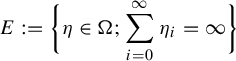 $$ \begin{align*} E := \bigg\{ \eta \in \Omega; \sum_{i=0}^{\infty} \eta_i = \infty\bigg\} \end{align*} $$
and note that $\nu _{p_l} (E)=1$
. For a point
$\nu _{p_l} (E)=1$
. For a point $p \in \Omega \times \Sigma _2\times [0,1]$
, write
$p \in \Omega \times \Sigma _2\times [0,1]$
, write $x(p)$
for the coordinate in
$x(p)$
for the coordinate in $[0,1]$
. For
$[0,1]$
. For $\eta \in E$
and
$\eta \in E$
and $\omega \in \Sigma _2$
, there exists
$\omega \in \Sigma _2$
, there exists $y := y(\eta ,\omega ) \in (X_l(\omega ),l)$
so that
$y := y(\eta ,\omega ) \in (X_l(\omega ),l)$
so that $x (G^n (\eta ,\omega ,u)) \le l$
for all
$x (G^n (\eta ,\omega ,u)) \le l$
for all $u \le y$
and
$u \le y$
and $n\ge 0$
. In fact,
$n\ge 0$
. In fact, $G^n (\eta ,\omega ,y)$
converges to the graph of
$G^n (\eta ,\omega ,y)$
converges to the graph of $X_l$
as
$X_l$
as $n\to \infty $
. The set
$n\to \infty $
. The set
 $$ \begin{align*} \mathcal{K} := \{ (\eta,\omega,u) \in \Omega\times \Sigma_2\times I_l; \eta \in E, X_l(\omega) < u < y(\eta,\omega) \} \end{align*} $$
forms a set of positive measure $\mu (\mathcal {K})>0$
. Since the
$\mu (\mathcal {K})>0$
. Since the $\text {graph}(X_l)$
is G-invariant,
$\text {graph}(X_l)$
is G-invariant, $G^k_*(\mu |_{\mathcal {K}})(\mathcal {K})=\mu (\mathcal {K})>0$
for any k. However,
$G^k_*(\mu |_{\mathcal {K}})(\mathcal {K})=\mu (\mathcal {K})>0$
for any k. However, $G^k(\mathcal {K})$
tends to
$G^k(\mathcal {K})$
tends to $\text {graph}(X_l)$
. If
$\text {graph}(X_l)$
. If $\mu _\infty $
is a weak limit point of the sequence
$\mu _\infty $
is a weak limit point of the sequence $\mu _n := ({1}/{n}) \sum _{k=0}^{n-1} G^k_* (\mu \vert _{\mathcal {K}})$
, a good measure, then we get
$\mu _n := ({1}/{n}) \sum _{k=0}^{n-1} G^k_* (\mu \vert _{\mathcal {K}})$
, a good measure, then we get
 $$ \begin{align*} \mu_\infty (\text{graph}\, (X_l) )=\lim_{n\to\infty}\mu_n (\text{graph}\, (X_l) )\ge \mu (\mathcal{K} )> 0. \end{align*} $$
Hence (denoting the minimal attractor of G by $A_{\min }$
),
$A_{\min }$
),
 $$ \begin{align*} P \{(\eta,\omega) \in \Omega\times \Sigma_2; (\eta,\omega,X_l (\omega)) \in A_{\min}\}> 0. \end{align*} $$
Ergodicity of $\chi $
implies that this measure is
$\chi $
implies that this measure is $1$
:
$1$
:
 $$ \begin{align*} P(\{ (\eta,\omega) \in \Omega\times\Sigma_2; (\eta,\omega,X_l(\omega)) \in A_{\min}\}) = 1. \end{align*} $$
The reasoning of [Reference Ilyashenko21, Lemma 4] can be followed to conclude that the metric attractor equals $\Omega \times (\Lambda _l \cup \Lambda _r)$
. This can be concluded from the next property which we claim to hold: for any
$\Omega \times (\Lambda _l \cup \Lambda _r)$
. This can be concluded from the next property which we claim to hold: for any $(\eta ,\omega ,x) \in \Omega \times \Sigma _2\times I_l$
with
$(\eta ,\omega ,x) \in \Omega \times \Sigma _2\times I_l$
with $0 < x < X_l(\omega )$
and any neighborhood U of
$0 < x < X_l(\omega )$
and any neighborhood U of $(\eta ,\omega ,x)$
, there is set
$(\eta ,\omega ,x)$
, there is set $S \subset \Omega \times \Sigma _2$
with
$S \subset \Omega \times \Sigma _2$
with $P(S)>0$
and
$P(S)>0$
and $(\eta ',\omega ', X_l (\omega ')) \in U$
for
$(\eta ',\omega ', X_l (\omega ')) \in U$
for $(\eta ',\omega ') \in S$
.
$(\eta ',\omega ') \in S$
.
To see this, take $(\hat {\eta },\omega ,\hat {x}) \in U$
with
$(\hat {\eta },\omega ,\hat {x}) \in U$
with $\hat {\eta } \in E$
. Take an open neighborhood
$\hat {\eta } \in E$
. Take an open neighborhood $V \subset U$
of
$V \subset U$
of $(\hat {\eta },\omega ,\hat {x})$
. We may assume V is of the form
$(\hat {\eta },\omega ,\hat {x})$
. We may assume V is of the form $C_\Omega \times C_\Sigma \times J$
for cylinders
$C_\Omega \times C_\Sigma \times J$
for cylinders $C_\Omega = [\hat {\eta }_{-m}, \ldots , \hat {\eta }_m]$
,
$C_\Omega = [\hat {\eta }_{-m}, \ldots , \hat {\eta }_m]$
, $C_\Sigma = [\omega _{-n}, \ldots , \omega _n]$
, and an open interval J. For n given and large, we can take
$C_\Sigma = [\omega _{-n}, \ldots , \omega _n]$
, and an open interval J. For n given and large, we can take $m\ge n$
so that
$m\ge n$
so that $\chi ^{-m} (\hat {\eta } , \omega ) = (\sigma ^{-m} \hat {\eta } , \sigma ^{-n} \omega )$
. We can moreover take m so that
$\chi ^{-m} (\hat {\eta } , \omega ) = (\sigma ^{-m} \hat {\eta } , \sigma ^{-n} \omega )$
. We can moreover take m so that $\chi ^{-i}(\hat {\eta } , \omega )$
,
$\chi ^{-i}(\hat {\eta } , \omega )$
, $-m \le i \le 0$
, only involves
$-m \le i \le 0$
, only involves $\omega _j$
with
$\omega _j$
with $-n \le j$
. Let
$-n \le j$
. Let $J_n$
be such that
$J_n$
be such that
 $$ \begin{align*} f^{n}_{ \sigma^{-n} \omega } (J_n) = J. \end{align*} $$
We will find points $(\eta ',\omega ', X_l (\omega ')) \in V$
. Consider the distribution function
$(\eta ',\omega ', X_l (\omega ')) \in V$
. Consider the distribution function
 $$ \begin{align*} \Phi (x) = P( \{ (\eta,\omega) \in \Omega\times \Sigma_2; X_l (\omega) \le x \}) = \nu_{1/2} ( \{ \omega \in \Sigma_2; X_l (\omega) \le x \}). \end{align*} $$
As this is a monotone function, its derivative $\psi $
exists almost everywhere. Let
$\psi $
exists almost everywhere. Let $x_0$
be such that
$x_0$
be such that $\psi (x_0)>0$
. Then,
$\psi (x_0)>0$
. Then, $P(S_\delta )>0$
for
$P(S_\delta )>0$
for $S_\delta = \{ (\eta ,\omega ); |X_l (\omega )-x_0| \le \delta \}$
. By [Reference Ilyashenko21], there exists a word
$S_\delta = \{ (\eta ,\omega ); |X_l (\omega )-x_0| \le \delta \}$
. By [Reference Ilyashenko21], there exists a word $\beta $
with
$\beta $
with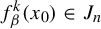 $f^k_\beta (x_0) \in J_n$
. Let
$f^k_\beta (x_0) \in J_n$
. Let $\omega ^{\prime }_i = \omega _i$
for
$\omega ^{\prime }_i = \omega _i$
for $-n \le i \le n$
and
$-n \le i \le n$
and $\omega ^{\prime }_{-n+i} = \beta _i$
for
$\omega ^{\prime }_{-n+i} = \beta _i$
for $-k \le i \le -1$
. Let
$-k \le i \le -1$
. Let $\eta ^{\prime }_i = \hat {\eta }_i$
for
$\eta ^{\prime }_i = \hat {\eta }_i$
for $-m \le i \le m$
and
$-m \le i \le m$
and $\eta ^{\prime }_{-m+i} =$
‘+1’ for
$\eta ^{\prime }_{-m+i} =$
‘+1’ for $-k \le i \le -1$
. We have
$-k \le i \le -1$
. We have $x (G^{m+k} (\chi ^{-(m+k)} (\eta ',\omega ') , x_0)) \in J$
. For
$x (G^{m+k} (\chi ^{-(m+k)} (\eta ',\omega ') , x_0)) \in J$
. For $(\bar {\eta },\bar {\omega },x)$
with
$(\bar {\eta },\bar {\omega },x)$
with $x = X_l (\bar {\omega })$
within distance
$x = X_l (\bar {\omega })$
within distance $\delta $
of
$\delta $
of $x_0$
, concatenate
$x_0$
, concatenate $(\tilde {\eta },\omega )$
on the left with the negative part of
$(\tilde {\eta },\omega )$
on the left with the negative part of $(\bar {\eta },\bar {\omega })$
:
$(\bar {\eta },\bar {\omega })$
: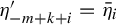 $\eta ^{\prime }_{-m+k+i} = \bar {\eta }_{i}$
for
$\eta ^{\prime }_{-m+k+i} = \bar {\eta }_{i}$
for $i < 0$
and
$i < 0$
and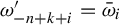 $\omega ^{\prime }_{-n+k+i} = \bar {\omega }_{i}$
for
$\omega ^{\prime }_{-n+k+i} = \bar {\omega }_{i}$
for $i < 0$
. This provides the required positive measure set of sequences.
$i < 0$
. This provides the required positive measure set of sequences.
4.3 Multiple thick metric attractors with intermingled basins
We discuss a slightly different approach and a possible extension leading to examples with multiple thick metric attractors. We will only sketch the constructions and will not provide complete arguments.
The skew product system, corresponding to the iterated function system generated by maps $f_0,f_1$
in the left panel, admits two thick attractors. Taking a random walk on its orbits and adding a composition with additional random choice from maps
$f_0,f_1$
in the left panel, admits two thick attractors. Taking a random walk on its orbits and adding a composition with additional random choice from maps $\phi _0,\phi _1$
, as in the right panel, creates thick metric attractors with intermingled basins.
$\phi _0,\phi _1$
, as in the right panel, creates thick metric attractors with intermingled basins.
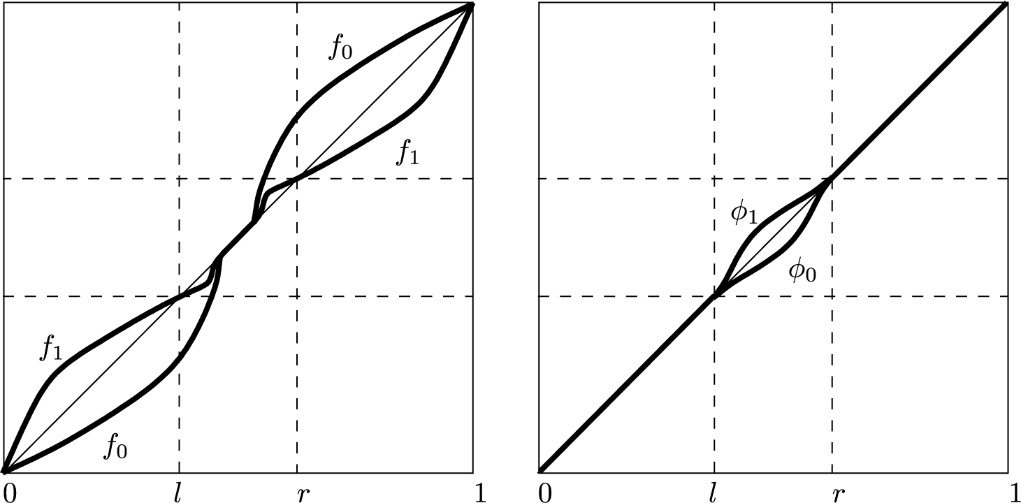
4.3.1 An alternative construction
Take two diffeomorphisms $f_0, f_1$
on
$f_0, f_1$
on $[0,1]$
with graphs as depicted in the left panel of Figure 2. The iterated function system generated by
$[0,1]$
with graphs as depicted in the left panel of Figure 2. The iterated function system generated by $f_0$
and
$f_0$
and $f_1$
provides a skew product system
$f_1$
provides a skew product system  given by $F(\omega ,x) = (\sigma \omega , f_{\omega _0} (x))$
. Take on
$F(\omega ,x) = (\sigma \omega , f_{\omega _0} (x))$
. Take on $\Sigma _2 \times [0,1]$
a reference measure
$\Sigma _2 \times [0,1]$
a reference measure $\nu _{1/2}\times \unicode{x3bb} $
. The map F has two thick attractors: a thick attractor
$\nu _{1/2}\times \unicode{x3bb} $
. The map F has two thick attractors: a thick attractor $\Lambda _l \subset \Sigma _2 \times [0,l]$
and a thick attractor
$\Lambda _l \subset \Sigma _2 \times [0,l]$
and a thick attractor $\Lambda _r \subset \Sigma _2 \times [r,1]$
. With
$\Lambda _r \subset \Sigma _2 \times [r,1]$
. With $\phi _0,\phi _1$
diffeomorphisms on
$\phi _0,\phi _1$
diffeomorphisms on $[0,1]$
, as shown in the right panel of Figure 2, let
$[0,1]$
, as shown in the right panel of Figure 2, let  be given by
 $$ \begin{align*} H(\xi,\eta,\omega,x) = \begin{cases} ( \sigma \xi, \sigma \eta, \sigma \omega, \phi_{\xi_0} \circ f_{\omega_0}(x)), & \eta_0 = +, \\ ( \sigma \xi, \sigma \eta, \sigma^{-1}\omega, \phi_{\xi_0}\circ f_{\omega_{-1}}^{-1}(x)), & \eta_0 = -. \end{cases} \end{align*} $$
Without the maps $\phi _0,\phi _1$
, this is the skew product corresponding to a random walk along orbits of F. The additional compositions with
$\phi _0,\phi _1$
, this is the skew product corresponding to a random walk along orbits of F. The additional compositions with $\phi _0,\phi _1$
provide a random walk between basins of attraction of the two thick metric attractors.
$\phi _0,\phi _1$
provide a random walk between basins of attraction of the two thick metric attractors.
Theorem 4.3. Consider the skew product system H on $\Sigma _2 \times \Omega \times \Sigma _2 \times [0,1]$
. Take
$\Sigma _2 \times \Omega \times \Sigma _2 \times [0,1]$
. Take $\nu _{1/2} \times \nu _p \times \nu _{1/2}\times \unicode{x3bb} $
with
$\nu _{1/2} \times \nu _p \times \nu _{1/2}\times \unicode{x3bb} $
with $1/2 < p < 1$
as a reference measure. The sets
$1/2 < p < 1$
as a reference measure. The sets $\Sigma _2 \times \Omega \times \Lambda _l$
and
$\Sigma _2 \times \Omega \times \Lambda _l$
and $\Sigma _2 \times \Omega \times \Lambda _r$
are thick metric attractors for
$\Sigma _2 \times \Omega \times \Lambda _r$
are thick metric attractors for $H $
with intermingled basins.
$H $
with intermingled basins.
Sketch of proof.
Write $\Pi : \Sigma _2 \times \Omega \times \Sigma _2 \times [0,1] \to [0,1]$
for the coordinate projection to the last coordinate in
$\Pi : \Sigma _2 \times \Omega \times \Sigma _2 \times [0,1] \to [0,1]$
for the coordinate projection to the last coordinate in $[0,1]$
. As before in §4.2, we find that
$[0,1]$
. As before in §4.2, we find that $\Sigma _2 \times \Omega \times \Lambda _l$
and
$\Sigma _2 \times \Omega \times \Lambda _l$
and ${\Sigma _2 \times \Omega \times \Lambda _r}$
are thick metric attractors.
${\Sigma _2 \times \Omega \times \Lambda _r}$
are thick metric attractors.
For any $x \in [0,1]$
,
$x \in [0,1]$
,
 $$ \begin{align} \nu_{1/2} \times \nu_p \times \nu_{1/2} \{ (\xi,\eta,\omega); \Pi H^n (\xi,\eta,\omega,x) \in [0,l]\} &> 0, \end{align} $$
since one can find a cylinder $C \subset \Sigma _2 \times \Omega \times \Sigma _2$
so that
$C \subset \Sigma _2 \times \Omega \times \Sigma _2$
so that $\Pi H^n (\xi ,\eta ,\omega ,x) \in [0,l]$
for
$\Pi H^n (\xi ,\eta ,\omega ,x) \in [0,l]$
for $(\xi ,\eta ,\omega ) \in C$
. Likewise,
$(\xi ,\eta ,\omega ) \in C$
. Likewise,
 $$ \begin{align} \nu_{1/2} \times \nu_p \times \nu_{1/2} \{ (\xi,\eta,\omega); \Pi H^n (\xi,\eta,\omega,x) \in [r,1] \} &> 0. \end{align} $$
From this, we get that for any open set $U \subset \Sigma _2 \times \Omega \times \Sigma _2 \times [0,1]$
, the basin of attraction of
$U \subset \Sigma _2 \times \Omega \times \Sigma _2 \times [0,1]$
, the basin of attraction of $\Sigma _2 \times \Omega \times \Lambda _l$
and of
$\Sigma _2 \times \Omega \times \Lambda _l$
and of $\Sigma _2 \times \Omega \times \Lambda _r$
intersect U in a set of positive reference measure. So, H admits two thick metric attractors with intermingled basins.
$\Sigma _2 \times \Omega \times \Lambda _r$
intersect U in a set of positive reference measure. So, H admits two thick metric attractors with intermingled basins.
4.3.2 Multiple thick metric attractors with intermingled basins
We point out possible extensions to skew product systems with multiple thick metric attractors and also multiple thick metric attractors with mutually intermingled basins. Consider an iterated function system on $[0,1]$
generated by functions
$[0,1]$
generated by functions $f_0,f_1$
with graphs as depicted in Figure 3. There is an invariant interval
$f_0,f_1$
with graphs as depicted in Figure 3. There is an invariant interval $I = [l,r]$
(mapped into itself by both maps). Outside a larger interval
$I = [l,r]$
(mapped into itself by both maps). Outside a larger interval $\tilde {I}$
, the maps are the identity maps.
$\tilde {I}$
, the maps are the identity maps.
We consider an iterated function system generated by diffeomorphisms $f_0$
and
$f_0$
and $f_1$
on
$f_1$
on $[0,1]$
with graphs as depicted. There is an invariant interval
$[0,1]$
with graphs as depicted. There is an invariant interval $[l,r]$
.
$[l,r]$
.
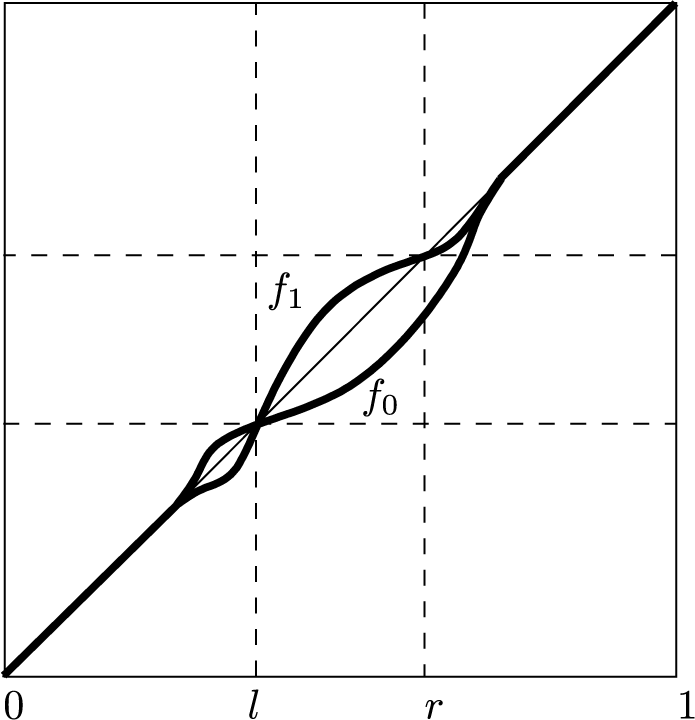
For a positive integer $K_1$
, take
$K_1$
, take $K_1$
mutually disjoint intervals
$K_1$
mutually disjoint intervals $\tilde I_1,\ldots ,\tilde I_{K_1}$
inside
$\tilde I_1,\ldots ,\tilde I_{K_1}$
inside $\mathbb {T}$
, with subintervals
$\mathbb {T}$
, with subintervals $I_i \subset \tilde I_i$
. Let
$I_i \subset \tilde I_i$
. Let $f_0, f_1$
be diffeomorphisms on
$f_0, f_1$
be diffeomorphisms on $\mathbb {T}$
that are identity maps outside
$\mathbb {T}$
that are identity maps outside $\tilde I_1 \cup \cdots \cup \tilde I_{K_1}$
and on
$\tilde I_1 \cup \cdots \cup \tilde I_{K_1}$
and on $\tilde I_i$
have graphs as depicted in Figure 3. For a second set of intervals
$\tilde I_i$
have graphs as depicted in Figure 3. For a second set of intervals $J_1 \subset \tilde {J}_1,\ldots ,J_{K_2}\subset \tilde {J}_{K_2}$
with the
$J_1 \subset \tilde {J}_1,\ldots ,J_{K_2}\subset \tilde {J}_{K_2}$
with the $\tilde {J}_i$
intervals mutually disjoint, take a similar set of diffeomorphisms
$\tilde {J}_i$
intervals mutually disjoint, take a similar set of diffeomorphisms $g_0,g_1$
on
$g_0,g_1$
on $\mathbb {T}$
. Both iterated function systems, generated by
$\mathbb {T}$
. Both iterated function systems, generated by $\{ f_0,f_1\}$
and
$\{ f_0,f_1\}$
and $\{g_0,g_1\}$
, have corresponding skew product systems. Take the product of these. That is, consider the skew product system
$\{g_0,g_1\}$
, have corresponding skew product systems. Take the product of these. That is, consider the skew product system  defined by
 $$ \begin{align} F(\omega , \zeta , x , y) &= (\sigma \omega , \sigma \zeta , f_{\omega_0} (x) , g_{\zeta_0} (y) ). \end{align} $$
On both of the $\Sigma _{2}$
, we take
$\Sigma _{2}$
, we take $(1/2,1/2)$
-Bernoulli measure
$(1/2,1/2)$
-Bernoulli measure $\nu _{1/2}$
. The skew product system
$\nu _{1/2}$
. The skew product system $(\omega ,x)\mapsto (\sigma \omega ,f_{\omega _0} (x))$
has
$(\omega ,x)\mapsto (\sigma \omega ,f_{\omega _0} (x))$
has $K_1$
thick attractors
$K_1$
thick attractors $\Lambda _i \subset \Sigma _2 \times I_i$
. The skew product system
$\Lambda _i \subset \Sigma _2 \times I_i$
. The skew product system $(\zeta ,y)\mapsto (\sigma \zeta ,g_{\zeta _0} (y))$
has
$(\zeta ,y)\mapsto (\sigma \zeta ,g_{\zeta _0} (y))$
has $K_2$
thick attractors
$K_2$
thick attractors $\Xi _j \subset \Sigma _2 \times J_j$
. As in [Reference Ilyashenko21], one can show that F admits
$\Xi _j \subset \Sigma _2 \times J_j$
. As in [Reference Ilyashenko21], one can show that F admits $K_1 K_2$
thick attractors
$K_1 K_2$
thick attractors $\Lambda _i\times \Xi _j \subset \Sigma _2 \times \Sigma _2 \times I_i \times J_j$
,
$\Lambda _i\times \Xi _j \subset \Sigma _2 \times \Sigma _2 \times I_i \times J_j$
, $1 \le i \le K_1, 1 \le j \le K_2$
.
$1 \le i \le K_1, 1 \le j \le K_2$
.
To construct examples of systems with thick metric attractors and mutually intermingled basins, we use the above strategy of introducing random walks along orbits and compose with additional random walks outside the squares $I_i \times J_j$
,
$I_i \times J_j$
, $1 \le i \le K_1, 1 \le j \le K_2$
. Write
$1 \le i \le K_1, 1 \le j \le K_2$
. Write
 $$ \begin{align*} \mathcal{I}_x = \bigcup_{\{1\le i \le K_1\}} I_{i}\times \mathbb{T},\quad \mathcal{I}_y = \bigcup_{\{1\le j \le K_2\}} \mathbb{T} \times I_{j}, \end{align*} $$
and
 $$ \begin{align*}\mathcal{K}_x = \mathbb{T}^2 \setminus \mathcal{I}_x, \quad \mathcal{K}_y = \mathbb{T}^2 \setminus \mathcal{I}_y. \end{align*} $$
Take a diffeomorphism $h_0$
, near the identity map, of the form
$h_0$
, near the identity map, of the form $ h_0 (x,y) = (x + \phi ^x (x,y), y), $
where
$ h_0 (x,y) = (x + \phi ^x (x,y), y), $
where $\phi ^x = 0$
on
$\phi ^x = 0$
on $\mathcal {I}_y$
and
$\mathcal {I}_y$
and $\phi ^x> 0$
on
$\phi ^x> 0$
on $\mathcal {K}_y$
. Let
$\mathcal {K}_y$
. Let $h_1 = h_0^{-1}$
. Take another diffeomorphism
$h_1 = h_0^{-1}$
. Take another diffeomorphism $h_2$
, near the identity map, of the form
$h_2$
, near the identity map, of the form $ h_2 (x,y) = (x, y + \phi ^y (x,y)), $
where
$ h_2 (x,y) = (x, y + \phi ^y (x,y)), $
where $\phi ^y = 0$
on
$\phi ^y = 0$
on $\mathcal {I}_x$
and
$\mathcal {I}_x$
and $\phi ^y> 0$
on
$\phi ^y> 0$
on $\mathcal {K}_x$
. Let
$\mathcal {K}_x$
. Let $h_3 = h_2^{-1}$
. For
$h_3 = h_2^{-1}$
. For $i = 1,2,3,4$
, let
$i = 1,2,3,4$
, let  be given by
 $$ \begin{align*} H_i ( \omega,\zeta , x ,y) = (\omega,\zeta, h_i(x,y)). \end{align*} $$
Define  by
by
 $$ \begin{align*} H(\xi , \eta , \omega,\zeta,x,y) = (\sigma \xi , \sigma \eta , H_{\xi_0} \circ F^{\eta_0} (\omega,\zeta,x,y)). \end{align*} $$
Endow $\Sigma _4$
with
$\Sigma _4$
with $(1/4,1/4,1/4,1/4)$
-Bernoulli measure
$(1/4,1/4,1/4,1/4)$
-Bernoulli measure $\nu _{1/4,1/4,1/4,1/4}$
and
$\nu _{1/4,1/4,1/4,1/4}$
and $\Omega $
with
$\Omega $
with $(p,1-p)$
-Bernoulli measure
$(p,1-p)$
-Bernoulli measure $\nu _p$
for
$\nu _p$
for $1/2 < p < 1$
.
$1/2 < p < 1$
.
Theorem 4.4. Consider the skew product system H on $\Sigma _4 \times \Omega \times \Sigma _2 \times \Sigma _2 \times \mathbb {T}^2$
. Take
$\Sigma _4 \times \Omega \times \Sigma _2 \times \Sigma _2 \times \mathbb {T}^2$
. Take $\nu _{1/4,1/4,1/4,1/4}\times \nu _p \times \nu _{1/2} \times \nu _{1/2} \times \unicode{x3bb} $
as a reference measure. The sets
$\nu _{1/4,1/4,1/4,1/4}\times \nu _p \times \nu _{1/2} \times \nu _{1/2} \times \unicode{x3bb} $
as a reference measure. The sets $\Sigma _4 \times \Omega \times \Lambda _i\times \Xi _j$
,
$\Sigma _4 \times \Omega \times \Lambda _i\times \Xi _j$
, $1 \le i \le K_1, 1 \le j \le K_2$
are thick metric attractors for
$1 \le i \le K_1, 1 \le j \le K_2$
are thick metric attractors for $H $
with mutually intermingled basins.
$H $
with mutually intermingled basins.
Sketch of proof.
The proof follows the lines of Theorem 4.3. Properties (4.2) and (4.3) get replaced by the following. For any $(x,y) \in \mathbb {T}^2$
, there is a cylinder in
$(x,y) \in \mathbb {T}^2$
, there is a cylinder in $\Sigma _4 \times \Omega \times \Sigma _2 \times \Sigma _2$
so that the torus coordinate of
$\Sigma _4 \times \Omega \times \Sigma _2 \times \Sigma _2$
so that the torus coordinate of $H^n (\xi , \eta , \omega ,\zeta ,x,y)$
is in a given square
$H^n (\xi , \eta , \omega ,\zeta ,x,y)$
is in a given square $I_i \times J_j \subset \mathcal {I}_x \cap \mathcal {I}_y$
.
$I_i \times J_j \subset \mathcal {I}_x \cap \mathcal {I}_y$
.
Acknowledgments
The authors thank Shaobo Gan, Yi Shi, and Amin Talebi for useful conversations. A.F. is partially supported by IPM 1404340211 and INSF 4001845.

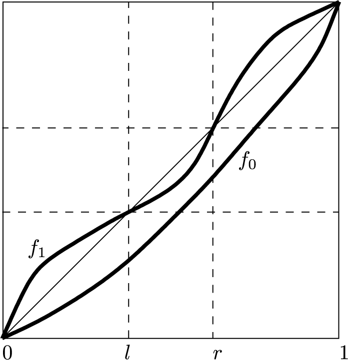


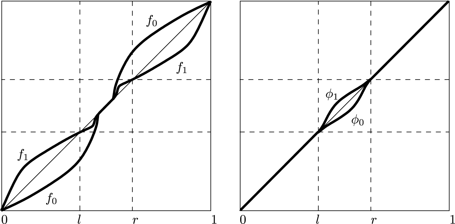


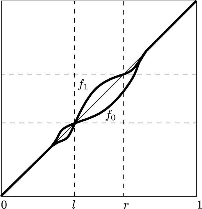


 Open access

