


1. Introduction
Mixing is the process of evolution of constituent concentrations from an initial state of segregation to a final state of homogeneity (Villermaux Reference Villermaux2019). Usually, the influence of turbulence on the mixing of passive scalars is studied to quantify turbulent mixing (Sreenivasan Reference Sreenivasan2019). The evolution of the concentration ( $c$
) of a passive scalar is governed by the advection and molecular diffusion terms as shown in (1.1). Molecular diffusion acts across the interface and reduces the mean value of concentration gradients (Eckart Reference Eckart1948). In the absence of advection, mixing by molecular diffusion occurs at a relatively slow rate (Tennekes & Lumley Reference Tennekes and Lumley1972). Any action that affects the advective term of (1.1) is termed as ‘stirring’. Stirring enhances the mixing process by increasing the mean value of gradients and increases the area across which molecular diffusion occurs (Eckart Reference Eckart1948). Mixing comprising of both stirring and molecular diffusion can be split into two regimes: the regime where stirring dominates over molecular diffusion and the regime where molecular diffusion becomes the significant contributor to mixing (Meunier & Villermaux Reference Meunier and Villermaux2003; Sreenivasan Reference Sreenivasan2019). In this work, we investigate the stirring effect of nonlinear acoustic waves (weak shock waves) and analyse the mechanism by which shock waves enhance the mixing process.
$c$
) of a passive scalar is governed by the advection and molecular diffusion terms as shown in (1.1). Molecular diffusion acts across the interface and reduces the mean value of concentration gradients (Eckart Reference Eckart1948). In the absence of advection, mixing by molecular diffusion occurs at a relatively slow rate (Tennekes & Lumley Reference Tennekes and Lumley1972). Any action that affects the advective term of (1.1) is termed as ‘stirring’. Stirring enhances the mixing process by increasing the mean value of gradients and increases the area across which molecular diffusion occurs (Eckart Reference Eckart1948). Mixing comprising of both stirring and molecular diffusion can be split into two regimes: the regime where stirring dominates over molecular diffusion and the regime where molecular diffusion becomes the significant contributor to mixing (Meunier & Villermaux Reference Meunier and Villermaux2003; Sreenivasan Reference Sreenivasan2019). In this work, we investigate the stirring effect of nonlinear acoustic waves (weak shock waves) and analyse the mechanism by which shock waves enhance the mixing process.
 \begin{equation} \frac {\partial c}{\partial t} +\boldsymbol {u} \boldsymbol {\cdot } \boldsymbol {\nabla } c = D \boldsymbol {\nabla }^{2} c. \end{equation}
Dimotakis (Reference Dimotakis2005) classifies the mixing process into three levels based on the effect of the mixing constituents on the flow dynamics. The mixing of passive scalars is called level-1 mixing, where the mixing constituents have no effect on the flow dynamics irrespective of the coupling due to density gradients. Examples involve the mixing of pollutants, dyes, smoke particles, etc. in fluid. The mixing of active scalars is termed as level-2 mixing, where the mixing process is coupled with the flow dynamics through density gradients. Rayleigh–Taylor and Ritchymer–Meshkov instabilities (RMI) (Richtmyer Reference Richtmyer1954; Meshkov Reference Meshkov1969) are examples of level-2 mixing. Mixing that proceeds with changes in fluid composition is called level-3 mixing. Combustion and detonations are some of the best examples of level-3 mixing. There exists an abundant literature on the mixing of passive scalars in both incompressible and compressible flow fields. Experimental studies on the mixing of passive scalars show that scalar gradients decay with time, and the role of vorticity in turbulent fields is to sustain scalar gradients (Buch & Dahm Reference Buch and Dahm1996). Meunier & Villermaux (Reference Meunier and Villermaux2003) study the mixing of a passive scalar blob using a diffusing Lamb–Oseen type vortex, and show that the changes in concentration can be used to indicate the time in which the effect of stirring is dominant. They identify ‘mixing time’ as an indicator to denote the time during which the action of stirring is dominant over molecular diffusion. They show that the maximum concentration grows linearly until a mixing time is reached, after which it decays in time as $t^{-3/2}$
. Schumacher & Sreenivasan (Reference Schumacher and Sreenivasan2005) derive a relation between the geometrical properties and the mixing statistics of passive scalars using direct numerical simulations (DNS) of a stochastically forced isotropic turbulent field. They relate the area-to-volume ratio to the passive scalar concentration fluctuations and show that the fluctuations mostly follow a Gaussian distribution. Ni (Reference Ni2016) reports that the convolution of scalar fields in forced compressible turbulent flow fields is more pronounced in forcing schemes with a higher ratio of solenoidal-to-dilational components. In a similar study, John et al. (Reference John, Donzis and Sreenivasan2019) show that the breakdown of the passive scalar field depends on the solenoidal components and that the role of compressibility is negligible in the mixing of passive scalars. Gao et al. (Reference Gao, Bermejo-Moreno and Larsson2020) challenge the idea of negligible compressibility effects on mixing by showing the alignment of shock with scalar gradients affects mixing in a canonical shock–turbulence interaction configuration. However, only a few studies exist that analyse the level-2 and level-3 mixing in compressible flows. In this work, we analyse the level-2 mixing of two non-reacting fluids of different densities and study the effect of density inhomogeneity on mixing and flow dynamics in a randomly forced shock-wave field in a two-dimensional set-up.
$t^{-3/2}$
. Schumacher & Sreenivasan (Reference Schumacher and Sreenivasan2005) derive a relation between the geometrical properties and the mixing statistics of passive scalars using direct numerical simulations (DNS) of a stochastically forced isotropic turbulent field. They relate the area-to-volume ratio to the passive scalar concentration fluctuations and show that the fluctuations mostly follow a Gaussian distribution. Ni (Reference Ni2016) reports that the convolution of scalar fields in forced compressible turbulent flow fields is more pronounced in forcing schemes with a higher ratio of solenoidal-to-dilational components. In a similar study, John et al. (Reference John, Donzis and Sreenivasan2019) show that the breakdown of the passive scalar field depends on the solenoidal components and that the role of compressibility is negligible in the mixing of passive scalars. Gao et al. (Reference Gao, Bermejo-Moreno and Larsson2020) challenge the idea of negligible compressibility effects on mixing by showing the alignment of shock with scalar gradients affects mixing in a canonical shock–turbulence interaction configuration. However, only a few studies exist that analyse the level-2 and level-3 mixing in compressible flows. In this work, we analyse the level-2 mixing of two non-reacting fluids of different densities and study the effect of density inhomogeneity on mixing and flow dynamics in a randomly forced shock-wave field in a two-dimensional set-up.
Ritchymer–Meshkov instabilities refer to the growth of perturbations in the interface between two fluids of different densities under the influence of an impulsive acceleration. Ritchymer–Meshkov instabilities are observed in various man-made applications such as inertial-confinement fusion and supersonic combustion (Thomas & Kares Reference Thomas and Kares2012; Yang et al. Reference Yang, Kubota and Zukoski1993; Zhou et al. Reference Zhou2021), as well as naturally occurring phenomena in astrophysics (Burrows Reference Burrows2000; Arnett Reference Arnett2000; Zhou Reference Zhou2017). In cases where shock waves are used for impulsively accelerating the interface, the baroclinic vorticity generated at the interface by the misalignment of pressure gradients and density gradients triggers the growth of perturbations on the interface. The growth of these perturbations triggers other instabilities like Kelvin–Helmholtz instabilities (KHIs), leading to enhanced mixing (Brouillette Reference Brouillette2002; Zhou Reference Zhou2024). The RMI enhanced mixing plays an important role in the design of inertial-confinement fusion reactors (Thomas & Kares Reference Thomas and Kares2012; Zhou et al. Reference Zhou, Sadler and Hurricane2025), and the combustion chambers of supersonic air-breathing engines (Yang et al. Reference Yang, Kubota and Zukoski1993). The change in interface profile caused by RMI is used to develop stellar evolution models to explain the evolution of supernovae explosions (Burrows Reference Burrows2000; Arnett Reference Arnett2000). Ritchymer–Meshkov instabilities are also the fundamental process for studying shock–flame interactions, where the density difference between the two species is used to model burnt and unburnt fuel mixtures, and the passage of shock waves is used to study the flame propagation and the formation of detonation waves (Al-Thehabey Reference Al-Thehabey2020). Primarily, the interfacial mixing and the dynamics of the interface are studied in RMI. Yu et al. (Reference Yu, Liu and Liu2021) show that density gradients across the interface govern the mixing rate. They derive an exact mixing rate expression and show the difference in mixing rates during different stages of RMI. Gao et al. (2016) use Favre averaging of mass fraction to derive the growth rate of the mixing zone width and show that compressibility suppresses the mixing rate for a single pass RMI case. They also report a reduction in the role of the diffusion term in mixing with time. The interface dynamics in RMI are explained in terms of the kinematics of the large-scale coherent structures: spikes (penetration of denser fluid into lighter fluid) and bubbles (penetration of lighter fluid into denser fluid). Zhang (Reference Zhang1998) uses the Layzer-type model (infinite density ratio across the interface) to show that spikes and bubbles have different growth rates. Herrmann et al. (Reference Herrmann, Moin and Abarzhi2008) report that bubbles across interfaces of similar density differences move faster and flatten slower compared with interfaces of higher density differences. They conclude that the evolution of the interface is a non-local and multiscale process. Li et al. (Reference Li, Tian, He and Zhang2021) develop an analytical model to explain the compression and stretching effect of the mixing layer for a single passage of shock wave. They also show that the mixing triggered by RMI lasts even after the passage of the shockwave. In the present work, we use stochastically forced shock waves to induce multimodal perturbations on the interface. We study the mixing induced by such shock waves across interfaces of different density ratios. To this end, we use a simplified two-dimensional model to analyse the mixing characteristics and interface dynamics resulting from continuous and stochastic forcing of a set-up resembling that of RMI using shock-resolved DNS of the fully compressible Navier–Stokes equations.
In this work, we analyse the mixing of active scalars driven by random shock waves. We consider binary mixtures of two non-reacting species with different density ratios. Throughout, we consider a circular shaped inhomogeneity (blob) with a smaller area than the rest of the domain. In § 2, we discuss the governing equations we use to study the mixing enhancement effect of shock waves. We also discuss the details of the numerical set-up and the parameters used to carry out the shock-resolved DNS. In § 3, we first discuss the effect of density gradients on the diffusion of active scalar without shock waves. We use a simplified one-dimensional (1-D) nonlinear diffusion equation to show that the direction of the density gradients affects the evolution of mass fraction due to nonlinear diffusion. We next show the stirring effect of shock waves and its role in enhancing the mixing. We also show the role of baroclinicity in increasing the perimeter across which diffusion occurs before concluding with a summary of our findings in § 4.
2. Governing equations and numerical simulations
In this section, we discuss the governing equations and the numerical method used to study the mixing of two non-reacting species by stochastically forced shock waves. We use the previously developed forcing scheme for generating a random shock-wave field (Jossy & Gupta Reference Jossy and Gupta2023) and summarise it below along with the parameter space.
We use the dimensionless form of the Navier–Stokes and species equation to analyse the mixing of active scalars by shock waves. A non-reacting binary mixture is used to create different density inhomogeneities by varying the molecular weight ( $W_{i}$
) of the species. The dimensionless equations of the density
$W_{i}$
) of the species. The dimensionless equations of the density $\rho$
, velocity
$\rho$
, velocity $\boldsymbol {u}$
, pressure
$\boldsymbol {u}$
, pressure $p$
and concentration of the
$p$
and concentration of the $i^{\mathrm {th}}$
species
$i^{\mathrm {th}}$
species $Y_i$
(mass fraction) are given by
$Y_i$
(mass fraction) are given by
 \begin{equation} \frac {\partial \rho }{ \partial t} + \boldsymbol {\nabla }\boldsymbol {\cdot }(\rho \boldsymbol {u}) =0 , \end{equation}
 \begin{equation} \frac {\partial \boldsymbol {u} }{\partial t} + \boldsymbol {u} \boldsymbol {\cdot } \boldsymbol {\nabla } \boldsymbol {u} + \frac {\boldsymbol {\nabla } p}{\rho } = \frac {1}{ \rho {Re}_{{ac}} } \left ( \boldsymbol {\nabla }\boldsymbol {\cdot }( 2 \mu \boldsymbol {S} )\right ) + \frac {1}{ \rho {Re}_{{ac}} } \left ( \boldsymbol {\nabla }\boldsymbol {\cdot } \left ( \kappa - \frac {2 \mu }{3} \right ) \boldsymbol {D} \right ) + \boldsymbol {F} , \end{equation}
 \begin{equation} \frac {\partial p}{\partial t} + \boldsymbol {u} \boldsymbol {\cdot } \boldsymbol {\nabla } p + \gamma p\boldsymbol {\nabla } \boldsymbol {\cdot } \boldsymbol {u} = \frac {1}{{Re}_{{ac}} \hspace {0.8mm} {Pr}} \boldsymbol {\nabla } \boldsymbol {\cdot } (\alpha \boldsymbol {\nabla } T) + \frac {\gamma -1 }{{Re}_{{ac}}}\left (2 \mu \boldsymbol {S}:\boldsymbol {S} +\left ( \kappa -\frac {2 \mu }{3}\right )\boldsymbol {D}:\boldsymbol {D} \right )\! , \end{equation}
 \begin{equation} \frac {\partial Y_{i}}{\partial t} + \boldsymbol {u} \boldsymbol {\cdot } \boldsymbol {\nabla } Y_{i} = \frac {1}{\rho \hspace {0.8mm} {Re}_{{ac}} {Sc}\hspace {0.8mm} } \boldsymbol {\nabla } \boldsymbol {\cdot } \left ( \rho \frac {W_{i}}{W} \boldsymbol {\nabla } X_{i}\right ), \end{equation}
where $W$
is the mean molecular mass of the mixture, and
$W$
is the mean molecular mass of the mixture, and $X_i$
is the mole fraction of the
$X_i$
is the mole fraction of the ${i}^{th}$
species related to the mass fraction
${i}^{th}$
species related to the mass fraction $Y_i$
as
$Y_i$
as
 \begin{equation} X_{i} = \frac {W}{W_{i}} Y_{i} . \end{equation}
We combine the above equations using the dimensionless equation of state for an ideal gas mixture,
 \begin{equation} \gamma p = \frac {\rho }{W} T, \end{equation}
where
 \begin{equation} \frac {1}{W} = \frac {Y_{1}}{W_{1}} + \frac {Y_{2}}{W_{2}}. \end{equation}
We use the pressure equation (2.3) derived from the conservative energy equation and the internal energy equation for an ideal gas (Kundu et al. Reference Kundu, Cohen and Dowling2015). We note that solving pressure equation is equivalent to solving the internal energy equation for a perfect gas. Moreover, the pressure equation has been extensively used previously in mixing and compressible turbulence studies spanning all ranges of Mach numbers (Sarkar et al. Reference Sarkar, Erlebacher, Hussaini and Kreiss1991; Sarkar Reference Sarkar1995; Pantano et al. Reference Pantano, Sarkar and Williams2003). In (2.2) and (2.3), $\boldsymbol {S}$
and
$\boldsymbol {S}$
and $\boldsymbol {D}$
are the strain rate and dilatation tensors, respectively, given by
$\boldsymbol {D}$
are the strain rate and dilatation tensors, respectively, given by
 \begin{equation} \boldsymbol {S} = \frac {1}{2}\big(\boldsymbol {\nabla }\boldsymbol {u} + \boldsymbol {\nabla }\boldsymbol {u}^T\big), \,\boldsymbol {D} = \left (\boldsymbol {\nabla }\boldsymbol {\cdot }\boldsymbol {u} \right ) \boldsymbol {I} . \end{equation}
The fluid properties such as dynamic viscosity ( $\mu$
), bulk viscosity (
$\mu$
), bulk viscosity ( $\kappa$
) and thermal conductivity (
$\kappa$
) and thermal conductivity ( $\alpha$
) are all dimensionless. The flow properties are governed by the dimensionless numbers, the acoustic Reynolds number (
$\alpha$
) are all dimensionless. The flow properties are governed by the dimensionless numbers, the acoustic Reynolds number ( ${Re}_{{ac}}$
), the Prandlt number (
${Re}_{{ac}}$
), the Prandlt number ( ${Pr}$
) and the Schmidt number (
${Pr}$
) and the Schmidt number ( ${Sc}$
) defined as
${Sc}$
) defined as
 \begin{equation} {Re}_{{ac}} = \frac {\rho _{m} c_{m} L_{m}} {\mu _{m}}, \hspace {2 mm} {Pr} = \frac { \gamma \mu _{m} \tilde {R} }{(\gamma - 1) W_{m} \alpha _{m}},\hspace {2 mm} {Sc} = \frac {\mu _{m}}{\rho _{m} \lambda _{m}}. \end{equation}
The flow field parameters are scaled using the characteristic dimensional quantities which are denoted by the subscript $()_{m}$
. The velocity is scaled using the characteristic speed of sound
$()_{m}$
. The velocity is scaled using the characteristic speed of sound $c_{m}$
, and
$c_{m}$
, and $\tilde {R}$
,
$\tilde {R}$
, $\mu _{m}, \alpha _{m}$
and
$\mu _{m}, \alpha _{m}$
and $\lambda _{m}$
denote the universal gas constant, dimensional viscosity, thermal conductivity and diffusion coefficient, respectively. Since we use dimensionless equations in our numerical simulations, the specific values of the characteristic scales hold no significance. We also assume that the heat capacities of both the species are the same.
$\lambda _{m}$
denote the universal gas constant, dimensional viscosity, thermal conductivity and diffusion coefficient, respectively. Since we use dimensionless equations in our numerical simulations, the specific values of the characteristic scales hold no significance. We also assume that the heat capacities of both the species are the same.
We refer the reader to our earlier work (Jossy & Gupta Reference Jossy and Gupta2023) for a detailed derivation of the dimensionless governing equations (2.1)–(2.3) and the appropriate characteristic scales of the quantities. The forcing term $\boldsymbol {F}$
in (2.2) is used to generate shock waves. For species diffusion, we use the Hirschfelder and Curtiss approximation (Hirschfelder et al. Reference Hirschfelder, Curtiss and Bird1964; Poinsot & Veynante Reference Poinsot and Veynante2005) in (2.4) with a constant equivalent diffusion coefficient. As we discuss in later sections, the nonlinear diffusive flux in (2.4) results in a translation of the active scalar interface, resulting in an expansion or contraction of the inhomogeneities, depending on the value of the molecular mass ratio.
$\boldsymbol {F}$
in (2.2) is used to generate shock waves. For species diffusion, we use the Hirschfelder and Curtiss approximation (Hirschfelder et al. Reference Hirschfelder, Curtiss and Bird1964; Poinsot & Veynante Reference Poinsot and Veynante2005) in (2.4) with a constant equivalent diffusion coefficient. As we discuss in later sections, the nonlinear diffusive flux in (2.4) results in a translation of the active scalar interface, resulting in an expansion or contraction of the inhomogeneities, depending on the value of the molecular mass ratio.
2.1. Fourier pseudospectral simulations
We perform shock-resolved DNS of the fully compressible two-dimensional Navier–Stokes equations (2.1)–(2.3) and the species equation (2.4) using an MPI (message passing interface) parallelised Fourier pseudospectral solver (Boyd Reference Boyd2001). We note that both the momentum (2.2) and the pressure equation (2.3) are used in the non-conservative form in this work. Since the derivatives are calculated using the exact relation $\widehat {\nabla \phi } = i\textbf{k}\hat {\phi }$
(where
$\widehat {\nabla \phi } = i\textbf{k}\hat {\phi }$
(where $\hat {\phi }$
denotes the Fourier transform of a field
$\hat {\phi }$
denotes the Fourier transform of a field $\phi$
), the non-conservative form of the equations poses no limitations. We use the Runge–Kutta fourth-order scheme for time stepping and ensure numerical stability using the 2/3 deliasing method in the nonlinear terms only to eliminate the aliasing errors. As we show later, nonlinearities are negligible for length scales much larger than the length scale below which the aliasing errors are removed. For all the simulations discussed in the work, we consider 3072 Fourier modes in each direction such that the nonlinear terms are resolved until
$\phi$
), the non-conservative form of the equations poses no limitations. We use the Runge–Kutta fourth-order scheme for time stepping and ensure numerical stability using the 2/3 deliasing method in the nonlinear terms only to eliminate the aliasing errors. As we show later, nonlinearities are negligible for length scales much larger than the length scale below which the aliasing errors are removed. For all the simulations discussed in the work, we consider 3072 Fourier modes in each direction such that the nonlinear terms are resolved until $k_{{max}}=1024$
. We show in § 2.2 and the convergence study in appendix A that the resolution is sufficient to resolve all the scales for the values of the energy injection rate (
$k_{{max}}=1024$
. We show in § 2.2 and the convergence study in appendix A that the resolution is sufficient to resolve all the scales for the values of the energy injection rate ( $\varepsilon$
in (2.13)) used in this work. Each simulation is run using 256 cores consuming approximately
$\varepsilon$
in (2.13)) used in this work. Each simulation is run using 256 cores consuming approximately $10^{5}$
core hours. We consider constant viscosity (
$10^{5}$
core hours. We consider constant viscosity ( $\mu =1$
) and thermal conductivity (
$\mu =1$
) and thermal conductivity ( $\alpha =1$
) for all our simulations and ignore bulk viscosity (
$\alpha =1$
) for all our simulations and ignore bulk viscosity ( $\kappa = 0$
) for simplicity. For all simulations, we consider
$\kappa = 0$
) for simplicity. For all simulations, we consider ${Pr} = {Sc} = 0.7$
, such that the molecular diffusion and heat diffusivity remain the same. We initialise our simulations using quiescent (
${Pr} = {Sc} = 0.7$
, such that the molecular diffusion and heat diffusivity remain the same. We initialise our simulations using quiescent ( $\boldsymbol {u} =0$
), isobaric (uniform pressure) and isothermal (uniform temperature) conditions with a circular blob of radius
$\boldsymbol {u} =0$
), isobaric (uniform pressure) and isothermal (uniform temperature) conditions with a circular blob of radius $\pi /2$
. We specify the species having a circular distribution using the
$\pi /2$
. We specify the species having a circular distribution using the $\tanh$
function to specify the initial concentration field, as follows:
$\tanh$
function to specify the initial concentration field, as follows:
 \begin{equation} Y_{c} =\frac {1}{2} \left [1 - \textrm{tanh}\left ( \frac {1}{\delta } \left (\sqrt { (x - \pi )^{2} + (y - \pi )^2} - \frac {\pi }{2} \right )\right ) \right ] . \end{equation}
The species constituting the blob has density $\rho _{c}$
and the surrounding species has density
$\rho _{c}$
and the surrounding species has density $\rho _{s}$
. We use subscript
$\rho _{s}$
. We use subscript $()_c$
to indicate the species inside the circular blob and the subscript
$()_c$
to indicate the species inside the circular blob and the subscript $()_s$
to denote the surrounding species. We use the parameter value
$()_s$
to denote the surrounding species. We use the parameter value $\delta = 1/15$
in (2.10) to obtain a steep but smooth concentration distribution to achieve a diffused thin interface. The parameter
$\delta = 1/15$
in (2.10) to obtain a steep but smooth concentration distribution to achieve a diffused thin interface. The parameter $\delta$
represents a characteristic interface thickness and will be used later to calculate the apparent perimeter of the interface during mixing.
$\delta$
represents a characteristic interface thickness and will be used later to calculate the apparent perimeter of the interface during mixing.
The forcing $\boldsymbol {F}$
in (2.2) is similar to the one used by Jossy & Gupta (Reference Jossy and Gupta2023). For completeness, we provide a brief overview here. The forcing
$\boldsymbol {F}$
in (2.2) is similar to the one used by Jossy & Gupta (Reference Jossy and Gupta2023). For completeness, we provide a brief overview here. The forcing $\boldsymbol {F}$
is defined in the Fourier space and computed using four statistically independent Uhlenbeck–Ornstein (UO) (Eswaran & Pope Reference Eswaran and Pope1988) processes (
$\boldsymbol {F}$
is defined in the Fourier space and computed using four statistically independent Uhlenbeck–Ornstein (UO) (Eswaran & Pope Reference Eswaran and Pope1988) processes ( $a_{i,\boldsymbol {k}} (t)$
for
$a_{i,\boldsymbol {k}} (t)$
for $i = 1,2,3$
and
$i = 1,2,3$
and $4$
), satisfying the following conditions:
$4$
), satisfying the following conditions:
 \begin{align} &\left \langle a_{i, \boldsymbol {k}}(t)\right \rangle = 0 , \end{align}
 \begin{align} &\big\langle {a}_{i, \boldsymbol {k}}(t) {a}_{j, \boldsymbol {k}}^{*}(t+s)\big \rangle = 2 \sigma ^{2} \boldsymbol {\delta _{ij}}\exp (-s/T_L) , \end{align}
where $\left \langle \cdot \right \rangle$
denotes the ensemble average,
$\left \langle \cdot \right \rangle$
denotes the ensemble average, $()^*$
denotes the complex conjugate,
$()^*$
denotes the complex conjugate, $\sigma ^2$
is the variance, and
$\sigma ^2$
is the variance, and $T_L$
is the forcing timescale. To prevent any direct effect of energy injection at small length scales, we restrict our forcing to larger scales within the band of wavenumbers
$T_L$
is the forcing timescale. To prevent any direct effect of energy injection at small length scales, we restrict our forcing to larger scales within the band of wavenumbers $0 \lt |\boldsymbol {k}| \lt k_{F}$
, where
$0 \lt |\boldsymbol {k}| \lt k_{F}$
, where $k_{F} = 5$
in all our simulations. The total rate of energy injection
$k_{F} = 5$
in all our simulations. The total rate of energy injection $\varepsilon$
is a function of the variance
$\varepsilon$
is a function of the variance $\sigma ^{2}$
, the time scale
$\sigma ^{2}$
, the time scale $T_{L}$
of the UO process, and the number of wave vectors within the forcing band
$T_{L}$
of the UO process, and the number of wave vectors within the forcing band $N_{F}$
and is given by
$N_{F}$
and is given by
 \begin{equation} \varepsilon = 4 N_{F} T_{L} \sigma ^{2}. \end{equation}
The forcing vector in the Fourier space can be obtained by combining the four independent processes as
 \begin{equation} \widehat {\boldsymbol {a}}_{\boldsymbol {k}} = \left (a_{1,\boldsymbol {k}} + i a_{2,\boldsymbol {k}}, a_{3,\boldsymbol {k}} + ia_{4,\boldsymbol {k}}\right )^T. \end{equation}
To force only the acoustical component of velocity, we remove the vortical component from $\widehat {\boldsymbol {a}}_{\boldsymbol {k}}$
yielding
$\widehat {\boldsymbol {a}}_{\boldsymbol {k}}$
yielding
 \begin{align} \widehat {\boldsymbol {F}}_{\boldsymbol {k}}(t) = \frac {(\widehat {\boldsymbol {a}}_{\boldsymbol {k}}(t) \cdot \boldsymbol {k})}{|\boldsymbol {k}|^2}\boldsymbol {k}. \end{align}
It has been shown that decaying acoustic wave turbulence has similar behaviour to Burgers turbulence (Gupta & Scalo Reference Gupta and Scalo2018). We speculate that the behaviour of stochastically forced shock waves may be similar to that of two-dimensional forced Burgers turbulence (Cho et al. Reference Cho, Venturi and Karniadakis2014). A detailed comparison between the two is beyond the scope of the current study. In our earlier work (Jossy & Gupta Reference Jossy and Gupta2023), we have used the stochastic forcing method described above to generate a field of isotropic shock waves. The wave energy spectra of the random shock waves generated exhibit identical dependence on the dissipation and the integral length scale as decaying 1-D turbulence (Gupta & Scalo Reference Gupta and Scalo2018) as well as shallow water wave-turbulence (Augier et al. Reference Augier, Mohanan and Lindborg2019). Augier et al. (Reference Augier, Mohanan and Lindborg2019) derive the shallow water wave-turbulence scaling laws assuming isotropy, independent of the dispersive nature of the shallow water waves. Hence, the forcing method mentioned in (2.15) generates a field of isotropic random shock waves whose phasing changes at every time instant in a homogeneous mixture. Reflections of the shock waves at the inhomogeneity interface may introduce some spatial anistropy, a detailed analysis of which is deferred to future studies and is beyond the scope of the current work. As mentioned earlier, in this work, we study the interaction of forced weak shock waves, which induce multimodal perturbations on the inhomogeneity interface separating the two species and thus influencing the active scalar mixing dynamics.
Parameter space for simulations considering only the effect of molecular diffusion without any shock waves along with their indicators.

2.2. Simulation parameters
To study the effect of forced weak shock waves on the mixing of species with different densities, we use the Atwood number ( $At$
), defined as
$At$
), defined as
 \begin{equation} At = \frac {\rho _{s} - \rho _{c}}{\rho _{s} + \rho _{c}} \hspace {1 mm} = \frac {\chi - 1}{\chi + 1} . \end{equation}
We study the effect of shock waves in both a denser mixture ( $\chi \gt 1$
) and a lighter mixture (
$\chi \gt 1$
) and a lighter mixture ( $\chi \lt 1$
), where
$\chi \lt 1$
), where $\chi$
is the density ratio of surrounding species to the blob species. To understand the effect of density gradients on the species diffusion alone, we run one case each of positive and negative Atwood numbers without any shocks and compare them with a passive scalar case. Table 1 shows the parameters of the simulation cases without any shock waves. We study the effect of weak shock waves on mixing for three values of positive and negative Atwood numbers each and compare their mixing dynamics with a passive scalar case. Since each realisation of the stochastic forcing
$\chi$
is the density ratio of surrounding species to the blob species. To understand the effect of density gradients on the species diffusion alone, we run one case each of positive and negative Atwood numbers without any shocks and compare them with a passive scalar case. Table 1 shows the parameters of the simulation cases without any shock waves. We study the effect of weak shock waves on mixing for three values of positive and negative Atwood numbers each and compare their mixing dynamics with a passive scalar case. Since each realisation of the stochastic forcing $\boldsymbol {F}$
is different, the mixing process itself is a stochastic non-equilibrium process. Hence, we simulate additional realisations of the end ranges of the Atwood number, i.e. four realisations of
$\boldsymbol {F}$
is different, the mixing process itself is a stochastic non-equilibrium process. Hence, we simulate additional realisations of the end ranges of the Atwood number, i.e. four realisations of $At = \pm 0.75$
and three realisations of
$At = \pm 0.75$
and three realisations of $At = \pm 0.25$
to show that the mixing characteristics are consistent across Atwood numbers for different realisations of the same forcing parameters. The average of the different realisations is represented by the superscript
$At = \pm 0.25$
to show that the mixing characteristics are consistent across Atwood numbers for different realisations of the same forcing parameters. The average of the different realisations is represented by the superscript $()^{\dagger }$
.
$()^{\dagger }$
.
As mentioned earlier, we choose $k_{{max}} =1024$
to discuss the results of the study. But to show that the chosen resolution is sufficient, we run additional simulations with
$k_{{max}} =1024$
to discuss the results of the study. But to show that the chosen resolution is sufficient, we run additional simulations with $k_{{max}}=768$
and
$k_{{max}}=768$
and $k_{{max}}=1536$
, which are denoted by the superscripts
$k_{{max}}=1536$
, which are denoted by the superscripts $()^{\star }$
and
$()^{\star }$
and $()^{\ddagger }$
, respectively. The details of the convergence study are given in appendix A. Table 2 shows the simulation cases used to study the stirring effect of shock waves. For all simulations, we inject acoustic energy at the rate of
$()^{\ddagger }$
, respectively. The details of the convergence study are given in appendix A. Table 2 shows the simulation cases used to study the stirring effect of shock waves. For all simulations, we inject acoustic energy at the rate of $\varepsilon / 4 N_{F} =1.25 \times 10^{-6}$
to generate weak shock waves (
$\varepsilon / 4 N_{F} =1.25 \times 10^{-6}$
to generate weak shock waves ( $ \langle M \rangle \lt 1.1$
). We run all the realisations for all the cases for sufficiently long times until the effects of molecular diffusion take over the effects of stirring. We run one realisation for all the different Atwood numbers shown in table 2 further close to homogenisation. The smallest length scales generated in the simulations correspond to the shock thickness scale
$ \langle M \rangle \lt 1.1$
). We run all the realisations for all the cases for sufficiently long times until the effects of molecular diffusion take over the effects of stirring. We run one realisation for all the different Atwood numbers shown in table 2 further close to homogenisation. The smallest length scales generated in the simulations correspond to the shock thickness scale $\eta$
(Donzis Reference Donzis2012; Larsson et al. Reference Larsson, Bermejo-Moreno and Lele2013; Gupta & Scalo 2018; Jossy & Gupta Reference Jossy and Gupta2023) and the Batchelor scale
$\eta$
(Donzis Reference Donzis2012; Larsson et al. Reference Larsson, Bermejo-Moreno and Lele2013; Gupta & Scalo 2018; Jossy & Gupta Reference Jossy and Gupta2023) and the Batchelor scale $\eta _B$
, which are related to the acoustic Reynolds number
$\eta _B$
, which are related to the acoustic Reynolds number ${Re}_{ac}$
as
${Re}_{ac}$
as
Parameter space for simulations with stochastically generated shock waves and their corresponding indicators. In the above table, $\langle M \rangle$
represents the area averaged Mach number of the shock waves in the domain,
$\langle M \rangle$
represents the area averaged Mach number of the shock waves in the domain, $\langle \eta \rangle _{t}$
represents the time-averaged shock thickness scale and
$\langle \eta \rangle _{t}$
represents the time-averaged shock thickness scale and $\langle \eta _{B} \rangle$
represents the time averaged Batchelor scale.
$\langle \eta _{B} \rangle$
represents the time averaged Batchelor scale.

 \begin{equation} \eta \sim \frac {1}{{Re}_{{ac}}} ( \varepsilon \ell )^{-1/3} , \quad \eta _{B} = \frac {\eta }{\sqrt {{Sc}}}, \end{equation}
where $\ell = 2/k_F$
is the integral length scale, which represents the mean distance between two shocks. To ensure shock-resolved simulations, we consider
$\ell = 2/k_F$
is the integral length scale, which represents the mean distance between two shocks. To ensure shock-resolved simulations, we consider ${Re}_{{ac}} = 1000$
, such that
${Re}_{{ac}} = 1000$
, such that $ k_{{max}} \eta \gt 1.5$
and follow an even more strict resolution scale for mixing,
$ k_{{max}} \eta \gt 1.5$
and follow an even more strict resolution scale for mixing, $ \eta _{B}/\Delta \gt 0.5$
(Schumacher et al. Reference Schumacher, Sreenivasan and Yeung2005) where
$ \eta _{B}/\Delta \gt 0.5$
(Schumacher et al. Reference Schumacher, Sreenivasan and Yeung2005) where $\Delta$
is given by
$\Delta$
is given by $ 2\sqrt {2} \pi / 3k_{{max}}$
. To show resolution in all our simulations, we calculate the binned density-weighted wave spectral energy
$ 2\sqrt {2} \pi / 3k_{{max}}$
. To show resolution in all our simulations, we calculate the binned density-weighted wave spectral energy $\widehat {E}_{wk}$
and the spectral flux of the wave energy
$\widehat {E}_{wk}$
and the spectral flux of the wave energy $\widehat {\Pi }_{wk}$
whose definitions are given in (2.18) and (2.19), respectively. We direct the reader to previous studies (Miura & Kida Reference Miura and Kida1995; Jossy & Gupta Reference Jossy and Gupta2023) for the detailed derivation of the density-weighted spectral quantities. We use a density-weighted velocity
$\widehat {\Pi }_{wk}$
whose definitions are given in (2.18) and (2.19), respectively. We direct the reader to previous studies (Miura & Kida Reference Miura and Kida1995; Jossy & Gupta Reference Jossy and Gupta2023) for the detailed derivation of the density-weighted spectral quantities. We use a density-weighted velocity $\boldsymbol {w} = \sqrt {\rho } \boldsymbol {u}$
and its wave component obtained upon the Helmholtz decomposition (Miura & Kida Reference Miura and Kida1995; Jossy & Gupta Reference Jossy and Gupta2023). Denoting the Fourier transform of a quantity
$\boldsymbol {w} = \sqrt {\rho } \boldsymbol {u}$
and its wave component obtained upon the Helmholtz decomposition (Miura & Kida Reference Miura and Kida1995; Jossy & Gupta Reference Jossy and Gupta2023). Denoting the Fourier transform of a quantity $\phi$
by
$\phi$
by $\hat {\phi }$
and the complex conjugate by
$\hat {\phi }$
and the complex conjugate by $\hat {\phi }^{*}$
, the density-weighted wave spectral energy
$\hat {\phi }^{*}$
, the density-weighted wave spectral energy $\widehat {E}_{wk}$
and its transfer function
$\widehat {E}_{wk}$
and its transfer function $\widehat {\mathcal {T}}_{wk}$
are obtained as
$\widehat {\mathcal {T}}_{wk}$
are obtained as
 \begin{align} \widehat {E}_{wk} & = \frac {1}{2} \left ( \widehat {\boldsymbol {w}}^{*}_{wk} \cdot \widehat {\boldsymbol {w}}_{wk} + \widehat {\left (p - \frac {1}{\gamma }\right )}_{k}^{*} \widehat {\left (p - \frac {1}{\gamma }\right )}_{k} \right ),\end{align}
 \begin{align} \widehat {\mathcal {T}}_{wk} =&\mathcal {R}\left [\widehat { \boldsymbol {w}}^*_{wk}\cdot \left (\widehat {\frac {\nabla p}{\sqrt {\rho }}}\right )_{k} + \widehat {\left (p - \frac {1}{\gamma }\right )}^*_{k}\widehat {\nabla \cdot \boldsymbol {u}}_{wk}\right ] \nonumber \\ &+\mathcal {R}\left [\hat {\boldsymbol {w}}^*_{wk}\cdot \big(\widehat {\boldsymbol {w}\cdot \nabla \boldsymbol {u}}\big)_{wk} - \widehat {\boldsymbol {w}}^*_{wk}\cdot \left (\widehat {\frac {\left (p - \frac {1}{\gamma }\right )\nabla p}{\sqrt {\rho }}}\right )_{k}\right ] \nonumber \\ &+ \mathcal {R}\left [\gamma \widehat {\left (p - \frac {1}{\gamma }\right )}^*_{k}\left (\widehat {\left (p - \frac {1}{\gamma }\right )\nabla \cdot \boldsymbol {u}}\right )_{wk} + \widehat {\left (p - \frac {1}{\gamma }\right )}^*_{k}\big(\widehat {\boldsymbol {u}\cdot \nabla p}\big)_{wk}\right ], \end{align}
where the subscript $()_{wk}$
denotes the Fourier transform of the wavefield, and
$()_{wk}$
denotes the Fourier transform of the wavefield, and $\mathcal {R}()$
denotes the real part of the quantity. Equations (2.18) and (2.19) are derived using the second-order approximation of (2.1)–(2.3) (see Jossy & Gupta (Reference Jossy and Gupta2023) for a detailed derivation). The term
$\mathcal {R}()$
denotes the real part of the quantity. Equations (2.18) and (2.19) are derived using the second-order approximation of (2.1)–(2.3) (see Jossy & Gupta (Reference Jossy and Gupta2023) for a detailed derivation). The term $p - \frac {1}{\gamma }$
is the change in pressure from the isobaric base state at the dimensionless pressure of
$p - \frac {1}{\gamma }$
is the change in pressure from the isobaric base state at the dimensionless pressure of $1/\gamma$
. Figure 1(a) shows the scaled density-weighted wave energy spectra
$1/\gamma$
. Figure 1(a) shows the scaled density-weighted wave energy spectra $\widehat {E}_{wk}\varepsilon ^{-2/3}\ell ^{-5/3}$
versus the scaled wavenumber
$\widehat {E}_{wk}\varepsilon ^{-2/3}\ell ^{-5/3}$
versus the scaled wavenumber $k\ell$
. Since the forcing acts only within
$k\ell$
. Since the forcing acts only within $0 \lt k\ell \lt 2$
, wave energy in the further wavenumbers highlights forward spectral wave energy cascade due to the nonlinear terms in the governing equations. Since the generated shock waves are weak,
$0 \lt k\ell \lt 2$
, wave energy in the further wavenumbers highlights forward spectral wave energy cascade due to the nonlinear terms in the governing equations. Since the generated shock waves are weak, $\widehat {E}_{wk}$
decays as
$\widehat {E}_{wk}$
decays as $k^{-2}$
before decaying rapidly due to thermoviscous dissipation. Figure 1(b) shows the scaled flux of the spectral wave energy
$k^{-2}$
before decaying rapidly due to thermoviscous dissipation. Figure 1(b) shows the scaled flux of the spectral wave energy $\widehat {\Pi }_{wk}/\varepsilon$
calculated as the cumulative sum of the transfer function
$\widehat {\Pi }_{wk}/\varepsilon$
calculated as the cumulative sum of the transfer function $\widehat {\mathcal {T}}_{wk}$
in (2.19). The spectral flux approaches net dissipation (equal to net energy injection) and then decays after a decade as the wavenumber increases. Unlike hydrodynamic turbulence, thermoviscous dissipation is significant at all scales in a field of random shock waves since the wave energy
$\widehat {\mathcal {T}}_{wk}$
in (2.19). The spectral flux approaches net dissipation (equal to net energy injection) and then decays after a decade as the wavenumber increases. Unlike hydrodynamic turbulence, thermoviscous dissipation is significant at all scales in a field of random shock waves since the wave energy $\sim k^{-2}$
and the dissipation scales as
$\sim k^{-2}$
and the dissipation scales as $k^2\widehat {E}_{wk}$
approximately. Similar values of spectral flux and the net energy injection highlight that the waves generated are nonlinear. Decay of the spectral flux in figure 1 before
$k^2\widehat {E}_{wk}$
approximately. Similar values of spectral flux and the net energy injection highlight that the waves generated are nonlinear. Decay of the spectral flux in figure 1 before $k_{{max}}\ell$
for all the cases shows that nonlinearities become negligible for length scales approaching
$k_{{max}}\ell$
for all the cases shows that nonlinearities become negligible for length scales approaching $1/k_{{max}}$
. Since the dealiasing is used only in the nonlinear terms, any linear dynamics at length scales smaller than
$1/k_{{max}}$
. Since the dealiasing is used only in the nonlinear terms, any linear dynamics at length scales smaller than $1/k_{{max}}$
until
$1/k_{{max}}$
until $1/3072$
are well resolved. In appendix A, we show that the wave energy spectra for
$1/3072$
are well resolved. In appendix A, we show that the wave energy spectra for $k\gt k_{{max}}$
are modified slightly only for
$k\gt k_{{max}}$
are modified slightly only for $At=0.75$
case for
$At=0.75$
case for $k_{{max}}=1536$
. However, the energy in these scales is more than seven orders of magnitude smaller than the integral length scale energy. Hence, these scales have negligible influence on the mixing dynamics, which are governed by the pressure variations leading to baroclinicity (see §§ 3.2 and 3.3). Yet, we show the contours and discuss the effects of weak shock waves on mixing dynamics using
$k_{{max}}=1536$
. However, the energy in these scales is more than seven orders of magnitude smaller than the integral length scale energy. Hence, these scales have negligible influence on the mixing dynamics, which are governed by the pressure variations leading to baroclinicity (see §§ 3.2 and 3.3). Yet, we show the contours and discuss the effects of weak shock waves on mixing dynamics using $At=\pm 0.5$
cases, for which all the scales are resolved for
$At=\pm 0.5$
cases, for which all the scales are resolved for $k_{{max}}$
= 1024 as shown in appendix A.
$k_{{max}}$
= 1024 as shown in appendix A.
Dimensionless scaled density-weighted wave energy $\hat {E}_{wk}$
spectra (a) and spectral flux of wave energy
$\hat {E}_{wk}$
spectra (a) and spectral flux of wave energy $\widehat {\Pi }_{wk}$
(b) of active scalars cases in table 2 averaged over the time interval
$\widehat {\Pi }_{wk}$
(b) of active scalars cases in table 2 averaged over the time interval $t=50$
to
$t=50$
to $t=300$
. The vertical lines in both the figures show the dealiasing limit
$t=300$
. The vertical lines in both the figures show the dealiasing limit $k_{{max}}\ell$
. The spectral flux is negligible beyond the
$k_{{max}}\ell$
. The spectral flux is negligible beyond the $k_{{max}}\ell$
limit highlighting that all the nonlinear scales are resolved. The legends are identical for both the figures. Contours of divergence at different time instances for
$k_{{max}}\ell$
limit highlighting that all the nonlinear scales are resolved. The legends are identical for both the figures. Contours of divergence at different time instances for $At=0.5$
(c).
$At=0.5$
(c).

The variation of density-weighted wave spectra across different Atwood number cases occurs due to the variation in density across the inhomogeneity interface. Stretching and folding of the inhomogeneity generate smaller scales in the interface. However, the scale corresponding to the interface thickness increases due to molecular diffusion. As discussed later in § 3.1, the molecular diffusion term responsible for the diffusion of the interface (later termed as the Laplacian diffusion term) and the molecular diffusion term responsible for the movement of the interface due to the density gradients (later termed as the nonlinear dissipation term) change with the Atwood number (cf. (3.4)). For $At\gt 0$
, the Laplacian diffusion term dominates the nonlinear dissipation term. As
$At\gt 0$
, the Laplacian diffusion term dominates the nonlinear dissipation term. As $At\gt 0$
increases, the Laplacian diffusion coefficient decreases, indicating relatively smaller scales maintained for higher values of
$At\gt 0$
increases, the Laplacian diffusion coefficient decreases, indicating relatively smaller scales maintained for higher values of $At\gt 0$
in figure 1(a). As
$At\gt 0$
in figure 1(a). As $At\lt 0$
decreases, the nonlinear dissipation coefficient increases resulting in more rapid expansion of the interface. This results in more collisions of the shock waves with the interface generating smaller scales in the interface for more negative
$At\lt 0$
decreases, the nonlinear dissipation coefficient increases resulting in more rapid expansion of the interface. This results in more collisions of the shock waves with the interface generating smaller scales in the interface for more negative $At$
cases. For the same value of
$At$
cases. For the same value of $|At|$
, the
$|At|$
, the $At\gt 0$
mixture seems to exhibit more energy in smaller length scales compared with the
$At\gt 0$
mixture seems to exhibit more energy in smaller length scales compared with the $At\lt 0$
mixture, as evident from figure 1(a). Hence, in the convergence study discussed in appendix A, we run
$At\lt 0$
mixture, as evident from figure 1(a). Hence, in the convergence study discussed in appendix A, we run $At\gt 0$
cases at higher resolution. It is important to note that in figure 1, the density gradients due to mixture being inhomogeneous have the smallest contribution for
$At\gt 0$
cases at higher resolution. It is important to note that in figure 1, the density gradients due to mixture being inhomogeneous have the smallest contribution for $At=\pm 0.25$
cases since the density values of the two species are the closest among the cases considered.
$At=\pm 0.25$
cases since the density values of the two species are the closest among the cases considered.
In viscous compressible simulations, shocks can be identified by the negative divergence lines (Samtaney et al. Reference Samtaney, Pullin and Kosović2001; Augier et al. Reference Augier, Mohanan and Lindborg2019). Figure 1(c) shows the contours of negative divergence for $At = 0.5$
at different time instances. The high negative values of divergence are indicative of the presence of shocks in the field. To quantify the strength of the random shock waves generated, we calculate the shock Mach number using the dimensionless entropy. The entropy for a mixture of species is defined as (Liepmann & Roshko Reference Liepmann and Roshko2001)
$At = 0.5$
at different time instances. The high negative values of divergence are indicative of the presence of shocks in the field. To quantify the strength of the random shock waves generated, we calculate the shock Mach number using the dimensionless entropy. The entropy for a mixture of species is defined as (Liepmann & Roshko Reference Liepmann and Roshko2001)
 \begin{equation} s = \frac {1}{W} \left ( \frac {\gamma }{\gamma -1} \log \frac {T}{T_o}\right ) - \sum _{i=1}^{2} \frac {1}{W_{i}} \log \frac {p_{i}}{p_{io}}, \end{equation}
where $p_{i}$
is the partial pressure of species
$p_{i}$
is the partial pressure of species $i$
and the subscript
$i$
and the subscript $()_{o}$
indicates the initial state of the species. At a point in the domain, entropy changes due to mixing as well as the entropy generated due to shocks. To isolate the entropy generated due to the shock waves only, we calculate the entropy jump only in the regions where the divergence is negative (
$()_{o}$
indicates the initial state of the species. At a point in the domain, entropy changes due to mixing as well as the entropy generated due to shocks. To isolate the entropy generated due to the shock waves only, we calculate the entropy jump only in the regions where the divergence is negative ( $\nabla \cdot \boldsymbol {u} \lt 0$
). We calculate the approximate entropy jump using the entropy field
$\nabla \cdot \boldsymbol {u} \lt 0$
). We calculate the approximate entropy jump using the entropy field $s$
as
$s$
as
 \begin{equation} \Delta s \approx \left |\frac {\partial s}{\partial x}\right |{\textrm{d}}x + \left |\frac {\partial s}{\partial y}\right |{\textrm{d}}y. \end{equation}
Using the entropy jump field $\Delta s$
, we calculate the Mach number field assuming weak shocks using
$\Delta s$
, we calculate the Mach number field assuming weak shocks using
 \begin{equation} M = \sqrt {1 + \left (\frac {3\Delta s(\gamma + 1)^2}{2\gamma }\right )^{1/3}}. \end{equation}
Figure 2(a) shows the contours of Mach number for the case $At =0.5$
at
$At =0.5$
at $t=250$
. We note that the points at which the Mach number peaks correlate with those at which
$t=250$
. We note that the points at which the Mach number peaks correlate with those at which $-\nabla \cdot \textbf{u}$
peaks in figure 1(c). In figure 2(b), we show the time-averaged normalised histogram or probability distribution function (PDF) of the Mach number field
$-\nabla \cdot \textbf{u}$
peaks in figure 1(c). In figure 2(b), we show the time-averaged normalised histogram or probability distribution function (PDF) of the Mach number field $M$
for all the Atwood number cases with shocks. Since the shock waves are very thin, most of the domain exhibits Mach number very close to 1. A single value of the representative mean Mach number for all the cases with shocks is shown in table 2.
$M$
for all the Atwood number cases with shocks. Since the shock waves are very thin, most of the domain exhibits Mach number very close to 1. A single value of the representative mean Mach number for all the cases with shocks is shown in table 2.


3. Results and discussion
In this section, we present the mixing effects of the forced shock waves on active scalars in a two-dimensional set-up. Density gradients affect both the advection and diffusion of active scalars. In the presence of shock waves, the baroclinic interaction of density gradients with shock waves results in a vorticity field, which tends to deform the blob and increase the total apparent interface perimeter through advection. Additionally, the density-weighted nonlinear diffusion of active scalars is significantly different from the diffusion of passive scalars. We first discuss the mixing of active scalars in the absence of shock waves to isolate the effect of the density gradients on the diffusion process. We then discuss the enhancement of mixing by shock waves and finally discuss the role of baroclinicity in increasing the apparent perimeter of the interface through advection. We present the contours of $At=\pm 0.5$
cases for visualisation wherever necessary and use
$At=\pm 0.5$
cases for visualisation wherever necessary and use $At=\pm 0.25$
and
$At=\pm 0.25$
and $At=\pm 0.75$
cases to discuss the effects of Atwood number on the mixing dynamics.
$At=\pm 0.75$
cases to discuss the effects of Atwood number on the mixing dynamics.
3.1. Effect of density gradients on nonlinear molecular diffusion
The role of molecular diffusion in passive scalars is to reduce the mean value of concentration gradients. In this section, we analyse the effect of density gradients on the nonlinear molecular diffusion process of active scalars. To isolate the effect of density gradients on mixing by molecular diffusion, we consider cases $At = 0.5^{*}$
and
$At = 0.5^{*}$
and $At = -0.5^{*}$
where mixing is solely due to molecular diffusion. These cases are compared with the diffusion of a passive scalar case
$At = -0.5^{*}$
where mixing is solely due to molecular diffusion. These cases are compared with the diffusion of a passive scalar case $\textit{PS}^*$
in table 1, where no density gradients are present. In these three cases,
$\textit{PS}^*$
in table 1, where no density gradients are present. In these three cases, $\boldsymbol {F}$
in (2.2) is set to zero. Without shock waves, the advective term of the concentration evolution equation becomes negligible, and (2.4) can be approximated as
$\boldsymbol {F}$
in (2.2) is set to zero. Without shock waves, the advective term of the concentration evolution equation becomes negligible, and (2.4) can be approximated as
 \begin{equation} \frac {\partial Y_{i}}{\partial t} = \frac {1}{\rho {Re}_{{ac}} {Sc}\hspace {0.8mm} } \boldsymbol {\nabla } \boldsymbol {\cdot } \left ( \rho \frac {W_{i}}{W} \boldsymbol {\nabla } X_{i}\right ). \end{equation}
The right-hand side of (3.1) can be written as follows:
 \begin{equation} \frac {1}{\rho \hspace {0.4mm} {Re}_{{ac}} \hspace {0.4mm} {Sc} } \boldsymbol {\nabla } \cdot \left ( \rho \frac {W_{i}}{W} \boldsymbol {\nabla } X_{i}\right ) = \frac {1}{\rho \hspace {0.4mm} {Re}_{{ac}} \hspace {0.4mm} {Sc}} \boldsymbol {\nabla } \boldsymbol {\cdot } \left ( \rho \frac {\boldsymbol {\nabla } W}{W} Y_{i} +\rho \boldsymbol {\nabla } Y_{i}\right ). \end{equation}
The right-hand side of (3.2) represents the diffusion of an active scalar. Unlike the linear diffusion of a passive scalar (cf. (1.1)), which depends only on the concentration gradients, the diffusion of an active scalar also depends on the mean molecular mass gradients and is nonlinear. Using the definition of mean molecular mass and the mass fraction conservation constraint ( $Y_c + Y_s = 1$
), the equation for the evolution of the circular species (
$Y_c + Y_s = 1$
), the equation for the evolution of the circular species ( $Y_{c}$
) can be written in terms of gradients of species concentration as
$Y_{c}$
) can be written in terms of gradients of species concentration as
 \begin{equation} \frac {\partial Y_{c}}{\partial t} =\frac {1}{ {Re}_{{ac}} \hspace {0.1mm} {Sc}}\left ( \underbrace { {D}_1 \boldsymbol {\nabla }^2 Y_{c}}_{I} +\underbrace { D_2 \boldsymbol {\nabla } Y_{c} \boldsymbol {\cdot }\boldsymbol {\nabla } Y_{c}}_{II} + \underbrace {\frac {{D}_1}{\rho }\left ( \boldsymbol {\nabla } \rho \boldsymbol {\cdot } \boldsymbol {\nabla } Y_{c}\right ) }_{III}\right ), \end{equation}
where $D_1$
and
$D_1$
and $D_2$
are defined as
$D_2$
are defined as
 \begin{equation} {D}_{1} = \frac {1}{1+ (\chi - 1)Y_{c}}, \hspace {2mm} {D}_{2} = \frac { 1 - \chi }{\left (1+ (\chi - 1)Y_{c}\right )^{2}} \hspace {0.8mm}. \end{equation}
The second and third terms in (3.3) are additional terms modifying the diffusion of active scalars. The effect of these terms is shown in the contours of $Y_{c}$
at different time instances in figures 3(a) and 3(b), for
$Y_{c}$
at different time instances in figures 3(a) and 3(b), for $At\gt 0$
and
$At\gt 0$
and $At\lt 0$
, respectively. We see that for the
$At\lt 0$
, respectively. We see that for the $At \gt 0$
(denser mixture, lighter blob), the interface moves inwards, and the blob seems to shrink, while for
$At \gt 0$
(denser mixture, lighter blob), the interface moves inwards, and the blob seems to shrink, while for $At \lt 0$
(lighter mixture, denser blob), the interface moves outwards, and the blob seemingly expands. This highlights the biased diffusion process in active scalars, where the interface moves towards the lighter species. The two terms mentioned above (
$At \lt 0$
(lighter mixture, denser blob), the interface moves outwards, and the blob seemingly expands. This highlights the biased diffusion process in active scalars, where the interface moves towards the lighter species. The two terms mentioned above ( $II$
and
$II$
and $III$
in (3.3)) are similar to the scalar dissipation term analysed in the mixing of shock–bubble interaction studies and hence, are referred to as nonlinear dissipation terms (Tomkins et al. Reference Tomkins, Kumar, Orlicz and Prestridge2008; Yu et al. Reference Yu, Liu and Liu2021). Specifically, we choose to call
$III$
in (3.3)) are similar to the scalar dissipation term analysed in the mixing of shock–bubble interaction studies and hence, are referred to as nonlinear dissipation terms (Tomkins et al. Reference Tomkins, Kumar, Orlicz and Prestridge2008; Yu et al. Reference Yu, Liu and Liu2021). Specifically, we choose to call $II$
and
$II$
and $III$
in (3.3) the concentration-gradient-driven and density-gradient-driven dissipation, respectively, in the current study. Figure 6(a) shows the evolution of radius
$III$
in (3.3) the concentration-gradient-driven and density-gradient-driven dissipation, respectively, in the current study. Figure 6(a) shows the evolution of radius $R$
at which the maximum value of
$R$
at which the maximum value of $ |\boldsymbol {\nabla } Y_{c}|$
is located from the centre of the blob. We see that for the lighter blob case (
$ |\boldsymbol {\nabla } Y_{c}|$
is located from the centre of the blob. We see that for the lighter blob case ( $At = 0.5$
), the interface moves inwards, while for the heavier blob case (
$At = 0.5$
), the interface moves inwards, while for the heavier blob case ( $At = -0.5$
), the interface moves outwards. We also see that in the passive scalar diffusion, there is very little movement of the interface. To illustrate that the nonlinear dissipation terms (
$At = -0.5$
), the interface moves outwards. We also see that in the passive scalar diffusion, there is very little movement of the interface. To illustrate that the nonlinear dissipation terms ( $II$
and
$II$
and $III$
in (3.3)) are indeed responsible for the movement of the interface, we solve a 1-D unsteady nonlinear conduction equation,
$III$
in (3.3)) are indeed responsible for the movement of the interface, we solve a 1-D unsteady nonlinear conduction equation,
 \begin{equation} \frac {\partial Y}{\partial t} = {D} \frac {\partial ^2 Y}{\partial x^2}+K \left (\frac {\partial Y}{\partial x} \right )^{2}, \end{equation}
with $K=\pm 1$
for the same initial condition as (2.10) and
$K=\pm 1$
for the same initial condition as (2.10) and $D=1/10$
in one dimension.
$D=1/10$
in one dimension.
Contours of concentration of blob for $At = 0.5^{*}$
(a) and
$At = 0.5^{*}$
(a) and $At = -0.5^{*}$
(b) at same times. Darker colour indicates heavier species. The changes in concentration indicate the mixing driven solely by molecular diffusion. The lighter blob shrinks while the heavier blob expands. In the above contours, the lighter colour indicates the species which is less dense while the darker colour indicates the species which is heavier.
$At = -0.5^{*}$
(b) at same times. Darker colour indicates heavier species. The changes in concentration indicate the mixing driven solely by molecular diffusion. The lighter blob shrinks while the heavier blob expands. In the above contours, the lighter colour indicates the species which is less dense while the darker colour indicates the species which is heavier.

Evolution of maximum value of $|\boldsymbol {\nabla } Y_{c}|$
in log–log scale with the averaged slope of decay (a) and evolution of the percentage of area occupied by the circular species (b). The presence of density gradients in active scalars alters the diffusion coefficients as shown in (3.3) compared with passive scalar diffusion, hence modifying the rate of decay.
$|\boldsymbol {\nabla } Y_{c}|$
in log–log scale with the averaged slope of decay (a) and evolution of the percentage of area occupied by the circular species (b). The presence of density gradients in active scalars alters the diffusion coefficients as shown in (3.3) compared with passive scalar diffusion, hence modifying the rate of decay.

Contours of $|\boldsymbol {\nabla } Y_{c}|$
for
$|\boldsymbol {\nabla } Y_{c}|$
for $At = 0.5^{*}$
(a) and
$At = 0.5^{*}$
(a) and $At = -0.5^{*}$
(b) at same times. Due to the terms
$At = -0.5^{*}$
(b) at same times. Due to the terms $II$
and
$II$
and $III$
in (3.3), the interface moves inwards for the lighter blob while the interface moves outwards for the heavier blob.
$III$
in (3.3), the interface moves inwards for the lighter blob while the interface moves outwards for the heavier blob.

Evolution of the location of $|\boldsymbol {\nabla } Y_{c}|_{{max}}$
measured from the centre of the blob (a) and 1-D evolution of
$|\boldsymbol {\nabla } Y_{c}|_{{max}}$
measured from the centre of the blob (a) and 1-D evolution of $Y$
from the 1-D unsteady nonlinear diffusion equation (3.5) solved using a 1-D Fourier pseudospectral solver (b). The directions of concentration and density gradients affect the coefficients of terms
$Y$
from the 1-D unsteady nonlinear diffusion equation (3.5) solved using a 1-D Fourier pseudospectral solver (b). The directions of concentration and density gradients affect the coefficients of terms $II$
and
$II$
and $III$
in (3.3), causing the interface of the positive Atwood case to move inwards and the negative Atwood case to move outwards. The black line represents the initial condition at
$III$
in (3.3), causing the interface of the positive Atwood case to move inwards and the negative Atwood case to move outwards. The black line represents the initial condition at $t = t_{0}$
. The blue and red lines represent cases with
$t = t_{0}$
. The blue and red lines represent cases with $K=\pm 1$
, respectively, and
$K=\pm 1$
, respectively, and $t_{0} \lt t_{1} \lt t_{2}$
. For
$t_{0} \lt t_{1} \lt t_{2}$
. For $K\gt 0$
, the interface moves outwards while diffusing and for
$K\gt 0$
, the interface moves outwards while diffusing and for $K\lt 0$
, the interface moves inwards while diffusing.
$K\lt 0$
, the interface moves inwards while diffusing.

Figure 6(b) shows the evolution of $Y$
governed by (3.5) with
$Y$
governed by (3.5) with $K=\pm 1$
. We see that for positive coefficients, the interface moves outwards, while for negative coefficients, the interface moves inwards. Hence, the essential physics of the movement of the interface is captured by the nonlinear conduction equation (3.5) highlighting that the nonlinear diffusion terms in (3.3) result in the movement of the interface, while the Laplacian term diffuses the interface as usual. These observations agree with the known diffusive travelling wave type solutions of nonlinear conduction equations (Atkinson et al. Reference Atkinson, Reuter and Ridler-Rowe1981). Additionally, these results are also in line with the observations in figure 6(a), where from (3.3), we see that for
$K=\pm 1$
. We see that for positive coefficients, the interface moves outwards, while for negative coefficients, the interface moves inwards. Hence, the essential physics of the movement of the interface is captured by the nonlinear conduction equation (3.5) highlighting that the nonlinear diffusion terms in (3.3) result in the movement of the interface, while the Laplacian term diffuses the interface as usual. These observations agree with the known diffusive travelling wave type solutions of nonlinear conduction equations (Atkinson et al. Reference Atkinson, Reuter and Ridler-Rowe1981). Additionally, these results are also in line with the observations in figure 6(a), where from (3.3), we see that for $At = 0.5,\,\chi \gt 1,\,D_2 \lt 0$
and hence the interface moves inwards, while for
$At = 0.5,\,\chi \gt 1,\,D_2 \lt 0$
and hence the interface moves inwards, while for $At = -0.5,\,\chi \lt 1,\,D_2 \gt 0$
and hence the interface moves outwards. Analogously, the density-driven nonlinear dissipation term alters the direction of movement of the interface based on the density gradient direction. The movement of the interface affects the decay of concentration gradients and hence we see the difference in average slopes of decay in figure 4(a).
$At = -0.5,\,\chi \lt 1,\,D_2 \gt 0$
and hence the interface moves outwards. Analogously, the density-driven nonlinear dissipation term alters the direction of movement of the interface based on the density gradient direction. The movement of the interface affects the decay of concentration gradients and hence we see the difference in average slopes of decay in figure 4(a).
Although the interface (location of $ | \boldsymbol {\nabla } Y_{c}|_{{max}}$
) seems to expand for
$ | \boldsymbol {\nabla } Y_{c}|_{{max}}$
) seems to expand for $At \lt 0$
and shrink for
$At \lt 0$
and shrink for $At \gt 0$
, the area where the blob species can be found (or the area occupied) identified as
$At \gt 0$
, the area where the blob species can be found (or the area occupied) identified as $Y_c\gt 0.01$
increases for both the cases. Figure 4(b) shows that the area occupied is similar for both
$Y_c\gt 0.01$
increases for both the cases. Figure 4(b) shows that the area occupied is similar for both $At \lt 0$
and
$At \lt 0$
and $At \gt 0$
, but significantly smaller than the passive scalar. In the next section, we discuss the influence of shock waves on active scalar mixing.
$At \gt 0$
, but significantly smaller than the passive scalar. In the next section, we discuss the influence of shock waves on active scalar mixing.
3.2. Stirring effect of shock waves
Contours of concentration of blob for $At = 0.5$
(a) and
$At = 0.5$
(a) and $At = -0.5$
(b) at same times. The darker colour indicates heavier species. A comparison with figures 6(a) and 6(b) shows that shock waves enhance the mixing process. Shock waves continuously deform the interface of the blob, breaking it apart. The denser mixture (lighter blob) homogenises faster than the lighter mixture (denser blob). In the above contours, the lighter colour indicates the species that is less dense while the darker colour indicates the species that is heavier.
$At = -0.5$
(b) at same times. The darker colour indicates heavier species. A comparison with figures 6(a) and 6(b) shows that shock waves enhance the mixing process. Shock waves continuously deform the interface of the blob, breaking it apart. The denser mixture (lighter blob) homogenises faster than the lighter mixture (denser blob). In the above contours, the lighter colour indicates the species that is less dense while the darker colour indicates the species that is heavier.

Stirring increases the mean value of concentration gradients and also increases the area across which molecular diffusion occurs. Random shock waves interact with the blob interface characterised by large density gradients. Baroclinic torque generated by such interactions generates localised vorticity at the interface. Consequently, the interface deforms and folds, thus increasing the apparent perimeter over which diffusion takes place. We call this baroclinic vorticity induced mixing as stirring. In this section, we analyse the stirring action of shock waves and its role in enhancing the mixing of active scalars. We also discuss the effect of the Atwood number on the evolution of the concentration levels and present a comparison of the time scales of each mixing process. Furthermore, we distinguish between stirring-dominated and diffusion-dominated regimes of mixing by using the maximum value of species concentration.
Stochastically generated shock waves interact with the blob interface where the gradient of density is maximum. Figures 7(a) and 7(b) show the contours of the evolution of the circular species concentration for $At = 0.5$
and
$At = 0.5$
and $At = -0.5$
, respectively. In comparison with the no shock cases of figures 3(a) and 3(b), we see that in the presence of shock waves, the blob is stretched and folded leading to a continuous distortion of the interface. The figures suggest that homogenisation occurs at a faster rate under the stirring action of shock waves, resulting in a completely mixed state. To quantify the extent to which shocks enhance the mixing process, we compare the space-filling capacity of the blob species in the presence of shock waves to the no-shock cases. Figure 8(a) shows that shock waves increase the rate of the space-filling capacity of the blob compared with the no-shock/only molecular diffusion case. Shock waves increase the space-filling capacity by increasing the mean concentration gradients and sustaining them for a longer time as shown in figure 8(b). For passive scalars, shocks have a negligible effect on the mixing because the baroclinic torque is absent. We discuss the reason for the sustained gradients in the case of active scalars in detail below.
$At = -0.5$
, respectively. In comparison with the no shock cases of figures 3(a) and 3(b), we see that in the presence of shock waves, the blob is stretched and folded leading to a continuous distortion of the interface. The figures suggest that homogenisation occurs at a faster rate under the stirring action of shock waves, resulting in a completely mixed state. To quantify the extent to which shocks enhance the mixing process, we compare the space-filling capacity of the blob species in the presence of shock waves to the no-shock cases. Figure 8(a) shows that shock waves increase the rate of the space-filling capacity of the blob compared with the no-shock/only molecular diffusion case. Shock waves increase the space-filling capacity by increasing the mean concentration gradients and sustaining them for a longer time as shown in figure 8(b). For passive scalars, shocks have a negligible effect on the mixing because the baroclinic torque is absent. We discuss the reason for the sustained gradients in the case of active scalars in detail below.
Evolution of percentage of the ratio of mixed area to total area (a) and the evolution of area-averaged concentration gradients (b). Shock waves improve the space-filling capacity of active scalars when compared with the pure diffusion cases. The labels are identical for both the figures.

Contours of $|\boldsymbol {\nabla } Y_{c}|$
for
$|\boldsymbol {\nabla } Y_{c}|$
for $At = 0.5$
(a) and
$At = 0.5$
(a) and $At = -0.5$
(b) at the same times. The concentration gradients are sustained longer for the denser blob. This is due to the outwards expansion of interface by the terms
$At = -0.5$
(b) at the same times. The concentration gradients are sustained longer for the denser blob. This is due to the outwards expansion of interface by the terms $II$
and
$II$
and $III$
in (3.3) which delays the exposure of the blob to the action of molecular diffusion.
$III$
in (3.3) which delays the exposure of the blob to the action of molecular diffusion.

The concentration diffusion flux is proportional to the perimeter of the interface across which diffusion occurs and the strength of the gradients across the interface. As mentioned earlier, the role of stirring is to increase the perimeter, thereby increasing the total diffusion flux across the interface. This also results in an increase in the mean magnitude of concentration gradients. Figures 9(a) and 9(b) show the contours of $|\boldsymbol {\nabla } Y_{c}|$
for positive and negative Atwood numbers, respectively. The figures also show that the mean magnitude of concentration gradients (
$|\boldsymbol {\nabla } Y_{c}|$
for positive and negative Atwood numbers, respectively. The figures also show that the mean magnitude of concentration gradients ( $\langle |\boldsymbol {\nabla } Y_{c}| \rangle$
) increases due to an increase in the perimeter of the blob interface caused by shock waves. Furthermore, for all the active scalar cases with shocks, we see that the concentration gradients decay faster in the final time instances when compared with the no-shock cases. Figure 9(a) shows that a lighter blob homogenises faster when compared with a denser blob. To quantify the effectiveness of stirring, we look at the mean magnitude of concentration gradient and compare it with the mixing driven by only molecular diffusion in figure 8(b). For the no-shock cases, the negative Atwood number case has a mean value that increases with time, while for the positive Atwood number case, the mean value of the concentration gradient decays with time. This is due to the nonlinear diffusive transport (termed as nonlinear dissipation) which causes the interface to expand for
$\langle |\boldsymbol {\nabla } Y_{c}| \rangle$
) increases due to an increase in the perimeter of the blob interface caused by shock waves. Furthermore, for all the active scalar cases with shocks, we see that the concentration gradients decay faster in the final time instances when compared with the no-shock cases. Figure 9(a) shows that a lighter blob homogenises faster when compared with a denser blob. To quantify the effectiveness of stirring, we look at the mean magnitude of concentration gradient and compare it with the mixing driven by only molecular diffusion in figure 8(b). For the no-shock cases, the negative Atwood number case has a mean value that increases with time, while for the positive Atwood number case, the mean value of the concentration gradient decays with time. This is due to the nonlinear diffusive transport (termed as nonlinear dissipation) which causes the interface to expand for $At \lt 0$
and shrink for
$At \lt 0$
and shrink for $At \gt 0$
. Initially, when
$At \gt 0$
. Initially, when $Y_c \approx 1$
near the interface, the denser blob (
$Y_c \approx 1$
near the interface, the denser blob ( $At \lt 0$
) tends to expand quickly compared with diffusion, and vice versa for the lighter blob (
$At \lt 0$
) tends to expand quickly compared with diffusion, and vice versa for the lighter blob ( $At \gt 0$
). This can be realised by considering the ratio of the molecular diffusion time scale (
$At \gt 0$
). This can be realised by considering the ratio of the molecular diffusion time scale ( $ \tau _{m}$
) to the nonlinear dissipation time scale (
$ \tau _{m}$
) to the nonlinear dissipation time scale ( $ \tau _{d}$
) given as
$ \tau _{d}$
) given as
 \begin{equation} \frac {\tau _{m}}{\tau _{\textrm{d}}} \sim \frac {|{D}_{2}|}{{D}_{1}} \sim \frac {|1 - \chi |}{1 + \left ( \chi -1 \right ) Y_{c}}. \end{equation}

The reader is referred to appendix B for a detailed discussion on the ratio of the molecular diffusion time scale to the nonlinear dissipation time scale.
Figure 8(b) shows that the shock waves increase the mean magnitude of concentration gradients for the Atwood numbers cases. However, the passive scalar concentration gradient is not affected by the shock waves. Figure 10 shows that shock waves increase the mean magnitude of the concentration gradients for all Atwood numbers considered by increasing the area (apparent perimeter in two dimensions) across which the gradients are present. Figure 10 also shows that the negative Atwood numbers attain a higher value of $\langle |\boldsymbol {\nabla } Y_c| \rangle$
than the positive Atwood numbers. Though the diffusion term smoothens out the gradients and reduces the value of the concentration gradients in all Atwood number cases locally, the increase in the mean magnitude is due to the increase in the perimeter. The outwards expansion in the negative Atwood number cases further increases the perimeter and causes the gradients to exist over a larger perimeter. Additionally, as the magnitude of the Atwood number increases, more stretching and folding of the interface occurs thus increasing the generated maximum mean concentration gradients.
$\langle |\boldsymbol {\nabla } Y_c| \rangle$
than the positive Atwood numbers. Though the diffusion term smoothens out the gradients and reduces the value of the concentration gradients in all Atwood number cases locally, the increase in the mean magnitude is due to the increase in the perimeter. The outwards expansion in the negative Atwood number cases further increases the perimeter and causes the gradients to exist over a larger perimeter. Additionally, as the magnitude of the Atwood number increases, more stretching and folding of the interface occurs thus increasing the generated maximum mean concentration gradients.
Figure 11 shows the evolution of maximum value of $|\boldsymbol {\nabla } Y_c|$
for passive and active scalar cases with shocks. We see that the dynamics of the passive scalar case with and without shocks are similar. A few fluctuations in the maximum value of
$|\boldsymbol {\nabla } Y_c|$
for passive and active scalar cases with shocks. We see that the dynamics of the passive scalar case with and without shocks are similar. A few fluctuations in the maximum value of $|\boldsymbol {\nabla } Y_c|$
exist which can be attributed to the randomised vorticity generated due to the curvature of the randomly generated shocks (Jossy & Gupta Reference Jossy and Gupta2023). The maximum value of
$|\boldsymbol {\nabla } Y_c|$
exist which can be attributed to the randomised vorticity generated due to the curvature of the randomly generated shocks (Jossy & Gupta Reference Jossy and Gupta2023). The maximum value of $|\boldsymbol {\nabla } Y_c|$
also decays for the active scalar cases but with localised random spikes in values. The presence of shock waves sustains the gradients longer for the active scalar cases. We quantify this through figures 12(a) and 12(b), which show the PDF of the magnitude of concentration gradients for
$|\boldsymbol {\nabla } Y_c|$
also decays for the active scalar cases but with localised random spikes in values. The presence of shock waves sustains the gradients longer for the active scalar cases. We quantify this through figures 12(a) and 12(b), which show the PDF of the magnitude of concentration gradients for $At=0.5$
and
$At=0.5$
and $At=-0.5$
, respectively. We observe that the decay of the tail is more rapid for
$At=-0.5$
, respectively. We observe that the decay of the tail is more rapid for $At \gt 0$
compared with
$At \gt 0$
compared with $At \lt 0$
.
$At \lt 0$
.
The above discussion indicates towards two regimes of mixing: one where the action of stirring is dominant (termed as the vorticity-dominated regime) and the other where molecular diffusion is dominant (termed as the diffusive regime). The regime to the left of the peak value of $\langle |\boldsymbol {\nabla } Y_{c}| \rangle$
in figure 10 is the vorticity-dominated regime, and the regime to the right is the diffusive regime. In the vorticity-dominated regime, the interface gets stretched and folded due to baroclinic vorticity (also discussed in § 3.3). As the stretching continues, more points inside the blob are exposed to the surrounding species, thus facilitating molecular diffusion more. As we discuss below, for
$\langle |\boldsymbol {\nabla } Y_{c}| \rangle$
in figure 10 is the vorticity-dominated regime, and the regime to the right is the diffusive regime. In the vorticity-dominated regime, the interface gets stretched and folded due to baroclinic vorticity (also discussed in § 3.3). As the stretching continues, more points inside the blob are exposed to the surrounding species, thus facilitating molecular diffusion more. As we discuss below, for $At\lt 0$
, the interface keeps expanding, thus delaying the time taken by stirring to expose all the points inside the blob to the surrounding species.
$At\lt 0$
, the interface keeps expanding, thus delaying the time taken by stirring to expose all the points inside the blob to the surrounding species.
To estimate the time until which the interface of the blob can be stretched, we calculate the normalised maximum concentration ( $Y^{N}_{c}$
) given by
$Y^{N}_{c}$
) given by
 \begin{equation} Y^{N}_{c} = \frac {Y_{c,{max}}}{Y^{0}_{c,{max}}}, \end{equation}
where $Y_{c,{max}}$
is the maximum concentration of the circular species at the given instant and
$Y_{c,{max}}$
is the maximum concentration of the circular species at the given instant and $Y^{0}_{c,{max}}$
is the initial maximum concentration of the circular species. The normalised maximum concentration has been used to estimate the mixing time in passive scalar mixing (Meunier & Villermaux Reference Meunier and Villermaux2003) and shock–bubble interaction mixing (Liu et al. Reference Liu, Yu, Zhang and Xiang2022) studies. A normalised maximum concentration (
$Y^{0}_{c,{max}}$
is the initial maximum concentration of the circular species. The normalised maximum concentration has been used to estimate the mixing time in passive scalar mixing (Meunier & Villermaux Reference Meunier and Villermaux2003) and shock–bubble interaction mixing (Liu et al. Reference Liu, Yu, Zhang and Xiang2022) studies. A normalised maximum concentration ( $Y^{N}_{c}$
)
$Y^{N}_{c}$
) ${\lt } 1$
indicates that stirring has stretched the blob interface and exposed all of it to the surrounding species. After this instant, the role of stirring is secondary and the molecular diffusion dominates. For positive Atwood numbers, the nonlinear dissipation results in the apparent contraction of the blob. Hence, the overall time taken to expose all the points of the blob species to the surroundings is smaller. However, for negative Atwood numbers, the effect of the outwards expansion delays the time taken for all points of the blob to be exposed to the surrounding species. To account for the outwards expansion, we modify the normalised maximum concentration as follows for negative Atwood number cases:
${\lt } 1$
indicates that stirring has stretched the blob interface and exposed all of it to the surrounding species. After this instant, the role of stirring is secondary and the molecular diffusion dominates. For positive Atwood numbers, the nonlinear dissipation results in the apparent contraction of the blob. Hence, the overall time taken to expose all the points of the blob species to the surroundings is smaller. However, for negative Atwood numbers, the effect of the outwards expansion delays the time taken for all points of the blob to be exposed to the surrounding species. To account for the outwards expansion, we modify the normalised maximum concentration as follows for negative Atwood number cases:
 \begin{equation} Y^{N}_{c} = \frac {Y_{c,{max}}}{ 0.95 \hspace {1.5mm} Y^{0}_{c,{max} }}. \end{equation}
Evolution of maximum value of $|\boldsymbol {\nabla } Y_{c}|$
in log–log scale for all the cases in table 2. Shock waves have no significant effect on the decay of the maximum concentration gradients of passive scalars. The presence of density gradients in active scalars sustains concentration gradients longer compared with the passive scalar.
$|\boldsymbol {\nabla } Y_{c}|$
in log–log scale for all the cases in table 2. Shock waves have no significant effect on the decay of the maximum concentration gradients of passive scalars. The presence of density gradients in active scalars sustains concentration gradients longer compared with the passive scalar.

The vertical lines on figure 10 indicate the time when normalised maximum concentration falls below unity. We see that the estimated time is located very close to the peaks of $\langle |\boldsymbol {\nabla } Y_{c}| \rangle$
. Hence, the calculated normalised maximum concentration highlights that stirring deforms any geometrical concentration inhomogeneity until all the points of the inhomogeneity are exposed to stronger gradients. Therefore, it serves as a suitable indicator for distinguishing the regimes where stirring and molecular diffusion are dominant. In the next section, we discuss the role of baroclinic vorticity and also its role in increasing the stirring time of a denser blob.
$\langle |\boldsymbol {\nabla } Y_{c}| \rangle$
. Hence, the calculated normalised maximum concentration highlights that stirring deforms any geometrical concentration inhomogeneity until all the points of the inhomogeneity are exposed to stronger gradients. Therefore, it serves as a suitable indicator for distinguishing the regimes where stirring and molecular diffusion are dominant. In the next section, we discuss the role of baroclinic vorticity and also its role in increasing the stirring time of a denser blob.
3.3. Role of baroclinicity in stirring
In this section, we discuss the mechanism by which the stirring action of the randomly generated shock waves increases the apparent interfacial perimeter. We show the effect of the Atwood number on baroclinicity and its role in enhancing the mixing. We also derive a time scale for the shock-induced stirring and show that it is sustained for a longer time for a lighter mixture.
As discussed in the previous section, the presence of shock waves increases the mean magnitude of concentration gradients for active scalars. But, figure 8(b) shows that, despite the presence of shocks, the mean magnitude of the concentration gradients for the passive scalar does not increase. The stirring action of shock waves affects mixing through the advection term of the species equation in (2.4). The velocity in the advection term can be decomposed using Helmholtz decomposition as follows:
 \begin{equation} \boldsymbol {u} = \boldsymbol {u_{w}} + \boldsymbol {u_{v}} \end{equation}
where $\boldsymbol {u_{w}}$
and
$\boldsymbol {u_{w}}$
and $\boldsymbol {u_{v}}$
are the acoustical and vortical components of velocity, respectively. Both passive and active scalars have the same rate of injection of acoustical energy. Therefore, any difference caused between the two would stem from the vortical component of velocity (
$\boldsymbol {u_{v}}$
are the acoustical and vortical components of velocity, respectively. Both passive and active scalars have the same rate of injection of acoustical energy. Therefore, any difference caused between the two would stem from the vortical component of velocity ( $\boldsymbol {u_{v}}$
). We obtain the evolution equation of vorticity (
$\boldsymbol {u_{v}}$
). We obtain the evolution equation of vorticity ( $\boldsymbol {\omega }$
) by taking the curl of (2.2) as
$\boldsymbol {\omega }$
) by taking the curl of (2.2) as
The PDF of the magnitude of concentration gradient at different time instances for $ At = 0.5$
(a) and
$ At = 0.5$
(a) and $ At = -0.5$
(b). Initially, the PDF indicates two peaks, one at 0 and other at the maximum value inside the interface. With time, the PDF tails drop indicating diffusion. Negative Atwood numbers sustain concentration gradients longer owing to the outwards expansion effect of the nonlinear dissipation terms.
$ At = -0.5$
(b). Initially, the PDF indicates two peaks, one at 0 and other at the maximum value inside the interface. With time, the PDF tails drop indicating diffusion. Negative Atwood numbers sustain concentration gradients longer owing to the outwards expansion effect of the nonlinear dissipation terms.

 \begin{eqnarray} \frac {\partial \boldsymbol {\omega } }{\partial t} & = & \frac {\boldsymbol {\nabla } \rho \times \boldsymbol {\nabla } p}{\rho ^2} + \frac {\mu \boldsymbol {\nabla }^{2} \boldsymbol {\omega }}{\rho {Re}_{{ac}}} +\frac {\mu }{{Re}_{{ac}}} \frac {\boldsymbol {\nabla } \rho \times [ \boldsymbol {\nabla } \times \boldsymbol {\omega } ] }{\rho ^2} \nonumber \\ && - \left (\frac {4 \mu }{3{Re}_{{ac}}} \right ) \frac {\boldsymbol {\nabla } \rho \times \boldsymbol {\nabla } (\boldsymbol {\nabla } \boldsymbol {\cdot } \boldsymbol {u} ) }{\rho ^{2}} -\boldsymbol {\nabla }\boldsymbol {\cdot }(\boldsymbol {u}\boldsymbol {\omega }) + \boldsymbol {F^r_\omega } . \end{eqnarray}
The last term on the right-hand side of (3.10) is the vortical forcing component and is zero in the current study. The first term on the right-hand side is the baroclinic term and is the primary term responsible for generation of vorticity in the domain, and hence the stirring action. The behaviour of the diffusion terms of vorticity is similar to the findings reported earlier (Jossy & Gupta Reference Jossy and Gupta2023), where the interaction of random shock waves with thermal gradients was analysed. The second term is the viscous diffusion of vorticity and is the major contributor to the vorticity dissipation. The next two terms represent the interaction of density gradients with viscous stresses in the domain. The term proportional to bulk force ( $\boldsymbol {\nabla }(\boldsymbol {\nabla } \boldsymbol {\cdot } \boldsymbol {u})$
) has higher dissipation contribution than the dissipation term propositional to the shear stress (
$\boldsymbol {\nabla }(\boldsymbol {\nabla } \boldsymbol {\cdot } \boldsymbol {u})$
) has higher dissipation contribution than the dissipation term propositional to the shear stress ( $\boldsymbol {\nabla } \times \boldsymbol {\omega }$
) in a flow field where shocks are involved. The term proportional to bulk force will be maximum along the shocks where the divergence of velocity is maximum. These terms will increase in magnitude with increase in Atwood number, due to stronger density gradients. The second last term is the advection term of vorticity, which has the minimum contribution to the enstrophy budgets (Jossy & Gupta Reference Jossy and Gupta2023).
$\boldsymbol {\nabla } \times \boldsymbol {\omega }$
) in a flow field where shocks are involved. The term proportional to bulk force will be maximum along the shocks where the divergence of velocity is maximum. These terms will increase in magnitude with increase in Atwood number, due to stronger density gradients. The second last term is the advection term of vorticity, which has the minimum contribution to the enstrophy budgets (Jossy & Gupta Reference Jossy and Gupta2023).
The difference between passive and active scalars is the presence of the density gradients in the latter. In our study, vorticity production is primarily due to the misalignment of the pressure gradients in the shock waves and the density gradients at the blob interface. This indicates that the absence of strong density gradients in the passive scalar case results in no stirring effect. The mixing of both active and passive scalars is primarily due to the vortical (solenoidal) structures and is independent of compressibility when it comes to large-scale effects. Similar observations were made in the compressible mixing of passive scalars, where the dilational component did not enhance the mixing process of passive scalars (John et al. Reference John, Donzis and Sreenivasan2019; Ni Reference Ni2016). Jossy & Gupta (Reference Jossy and Gupta2023) show that shock waves generated by stochastic forcing generate broadband vorticity owing to the continuous variation of shock curvature. We see that vorticity generated due to shock curvature has only a slight and insignificant effect on the mixing of passive scalars. Hence, the vorticity generated at the interface between the blob and surrounding species is solely responsible for mixing of the active scalars.
Contours of vorticity for $At = 0.5$
(a) and
$At = 0.5$
(a) and $At = -0.5$
(b) at the same times. The vorticity is concentrated along the perimeter where density gradients are maximum with alternating rotating and counter-rotating vortices. Spikes and bubbles develop at the intersection of the vortices rotating in opposite directions.
$At = -0.5$
(b) at the same times. The vorticity is concentrated along the perimeter where density gradients are maximum with alternating rotating and counter-rotating vortices. Spikes and bubbles develop at the intersection of the vortices rotating in opposite directions.

Figures 13(a) and 13(b) show the vorticity contours of $At= 0.5$
and
$At= 0.5$
and $At= -0.5$
, respectively. We see that the vorticity is concentrated along the interface of the blob. As discussed earlier, the only source of production of strong vorticity in a two-dimensional compressible flow in a periodic domain is baroclinicity. The pressure gradients within the shock waves and the high-density gradients along the interface of the inhomogeneity result in vorticity production due to baroclinicity. In this context, the current study resembles a continuously forced RMI set-up (Richtmyer Reference Richtmyer1954; Meshkov Reference Meshkov1969), where shock waves are continuously distorting the interface at random locations and random time intervals governed by the stochastic forcing of the shock waves. Similar to RMI, we see the development of spikes (denser fluid penetrating into lighter fluid) and bubbles (lighter fluid penetrating into denser fluid) at the interface (Abarzhi Reference Abarzhi2002; Yuan et al. Reference Yuan, Zhao, Liu, Wang, Liu and Lu2023). Figures 13(a) and 13(b) show that both clockwise and anticlockwise rotating vortices are present along the interface of the blob and surrounding species. The resultant direction of velocity at each intersection of clockwise rotating vortices and anticlockwise rotating vortices results in either the production of a spike or a bubble. This results in the stretching of the interface in addition to the stretching (compression) occurring from the nonlinear dissipation terms for a denser (lighter) blob (as highlighted in § 3.1). The sharp jump in tangential velocity across the interface can also trigger shear instability, a KHI in the limiting inviscid case. Such a shear instability results in further folding of the interface. However, in the current study, it is difficult to distinguish between the role of RMI and KHI in enhancing the mixing due to the continuous forcing of the RMI. We also see a reduction in the vorticity production with time. This is expected as the mixing in active scalars proceeds to homogenise density gradients, thus reducing the magnitude of baroclinic torque generated due to the interaction of shock waves. Note that the shock waves are continuously forced, and hence typical values of
$At= -0.5$
, respectively. We see that the vorticity is concentrated along the interface of the blob. As discussed earlier, the only source of production of strong vorticity in a two-dimensional compressible flow in a periodic domain is baroclinicity. The pressure gradients within the shock waves and the high-density gradients along the interface of the inhomogeneity result in vorticity production due to baroclinicity. In this context, the current study resembles a continuously forced RMI set-up (Richtmyer Reference Richtmyer1954; Meshkov Reference Meshkov1969), where shock waves are continuously distorting the interface at random locations and random time intervals governed by the stochastic forcing of the shock waves. Similar to RMI, we see the development of spikes (denser fluid penetrating into lighter fluid) and bubbles (lighter fluid penetrating into denser fluid) at the interface (Abarzhi Reference Abarzhi2002; Yuan et al. Reference Yuan, Zhao, Liu, Wang, Liu and Lu2023). Figures 13(a) and 13(b) show that both clockwise and anticlockwise rotating vortices are present along the interface of the blob and surrounding species. The resultant direction of velocity at each intersection of clockwise rotating vortices and anticlockwise rotating vortices results in either the production of a spike or a bubble. This results in the stretching of the interface in addition to the stretching (compression) occurring from the nonlinear dissipation terms for a denser (lighter) blob (as highlighted in § 3.1). The sharp jump in tangential velocity across the interface can also trigger shear instability, a KHI in the limiting inviscid case. Such a shear instability results in further folding of the interface. However, in the current study, it is difficult to distinguish between the role of RMI and KHI in enhancing the mixing due to the continuous forcing of the RMI. We also see a reduction in the vorticity production with time. This is expected as the mixing in active scalars proceeds to homogenise density gradients, thus reducing the magnitude of baroclinic torque generated due to the interaction of shock waves. Note that the shock waves are continuously forced, and hence typical values of $\boldsymbol {\nabla } p$
remain similar as indicated by figure 2(b). The strength of the shock waves can be altered by changing the rate of energy injection
$\boldsymbol {\nabla } p$
remain similar as indicated by figure 2(b). The strength of the shock waves can be altered by changing the rate of energy injection $\varepsilon$
in (2.13). Any reduction in the rate of energy injection will reduce the strength of the shock waves, leading to a weaker baroclinic vorticity. This will result in the species taking a longer time to homogenise. In a similar fashion, any increase in the rate of energy injection will result in stronger shocks leading to faster homogenisation.
$\varepsilon$
in (2.13). Any reduction in the rate of energy injection will reduce the strength of the shock waves, leading to a weaker baroclinic vorticity. This will result in the species taking a longer time to homogenise. In a similar fashion, any increase in the rate of energy injection will result in stronger shocks leading to faster homogenisation.
At the initialisation, the magnitude of the density gradient increases with the absolute value of the Atwood number due to the increasing density difference. Stronger density gradients produce higher values of baroclinic vorticity. Figure 14(a) shows the evolution of the magnitude of the area-averaged baroclinic vorticity generation for all the active scalar cases with shock waves. We see that the baroclinicity increases with a wider disparity in density ratio between the surrounding and the circular species. The increase in baroclinicity indicates an increasing amount of stirring. Furthermore, prolonged high values of baroclinicity indicate prolonged stirring, which is the case for $At\lt 0$
mixtures. Figure 14(a) suggests that baroclinicity is responsible for stretching the interface and that the stretching is higher for larger absolute values of the Atwood number. To show that the stretching of the interface is primarily due to stirring and not the nonlinear dissipation terms, we compare their respective time scales. We derive the time scale for stirring from the evolution equation for the advection term of the species equation, which is given by
$At\lt 0$
mixtures. Figure 14(a) suggests that baroclinicity is responsible for stretching the interface and that the stretching is higher for larger absolute values of the Atwood number. To show that the stretching of the interface is primarily due to stirring and not the nonlinear dissipation terms, we compare their respective time scales. We derive the time scale for stirring from the evolution equation for the advection term of the species equation, which is given by
 \begin{equation} \frac {\partial Y_{k}}{\partial t} = \boldsymbol {u_v} \cdot \boldsymbol {\nabla } Y_{k}. \end{equation}
Evolution of the area-averaged magnitude of baroclinic vorticity generation (a) and the variation of the ratio of the time scale of stirring to nonlinear dissipation with a concentration level of blob (b). The wider disparity in density ratios results in stronger baroclinic vorticity production. The stronger vorticity is responsible for stretching the perimeter of the interface.

Using scaling arguments, the time scale of stirring $\tau _{s}$
can be written as
$\tau _{s}$
can be written as
 \begin{equation} \frac {1}{\tau _{s}} \sim \left (\frac {L_{v}}{\tau _{v}}\right ) \frac {1}{L}, \end{equation}
where $\tau _{v}$
is the vortical time scale,
$\tau _{v}$
is the vortical time scale, $L$
is the length scale across which the concentration change occurs and
$L$
is the length scale across which the concentration change occurs and $L_{v}$
is the vortical length scale. Both
$L_{v}$
is the vortical length scale. Both $L$
and
$L$
and $L_{v}$
are of the same order since any changes in the concentration from stirring occur only where vorticity is present. To derive the vortical time scale, we use the vorticity equation with only baroclinic term
$L_{v}$
are of the same order since any changes in the concentration from stirring occur only where vorticity is present. To derive the vortical time scale, we use the vorticity equation with only baroclinic term
 \begin{equation} \frac {\partial \boldsymbol {\omega }}{\partial t} = \frac {\boldsymbol {\nabla } p \times \boldsymbol {\nabla } \rho }{\rho ^{2}}, \end{equation}
from which we obtain
 \begin{equation} \frac {c_m}{\ell } \frac {1}{\tau _{v}} \sim \frac {\left (\frac {\Delta p}{\eta }\right ) \hspace {0.8mm} \left (\frac {\Delta \rho }{\delta }\right )}{\rho _m^{2}}, \end{equation}
where $\ell /c_{m}$
is the time scale of the passage of a shock wave and
$\ell /c_{m}$
is the time scale of the passage of a shock wave and $\rho _{m}$
is the total density of the mixture. The pressure jump
$\rho _{m}$
is the total density of the mixture. The pressure jump $\Delta p$
is estimated using the mean Mach number of the shock waves and
$\Delta p$
is estimated using the mean Mach number of the shock waves and $\Delta \rho$
is a function of the Atwood number. In a similar fashion, we derive the time scale of the nonlinear dissipation term from
$\Delta \rho$
is a function of the Atwood number. In a similar fashion, we derive the time scale of the nonlinear dissipation term from
 \begin{equation} \frac {\partial Y_{k}}{\partial t} = \frac {{D}_{2}}{{Re_{ac}}{Sc}} \left (\boldsymbol {\nabla } Y_{k} \cdot \boldsymbol {\nabla } Y_{k} \right ). \end{equation}
The time scale of the nonlinear dissipation is obtained as
 \begin{equation} \frac {1}{\tau _{\textrm{d}}} \sim \frac {|{D}_{2}|Y_c}{{Re_{ac}}{Sc} L^2}. \end{equation}
Using (3.12), (3.14) and (3.16) we get a comparison of the time scales of nonlinear dissipation and stirring as
 \begin{equation} \frac {\tau _{s}}{\tau _{\textrm{d}}} \sim \frac {|{D}_{2}|Y_c }{{Re_{ac}}{Sc} L^{2}} \frac {\rho _m^{2}}{\left (\frac {\Delta p}{\eta }\right ) \hspace {0.8mm} \left (\frac {\Delta \rho }{\delta }\right ) } \frac {c_m}{\ell } . \end{equation}
Evolution of the apparent interface perimeter obtained by using the condition $|\boldsymbol {\nabla } Y_{c}| \gt 1.0$
(a) and the critical time of occurrence of maximum value of perimeter versus Atwood numbers (b). Shock waves stretch the interface across which molecular diffusion occurs, allowing more molecular diffusion to occur. The superscript
$|\boldsymbol {\nabla } Y_{c}| \gt 1.0$
(a) and the critical time of occurrence of maximum value of perimeter versus Atwood numbers (b). Shock waves stretch the interface across which molecular diffusion occurs, allowing more molecular diffusion to occur. The superscript $s$
stands for the maximum time taken to reach peak perimeter for the simulations by stirring, and the subscripts indicates the value of
$s$
stands for the maximum time taken to reach peak perimeter for the simulations by stirring, and the subscripts indicates the value of $\boldsymbol {\nabla } Y_{c}$
used to track the perimeter. The trend of the critical time is independent of the choice of the limiting value of
$\boldsymbol {\nabla } Y_{c}$
used to track the perimeter. The trend of the critical time is independent of the choice of the limiting value of $\boldsymbol {\nabla } Y_{c}$
used for calculating the interface.
$\boldsymbol {\nabla } Y_{c}$
used for calculating the interface.

Figure 14(b) shows the variation of the ratio of stirring time scale to the nonlinear dissipation with concentration levels of the blob. We note that for typical values of $Y_c$
at the interface
$Y_c$
at the interface $0\lt Y_c\lt 1$
, the stirring time scale is slower than the dissipation time scale
$0\lt Y_c\lt 1$
, the stirring time scale is slower than the dissipation time scale $\tau _s/\tau _d\gt 1$
for all Atwood numbers. For higher values of
$\tau _s/\tau _d\gt 1$
for all Atwood numbers. For higher values of $Y_c$
, the stirring is considerably slower than dissipation for
$Y_c$
, the stirring is considerably slower than dissipation for $At\lt 0$
(denser blob, lighter mixture) as compared with
$At\lt 0$
(denser blob, lighter mixture) as compared with $At\gt 0$
(lighter blob, denser mixture). In the initial stages, for high values of
$At\gt 0$
(lighter blob, denser mixture). In the initial stages, for high values of $Y_c$
inside the interface, the lighter inhomogeneities tend to get mixed by the shocks earlier than the denser inhomogeneities (also see
$Y_c$
inside the interface, the lighter inhomogeneities tend to get mixed by the shocks earlier than the denser inhomogeneities (also see $t=1$
vorticity contours for
$t=1$
vorticity contours for $At=0.5$
and
$At=0.5$
and $At=-0.5$
mixtures in figure 13), As the maximum value of
$At=-0.5$
mixtures in figure 13), As the maximum value of $Y_c$
decreases due to mixing, stirring becomes faster than the nonlinear dissipation for denser inhomogeneities, indicating dominant stirring action at later stages for
$Y_c$
decreases due to mixing, stirring becomes faster than the nonlinear dissipation for denser inhomogeneities, indicating dominant stirring action at later stages for $At\lt 0$
mixtures.
$At\lt 0$
mixtures.
We have shown that the baroclinicity is responsible for enhancing the mixing by stretching the interface of the blob. As mentioned earlier, it is difficult to track any definite interface to calculate the perimeter. But to show the effect of baroclinicity, we calculate a characteristic apparent perimeter ( $P$
) by tracking the area defined by
$P$
) by tracking the area defined by $|\boldsymbol {\nabla } Y_{c}| \gt 1$
and dividing it by the initial characteristic width (
$|\boldsymbol {\nabla } Y_{c}| \gt 1$
and dividing it by the initial characteristic width ( $\delta$
in (2.13)). Figure 15(a) shows the evolution of the apparent perimeter of all the active scalar cases with shock waves. We see that the perimeter for the active scalars increases with an increase in baroclinicity. The peak value of the perimeter shifts to the right with an increase in the absolute value of the Atwood number. The shift is more for a heavier blob when compared with a lighter blob, as the increase in the perimeter is augmented by the outwards expansion due to the nonlinear dissipation terms. Moreover, the time of occurrence of the maximum value of the perimeter (
$\delta$
in (2.13)). Figure 15(a) shows the evolution of the apparent perimeter of all the active scalar cases with shock waves. We see that the perimeter for the active scalars increases with an increase in baroclinicity. The peak value of the perimeter shifts to the right with an increase in the absolute value of the Atwood number. The shift is more for a heavier blob when compared with a lighter blob, as the increase in the perimeter is augmented by the outwards expansion due to the nonlinear dissipation terms. Moreover, the time of occurrence of the maximum value of the perimeter ( $\tau _{cr}$
) depends on the choice of the limiting value of
$\tau _{cr}$
) depends on the choice of the limiting value of $|\boldsymbol {\nabla } Y_{c}|$
used to identify the interface for the apparent perimeter calculation. However, the trend of
$|\boldsymbol {\nabla } Y_{c}|$
used to identify the interface for the apparent perimeter calculation. However, the trend of $\tau _{cr}$
remains identical for any choice of the limiting value provided the limiting value is not the characteristic value of the concentration gradient in the diffusive regime
$\tau _{cr}$
remains identical for any choice of the limiting value provided the limiting value is not the characteristic value of the concentration gradient in the diffusive regime $(Y^{N}_c \lt 1)$
. Figure 15(b) shows the occurrence of the time at which maximum perimeter is achieved for different choices of
$(Y^{N}_c \lt 1)$
. Figure 15(b) shows the occurrence of the time at which maximum perimeter is achieved for different choices of $|\boldsymbol {\nabla } Y_{c}|$
. The maximum time (
$|\boldsymbol {\nabla } Y_{c}|$
. The maximum time ( $\tau _{cr}$
) is labelled as the critical time as it distinguishes the time before which the action of stirring is dominant over molecular diffusion. We see that the
$\tau _{cr}$
) is labelled as the critical time as it distinguishes the time before which the action of stirring is dominant over molecular diffusion. We see that the $At\lt 0$
mixtures (heavier blob, lighter mixture) have a longer stirring time than
$At\lt 0$
mixtures (heavier blob, lighter mixture) have a longer stirring time than $At\gt 0$
mixtures (lighter blob, denser mixture). The trend remains the same irrespective of the choice of interface parameter. The simulation results are in line with the time scale analysis, which shows that the stirring action is sustained longer for the
$At\gt 0$
mixtures (lighter blob, denser mixture). The trend remains the same irrespective of the choice of interface parameter. The simulation results are in line with the time scale analysis, which shows that the stirring action is sustained longer for the $At\lt 0$
mixtures. The current two-dimensional study isolates the mixing effects of the vorticity by baroclinicity. In three-dimensional cases, the mixing effects will be further enhanced by the vortex stretching mechanism.
$At\lt 0$
mixtures. The current two-dimensional study isolates the mixing effects of the vorticity by baroclinicity. In three-dimensional cases, the mixing effects will be further enhanced by the vortex stretching mechanism.
Schematic illustrating the interaction of forced periodic shock waves with the concentration interface for $At=0.75$
(a,c) and
$At=0.75$
(a,c) and $At=-0.75$
(b,d) cases at time
$At=-0.75$
(b,d) cases at time $t_1$
(a,b) and a later time
$t_1$
(a,b) and a later time $t_2$
(c,d). The shocks were traced and sketched using the dilatation values and the interface was traced and sketched using the magnitude of the concentration gradient. As the interface is stretched and folded by the baroclinic vorticity, more interaction points are introduced thus resulting in increased baroclinic interactions. This stretching is augmented by the interface expansion in the
$t_2$
(c,d). The shocks were traced and sketched using the dilatation values and the interface was traced and sketched using the magnitude of the concentration gradient. As the interface is stretched and folded by the baroclinic vorticity, more interaction points are introduced thus resulting in increased baroclinic interactions. This stretching is augmented by the interface expansion in the $At\lt 0$
case due to the nonlinear dissipation term, further increasing the baroclinic interactions.
$At\lt 0$
case due to the nonlinear dissipation term, further increasing the baroclinic interactions.

In figure 15, we note that higher variation occurs in critical time values for the negative Atwood numbers’ stochastic realisations when compared with that of the positive Atwood numbers. The same can also be inferred from figure 14(a), where the area-averaged baroclinicity shows that the vorticity generated has a higher degree of variation for negative Atwood numbers for different stochastic realisations at the same Atwood number. We explain this difference using the schematic shown in figure 16. Figures 13(a) and 13(b) show that baroclinic vorticity is of significance only at the interface where the high-pressure gradients within the shock waves interact with the high-density gradients present across the interface. Figures 16(a) and 16(b) illustrate this interaction at some initial time $t_{1}$
. Figures 16(a) and 16(b) also highlight the points of interaction between the shock waves and the density gradients across the interface. Therefore, the vorticity generated due to baroclinicity is the summation of
$t_{1}$
. Figures 16(a) and 16(b) also highlight the points of interaction between the shock waves and the density gradients across the interface. Therefore, the vorticity generated due to baroclinicity is the summation of $N$
such interactions across the interface (
$N$
such interactions across the interface ( $\Gamma$
). This can be expressed as
$\Gamma$
). This can be expressed as
 \begin{equation} \left \langle \left |\frac {\boldsymbol {\nabla }\rho \times \boldsymbol {\nabla } p}{\rho ^2}\right \rangle \right |\approx \oint \nolimits _{{interface}} \left |\frac {\boldsymbol {\nabla } p \times \boldsymbol {\nabla } \rho }{\rho ^{2}}\right | \,d \Gamma \approx \sum _{i=1}^{N} \left | \frac {\boldsymbol {\nabla } p \times \boldsymbol {\nabla } \rho }{\rho ^{2}}\right |_{i}\Delta \Gamma _i, \end{equation}
where the pressure gradient at each point of interaction is a stochastic process and has a variance associated with it. At a later time, $t_{2}$
, the perimeter of the interface is stretched by the baroclinic vorticity for both positive and negative Atwood number cases. The same is also shown in schematic figures 16(c) and 16(d). However, the perimeter is higher for the negative Atwood number cases compared with the positive Atwood number case due to the nonlinear dissipation term. The increase in perimeter results in more points of interaction between the pressure gradients and density gradients, resulting in more baroclinic vorticity. This indicates that for identical parameters of stochastic forcing, the negative Atwood number cases will generate more vorticity than the positive Atwood number case for the same magnitude of density gradients across the interface, and the same can also be seen in figure 14(a). This increase in the number of interaction points also increases the uncertainty/variance associated with pressure gradients across the interface. Negative Atwood numbers have more such points when compared with positive Atwood numbers, and hence have more variation in values among realisations. But at later times, when molecular diffusion dominates mixing, the variance among realisations reduces.
$t_{2}$
, the perimeter of the interface is stretched by the baroclinic vorticity for both positive and negative Atwood number cases. The same is also shown in schematic figures 16(c) and 16(d). However, the perimeter is higher for the negative Atwood number cases compared with the positive Atwood number case due to the nonlinear dissipation term. The increase in perimeter results in more points of interaction between the pressure gradients and density gradients, resulting in more baroclinic vorticity. This indicates that for identical parameters of stochastic forcing, the negative Atwood number cases will generate more vorticity than the positive Atwood number case for the same magnitude of density gradients across the interface, and the same can also be seen in figure 14(a). This increase in the number of interaction points also increases the uncertainty/variance associated with pressure gradients across the interface. Negative Atwood numbers have more such points when compared with positive Atwood numbers, and hence have more variation in values among realisations. But at later times, when molecular diffusion dominates mixing, the variance among realisations reduces.
4. Conclusions
We have studied the enhancement of the mixing of an active scalar by the stirring action of stochastically forced shock waves using two-dimensional DNS. We consider the mixing of two different species of varying densities where one of the species has an initial circular profile. The Atwood number is used as the dimensionless parameter to study the effect of the shock waves on the mixing of a lighter blob ( $At \gt 0$
) and a denser blob (
$At \gt 0$
) and a denser blob ( $At \lt 0$
). We simplify the diffusion term in the evolution equation for the concentration of the blob (3.3) in terms of the concentration gradients. Comparison of the diffusion terms in the concentration of passive and active scalars shows that two additional terms – concentration gradient driven nonlinear dissipation and density gradient driven nonlinear dissipation term –are present in the diffusion of active scalars in addition to the Laplacian term. We show how the presence of density gradients affects mixing by considering cases where mixing is purely due to molecular diffusion. We show that the density gradients and the concentration gradients alter the coefficients of the Laplacian term and the nonlinear dissipation terms. A 1-D unsteady nonlinear diffusion equation is used to show that the positive coefficients for the nonlinear dissipation terms for a denser blob causes the interface to expand, while the negative coefficients which occur for a lighter blob causes the interface to shrink. This competing effect of nonlinear dissipation in active scalars also modifies the effect of shock waves driven stirring on the mixing of active scalars.
$At \lt 0$
). We simplify the diffusion term in the evolution equation for the concentration of the blob (3.3) in terms of the concentration gradients. Comparison of the diffusion terms in the concentration of passive and active scalars shows that two additional terms – concentration gradient driven nonlinear dissipation and density gradient driven nonlinear dissipation term –are present in the diffusion of active scalars in addition to the Laplacian term. We show how the presence of density gradients affects mixing by considering cases where mixing is purely due to molecular diffusion. We show that the density gradients and the concentration gradients alter the coefficients of the Laplacian term and the nonlinear dissipation terms. A 1-D unsteady nonlinear diffusion equation is used to show that the positive coefficients for the nonlinear dissipation terms for a denser blob causes the interface to expand, while the negative coefficients which occur for a lighter blob causes the interface to shrink. This competing effect of nonlinear dissipation in active scalars also modifies the effect of shock waves driven stirring on the mixing of active scalars.
We show that the stirring action of shock waves increases the space-filling capacity of the active scalars and enhances mixing overall. Shock waves increase the mean value of concentration gradients and sustain them for longer times, allowing for more effective mixing. The lighter mixtures ( $At \lt 0$
) sustain concentration gradients longer than the denser mixtures (
$At \lt 0$
) sustain concentration gradients longer than the denser mixtures ( $At \gt 0$
) due to the perimeter increase caused by the nonlinear dissipation terms, and the time scale of this perimeter increase is similar to the shock-wave-driven stirring time scale. Shock waves enhance mixing by stretching the interface across which the molecular diffusion occurs and act until all the points of the inhomogeneity are exposed to the surrounding species. We give an estimate of this mixing time using the maximum concentration of the blob and show that it is also the time instant at which the area-averaged magnitude of the concentration gradients peaks. For compressible flow in a two-dimensional periodic domain, baroclinicity is the only vorticity production possible, thus affecting the velocity in the advection term of the species concentration evolution equation. The interface between the active scalars exhibits large density gradients. Consequently, random shock waves interacting with this interface generate strong vorticity at the interface via the baroclinicity. Hence, a random shock field enhances the mixing of active scalars but has no effect on passive scalar mixing. We also show that the increase in density gradient increases the baroclinicity, thereby enhancing the mixing. Furthermore, shock waves do not enhance the mixing of passive scalars due to the absence of density gradients.
$At \gt 0$
) due to the perimeter increase caused by the nonlinear dissipation terms, and the time scale of this perimeter increase is similar to the shock-wave-driven stirring time scale. Shock waves enhance mixing by stretching the interface across which the molecular diffusion occurs and act until all the points of the inhomogeneity are exposed to the surrounding species. We give an estimate of this mixing time using the maximum concentration of the blob and show that it is also the time instant at which the area-averaged magnitude of the concentration gradients peaks. For compressible flow in a two-dimensional periodic domain, baroclinicity is the only vorticity production possible, thus affecting the velocity in the advection term of the species concentration evolution equation. The interface between the active scalars exhibits large density gradients. Consequently, random shock waves interacting with this interface generate strong vorticity at the interface via the baroclinicity. Hence, a random shock field enhances the mixing of active scalars but has no effect on passive scalar mixing. We also show that the increase in density gradient increases the baroclinicity, thereby enhancing the mixing. Furthermore, shock waves do not enhance the mixing of passive scalars due to the absence of density gradients.
The current study shows that the mixing of active scalars differs significantly from that of passive scalars. In active scalar mixing, the nonlinear diffusion (termed as nonlinear dissipation in this work), the Laplacian diffusion and the stirring interplay, thus resulting in different mixing dynamics for heavier mixtures with lighter inhomogeneities as opposed to the lighter mixtures. The study is also a step towards a better understanding of shock-enhanced fuel–air mixing in air-breathing engines where there is very little residence time (Broadwell & Breidenthal Reference Broadwell and Breidenthal1984; Tian et al. Reference Tian, Jaberi, Li and Livescu2017; Wong et al. Reference Wong, Baltzer, Livescu and Lele2022). The future research direction of this work is to consider the effect of the vortex stretching term in sustained three-dimensional shock-resolved simulations. In three dimensions, the higher baroclinic torque in $At\lt 0$
mixtures may result in the triggering of hydrodynamic turbulence, which could result in the enhancement of mixing. However, the interplay of stirring with the nonlinear diffusion of the active scalars would result in similar dynamics presented in this work.
$At\lt 0$
mixtures may result in the triggering of hydrodynamic turbulence, which could result in the enhancement of mixing. However, the interplay of stirring with the nonlinear diffusion of the active scalars would result in similar dynamics presented in this work.
Acknowledgements
We also thank IIT Delhi HPC facility for computational resources.
Funding
We acknowledge the financial support received from Science and Engineering Research Board (SERB), Government of India under grant no. SRG/2022/000728.
Declaration of interests
The authors report no conflict of interest.
Appendix A. Modal Convergence
To highlight the spatial convergence at $k_{{max}} = 1024$
, we present the additional cases with
$k_{{max}} = 1024$
, we present the additional cases with $k_{{max}} = 768$
and
$k_{{max}} = 768$
and $k_{{max}}=1536$
(see table 2) for the positive Atwood number cases. We choose to study the convergence only for the positive Atwood number cases as they generate more scales when compared with the negative Atwood number cases (see figure 1
a). Figure 17(a) shows the wave energy spectra for the different resolution cases. We see that the passive scalar cases are fully resolved for all three resolutions. As shown earlier in § 3.3, no mixing occurs in passive scalar cases. Hence, no new scales are generated as a result of mixing. Any scale that is generated is only due to wave steepening. This shows that for the given forcing parameters, the shock waves generated are completely resolved. For active scalar cases, we see that spectra for
$k_{{max}}=1536$
(see table 2) for the positive Atwood number cases. We choose to study the convergence only for the positive Atwood number cases as they generate more scales when compared with the negative Atwood number cases (see figure 1
a). Figure 17(a) shows the wave energy spectra for the different resolution cases. We see that the passive scalar cases are fully resolved for all three resolutions. As shown earlier in § 3.3, no mixing occurs in passive scalar cases. Hence, no new scales are generated as a result of mixing. Any scale that is generated is only due to wave steepening. This shows that for the given forcing parameters, the shock waves generated are completely resolved. For active scalar cases, we see that spectra for $k_{{max}}=1024$
and
$k_{{max}}=1024$
and $k_{{max}}=1536$
overlap for all the cases until the dealiasing limit of
$k_{{max}}=1536$
overlap for all the cases until the dealiasing limit of $k \ell = 1024 \ell$
.
$k \ell = 1024 \ell$
. $At=0.25$
and
$At=0.25$
and $At=0.25^{\ddagger }$
as well as
$At=0.25^{\ddagger }$
as well as $At=0.5$
and
$At=0.5$
and $At=0.5^{\ddagger }$
cases overlap for all the length scales with only a small deviation between
$At=0.5^{\ddagger }$
cases overlap for all the length scales with only a small deviation between $At=0.75$
and
$At=0.75$
and $At=0.75^{\ddagger }$
for
$At=0.75^{\ddagger }$
for $k \ell \gt 1024 \ell$
. Figure 17(b) shows the spectral flux of all the cases. We see that for
$k \ell \gt 1024 \ell$
. Figure 17(b) shows the spectral flux of all the cases. We see that for $k_{{max}} =1024$
and
$k_{{max}} =1024$
and $k_{{max}} =1536$
, values overlap for all the cases, highlighting that the nonlinear terms are converged at
$k_{{max}} =1536$
, values overlap for all the cases, highlighting that the nonlinear terms are converged at $k_{{max}}=1024$
for these cases. Additionally, we see that the spectral flux for
$k_{{max}}=1024$
for these cases. Additionally, we see that the spectral flux for $k\ell \gt 1024\ell$
is negligible for all cases, indicating that nonlinear terms are negligible for those scales and the dissipation dominates relatively. To check the resolution of dissipation dominated scales, we use the cumulative dissipation
$k\ell \gt 1024\ell$
is negligible for all cases, indicating that nonlinear terms are negligible for those scales and the dissipation dominates relatively. To check the resolution of dissipation dominated scales, we use the cumulative dissipation $\sum _k\hat {\mathcal {D}}_{wk}$
given by
$\sum _k\hat {\mathcal {D}}_{wk}$
given by
 \begin{align} \widehat {\mathcal {D}}_{wk} =&\mathcal {R}\left [\widehat {\boldsymbol {w}}^*_{wk}\cdot \left (\widehat {\frac {\mu }{ \sqrt {\rho }\hspace {0.8mm} Re_{ac}} \left (\nabla \cdot (\nabla \boldsymbol {u} + \nabla \boldsymbol {u}^{T} )\right )}\right )_{wk}\right ] \nonumber \\&+ \mathcal {R}\left [ \widehat {\left (p -\frac {1}{\gamma } \right )}^*_{k}\cdot \left (\widehat {\frac {1}{Re_{ac}\hspace {0.8mm}{Pr} } \nabla \cdot (\alpha \nabla T{'})} \right )_{k}\right ] \nonumber \\ &+\mathcal {R}\left [\widehat {\boldsymbol {w}}^*_{wk}\cdot \left (\widehat {\frac {1}{\sqrt {\rho }\hspace {0.8mm} Re_{ac}} \nabla \cdot \left ( \left (\kappa -\frac {2 \mu }{3}\right )(\nabla \cdot \boldsymbol {u}) )\right )}\right )_{k}\right ]. \end{align}
Dimensionless scaled density-weighted wave energy $\hat {E}_{wk}$
spectra (a), spectral flux of wave energy
$\hat {E}_{wk}$
spectra (a), spectral flux of wave energy $\widehat {\Pi }_{wk}$
(b) and cumulative dissipation
$\widehat {\Pi }_{wk}$
(b) and cumulative dissipation $\widehat {D}_{wk}$
(c) . The vertical lines in the figures show the dealiasing limit
$\widehat {D}_{wk}$
(c) . The vertical lines in the figures show the dealiasing limit $k_{{max}}\ell$
for
$k_{{max}}\ell$
for $k_{{max}}=1024$
cases. The spectral flux is negligible beyond the
$k_{{max}}=1024$
cases. The spectral flux is negligible beyond the $1024\ell$
limit highlighting that all the nonlinear scales are resolved. The legends are identical for all three figures.
$1024\ell$
limit highlighting that all the nonlinear scales are resolved. The legends are identical for all three figures.

As shown in figure 17(c), the values of scaled cumulative dissipation $\sum _k\widehat {\mathcal {D}}_{wk}/\varepsilon$
for
$\sum _k\widehat {\mathcal {D}}_{wk}/\varepsilon$
for $k_{{max}}=1536$
overlap with those of
$k_{{max}}=1536$
overlap with those of $k_{{max}}=1024$
for all the cases highlighting that the dissipation terms are converged. The
$k_{{max}}=1024$
for all the cases highlighting that the dissipation terms are converged. The $At=0.5^\star$
case with
$At=0.5^\star$
case with $k_{{max}}=768$
highlights how the spectral quantities look for an unresolved case, further highlighting that
$k_{{max}}=768$
highlights how the spectral quantities look for an unresolved case, further highlighting that $k_{{max}}=1024$
and
$k_{{max}}=1024$
and $k_{{max}}=1536$
results are converged.
$k_{{max}}=1536$
results are converged.
Although the energy spectra deviate for $At=0.75^\ddagger$
from
$At=0.75^\ddagger$
from $At=0.75$
for
$At=0.75$
for $k\ell \gt 1024 \ell$
slightly, the energy content in these scales is more than seven orders of magnitude smaller than integral length scales. Hence, these scales have a negligible contribution in dissipation. Consequently,
$k\ell \gt 1024 \ell$
slightly, the energy content in these scales is more than seven orders of magnitude smaller than integral length scales. Hence, these scales have a negligible contribution in dissipation. Consequently, $k_{{max}}=1024$
is sufficient to resolve all the relevant dynamics in all the simulations discussed in this work.
$k_{{max}}=1024$
is sufficient to resolve all the relevant dynamics in all the simulations discussed in this work.
Appendix B. Diffusion and dissipation time scale comparison
In this appendix, we compare the time scales across which Laplacian molecular diffusion and dissipation occur. To derive a time scale across which only molecular diffusion of active scalars driven by the Laplacian term occurs, we use the equation
 \begin{equation} \frac {\partial Y_{k}}{\partial t} = \frac {{D}_{1}}{{Re_{ac}}{Sc}}\boldsymbol {\nabla }^{2}Y_{k} . \end{equation}
Using scaling analysis, we obtain the time scale over which molecular diffusion ( $\tau _{m}$
) of active scalars occurs as
$\tau _{m}$
) of active scalars occurs as
 \begin{equation} \frac {1}{\tau _{m}} \sim \frac {{D}_{1}}{{Re_{ac}}{Sc} L^{2}}. \end{equation}
Combining (B2) and (3.16), we get the ratio of the molecular diffusion time scale ( $ \tau _{m}$
) to the nonlinear dissipation time scale (
$ \tau _{m}$
) to the nonlinear dissipation time scale ( $ \tau _{d}$
) as
$ \tau _{d}$
) as
 \begin{equation} \frac {\tau _{m}}{\tau _{\textrm{d}}} \sim \frac {|D_{2}|Y_c}{{D}_{1}} \sim \frac {|1 - \chi |Y_c}{1 + \left ( \chi -1 \right ) Y_{c}}. \end{equation}
Figure 18 shows the variation of the ratio of molecular diffusion time scale to nonlinear dissipation time scale with the concentration $Y_{c}$
. The figure can be interpreted as the variation in time scales across the decaying moving interface. The concentration at the interface is high during the initial time, resulting in nonlinear dissipation occurring faster than molecular diffusion for
$Y_{c}$
. The figure can be interpreted as the variation in time scales across the decaying moving interface. The concentration at the interface is high during the initial time, resulting in nonlinear dissipation occurring faster than molecular diffusion for $At\lt 0$
. This results in the concentration gradient decaying less and mostly resulting in a shift/movement of the concentration gradients. But for the positive Atwood number, molecular diffusion occurs faster than nonlinear dissipation, resulting in more decay of gradients. For negative Atwood number cases, the nonlinear dissipation term dominates the molecular diffusion term, allowing higher gradients to exist longer while for a positive Atwood number, molecular diffusion leads to the drop in
$At\lt 0$
. This results in the concentration gradient decaying less and mostly resulting in a shift/movement of the concentration gradients. But for the positive Atwood number, molecular diffusion occurs faster than nonlinear dissipation, resulting in more decay of gradients. For negative Atwood number cases, the nonlinear dissipation term dominates the molecular diffusion term, allowing higher gradients to exist longer while for a positive Atwood number, molecular diffusion leads to the drop in $\langle |\boldsymbol {\nabla } Y_{c} |\rangle$
. This can also be inferred from the contours plots of
$\langle |\boldsymbol {\nabla } Y_{c} |\rangle$
. This can also be inferred from the contours plots of $|\boldsymbol {\nabla } Y_{c}|$
of figures 5(a) and 5(b).
$|\boldsymbol {\nabla } Y_{c}|$
of figures 5(a) and 5(b).
Variation of the ratio of Laplacian diffusion to dissipation time scales with concentration level of blob.

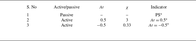
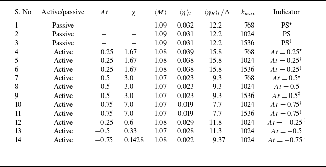


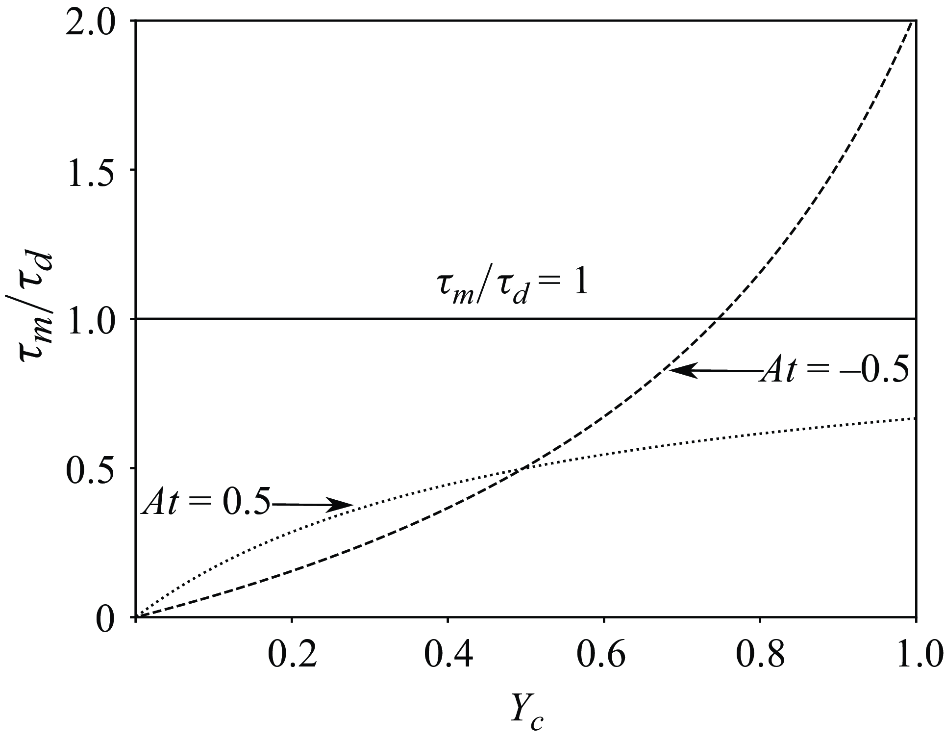

 Open access