2. Set-up and control parameters

We start with a pair of active droplets in the surfactant solution sketched in figure 1. The gradual solubilization of the oil into the surfactant micelles triggers a repulsive interaction due to the Marangoni effect (Jin et al. Reference Jin, Krüger and Maass2017). Simultaneously, the oil-filled micelles form in proximity to the droplet's surface. Additionally, we incorporate both the droplet buoyancy and the product buoyancy effects into our simulations.

Figure 1.

The set-up of the system. (a) The two droplets are initially located in the middle of the domain. The droplet buoyancy effect, the product (indicated by yellow tails under the droplets) buoyancy effect and the diffusiophoretic effect are taken into consideration. The radius of the droplets is taken as the characteristic length. The domain size expressed in this length is then $16\times 16 \times 24$. The numerical grid resolution is $161 \times 161 \times 241$. The top and bottom boundary conditions are set as a solid wall (marked by grey plane) and the boundary conditions at $x$ and $y$ directions are periodic. (b) Because of the periodic boundary condition in the $y$ direction, the two droplets in the domain align with a series of droplets. In the $x$ direction the periodic boundary condition results in a balanced force. The distance between the two neighbouring droplets inside the domain is $\ell _1$ and the distance of neighbouring particles between inside and outside of the domain is $\ell _2$.

Considering similarities between diffusiophoresis and the Marangoni effect (Desai & Michelin Reference Desai and Michelin2021), for simplicity, we focus on the phoretic effect induced by the concentration gradient of the filled micelles and will use the corresponding terminology. The physical variables describing the system are the solutal concentration $\hat {c}$ and the velocity $\hat {\boldsymbol {u}}$. Note that all dimensional physical quantities are denoted with a hat (e.g. $\hat {c}$, $\hat {\boldsymbol {u}}$).

The droplets emit solute (filled micelles) at a rate $\alpha >0$. The concentration boundary condition at the droplet surface is given by

(2.1)\begin{equation} D\frac{\partial {\hat{c}}}{\partial {\hat{n}}}={-}\alpha, \end{equation}

where $D$ is the diffusion coefficient of the dissolution product, $\alpha$ the dissolution rate at the surface and $\partial \hat {c}/\partial \hat {n}$ the concentration gradient perpendicular to the surface. The same concentration boundary condition has widely been applied in previous studies of active droplets (Hokmabad et al. Reference Hokmabad, Dey, Jalaal, Mohanty, Almukambetova, Baldwin, Lohse and Maass2021; Michelin Reference Michelin2023).

The tangential concentration gradient at the surface induces a slip velocity, known as diffusiophoretic flow. The slip velocity magnitude $u_s$ is directly proportional to the local tangential concentration gradient, given by

(2.2)\begin{equation} \hat{u}_s=M\boldsymbol{\nabla}_s{\hat{c}}, \end{equation}

where $M$ is the mobility and $\boldsymbol {\nabla }_s$ represents the tangential gradient. In our analysis, we focus on the case where $M>0$, given that the filled micelles act as a chemical repellent.

We define $\hat {\rho }_0$ as the density of the ambient fluid without any dissolved product and $\hat {\rho }_d$ as the density of the droplet itself. Note that in the experiments by Krueger et al. (Reference Krueger, Bahr, Herminghaus and Maass2016), the density difference among $\hat {\rho }_0$, $\hat {\rho }_d$ and the density of the dissolving product (filled micelles) $\hat {\rho }$ is lower than $3\,\%$. Accordingly, we adopt the Boussinesq approximation for the density difference, wherein the fluid's density $\hat {\rho }$ is assumed to be linearly proportional to the filled micelle concentration, expressed as

(2.3)\begin{equation} \hat{\rho}({\hat{c}})=\hat{\rho}_0(1+\beta \hat{c}), \end{equation}

where $\beta$ is the proportionality constant between the density and the product concentration.

The velocity field outside the droplets is governed by the Navier–Stokes equations and the product concentration field by the advection-diffusion equation. The equations are non-dimensionalized in the same way as in previous studies (Michelin, Lauga & Bartolo Reference Michelin, Lauga and Bartolo2013; Chen et al. Reference Chen, Chong, Liu, Verzicco and Lohse2021), with $R$ for lengths, $c_0=\alpha R/D$ for concentrations and $\alpha M/D$ for velocities. Note that all dimensionless quantities are represented without a hat (e.g. $c$, $\boldsymbol {u}$). The non-dimensional governing equations are presented as

(2.4)$$\begin{gather} \frac{\partial c}{\partial t}+\boldsymbol{u}\boldsymbol{\cdot}\boldsymbol{\nabla} c= \frac{1}{Pe}\nabla^2 c, \end{gather}$$

(2.5a,b)$$\begin{gather}\frac{\partial \boldsymbol{u}}{\partial t}+(\boldsymbol{u}\boldsymbol{\cdot}\boldsymbol{\nabla})\boldsymbol{u}={-}\boldsymbol{\nabla} p+\frac{Sc}{Pe}\nabla^2 \boldsymbol{u}-\frac{RaSc}{Pe^2}c\boldsymbol{e}_z,\quad \boldsymbol{\nabla} \boldsymbol{\cdot} \boldsymbol{u}=0, \end{gather}$$

and the velocity of the droplet $\boldsymbol {U}_d$ satisfies

(2.6)\begin{equation} \frac{{\rm d}\boldsymbol{U}_d}{{\rm d}t} = \frac{3Sc}{4{\rm \pi} Pe}\int (\boldsymbol{\tau} \boldsymbol{\cdot} \boldsymbol{n})\,{\rm d}S-\frac{Ga^2Sc^2}{Pe^2}\boldsymbol{e}_z, \end{equation}

where $\int (\boldsymbol{\tau} \boldsymbol{\cdot} \boldsymbol{n}) \,{\rm d}S$ is the force integrated over the surface of the droplet and $\boldsymbol {e}_z$ is the unit vector of the $z$ axis.

The dimensionless control parameters of these equations are the Rayleigh number $Ra$, which represents the strength of the product buoyancy effect,

(2.7)\begin{equation} Ra=\frac{c_0 \beta R^3 g}{\nu D} , \end{equation}

the Péclet number $Pe$, which indicates the strength of the diffusiophoretic effect,

(2.8)\begin{equation} Pe=\frac{\alpha M R}{D^2}, \end{equation}

the Schmidt number $Sc$

(2.9)\begin{equation} Sc=\frac{\nu}{D}, \end{equation}

which is kept as a constant in our study, and the Galileo number $Ga$, which represents the strength of the droplet buoyancy effect,

(2.10)\begin{equation} Ga=\frac{\sqrt{|\hat{\rho}_d/\hat{\rho}_0-1|gR^3}}{\nu}. \end{equation}

The concentration boundary condition (2.1) at the droplet surface reads in non-dimensional form

(2.11)\begin{equation} \frac{\partial {c}}{\partial {n}}={-}1. \end{equation}

The non-dimensional version of the velocity boundary condition at the droplet surface (2.2) is

(2.12)\begin{equation} u_s=\boldsymbol{\nabla}_s c. \end{equation}

We apply periodic boundary conditions along the horizontal directions ($x$ and $y$) of the domain (figure 1b), and a solid wall boundary condition at the top and bottom of the domain. The concentration and velocity boundary conditions at the top and bottom are, respectively,

(2.13)\begin{equation} \frac{\partial c}{\partial z}=0 \end{equation}

and

(2.14)\begin{equation} \boldsymbol{u}=0. \end{equation}

3. Numerical methods and validation

The Navier–Stokes equations and advection–diffusion equation are solved using direct numerical simulation in Cartesian coordinates. The spatial discretization employs a central second-order finite difference scheme. The time integration is achieved using a fractional-step method. Nonlinear terms are explicitly computed using a low-storage third-order Runge–Kutta scheme and the viscous and diffusion terms are addressed with a Crank–Nicolson scheme (Verzicco & Orlandi Reference Verzicco and Orlandi1996; Ostilla-Mónico et al. Reference Ostilla-Mónico, Yang, Van Der Poel, Lohse and Verzicco2015; van der Poel et al. Reference van der Poel, Ostilla-Mónico, Donners and Verzicco2015; Spandan et al. Reference Spandan, Lohse, de Tullio and Verzicco2018). The model for the droplet–droplet and droplet–wall collision is based on the spring-dashpot model (Costa et al. Reference Costa, Boersma, Westerweel and Breugem2015).

Because the vicinity of the surface is adopted to satisfy the constant normal fluxes and slip velocity boundary condition, we cannot allow the gap between the droplets to reach zero in collisions. Therefore, droplets are considered to be in contact when the gap width is below 2 grid spacings.

The numerical set-up is shown in figure 1. The radius $R$ of the droplet is the characteristic length of the system and the domain size is $L_x\times L_y\times L_z =16 \times 16 \times 24$. Two droplets of unit radius are initially aligned along the $y$ axis at the centre of the domain with an initial distance $L_0=4$. Uniform grids $N_x\times N_y\times N_z=161\times 161\times 241$ are employed. Since there is the periodic boundary condition along the $y$ axis, two droplets in simulations are actually a part of a series of droplets aligning along the $y$ axis. In the $x$ direction the periodic boundary conditions ensure a balanced force. We use $\ell _1(t)$ and $\ell _2(t)$ to denote the distance between the droplet and its two neighbouring droplets along the $y$ axis, and we further define $\ell (t)=\text {min}(\ell _1(t), \ell _2(t))$ as the droplet's distance to its nearest neighbour, as shown in figure 1(b).

We explore a range of parameters based on the experimental data of Krueger et al. (Reference Krueger, Bahr, Herminghaus and Maass2016): the Péclet number $0.5 \leq Pe \le 10$, Rayleigh number over the range $0.1\leq Ra\leq 245$ and the Galileo number $0 \leq Ga \le 0.19$. The Schmidt number in the experiments is of the order of $10^4$. However, the simulations at such high $Sc$ are challenging due to the very small diffusivity compared with viscosity. Therefore, in our study we set the Schmidt number to $Sc=100$.

Our code has been used to simulate diffusiophoretic particles. For the corresponding code validation, we refer the reader to our previous work (Chen et al. Reference Chen, Chong, Liu, Verzicco and Lohse2021). As a further validation, we test our code by simulating particle-laden flow incorporating both droplet buoyancy and product buoyancy effects, and compare with the existing results from the literature (Majlesara et al. Reference Majlesara, Abouali, Kamali, Ardekani and Brandt2020). The reference study considers the sedimentation of cold/hot (fixed temperature) spherical particles within a long vertical fluid channel and evaluate their terminal velocity. In that work, the product buoyancy effect is induced by the temperature variation, characterized by the Grashof number $Gr=Ra/Pr$. The particle buoyancy effect is quantified by the Reynolds number $Re$, which is linearly related to the Galileo number, $Re=\frac {2\sqrt {3}}{3}Ga$. Our code is applied to simulate the same cases as those presented by Majlesara et al. (Reference Majlesara, Abouali, Kamali, Ardekani and Brandt2020), facilitating a direct comparison of the normalized terminal velocity $U_t/U_0$ across various $Re$ and $Gr$ values, where $U_0$ is the characteristic buoyancy velocity. The numerical results are plotted in figure 2; they agree very well with those by Majlesara et al. (Reference Majlesara, Abouali, Kamali, Ardekani and Brandt2020).

Figure 2.

Code validation for a settling particle at fixed temperature in a long vertical channel. The terminal velocity $U_t$, normalized by the reference velocity $U_0$, versus the Reynolds number $Re$, which is linearly correlated to the Galileo number, $Re=\frac {2\sqrt {3}}{3}Ga$. We show results for three Grashof numbers $Gr=Ra/Pr$. The results obtained by Majlesara et al. (Reference Majlesara, Abouali, Kamali, Ardekani and Brandt2020) are indicated by filled symbols with the dashed lines. Our simulations are represented by the opened symbols, showing excellent agreement.

4. Effect of Péclet number and of Rayleigh number

In this section we first investigate the role of the Péclet number and of the Rayleigh number by simulating the interaction between a pair of droplets with $Sc=100$, $0.5 \leq Pe \leq 10$ and $0.1 \leq Ra \leq 245$. The droplet buoyancy effect is absent in this subsection ($Ga=0$) and will be analysed in § 5.

To demonstrate different interaction modes, we first focus on the cases $Pe=5$ and $Ra= 0.1$, $2$ and $245$ in figure 3, all for $Sc=100$ as throughout in this paper. For $Ra=0.1$, the diffusiophoretic effect is dominant. The mutual repulsion drives the droplets to the horizontally balanced positions ($1/4L_y$ and $3/4L_y$). The repulsion of the neighbouring droplets acts as a restoring force to the balanced position, while the droplets also experience a damping force due to the viscous drag. Therefore, the droplets perform a damped oscillation in the horizontal direction around the balanced positions. In the vertical direction the droplets rebound from the walls because of the concentration accumulation in between.

Figure 3.

Concentration contours (a–c) and distance between droplets (d–f) as a function of time for a pair of droplets in the domain with parameters $Ga=0$, $Sc=100$, $Pe=5$ and various $Ra=$ $0.1$ (a,d), $Ra=2$ (b,e), $Ra=245$ (c,f). At the right we plot the distances $\ell _1$ and $\ell _2$ defined in figure 1 as a function of time. The droplet distances corresponding to the concentration contours are indicated as red filled circles in the plots.

As $Ra$ increases to $2$, the droplets approach their neighouring droplets. The reason is that the equi-distance balanced position becomes an unstable equilibrium due to the attraction between the droplets. In the end, the two droplets reach a new balanced point of finite distance $\ell < L_y/2$. Along the vertical direction ($z$), due to the stronger product buoyancy effect, the droplets first sediment to the bottom. Then the droplets gradually float up as the concentration between the wall and the droplets accumulate. As $Ra$ further increases, the terminal distance between the neighbouring droplets decreases. For $Ra=245$, the product buoyancy effect becomes even stronger. The droplets are more attractive to each other and collide in the end.

From the results, we find that different strengths of the product buoyancy effect lead to different terminal distances between the droplets along the horizontal axis. Therefore, we define the terminal distances $\ell _\infty$ to quantify that strength:

(4.1)\begin{equation} \ell_\infty =\underset{t \to \infty}{\text{lim}} \ell(t) = \underset{t \to \infty}{\text{lim}} (\text{min}(\ell_1(t), \ell_2(t))). \end{equation}

The dependence of $\ell _\infty$ on the Rayleigh number $Ra$ is shown in figure 4(a). We identify two different types of interaction according to $\ell _\infty$. First, $Ra < 50$: without collision, where the droplets remain at an equilibrium distance without colliding with each other. The distance $\ell _\infty$ between the droplets reduces as $Ra$ increases. Second, $Ra \geq 50$, with collision, where the droplets collide due to the sufficiently strong attraction driven by the product buoyancy effect.

Figure 4.

(a) Terminal distance $\ell _\infty$ between the nearest droplets with $Ga=0$, $Sc=100$, $Pe=5$ and different $Ra$ from $0.1$ to $245$. Two interaction modes are identified, marked with different colours: $Ra \leq 50$, the droplets remain at an equilibrium distance (without collision: blue), $Ra \geq 50$, the droplets collide with each other due to the strong attraction (with collision: red). (b) The interaction modes for $Ga=0$, $Sc=100$, $0.5 \leq Pe \leq 10$, $0.1 \leq Ra \leq 245$. The blue circles represent the cases without collision, while the red triangles those with collision. The results indicate that a higher Pe results in a higher Ra threshold, above which the collision occurs.

We also simulate cases for different $Pe$ and $Ra$. The results can be classified into the two mentioned interaction modes, which are presented by different symbols in figure 4(b). From the plot, we find that a higher $Ra$ leads to collision while a higher $Pe$ leads to repulsion. The result in figure 4(b) indicates that there is competition between repulsion by diffusiophoresis and attraction by the product buoyancy effect. The two effects can be balanced, leading to the equilibrium distance for $0.5 \leq Ra \leq 50$ in figure 4(a). This complies with the experimental results of Krueger et al. (Reference Krueger, Bahr, Herminghaus and Maass2016), who found that as the surfactant concentration ($Pe$) was increased, higher density differences ($Ra$) were needed for the collective behaviour to occur.

In summary, we investigate the influence of the diffusiophoretic effect and the product buoyancy effect to the droplet interaction. Specifically, the diffusiophoretic effect (characterized by $Pe$) results in repulsion between droplets, and the product buoyancy effect (characterized by $Ra$) leads to their attraction. The mechanism of the interaction will further be quantitatively investigated in §§ 6 and 7.

5. Effect of increasing Galileo number

In this section we analyse the influence of the droplet buoyancy effect for product-buoyancy-effect-dominant cases (high $Ra$), as quantified by the Galileo number $Ga$. We numerically investigate the interactions between a pair of droplets with $Pe = 5$, $Ra = 245$ and $0 \leq Ga \leq 0.19$.

Snapshots at different times are plotted in figure 5. For all examined cases with different $Ga$, the droplets collide in the end. To further analyse the interaction, we examine the temporal change of the horizontal distance $\ell$ and the vertical height of the droplets.

Figure 5.

Concentration contours for a pair of droplets with $Sc=100$, $Pe=5$, $Ra=245$ and two different $Ga$: (a) $Ga=0.11$ (b) $Ga=0.19$.

We first plot the horizontal distance $\ell$ versus time $t$ in figure 6(a). The plot indicates that as $Ga$ increases, the waiting time for the collision to occur is longer. Next, we have a close inspection of the movement of droplets near the moment of collision through plotting $\ell -\ell _c$ as a function of $t_c - t$ in log-log scale in figure 6(b), where $\ell _c$ is the collision distance and $t_c$ is the collision time. Remarkably, all curves collapse on each other near the collision point. It suggests that the attracting behaviour of the droplets are mainly determined by $Ra$ and $Pe$, while the change of $Ga$ only leads to a delayed collision and does not influence the horizontal interaction.

Figure 6.

The plot of distance $\ell$, $\ell -\ell _c$ and height $h$ versus time $t$ or $t_c-t$ with $Sc=100$, $Pe=5$, $Ra=245$ and different $Ga$. Here $t_c$ and $\ell _c$ are the collision time and distance. (a) The distance between the two droplets $\ell$ as a function of time for different $Ga$. Subfigure (b) shows $\ell -\ell _c$ and (c) $h$ along time $t_c-t$, where $\ell _c$ is the distance at the collision point and $t_c$ is the collision time.

We also plot the height $h$ (right $y$ axis) along $t_c-t$ in figure 6(c). As $Ga$ increases, the droplets wait for longer time before the occurrence of the approaching stage, and the rising velocity is also smaller for larger $Ga$. This is because a longer time is needed to build up a sufficiently large vertical concentration gradient to lift up a heavier droplet.

In summary, based on the numerical results, we find that $Ga$ will not change the horizontal interaction between droplets, but large $Ga$ delays the collision time by reducing vertical rising velocity.

6. Attraction model with buoyancy

In this section we further investigate the origin of attraction and develop a model to estimate the attracting velocity in the buoyancy-dominant cases. Employing the point heat source model, we first derive a scaling law for the horizontal velocity around a droplet, and then calculate the attractive velocity, using the methods of reflections and Faxen's law. Since the droplet buoyancy effect only leads to delayed collision, we neglect it, i.e. we assume $Ga=0$ throughout this section.

6.1. The velocity field near a single droplet

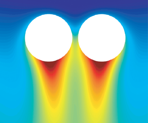
We start by simulating a single droplet to investigate the flow around it. Figure 7(a) shows the concentration and horizontal velocity ($v_y$) around a single droplet at $Ra=245$. From the fields, we observe a strong downwards plume, which leads to a higher concentration underneath the droplet. In the meantime, a horizontal flow is induced sidewards of the droplet. This inward flow drives the attraction between two nearby droplets.

Figure 7.

(a) Concentration (left half) and velocity (right half) fields near a single droplet at $Ra=245$. The streamlines are shown by the white curves. The red dashed line is at the same height as the droplet. (b) The symmetric model is plotted in cylindrical coordinates $(r, z)$ to describes the flow near the droplet with buoyancy. The buoyancy induces a strong downwards flow under the droplet and a horizontal flow near the droplet. The width of the downwards flow is $h_1$ and the horizontal one $h_2$. In the simulation we define the width $h_1, h_2$ of each flow branch by the width between $10\,\%$ of the maximum vertical and horizontal velocity.

We represent the buoyancy-driven flow near a single droplet by the schematics in figure 7(b). Since the flow around a single droplet is axisymmetric, it is illustrated in cylindrical coordinates $(r, z)$. There is horizontal inward flow sidewards of the droplet and vertical downwards flow under the droplet. In the following analysis, we will see that this horizontal inward flow is the origin of the attractive motion between nearby droplets.

A similar case that has been well studied is the natural convection near a heat source or dissolutions source (Fujii Reference Fujii1963; Moses, Zocchi & Libchaberii Reference Moses, Zocchi and Libchaberii1993; Dietrich et al. Reference Dietrich, Wildeman, Visser, Hofhuis, Kooij, Zandvliet and Lohse2016). Fujii (Reference Fujii1963) theoretically studied the buoyancy-driven convection near a fixed heat source in the fluid, and quantitatively obtained the buoyancy-driven velocity. The theoretical results were later verified in experiments with a heating sphere in a fluid by Moses et al. (Reference Moses, Zocchi and Libchaberii1993). Both the velocity and the width of the plume scale with the Rayleigh number $Ra$ (Fujii Reference Fujii1963; Moses et al. Reference Moses, Zocchi and Libchaberii1993; Dietrich et al. Reference Dietrich, Wildeman, Visser, Hofhuis, Kooij, Zandvliet and Lohse2016):

(6.1)$$\begin{gather} v_z\sim \frac{D}{R}Ra^{1/2}, \end{gather}$$

(6.2)$$\begin{gather}h/R \sim Ra^{{-}1/4}. \end{gather}$$

We define the width $h_1, h_2$ of each flow branch as the distance between $10\,\%$ of the maximum vertical and horizontal velocity. Due to the limited domain size, the vertical and horizontal flow cannot attain the asymptotic velocity of 0, preventing us from using a smaller threshold for the $h_1, h_2$ definition. The normalized values $h_1/h_1(Ra=245)$ and $h_2/h_2(Ra=245)$ vs $Ra$ for different domain sizes ($16\times 16 \times 24$ and $30\times 30 \times 24$) obtained in simulations are plotted in figure 8. When $Ra$ is large enough ($Ra \geq 100$), the width of the channel well agrees with (6.2). For $Ra < 100$, a larger domain leads to a better agreement with theory. However, there is still deviation, which attributes to the finite-size effect and the existence of a strong enough diffusiophoretic effect.

Figure 8.

The width of the downwards flow ($h_1$) and the horizontal flow ($h_2$), normalized by the corresponding height at $Ra=245$ for different $Ra$ at different domain sizes. We simulate the cases at different domain size $L_x \times L_y \times L_z =16\times 16\times 24$ denoted by $L_y=16$ and $30\times 30\times 24$ denoted by $L_y=30$. The blue and red symbols are correspondingly the numerical results for $h_1$ and $h_2$. The solid curve represents (6.2).

Given the width of both the horizontal and vertical flow, by continuity, we can further derive the relationship between the strength of the two velocities ($v_y$ for horizontal and $v_z$ for vertical), namely

(6.3) \begin{equation} v_y(r) \times 2{\rm \pi} rh_2\sim v_z \times {\rm \pi}h_1 ^2/4, \end{equation}

where $r$ refers to the horizontal distance from the droplet centre (along the red dashed curve in figure 7a). Then we define the local Reynolds number $Re_y (r)$ using the horizontal velocity $v_y (r)$. With (6.1) and (6.3), we obtain

(6.4)\begin{equation} Re_y (r)=\frac{v_y(r) R}{\nu}\sim \frac{1}{Sc} \frac{Ra^{1/4}}{r/R} . \end{equation}

We verify (6.4) with the numerical simulations of a single droplet in the domain. Note that due to the periodic boundary condition, the horizontal velocity is also influenced by the neighbouring droplets outside the domain,

(6.5)\begin{equation} \frac{Re_y (r)}{Ra^{1/4}}\sim \frac{R}{r}-\frac{R}{L_y-r}. \end{equation}

The results for different $Ra$ and $Pe$ are shown in figure 9. The numerical results agree well with the theory equation (6.5) for $r/R>4$. The results deviate near the droplet surface $r/R<4$, because the horizontal velocity reduces to zero approaching the droplet surface. A similar flow field was also observed and interpreted as a monopole component in the flow field around the active droplet by de Blois et al. (Reference de Blois, Reyssat, Michelin and Dauchot2019).

Figure 9.

Plot of $Re_y(r)$ normalized by $Ra^{1/4}$ along the red dashed line in figure 7(a) for various distances $r$ to the droplet centre normalized by the radius $R$ of the droplet. The markers are the numerical results. The solid black curve represents relationship (6.5) with a fitted prefactor $0.021 \pm 0.003$ (Everitt & Skrondal Reference Everitt and Skrondal2010).

6.2. Droplet velocity using method of reflections and Faxen's law

In this section we apply Faxen's law and the method of reflections to account for the interactions between multiple droplets. The principle of the method of reflections is to perform successive approximations for the interaction of droplets within the fluid (Guazzelli & Morris Reference Guazzelli and Morris2011; Varma, Montenegro-Johnson & Michelin Reference Varma, Montenegro-Johnson and Michelin2018). The velocity of the droplet is calculated iteratively, and in each step, the velocity of the droplet is updated with the disturbance from other droplets using Faxen's law (Guazzelli & Morris Reference Guazzelli and Morris2011). Despite the far-field assumption of the method, even for close distance $\ell /R\sim O(1)$, it reaches a surprisingly accurate result (Ishikawa et al. Reference Ishikawa, Simmonds and Pedley2006; Spagnolie & Lauga Reference Spagnolie and Lauga2012).

First, we consider a pair of active droplets (droplet 1 and 2) far apart. Since there is no external force and the droplet is isotropic, the droplets are stationary:

(6.6)\begin{equation} U_1^0=U_2^0=0. \end{equation}

Here $U_i^j$ represents the velocity of droplet $i$ after the $j$th reflection process.

Then in first reflection, we suppose that the droplets are only moderately far apart, and each droplet makes a disturbance at the velocity of the other. From (6.4), droplet 1 causes a fluid velocity disturbance at droplet 2:

(6.7)\begin{equation} u_2^0\sim \frac{D Ra^{1/4}}{\ell}. \end{equation}

Here $u_i^j$ is the fluid velocity disturbance at the centre of droplet $i$ caused by the other droplet after the $j$th reflection. According to Faxen's law, the velocity of droplet 2 due to the velocity disturbance caused by droplet 1 is (Guazzelli & Morris Reference Guazzelli and Morris2011, p. 87)

(6.8)\begin{equation} U_2^1= \left(1+\frac{R^2}{6}\nabla ^2 \right)u_2^0. \end{equation}

Since the two droplets are equivalent, the same velocity is obtained for droplet 1 after the first reflection.

Then we start with the second reflection, the velocity of the droplet obtained in the first reflection will cause disturbance to the other one. The fluid velocity caused by droplet 1 at the centre of droplet 2 is (Lamb Reference Lamb1932, p. 599)

(6.9)\begin{equation} u_2^1= \left(\frac{3R}{2\ell}-\frac{R^3}{2\ell^3} \right)U_1^1. \end{equation}

Again with Faxen's law, the velocity disturbance of droplet 2 after the second reflection is given by

(6.10)\begin{equation} U_2^2= \left(1+\frac{R^2}{6}\nabla ^2 \right)u_2^1. \end{equation}

For higher-order reflection, it is found that the velocity disturbance after reflection

(6.11)\begin{equation} U_2^n\sim O \left(\left(\frac{R}{\ell} \right)^{n-1} \right). \end{equation}

Therefore, we neglect the higher-order small terms, and the velocity of the droplet is approximated as

(6.12)\begin{equation} U(\ell)=U_2=U_2^0+U_2^1+U_2^2+O \left(\frac{R}{\ell} \right)=u_2^0+O \left(\frac{R}{\ell} \right)\sim \frac{DRa^{1/4}}{\ell}. \end{equation}

We define the Reynolds number of the droplet $Re_d$ by the droplet velocity $U$:

(6.13)\begin{equation} Re_d(\ell)=\frac{UR}{\nu}\sim\frac{D}{\nu}\frac{Ra^{1/4}}{\ell/R}=\frac{1}{Sc}\frac{Ra^{1/4}}{\ell/R}. \end{equation}

Here $Re_d (\ell )$ is different from $Re_y (r)$, where $Re_d(\ell )$ expresses the velocity of a droplet influenced by the other droplet at distance $\ell$, while $Re_y(r)$ corresponds to the fluid velocity at distance $r$ away from a single droplet.

Equation (6.13) indicates that the inward horizontal flow results in the attractive motion of a nearby droplet, but it considers the influence from only one neighbouring droplet. Note that the lateral boundaries are periodic. We consider the influence from the two neighbouring droplets and obtain

(6.14)\begin{equation} \frac{Re_d}{Ra^{1/4}}\sim \frac{R}{\ell}-\frac{R}{L_y-\ell}. \end{equation}

The equation can also be expressed as

(6.15)\begin{equation} \frac{Re_d}{Ra^{1/4}}\frac{L_y}{R}\sim \frac{1}{\ell/L_y}-\frac{1}{1-\ell/L_y}, \end{equation}

where $({Re_d}/{Ra^{1/4}})({L_y}/{R})$ is written as a function of $\ell /L_y$, facilitating the generalization of the equation to cases of different domain sizes.

6.3. Model validation

To validate the model, we calculate $({Re_d}/{Ra^{1/4}})({L_y}/{R})$ as a function $\ell /L_y$ for the droplet interaction discussed in § 4 and plot them in figure 10. The numerical results agree well with the theoretical model of (6.15). For low $Ra$ ($Ra\leq 50$), there is a deviation between the numerical results and (6.15) near the droplet, which can be explained by the influence of diffusiophoretic flow near the droplet.

Figure 10.

Plot of $Re_d(\ell )L_y$ normalized by $Ra^{1/4}R$ versus the normalized distance $\ell /L_y$ between the pair of droplets of different $Pe$, $Ra$ and domain sizes. Specifically, the case where the domain size $20 \times 20 \times 24$ is denoted by $L_y=20$, the case with a domain size of $30 \times 30 \times 24$ is indicated by $L_y=30$ and the domain size of $16 \times 16 \times 24$ is indicated without explicit reference to $L_y$. The markers are for numerical results and the black solid line for relationship (6.15) with the fitted prefactor $0.012 \pm 0.002$ (Everitt & Skrondal Reference Everitt and Skrondal2010).

To test the domain size effect of the theory, we simulate cases of domain size $20 \times 20 \times 24$ and $30 \times 30 \times 24$, and the results are also plotted in figure 10, which collapse well with theory, confirming the applicability of the theory across different domain sizes.

To further test our theory, we simulate the case of three droplets initially located at the centre of the domain with $Ra=245$, $Sc=100$ and $Pe=5$, where the snapshots are given in figure 11(a). The horizontal velocity of the middle droplet remains at zero due to the symmetry about the middle axis. With our model of § 6.2, $Re_d$ follows

(6.16)\begin{equation} \frac{Re_d}{Ra^{1/4}}\sim \frac{R}{\ell}-\frac{R}{L_y-2\ell}. \end{equation}

Indeed, in figure 11(b), for large $\ell /R$, again an excellent agreement is seen between the numerical results and the prediction of (6.16). The fitted coefficient $0.013 \pm 0.001$ is also similar to that of the case for a pair of droplets in figure 10 $0.012 \pm 0.002$, which indicates the theory is consistent for both cases. However, it is worth noting that they are different from the fitted coefficient in figure 9, because the latter case is for a different set-up: the horizontal velocity around a single droplet.

Figure 11.

(a) Snapshots at different times of concentration fields emerging from three neighbouring droplets. Here $Sc=100$, $Pe=5$ and $Ra=245$. (b) Plot of $Re_d$ normalized by $Ra^{1/4}$ versus the normalized smallest distance $\ell /R$. The symbols show the numerical results and the solid line shows relationship (6.16) with a fitted prefactor $0.013 \pm 0.001$.

7. Repulsive effect by diffusiophoresis

Given the good agreement between the attraction model with numerical results, now we further study the repulsive velocity from simulations. In the last section we found that the product buoyancy effect results in a solute convection near it, which leads to attraction between droplets. However, this solute convection also changes the flow field near the droplet, which changes the repulsive interaction due to diffusiophoretic effects. However, the concentration field with the product buoyancy effect is challenging to obtain theoretically. Therefore, in this section we analyse the repulsive effect of diffusiophoresis with numerical simulations.

We simulate a pair of droplets fixed at the centre of the domain (figure 1a) with a horizontal distance $\ell =3$ in the $y$ direction. Since the repulsive diffusiophoretic motion mainly comes from the slip velocity induced by the concentration field, we estimate the repulsive velocity by the integral of slip velocity at the surface (Stone & Samuel Reference Stone and Samuel1996):

(7.1)\begin{equation} U_{rep}=\frac{1}{4{\rm \pi} R^2}\int_S{{\boldsymbol{u}}_s\,{\rm d}S}. \end{equation}

We define $Re_{rep}=U_{rep}R/\nu$ to represent the repulsive interaction. We simulate the cases of different $Pe$ and $Ra$, and the resulting concentration field is shown in figure 12. The relationship between $Re_{rep}$ and $Pe$, $Ra$ is shown in figure 13. Figure 13(a) shows the relationship between the normalized $Re_{rep}$ and $Pe$. The results indicate that the diffusiophoretic effect leads to repulsive motion, which agrees with our conclusions in § 4, and $Re_{rep}$ is proportional to $Pe$. Figure 13(b) shows $Re_{rep}$ for different $Ra$, and we find that a stronger buoyancy effect reduces the repulsive velocity between droplets. We fit the results with a power law ansatz and get

(7.2)\begin{equation} Re_{rep}\sim PeRa^{{-}0.38}. \end{equation}

Figure 12.

The concentration field for a pair of fixed droplets at distance $3$ for $Pe=5$, $Sc=100$ and three different $Ra$ numbers: (a) $Ra=1$, (b) $Ra=10$, (c) $Ra=200$. Here $\theta$ is the angle between the bottom point and the maximum concentration point to represents the plume position.

Figure 13.

(a) Normalized droplet repulsive Reynolds number $Re_{rep}/Re_{rep}(Pe=1)$ for different $Pe$. The plot shows that the $Re_{rep}/Re_{rep}(Pe=1)$ is proportional to $Pe$. The fitting result is $Re_{rep} \sim Pe^{0.98\pm 0.03}$, which indicates a linear relationship with fitting exponent standard error $0.03$. (b) Plot of $Re_{rep}/Pe$ vs $Ra$. The solid line represents the fitted function, which shows that $Re_{rep}/Pe$ is proportional to $Ra^{-0.38 \pm 0.02}$ (Everitt & Skrondal Reference Everitt and Skrondal2010).

To better understand the decrease of $Re_{rep}$ with increasing $Ra$, we first study the influence of $Ra$ on its surrounding concentration field. We plot the concentration gradient near a single droplet of different $Ra$ at $Pe=5$ from simulations in figure 14(a). It indicates that the concentration gradient has a significant drop as $Ra$ increases. This can be rationalized as follows: as $Ra$ increases, buoyancy-driven convection reduces the thickness of the concentration boundary layer (Fujii Reference Fujii1963; Dietrich et al. Reference Dietrich, Wildeman, Visser, Hofhuis, Kooij, Zandvliet and Lohse2016). As the surface concentration gradient remains constant (2.11), a reduction in the boundary layer thickness leads to a lower local concentration gradient near the droplet.

Figure 14.

(a) Concentration gradient $|\partial c/ \partial r|$ at normalized distance $r/R$ for different $Ra$ near a single droplet, which indicates that the concentration gradient decreases as $Ra$ increases. The inset shows the normalized concentration profile. (b) The plume position $\theta$ vs $Ra$, which reflects the fact that the plume is pulled more towards the droplet bottom as $Ra$ increases.

Moreover, we find that buoyancy also influences the position of the plume at the droplet surface. Through the concentration field in figure 12, as $Ra$ increases, the plume moves closer to the bottom of the droplet. To evaluate the effect, we define $\theta$ as the angle between the maximum concentration point and the droplet bottom point to represent the position of the plume as indicated in figure 12. Figure 14(b) shows the change of the plume position for different $Ra$ at $Pe=5$. This finding thus suggests that a stronger buoyancy effect (higher $Ra$) pulls the plume towards the bottom point and this can reduce the horizontal component of the repulsive diffusiophoretic velocity.

We acknowledge that the arguments above are handwaving and qualitative. The complex system dynamics resulting from the coupling between convection and the concentration field makes a theoretical derivation of the relationship between $Re_{rep}$ and $Ra$ too challenging.

However, if we combine the equations for the attractive (6.13) and repulsive velocities (7.2), we obtain

(7.3)\begin{equation} Pe\sim Ra^{0.63}, \end{equation}

which perfectly describes the transition between the attracting and the repelling regimes; see figure 4(b). This plot nicely reflects that the mechanism behind the interaction between droplets is the competition between the attractive force by buoyancy and the repulsive force by diffusiophoresis.

9. Summary and conclusions

We have studied the interaction between droplets influenced by diffusiophoretic, droplet buoyancy and product buoyancy effects, characterized by the Péclet number ($Pe$), Galileo number ($Ga$) and Rayleigh number ($Ra$) correspondingly. We have simulated the cases over a range of $Pe$, $Ra$ and $Ga$, while keeping $Sc$ constant at $100$.

Through numerical simulations of a pair of droplets, we have found that the product buoyancy effect leads to the attractive motion between droplets, while the Marangoni/diffusiophoretic effect results in repulsion. A larger $Pe$ corresponds to a higher $Ra$ threshold for droplet collision. When $Ra$ is relatively small, the distance between droplets reaches an equi-distance equilibrium, and with increasing $Ra$, the closest balanced distance decreases, indicating that the product buoyancy weakens the Marangoni/diffusiophoretic repulsion. For sufficiently high Rayleigh numbers ($Ra\geq 50$), the droplets collide with each other. Additionally, we investigate the droplet buoyancy effect and reveal that the attracting behaviour is similar for different $Ga$, and the change of $Ga$ only leads to a delayed collision.

The simulation of a single droplet indicates that the attraction stems from convective flow induced by the density difference between the dissolving product and ambient fluid. This insight leads to a model describing the horizontal velocity near the droplet, elucidating that the local Reynolds number is inversely proportional to the distance from the droplet, as shown in (6.4).

Building on this model, we derive the equation for the attracting velocity of the droplet at high $Ra$ using Faxen's law and the method of reflections. The attracting velocity scales proportionally with $Ra^{1/4}$ and inversely with the distance between droplets. The relationship is validated through simulations involving two or three droplets.

Then we investigate the repulsive effect by simulating a pair of fixed droplets and the repulsive velocity is approximated by the integral of the slip velocity (7.1). We find that $Re_{rep}$, which represents the repulsive velocity, is proportional to $PeRa^{-0.38}$. The linear dependence of $Re_{rep}$ on $Pe$ results from a larger diffusiophoretic repulsive force for larger $Pe$, while the $Ra$ dependence indicates that higher $Ra$ leads to reduced repulsion through a reducing horizontal concentration gradient and altering plume positioning as shown in figure 14.

Combining the scaling relations of the attractive and repulsive velocity, we obtain $Pe\sim Ra^{0.63}$, aligning perfectly with the transition curve between the attractive and repulsive regime in figure 4(b). This indicates that the interplay between attractive buoyancy and repulsive diffusiophoretic forces governs droplet interaction.

We also find that for a single droplet, the sufficiently strong product buoyancy effect ($Ra \geq 0.1$) restricts the diffusiophoretic horizontal motion because the product buoyancy effect drives a downward flow near the droplet, and also drives the concentration plume closer to the bottom of the droplet, limiting the horizontal motion due to diffusiophoretic effect. This restriction also results in no discernible distinction in the interaction mechanism between low and high Péclet number with $Ra \geq 0.1$, because in both cases, the horizontal self-propulsion is restricted.

This work contributes to the understanding of the interaction between active droplets, and specifically reveals the significant role of the dissolving product buoyancy. The insights obtained clarify the attraction observed in experiments by Krueger et al. (Reference Krueger, Bahr, Herminghaus and Maass2016), and we also offer a model to predict the velocity of interacting active droplets. Our results provide a framework to understand the droplet attraction induced by the convective flow and suggest a mechanism to manipulate collective behaviours by tuning the buoyancy.

Many questions remain open. For example, how to determine the cluster size for multiple droplets? How does the flow field change if droplets are near a fluid–air interface? How to quantitatively determine the threshold Rayleigh number above which the droplets collide with each other and show collective behaviours? With the obtained insights into the attraction here, we hope it is seen as worthwhile to further explore the formation and motion of a cluster of active particles.