2.1. General framework

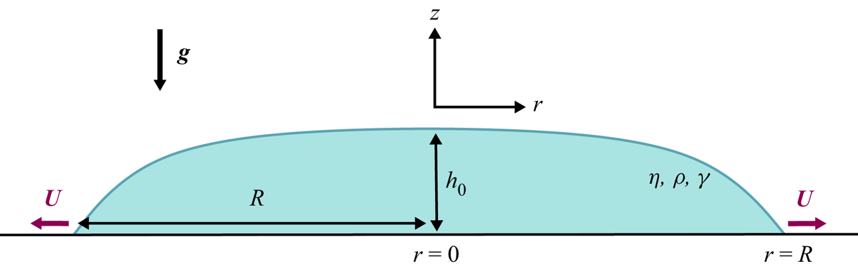
The classical situation of a fluid droplet of radius $R$ and central height $h_{0}$ that spreads onto the surface of a rigid substrate is depicted in figure 1. The fluid has dynamic viscosity $\eta$, density $\rho$, and surface tension $\gamma$. In most situations, inertia is negligible, i.e. the Reynolds number is small, $Re=\rho Uh_0/\eta \ll 1$, where $U$ is the characteristic spreading velocity. Since $h_0\ll R$, the lubrication approximation can be applied. As the flow is axisymmetric, we use cylindrical coordinates with the $z$-axis being the axis of symmetry. Under these assumptions, the height of the air–liquid interface, $h(r)$, is a solution of the free-surface thin-film equation

(2.1)\begin{equation} \frac{3\eta}{\gamma}\,\partial_{t}h+\frac{1}{r}\,\partial_{r} \left[h^2(h+3\lambda)r\,\partial_{r}\left(\partial_{rr}h+ \frac{1}{r}\,\partial_{r}h-\frac{\rho g}{\gamma}\,h \right)\right]=0, \end{equation}

where $g$ is the gravitational acceleration (Hocking Reference Hocking1981, Reference Hocking1983; Savva & Kalliadasis Reference Savva and Kalliadasis2012). A particular feature of (2.1) is that a characteristic length scale, $\lambda$, has been introduced to relax the no-slip boundary condition at the line of contact between the droplet, the substrate and the surrounding gas (Huh & Scriven Reference Huh and Scriven1971; Dussan V. & Davis Reference Dussan V. and Davis1974). In the context of the present work, we grant $\lambda$ its usual role of a slip length, and we take it to be of the order of the size of a few nanometres, comparable to that of a molecule of the liquid.

Figure 1.

Sketch of a fluid droplet spreading on a rigid substrate.

The resolution of (2.1) requires appropriate boundary conditions to be specified as

(2.2a–c)\begin{equation} h(r\rightarrow R)=0,\quad \partial_rh(r\rightarrow R)=\theta_m\quad \mbox{and}\quad \int_{r=0}^{R}h(r)\,2{\rm \pi} r\,{\rm d} r={V}_0, \end{equation}

where $V_0$ is the volume of the droplet, and $\theta _m$ is the microscopic contact angle.

Rather than providing detailed derivations of the solutions of (2.1) with these boundary conditions (2.2a–c) (see e.g. Hocking Reference Hocking1983; Cox Reference Cox1986; Savva & Kalliadasis Reference Savva and Kalliadasis2009; Sibley, Nold & Kalliadasis Reference Sibley, Nold and Kalliadasis2015), we give some insight into the different length scales involved in the problem described by (2.1) with (2.2a–c). Besides the slip length $\lambda$, we also identify the capillary length $\ell _{c}=(\gamma /\rho g)^{1/2}$, for which gravitational forces balance capillary forces, and the radius of a sphere having the same volume ${V}_0$ as that of the droplet, $R_0=(3{V}_0/4{\rm \pi} )^{1/3}$. In experiments, it usually happens that $\ell _{c}\gg \lambda$ and $R_0\gg \lambda$ by several orders of magnitude. There is thus a region in the close vicinity of the contact line in which the force balance involves only viscous and capillary forces, with slip being dominant, and gravity negligible. This viscous–capillary region will be introduced in § 2.2. On the opposite range, the large scales are governed by the balance between gravity and capillarity. This capillary–gravity region will be presented in § 2.3. In between, the three contributions of the competing viscous, capillary and gravity forces must be retained as developed in § 2.4.

2.2. Viscous–capillary region

This region corresponds to the very close vicinity of the contact line, i.e. at length scales much smaller than $\ell _c$. As mentioned earlier, in § 2.1, the introduction of a Navier slip is an important ingredient as viscous dissipation would diverge as $h\rightarrow 0$ otherwise. Resolution of the reduced equation (2.1) where the gravity term has been dropped, with the additional assumption that spreading is quasi-steady, leads to a relation often referred to as the Cox–Voinov law (Voinov Reference Voinov1976; Cox Reference Cox1986; Snoeijer Reference Snoeijer2006; Bonn et al. Reference Bonn, Eggers, Indekeu, Meunier and Rolley2009) between the velocity $U$ of the contact line and the dynamic contact angle $\theta _{app}(x)$, measured at distance $x=R-r$ from the moving rim of the droplet:

(2.3)\begin{equation} \theta_{app}^3(x)=\theta_{m}^3+9\,{Ca}\log{\left(\frac{x}{\lambda}\right)}, \end{equation}

where $Ca=\eta U/\gamma$ is the capillary number. In the case of viscous liquids, the microscopic contact angle $\theta _m$ is close to the static value (Bonn et al. Reference Bonn, Eggers, Indekeu, Meunier and Rolley2009). For (nearly) perfectly wetting liquids, it is found that $\theta _m\ll 1$ is therefore negligible in (2.3). Equation (2.3) indicates that $\theta _{app}(x)$ is an increasing function of the distance $x$ to the contact line at a given capillary number ${Ca}$. The interface in this viscous–capillary region must then have a positive curvature when measured in the frame defined in figure 1.

2.3. Capillary–gravity region

The opposite limit corresponds to the region where $r\rightarrow 0$, i.e. $x\sim R\sim R_0$. Moreover, we are interested in the limit where $R_0\gg \ell _c$. At these scales, viscous forces are insignificant and the time-derivative term in (2.1) can be dropped. In addition, in this macroscopic region, $\lambda$ can be neglected in front of $h$, which is of the order of $h_0$. Hence we are left with a capillary–gravity balance, and (2.1) reduces to

(2.4)\begin{equation} \partial_{r}\left[h^3r\,\partial_{r}\left(\partial_{rr}h+\frac{1}{r}\, \partial_{r}h-\frac{\rho g}{\gamma}\,h \right)\right]=0. \end{equation}

This equation can be integrated once. Using the boundary condition $h(r=R)=0$, the integration constant is seen to be zero. At that stage of the calculation, it is convenient to normalise the $r$ and $h$ scales as $r=R_0\tilde {r}$ and $h=h_{0}\tilde {h}$, where $R_0$ and $h_0$ are the radius of the spherical drop and the characteristic interface height in this region, respectively. Performing another integration leads to

(2.5)\begin{equation} \partial_{\tilde{r}\tilde{r}}\tilde{h}+\frac{1}{\tilde{r}}\,\partial_{\tilde{r}}\tilde{h}-{Bo}\,\tilde{h} =C, \end{equation}

where $C$ is a constant, and $Bo=\rho g R_0^2/\gamma =(R_0/\ell _c)^2$ is the Bond number of the droplet. The exact solution of (2.5) with the boundary conditions (2.2a–c) is

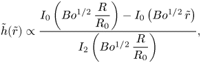(2.6)\begin{equation} \tilde{h}(\tilde{r})\propto\frac{I_0\left(Bo^{1/2}\, \dfrac{R}{R_0}\right)-I_0\left(Bo^{1/2}\,\tilde{r}\right)}{I_2\left(Bo^{1/2}\,\dfrac{R}{R_0}\right)}, \end{equation}

where $I_n(x)$ is the $n$th modified Bessel function of the first kind (Hocking Reference Hocking1983). With dimensional coordinates, the solution (2.6) reads

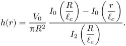(2.7)\begin{equation} h(r)=\frac{{V}_0}{{\rm \pi} R^2}\,\frac{I_0\left(\dfrac{R}{\ell_c}\right)-I_0 \left(\dfrac{r}{\ell_c}\right)}{I_2\left(\dfrac{R}{\ell_c}\right)}. \end{equation}

Droplets are spherical caps when $Bo\ll 1$, whereas their top surface flattens and they look like puddles in the limit ${Bo}\gg 1$. In the frame of reference defined in figure 1, the shape of the interface in the macroscopic region has a negative curvature.

2.4. Viscous–capillary–gravity region

We finally turn to the examination of the region for which all the contributions of the viscous, capillary and gravity forces must be kept in (2.1). In this viscous–capillary–gravity region, the length scale is comparable to neither $\lambda$ nor $R_{0}$, and the sole remaining length scale is the capillary length. Since $x, h\gg \lambda$, the reduced equation reads

(2.8)\begin{equation} 3\,{Ca}\,\partial_{r}h+\frac{1}{r}\,\partial_{rr}\left[h^3x\,\partial_{r} \left(\partial_{rr}h+\frac{1}{r}\,\partial_{r}h-\frac{h}{\ell_{c}^2}\right)\right]=0, \end{equation}

where we consider quasi-static spreading and use $\partial _{t}h=U\,\partial _{r}h$. This assumption means that at any time, the velocity of the contact line sets the drop shape with no transient involved. This constraint is enforced by the hypothesis that $Re\ll 1$ (Gratton et al. Reference Gratton, Diez, Thomas, Marino and Betelú1996). The capillary number $Ca=\eta U/\gamma$ then appears as a natural way to build a dimensionless velocity.

As mentioned above, the capillary length $\ell _c$ is the only length available. It is the scale for the variation along the horizontal direction, $r=\ell _{c}\hat {r}$. However, no obvious length scale emerges in the vertical direction. We thus define $h=h^\star \hat {h}$, where $h^\star$ is the (still unknown) relevant scale for the drop height. Using these renormalisations in (2.8) yields

(2.9)\begin{equation} 3\,Ca\,\partial_{\hat{r}}\hat{h}+\left(\frac{h^\star}{\ell_{c}}\right)^3 \frac{1}{\hat{r}}\,\partial_{\hat{r}}\left[\hat{h}^3\hat{r}\,\partial_{\hat{r}} \left(\partial_{\hat{r}\hat{r}}\hat{h}+\frac{1}{\hat{r}}\,\partial_{\hat{r}}\hat{h}-\hat{h} \right)\right]=0. \end{equation}

For the two terms to be of the same order in (2.9), one must take the height scale to be

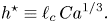(2.10)\begin{equation} h^{{\star}}\equiv\ell_{c}\,Ca^{1/3}. \end{equation}

This scale represents the typical height separating the viscous–capillary region governed by the Cox–Voinov law from the viscous–capillary–gravity region where gravity comes into play in the force balance. In other words, this transition scale corresponds to the upper bound of the region of the drop where the Cox–Voinov relation (2.3) is still valid. Another interesting interpretation of $h^\star$ is that it may delineate the change in surface curvature and thus can be understood as the inflection point of the drop interface.

Some orders of magnitude can be provided for the present experimental conditions. The range of $h^\star$ is $20\leq h^\star \leq 800\,\mathrm {\mu }$m for typically $\ell _c\simeq 2$ mm and $10^{-6}\leq Ca\leq 10^{-2}$. As a consequence, liquids with sub-millimetre characteristic length scales, such as suspensions of non-Brownian particles, may show non-trivial $\theta _{app}\unicode{x2013}Ca$ relations. Indeed, adding density-matched particles should not modify the drop behaviour in the gravity-driven region, while it should enhance dissipation provided that the particles can access the region where viscosity matters, namely the dissipation region for $h\lesssim h^\star$.

3.1. Particles and fluid

The suspending fluid is a Newtonian PEG copolymer, poly(ethylene glycol-ran-propylene glycol) monobutyl ether (average $M_n\simeq 3900$, Sigma-Aldrich reference 438189), with a density close to that of polystyrene, $\rho =1056$ kg m$^{-3}$, at temperature $25\,^{\circ }$C. Its dynamic viscosity $\eta _f=2.4\pm 0.1$ Pa s is constant over a large range of shear rate (0.01–10 s$^{-1}$) at $25\,^{\circ }$C. Particles are spherical polystyrene beads (Dynoseeds TS, Microbeads, Norway) that are sieved when necessary to remove small dust particles or to narrow the size distribution below a tenth of particle diameter. The mean particle diameters $d$ used in the experiment are 10, 20, 40, 80, 140 and $250\,\mathrm {\mu }$m. Density-matching between the liquid and the particles is sufficient to prevent buoyancy effects over hours at temperature $25\,^{\circ }$C in the air-conditioned room. To prepare the suspension mixture, the suspending fluid is weighted and poured into a test tube. A desired mass of particles is then added to reach the target volume fraction $\phi$. Good mixing while avoiding entrapping of air is achieved by hand mixing followed by slow mixing on a rolling device overnight. In the following experiments, the solid volume fraction is $\phi =0.4$ as we aim to study the strongest effects expected at large volume fractions (Zhao et al. Reference Zhao, Oléron, Pelosse, Limat, Guazzelli and Roché2020). The particle surface is completely wet by the suspending fluid, i.e. particles remain suspended in the fluids and do not aggregate. We measured the surface tension of the suspension using pendant drop experiments. We find that the suspension surface tension is equal to the surface tension of the suspending fluid, $\gamma =\gamma _f\simeq 35\,{\rm mN}\,{\rm m}^{-1}$, a similar result to that reported in Couturier et al. (Reference Couturier, Boyer, Pouliquen and Guazzelli2011).

3.2. Bulk suspension rheology

A thorough discussion of our results requires a comparison of the bulk viscosity of the granular suspensions with their apparent viscosity extracted from drop spreading experiments; see § 5. Rheological measurements have been performed using an ARES G2 rheometer (TA Instruments) with a 25 mm-wide plate–plate geometry for solid blends of moderate-size particles with diameters 10, 20, 40 and $80\,\mathrm {\mu }$m. The thickness of the gap between the plates is typically $1.5$ mm, i.e. at least 20 particle diameters, to prevent confinement effects (Peyla & Verdier Reference Peyla and Verdier2011). As wall-slip effects depend on the gap thickness, the fact that no viscosity variation is measured while changing the gap thickness from 1 to 2 mm indicates that sliding is negligible for these small particles (Yoshimura & Prud'homme Reference Yoshimura and Prud'homme1988; Jana, Kapoor & Acrivos Reference Jana, Kapoor and Acrivos1995).

Confinement and slip become important when performing rheological measurements with suspensions of particles with diameters of 140 or $250\,\mathrm {\mu }$m. Slip is avoided using a 25 mm-wide plate–plate cross-hatched geometry with typical roughness 1 mm. Confinement is a trickier issue since increasing the gap thickness leads to a larger meniscus and thus to a significant error in viscosity measurements (Cardinaels, Reddy & Clasen Reference Cardinaels, Reddy and Clasen2019). We circumvent this issue by using a wide reservoir (a 5 cm-wide cup) mounted on the lower plate and filled with a 5 mm-thick layer of suspension (${\gtrsim }20d_p$) on which the upper tool is lowered to touch the free interface (Château et al. Reference Château, Guazzelli and Lhuissier2018; Château & Lhuissier Reference Château and Lhuissier2019). The additional torque exerted by the exceeding fluid in the reservoir can be computed analytically if the reservoir width and the suspension thickness are known (Vrentas, Venerus & Vrentas Reference Vrentas, Venerus and Vrentas1991). We have implemented this correction numerically, and we have been able to reproduce both published data and experimental results with and without the reservoir for Newtonian fluids and dense suspensions of 80 $\mathrm {\mu }$m particles.

The relative bulk viscosity of monomodal granular suspensions, $\eta _s$, is defined as the viscosity of the whole suspension relative to that of the viscosity of the suspending fluid. It is independent of the particle size and shear rate, and is solely an increasing function of the particle volume fraction $\phi$ that diverges at a maximum value $\phi _c$ for which the suspension ceases to flow as shown in figure 2(a). Note that the value $\phi _c\simeq 0.53$ inferred from curve fitting is provided for the plot, but a more exhaustive study of the viscosity in the dense regime would be required to confirm this value. The value of $\phi _c$ depends on the frictional contacts between particles (see e.g. Tapia, Pouliquen & Guazzelli Reference Tapia, Pouliquen and Guazzelli2019). It is important to note for the following discussion that $\phi _c$ also depends on the particle-size distribution for polydisperse suspensions.

Figure 2.

Relative viscosity (i.e. shear viscosity of the suspension relative to that of the suspending fluid) $\eta _s$ of (a) monomodal and (b) bimodal suspensions averaged for shear rates between 0.1 and 1 s$^{-1}$ corresponding to the range of shear rates of the spreading experiments. (a) Relative viscosity of monomodal suspensions as a function of particle volume fraction $\phi$ for particles with diameters 10, 20, 40, 80, 140, $250\,\mathrm {\mu }$m and comparison with experimental data for particles with diameters $10$ and $140\,\mathrm {\mu }$m from the experiments of Château, Guazzelli & Lhuissier (Reference Château, Guazzelli and Lhuissier2018) and Palma & Lhuissier (Reference Palma and Lhuissier2019), respectively. The vertical dotted line is an estimate of the maximum volume fraction $\phi _c\simeq 0.53$ used to compare data with the empirical correlations of Krieger & Dougherty (Reference Krieger and Dougherty1959), $\eta _s=(1-\phi /\phi _c)^{-[\eta ]\phi _c}$, and Eilers (Reference Eilers1941), $\eta _s=(1+[\eta ]/2\phi /(1-\phi /\phi _c))^2$ (where $[\eta ]=2.5$ is the intrinsic viscosity of the suspension). (b) Relative viscosity of bimodal suspensions at a fixed total solid volume fraction $\phi =0.4$ as a function of the fraction of the small particles in the solid phase, $\zeta _{small}$, for two-size blends (see legend).

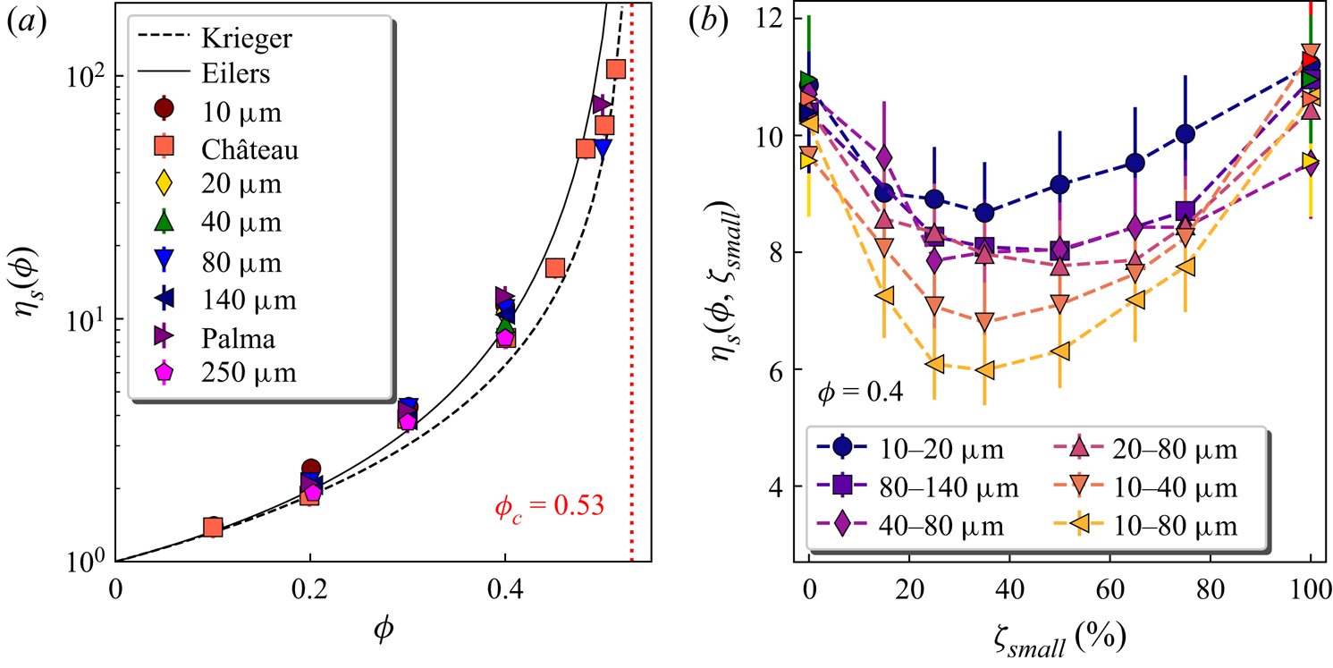
For bimodal suspensions, the viscosity depends not only on $\phi$ but also on the particle sizes $d_1$ and $d_2$ ($d_1< d_2$) of the two species, and on the fraction of small particles in the solid phase, $\zeta _{small}$; see figure 2(b). Experimental studies of dense bimodal systems in the literature indicate that their viscosity is also controlled by the value of the maximum packing fraction $\phi _c$, which is found to be higher than that of monomodal suspensions (Chong, Christiansen & Baer Reference Chong, Christiansen and Baer1971; Chang & Powell Reference Chang and Powell1994). This increase in $\phi _c$ results from the ability of small particles to fill the holes between the large ones (Macosko Reference Macosko1994). For bimodal suspensions with a given size ratio $d_2/d_1$, the relative bulk viscosity $\eta _s$ is equal to that obtained in the sole presence of the large particles, when $\zeta _{small}=0\,\%$. Increasing $\zeta _{small}$ leads to a decrease of $\eta _s$, down to a minimum located between $\zeta _{small}=25\,\%$ and $\zeta _{small}=50\,\%$, and then to an increase up to the value obtained for a suspension of small particles, $\zeta _{small}=100\,\%$. The minimum in viscosity is more pronounced with increasing $d_2/d_1$; see figure 2(b).

3.3. Experimental apparatus

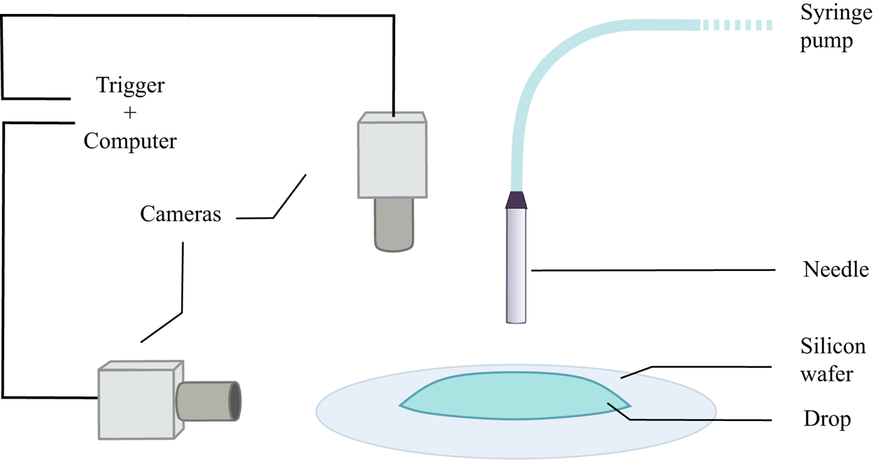
We create droplets of suspension having volume $V_0= 300\,\mathrm {\mu }$l (spherical radius ${R_0=4.15}$ mm) with a syringe pump (flow rate 10 ml min$^{-1}$), as shown in figure 3. The droplets spread over a silicon wafer (Si-Mat) cleaned with ethanol and distilled water, and dried with clean-room wipes (plasma cleaning did not change the results or the quality of the data and was therefore considered an unnecessary precaution). Acquisition is made from side and top views with two synchronised monochrome cameras (Basler acA2440-35um, $2000\times 2448$ pixels) on which 1 : 1 macro objectives are mounted (I2S visions, MC series). High spatial resolution is required to capture the dynamics of the contact line. These optics give resolution $3.45\,\mathrm {\mu }$m px$^{-1}$. Frame rates from 5 to 10 f.p.s. are required for the side view, especially at the beginning as the drop spreads quickly. Frame rates of 0.5 f.p.s. are sufficient for the top view as most of the interesting data are extracted at long times when spreading is slow and the slope of the drop interface is not too steep. A typical set of experiments for a single suspension batch is made of 10 different runs of spreading drops. These runs are acquired after 10 unused runs (corresponding to a total amount $\sim$3 ml) to avoid effects coming from the front of the advancing suspension in the tubing and in the needle. After performing these blank runs, the experiments are seen to be very reproducible at the desired volume fraction $\phi =0.4$. Care is also taken to account for temperature and humidity variations. These two factors impact mainly the suspending fluid viscosity $\eta _f$. To this end, systematic viscosity measurements are performed during the experiments using a capillary viscometer.

Figure 3.

Sketch of the experimental apparatus.

3.4. Side-view analysis

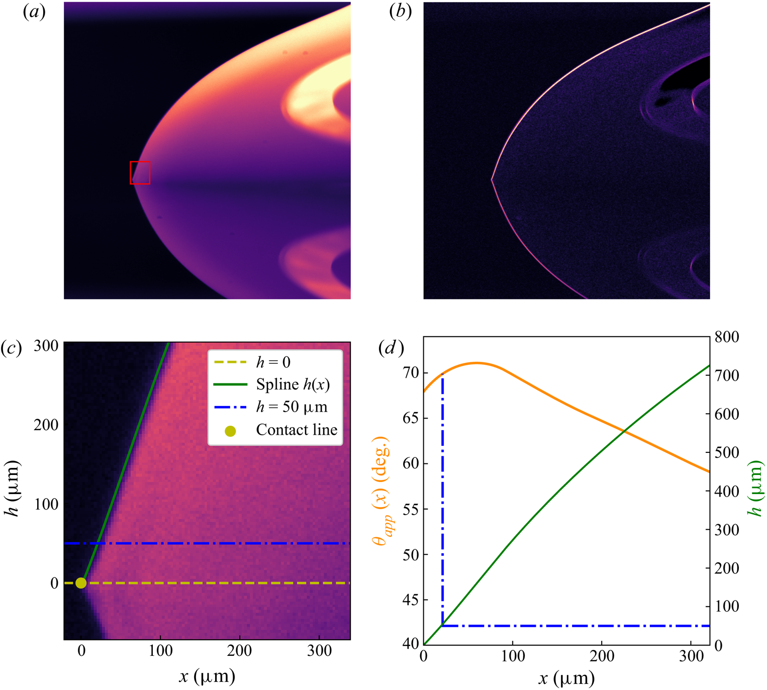
We characterise the dynamics of spreading by measuring the dynamic contact angle $\theta _{app}$ as a function of the dimensionless contact line velocity $U$. Angle measurement from the side views has been improved from the previous work of Zhao et al. (Reference Zhao, Oléron, Pelosse, Limat, Guazzelli and Roché2020) owing to better optical resolution and the possibility of performing an automated local angle measurement. We tailor the background lighting of our system with masks so that the drops captured by the side camera appear bright on a dark background, as seen on the top part of figure 4(a). Drop-shape detection is performed with the Sobel filter of the scikit-image package in Python, shown in figure 4(b), and further thresholded to extract the contact line coordinates and the drop profile $h(x)$, with $x=0$ being the position of the contact line; see figure 4(c). The position of the contact line is defined as the leftmost bright pixel after image processing, as presented in figures 4(b,c). The drop profile is then smoothed with a cubic spline, as shown in figures 4(c,d). The contact line velocity $U$ is obtained by locating the triple contact line, while the apparent dynamic contact angle $\theta _{app}$ is inferred from the derivation of this spline. A spline is a piecewise polynomial function defined by the number of points, or knots, that it passes through. Spline functions are regular at zero, first and second order of derivation, as demonstrated in figure 4(d). To optimise spline adjustment to the data at all slopes, a small knot-to-knot distance is chosen at early times and then increased as the drop flattens. This process prevents meaningless oscillations at small slopes (large distance between knots). For all pictures, improper fits due to loss of focus or dust are discarded. The results are found to be similar to those obtained by adjusting manually a straight line to the air/liquid interface near the contact line in the range $30^{\circ } \lesssim \theta _{app}\lesssim 85^{\circ }$. The fitted profile can then be derived once or twice at any point of the interface. The possibility of changing the measurement height $h$ of the contact angle is one of the major benefits of this automated numerical procedure compared to previous manual measurements; see figure 4(d).

Figure 4.

Data extraction from a picture of a spreading drop. Reflection on the wafer helps to detect the advancing contact line: (a) raw picture, and (b) Sobel filtering. The red rectangle in (a) corresponds to the blown-up region in (c), showing the fitted spline of the drop profile (green curve), the position of the contact line (yellow dot), and the drop height $h=50\,\mathrm {\mu }$m (dash-dotted blue line). (d) Results extracted from the fit: drop height $h$ as a function of the distance to the contact line $x$ (green), and contact angle computed from the spline derivation according to $\theta _{app}(x)=\tan ^{-1}({{\rm d}h}/{{\rm d}\kern0.7pt x})$ (orange).

3.5. Top-view analysis

Top views are used to visualise the structure of the particle network near the contact line, and also to measure the distance between the particles and the contact line $L$. Measurements using the ImageJ FiJi software package (Schindelin et al. Reference Schindelin2012) are performed over roughly 30 particles at the front. The precision of these measurements is set by the resolution of the pictures ($3.45\,\mathrm {\mu }$m px$^{-1}$).

4.1. Simple fluids

In § 2.4, we have identified the length scale $h^\star$ that characterises the height of the interface at the transition between the viscous–capillary regime governed by the Cox–Voinov relation (2.3) and the viscous–capillary–gravity regime where gravity starts to prevail and where an inflection point should exist. We start our experimental characterisation of $h^\star$ by investigating the shape of the interface in the case of simple fluids.

Inspired by the form of the Cox–Voinov law (2.3), we measure, for capillary numbers in the range $0.0025\leq Ca\leq 0.0125$, how the cube of the angle between the interface and the horizontal, $\theta _{app}^3$, depends on the interface height $h$ and on the horizontal distance to the contact line $x$; see figures 5(a,b), respectively. The data come from the average over 7 experimental runs. We identify two regions. Starting from the contact line, for any capillary number, $\theta _{app}^3$ is first independent of the height at which it is measured; see figure 5(a). A plateau can thus be defined for $h$ ranging from 10 to almost $100\,\mathrm {\mu }$m. Note that this plateau is better seen in semi-log scale in figure 5(a). Discussion of these results in the light of the Cox–Voinov law would lead us to expect that $\theta _{app}^3$ is an increasing function of $h$. However, two experimental facts may prevent us from seeing this increase. First, an inflection point can be seen for some experiments (see, for instance, figure 4d), but the process of averaging over several runs likely smears out the change of curvature. Second, the length scales that we can probe are at least three orders of magnitude larger than the nanometric cut-off scale $\lambda$. We thus expect the logarithmic term to increase slowly with distance, leading to difficulties in distinguishing the shape of the interface from a straight line. Similar conclusions regarding the local slope near the contact line have been reached by Rio (Reference Rio2005). It is worth mentioning that the plateau value increases with the capillary number as expected from the Cox–Voinov law (2.3). Away from the contact line, the angle decreases, suggesting a growing contribution of gravity to the force balance. In figure 5(b), the experimental contact angle is plotted, and the theoretical prediction obtained from the balance between gravity and capillarity is superimposed at largest distances from the contact line. We find that the agreement of the static solution (2.7) with the data is satisfactory and improves with decreasing $Ca$, provided that we leave the radius of the droplet as a fitting parameter since it cannot be inferred in our experiments. Indeed, the imaging field does not cover the whole drop as the focus is on the contact line region, which requires a significant magnification.

Figure 5.

Cube of the contact angle $\theta _{app}^3$ versus (a) the measurement height $h$, and (b) the horizontal distance to the contact line $x$, averaged over 7 experimental runs for 5 capillary numbers $Ca$, namely 0.0025 ($\lozenge$), 0.005 ($\circ$), 0.0075 ($\triangle$), 0.01 ($\square$), 0.0125 (), using a Newtonian fluid (PEG copolymer). Red dashed lines indicate static shape (2.7) for $R=8.5,8.7,8.9,9.3, 10$ mm (estimated so as to provide the best fit with the experimental data) and $\ell _c=1.82$ mm. (c) Normalised cube of the contact angle $\theta _{app}^3/\theta _{app}^3(h\rightarrow 0)$ versus normalised height $h/\ell _c$. Black dotted line indicates the threshold for the plateau length at $\theta ^3(h^\star )/\theta ^3(h\rightarrow 0)=0.9$. (d) Normalised transition height $h^\star /\ell _c$ versus $Ca$ for three different Newtonian fluids: PEG (black $\lozenge$), silicone oil V1000 (maroon $\square$; $\rho =970$ kg m$^{-3}$, $\gamma =21$ mN m$^{-1}$, $\eta =1.0$ Pa s, $\ell _c=1.46$ mm), and glycerol (red ; $\rho =1260$ kg m$^{-3}$, $\gamma =63$ mN m$^{-1}$, $\eta =1.3$ Pa s, $\ell _c=2.23$ mm), as well as the inflection-point measurements (gold $\circ$) of Tanner (Reference Tanner1986) with highly viscous silicone oil. Black solid line indicates $h^\star /\ell _c=0.3\,Ca^{1/3}$.

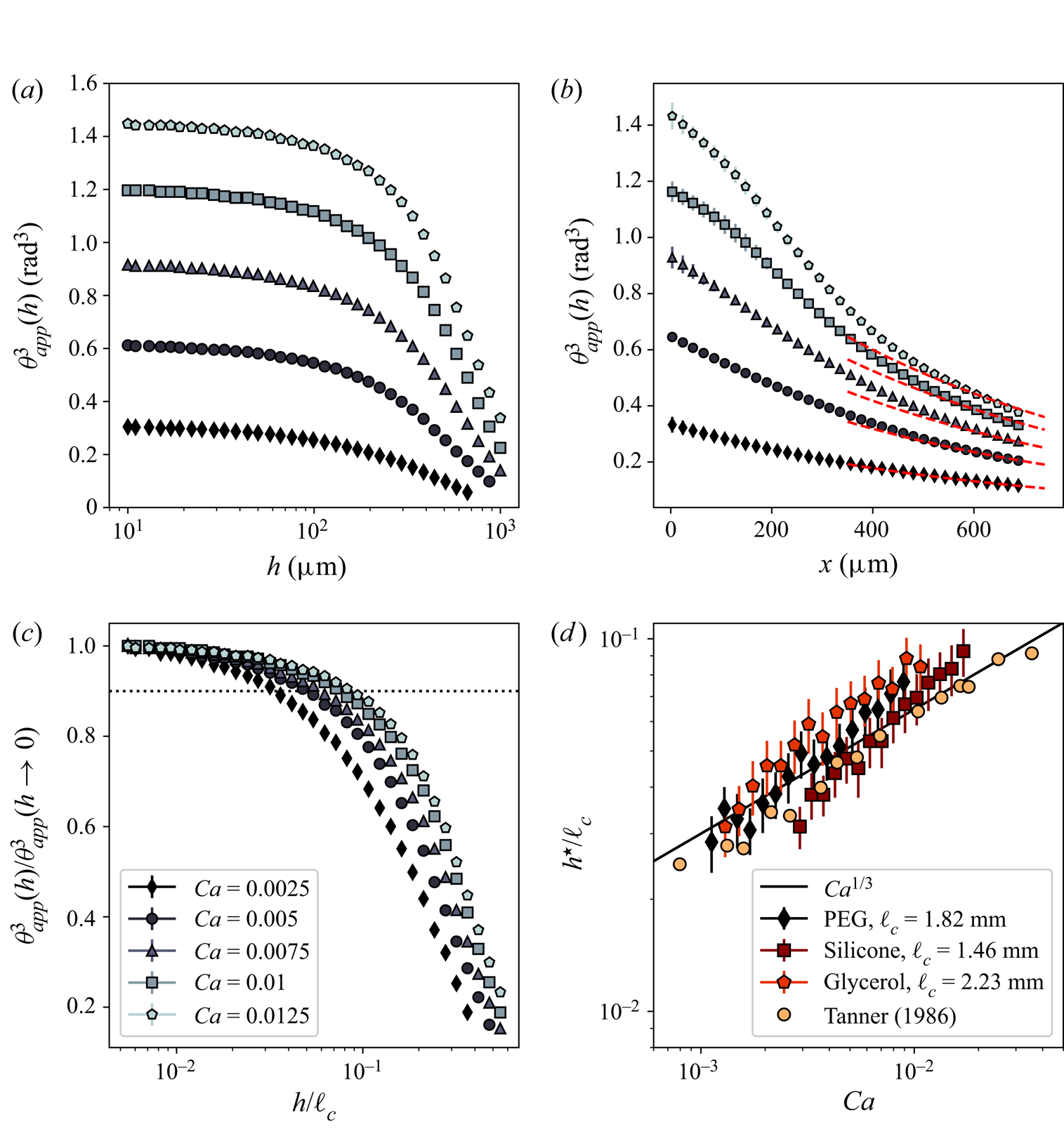
Comparison of the datasets is made easier if we normalise $\theta _{app}^3(h)$ by its asymptotic value $\theta _{app}^3(h\rightarrow 0)$, and $h$ by the capillary length $\ell _c$; see figure 5(c). From these plots, we define the experimental transition height $h^\star$ as the height at which $\theta _{app}^3(h)$ departs from $\theta _{app}^3(h\rightarrow 0)$ by 10 %. Figure 5(d) shows the inferred $h^\star$ as a function of $Ca$ for different simple fluids. The normalised transition height $h^\star /\ell _c$ increases as $Ca^{1/3}$ in agreement with the prediction (2.10) of the dimensional analysis in § 2.4. We also report in this graph the measurements of the inflection point of the interface obtained by Tanner (Reference Tanner1986), although the present interpretation as an upper limit of dissipation was not mentioned in this work. These data agree well with the present estimates of $h^\star$ as well as with the $Ca^{1/3}$ scaling. Note that this scaling still holds when varying the threshold between 1 % and 15 %. The threshold of 10 % provides the best match with the measurements of Tanner (Reference Tanner1986). If we grant $h^\star$ the interpretation of a viscous–capillary cut-off length and refer to figure 5(d), then we can conclude that measuring contact angles at heights well below $100\,\mathrm {\mu }$m warrants probing the region of the droplet where the apparent dynamic contact angle is set by a balance between viscous dissipation and capillarity only.

4.2. Granular suspensions

We now test the relevance of $h^\star$ to the spreading of drops of granular suspensions. Because they are density-matched to the suspending fluid and do not modify surface tension, the particles are expected to modify only viscous dissipation and to leave gravitational and capillary effects unchanged.

Figure 6(a) presents the variation of $\theta _{app}^3$ with the measurement height $h$ for monomodal granular suspensions of 10 $\mathrm {\mu }$m particles and bimodal suspensions of 10–80 $\mathrm {\mu }$m particles with $\zeta _{10}=50\,\%$, at a constant capillary number $Ca_0=\eta _f U/\gamma _f$, where subscript $0$ on the capillary number emphasises that it is computed using properties of the suspending fluid. Reference data for the pure suspending fluid at $Ca_0$ are also provided for comparison in figure 6(a). The behaviour of $\theta _{app}^3(h)$ for the suspensions is similar to that seen for the reference fluid; see also figures 5(a,c). A plateau region is again observed close to the contact line, for $10\lesssim h\lesssim 100\,\mathrm {\mu }$m, while there is a decay at larger distances. The addition of the particles leads to an increase in the plateau value of $\theta _{app}^3$, which depends on the particle mixture components. Provided that measurements are undertaken within the plateau region at constant height across all experiments, we can obtain an unequivocal apparent contact angle, at a given capillary number. The dependence between these two quantities is then a priori interpretable in terms of the Cox–Voinov relation. In the following, the measurement height is set at $h=50\,\mathrm {\mu }$m. This chosen height seems a good compromise between smaller heights having large measurement noise and larger heights that might fall outside of the region where viscosity matters. Note that taking $h$ in the range 20 to $100\,\mathrm {\mu }$m yields similar results for the apparent wetting viscosity that will be introduced below.

Figure 6.

(a) Cube of the contact angle $\theta _{app}^3$ versus the measurement height $h$ for different fluids: pure suspending fluid (grey $\triangle$), 10 $\mathrm {\mu }$m monomodal suspension (red $\square$), and 10–80 $\mathrm {\mu }$m bimodal suspension at $\zeta _{10}=50\,\%$ (orange $\circ$), resulting from the analysis of 7, 8 and 10 drop-spreading runs, respectively, and at the same fluid capillary number $Ca_0=\eta _f U/\gamma _f=0.0025$. Inset: normalised cube of the contact angle $\theta _{app}^3/\theta _{app}^3(h\rightarrow 0)$ versus normalised height $h/\ell _c$. Blue dash-dotted line indicates selected measurement height $h=50\,\mathrm {\mu }$m. (b) Variation of $\theta _{app}^3/9$ as a function of $Ca_0$ performed at height $h=50\,\mathrm {\mu }$m for the different runs for spreading drops made of pure suspending fluid (grey dots), 10 $\mathrm {\mu }$m monomodal suspension (red dots), and 10–80 $\mathrm {\mu }$m bimodal suspensions at $\zeta _{10}=50\,\%$ (orange dots). The different colour shades represent different experiments. The dashed lines correspond to the average of the linear fits of data coming from each run and are used to infer the relative apparent viscosity $\eta _w$.

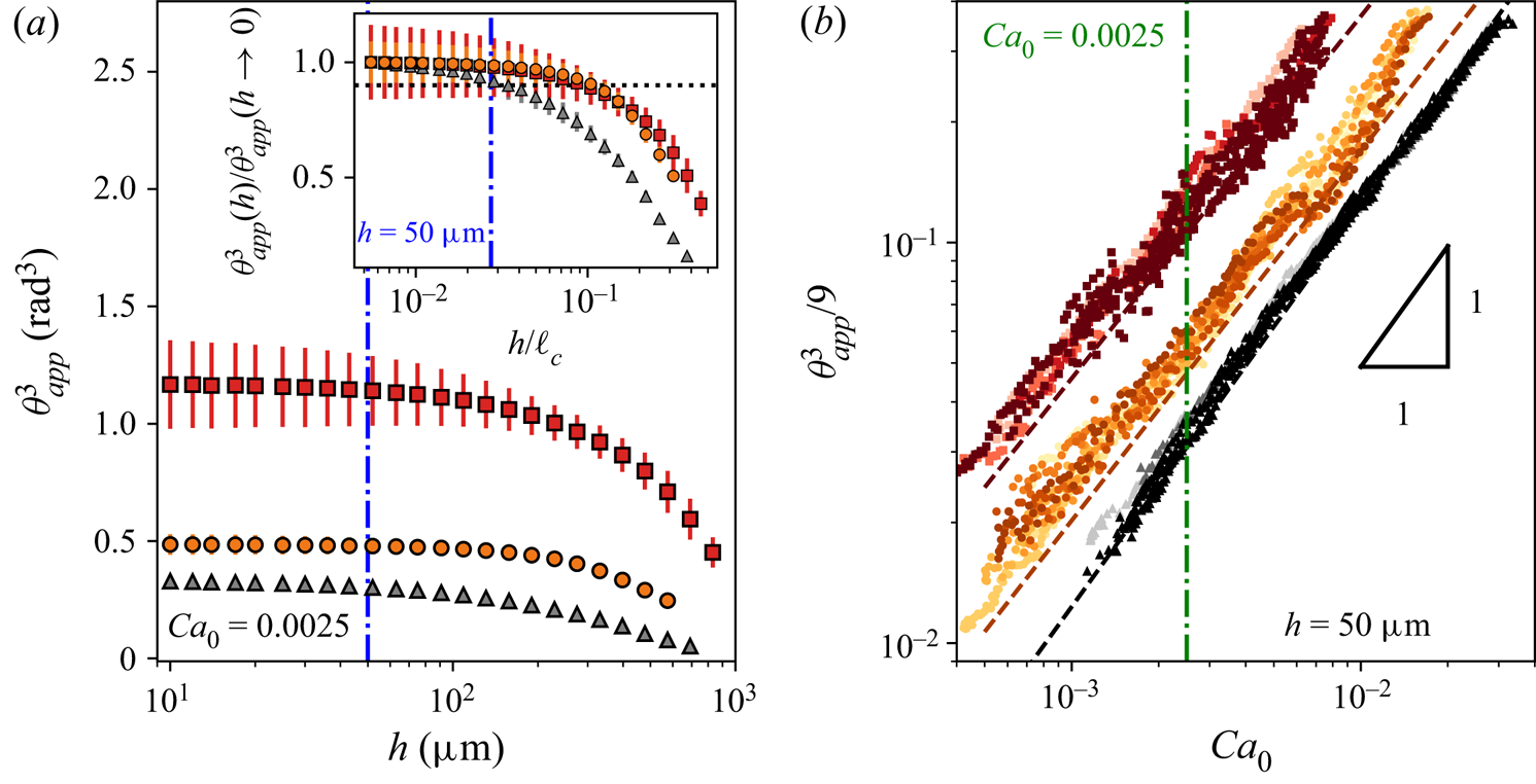
Figure 6(b) displays typical variations of $\theta _{app}^3/9$ as a function of the capillary number of the suspending fluid, $Ca_0$. Data from different experimental runs are plotted for the same fluids as those used in figure 6(a). For a given fluid (suspensions or reference fluid), the tight collapse of the different $\theta _{app}^3(Ca_0)$ curves coming from the different runs bears witness to the good reproducibility of the experiments. All the datasets collapse on straight lines with unity slopes in log-log representation, i.e. $\theta _{app}^3/9\propto Ca_0$. For each run, a linear fit is performed and the average (dashed) line for a given fluid is the average of the corresponding linear fits. Typically, the measured angles lie between 30$^{\circ }$ and 90$^{\circ }$, the upper limit being set by the algorithm. Tracking is interrupted below 30$^{\circ }$ due to the failure of the Cox–Voinov law. Protrusions of the particles from the free surface are observed at small contact angles and might be responsible for this discrepancy.

As expected, the data from the suspending fluid are in excellent agreement with the Cox–Voinov law (2.3). The logarithm factor in (2.3) is found to be ${\simeq }11.9$, in good agreement with values in the literature (Voinov Reference Voinov1976). It is important to note that the measurements are undertaken at a constant height $h$ within the plateau region, and not at a constant $x$. However, since $x$ and $h$ are of the same order of magnitude and sufficiently large compared to $\lambda$, the logarithm factor is not varying significantly and can be considered constant.

For suspensions, data for $\theta _{app}^3(Ca_0)$ in figure 6(b) equally collapse on a straight line with a slope of unity in the log-log representation (red and orange dashed lines): the spreading of these materials still seems to follow a Cox–Voinov relation (2.3). However, since the values of $\theta _{app}^3$ in the plateau are changed by the addition of particles as shown in figure 6(a), the different $\theta _{app}^3(Ca_0)$ lines are shifted with respect to each other in figure 6(b), in agreement with previous experiments (Zhao et al. Reference Zhao, Oléron, Pelosse, Limat, Guazzelli and Roché2020). Assuming that the logarithmic factor has the same order of magnitude for the pure suspending fluid and for suspensions (as we do not expect the particles to modify the mechanics at the nanometric scale), we can superimpose all curves and recover the Cox–Voinov law (2.3) for all liquids if we adjust the viscosity used in the capillary number $Ca=\eta U/\gamma$, with $\eta =\eta _f\eta _w$ where $\eta _w$ is the relative apparent wetting viscosity of the suspensions. Again, the shift and consequently the apparent wetting viscosity strongly depend on the particle mixture components. Here, we see that the suspension of 10 $\mathrm {\mu }$m particles has a larger apparent wetting viscosity than the 10–80 $\mathrm {\mu }$m bimodal suspension. The behaviour of the apparent viscosity $\eta _w$ is examined in detail in § 5 for suspensions consisting of different particle combinations.

5.1. Suspensions with particles having a large difference in size

We focus first on suspensions consisting of particles having a large difference in diameter, $d_1=10\,\mathrm {\mu }$m and $d_2=80\,\mathrm {\mu }$m ($d_2/d_1=8$). Figure 7(a) shows that the relative wetting viscosity of these suspensions, $\eta _w$, increases with increasing fraction of the small particles, $\zeta _{10}$, with a steeper growth beyond $\zeta _{10} \simeq 50\,\%$. This behaviour is in stark contrast with the $\zeta _{10}$ dependence of the relative bulk viscosity of the same mixtures shown in figure 2(b) and plotted again in the inset in figure 7(a). The relative bulk viscosity of the blends presents a minimum at $\zeta _{10}=35\,\%$, i.e. a mixture containing roughly a third of small particles. This minimum viscosity is 40 % smaller than the values obtained in the monomodal cases at $\zeta _{10}=0\,\%$ and 100 % (consisting of monomodal suspensions of 80 and $10\,\mathrm {\mu }$m, respectively). It is worth noting that even in the monomodal case with the small particles, $\eta _w$ is smaller (by a factor of order 2) than the corresponding value of its bulk viscosity, $\eta _s$. This inability to reach the bulk value is always observed even for the smallest particles as there is always a small region devoid of particles at the tip followed by an ordered region, as discussed in the following and in § 6.

Figure 7.

Experimental results for suspension blends with fixed $d_1=10\,\mathrm {\mu }$m and $d_2=80\,\mathrm {\mu }$m, and varying $\zeta _{10}$ at $\phi =0.4$. (a) Relative wetting viscosity $\eta _w$ as a function of the fraction of the small particles in the solid phase, $\zeta _{10}$. Inset: bulk viscosity $\eta _s$ of the corresponding suspensions versus $\zeta _{10}$. The dotted lines are guides for the eyes. (b) Top-view pictures taken when $\theta _{app}=35^{\circ }$ at $h=50\,\mathrm {\mu }$m for $\zeta _{10}=0\,\%,25\,\%,50\,\%,75\,\%,100\,\%$ from top to bottom, respectively.

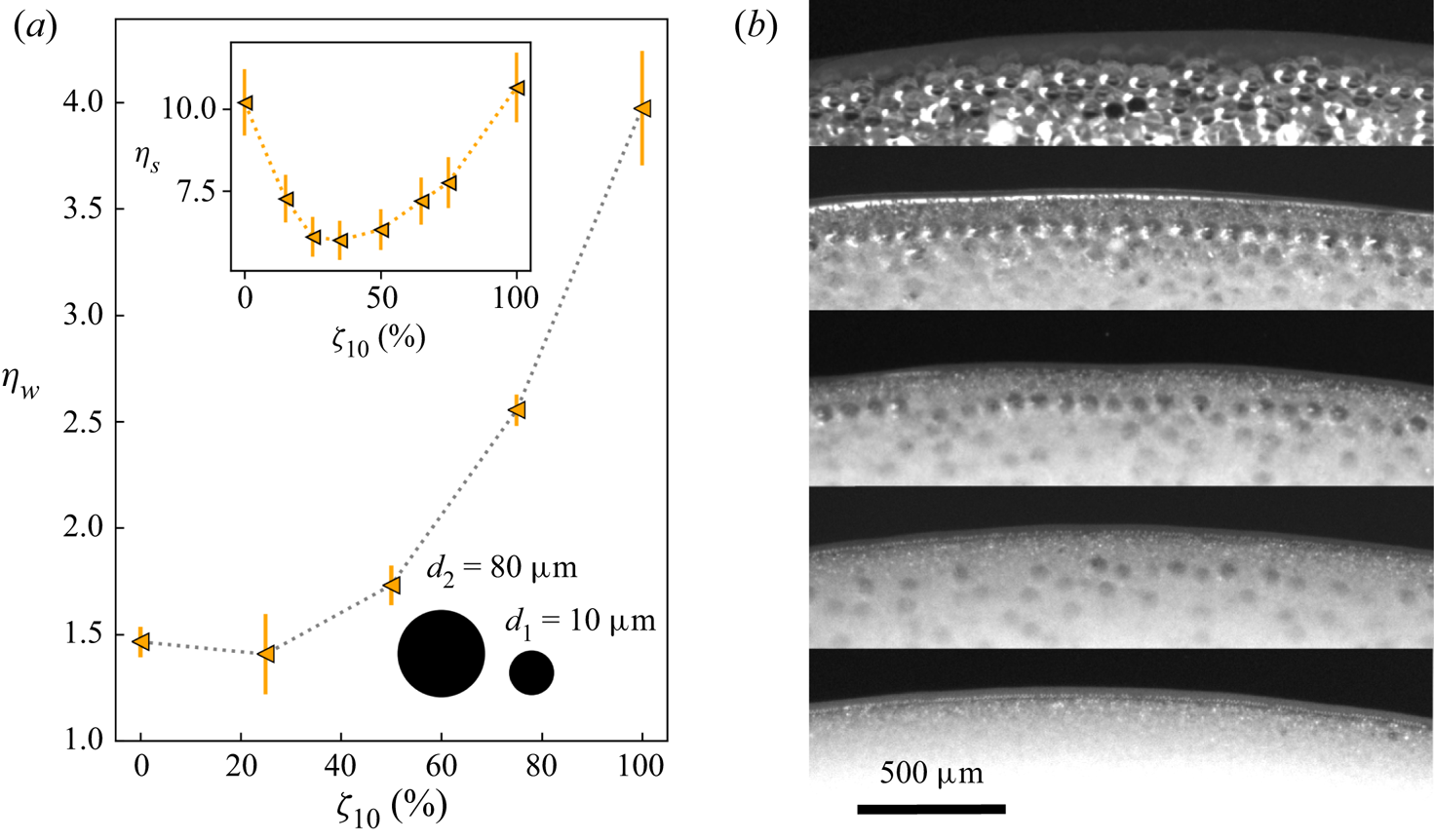
Top-view pictures of the suspension near the moving contact line provide information about the origin of the discrepancy between the apparent viscosity extracted from bulk rheology and its counterpart extracted from the dynamics of spreading; see figure 7(b). As shown previously in the monomodal case (Zhao et al. Reference Zhao, Oléron, Pelosse, Limat, Guazzelli and Roché2020), there is a pure-fluid region devoid of particles near the contact line. We observe a similar region in the monomodal and bimodal cases depicted in figure 7(b). The extent of this region is larger in the case of the 80 $\mathrm {\mu }$m particles, $\zeta _{10}=0\,\%$ (top picture), than in the 10 $\mathrm {\mu }$m case, $\zeta _{10}=100\,\%$ (bottom picture). For intermediate values of $\zeta _{10}$, the 10 $\mathrm {\mu }$m particles are able to move in between the 80 $\mathrm {\mu }$m particles. The particles closest to the contact line arrange in an orderly, crystalline structure. This ordering is particularly marked for the 80 $\mathrm {\mu }$m particles, seen in the top pictures of figure 7(b). The large 80 $\mathrm {\mu }$m particles seem to be maintained at the same distance from the contact line as small 10 $\mathrm {\mu }$m particles are added, i.e. as $\zeta _{10}$ is increased, but their linear density decreases.

The images displayed in figure 7(b) are obtained for the same dynamic contact angle $\theta _{app}=35^{\circ }$. The real capillary number of all these experiments (using the effective viscosity of the suspension, $Ca = \eta _w\,Ca_0$) is thus constant, and equal here to approximately $2\times 10^{-3}$, leading to $h^\star \sim 100\,\mathrm {\mu }$m according to (2.10) and using the prefactor inferred from figure 5(d), i.e. $h^\star \simeq 0.3 \ell _c\,Ca^{1/3}$. The discrepancy between the viscosity measured in the bulk and that estimated from spreading experiments is now clear. The 80 $\mathrm {\mu }$m particles experience strong confinement in the viscous–capillary region since $h^\star \sim d_{2}$, and only a few of them can penetrate this region. In contrast, $h^\star$ is 10 times larger than the diameter of the 10 $\mathrm {\mu }$m particles. Even if these small particles experience confinement close to the contact line, a significant part of the viscous–capillary region is filled with a dense phase of small particles akin to a suspension bulk. Thus the contribution of the 10 $\mathrm {\mu }$m particles to dissipation in the Cox–Voinov region is expected to be larger than that of the 80 $\mathrm {\mu }$m particles, as reported in experiments with monomodal suspensions. In the case of the bimodal suspensions studied in this section, increasing the small particle fraction $\zeta _{10}$ is expected to lead to a continuous increase in $\eta _w$, as observed in figure 7(a).

5.2. Varying the size of the large particles

We now turn to bimodal suspensions consisting of 10 $\mathrm {\mu }$m particles but with large particles of variable diameter (i.e. $d_2= 20, 40, 80\,\mathrm {\mu }$m) at $\zeta _{small}=25\,\%$. Bimodal suspensions formulated this way should have a bulk viscosity close to the minimum observed on the curves of figure 2(b). Figure 8(a) shows that the apparent wetting viscosity of these suspensions is maximum in the monomodal case, and decreases for bimodal suspensions as the large particle size increases, i.e. with increasing $d_2/d_1$. This result again confirms that particles with a diameter much smaller than $h^\star$ increase the dissipation in the Cox–Voinov region. This trend is similar to that of the bulk viscosity $\eta _s$, with increasing $d_2/d_1$ for $\zeta _{small}=25\,\%$; see the inset of figure 8(a). However, the magnitude of the size-ratio effect comes from two distinct physical origins. For example, the value of the apparent wetting viscosity $\eta _w$ for $d_2/d_1=8$ is close to that of the suspending fluid, whereas the value of the bulk viscosity $\eta _s$ is much larger. The decrease of the bulk viscosity comes from the size ratio affecting the maximum packing fraction $\phi _c$ (larger for large $d_2/d_1$), while the wetting viscosity reduction comes from confinement effects near the contact line as the dissipation is greater for particles that can efficiently reach the dissipation region near the contact line ($d\ll h^\star$). In the case of figure 8, the small particles are participating less in the dissipation as $\zeta _{10}$ is small and the overall dissipation is set mostly by the large particles.

Figure 8.

Experimental results for $10\,\mathrm {\mu }$m monomodal suspension ($\bullet$ symbols) and bimodal blends with ${d_1=10\,\mathrm {\mu }}$m and varying $d_2$ ($= 20$, 40, 80 $\mathrm {\mu }$m) at fixed $\zeta _{10}=25\,\%$ and $\phi =0.4$ ($\square$ symbols). (a) Relative wetting viscosity $\eta _w$ as a function of the size ratio $d_2/d_1$. The horizontal dashed line indicates the viscosity value for the monomodal suspension consisting of the sole small particles of size $10\,\mathrm {\mu }$m. Inset: bulk viscosity $\eta _s$ of the corresponding suspensions versus $d_2/d_1$. The grey dotted lines are guides for the eyes. (b) Distance of approach of the large particles for the bimodal suspensions with $d_1=10\,\mathrm {\mu }$m and $\zeta _{10}=25\,\%$ ($\square$ symbols) and the $10\,\mathrm {\mu }$m monomodal suspension ($\bullet$ symbol). The dashed line corresponds to the geometrical prediction (5.1). (c) Top-view pictures taken when $\theta _{app}=35^{\circ }$ at $h=50\,\mathrm {\mu }$m for monomodal suspension of size $10\,\mathrm {\mu }$m and bimodal suspensions with $(d_1,\zeta _{10})=(10\,\mathrm {\mu }{\rm m}, 25\,\%)$ and $d_2 = 20, 40, 80\,\mathrm {\mu }$m (from bottom to top, respectively).

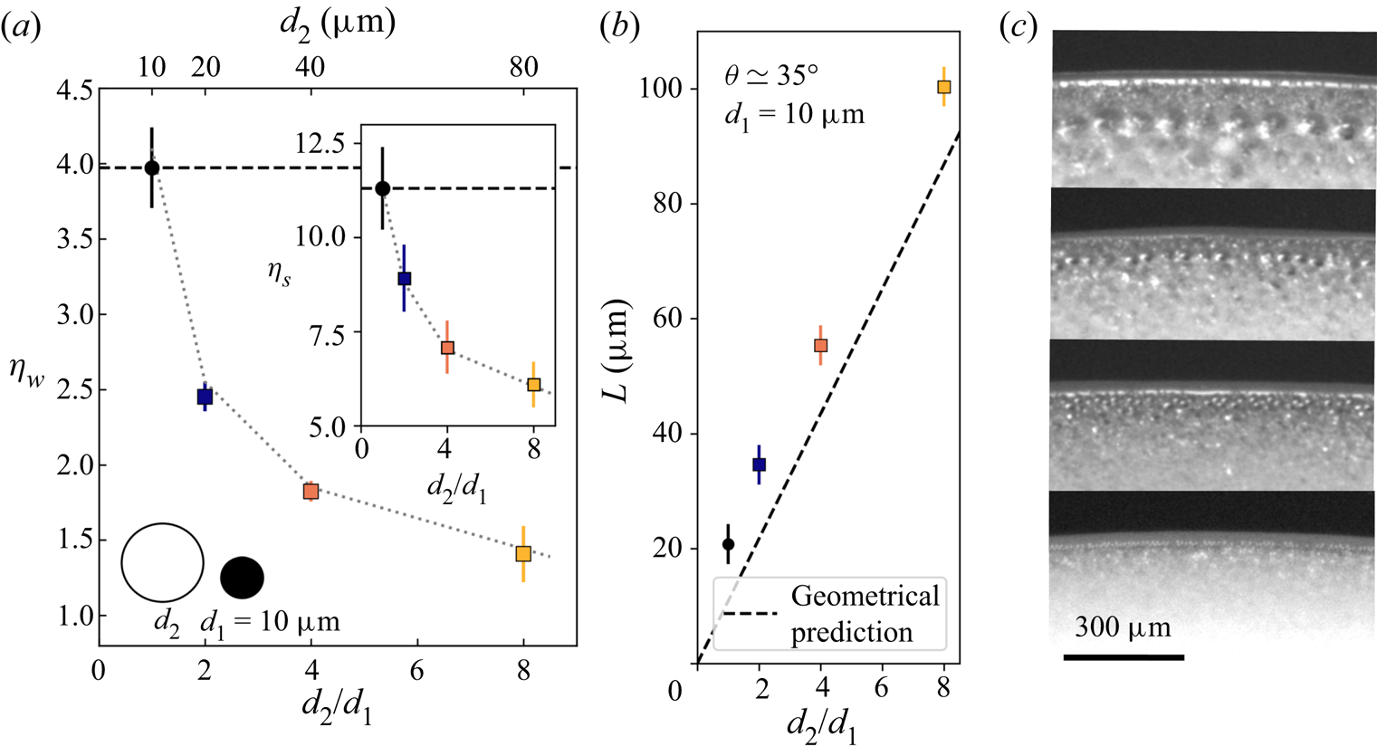
Figure 8(b) shows that the distance of approach of the large particles, $L$, increases with their diameter. This measured length follows the prediction of a geometrical model describing the minimal distance of approach of a particle in a wedge,

(5.1)\begin{equation} L=\frac{d}{2}\left[\frac{1}{\sin(\theta_{app})}+\frac{1}{\tan(\theta_{app})}-1\right], \end{equation}

where $\theta _{app}$ is the apparent contact angle near the contact line. We find that this distance is not affected sensibly by the presence of the small particles. The relation (5.1) holds for both monomodal and bimodal cases using the diameter of the corresponding particles. In the monomodal case, it determines the size of the depleted region (Zhao et al. Reference Zhao, Oléron, Pelosse, Limat, Guazzelli and Roché2020).

The top-view pictures in figure 8(c) confirm the existence of size segregation at the contact line as already mentioned in § 5.1. The large particles form ordered rows behind the small particle region as already noted in § 5.1. However, we observe that the 10 $\mathrm {\mu }$m particles do not go through the network formed by the 20 $\mathrm {\mu }$m particles; see the bottom image of figure 8(c). We move to this aspect of suspension spreading in the following subsection, with clearer visualisations with larger particles.

5.3. Varying the size of the small particles

Figure 9(a) gathers the wetting viscosity $\eta _w$ of the monomodal 80 $\mathrm {\mu }$m suspension and bimodal blends having a fixed $d_2=80\,\mathrm {\mu }$m and varying $d_1$, and $\zeta _{small}$. When the solid phase consists mainly of small particles ($\zeta _{small}=75\,\%$), $\eta _w$ decreases with increasing $d_1$, as seen in figure 9(a). This observation confirms again that the wetting viscosity is set by the possibility of particles having diameter much smaller than $h^\star$ approaching close to the contact line. However, a continuous decrease of $\eta _w$ with $d_1$ is absent when $\zeta _{small}=25\,\%$ or $\zeta _{small}=50\,\%$, i.e. when large particles constitute a significant portion of the solid blend. The relative wetting viscosity $\eta _w$ reaches a maximum around $d_1/d_2=0.25$, but it otherwise shows low values, even lower than those obtained for the monomodal suspensions of 80 $\mathrm {\mu }$m particles for $d_1/d_2 = 0.5$. In other words, for $\zeta _{small}=25\,\%\unicode{x2013}50\,\%$, the apparent wetting viscosity of the 10–80 and 40–80 $\mathrm {\mu }$m blends are particularly low compared to that of the 20–80 $\mathrm {\mu }$m and even to that of the monomodal 80 $\mathrm {\mu }$m suspension.

Figure 9.

Experimental results for suspension blends with $d_2=80\,\mathrm {\mu }$m and varying $d_1$ ($= 10, 20, 40\,\mathrm {\mu }$m) at $\zeta _{small}=25\,\%$ ($\square$ symbols), $\zeta _{small}=50\,\%$ ($\lozenge$ symbols), and $\zeta _{small}=75\,\%$ ($\triangle$ symbols). (a) Relative wetting viscosity $\eta _w$ as a function of $d_1/d_2$. The dashed line indicates the viscosity value for the monomodal suspension consisting of the sole large particles of size $80\,\mathrm {\mu }$m. Inset: bulk viscosity of the corresponding suspensions. (b,c) Top-view pictures taken when $\theta _{app}=35^{\circ }$ at $h=50\,\mathrm {\mu }$m for bimodal suspensions, with $d_2=80\,\mathrm {\mu }$m, $\zeta _{small}=25\,\%$ (b), and $\zeta _{small}=75\,\%$ (c). Small particle size is increasing from top to bottom ($d_1=10, 20, 40\,\mathrm {\mu }$m, and monomodal suspension of size $80\,\mathrm {\mu }$m).

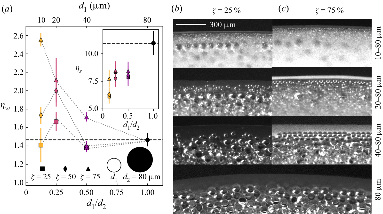
The top views shown in figure 9(b) provide some clues about the variation of the apparent wetting viscosity. At $\zeta _{small}=25\,\%$, for small values of $d_1/d_2$ (top two pictures), small particles flow through the large particle network and get close to the contact line. In contrast, for $d_1/d_2=0.5$ (third picture from the top), the presence of 40 $\mathrm {\mu }$m particles disrupts the ordering of the 80 $\mathrm {\mu }$m particles, compared to the other cases. A similar trend is observed for $\zeta _{small}=50\,\%$. In contrast, for $\zeta _{small}=75\,\%$, there is a large amount of ordered small particles near the contact line in front of the large spheres, as seen in figure 9(c).

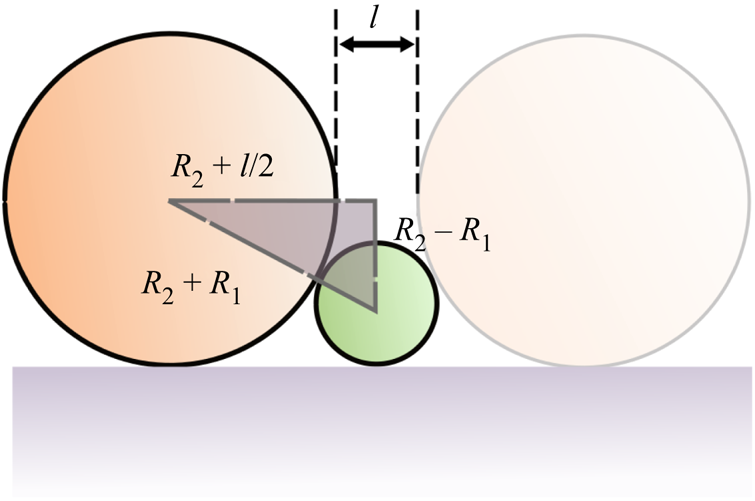
Geometrical considerations can explain the effect observed for $d_1/d_2=0.5$. Two large particles with radius $R_2=d_2/2$ sitting on the surface of a solid come to contact if the distance $l$ between them goes to zero; see figure 10. A small particle of radius $R_1$ can pass through the hole between the two particles and the solid surface if its radius is at most $R_1=R_2/4$. Consequently, while the 10 and 20 $\mathrm {\mu }$m particles can flow through the interstices created by the large 80 $\mathrm {\mu }$m particles, the 40 $\mathrm {\mu }$m particles cannot. Instead, these particles induce defects in the 80 $\mathrm {\mu }$m particle network, leading to the distortion of the large-particle matrix when the portion of small particles is not too large ($\zeta _{small} \lesssim 50\,\%$). This loss of organisation seems detrimental to the local dissipation. These geometrical considerations coupled with the wetting viscosity measurements suggest that the structure and therefore the local solid volume fraction near the contact line is a key element to explain the value of the wetting viscosity of granular suspensions.

Figure 10.

Sketch of two large particles separated by a small one on a solid plane.

However, the above geometrical arguments cannot explain the lower values of $\eta _w$ for the 10–80 $\mathrm {\mu }$m blends compared to those of the 20–80 $\mathrm {\mu }$m blends for $\zeta _{small}=25\unicode{x2013}50\,\%$ in figure 9(a). Instead, this lessening effect may be attributed to bulk effects impacting on the variation of the wetting viscosity. The inset of figure 9(a) indicates that the bulk viscosity is significantly smaller for the 10–80 $\mathrm {\mu }$m blends than for the 20–80 $\mathrm {\mu }$m blends for a given value of $\zeta _{small}$. Moreover, the bulk viscosity for $\zeta _{small}=25\unicode{x2013}50\,\%$ is lower than for $\zeta _{small}=75\,\%$ as it corresponds to the minimum bulk viscosity for bimodal blends, as seen in figure 2(b). Bulk effects are therefore evidenced in this specific example and impact the value of $\eta _w$ as they happen to overcome size effects.

It is worth noting that in the monomodal case, variation of the wetting viscosity can come only from the confinement effect near the contact line, as the bulk viscosity does not vary with particle size, as shown in figure 2(a). The case of fixed $d_2$ and increasing $d_1$ evidences two competing effects: confinement effect governing the particle ability to approach the contact line, and the variation of the bulk viscosity with $\zeta _{small}$ and $d_1/d_2$. In conclusion, for bimodal suspensions, a high wetting viscosity results from a complex compromise between a high fraction of small particles $\zeta _{small}$, a large size ratio $d_2/d_1$, and a high bulk viscosity $\eta _s$, in addition to size effects already demonstrated.