


1. Introduction
Ducted propellers utilise a stationary nozzle for increased efficiency, especially at low advance coefficients, resulting from higher rotational speeds than design. Thanks to the increasing power of supercomputers, during the last years several studies relying on high-fidelity numerical simulations were reported on conventional, non-ducted marine propellers (Balaras et al. Reference Balaras, Schroeder and Posa2015; Kumar & Mahesh Reference Kumar and Mahesh2017; Posa et al. Reference Posa, Broglia, Felli, Falchi and Balaras2019b , Reference Posa, Broglia and Balaras2022a ; Wang et al. Reference Wang, Wu, Gong and Yang2021, Reference Wang, Liu, Wang and Li2022b , Reference Wang, Liu, Guo, Li and Liao2023a ; Posa Reference Posa2022a , Reference Posa and Broglia2023a ), having the purpose of analysing their wake properties. However, the literature on ducted propellers is significantly more limited. To date, most works on the subject deal with the global performance of propulsion, with little discussion of the flow physics in their wake, whose simulation requires high-fidelity, computationally expensive methodologies and fine resolutions downstream of the propeller plane, to resolve the dynamics of the vortices they shed. In comparison with conventional propellers, the flow physics of ducted propellers is complicated by the interaction of their blades with the nozzle, giving rise to tip leakage vortices. Their dynamics is expected to differ from that of the more typical tip vortices shed by conventional propellers. This dynamics is important, affecting the signature of the propellers. The tip vortices are areas of local minima of pressure, with the potential of triggering cavitation phenomena, having detrimental effects on the structural integrity of the blades of the propeller and downstream bodies, as rudders. In addition, these phenomena substantially reinforce the acoustic signature of marine propulsion, having a negative impact on the environment and the stealth capabilities of military vessels.
The current literature on ducted propellers includes a number of works where their performance is analysed by using potential flow techniques (Baltazar & Falcão de Campos Reference Baltazar and Falcão de Campos2009; Baltazar et al. Reference Baltazar, Falcão de Campos and Bosschers2012, Reference Baltazar, Rijpkema, Falcão de Campos and Bosschers2013, Reference Baltazar, Rijpkema, Falcão de Campos and Bosschers2018; Yu et al. Reference Yu, Greve, Druckenbrod and Abdel-Maksoud2013; Kim et al. Reference Kim, Kinnas and Du2018). In other simplified approaches, relying on the axial momentum theory, actuator disk models are utilised to represent the action of the propeller blades on the flow, as in the works by Bontempo et al. (Reference Bontempo, Cardone and Manna2016) and Bontempo & Manna (Reference Bontempo and Manna2018), where the effect on performance of both decelerating and accelerating nozzles is analysed. Some other studies utilise potential methods (Bosschers et al. Reference Bosschers, Willemsen, Peddle and Rijpkema2015; Kim & Kinnas Reference Kim and Kinnas2022; Jin et al. Reference Jin, Wang, Dong, An and Xia2023) or actuator disk representations of the propeller (Gaggero et al. Reference Gaggero, Villa, Tani, Viviani and Bertetta2017; Cai et al. Reference Cai, Mao, Xu, Chai, Tian and Qiu2022), coupled with the Reynolds-averaged Navier--Stokes (RANS) technique, to capture a few more details of the flow physics. Coupled potential flow and RANS solvers were also exploited by Kinnas et al. (Reference Kinnas, Jeon, Purohit and Tian2013) to study the performance of a ducted propeller in cavitating conditions and subject to an inclined inflow. The RANS technique was utilised by Stark et al. (Reference Stark, Shi and Atlar2021), where the propeller was represented by a system of body forces during the process of optimisation of the leading edge tubercles of its nozzle. Then, fully resolved RANS was adopted for further analysis on the optimal geometry.
Fully resolved RANS was also employed in Sánchez Caja et al. (Reference Sánchez Caja, Rautaheimo and Siikonen2000), Abdel-Maksoud & Heinke (Reference Abdel-Maksoud and Heinke2002), Haimov et al. (Reference Haimov, Vicario and Del Corral2011), Bhattacharyya et al. (Reference Bhattacharyya, Neitzel, Steen, Abdel-Maksoud and Krasilnikov2015, Reference Bhattacharyya, Krasilnikov and Steen2016), Yongle et al. (Reference Yongle, Baowei and Peng2015), Motallebi-Nejad et al. (Reference Motallebi-Nejad, Bakhtiari, Ghassemi and Fadavie2017), Liu & Vanierschot (Reference Liu and Vanierschot2021). In all these studies, which focus on propeller performance, little or no information on the wake features is reported. The above numerical techniques, although well suited to handle the problem of performance prediction, are not designed to reproduce accurately the complex wake dynamics of marine propellers. In the particular case of ducted propellers, this is further complicated by the presence of the nozzle. Since in RANS-based approaches most turbulent scales are modelled, rather than resolved, this is not the best strategy for reproducing the complex unsteady dynamics that characterise the instability phenomena of the typical vortices shed by marine propellers. Better options are represented by detached eddy simulation (DES) and especially large eddy simulation (LES), where all large energy-carrying structures of the flow are explicitly resolved, while subgrid scale (SGS) modelling is limited to the only scales smaller than grid spacing. However, among the RANS studies reported on the subject of ducted propellers, Villa et al. (Reference Villa, Gaggero, Tani and Viviani2020) were able to provide some more information on the wake flow by using a computational grid consisting of 7 million finite volumes, in the framework of an adaptive mesh refinement technique, to simulate propellers with and without accelerating and decelerating nozzles. They found that both nozzles resulted in a reduced intensity of the tip vortices and the onset of additional helical structures, contributing to a more complex wake system, in comparison with the same propellers working without a duct. The interaction between the two helical vortices shed by the tip of each blade of the ducted propellers produced roll-up phenomena between them. In the wake, they approached each other and eventually merged into a single vortex.
During recent years, eddy-resolving methodologies, especially DES, were exploited to capture more accurately the dynamics of the tip vortices, their instability and to gain an improved insight on the wake physics of ducted propellers. In the work by Gong et al. (Reference Gong, Guo, Zhao, Wu and Song2018), DES was employed to compare the wake evolution of ducted and non-ducted propellers, reporting results from simulations on a computational grid consisting of 9.5 million cells. They found that the interaction of the tip vortices with the duct accelerated auto-inductance and mutual inductance phenomena, vortex pairing and in turn the instability of the wake system. The shear layer shed by the nozzle promoted the onset of additional secondary vortices, creating a bridge between tip vortices. In addition, wake contraction was reduced, as demonstrated by the larger distance of the core of the tip vortices from the wake axis, in comparison with the case of the same propeller working without a nozzle. The same approach was utilised by Gong et al. (2021) to study the influence of the number of blades on the wake features, by considering ducted propellers consisting of one, two and four blades, respectively. They verified faster grouping phenomena of the tip vortices for increasing blades numbers, as a result of their decreasing inter-spiral distance. In this study, the comparison with the cases of non-ducted propellers confirmed the role of the nozzle in accelerating the instability of the tip vortices.
Delayed DES was adopted by both Zhang & Jaiman (Reference Zhang and Jaiman2019) and Shi et al. (Reference Shi, Wang, Zhao and Zhang2022) to investigate the wake dynamics on computational grids consisting of 33 million cells. The instability of the wake system was studied by Zhang & Jaiman (Reference Zhang and Jaiman2019) across a range of values of advance coefficient, finding that it is accelerated for decreasing values, as expected from the behaviour also observed in earlier studies on conventional, non-ducted propellers. Shi et al. (Reference Shi, Wang, Zhao and Zhang2022) highlight that the shear with the nozzle reduces the intensity of the tip vortices. However, in contrast with earlier studies, they found an increased inter-spiral distance, which has the affect of delaying the onset of instability phenomena. In a later study relying on the same numerical approach (delayed DES), computational grids of up to approximately 40 million cells were adopted by Wang et al. (Reference Wang, Shi, Zhao and Zhang2023b
) to study the same ducted propeller working within inflows at angles ranging from $0^\circ$
to
$0^\circ$
to $60^\circ$
, including again comparisons between the cases of propellers with and without a nozzle. They reported that the nozzle has the effect of reducing the wake deflection and mitigating the asymmetry between the leeward and windward sides of the wake. In addition, the nozzle results in a reduced frequency of wake meandering. Chen et al. (Reference Chen, Liu, Si, Liang, Jin and Yuan2022) utilised DES and the Ffowcs Williams--Hawkings acoustic analogy (Ffowcs Williams & Hawkings Reference Ffowcs Williams and Hawkings1969) to reconstruct the acoustic signature of a ducted propeller, exploiting results of simulations on a grid consisting of 10 million elements. They found that the efficiency of propulsion was initially increased and then reduced for increasing values of the advance coefficient. A similar trend was verified for the sound pressure levels, which were the smallest at the condition of best efficiency and the largest in the bollard pull condition, with the propeller operating at zero advance velocity.
$60^\circ$
, including again comparisons between the cases of propellers with and without a nozzle. They reported that the nozzle has the effect of reducing the wake deflection and mitigating the asymmetry between the leeward and windward sides of the wake. In addition, the nozzle results in a reduced frequency of wake meandering. Chen et al. (Reference Chen, Liu, Si, Liang, Jin and Yuan2022) utilised DES and the Ffowcs Williams--Hawkings acoustic analogy (Ffowcs Williams & Hawkings Reference Ffowcs Williams and Hawkings1969) to reconstruct the acoustic signature of a ducted propeller, exploiting results of simulations on a grid consisting of 10 million elements. They found that the efficiency of propulsion was initially increased and then reduced for increasing values of the advance coefficient. A similar trend was verified for the sound pressure levels, which were the smallest at the condition of best efficiency and the largest in the bollard pull condition, with the propeller operating at zero advance velocity.
As discussed above, a few eddy-resolving DES studies on ducted propellers are currently available in the literature. In this work, to the authors’ knowledge, we report results of the first LES computations on the subject. We rely on far more extensive computational grids than in the earlier studies, using a cylindrical grid consisting of 3.5 billion points in the framework of an immersed boundary (IB) technique. As demonstrated in the following discussion, this strategy allowed us to resolve explicitly most turbulence, limiting the modelling assumptions to only the smallest, dissipative scales of the flow. This is especially important in the present case, where high levels of anisotropy of turbulence are expected, in particular in the region of shear between the tip leakage vortices and the inner surface of the nozzle. These flow conditions are well known to be a challenge for more conventional modelling strategies, as those adopted in RANS approaches. Meanwhile, performing physical measurements within the region of the gap between the blades tip and the surface of the nozzle is very problematic, as demonstrated by the few experimental studies currently available in the literature on ducted marine propellers, where they are usually limited to the analysis of global performance (Bhattacharyya & Steen Reference Bhattacharyya and Steen2014a , Reference Bhattacharyya and Steenb ; Chen et al. Reference Chen, Liu, Si, Liang, Jin and Yuan2022) and visualisations of cavitation phenomena in the region of the tip gap (Gaggero et al. Reference Gaggero, Rizzo, Tani and Viviani2013). For instance, Villa et al. (Reference Villa, Gaggero, Tani and Viviani2020), which is the most detailed work in the field, reports experimental data, but only for the first-order statistics of the wake flow, downstream of the nozzle.
In the present study, the wealth of details on the wake flow is exploited to compare the wake dynamics of ducted and non-ducted propellers. A detailed vortex core analysis is conducted, missing in the above literature on ducted marine propellers. We show that the evolution of the tip leakage vortices shed by the ducted propeller is substantially influenced by their shear with the boundary layer on the inner surface of the duct. This has important consequences on their trajectory, turbulent stresses and instability, if compared with the tip vortices shed by conventional propellers. The correlation between the turbulent statistics at the core of the tip leakage vortices and their interaction with the boundary layer on the duct are not discussed in the earlier literature, due to limitations affecting both the numerical technique and the resolution of the computational grid. This is the case even when more accurate DES methodologies are adopted. About this point, it should be acknowledged that Gong et al. (Reference Gong, Guo, Zhao, Wu and Song2018) and Shi et al. (Reference Shi, Wang, Zhao and Zhang2022) indeed reported upon an in-depth analysis at probes placed on the trajectory of the tip leakage vortices, based on data from DES computations. Unfortunately, in these studies only locations downstream of the nozzle were considered, excluding the important region of shear with its boundary layer, and data were limited to the kinetic energy within the tip leakage vortices and its spectra in time. In contrast, the results of the present study demonstrate that the early stages of development of the tip leakage vortices within the nozzle of ducted propellers are critical in affecting their faster instability and diffusion, in comparison with the more typical tip vortices shed by conventional propellers. Tip and tip leakage vortices play a critical role in the overall performance of propellers and rotating machinery devices in general. They are locations of pressure minima and large turbulent stresses, affecting cavitation phenomena as well as their instability and, in turn, the acoustic signature of the system. The tip leakage vortices shed by ducted propellers are expected to be less intense than the tip vortices shed by conventional propellers producing the same thrust, since part of the load is transferred from the rotor to the nozzle. Meanwhile, the acceleration of the flow within the small gap between the blades tip and nozzle as well as the shear of the tip leakage vortices with the surface of the nozzle have the potential to reinforce pressure minima, turbulence and instability. The outcome of the balance between these opposite effects is not well known and is discussed in depth in the present study, distinguishing between the phenomena occurring within the nozzle, where the interaction between its inner surface and the tip leakage vortices occurs, and the locations further downstream, where the instability and diffusion of the tip leakage vortices is accelerated, in comparison with that of the tip vortices shed by conventional propellers. In addition, details dealing with the flow conditions produced on the surface of the propeller blades, as a result of the acceleration of the flow promoted by the nozzle, are discussed. These phenomena have a substantial impact on the wake dynamics, since they lead to the onset of weaker tip leakage vortices. Nonetheless, a detailed analysis of the flow over the blades of ducted propellers is also missing in the earlier studies on the subject, which are more focused on their wake features. These changes affecting the flow through ducted propellers, analysed in the present study, are the sources of the substantial deviations between the wake developments of propellers operating with and without a nozzle.
In the following sections we discuss the methodology (§ 2), the flow problem (§ 3), the computational set-up (§ 4), the results of the simulations (§ 5) and the conclusions from the present study (§ 6).
2. Methodology
The filtered Navier--Stokes equations (NSEs) for incompressible flows were resolved in non-dimensional form:
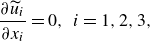 \begin{align} {\partial \widetilde {u}_i \over \partial x_i} = 0, \;\;\; &i=1,2,3, \end{align}
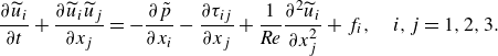 \begin{align} {\partial \widetilde {u}_i \over \partial t} + {\partial \widetilde {u}_i \widetilde {u}_j \over \partial x_j } = - {\partial \tilde {p} \over \partial x_i} - {\partial \tau _{ij} \over \partial x_j} &+ {1 \over \textit {Re}} {\partial ^2 \widetilde {u}_i \over \partial x_j^2} + f_i, \quad i,j=1,2,3. \end{align}
Here (2.1) and (2.2) represent the conservation of mass and momentum, respectively, and the indexes $i$
and
$i$
and $j$
refer to the three directions in space. In (2.1) and (2.2),
$j$
refer to the three directions in space. In (2.1) and (2.2), $x_i$
and
$x_i$
and $x_j$
are the coordinates in space along the directions
$x_j$
are the coordinates in space along the directions $i$
and
$i$
and $j$
,
$j$
, $t$
is time,
$t$
is time, $\widetilde {u}_i$
and
$\widetilde {u}_i$
and $\widetilde {u}_j$
are the filtered velocity components in the directions
$\widetilde {u}_j$
are the filtered velocity components in the directions $i$
and
$i$
and $j$
,
$j$
, $ \tilde {p}$
is the filtered pressure,
$ \tilde {p}$
is the filtered pressure, $\tau _{ij}$
is the
$\tau _{ij}$
is the $ij$
element of the SGS stress tensor,
$ij$
element of the SGS stress tensor, $\textit {Re}$
is the Reynolds number and
$\textit {Re}$
is the Reynolds number and $f_i$
is the component in the direction
$f_i$
is the component in the direction $i$
of a forcing term. The Reynolds number comes from scaling the dimensional NSEs by using the density of the fluid,
$i$
of a forcing term. The Reynolds number comes from scaling the dimensional NSEs by using the density of the fluid, $\rho$
, a reference length scale,
$\rho$
, a reference length scale, $L$
, and a reference velocity scale,
$L$
, and a reference velocity scale, $U$
. It is defined as
$U$
. It is defined as $Re=UL/\nu$
, where
$Re=UL/\nu$
, where $\nu$
is the kinematic viscosity of the fluid.
$\nu$
is the kinematic viscosity of the fluid.
The SGS stress tensor, $\tau _{ij}=\widetilde {\,u_iu_j\,}\!-\widetilde {u}_i\widetilde {u}_j$
, comes from filtering the NSEs, that is from resolving them on a computational grid that is coarser than the Kolmogorov scale, which is the smallest scale of the flow. This is almost always the case in problems of interest in engineering. Therefore, the SGS tensor represents the action of the smallest, unresolved scales of the flow on the largest ones that the computational grid is able to resolve. This tensor needs to be modelled. In this study, this is achieved by considering an eddy-viscosity assumption. The deviatoric part of the SGS tensor is assumed to be proportional to the deformation tensor of the resolved velocity field
$\tau _{ij}=\widetilde {\,u_iu_j\,}\!-\widetilde {u}_i\widetilde {u}_j$
, comes from filtering the NSEs, that is from resolving them on a computational grid that is coarser than the Kolmogorov scale, which is the smallest scale of the flow. This is almost always the case in problems of interest in engineering. Therefore, the SGS tensor represents the action of the smallest, unresolved scales of the flow on the largest ones that the computational grid is able to resolve. This tensor needs to be modelled. In this study, this is achieved by considering an eddy-viscosity assumption. The deviatoric part of the SGS tensor is assumed to be proportional to the deformation tensor of the resolved velocity field
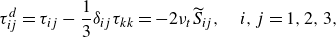 \begin{equation} \tau _{ij}^d = \tau _{ij} - {1 \over 3} \delta _{ij} \tau _{kk} = -2 \nu _t \widetilde {S}_{ij}, \quad i,j=1,2,3, \end{equation}
where $\delta _{ij}$
is the Kronecker delta,
$\delta _{ij}$
is the Kronecker delta, $\tau _{kk}$
is the trace of the SGS tensor,
$\tau _{kk}$
is the trace of the SGS tensor, $\nu _t$
is the eddy viscosity and
$\nu _t$
is the eddy viscosity and $\widetilde {S}_{ij}$
is the deformation tensor of the resolved velocity field
$\widetilde {S}_{ij}$
is the deformation tensor of the resolved velocity field
 \begin{equation} \widetilde {S}_{ij} = {1 \over 2} \left ( {\partial \widetilde {u}_i \over \partial x_j} + {\partial \widetilde {u}_j \over \partial x_i} \right ), \;\;\;i,j=1,2,3. \end{equation}
The assumption in (2.3) enables us to reduce the number of unknowns of the problem of turbulence closure from six ( $\tau _{ij}$
is symmetric) to the only eddy viscosity. This is modelled in this study by means of the wall-adaptive local eddy-viscosity (WALE) model by Nicoud & Ducros (Reference Nicoud and Ducros1999), where
$\tau _{ij}$
is symmetric) to the only eddy viscosity. This is modelled in this study by means of the wall-adaptive local eddy-viscosity (WALE) model by Nicoud & Ducros (Reference Nicoud and Ducros1999), where $\nu _t$
is computed by using the deviatoric part of the square of the gradient tensor of the resolved velocity field,
$\nu _t$
is computed by using the deviatoric part of the square of the gradient tensor of the resolved velocity field, $\widetilde {\mathcal {S}}_{ij}^d$
:
$\widetilde {\mathcal {S}}_{ij}^d$
:
 \begin{equation} \nu _t= (C_w \varDelta )^2 { ( \widetilde {\mathcal {S}}_{ij}^d \widetilde {\mathcal {S}}_{ij}^d )^{3/2} \over ( \widetilde {S}_{ij} \widetilde {S}_{ij} )^{5/2} + { ( \widetilde {\mathcal {S}}_{ij}^d \widetilde {\mathcal {S}}_{ij}^d )^{5/4}}}, \quad i,j=1,2,3. \end{equation}
Here $C_w=0.5$
is a constant, while
$C_w=0.5$
is a constant, while $\varDelta$
is the local grid spacing, computed as the cubic root of each cell of the adopted computational grid. The quantity
$\varDelta$
is the local grid spacing, computed as the cubic root of each cell of the adopted computational grid. The quantity $\widetilde {\mathcal {S}}_{ij}^d$
in (2.5) includes both contributions of strain and rotation of the resolved velocity field. This makes the WALE model able to switch off in regions of laminar gradients with no turbulence. In addition, the expression for
$\widetilde {\mathcal {S}}_{ij}^d$
in (2.5) includes both contributions of strain and rotation of the resolved velocity field. This makes the WALE model able to switch off in regions of laminar gradients with no turbulence. In addition, the expression for $\nu _t$
in (2.5) was designed to reproduce the proper limiting behaviour of
$\nu _t$
in (2.5) was designed to reproduce the proper limiting behaviour of $\nu _t$
in the vicinity of solid walls, scaling as the cubic power of the distance from the wall. This feature of the WALE model was verified in the framework of the present solver in our earlier studies (Posa & Balaras Reference Posa and Balaras2018) and is especially convenient, since it avoids the implementation of damping functions in the vicinity of solid boundaries, which may be tricky in case of complex geometries. Furthermore, this model requires only local information on the flow, which is useful to limit its computational cost. The WALE model was successfully utilised in the framework of our earlier studies on marine propellers, including also comparisons with experiments dealing with the wake flow (Posa et al. Reference Posa, Broglia, Felli, Falchi and Balaras2019b
, Reference Posa, Broglia and Balaras2022a
, Reference Posa, Capone, Alves Pereira, Di Felice and Broglia2024).
$\nu _t$
in the vicinity of solid walls, scaling as the cubic power of the distance from the wall. This feature of the WALE model was verified in the framework of the present solver in our earlier studies (Posa & Balaras Reference Posa and Balaras2018) and is especially convenient, since it avoids the implementation of damping functions in the vicinity of solid boundaries, which may be tricky in case of complex geometries. Furthermore, this model requires only local information on the flow, which is useful to limit its computational cost. The WALE model was successfully utilised in the framework of our earlier studies on marine propellers, including also comparisons with experiments dealing with the wake flow (Posa et al. Reference Posa, Broglia, Felli, Falchi and Balaras2019b
, Reference Posa, Broglia and Balaras2022a
, Reference Posa, Capone, Alves Pereira, Di Felice and Broglia2024).
The forcing term, $f_i$
, in (2.2) was utilised in the present computations to enforce the no-slip boundary condition on the surface of solid bodies, relying on an IB technique. Thanks to this approach, the Eulerian grid, discretizing the computational domain and where the NSEs are resolved, is not required to conform the geometries of the bodies immersed within the flow. They are represented by Lagrangian grids, discretizing their surface. They are ‘immersed’ and free to move within a regular Eulerian grid. Based on the position of the points of the Eulerian grid, relative to the Lagrangian grids of the bodies, the former are separated in solid, fluid and interface points. The solid points are the Eulerian points placed inside the immersed boundaries. The fluid points are the Eulerian points outside the immersed boundaries and having no neighbouring solid points. The remaining points, outside the immersed boundaries, but having neighbouring solid points, are tagged as interface points. Velocity conditions need to be enforced at the solid and interface points, while at the fluid points
$f_i$
, in (2.2) was utilised in the present computations to enforce the no-slip boundary condition on the surface of solid bodies, relying on an IB technique. Thanks to this approach, the Eulerian grid, discretizing the computational domain and where the NSEs are resolved, is not required to conform the geometries of the bodies immersed within the flow. They are represented by Lagrangian grids, discretizing their surface. They are ‘immersed’ and free to move within a regular Eulerian grid. Based on the position of the points of the Eulerian grid, relative to the Lagrangian grids of the bodies, the former are separated in solid, fluid and interface points. The solid points are the Eulerian points placed inside the immersed boundaries. The fluid points are the Eulerian points outside the immersed boundaries and having no neighbouring solid points. The remaining points, outside the immersed boundaries, but having neighbouring solid points, are tagged as interface points. Velocity conditions need to be enforced at the solid and interface points, while at the fluid points $f_i=0$
. For the solid points, this condition is the velocity of the body where those points are placed. For the interface points, it comes from a local, linear reconstruction of the velocity field along the direction normal to the body. This reconstruction utilises the no-slip requirement on the surface of the immersed boundary and the solution of the flow at the fluid points of the Eulerian grid in the vicinity of the particular interface point. Therefore, the forcing term at the solid and interface points in the momentum equation is given by
$f_i=0$
. For the solid points, this condition is the velocity of the body where those points are placed. For the interface points, it comes from a local, linear reconstruction of the velocity field along the direction normal to the body. This reconstruction utilises the no-slip requirement on the surface of the immersed boundary and the solution of the flow at the fluid points of the Eulerian grid in the vicinity of the particular interface point. Therefore, the forcing term at the solid and interface points in the momentum equation is given by
 \begin{equation} f_i = {\mathcal {V}_i - \widetilde {u}_i \over \Delta t} - \mathcal {R}_i, \;\;\; i=1,2,3, \end{equation}
where $\mathcal {V}_i$
is the velocity boundary condition to be enforced, defined as discussed above,
$\mathcal {V}_i$
is the velocity boundary condition to be enforced, defined as discussed above, $\widetilde {u}_i$
is the velocity at the particular point,
$\widetilde {u}_i$
is the velocity at the particular point, $\Delta t$
is the step of the advancement in time of the numerical solution, while
$\Delta t$
is the step of the advancement in time of the numerical solution, while $\mathcal {R}_i$
is the sum of the pressure gradient, convective, viscous and SGS terms of the momentum equation, all computed explicitly.
$\mathcal {R}_i$
is the sum of the pressure gradient, convective, viscous and SGS terms of the momentum equation, all computed explicitly.
The NSEs were discretised in space on a staggered cylindrical grid, by using second-order central finite differences. As demonstrated by Fukagata & Kasagi (Reference Fukagata and Kasagi2002), this approach is able to achieve the exact conservation of mass, momentum and energy by the discretised version of the flow problem, which is a critical requirement for the accuracy of eddy-resolving simulations. The advancement in time of the solution adopted a fractional-step technique (Van Kan Reference Van Kan1986). The discretization in time of all viscous, convective and SGS terms adopted the explicit, three-step Runge–Kutta scheme. However, to relax the otherwise prohibitive stability restrictions on the size of the time step, the terms of azimuthal derivatives in the vicinity of the wake axis, where the linear azimuthal spacing of the cylindrical grid becomes very small, were discretised by using the second-order, implicit Crank–Nicolson scheme. This was also the case for the terms of radial derivatives at the radial coordinates of the gap between the tip of the propeller blades and the duct. There, the radial grid is especially fine to resolve this small region with large gradients of the solution. More details on the grid properties will be provided later in § 4. The hepta-diagonal Poisson problem arising from the enforcement of the continuity condition was reduced to a series of penta-diagonal Poisson problems by using trigonometric transformations along the periodic azimuthal direction. Each of them was inverted by means of a direct solver, developed by Rossi & Toivanen (Reference Rossi and Toivanen1999). The overall NSEs solver was demonstrated second-order accurate in both space and time on canonical problems by Balaras (Reference Balaras2004) and Yang & Balaras (Reference Yang and Balaras2006). It was successfully utilised in a variety of cases involving marine propellers, including also validations against experiments on both performance and wake physics (Posa Reference Posa, Broglia, Felli, Cianferra and Armenio2022b , Reference Posa2023b ; Posa & Broglia Reference Posa and Broglia2022; Posa et al. Reference Posa, Broglia, Felli, Cianferra and Armenio2022b , Reference Posa, Capone, Alves Pereira, Di Felice and Broglia2024).
In this section all filtered quantities were denoted as $\tilde {\cdot }$
. Since only resolved quantities will be considered below, for convenience, this notation will be omitted hereafter.
$\tilde {\cdot }$
. Since only resolved quantities will be considered below, for convenience, this notation will be omitted hereafter.
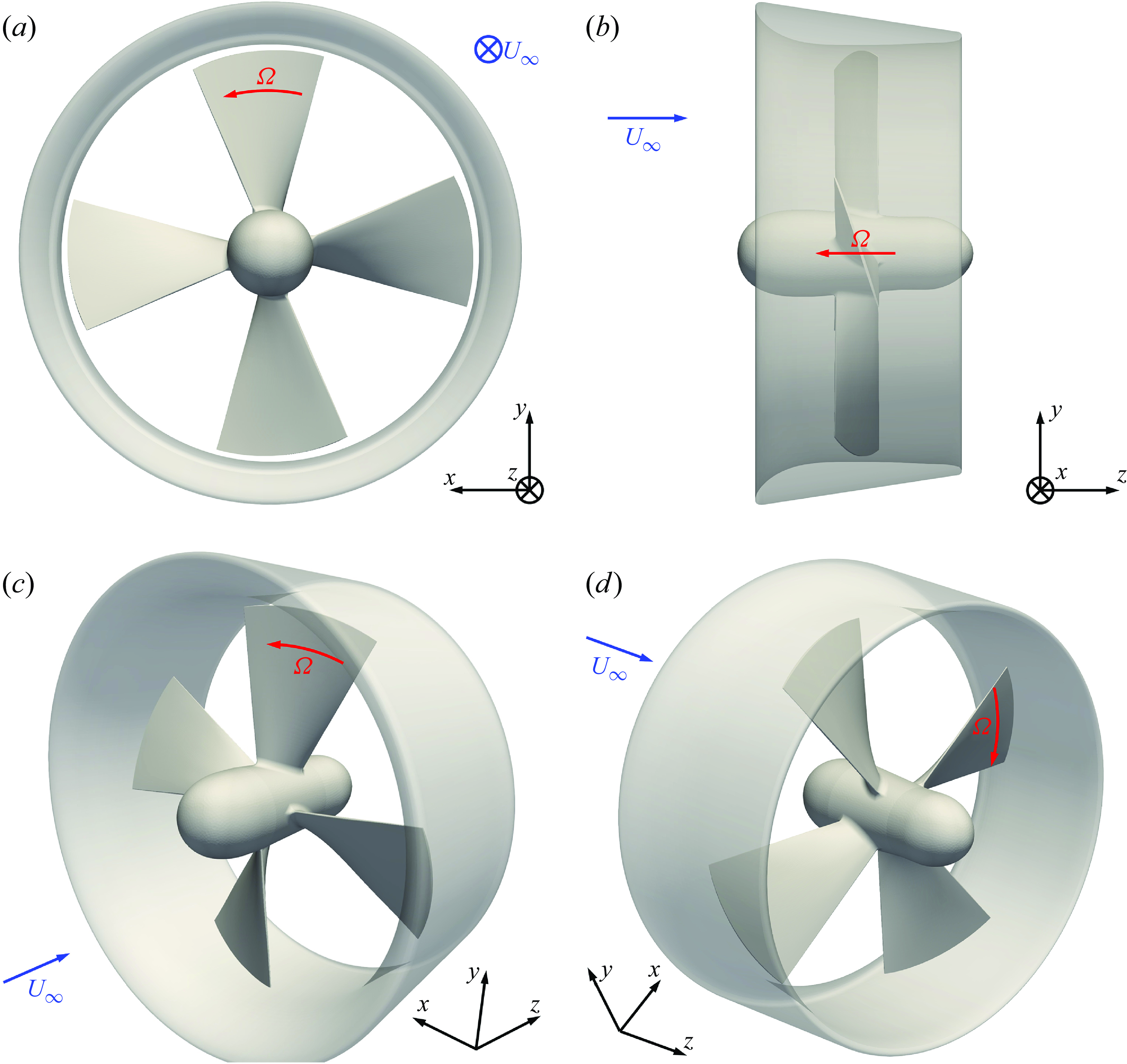
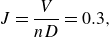
Geometry of the ducted propeller: (a) frontal view, (b) lateral view, (c) isometric view from upstream, (d) isometric view from downstream.
3. Flow problem
The geometry of the propeller considered in this study is illustrated in figure 1, where $U_\infty$
represents the free-stream velocity and
$U_\infty$
represents the free-stream velocity and $\Omega$
the angular speed of the rotor, consisting of the blades and hub of the propeller. This is a constant-pitch, four-bladed propeller (KA4 series). Its duct is the Wageningen 19A. The gap between the tip of the propeller blades and the inner surface of the duct is equivalent to
$\Omega$
the angular speed of the rotor, consisting of the blades and hub of the propeller. This is a constant-pitch, four-bladed propeller (KA4 series). Its duct is the Wageningen 19A. The gap between the tip of the propeller blades and the inner surface of the duct is equivalent to $0.0182D$
. Note that the conventional propeller is the same geometry without the duct. The working conditions of marine propellers are typically characterised through the advance coefficient,
$0.0182D$
. Note that the conventional propeller is the same geometry without the duct. The working conditions of marine propellers are typically characterised through the advance coefficient, $J$
, and the Reynolds number,
$J$
, and the Reynolds number, $Re_{70\,\%R}$
, referred to
$Re_{70\,\%R}$
, referred to $70\,\%$
of their radial extent,
$70\,\%$
of their radial extent, $R$
. They are defined as
$R$
. They are defined as
 \begin{align} &\qquad\qquad J = {V \over nD} = 0.3, \end{align}
 \begin{align} Re_p = &{c_{70\,\%R}\sqrt {(2 \pi n \; 0.7R)^2+V^2} \over \nu } \approx 360\,000, \end{align}
where $V$
is the advance velocity, in this case equal to
$V$
is the advance velocity, in this case equal to $U_\infty$
,
$U_\infty$
, $n=\Omega /2\pi$
the rotational frequency,
$n=\Omega /2\pi$
the rotational frequency, $D$
the diameter of the propeller,
$D$
the diameter of the propeller, $c_{70\,\%R}$
the chord of the propeller blades at
$c_{70\,\%R}$
the chord of the propeller blades at $70\,\%$
of its radial extent and
$70\,\%$
of its radial extent and $\nu$
the kinematic viscosity of water. It is worth noting that the definition of the Reynolds number considers as reference velocity the relative velocity of the flow at
$\nu$
the kinematic viscosity of water. It is worth noting that the definition of the Reynolds number considers as reference velocity the relative velocity of the flow at $70\,\%$
R. Both propellers were simulated in open-water conditions, which means that they ingest a uniform flow. Note also that the design working condition of the conventional propeller is
$70\,\%$
R. Both propellers were simulated in open-water conditions, which means that they ingest a uniform flow. Note also that the design working condition of the conventional propeller is $J=0.5$
. Therefore, the working condition analysed in the present study is a highly loaded condition, equivalent to a higher rotational speed than design.
$J=0.5$
. Therefore, the working condition analysed in the present study is a highly loaded condition, equivalent to a higher rotational speed than design.
(a,c) Radial and (b,d) axial resolutions of the computational grid across (a,b) the whole domain and (c,d) details in the vicinity of the propeller.

Near-wall resolution of the Eulerian grid in wall units on the (a,b) suction and (c,d) pressure sides of the (a,c) ducted and (b,d) conventional propellers.
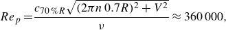
Lagrangian grids: (a) isometric view, (b) detail of the propeller blade, (c) detail of the blade tip, (d) detail of the blade root.
4. Computational set-up
Large eddy simulation computations were conducted within a cylindrical domain, having a radial extent equivalent to $5.0D$
and ranging from
$5.0D$
and ranging from $2.5D$
upstream of the propeller plane up to
$2.5D$
upstream of the propeller plane up to $5.0D$
downstream. A uniform streamwise velocity condition was enforced at the inlet section, while convective conditions were utilised at the outflow boundary of the domain, using the free-stream velocity as convective velocity. Homogeneous Neumann conditions with impermeability were imposed at the cylindrical boundary (
$5.0D$
downstream. A uniform streamwise velocity condition was enforced at the inlet section, while convective conditions were utilised at the outflow boundary of the domain, using the free-stream velocity as convective velocity. Homogeneous Neumann conditions with impermeability were imposed at the cylindrical boundary ( $u = 0$
,
$u = 0$
, $\partial v / \partial r = 0$
,
$\partial v / \partial r = 0$
, $\partial w / \partial r = 0$
, where
$\partial w / \partial r = 0$
, where $u$
,
$u$
, $v$
and
$v$
and $w$
are the radial, azimuthal and axial velocity components, respectively, while
$w$
are the radial, azimuthal and axial velocity components, respectively, while $r$
is the radial coordinate) to mimic a free stream. Homogeneous Neumann conditions were utilised at all boundaries of the domain for both pressure and eddy viscosity. Periodic conditions were enforced at the azimuthal boundaries for all flow variables.
$r$
is the radial coordinate) to mimic a free stream. Homogeneous Neumann conditions were utilised at all boundaries of the domain for both pressure and eddy viscosity. Periodic conditions were enforced at the azimuthal boundaries for all flow variables.
The domain was discretised by a cylindrical grid, consisting of $840 \times 2050 \times 2050$
(3.5 billion) points across the radial, azimuthal and axial directions, respectively. The radial and axial grids were non-uniform, to cluster points in the vicinity of the propeller and its wake. The distributions of the radial and axial grid spacings are reported in figure 2. The radial grid was uniform across the span of the propeller blades in the region
$840 \times 2050 \times 2050$
(3.5 billion) points across the radial, azimuthal and axial directions, respectively. The radial and axial grids were non-uniform, to cluster points in the vicinity of the propeller and its wake. The distributions of the radial and axial grid spacings are reported in figure 2. The radial grid was uniform across the span of the propeller blades in the region $0.00 \lt r/D \lt 0.45$
, with a resolution
$0.00 \lt r/D \lt 0.45$
, with a resolution $\Delta r/D = 1 \times 10^{-3}$
. It was refined in the vicinity of the tip of the blades, in order to achieve in the gap between them and the inner surface of the duct a resolution equivalent to
$\Delta r/D = 1 \times 10^{-3}$
. It was refined in the vicinity of the tip of the blades, in order to achieve in the gap between them and the inner surface of the duct a resolution equivalent to $\Delta r/D = 2.5 \times 10^{-4}$
, corresponding to a number of 73 Eulerian points within the gap. The region encompassing the duct was resolved by using a radial spacing
$\Delta r/D = 2.5 \times 10^{-4}$
, corresponding to a number of 73 Eulerian points within the gap. The region encompassing the duct was resolved by using a radial spacing $\Delta r/D = 1 \times 10^{-3}$
. At outer radial coordinates the grid was stretched up to the lateral boundary of the computational domain, in order to save grid points in the areas of low gradients of the solution. The axial grid was designed to achieve a resolution
$\Delta r/D = 1 \times 10^{-3}$
. At outer radial coordinates the grid was stretched up to the lateral boundary of the computational domain, in order to save grid points in the areas of low gradients of the solution. The axial grid was designed to achieve a resolution $\Delta z/D = 5 \times 10^{-4}$
in the region of the propeller blades and was slowly stretched downstream, with the purpose of resolving the flow in the near wake, up to
$\Delta z/D = 5 \times 10^{-4}$
in the region of the propeller blades and was slowly stretched downstream, with the purpose of resolving the flow in the near wake, up to $z/D=3.5$
, where
$z/D=3.5$
, where $z$
is the streamwise coordinate, whose origin was placed on the propeller plane. The angular azimuthal spacing of the grid was uniform. This is convenient, resulting in a decreasing linear spacing towards inner radii, where more resolution is required. For instance, at
$z$
is the streamwise coordinate, whose origin was placed on the propeller plane. The angular azimuthal spacing of the grid was uniform. This is convenient, resulting in a decreasing linear spacing towards inner radii, where more resolution is required. For instance, at $70\,\%$
of the radial extent of the propeller the linear azimuthal spacing of the cylindrical grid was
$70\,\%$
of the radial extent of the propeller the linear azimuthal spacing of the cylindrical grid was $0.7R\Delta \vartheta /D = 1 \times 10^{-3}$
. We verified that the average resolution of the grid was equivalent to about 4 wall units on the surface of the propeller blades and 2 wall units on the surface of the duct. Contours of near-wall resolution in inner coordinates from the simulations on the ducted and conventional propellers are shown in the left and right panels of figure 3, respectively. This level of resolution was considered adequate enough for the linear reconstruction of the velocity field at the interface points of the Eulerian grid, adopted to enforce the no slip condition on the surface of the Lagrangian grids according to the IB approach discussed earlier in § 2. Meanwhile, due to the inherent features of the IB methodology, further increasing the resolution of the Eulerian grid was not affordable, based on the available computational resources.
$0.7R\Delta \vartheta /D = 1 \times 10^{-3}$
. We verified that the average resolution of the grid was equivalent to about 4 wall units on the surface of the propeller blades and 2 wall units on the surface of the duct. Contours of near-wall resolution in inner coordinates from the simulations on the ducted and conventional propellers are shown in the left and right panels of figure 3, respectively. This level of resolution was considered adequate enough for the linear reconstruction of the velocity field at the interface points of the Eulerian grid, adopted to enforce the no slip condition on the surface of the Lagrangian grids according to the IB approach discussed earlier in § 2. Meanwhile, due to the inherent features of the IB methodology, further increasing the resolution of the Eulerian grid was not affordable, based on the available computational resources.
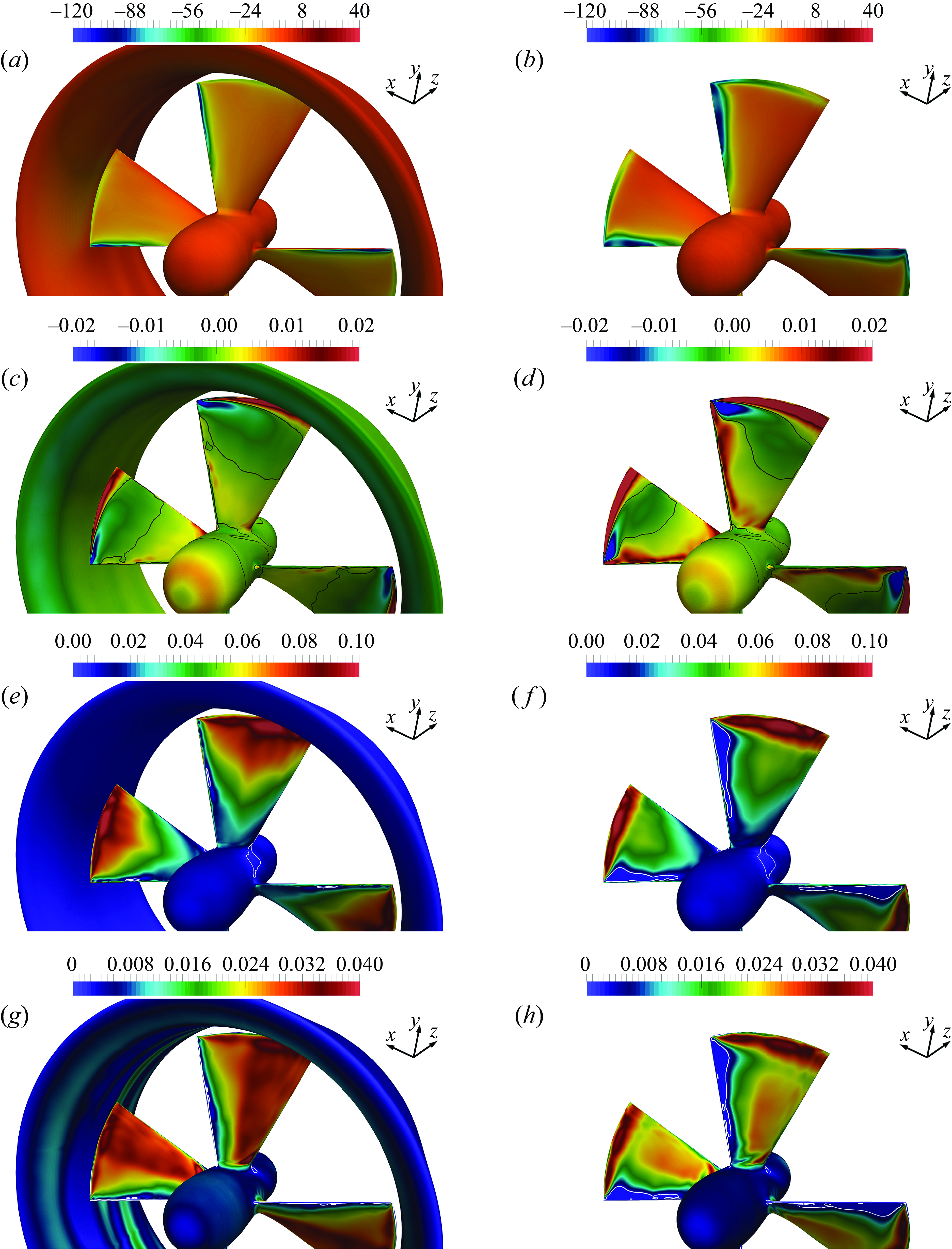
Contours of phase-averaged statistics on the suction side of the propellers: (a,b) $\widehat {c}_p$
, (c,d)
$\widehat {c}_p$
, (c,d) $\widehat {c}_{fr}$
, (e,f)
$\widehat {c}_{fr}$
, (e,f) $\widehat {c}_{f\vartheta }$
, (g,h)
$\widehat {c}_{f\vartheta }$
, (g,h) $\widehat {c}_{fz}$
. Isolines for locations of a 0 skin-friction coefficient on the propeller blades. Results for the ducted and conventional propellers are shown in the left and right panels, respectively.
$\widehat {c}_{fz}$
. Isolines for locations of a 0 skin-friction coefficient on the propeller blades. Results for the ducted and conventional propellers are shown in the left and right panels, respectively.
The grid discussed above is the ‘fine’ Eulerian grid, adopted to resolve both the conventional and ducted propellers. However, in order to verify grid convergence, the ducted propeller was also resolved on two additional grids, denoted as ‘medium’ and ‘coarse’. They were generated by decreasing the number of points across each coordinate direction of factors equal to about $\sqrt [3]{2}$
and
$\sqrt [3]{2}$
and $\sqrt [3]{2^2}$
, respectively. These grids consisted of
$\sqrt [3]{2^2}$
, respectively. These grids consisted of $676 \times 1630 \times 1630$
(1.8 billion) and
$676 \times 1630 \times 1630$
(1.8 billion) and $546 \times 1292 \times 1292$
(0.9 billion) points in the radial, azimuthal and axial directions. The following analysis of the results will provide comparisons across resolutions on both parameters of global performance and wake flow to demonstrate grid convergence. However, unless otherwise stated, all results reported in § 5 will refer to the computations conducted on the fine grid.
$546 \times 1292 \times 1292$
(0.9 billion) points in the radial, azimuthal and axial directions. The following analysis of the results will provide comparisons across resolutions on both parameters of global performance and wake flow to demonstrate grid convergence. However, unless otherwise stated, all results reported in § 5 will refer to the computations conducted on the fine grid.
Two Lagrangian grids were utilised to represent the immersed boundaries. The one discretizing the surface of the propeller consisted of about $178\,000$
triangles, while the duct was represented by using
$178\,000$
triangles, while the duct was represented by using $118\,000$
elements. These grids are shown in figure 4.
$118\,000$
elements. These grids are shown in figure 4.
The resolution in time was very fine, since tied to that in space by the stability requirements of the explicit Runge-Kutta scheme. All computations were carried out at a constant value of the Courant–Friedrichs–Lewy number, equal to 1.0. On the fine grid the average time step of the simulation of the ducted propeller was equivalent to $\Delta t U_\infty /D \approx 5.3 \times 10^{-5}$
. This resulted in about
$\Delta t U_\infty /D \approx 5.3 \times 10^{-5}$
. This resulted in about $5600$
time steps for the propeller to perform a full revolution. On the medium and coarse grids the average time steps were equal to
$5600$
time steps for the propeller to perform a full revolution. On the medium and coarse grids the average time steps were equal to $\Delta t U_\infty /D \approx 7.1 \times 10^{-5}$
and
$\Delta t U_\infty /D \approx 7.1 \times 10^{-5}$
and $\Delta t U_\infty /D \approx 8.9 \times 10^{-5}$
, respectively, which means that about
$\Delta t U_\infty /D \approx 8.9 \times 10^{-5}$
, respectively, which means that about $4200$
and
$4200$
and $3400$
time steps were required for each revolution of the propeller. The conventional propeller was simulated on the fine grid only. In this case the average time step was
$3400$
time steps were required for each revolution of the propeller. The conventional propeller was simulated on the fine grid only. In this case the average time step was $\Delta t U_\infty /D \approx 5.0 \times 10^{-5}$
, corresponding to
$\Delta t U_\infty /D \approx 5.0 \times 10^{-5}$
, corresponding to $6000$
time steps per revolution. All simulations were advanced in time for two flow-through times, with the purpose of developing the wake flow and achieving statistically steady conditions. Then, both time-averaged and phase-averaged statistics were computed at run time, including in the statistical sample all instantaneous realisations of the solution during a period of time equivalent to 10 revolutions of the propeller blades. In the following, time-averaged and phase-averaged statistics are indicated as
$6000$
time steps per revolution. All simulations were advanced in time for two flow-through times, with the purpose of developing the wake flow and achieving statistically steady conditions. Then, both time-averaged and phase-averaged statistics were computed at run time, including in the statistical sample all instantaneous realisations of the solution during a period of time equivalent to 10 revolutions of the propeller blades. In the following, time-averaged and phase-averaged statistics are indicated as $\overline {\varphi }$
and
$\overline {\varphi }$
and $\widehat {\varphi }$
, where
$\widehat {\varphi }$
, where $\varphi$
is a generic physical quantity. Fluctuations in time are denoted as
$\varphi$
is a generic physical quantity. Fluctuations in time are denoted as $\varphi $
′. Results for the time-averaged and phase-averaged turbulent kinetic energy are reported in § 5. These are defined as
$\varphi $
′. Results for the time-averaged and phase-averaged turbulent kinetic energy are reported in § 5. These are defined as
 \begin{align} \overline {k} = {1 \over 2} \left ( \overline {u'u'} + \overline {v'v'} + \overline {w'w'} \right ), \end{align}
 \begin{align} \widehat {k} = {1 \over 2} \left ( \widehat {u'u'} + \widehat {v'v'} + \widehat {w'w'} \right ), \end{align}
where $\overline {u'u'}$
,
$\overline {u'u'}$
, $\overline {v'v'}$
and
$\overline {v'v'}$
and $\overline {w'w'}$
are the time-averaged mean squares of the fluctuations in time of the radial, azimuthal and axial velocity components, respectively, while
$\overline {w'w'}$
are the time-averaged mean squares of the fluctuations in time of the radial, azimuthal and axial velocity components, respectively, while $\widehat {u'u'}$
,
$\widehat {u'u'}$
, $\widehat {v'v'}$
and
$\widehat {v'v'}$
and $\widehat {w'w'}$
are the phase-averaged ones. In addition, results for the turbulent shear stresses will be reported. Their time-averaged and phase-averaged statistics will be denoted as
$\widehat {w'w'}$
are the phase-averaged ones. In addition, results for the turbulent shear stresses will be reported. Their time-averaged and phase-averaged statistics will be denoted as $\overline {u'v'}$
,
$\overline {u'v'}$
, $\overline {u'w'}$
,
$\overline {u'w'}$
, $\overline {v'w'}$
and
$\overline {v'w'}$
and $\widehat {u'v'}$
,
$\widehat {u'v'}$
, $\widehat {u'w'}$
,
$\widehat {u'w'}$
, $\widehat {v'w'}$
, respectively.
$\widehat {v'w'}$
, respectively.
All simulations were carried out by parallel computing on distributed-memory supercomputers, by using an in-house-developed Fortran solver. In particular, the simulations on the fine, medium and coarse grids utilised $1024$
,
$1024$
, $814$
and
$814$
and $645$
cores, respectively. Domain decomposition was conducted in the axial direction, separating the overall problem in cylindrical subdomains. Communications between them were handled by calls to message passing interface (MPI) libraries. The overall cost of the simulations was equal to about 5 million CPU hours.
$645$
cores, respectively. Domain decomposition was conducted in the axial direction, separating the overall problem in cylindrical subdomains. Communications between them were handled by calls to message passing interface (MPI) libraries. The overall cost of the simulations was equal to about 5 million CPU hours.
5. Results
5.1. Parameters of global performance
The present study is focused on the comparison between the wake features of the ducted and conventional propellers. Nonetheless, parameters of global performance are given in this section for comparison with the DES computations reported by Gong et al. (Reference Gong, Guo, Zhao, Wu and Song2018) under the same conditions in an open-water set-up. For marine propellers, the major parameters of performance are the thrust coefficient, $K_T$
, the torque coefficient,
$K_T$
, the torque coefficient, $K_Q$
, and the efficiency of propulsion,
$K_Q$
, and the efficiency of propulsion, $\eta$
. It is worth noting that in the case of the ducted propeller the overall thrust coefficient is given by the sum of the thrust coefficients of the duct and the propeller,
$\eta$
. It is worth noting that in the case of the ducted propeller the overall thrust coefficient is given by the sum of the thrust coefficients of the duct and the propeller, $K_{Td}$
and
$K_{Td}$
and $K_{Tp}$
, respectively. All parameters are defined as
$K_{Tp}$
, respectively. All parameters are defined as
 \begin{equation} K_{Td} = {T_d \over \rho n^2 D^4},\qquad K_{Tp} = {T_p \over \rho n^2 D^4},\qquad K_Q = {Q \over \rho n^2 D^5}, \qquad \eta = {J (K_{Td} + K_{Tp}) \over 2\pi K_Q}. \end{equation}
In (5.1), $T_d$
and
$T_d$
and $T_p$
are the thrust forces generated by the duct and the propeller, respectively, while
$T_p$
are the thrust forces generated by the duct and the propeller, respectively, while $Q$
is the torque acting on the propeller blades.
$Q$
is the torque acting on the propeller blades.
Parameters of global performance of the ducted propeller.
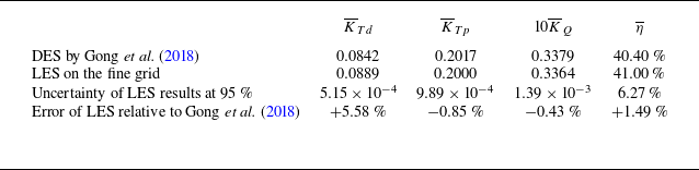
Parameters of global performance of the conventional propeller.

Table 1 provides a comparison of the present results on the ducted propeller against those by Gong et al. (Reference Gong, Guo, Zhao, Wu and Song2018). The results on the three fine, medium and coarse grids were also exploited to compute the uncertainty of LES results with a level of confidence of $95\,\%$
, based on the ‘factor of safety’ method by Xing & Stern (Reference Xing and Stern2010). The performance of the conventional propeller is summarised in table 2. It is worth mentioning that, for this case, the values of uncertainty are not available, since we carried out a grid sensitivity study only on the ducted propeller. This choice was tied to the need of saving computational resources, under the hypothesis that the flow physics is more challenging to reproduce when the propeller is operating within the nozzle. Therefore, we assumed that grid convergence is faster for the conventional propeller than for the ducted one. For both ducted and conventional propellers, the agreement between LES and DES is satisfactory. The relative error on the fine grid is the largest for the thrust generated by the nozzle, due to the smaller value of axial force acting on this component of the propeller, compared with its rotor. It is interesting to see that the presence of the duct has a dramatic impact on the performance. Compared with the conventional propeller, the overall thrust of the ducted propeller decreases by
$95\,\%$
, based on the ‘factor of safety’ method by Xing & Stern (Reference Xing and Stern2010). The performance of the conventional propeller is summarised in table 2. It is worth mentioning that, for this case, the values of uncertainty are not available, since we carried out a grid sensitivity study only on the ducted propeller. This choice was tied to the need of saving computational resources, under the hypothesis that the flow physics is more challenging to reproduce when the propeller is operating within the nozzle. Therefore, we assumed that grid convergence is faster for the conventional propeller than for the ducted one. For both ducted and conventional propellers, the agreement between LES and DES is satisfactory. The relative error on the fine grid is the largest for the thrust generated by the nozzle, due to the smaller value of axial force acting on this component of the propeller, compared with its rotor. It is interesting to see that the presence of the duct has a dramatic impact on the performance. Compared with the conventional propeller, the overall thrust of the ducted propeller decreases by $9.38\,\%$
in the results by Gong et al. (Reference Gong, Guo, Zhao, Wu and Song2018) and
$9.38\,\%$
in the results by Gong et al. (Reference Gong, Guo, Zhao, Wu and Song2018) and $12.11\,\%$
in our LES computations on the fine grid. Meanwhile, the reduction of the torque acting on the propeller blades is even more significant, equivalent to
$12.11\,\%$
in our LES computations on the fine grid. Meanwhile, the reduction of the torque acting on the propeller blades is even more significant, equivalent to $30.56\,\%$
and
$30.56\,\%$
and $32.88\,\%$
, respectively. As a result, a substantial increase of the efficiency of propulsion occurs (
$32.88\,\%$
, respectively. As a result, a substantial increase of the efficiency of propulsion occurs ( $30.50\,\%$
and
$30.50\,\%$
and $30.94\,\%$
, respectively), demonstrating the beneficial effect of the nozzle on the performance of the propeller. It is also worth mentioning that both loads acting on the duct and propellers are largely dominated by their pressure component. For the former, the viscous component provided a contribution equivalent to only about
$30.94\,\%$
, respectively), demonstrating the beneficial effect of the nozzle on the performance of the propeller. It is also worth mentioning that both loads acting on the duct and propellers are largely dominated by their pressure component. For the former, the viscous component provided a contribution equivalent to only about $1\,\%$
of the overall thrust. For the thrust and torque produced by the propeller blades, the viscous contribution was even below
$1\,\%$
of the overall thrust. For the thrust and torque produced by the propeller blades, the viscous contribution was even below $1\,\%$
. This is the reason why even less demanding methodologies may be assumed accurate enough as long as the only performance of propellers rather than their wake dynamics is required from computations. The following sections show that this dramatic change in performance is reflected in a substantial modification of the flow physics as well.
$1\,\%$
. This is the reason why even less demanding methodologies may be assumed accurate enough as long as the only performance of propellers rather than their wake dynamics is required from computations. The following sections show that this dramatic change in performance is reflected in a substantial modification of the flow physics as well.
5.2. Flow through the propellers
In this section the flow through the propellers is discussed by considering the pressure and skin-friction coefficients on the surface of their blades and nozzle from phase-averaged statistics of the solution. These coefficients are defined as
 \begin{equation} \widehat {c}_p={\widehat {p}-p_\infty \over 0.5 \rho U_\infty ^2},\qquad \widehat {c}_{f r}={\widehat {\tau }_{w r} \over 0.5 \rho U_\infty ^2},\qquad \widehat {c}_{f \vartheta }={\widehat {\tau }_{w \vartheta } \over 0.5 \rho U_\infty ^2},\qquad \widehat {c}_{f z}={\widehat {\tau }_{w z} \over 0.5 \rho U_\infty ^2}, \end{equation}
where $p_\infty$
is the free-stream pressure, while
$p_\infty$
is the free-stream pressure, while $\widehat {\tau }_{w r}$
,
$\widehat {\tau }_{w r}$
, $\widehat {\tau }_{w \vartheta }$
and
$\widehat {\tau }_{w \vartheta }$
and $\widehat {\tau }_{w z}$
are the phase-averaged values of the wall shear stresses in the radial, azimuthal and axial directions, respectively.
$\widehat {\tau }_{w z}$
are the phase-averaged values of the wall shear stresses in the radial, azimuthal and axial directions, respectively.
Figure 5 shows contours of the coefficients defined in (5.2) on the suction side of both ducted and conventional propellers. Isolines represent locations where the skin-friction coefficient is equal to 0. The most significant difference observed between the two propellers is the presence of a region of separation at the leading edge of the conventional propeller, identified by negative values of $\widehat {c}_{f \vartheta }$
and
$\widehat {c}_{f \vartheta }$
and $\widehat {c}_{f z}$
in figure 5(f,h). This separation is missing in the case of the ducted propeller, as shown in figure 5(e,g). The signature of this separation is visible in figure 5(b,d) as a wider region of low pressure and positive
$\widehat {c}_{f z}$
in figure 5(f,h). This separation is missing in the case of the ducted propeller, as shown in figure 5(e,g). The signature of this separation is visible in figure 5(b,d) as a wider region of low pressure and positive $\widehat {c}_{f r}$
in the vicinity of the leading edge, if compared with figure 5(a,c). It is also interesting to see that higher values of
$\widehat {c}_{f r}$
in the vicinity of the leading edge, if compared with figure 5(a,c). It is also interesting to see that higher values of $\widehat {c}_{f r}$
are achieved at the tip of the blades of the conventional propeller (figure 5
d), if compared with the ducted one (figure 5
c). They are due to the vortices produced by the cross-flow between pressure and suction sides of the blades. They are more intense for the conventional propeller, which is more loaded. The lower load on the blades of the ducted propeller can be explained by considering the acceleration of the incoming flow by its nozzle. This acceleration results in a modification of the actual advance coefficient experienced by the propeller blades, which becomes higher, equivalent to lower loads. Therefore, the blades of the ducted propeller are operating at smaller incidence angles and lower loads, if compared with those of the conventional propeller, producing less intense vortices at their tip and less separation on their suction side. This is the reason why typically ducted propellers display flatter characteristic curves, which means they are able to keep a higher efficiency at lower values of nominal advance coefficient, if compared with propellers without a nozzle.
$\widehat {c}_{f r}$
are achieved at the tip of the blades of the conventional propeller (figure 5
d), if compared with the ducted one (figure 5
c). They are due to the vortices produced by the cross-flow between pressure and suction sides of the blades. They are more intense for the conventional propeller, which is more loaded. The lower load on the blades of the ducted propeller can be explained by considering the acceleration of the incoming flow by its nozzle. This acceleration results in a modification of the actual advance coefficient experienced by the propeller blades, which becomes higher, equivalent to lower loads. Therefore, the blades of the ducted propeller are operating at smaller incidence angles and lower loads, if compared with those of the conventional propeller, producing less intense vortices at their tip and less separation on their suction side. This is the reason why typically ducted propellers display flatter characteristic curves, which means they are able to keep a higher efficiency at lower values of nominal advance coefficient, if compared with propellers without a nozzle.
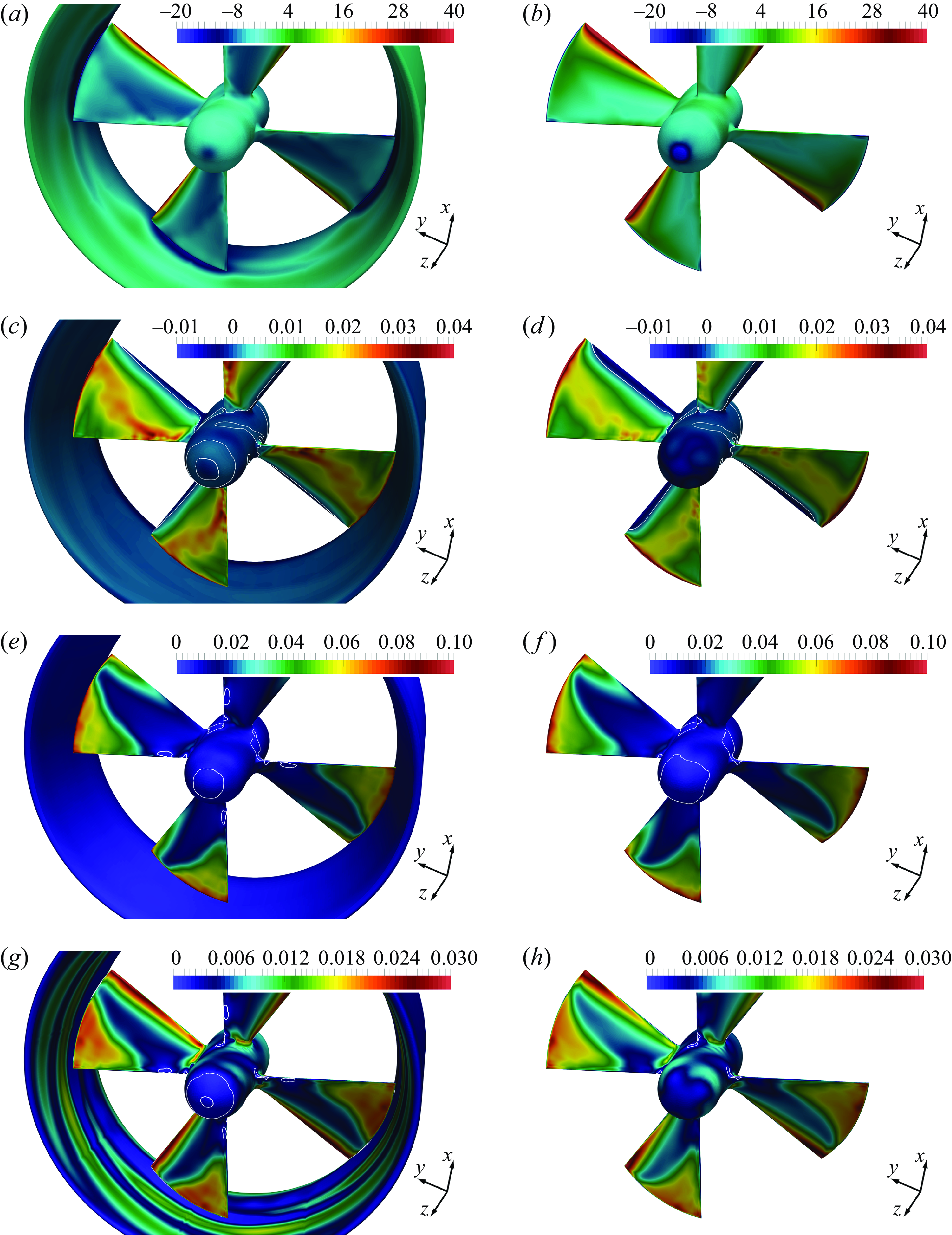
Contours of phase-averaged statistics on the pressure side of the propellers: (a,b) $\widehat {c}_p$
, (c,d)
$\widehat {c}_p$
, (c,d) $\widehat {c}_{fr}$
, (e,f)
$\widehat {c}_{fr}$
, (e,f) $\widehat {c}_{f\vartheta }$
, (g,h)
$\widehat {c}_{f\vartheta }$
, (g,h) $\widehat {c}_{fz}$
. Isolines for locations of a 0 skin-friction coefficient on the propeller blades. Results for the ducted and conventional propellers are shown in the left and right panels, respectively.
$\widehat {c}_{fz}$
. Isolines for locations of a 0 skin-friction coefficient on the propeller blades. Results for the ducted and conventional propellers are shown in the left and right panels, respectively.
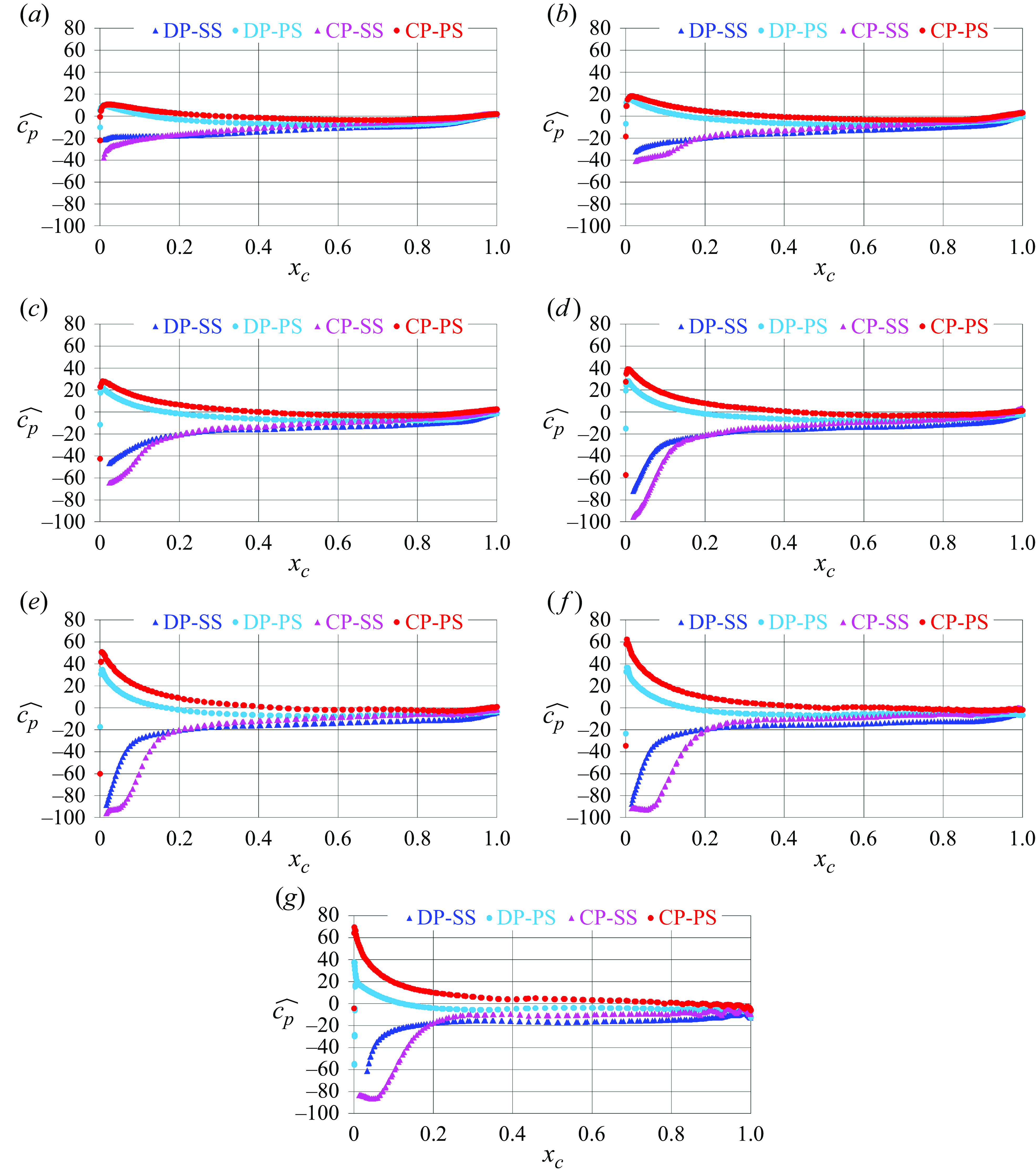
Distribution of the phase-averaged pressure coefficient on the suction side (SS) and pressure side (PS) of the propeller blades: (a) $r/D=0.15$
, (b)
$r/D=0.15$
, (b) $r/D=0.20$
, (c)
$r/D=0.20$
, (c) $r/D=0.25$
, (d)
$r/D=0.25$
, (d) $r/D=0.30$
, (e)
$r/D=0.30$
, (e) $r/D=0.35$
, (f)
$r/D=0.35$
, (f) $r/D=0.40$
, (g)
$r/D=0.40$
, (g) $r/D=0.45$
. Comparison between the ducted propeller (DP) and conventional propeller (CP).
$r/D=0.45$
. Comparison between the ducted propeller (DP) and conventional propeller (CP).
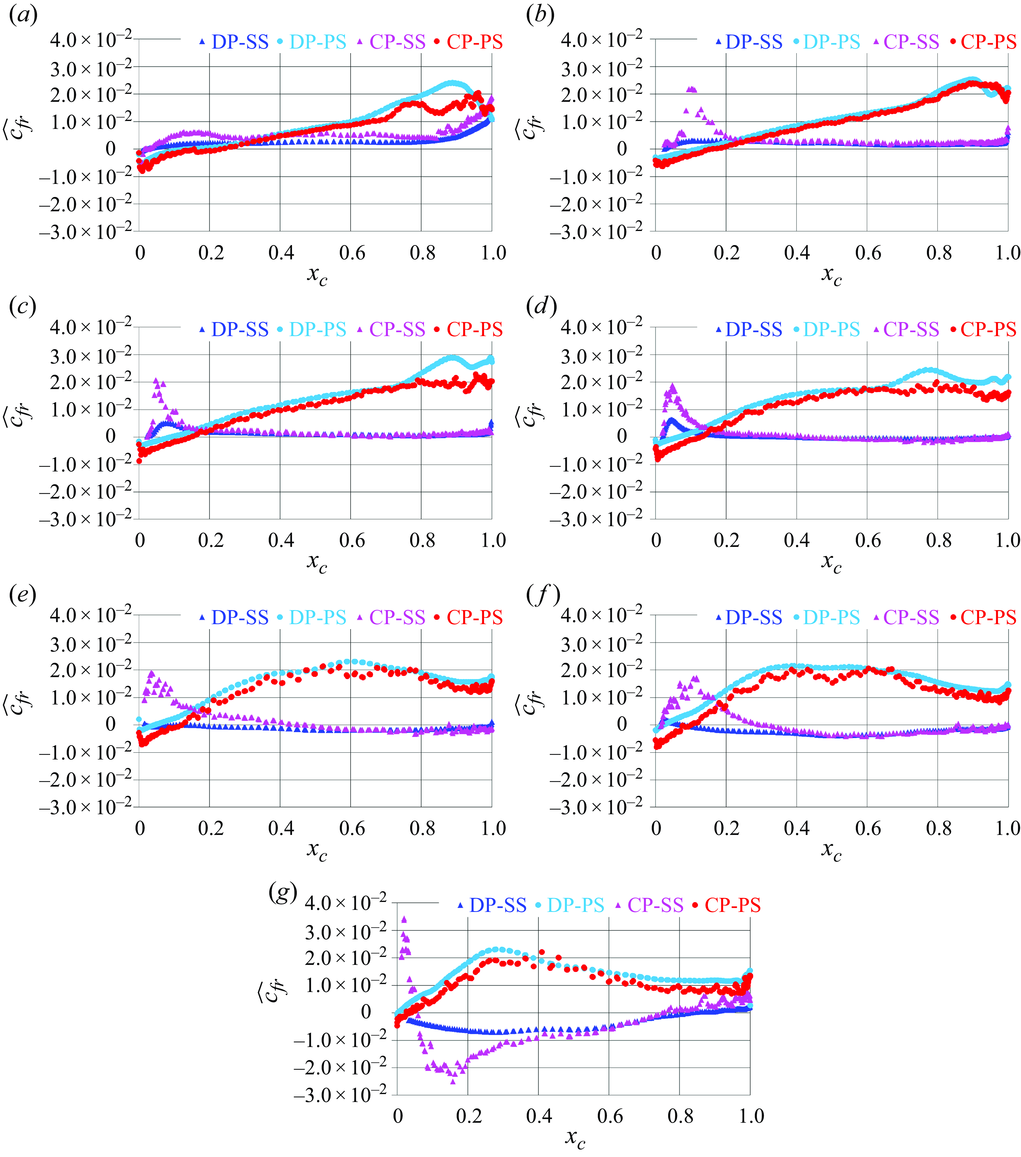
Distribution of the phase-averaged radial skin-friction coefficient on the suction side (SS) and pressure side (PS) of the propeller blades: (a) $r/D=0.15$
, (b)
$r/D=0.15$
, (b) $r/D=0.20$
, (c)
$r/D=0.20$
, (c) $r/D=0.25$
, (d)
$r/D=0.25$
, (d) $r/D=0.30$
, (e)
$r/D=0.30$
, (e) $r/D=0.35$
, (f)
$r/D=0.35$
, (f) $r/D=0.40$
, (g)
$r/D=0.40$
, (g) $r/D=0.45$
. Comparison between the ducted propeller (DP) and conventional propeller (CP).
$r/D=0.45$
. Comparison between the ducted propeller (DP) and conventional propeller (CP).
The differences between the two propellers are less obvious on their pressure side, as shown in the contours of figure 6. The most significant deviations between them affect the pressure coefficient. The blades of the conventional propeller are more loaded. Therefore, the values of $\widehat {c}_{p}$
in figure 6(b) are higher than those in figure 6(a). The stronger minimum of pressure at the tail of the end cap of the conventional propeller is also the signature of a more intense hub vortex, in line with the higher load experienced by this propeller. For the components of the skin-friction coefficient, the qualitative agreement between the two propellers is closer than on the suction side, since on the pressure side the chordwise pressure gradient is favourable and large separation phenomena are missing in both cases. Outward radial flows are produced across the span of the propeller blades. The highest levels of stresses in the azimuthal and axial directions are achieved at the outermost radial coordinates for both propellers.
$\widehat {c}_{p}$
in figure 6(b) are higher than those in figure 6(a). The stronger minimum of pressure at the tail of the end cap of the conventional propeller is also the signature of a more intense hub vortex, in line with the higher load experienced by this propeller. For the components of the skin-friction coefficient, the qualitative agreement between the two propellers is closer than on the suction side, since on the pressure side the chordwise pressure gradient is favourable and large separation phenomena are missing in both cases. Outward radial flows are produced across the span of the propeller blades. The highest levels of stresses in the azimuthal and axial directions are achieved at the outermost radial coordinates for both propellers.
More details for the distribution of the pressure coefficient on the propeller blades are given in figure 7, where it is shown as a function of the chordwise coordinate, $x_c$
, at several spanwise locations, from
$x_c$
, at several spanwise locations, from $r/D=0.15$
to
$r/D=0.15$
to $r/D=0.45$
. The gap of the values of
$r/D=0.45$
. The gap of the values of $\widehat {c}_p$
between the pressure and suction sides is larger on the blades of the conventional propeller. As discussed above, the acceleration of the flow by the nozzle increases the actual advance coefficient experienced by the rotor of the ducted propeller, resulting in lower levels of load, compensated by the thrust produced by the nozzle itself. For both propellers, the load on their blades grows from inner to outer radial coordinates. On the pressure side the values of
$\widehat {c}_p$
between the pressure and suction sides is larger on the blades of the conventional propeller. As discussed above, the acceleration of the flow by the nozzle increases the actual advance coefficient experienced by the rotor of the ducted propeller, resulting in lower levels of load, compensated by the thrust produced by the nozzle itself. For both propellers, the load on their blades grows from inner to outer radial coordinates. On the pressure side the values of $\widehat {c}_p$
are higher on the blades of the conventional propeller, but their distributions are similar between the two cases. In contrast, their suction sides also show a different distribution in the vicinity of the leading edge, especially at the outermost radial coordinates. A wider region of low pressure is produced in the case of the conventional propeller, which is the signature of separation phenomena, missing instead on the less-loaded blades of the ducted propeller.
$\widehat {c}_p$
are higher on the blades of the conventional propeller, but their distributions are similar between the two cases. In contrast, their suction sides also show a different distribution in the vicinity of the leading edge, especially at the outermost radial coordinates. A wider region of low pressure is produced in the case of the conventional propeller, which is the signature of separation phenomena, missing instead on the less-loaded blades of the ducted propeller.
Profiles of the radial component of the skin-friction coefficient are reported in figure 8. In this case, values are very close between ducted and conventional propellers on the pressure side: positive radial flows are produced, increasing from the leading edge towards the trailing edge, although this trend diminishes moving from inner to outer radial coordinates. In general, radial flows are almost missing on the suction side of the blades. Again, the exception is represented by the region in the vicinity of the leading edge of the blades of the conventional propeller, where separation results in the onset of a peak of positive values of $\widehat {c}_{fr}$
. In the vicinity of the tip of the blades of the conventional propeller the behaviour of the skin-friction coefficient becomes more complex, as shown in figure 8(g). The positive peak at the leading edge is followed by a wide region of negative values, which is attributable to the onset of a strong tip vortex. In contrast, in the case of the ducted propeller the tip leakage vortex is weaker and its influence on the distribution of
$\widehat {c}_{fr}$
. In the vicinity of the tip of the blades of the conventional propeller the behaviour of the skin-friction coefficient becomes more complex, as shown in figure 8(g). The positive peak at the leading edge is followed by a wide region of negative values, which is attributable to the onset of a strong tip vortex. In contrast, in the case of the ducted propeller the tip leakage vortex is weaker and its influence on the distribution of $\widehat {c}_{fr}$
is not able to extend up to the radial coordinate
$\widehat {c}_{fr}$
is not able to extend up to the radial coordinate $r/D=0.45$
of figure 8(g).
$r/D=0.45$
of figure 8(g).
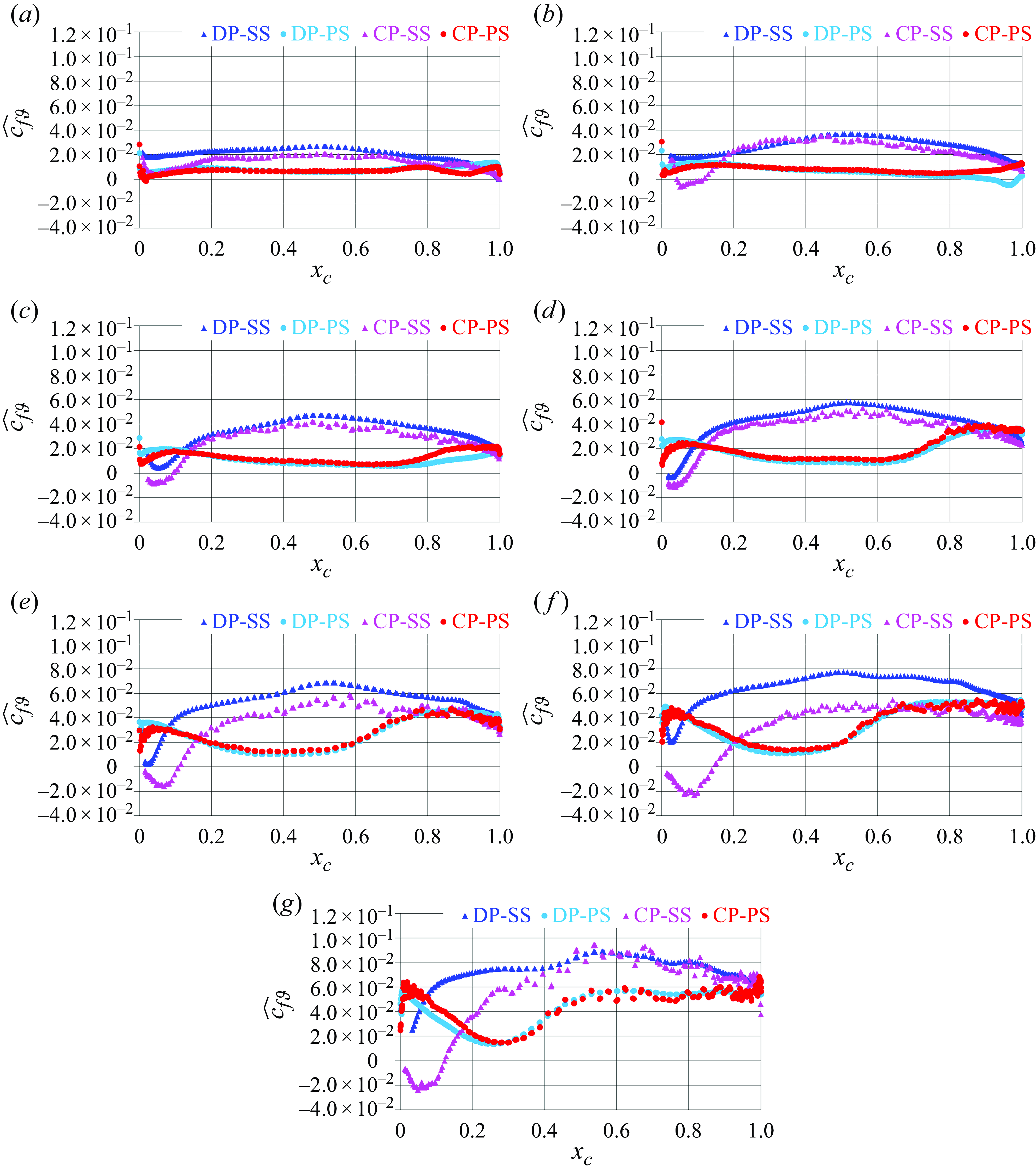
Distribution of the phase-averaged azimuthal skin-friction coefficient on the suction side (SS) and pressure side (PS) of the propeller blades: (a) $r/D=0.15$
, (b)
$r/D=0.15$
, (b) $r/D=0.20$
, (c)
$r/D=0.20$
, (c) $r/D=0.25$
, (d)
$r/D=0.25$
, (d) $r/D=0.30$
, (e)
$r/D=0.30$
, (e) $r/D=0.35$
, (f)
$r/D=0.35$
, (f) $r/D=0.40$
, (g)
$r/D=0.40$
, (g) $r/D=0.45$
. Comparison between the ducted propeller (DP) and conventional propeller (CP).
$r/D=0.45$
. Comparison between the ducted propeller (DP) and conventional propeller (CP).
Distribution of the phase-averaged streamwise skin-friction coefficient on the suction side (SS) and pressure side (PS) of the propeller blades: (a) $r/D=0.15$
, (b)
$r/D=0.15$
, (b) $r/D=0.20$
, (c)
$r/D=0.20$
, (c) $r/D=0.25$
, (d)
$r/D=0.25$
, (d) $r/D=0.30$
, (e)
$r/D=0.30$
, (e) $r/D=0.35$
, (f)
$r/D=0.35$
, (f) $r/D=0.40$
, (g)
$r/D=0.40$
, (g) $r/D=0.45$
. Comparison between the ducted propeller (DP) and conventional propeller (CP).
$r/D=0.45$
. Comparison between the ducted propeller (DP) and conventional propeller (CP).
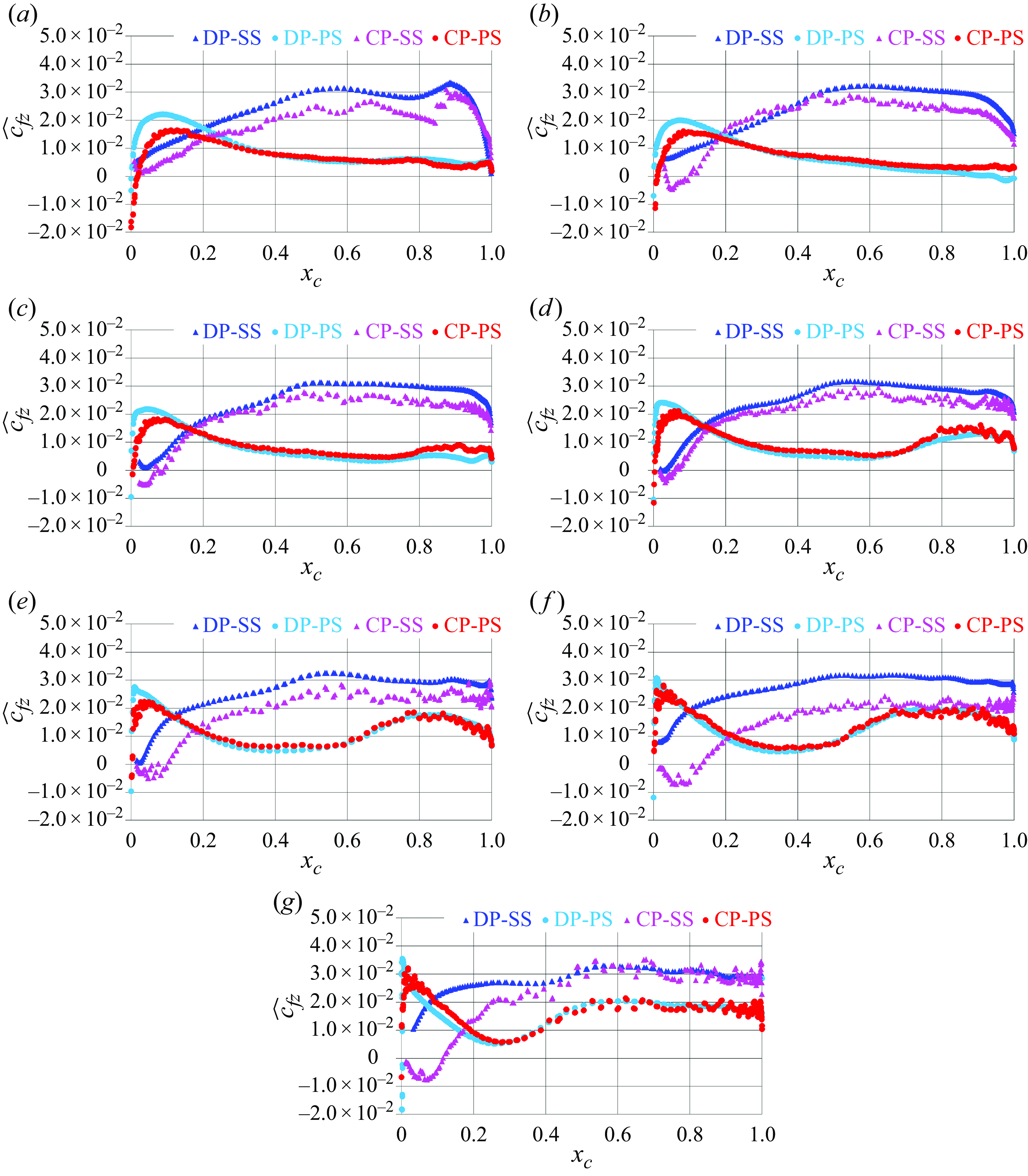
The azimuthal component of the skin-friction coefficient also shows similar values on the pressure side of the blades of the two propellers, as illustrated in figure 9. On the suction side higher values are achieved, growing from inner towards outer radial coordinates, and again the deviations between ducted and conventional propellers are more significant than on the pressure side. Actually, at the innermost radial coordinates (figure 9 a–d) they remain limited to the region just downstream of the leading edge, due to the separation affecting the blades of the conventional propeller and missing on the blades of the ducted propeller. At downstream chordwise coordinates the skin friction achieves slightly higher levels across the blades of the ducted propeller, as a result of the acceleration experienced by the flow within the nozzle. The extent of the leading edge separation on the blades of the conventional propeller grows at the outermost radial coordinates (figure 9 e–g), resulting in a wider region of negative values and significantly lower levels of the skin-friction coefficient, compared with the ducted propeller, even downstream of reattachment. The results for the streamwise component of the skin-friction coefficient, illustrated in figure 10, are qualitatively similar to those in figure 9, although lower levels are achieved, since the major component of the velocity of the flow, relative to the propeller blades, is the azimuthal one, rather than the streamwise one. However, it is interesting to see that higher values of skin friction occur across the blades of the ducted propeller not only on their suction side but also in the positive peak on the pressure side at their leading edge, again as a result of the acceleration of the flow promoted by the presence of the nozzle.
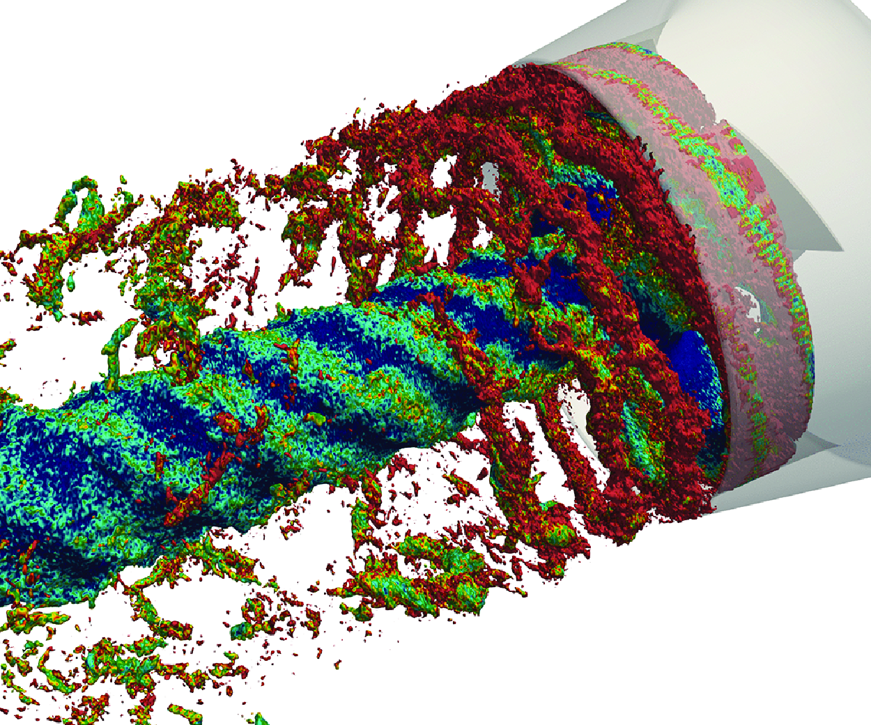
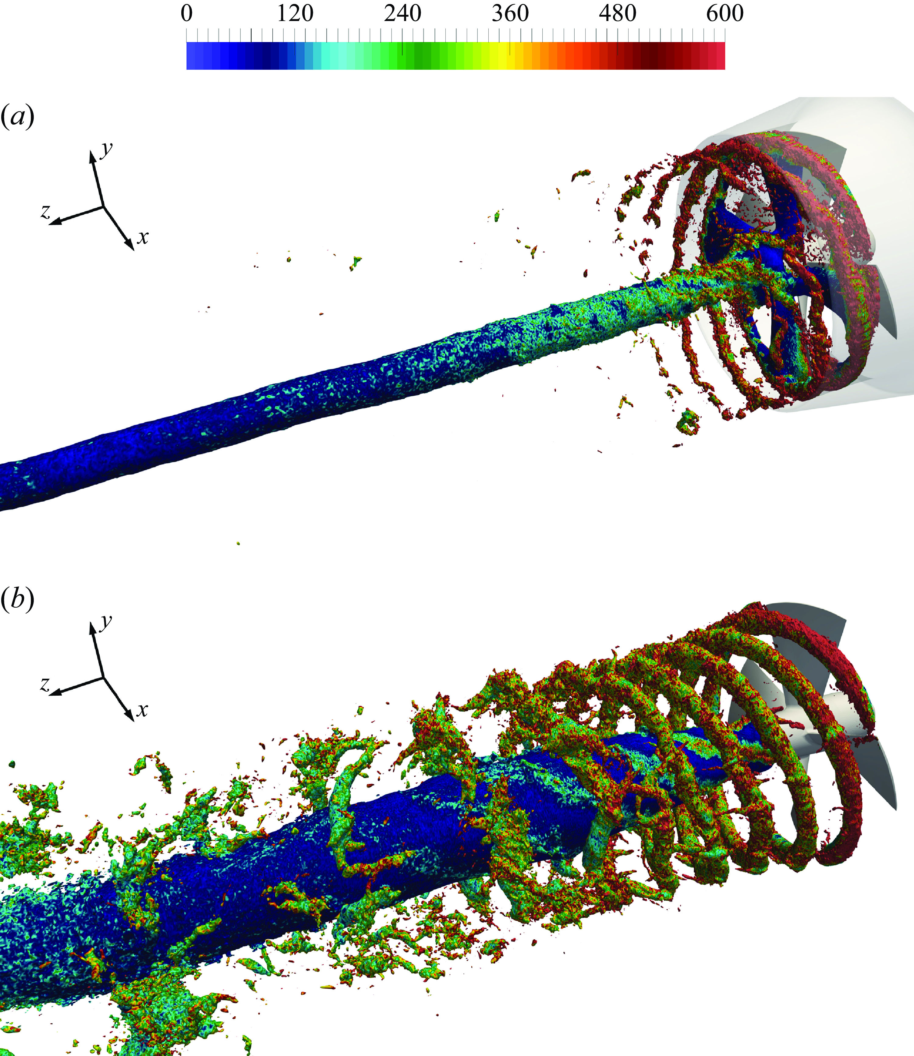
Isosurfaces of the pressure coefficient ( $c_p=-1.6$
) from instantaneous realisations of the solution. Contours of vorticity magnitude, scaled by
$c_p=-1.6$
) from instantaneous realisations of the solution. Contours of vorticity magnitude, scaled by $U_\infty /D$
. Comparison between (a) ducted and (b) conventional propellers.
$U_\infty /D$
. Comparison between (a) ducted and (b) conventional propellers.
Isosurfaces of the pressure coefficient ( $c_p=-0.4$
) from instantaneous realisations of the solution of the ducted propeller on the (a) fine, (b) medium and (c) coarse grids. Contours of vorticity magnitude, scaled by
$c_p=-0.4$
) from instantaneous realisations of the solution of the ducted propeller on the (a) fine, (b) medium and (c) coarse grids. Contours of vorticity magnitude, scaled by $U_\infty /D$
.
$U_\infty /D$
.
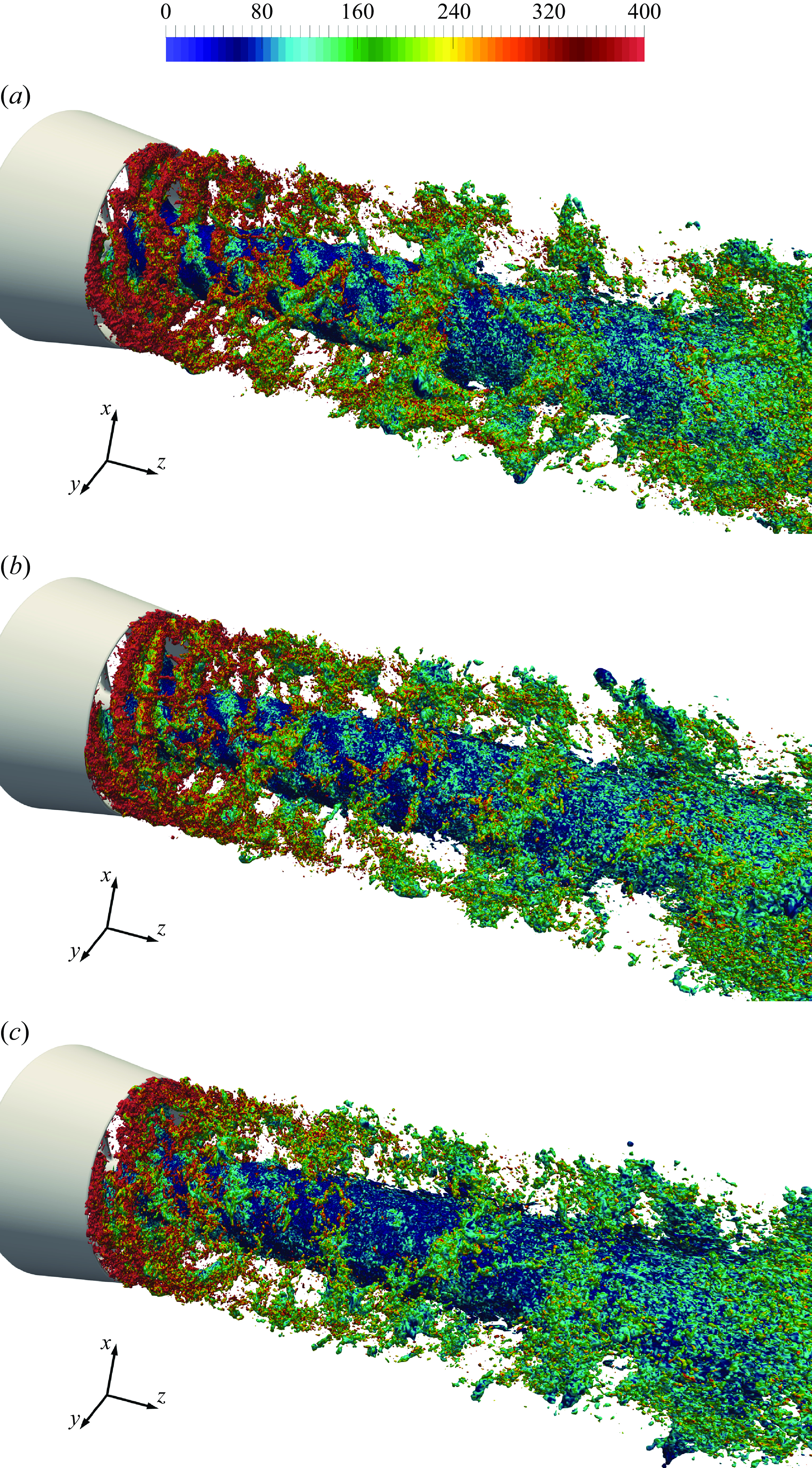
Isosurfaces of the second invariant of the velocity gradient tensor ( $\mathcal {Q}\text{-criterion}$
) from phase-averaged statistics of the solution (
$\mathcal {Q}\text{-criterion}$
) from phase-averaged statistics of the solution ( $\widehat {\mathcal {Q}}D^2/U_\infty ^2=100$
). Contours of vorticity magnitude, scaled by
$\widehat {\mathcal {Q}}D^2/U_\infty ^2=100$
). Contours of vorticity magnitude, scaled by $U_\infty /D$
. Comparison between (a) ducted and (b) conventional propellers.
$U_\infty /D$
. Comparison between (a) ducted and (b) conventional propellers.
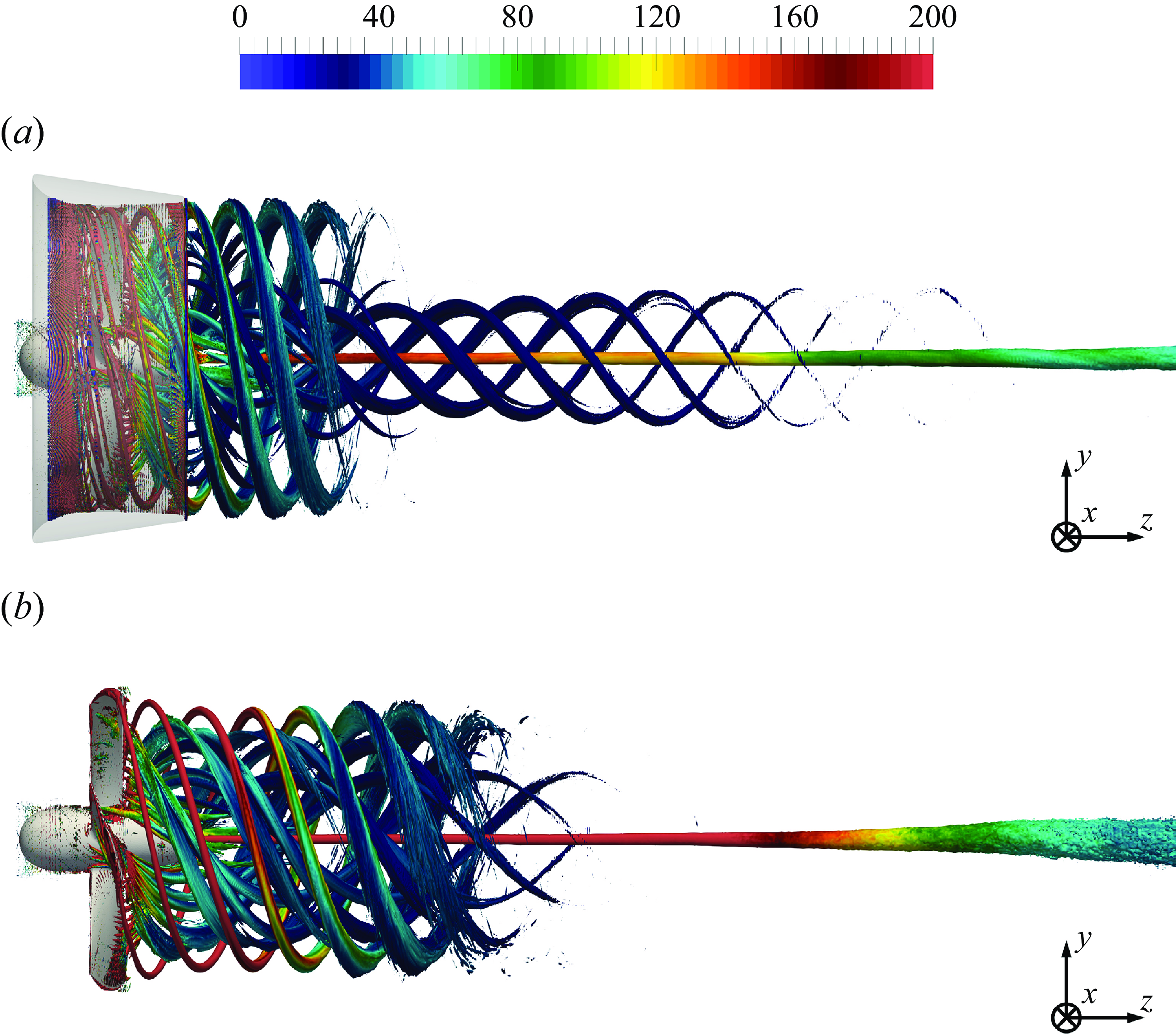
5.3. Overview of the major wake structures
Figure 11 shows isosurfaces of the pressure coefficient, coloured by vorticity magnitude, from instantaneous realisations of the solution. The dramatic change of the topology of the wake flow is evident. The tip vortices shed by the conventional propeller are more intense than the tip leakage vortices shed by the ducted propeller. They also keep coherent across farther downstream distances. Therefore, the presence of the duct results in tip leakage vortices that are weaker and experience a faster instability, in comparison with the tip vortices shed by the conventional propeller.
The particular value for $c_p$
in figure 11 has the purpose of illustrating the comparison between the wakes of the ducted and conventional propellers. The breakup of the tip leakage vortices into smaller structures is shown in better detail across grid resolutions in figure 12, where a smaller value of
$c_p$
in figure 11 has the purpose of illustrating the comparison between the wakes of the ducted and conventional propellers. The breakup of the tip leakage vortices into smaller structures is shown in better detail across grid resolutions in figure 12, where a smaller value of $c_p$
(in magnitude) is considered for isolating the structures populating the flow further away from the propeller. It is demonstrated that the adopted computational grid is able to resolve the smaller structures resulting from the instability of the tip leakage vortices. It is worth recalling that the ducted and conventional propellers were resolved on the same computational grid. Therefore, the dramatic change of the flow physics observed in figure 11 is not dependent on grid resolution, as also demonstrated in figure 12. While in figure 12 some deviations on the coherence of the tip leakage vortices are visible between the coarse and medium grids, the agreement between medium and fine grids is good. More detailed, quantitative comparisons across resolutions will be provided later through the statistics of the flow.
$c_p$
(in magnitude) is considered for isolating the structures populating the flow further away from the propeller. It is demonstrated that the adopted computational grid is able to resolve the smaller structures resulting from the instability of the tip leakage vortices. It is worth recalling that the ducted and conventional propellers were resolved on the same computational grid. Therefore, the dramatic change of the flow physics observed in figure 11 is not dependent on grid resolution, as also demonstrated in figure 12. While in figure 12 some deviations on the coherence of the tip leakage vortices are visible between the coarse and medium grids, the agreement between medium and fine grids is good. More detailed, quantitative comparisons across resolutions will be provided later through the statistics of the flow.
Isosurfaces of the second invariant of the velocity gradient tensor ( $\mathcal {Q}\text{-criterion}$
) from phase-averaged statistics of the solution (
$\mathcal {Q}\text{-criterion}$
) from phase-averaged statistics of the solution ( $\widehat {\mathcal {Q}}D^2/U_\infty ^2=100$
). Contours of vorticity magnitude, scaled by
$\widehat {\mathcal {Q}}D^2/U_\infty ^2=100$
). Contours of vorticity magnitude, scaled by $U_\infty /D$
. Isosurfaces at the outer boundary of the wake removed for visibility of the inner vortices. Comparison between (a) ducted and (b) conventional propellers.
$U_\infty /D$
. Isosurfaces at the outer boundary of the wake removed for visibility of the inner vortices. Comparison between (a) ducted and (b) conventional propellers.

Visualisations from phase-averaged statistics of the wake flow are provided in figure 13 ( $\mathcal {Q}\text{-criterion}$
by Jeong & Hussain Reference Jeong and Hussain1995), where again the comparison deals with the cases of the ducted and conventional propellers. Phase averages are useful to isolate the coherent structures in the wake of the propeller as long as they keep synchronised with its rotation. Their instability results in their diffusion in the phase-averaged fields. This phenomenon occurs earlier for the tip leakage vortices shed by the ducted propeller, in comparison with the tip vortices shed by the conventional propeller. In both cases the hub vortex populating the wake axis is able to keep its coherence further downstream within the streamwise extent of the computational domain. Interestingly, additional helical structures populate the wake core. The comparison between the two panels of figure 13 shows that they differ between the ducted and conventional propellers, pointing out that the differences between their wake systems are not limited to the outer radii. The presence of the duct is able to modify the flow downstream of the propeller even at inner radial coordinates. For instance, the wake of the ducted propeller is populated by stronger, more long standing helical structures near the root of the blades, in comparison with the wake of the conventional propeller, whose helical vortices are stronger at outer radial coordinates. This is more clear in figure 14, where the vortices shed from the tip of the propeller blades were removed, for visibility of the vortices populating the wake core. These differences in the wake of the two propellers can be explained by considering their different inflow conditions. The presence of the nozzle results in higher values of streamwise velocity at the inlet of the propeller. This change produces a modification of the velocity of the flow, relative to the propeller blades, and thus, a modification of its incidence angle and distribution of the load across the span of the blades. This is the reason why changes in the coherent structures shed by the propeller affect not only their tip, extending to the whole range of radial coordinates. In particular, since the incidence angle experienced by the propeller blades is the result of the composition between the streamwise velocity of the flow and the azimuthal velocity of the propeller blades, the modification of the incidence angle of the flow is especially significant at the innermost radial coordinates. The acceleration of the incoming flow was verified to be rather uniform across radial coordinates. Therefore, the increase of the streamwise velocity relative to the azimuthal velocity is the largest at the root of the blades, because there their azimuthal velocity is the lowest. Meanwhile, it should be noted that the vortices shed at the innermost spanwise coordinates of the blades experience interaction with the hub vortex, which is more intense downstream of the more loaded conventional propeller, affecting a wider region around the wake axis, as shown by the instantaneous visualisations in figure 11. This interaction promotes a faster instability of the vortices shed at the innermost spanwise coordinates by the conventional propeller, compared with the ducted one. We indeed verified the onset of similar structures near the root of the two propellers. However, these vortices lose more quickly their coherence downstream of the conventional propeller. This result is illustrated in better detail in figure 15, where phase-averaged flow fields are shown, removing again the structures at the outermost radial coordinates for visibility of the innermost ones. Differences affect all spanwise coordinates, due to the different load conditions experienced by the blades of the two propellers. However, the innermost vortices are not in general more intense in the case of the ducted propeller, as demonstrated by both isosurfaces of
$\mathcal {Q}\text{-criterion}$
by Jeong & Hussain Reference Jeong and Hussain1995), where again the comparison deals with the cases of the ducted and conventional propellers. Phase averages are useful to isolate the coherent structures in the wake of the propeller as long as they keep synchronised with its rotation. Their instability results in their diffusion in the phase-averaged fields. This phenomenon occurs earlier for the tip leakage vortices shed by the ducted propeller, in comparison with the tip vortices shed by the conventional propeller. In both cases the hub vortex populating the wake axis is able to keep its coherence further downstream within the streamwise extent of the computational domain. Interestingly, additional helical structures populate the wake core. The comparison between the two panels of figure 13 shows that they differ between the ducted and conventional propellers, pointing out that the differences between their wake systems are not limited to the outer radii. The presence of the duct is able to modify the flow downstream of the propeller even at inner radial coordinates. For instance, the wake of the ducted propeller is populated by stronger, more long standing helical structures near the root of the blades, in comparison with the wake of the conventional propeller, whose helical vortices are stronger at outer radial coordinates. This is more clear in figure 14, where the vortices shed from the tip of the propeller blades were removed, for visibility of the vortices populating the wake core. These differences in the wake of the two propellers can be explained by considering their different inflow conditions. The presence of the nozzle results in higher values of streamwise velocity at the inlet of the propeller. This change produces a modification of the velocity of the flow, relative to the propeller blades, and thus, a modification of its incidence angle and distribution of the load across the span of the blades. This is the reason why changes in the coherent structures shed by the propeller affect not only their tip, extending to the whole range of radial coordinates. In particular, since the incidence angle experienced by the propeller blades is the result of the composition between the streamwise velocity of the flow and the azimuthal velocity of the propeller blades, the modification of the incidence angle of the flow is especially significant at the innermost radial coordinates. The acceleration of the incoming flow was verified to be rather uniform across radial coordinates. Therefore, the increase of the streamwise velocity relative to the azimuthal velocity is the largest at the root of the blades, because there their azimuthal velocity is the lowest. Meanwhile, it should be noted that the vortices shed at the innermost spanwise coordinates of the blades experience interaction with the hub vortex, which is more intense downstream of the more loaded conventional propeller, affecting a wider region around the wake axis, as shown by the instantaneous visualisations in figure 11. This interaction promotes a faster instability of the vortices shed at the innermost spanwise coordinates by the conventional propeller, compared with the ducted one. We indeed verified the onset of similar structures near the root of the two propellers. However, these vortices lose more quickly their coherence downstream of the conventional propeller. This result is illustrated in better detail in figure 15, where phase-averaged flow fields are shown, removing again the structures at the outermost radial coordinates for visibility of the innermost ones. Differences affect all spanwise coordinates, due to the different load conditions experienced by the blades of the two propellers. However, the innermost vortices are not in general more intense in the case of the ducted propeller, as demonstrated by both isosurfaces of $\mathcal {Q}$
and contours of the vorticity magnitude. Meanwhile, those shed by the conventional propeller experience a faster diffusion. It is also interesting to see that the phase-averaged signature of the root vortices is lost very quickly downstream of both propellers, which means that actually the helical structures seen in the wake of the ducted propeller at inner radial coordinates in figure 14 are not those originating from the root of its blades. Instead, they come from spanwise coordinates further away from their root.
$\mathcal {Q}$
and contours of the vorticity magnitude. Meanwhile, those shed by the conventional propeller experience a faster diffusion. It is also interesting to see that the phase-averaged signature of the root vortices is lost very quickly downstream of both propellers, which means that actually the helical structures seen in the wake of the ducted propeller at inner radial coordinates in figure 14 are not those originating from the root of its blades. Instead, they come from spanwise coordinates further away from their root.
5.4. Evolution of the tip leakage vortices within the nozzle
In this section the evolution of the tip leakage vortices within the nozzle is studied by relying on the vortex core analysis. Comparisons with similar results for the tip vortices shed by the conventional propeller are also reported. In figure 16 a phase-averaged visualisation of the tip and tip leakage vortices is shown, which are isolated by means of isosurfaces of $\widehat {\mathcal {Q}}D^2/U_\infty ^2=10\,000$
. In the same visualisations, cross-sections of one of the vortices are indicated. They were generated by cutting the core of the vortex at azimuthal planes evenly spaced of
$\widehat {\mathcal {Q}}D^2/U_\infty ^2=10\,000$
. In the same visualisations, cross-sections of one of the vortices are indicated. They were generated by cutting the core of the vortex at azimuthal planes evenly spaced of $\pi /8$
radians. The phase-averaged statistics at the core of the vortex are reported below.
$\pi /8$
radians. The phase-averaged statistics at the core of the vortex are reported below.
Isosurfaces of the second invariant of the velocity gradient tensor ( $\mathcal {Q}\text{-criterion}$
) from phase-averaged statistics of the solution (
$\mathcal {Q}\text{-criterion}$
) from phase-averaged statistics of the solution ( $\widehat {\mathcal {Q}}D^2/U_\infty ^2=1000$
). Contours of vorticity magnitude, scaled by
$\widehat {\mathcal {Q}}D^2/U_\infty ^2=1000$
). Contours of vorticity magnitude, scaled by $U_\infty /D$
. Isosurfaces at the outer boundary of the wake removed for visibility of the inner vortices. Comparison between (a) ducted and (b) conventional propellers.
$U_\infty /D$
. Isosurfaces at the outer boundary of the wake removed for visibility of the inner vortices. Comparison between (a) ducted and (b) conventional propellers.
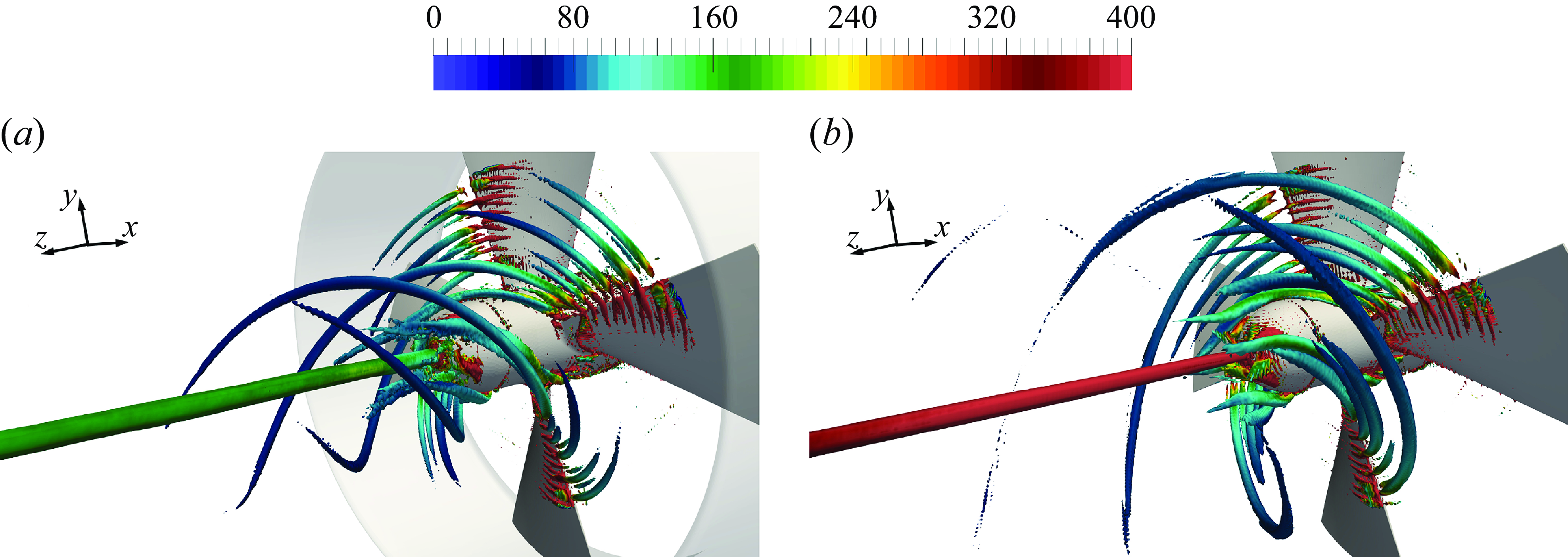
Isosurfaces of the second invariant of the velocity gradient tensor ( $\mathcal {Q}\text{-criterion}$
) from phase-averaged statistics of the solution (
$\mathcal {Q}\text{-criterion}$
) from phase-averaged statistics of the solution ( $\widehat {\mathcal {Q}}D^2/U_\infty ^2=10\,000$
). Contours of azimuthal vorticity, scaled by
$\widehat {\mathcal {Q}}D^2/U_\infty ^2=10\,000$
). Contours of azimuthal vorticity, scaled by $U_\infty /D$
. Representation of cross-sections of tip leakage and tip vortices shed by the (a) ducted and (b) conventional propellers, respectively, cut by meridian planes evenly spaced of
$U_\infty /D$
. Representation of cross-sections of tip leakage and tip vortices shed by the (a) ducted and (b) conventional propellers, respectively, cut by meridian planes evenly spaced of $\pi /8$
radians.
$\pi /8$
radians.
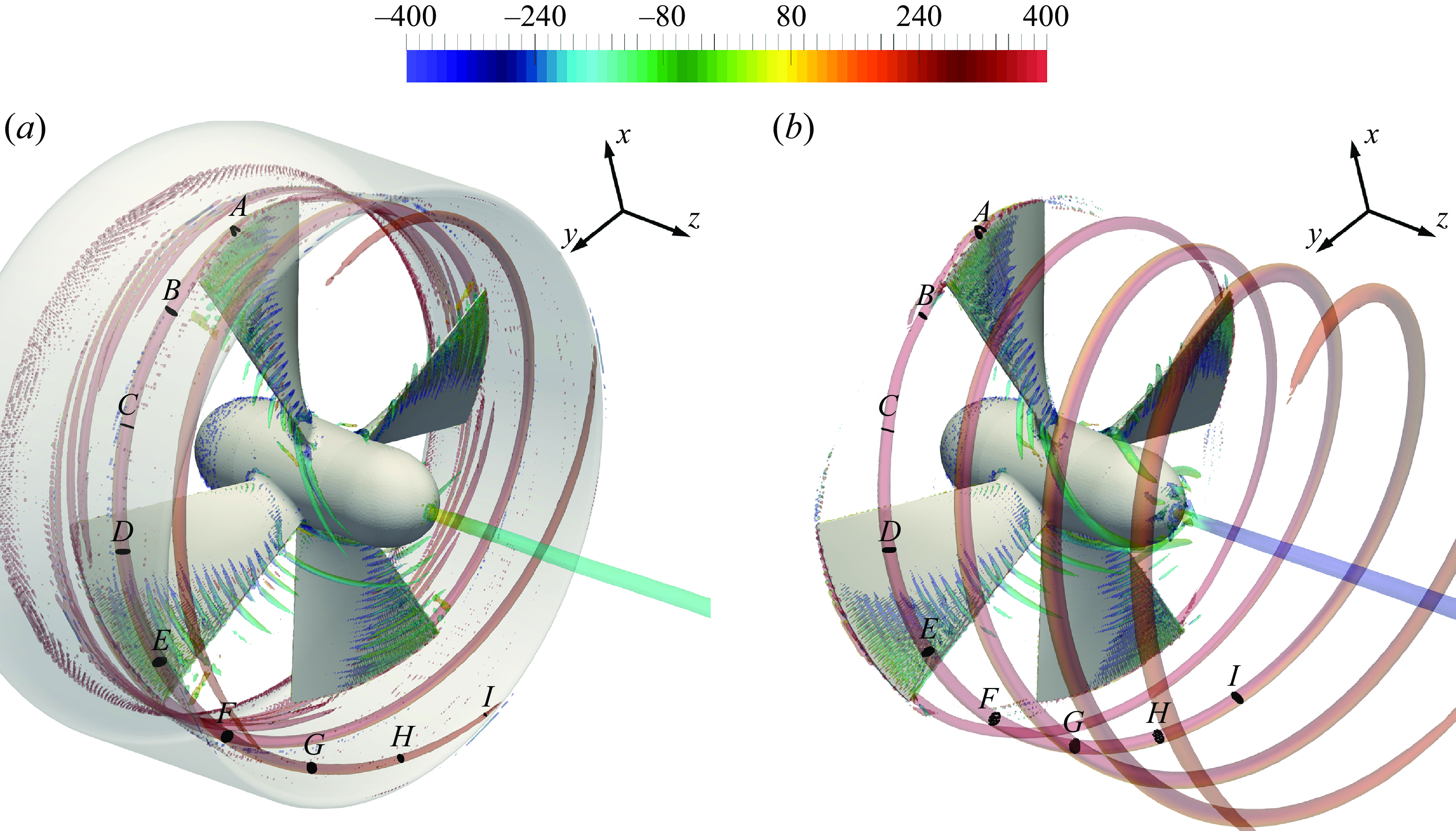
Contours of phase-averaged azimuthal vorticity, scaled by $U_\infty /D$
, just downstream of the ducted propeller on meridian slices of the computational grid. Isolines for
$U_\infty /D$
, just downstream of the ducted propeller on meridian slices of the computational grid. Isolines for $\widehat {\mathcal {Q}}D^2/U_\infty ^2=10\,000$
. The black isolines encompassing the cross-sections shown in figure 16(a): (a)
$\widehat {\mathcal {Q}}D^2/U_\infty ^2=10\,000$
. The black isolines encompassing the cross-sections shown in figure 16(a): (a) $A$
, (b)
$A$
, (b) $B$
, (c)
$B$
, (c) $C$
, (d)
$C$
, (d) $D$
, (e)
$D$
, (e) $E$
, (f)
$E$
, (f) $F$
, (g)
$F$
, (g) $G$
, (h)
$G$
, (h) $H$
and (i)
$H$
and (i) $I$
.
$I$
.
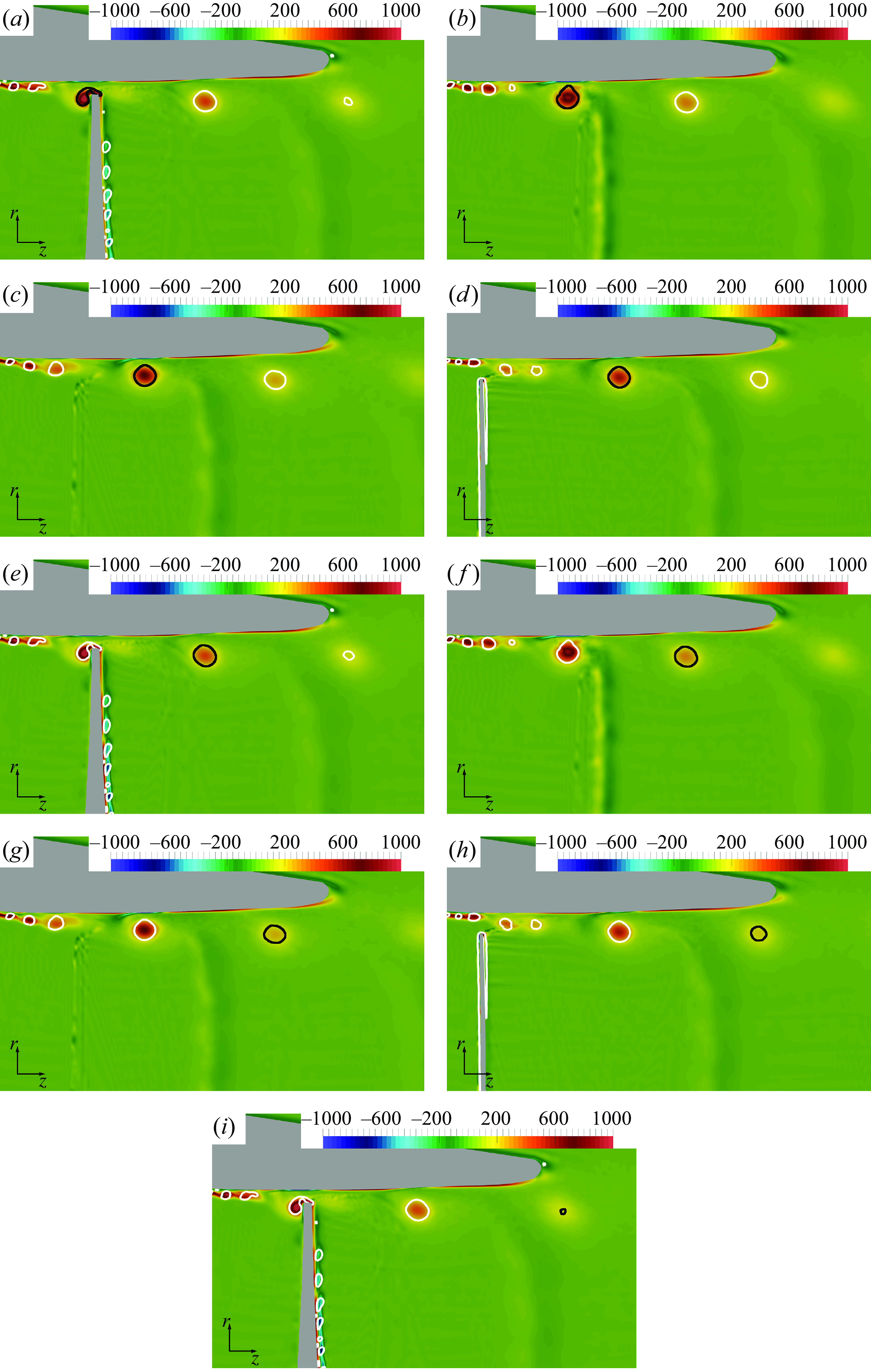
Contours of phase-averaged azimuthal vorticity, scaled by $U_\infty /D$
, just downstream of the conventional propeller on meridian slices of the computational grid. Isolines for
$U_\infty /D$
, just downstream of the conventional propeller on meridian slices of the computational grid. Isolines for $\widehat {\mathcal {Q}}D^2/U_\infty ^2=10\,000$
. The black isolines encompassing the cross-sections shown in figure 16(b): (a)
$\widehat {\mathcal {Q}}D^2/U_\infty ^2=10\,000$
. The black isolines encompassing the cross-sections shown in figure 16(b): (a) $A$
, (b)
$A$
, (b) $B$
, (c)
$B$
, (c) $C$
, (d)
$C$
, (d) $D$
, (e)
$D$
, (e) $E$
, (f)
$E$
, (f) $F$
, (g)
$F$
, (g) $G$
, (h)
$G$
, (h) $H$
and (i)
$H$
and (i) $I$
.
$I$
.
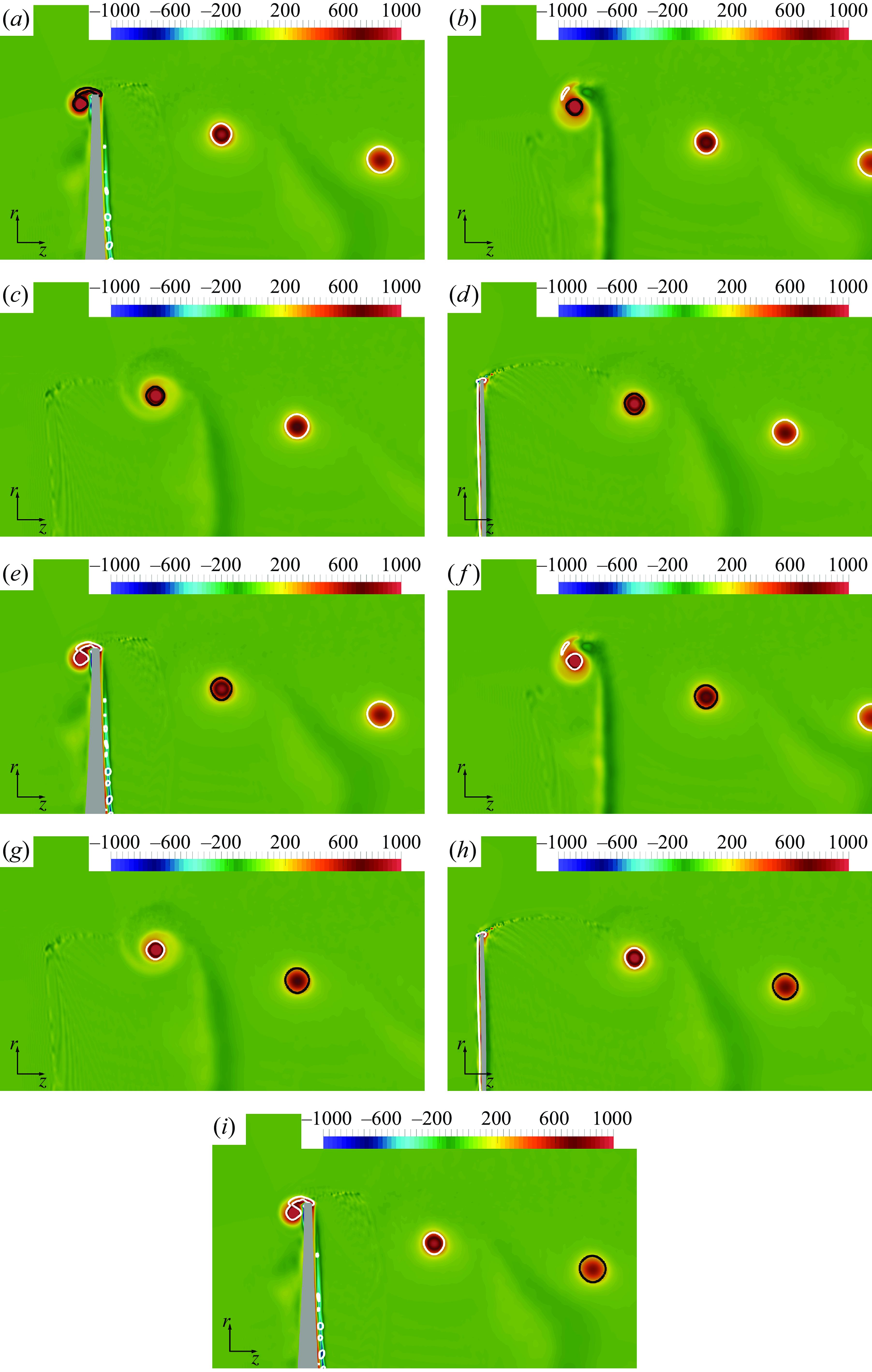
Contours of $\widehat {u'w'}$
, scaled by
$\widehat {u'w'}$
, scaled by $U_\infty ^2$
, just downstream of the ducted propeller on meridian slices of the computational grid. Isolines for
$U_\infty ^2$
, just downstream of the ducted propeller on meridian slices of the computational grid. Isolines for $\widehat {\mathcal {Q}}D^2/U_\infty ^2=10\,000$
. The black isolines encompassing the cross-sections shown in figure 16(a): (a)
$\widehat {\mathcal {Q}}D^2/U_\infty ^2=10\,000$
. The black isolines encompassing the cross-sections shown in figure 16(a): (a) $A$
, (b)
$A$
, (b) $B$
, (c)
$B$
, (c) $C$
, (d)
$C$
, (d) $D$
, (e)
$D$
, (e) $E$
, (f)
$E$
, (f) $F$
, (g)
$F$
, (g) $G$
, (h)
$G$
, (h) $H$
and (i)
$H$
and (i) $I$
.
$I$
.
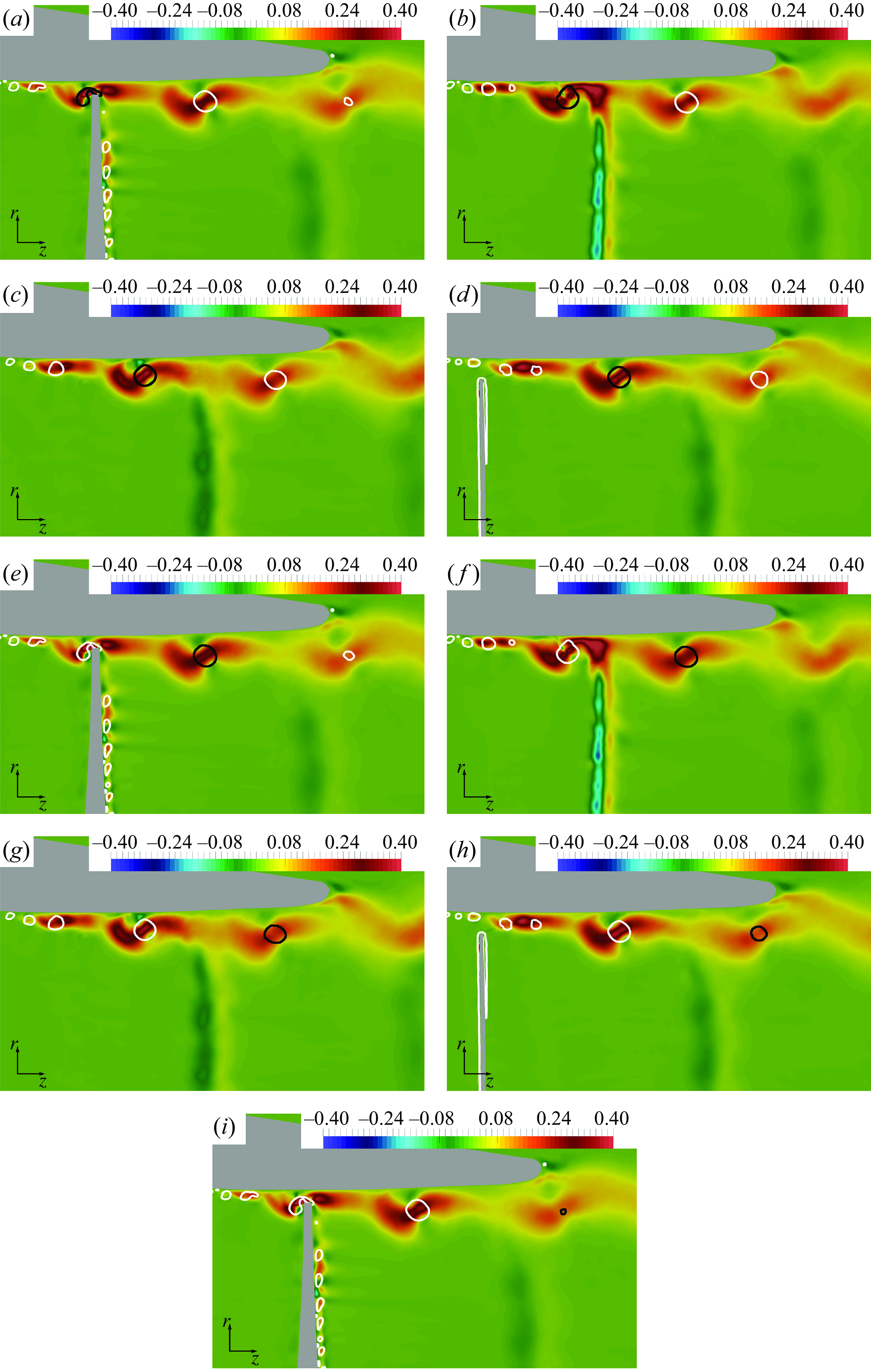
Contours of $\widehat {u'w'}$
, scaled by
$\widehat {u'w'}$
, scaled by $U_\infty ^2$
, just downstream of the conventional propeller on meridian slices of the computational grid. Isolines for
$U_\infty ^2$
, just downstream of the conventional propeller on meridian slices of the computational grid. Isolines for $\widehat {\mathcal {Q}}D^2/U_\infty ^2=10\,000$
. The black isolines encompassing the cross-sections shown in figure 16(b): (a)
$\widehat {\mathcal {Q}}D^2/U_\infty ^2=10\,000$
. The black isolines encompassing the cross-sections shown in figure 16(b): (a) $A$
, (b)
$A$
, (b) $B$
, (c)
$B$
, (c) $C$
, (d)
$C$
, (d) $D$
, (e)
$D$
, (e) $E$
, (f)
$E$
, (f) $F$
, (g)
$F$
, (g) $G$
, (h)
$G$
, (h) $H$
and (i)
$H$
and (i) $I$
.
$I$
.
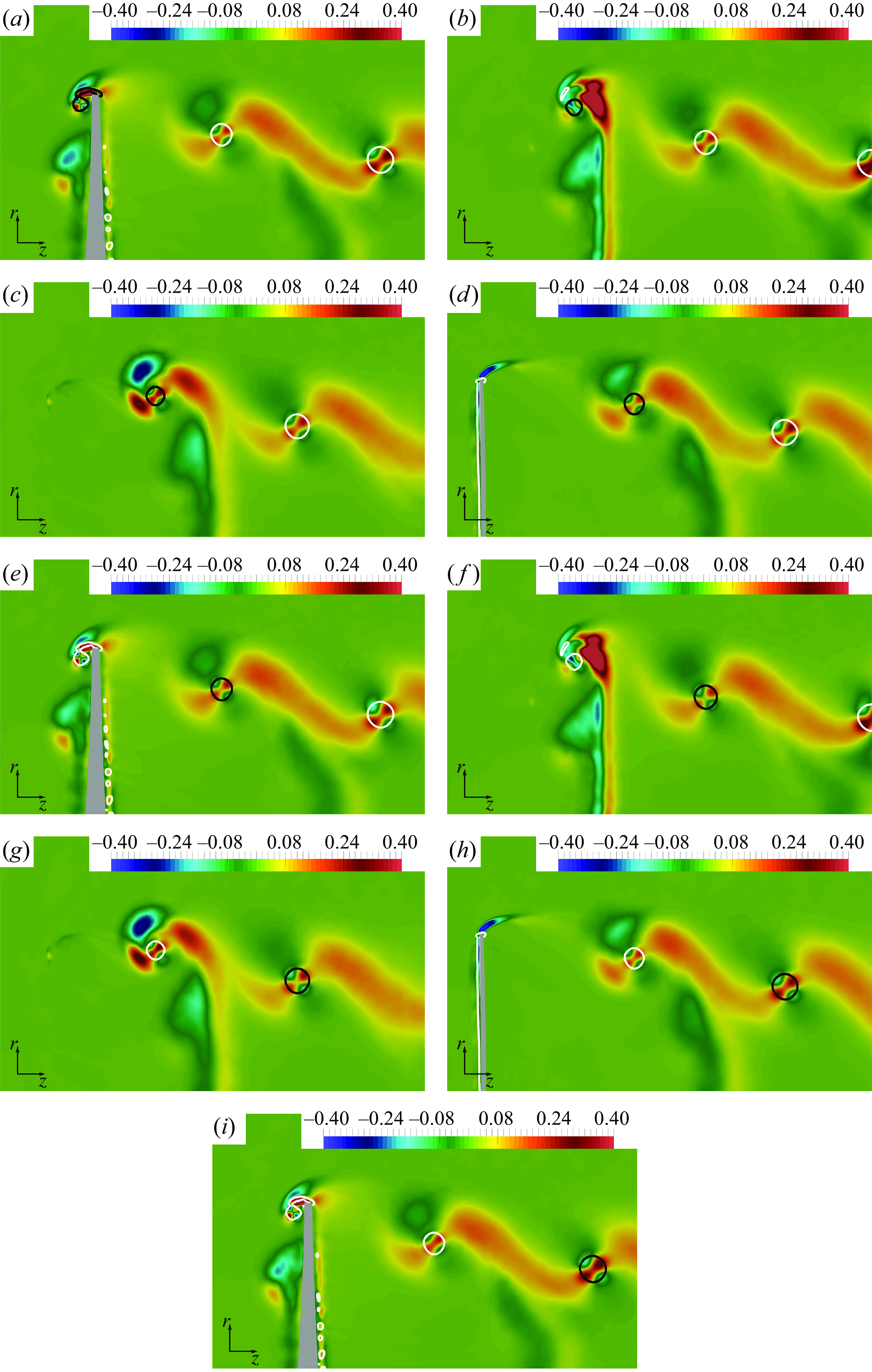
Phase-averaged statistics at the cross-sections of the vortices illustrated in figure 16: (a) circulation, (b) average of the pressure coefficient over the cross sections, (c) radial coordinate of the vortices, (d) streamwise coordinate of the vortices.
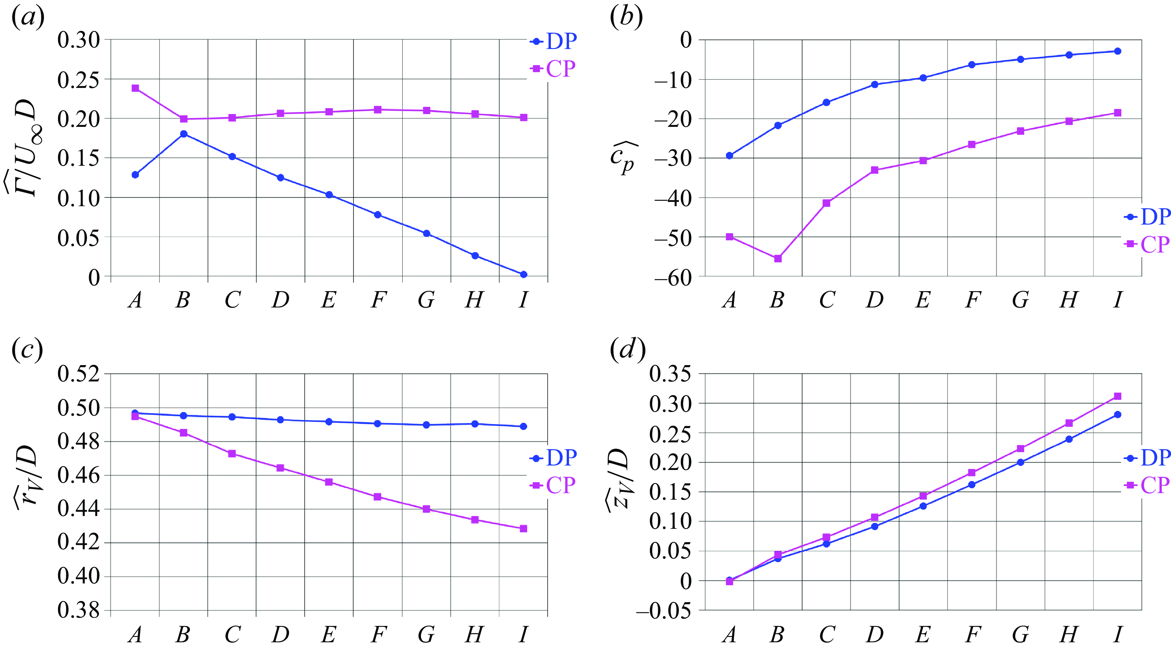
Figures 17 and 18 show results for the phase-averaged fields of azimuthal vorticity on the azimuthal planes of each section of figure 16. The isolines enclose the regions of $\widehat {\mathcal {Q}}D^2/U_\infty ^2 \gt 10\,000$
, adopted to isolate the cores of the tip and tip leakage vortices. In particular, the black isolines encompass the vortices of the cross-sections indicated in figure 16. It is clear that the diffusion of the vorticity peak at the core of the tip leakage vortex in figure 17 is much faster than that affecting the core of the tip vortex in figure 18. This is the result of the shear occurring between the tip leakage vortex and the boundary layer on the inner surface of the duct. This shear is especially reflected in the contours of the turbulent shear stress
$\widehat {\mathcal {Q}}D^2/U_\infty ^2 \gt 10\,000$
, adopted to isolate the cores of the tip and tip leakage vortices. In particular, the black isolines encompass the vortices of the cross-sections indicated in figure 16. It is clear that the diffusion of the vorticity peak at the core of the tip leakage vortex in figure 17 is much faster than that affecting the core of the tip vortex in figure 18. This is the result of the shear occurring between the tip leakage vortex and the boundary layer on the inner surface of the duct. This shear is especially reflected in the contours of the turbulent shear stress $\widehat {u'w'}$
, which is higher at the core of the tip leakage vortices and in their vicinity, if compared with the same quantity for the tip vortices shed by the conventional propeller. This is shown by the comparison between figures 19 and 20. These results are represented more quantitatively in figure 21.
$\widehat {u'w'}$
, which is higher at the core of the tip leakage vortices and in their vicinity, if compared with the same quantity for the tip vortices shed by the conventional propeller. This is shown by the comparison between figures 19 and 20. These results are represented more quantitatively in figure 21.
Figure 21(a) shows the circulation $\widehat {\Gamma }$
at the core of the vortices, computed on the cross-sections shown in figure 16. While
$\widehat {\Gamma }$
at the core of the vortices, computed on the cross-sections shown in figure 16. While $\widehat {\Gamma }$
is rather uniform across sections of the tip vortex shed by the conventional propeller, this is not the case for the tip leakage vortex. Between sections
$\widehat {\Gamma }$
is rather uniform across sections of the tip vortex shed by the conventional propeller, this is not the case for the tip leakage vortex. Between sections $A$
and
$A$
and $B$
the circulation of the tip leakage vortex experiences an increase, since section
$B$
the circulation of the tip leakage vortex experiences an increase, since section $A$
is at about the mid chord of the propeller blade and the vortex is still in formation, while starting from section
$A$
is at about the mid chord of the propeller blade and the vortex is still in formation, while starting from section $B$
its circulation experiences a dramatic decrease. As a result, while at section
$B$
its circulation experiences a dramatic decrease. As a result, while at section $B$
the two vortices still display only small deviations in terms of circulation, they grow dramatically as the tip leakage vortex moves across the nozzle.
$B$
the two vortices still display only small deviations in terms of circulation, they grow dramatically as the tip leakage vortex moves across the nozzle.
Differences are more evident when considering the pressure coefficient at the core of the vortices, represented in figure 21(b). This was averaged within the region identified by the cross-sections of figure 16. These differences are important, taking into account that the minima of pressure achieved within the core of the vortices are potential regions of inception of cavitation phenomena. Figure 21(c,d) also provides information on the trajectory of the vortices, reporting the radial and streamwise coordinates of their cores, respectively. Interestingly, while the tip vortex shed by the conventional propeller experiences the expected shift towards inner radial coordinates, as a result of the acceleration of the flow and the resulting wake contraction, the inward shift of the tip leakage vortices is much smaller: at the section $I$
this shift is equal to about
$I$
this shift is equal to about $0.07D$
for the tip vortex and
$0.07D$
for the tip vortex and $0.01D$
for the tip leakage vortex. This difference may be attributed to two major sources: (i) the thrust produced by the rotor of the ducted propeller is only
$0.01D$
for the tip leakage vortex. This difference may be attributed to two major sources: (i) the thrust produced by the rotor of the ducted propeller is only $61\,\%$
of that produced by the conventional propeller, resulting in a smaller acceleration of the flow in its wake; (ii) the shear with the boundary layer on the inner surface of the nozzle is damping the inward shift of the tip leakage vortex. The impact of this shear on the evolution of the tip leakage vortex is also reflected in figure 21(d), showing that this vortex is advancing in the streamwise direction at a slower rate, in comparison with the tip vortex. This result is not obvious. Typically, higher levels of thrust of conventional propellers result in a more intense cross-flow from the pressure side towards the suction side at the tip of the blades, producing a smaller pitch of the tip vortices, which means a smaller angle relative to the azimuthal direction and a slower advancement in the streamwise direction. We verified that the blades of the ducted propeller are producing a smaller thrust than those of the conventional propeller. Nonetheless, the results in figure 21(d) show that the pitch of the tip leakage vortex of the ducted propeller is smaller than that of the tip vortex of the conventional propeller. This result can be again attributed to the shear developed between the tip leakage vortex and the boundary layer on the inner surface of the duct, generating an additional resistance to the streamwise advancement of the tip leakage vortex and resulting in a smaller pitch, compared with the tip vortex shed by the conventional propeller.
$61\,\%$
of that produced by the conventional propeller, resulting in a smaller acceleration of the flow in its wake; (ii) the shear with the boundary layer on the inner surface of the nozzle is damping the inward shift of the tip leakage vortex. The impact of this shear on the evolution of the tip leakage vortex is also reflected in figure 21(d), showing that this vortex is advancing in the streamwise direction at a slower rate, in comparison with the tip vortex. This result is not obvious. Typically, higher levels of thrust of conventional propellers result in a more intense cross-flow from the pressure side towards the suction side at the tip of the blades, producing a smaller pitch of the tip vortices, which means a smaller angle relative to the azimuthal direction and a slower advancement in the streamwise direction. We verified that the blades of the ducted propeller are producing a smaller thrust than those of the conventional propeller. Nonetheless, the results in figure 21(d) show that the pitch of the tip leakage vortex of the ducted propeller is smaller than that of the tip vortex of the conventional propeller. This result can be again attributed to the shear developed between the tip leakage vortex and the boundary layer on the inner surface of the duct, generating an additional resistance to the streamwise advancement of the tip leakage vortex and resulting in a smaller pitch, compared with the tip vortex shed by the conventional propeller.
Phase-averaged statistics at the cross-sections of the vortices illustrated in figure 16: averages over the cross-sections of (a) $\widehat {k}$
, (b)
$\widehat {k}$
, (b) $|\widehat {u'v'}|$
, (c)
$|\widehat {u'v'}|$
, (c) $|\widehat {u'w'}|$
and (d)
$|\widehat {u'w'}|$
and (d) $|\widehat {v'w'}|$
.
$|\widehat {v'w'}|$
.
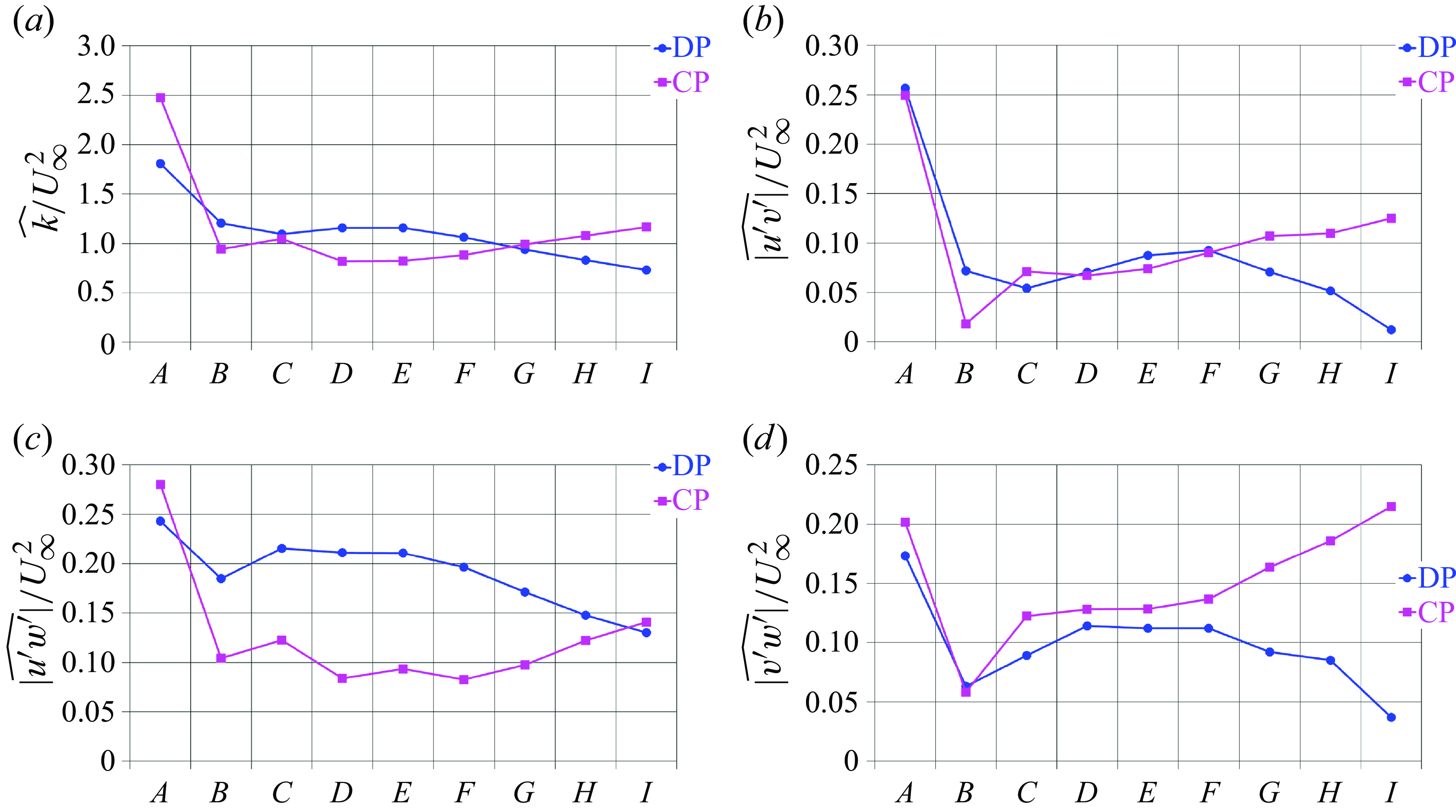
Second-order statistics at the core of the vortices are reported in figure 22. Note that the values for the turbulent shear stresses were computed as averages of their magnitude within the core of the vortices, since in general they can achieve both positive and negative peaks. The most important deviations between the two cases occur in figure 22(c), dealing with the turbulent shear stress $\widehat {u'w'}$
. There, the turbulent stresses achieved within the core of the tip leakage vortex are approximately double those at the core of the tip vortex, despite the weaker intensity of the former, compared with the latter. In addition, figures 19 and 20 demonstrate that these large deviations between the two propellers extend even outside the core of the vortices, as a result of the shear developed between the tip leakage vortex and the boundary layer of the nozzle, which is obviously missing in the case of the conventional propeller. In our earlier studies we found that the increase of this shear stress correlates with the onset of the instability of the tip vortices of conventional propellers (Posa et al. Reference Posa, Broglia and Balaras2019a
, Reference Posa, Broglia and Balaras2022a
, Posa Reference Posa2022a
). For conventional propellers, this is the result of the shear developing between the tip vortices and the trailing wake of the following blades, since the tip vortices are characterised by a smaller pitch compared with the trailing wake, which means a slower streamwise advancement downstream of the propeller plane. Therefore, downstream of the propeller plane the tip vortices experience shear with the trailing wake of the following blades, which moves downstream at a faster rate. This is also the case of the conventional propeller considered in this study. In contrast, the rise of the shear stress
$\widehat {u'w'}$
. There, the turbulent stresses achieved within the core of the tip leakage vortex are approximately double those at the core of the tip vortex, despite the weaker intensity of the former, compared with the latter. In addition, figures 19 and 20 demonstrate that these large deviations between the two propellers extend even outside the core of the vortices, as a result of the shear developed between the tip leakage vortex and the boundary layer of the nozzle, which is obviously missing in the case of the conventional propeller. In our earlier studies we found that the increase of this shear stress correlates with the onset of the instability of the tip vortices of conventional propellers (Posa et al. Reference Posa, Broglia and Balaras2019a
, Reference Posa, Broglia and Balaras2022a
, Posa Reference Posa2022a
). For conventional propellers, this is the result of the shear developing between the tip vortices and the trailing wake of the following blades, since the tip vortices are characterised by a smaller pitch compared with the trailing wake, which means a slower streamwise advancement downstream of the propeller plane. Therefore, downstream of the propeller plane the tip vortices experience shear with the trailing wake of the following blades, which moves downstream at a faster rate. This is also the case of the conventional propeller considered in this study. In contrast, the rise of the shear stress $\widehat {u'w'}$
occurs earlier at the core of the tip leakage vortices, since their instability comes from a different source, which is the shear with the boundary layer of the nozzle. This faster instability explains the faster decay of vorticity and circulation at the core of the tip leakage vortices and is also in line with the turbulent stresses reported in figure 22. Turbulent kinetic energy as well as the turbulent shear stresses
$\widehat {u'w'}$
occurs earlier at the core of the tip leakage vortices, since their instability comes from a different source, which is the shear with the boundary layer of the nozzle. This faster instability explains the faster decay of vorticity and circulation at the core of the tip leakage vortices and is also in line with the turbulent stresses reported in figure 22. Turbulent kinetic energy as well as the turbulent shear stresses $\widehat {u'v'}$
and
$\widehat {u'v'}$
and $\widehat {v'w'}$
are initially similar at the core of the tip and tip leakage vortices. However, as the tip leakage vortex experiences instability and diffusion, gradients and turbulence at its core in the phase-averaged statistics decline. This is even the case of the shear stress
$\widehat {v'w'}$
are initially similar at the core of the tip and tip leakage vortices. However, as the tip leakage vortex experiences instability and diffusion, gradients and turbulence at its core in the phase-averaged statistics decline. This is even the case of the shear stress $\widehat {u'w'}$
, which at the last cross-section
$\widehat {u'w'}$
, which at the last cross-section $I$
is already similar between the cores of the tip and tip leakage vortices, due to the diffusion of the tip leakage vortex.
$I$
is already similar between the cores of the tip and tip leakage vortices, due to the diffusion of the tip leakage vortex.
Contours of time-averaged streamwise velocity on a meridian plane, scaled by $U_\infty$
: (a) ducted and (b) conventional propellers.
$U_\infty$
: (a) ducted and (b) conventional propellers.

Radial profiles of time-averaged streamwise velocity at the streamwise coordinate $z/D=0.2$
: (a) comparison between ducted and conventional propellers on the fine grid and (b) comparison across grid resolutions for the ducted propeller.
$z/D=0.2$
: (a) comparison between ducted and conventional propellers on the fine grid and (b) comparison across grid resolutions for the ducted propeller.
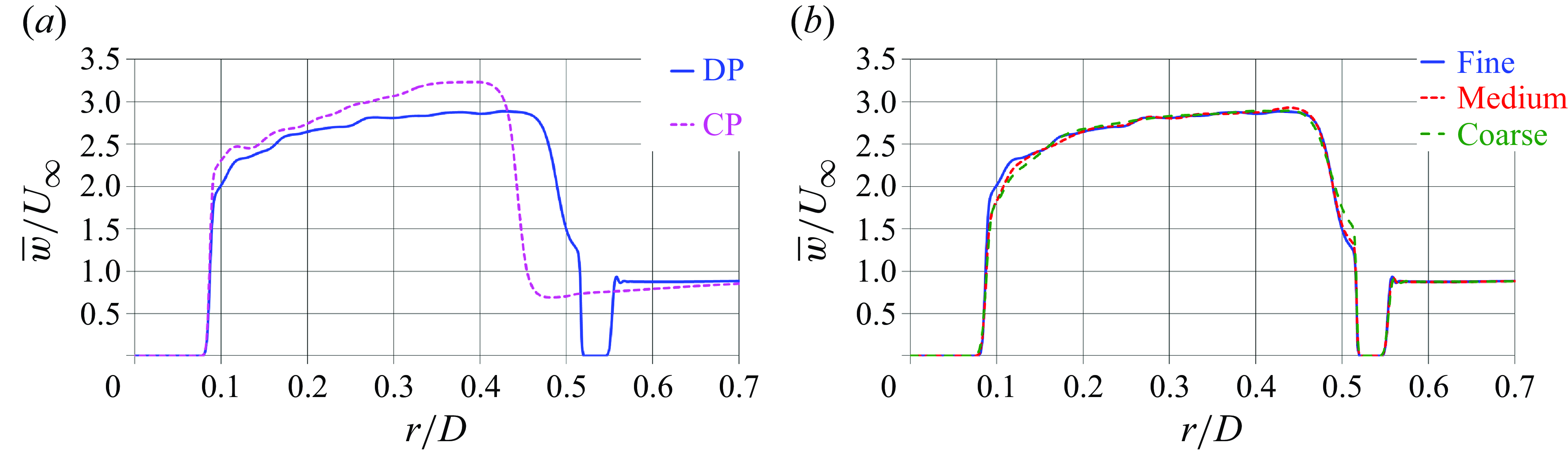
Contours of time-averaged turbulent kinetic energy on a meridian plane, scaled by $U_\infty ^2$
: (a) ducted and (b) conventional propellers.
$U_\infty ^2$
: (a) ducted and (b) conventional propellers.
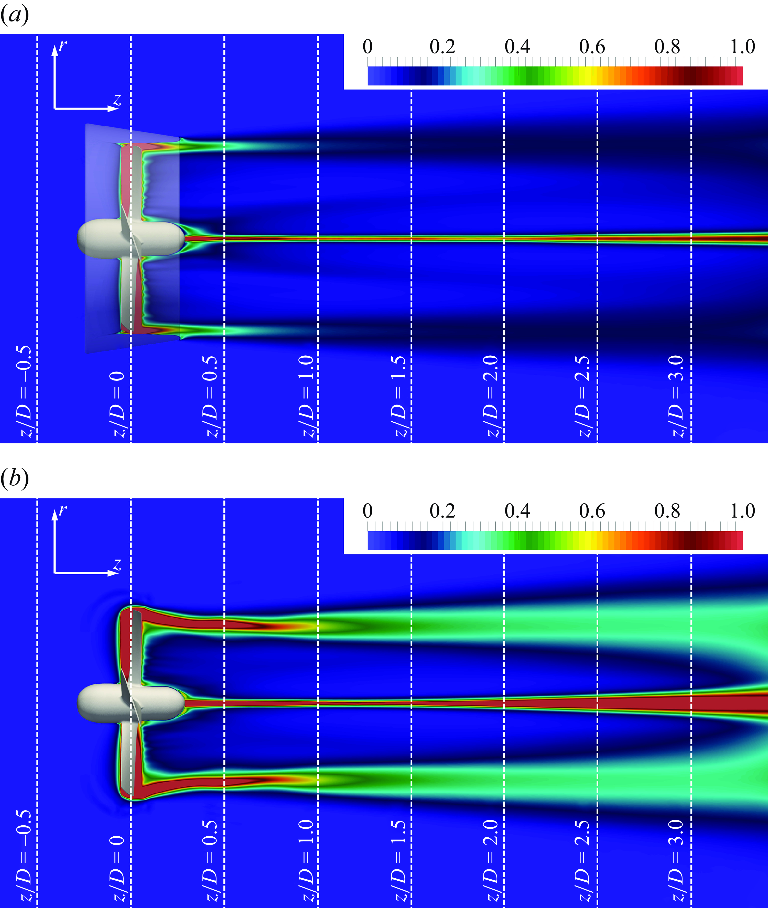
Radial profiles of time-averaged turbulent kinetic energy at the streamwise coordinate $z/D=0.2$
: (a) comparison between ducted and conventional propellers on the fine grid and (b) comparison across grid resolutions for the ducted propeller.
$z/D=0.2$
: (a) comparison between ducted and conventional propellers on the fine grid and (b) comparison across grid resolutions for the ducted propeller.
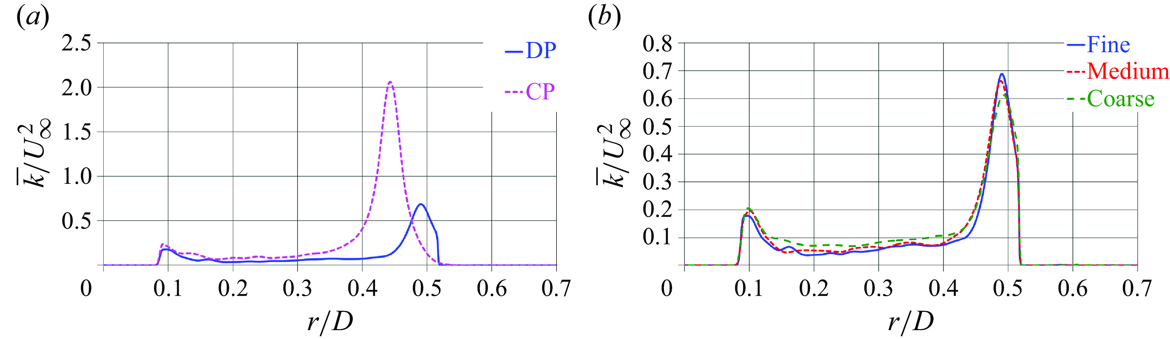
Contours of time-averaged turbulent shear stresses downstream of the ducted propeller on a meridian plane, scaled by $U_\infty ^2$
: (a)
$U_\infty ^2$
: (a) $\overline {u'v'}$
(b)
$\overline {u'v'}$
(b) $\overline {u'w'}$
and (c)
$\overline {u'w'}$
and (c) $\overline {v'w'}$
.
$\overline {v'w'}$
.
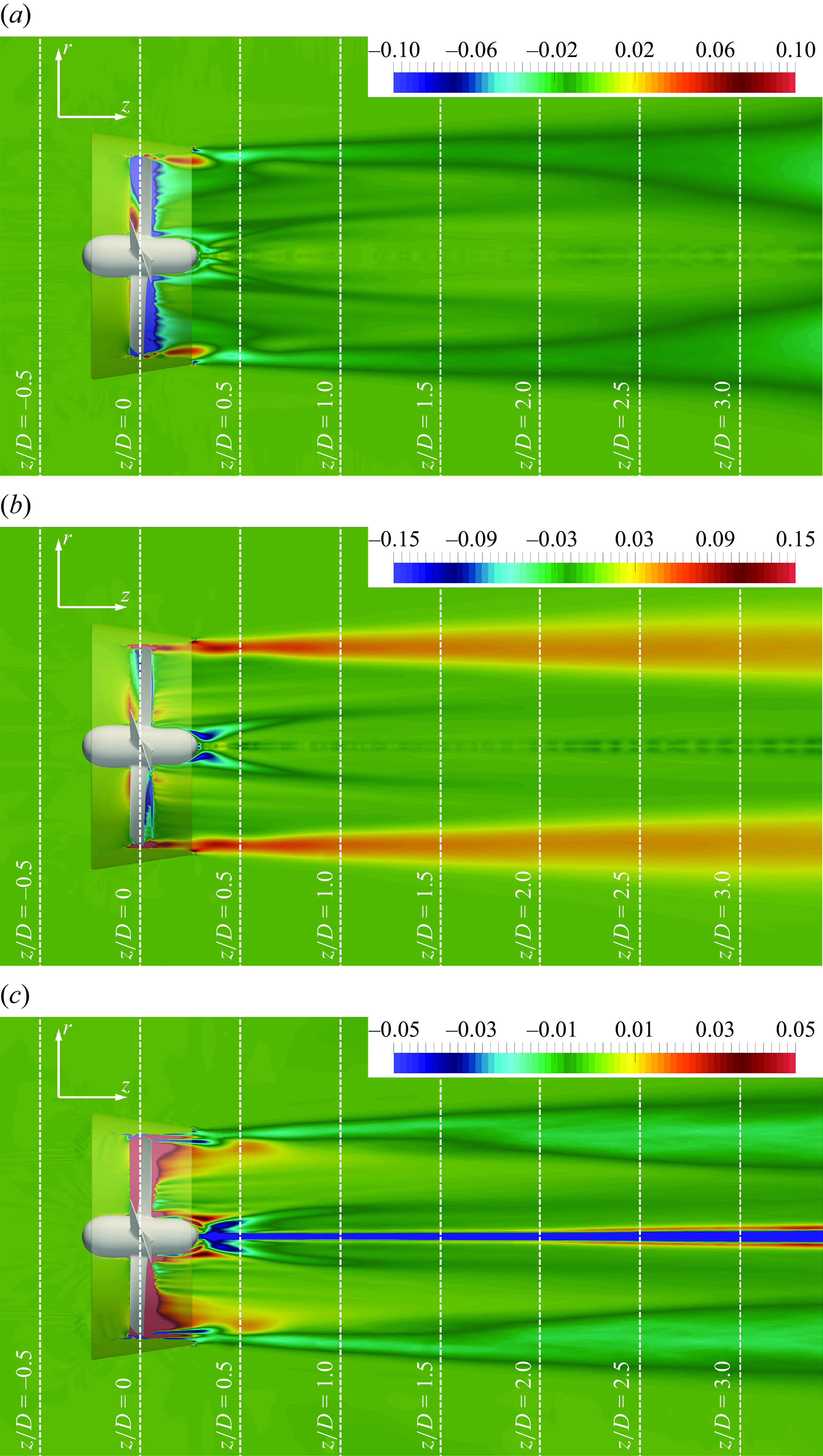
Contours of time-averaged turbulent shear stresses downstream of the conventional propeller on a meridian plane, scaled by $U_\infty ^2$
: (a)
$U_\infty ^2$
: (a) $\overline {u'v'}$
(b)
$\overline {u'v'}$
(b) $\overline {u'w'}$
and (c)
$\overline {u'w'}$
and (c) $\overline {v'w'}$
.
$\overline {v'w'}$
.
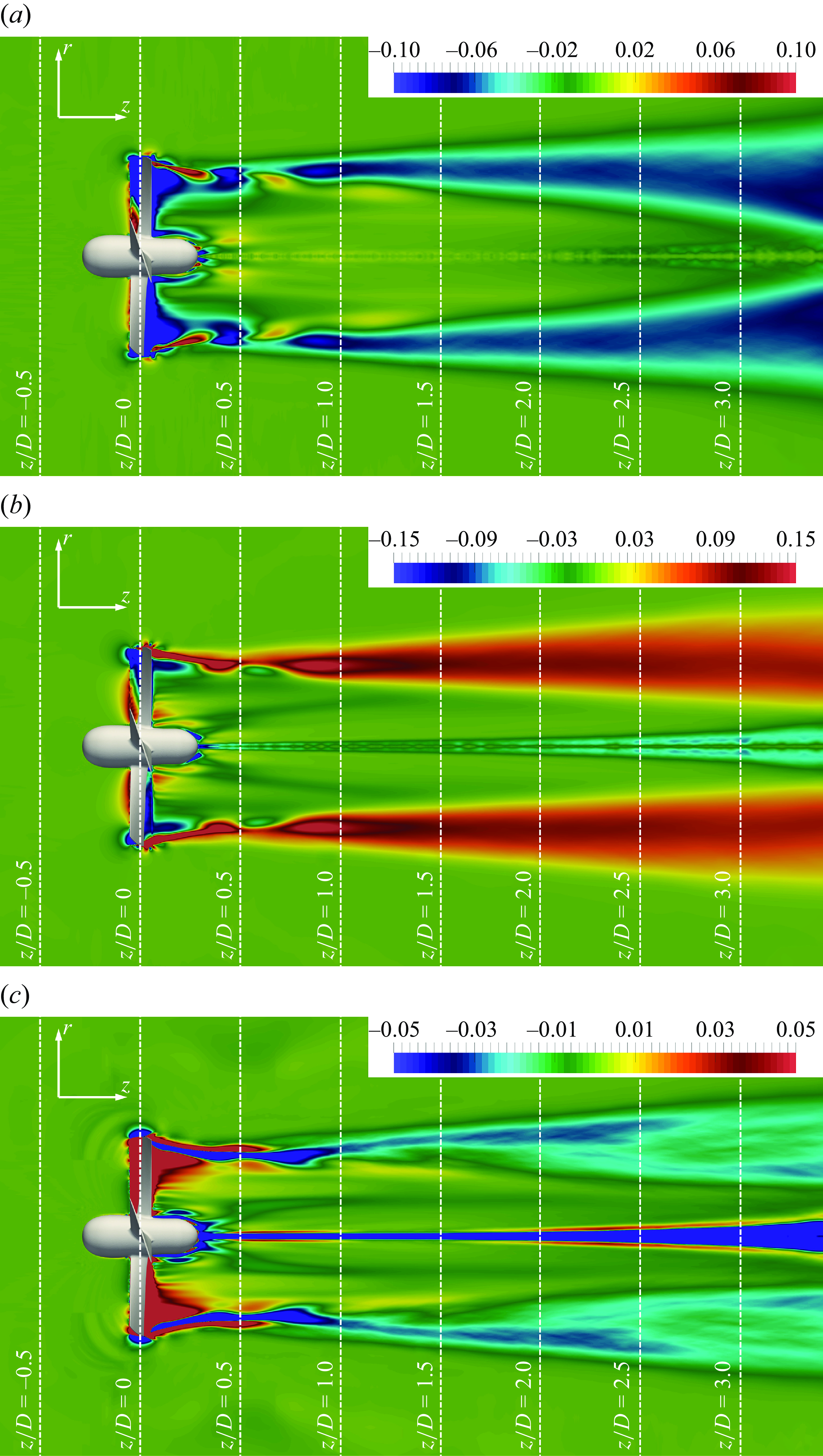
5.5. Time-averaged statistics in the wake
Contours of time-averaged streamwise velocity on a meridian plane are shown in figure 23. It is interesting to see that the flow downstream of the ducted propeller displays a weaker acceleration, compared with the case of the conventional propeller, as illustrated in more detail by the radial profiles in figure 24(a), dealing with the streamwise location at $z/D=0.2$
. This result is consistent with the global performance discussed in § 5.1: the thrust produced by the ducted propeller is smaller than that generated by the conventional propeller. As a result, the wake of the ducted propeller experiences a smaller contraction, in comparison with that of the conventional propeller. Although this result may appear counterintuitive, taking into account the acceleration of the incoming flow promoted by the presence of the nozzle, it is actually in line with the changes of the inflow conditions of the rotor of the ducted propeller. As discussed above, the typical characteristic curves of marine propellers show that increasing values of inflow velocity, corresponding to higher values of advance coefficient and a modification of the incidence angle of the flow ingested by the propeller blades, result in a lower thrust. In other words, although the advance velocity and the rotational speed of the ducted propeller are the same as those of the conventional propeller, the nozzle of the former is changing the actual working conditions of its blades, which move towards a higher value of the advance coefficient, equivalent to lower loads and a lower thrust, compensated in part by the additional thrust produced by the nozzle itself, as we verified above in § 5.1 through the analysis of global performance. Therefore, the acceleration experienced by the flow across the ducted propeller is actually smaller, due to the lower thrust it generates. As a consequence, the conservation of mass implies a smaller contraction of the streamtube through the propeller, due to the lower values of streamwise velocity gained by the flow through the ducted propeller, in comparison with the conventional one. This is the same reason why all studies exploring the wake development of propellers across a range of working conditions find decreasing wake contractions for increasing advance coefficients, equivalent to decreasing levels of thrust and acceleration of the flow (Muscari et al. Reference Muscari, Di Mascio and Verzicco2013; Baek et al. Reference Baek, Yoon, Jung, Kim and Paik2015; Wang et al. Reference Wang, Li, Han and Hao2022a
; Posa & Broglia Reference Posa and Broglia2023). This result is also illustrated in the radial profiles of figure 24, where lower values of streamwise velocity downstream of the ducted propeller, in comparison with the conventional propeller, imply a wider radial extent of its wake. The results in figure 24(a), showing that the deviations between the two wake flows extend to inner radial coordinates, are also in line with the visualisations in figures 13 and 14, where the topology of the wake structures is modified across the whole spanwise extent of the propeller. In figure 24(b) comparisons across grid resolutions are also reported, demonstrating a very limited grid dependence of the solution.
$z/D=0.2$
. This result is consistent with the global performance discussed in § 5.1: the thrust produced by the ducted propeller is smaller than that generated by the conventional propeller. As a result, the wake of the ducted propeller experiences a smaller contraction, in comparison with that of the conventional propeller. Although this result may appear counterintuitive, taking into account the acceleration of the incoming flow promoted by the presence of the nozzle, it is actually in line with the changes of the inflow conditions of the rotor of the ducted propeller. As discussed above, the typical characteristic curves of marine propellers show that increasing values of inflow velocity, corresponding to higher values of advance coefficient and a modification of the incidence angle of the flow ingested by the propeller blades, result in a lower thrust. In other words, although the advance velocity and the rotational speed of the ducted propeller are the same as those of the conventional propeller, the nozzle of the former is changing the actual working conditions of its blades, which move towards a higher value of the advance coefficient, equivalent to lower loads and a lower thrust, compensated in part by the additional thrust produced by the nozzle itself, as we verified above in § 5.1 through the analysis of global performance. Therefore, the acceleration experienced by the flow across the ducted propeller is actually smaller, due to the lower thrust it generates. As a consequence, the conservation of mass implies a smaller contraction of the streamtube through the propeller, due to the lower values of streamwise velocity gained by the flow through the ducted propeller, in comparison with the conventional one. This is the same reason why all studies exploring the wake development of propellers across a range of working conditions find decreasing wake contractions for increasing advance coefficients, equivalent to decreasing levels of thrust and acceleration of the flow (Muscari et al. Reference Muscari, Di Mascio and Verzicco2013; Baek et al. Reference Baek, Yoon, Jung, Kim and Paik2015; Wang et al. Reference Wang, Li, Han and Hao2022a
; Posa & Broglia Reference Posa and Broglia2023). This result is also illustrated in the radial profiles of figure 24, where lower values of streamwise velocity downstream of the ducted propeller, in comparison with the conventional propeller, imply a wider radial extent of its wake. The results in figure 24(a), showing that the deviations between the two wake flows extend to inner radial coordinates, are also in line with the visualisations in figures 13 and 14, where the topology of the wake structures is modified across the whole spanwise extent of the propeller. In figure 24(b) comparisons across grid resolutions are also reported, demonstrating a very limited grid dependence of the solution.
A similar representation of the results is provided in figure 25 for the time-averaged turbulent kinetic energy. For the second-order statistics, the differences between the two cases are even more obvious than in figure 23. The wake of the conventional propeller experiences much higher levels of turbulence, especially in the region of the tip and hub vortices. The discussion on the early evolution of the tip and tip leakage vortices in § 5.4 demonstrated that this result in the wake is due to two major sources. (i) The tip vortices shed by the more-loaded conventional propeller are more intense than the tip leakage vortices shed by the ducted propeller. This is also the case of the hub vortex. (ii) The tip leakage vortices experience early instability, due to their shear with the inner surface of the nozzle, leading to a faster diffusion of their signature in the time-averaged fields. Also in this case this comparison is illustrated in more detail in figure 26(a), where radial profiles are shown at the streamwise coordinate $z/D=0.2$
. In these profiles, the peaks of turbulent kinetic energy also highlight that the core of the tip vortices shed by the conventional propeller is located at inner radial coordinates than that of the tip leakage vortices of the ducted propeller, which is evidence of the stronger wake contraction in the former case. In figure 26(b) the comparison across grid resolutions for the ducted propeller provides additional evidence of grid convergence.
$z/D=0.2$
. In these profiles, the peaks of turbulent kinetic energy also highlight that the core of the tip vortices shed by the conventional propeller is located at inner radial coordinates than that of the tip leakage vortices of the ducted propeller, which is evidence of the stronger wake contraction in the former case. In figure 26(b) the comparison across grid resolutions for the ducted propeller provides additional evidence of grid convergence.
Radial profiles of time-averaged turbulent shear stresses (a,b) $\overline {u'v'}$
, (c,d)
$\overline {u'v'}$
, (c,d) $\overline {u'w'}$
and (e,f)
$\overline {u'w'}$
and (e,f) $\overline {v'w'}$
at the streamwise coordinate
$\overline {v'w'}$
at the streamwise coordinate $z/D=0.2$
: (a,c,e) comparison between ducted and conventional propellers on the fine grid and (b,d,f) comparison across grid resolutions for the ducted propeller.
$z/D=0.2$
: (a,c,e) comparison between ducted and conventional propellers on the fine grid and (b,d,f) comparison across grid resolutions for the ducted propeller.
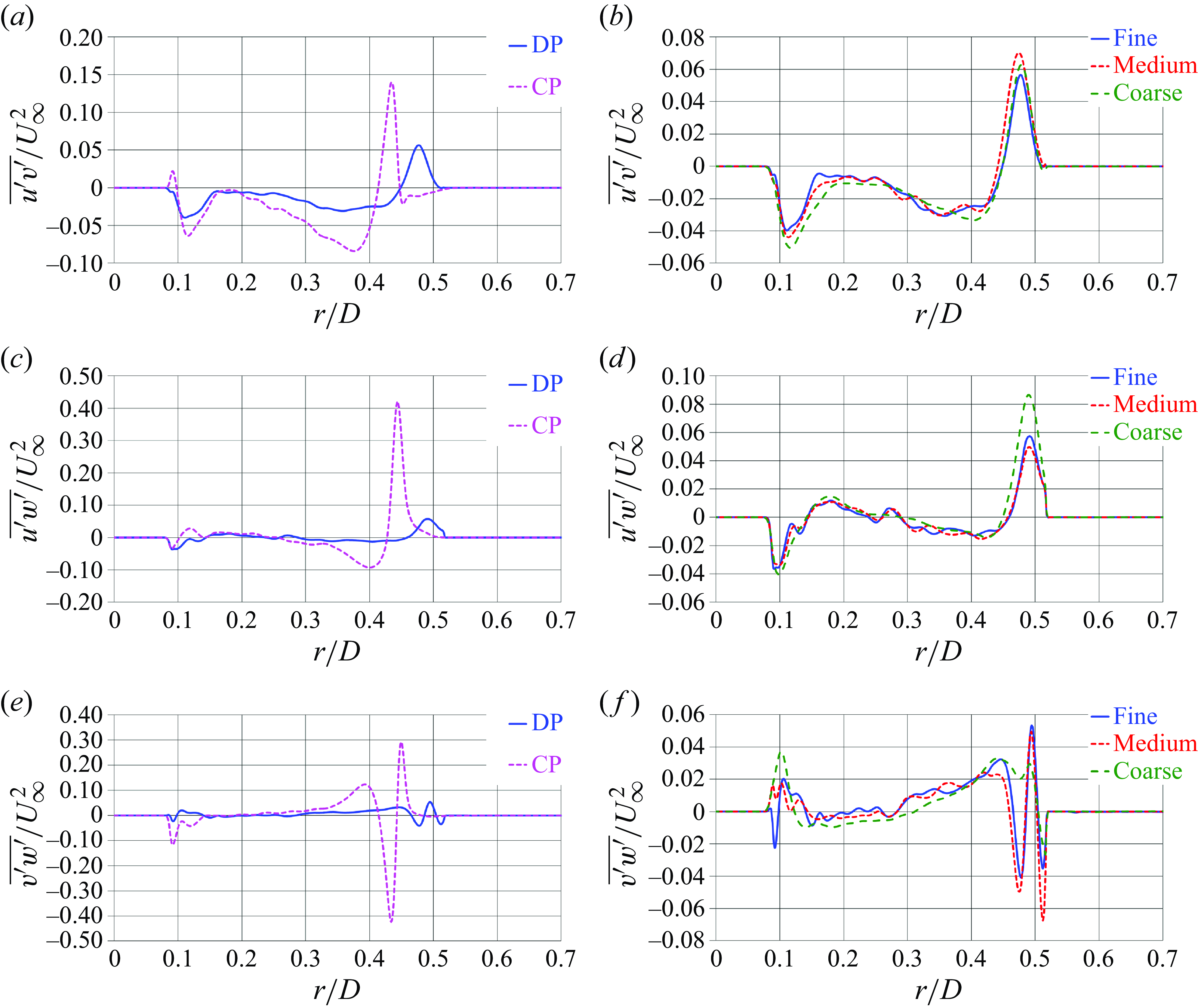
Contours of time-averaged SGS shear stresses downstream of the ducted propeller on a meridian plane, scaled by $U_\infty ^2$
: (a)
$U_\infty ^2$
: (a) $\overline {\tau }_{r \vartheta }$
(b)
$\overline {\tau }_{r \vartheta }$
(b) $\overline {\tau }_{r z}$
and (c)
$\overline {\tau }_{r z}$
and (c) $\overline {\tau }_{\vartheta z}$
.
$\overline {\tau }_{\vartheta z}$
.
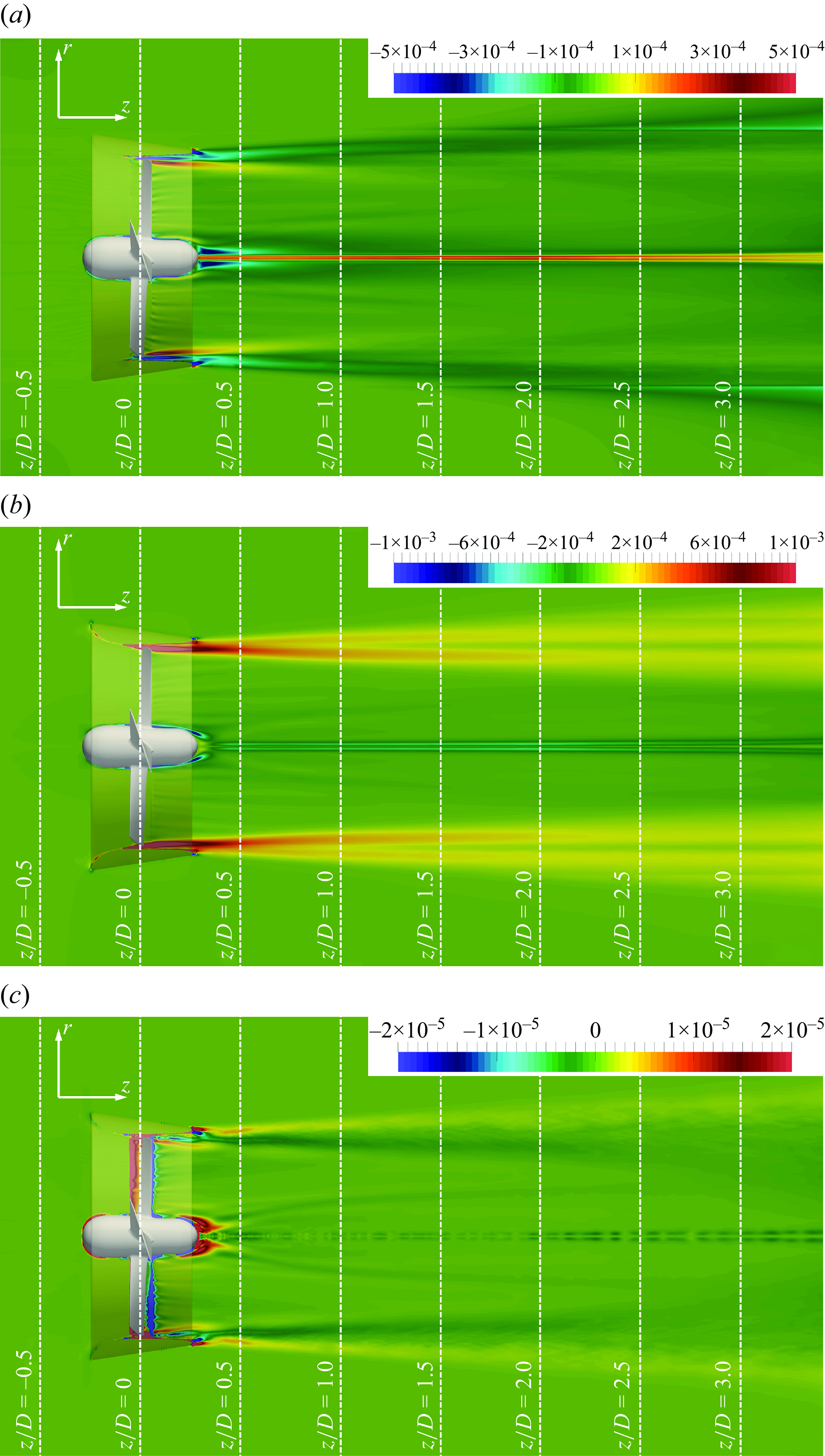
Contours of time-averaged SGS shear stresses downstream of the conventional propeller on a meridian plane, scaled by $U_\infty ^2$
: (a)
$U_\infty ^2$
: (a) $\overline {\tau }_{r \vartheta }$
(b)
$\overline {\tau }_{r \vartheta }$
(b) $\overline {\tau }_{r z}$
and (c)
$\overline {\tau }_{r z}$
and (c) $\overline {\tau }_{\vartheta z}$
.
$\overline {\tau }_{\vartheta z}$
.

All time-averaged turbulent shear stresses in the cylindrical reference frame are shown for the ducted and conventional propellers in figures 27 and 28, respectively. Higher levels of time-averaged turbulence are achieved in the latter case, especially in the region at the outer boundary of the wake, populated by the tip vortices of the conventional propeller and the tip leakage vortices of the ducted propeller. More detailed comparisons are given in figure 29, where the left panels deal with the radial profiles in the wakes of the ducted and conventional propellers at $z/D=0.2$
, while the right panels with the comparison across resolutions for the ducted propeller. These results demonstrate that, for the turbulent stresses
$z/D=0.2$
, while the right panels with the comparison across resolutions for the ducted propeller. These results demonstrate that, for the turbulent stresses $\overline {u'v'}$
and
$\overline {u'v'}$
and $\overline {u'w'}$
, the agreement between the medium and fine grids is close, even for the maxima located at inner and outer radial coordinates, tied to the root and tip leakage vortices, respectively. Deviations are actually more significant for the shear stress
$\overline {u'w'}$
, the agreement between the medium and fine grids is close, even for the maxima located at inner and outer radial coordinates, tied to the root and tip leakage vortices, respectively. Deviations are actually more significant for the shear stress $\overline {v'w'}$
. However, for all stresses, grid dependence is an order of magnitude smaller than the differences between ducted and conventional propellers reported in the left panels of figure 29, confirming that for the latter turbulence in the near wake is almost an order of magnitude higher than for the former.
$\overline {v'w'}$
. However, for all stresses, grid dependence is an order of magnitude smaller than the differences between ducted and conventional propellers reported in the left panels of figure 29, confirming that for the latter turbulence in the near wake is almost an order of magnitude higher than for the former.
The visualisations in figures 30 and 31 show contours of time-averaged modelled shear stresses, to be compared with figures 27 and 28, respectively, dealing with the resolved stresses. In line with the behaviour of the resolved stresses, the modelled stresses are higher in the wake of the conventional propeller, although the ratio with the resolved stresses is similar between the two cases. It is interesting to see that the SGS stresses are at least two orders of magnitude smaller than the resolved stresses. The stress $\overline {\tau }_{\vartheta z}$
is especially small, if compared with
$\overline {\tau }_{\vartheta z}$
is especially small, if compared with $\overline {v'w'}$
: the former is even more than three orders of magnitude smaller than the latter. This result is useful to demonstrate that, thanks to the fine resolution of the computational grid even far away from the bodies immersed within the flow, most turbulence is explicitly resolved, rather than modelled, even when grid coarsening occurs downstream of the propellers. This makes practically negligible the influence on the statistics of turbulence of the particular SGS model adopted for the computations.
$\overline {v'w'}$
: the former is even more than three orders of magnitude smaller than the latter. This result is useful to demonstrate that, thanks to the fine resolution of the computational grid even far away from the bodies immersed within the flow, most turbulence is explicitly resolved, rather than modelled, even when grid coarsening occurs downstream of the propellers. This makes practically negligible the influence on the statistics of turbulence of the particular SGS model adopted for the computations.
As discussed above, the higher levels of turbulent stresses seen in the wake of the conventional propeller are mainly associated with more intense and more stable tip vortices. More intense tip vortices mean a stronger perturbation generated to the downstream flow in a time-averaged sense, resulting in larger fluctuations in time. The following discussion in this section will focus on the streamwise evolution of the time-averaged statistics at the core of the tip and tip leakage vortices. The core of the tip vortices was identified as the peak of turbulent kinetic energy at the outer boundary of the wake. After testing, this criterion was verified the most suitable to track the tip vortices from the propeller plane up to the most downstream coordinates of the computational domain.
Streamwise evolution of the time-averaged (a) vorticity magnitude and (b) pressure coefficient across the trajectory of the tip and tip leakage vortices: comparison between ducted and conventional propellers on the fine grid. The error bars indicate the grid uncertainty with a confidence level of $95\,\%$
from the computations across grid resolutions for the ducted propeller. Note that the horizontal scale is logarithmic.
$95\,\%$
from the computations across grid resolutions for the ducted propeller. Note that the horizontal scale is logarithmic.
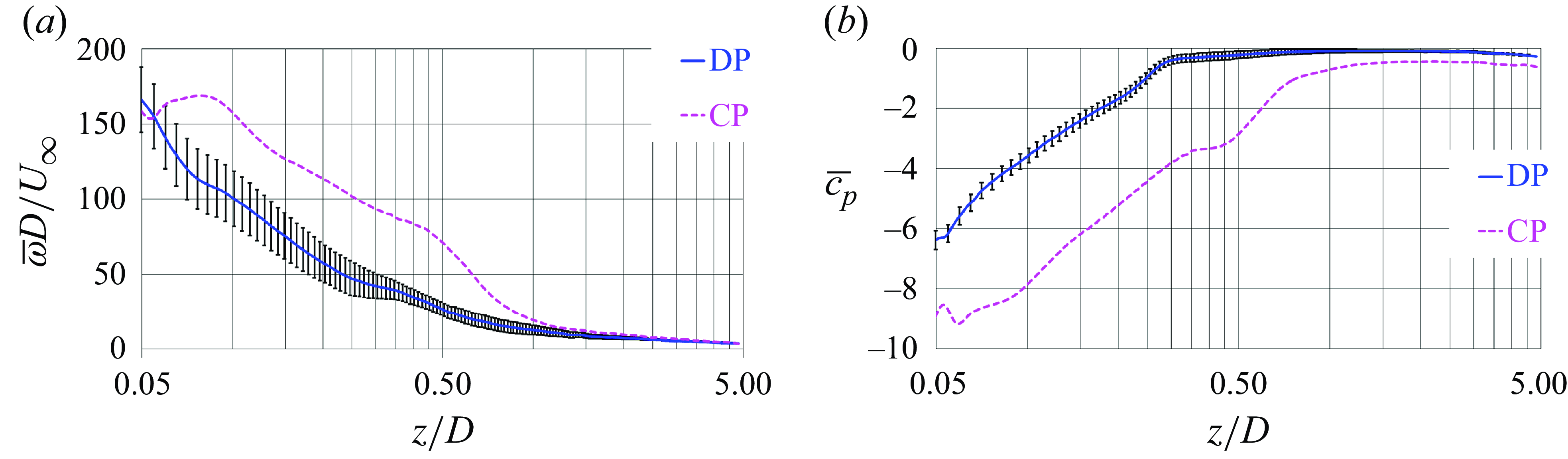
The streamwise evolution of the maxima of the vorticity magnitude and the minima of the pressure coefficient is reported in figure 32, in the left and right panels, respectively. For the case of the ducted propeller, the grid uncertainty with a confidence level of $95\,\%$
was computed from the results on the fine, medium and coarse grids. As discussed in § 5.1, for limitation of computational resources, the simulation on the conventional propeller was carried out on the fine grid only. Meanwhile, the same (fine) computational grid was utilised for both ducted and conventional propellers. Therefore, we do not expect higher levels of uncertainty in the latter case, also taking into account that the physics to be reproduced is actually more challenging in the former case, due to the small gap between the tip of the blades and nozzle. The horizontal scale of the streamwise coordinates is logarithmic, to focus on the region just downstream of the propeller plane, where the streamwise gradients of the statistics are the largest. The maxima of vorticity and minima of pressure associated with the core of the tip vortices from the conventional propeller are substantially higher than those at the core of the tip leakage vortices of the ducted propeller. This is consistent with the discussion above in § 5.4, providing evidence of the stronger intensity and slower diffusion of the former, compared with the latter. The streamwise decay of the maxima in figure 32 is attributable to the increasing instability of the vortices, resulting in the diffusion of the time-averaged statistics. This is faster in the wake of the ducted propeller.
$95\,\%$
was computed from the results on the fine, medium and coarse grids. As discussed in § 5.1, for limitation of computational resources, the simulation on the conventional propeller was carried out on the fine grid only. Meanwhile, the same (fine) computational grid was utilised for both ducted and conventional propellers. Therefore, we do not expect higher levels of uncertainty in the latter case, also taking into account that the physics to be reproduced is actually more challenging in the former case, due to the small gap between the tip of the blades and nozzle. The horizontal scale of the streamwise coordinates is logarithmic, to focus on the region just downstream of the propeller plane, where the streamwise gradients of the statistics are the largest. The maxima of vorticity and minima of pressure associated with the core of the tip vortices from the conventional propeller are substantially higher than those at the core of the tip leakage vortices of the ducted propeller. This is consistent with the discussion above in § 5.4, providing evidence of the stronger intensity and slower diffusion of the former, compared with the latter. The streamwise decay of the maxima in figure 32 is attributable to the increasing instability of the vortices, resulting in the diffusion of the time-averaged statistics. This is faster in the wake of the ducted propeller.
Figure 33 shows results for the second-order, time-averaged statistics along the trajectory of the tip vortices, considering the turbulent kinetic energy and all shear stresses. All turbulent stresses, with the exception of those tied to the fluctuations in time of the azimuthal and streamwise velocity components, $\overline {v'w'}$
, display much higher levels at the core of the tip vortices shed by the conventional propeller. This is especially the case of the shear stress
$\overline {v'w'}$
, display much higher levels at the core of the tip vortices shed by the conventional propeller. This is especially the case of the shear stress $\overline {u'w'}$
, tied to the fluctuations in time of the radial and streamwise velocities, which is the largest shear stress at the core of the tip vortices shed by the conventional propeller. This result is in contrast with that seen in § 5.4, where
$\overline {u'w'}$
, tied to the fluctuations in time of the radial and streamwise velocities, which is the largest shear stress at the core of the tip vortices shed by the conventional propeller. This result is in contrast with that seen in § 5.4, where $\overline {u'w'}$
was the highest in the region of shear between the tip leakage vortices and the boundary layer on the inner surface of the nozzle. The onset of the instability of the tip vortices of the conventional propeller is indeed shifted more downstream, at streamwise locations where the tip leakage vortices shed by the ducted propeller have already lost their coherence. The grid dependence of the second-order statistics at the core of the tip leakage vortices shed by the ducted propeller is small for the time-averaged turbulent kinetic energy
$\overline {u'w'}$
was the highest in the region of shear between the tip leakage vortices and the boundary layer on the inner surface of the nozzle. The onset of the instability of the tip vortices of the conventional propeller is indeed shifted more downstream, at streamwise locations where the tip leakage vortices shed by the ducted propeller have already lost their coherence. The grid dependence of the second-order statistics at the core of the tip leakage vortices shed by the ducted propeller is small for the time-averaged turbulent kinetic energy $\overline {k}$
and the shear stress
$\overline {k}$
and the shear stress $\overline {u'w'}$
, as demonstrated by the grid uncertainty reported as error bars in figure 33(a,c). It becomes more significant for the shear stresses
$\overline {u'w'}$
, as demonstrated by the grid uncertainty reported as error bars in figure 33(a,c). It becomes more significant for the shear stresses $\overline {u'v'}$
and
$\overline {u'v'}$
and $\overline {v'w'}$
in figure 33(b,d), although the agreement between medium and fine grids was found fairly good for
$\overline {v'w'}$
in figure 33(b,d), although the agreement between medium and fine grids was found fairly good for $\overline {v'w'}$
, while the shear stress
$\overline {v'w'}$
, while the shear stress $\overline {u'v'}$
is substantially smaller and the relative error across resolutions becomes larger.
$\overline {u'v'}$
is substantially smaller and the relative error across resolutions becomes larger.
Streamwise evolution of (a) $\overline {k}$
, (b)
$\overline {k}$
, (b) $\overline {u'v'}$
, (c)
$\overline {u'v'}$
, (c) $\overline {u'w'}$
and (d)
$\overline {u'w'}$
and (d) $\overline {v'w'}$
across the trajectory of the tip and tip leakage vortices: comparison between ducted and conventional propellers on the fine grid. The error bars indicate the grid uncertainty with a confidence level of
$\overline {v'w'}$
across the trajectory of the tip and tip leakage vortices: comparison between ducted and conventional propellers on the fine grid. The error bars indicate the grid uncertainty with a confidence level of $95\,\%$
from the computations across grid resolutions for the ducted propeller. Note that the horizontal scale is logarithmic.
$95\,\%$
from the computations across grid resolutions for the ducted propeller. Note that the horizontal scale is logarithmic.
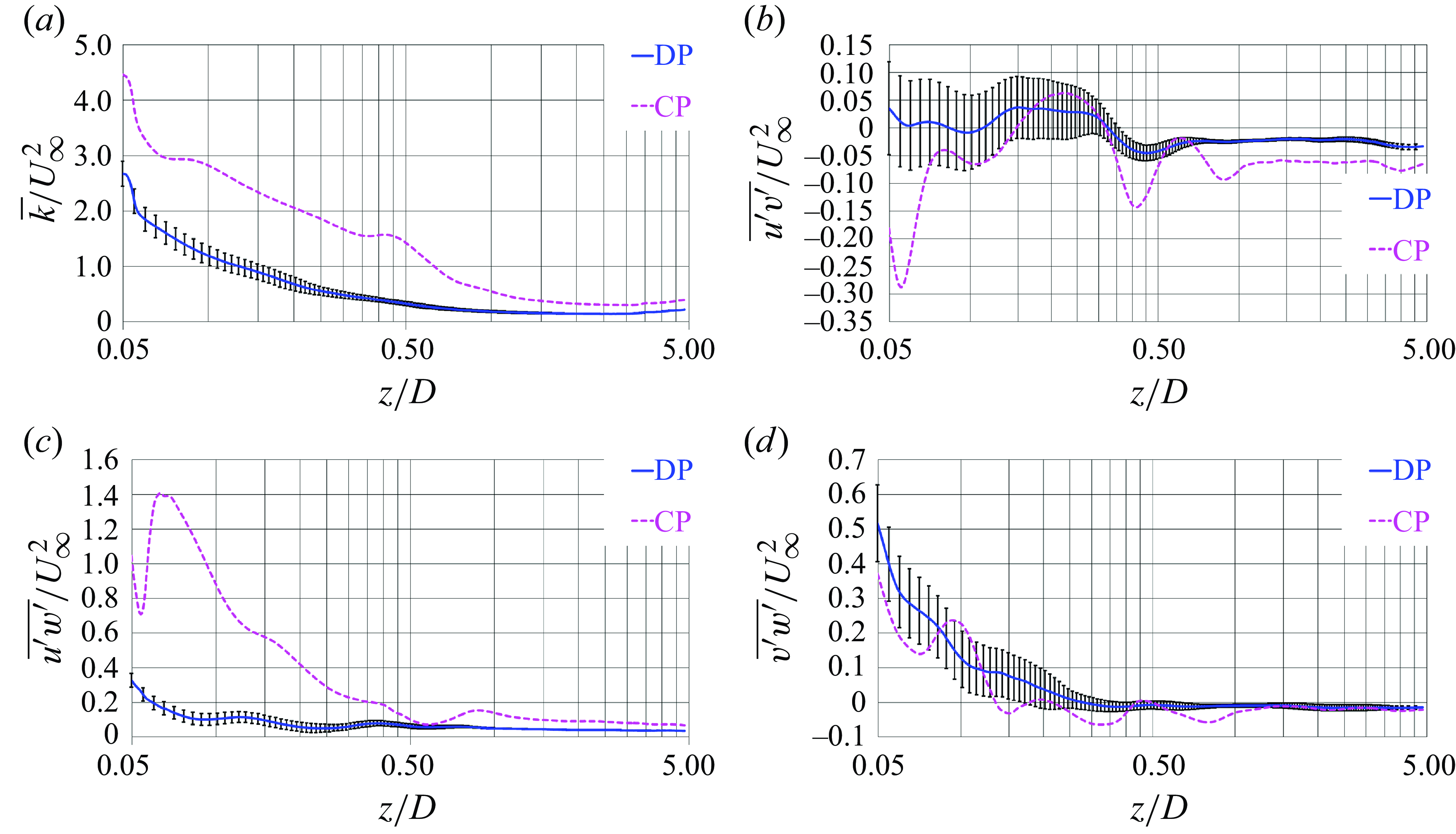
Contours of phase-averaged azimuthal vorticity on a meridian plane, scaled by $U_\infty /D$
: (a) ducted and (b) conventional propellers.
$U_\infty /D$
: (a) ducted and (b) conventional propellers.
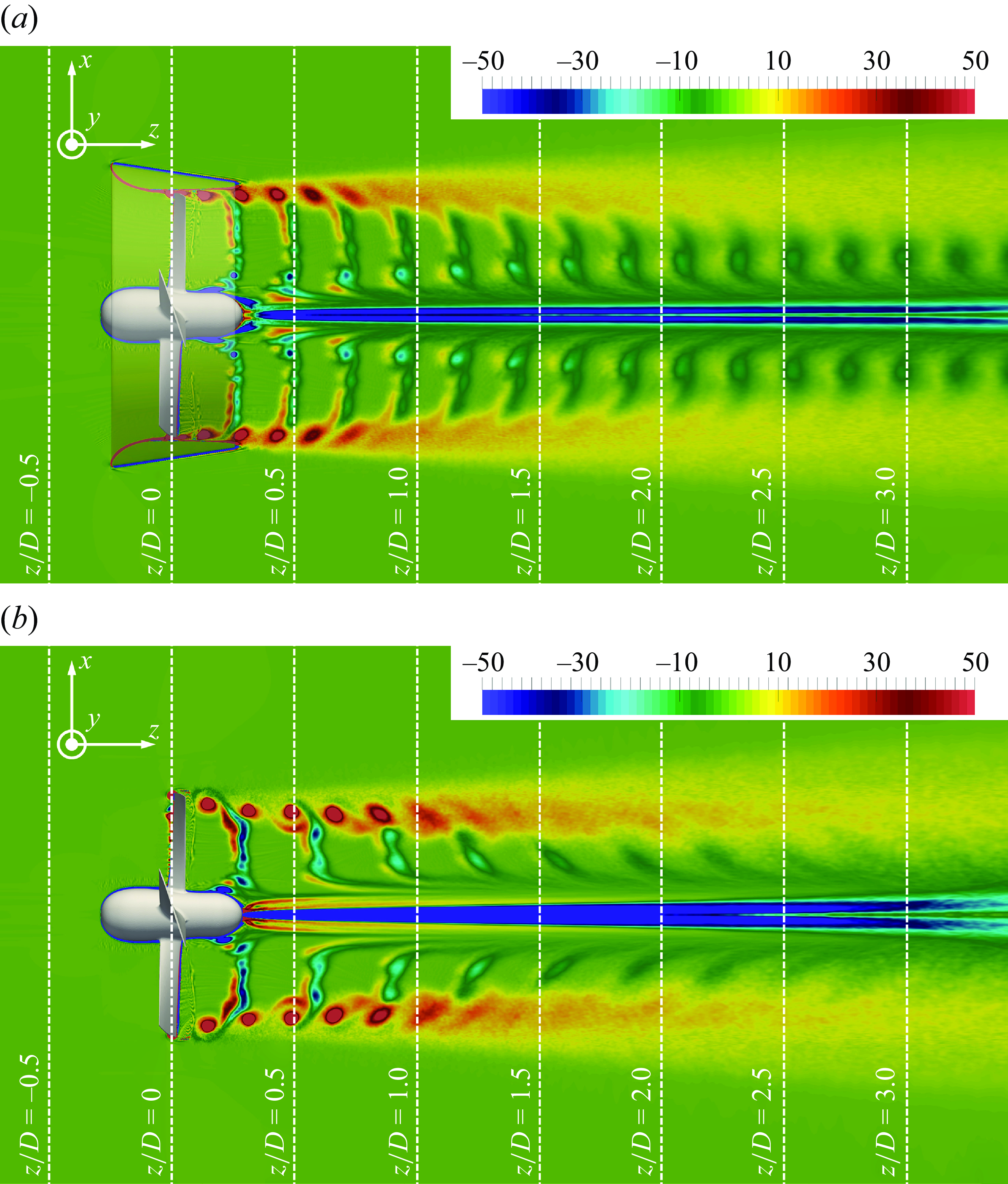
5.6. Phase-averaged statistics in the wake
Phase averages on a meridian plane are reported in figure 34 for the contours of azimuthal vorticity. They show that (i) the tip vortices shed by the conventional propeller keep coherent more downstream, compared with the tip leakage vortices from the ducted propeller; and (ii) the signature of the shear layers from the trailing edge of the propeller blades differs between the two cases, demonstrating that the action of the nozzle is able to modify the flow not only in the region of the tip of the blades, in agreement with the results seen in figure 14. This is attributable to the modification of the inflow conditions by the nozzle, increasing the suction generated by the propeller and decreasing the load on its blades, due to the shift of the actual advance coefficient towards higher values.
Contours of phase-averaged turbulent kinetic energy on a meridian plane, scaled by $U_\infty ^2$
: (a) ducted and (b) conventional propellers.
$U_\infty ^2$
: (a) ducted and (b) conventional propellers.

Contours of phase-averaged turbulent shear stresses downstream of the ducted propeller on a meridian plane, scaled by $U_\infty ^2$
: (a)
$U_\infty ^2$
: (a) $\widehat {u'v'}$
(b)
$\widehat {u'v'}$
(b) $\widehat {u'w'}$
and (c)
$\widehat {u'w'}$
and (c) $\widehat {v'w'}$
.
$\widehat {v'w'}$
.
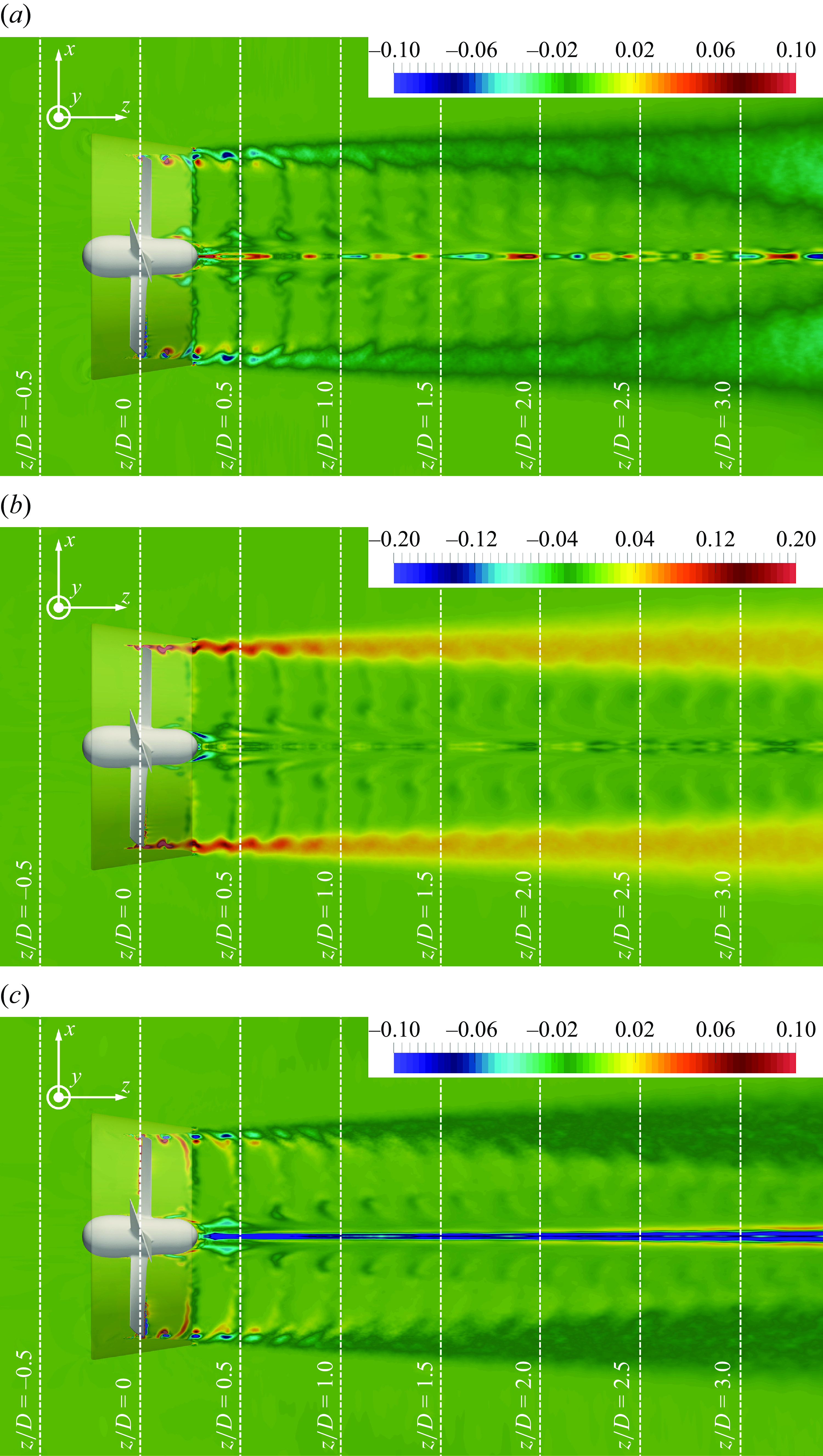
Contours of phase-averaged turbulent shear stresses downstream of the conventional propeller on a meridian plane, scaled by $U_\infty ^2$
: (a)
$U_\infty ^2$
: (a) $\widehat {u'v'}$
(b)
$\widehat {u'v'}$
(b) $\widehat {u'w'}$
and (c)
$\widehat {u'w'}$
and (c) $\widehat {v'w'}$
.
$\widehat {v'w'}$
.
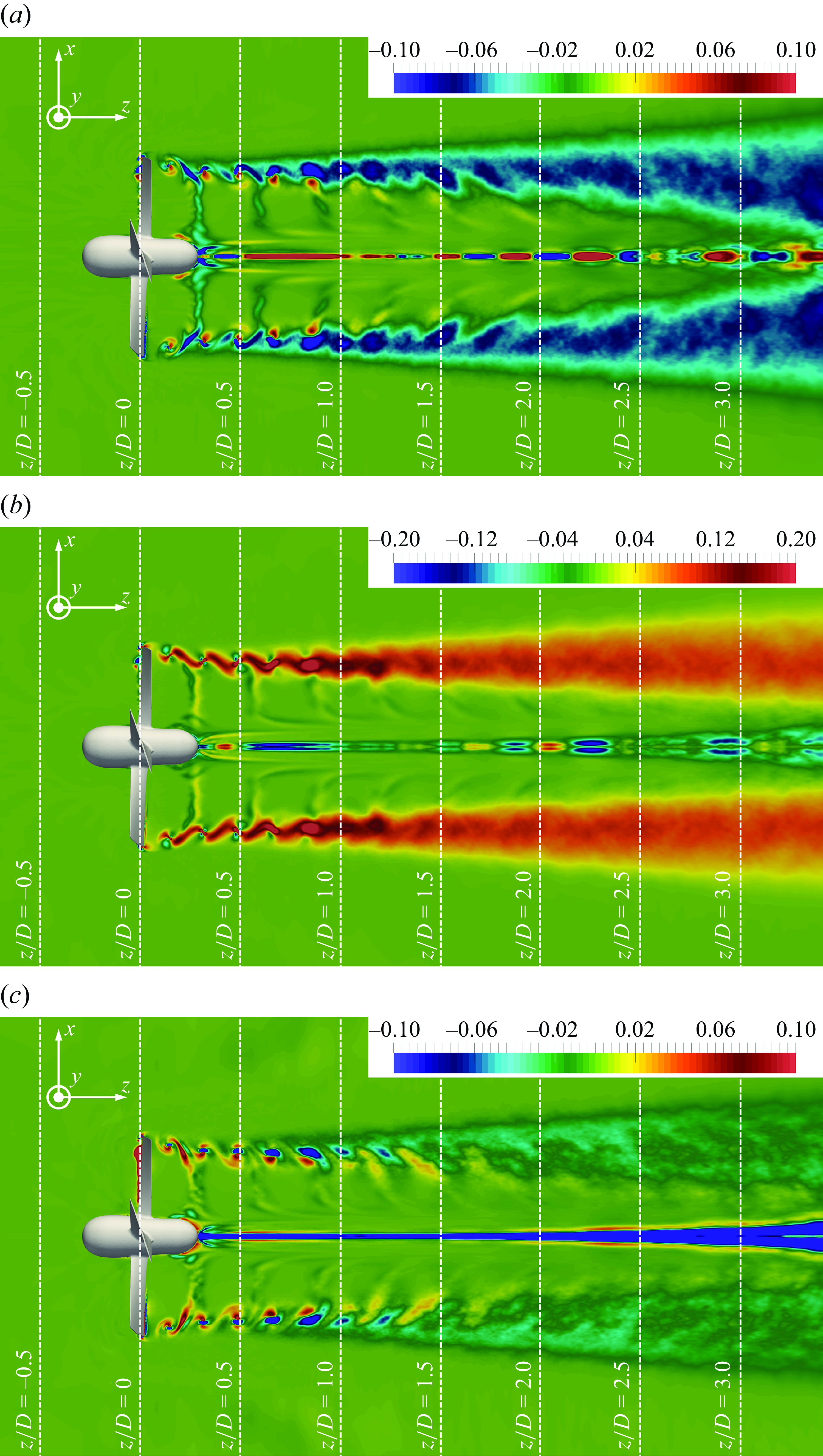
Contours of phase-averaged SGS shear stresses downstream of the ducted propeller on a meridian plane, scaled by $U_\infty ^2$
: (a)
$U_\infty ^2$
: (a) $\widehat {\tau }_{r \vartheta }$
(b)
$\widehat {\tau }_{r \vartheta }$
(b) $\widehat {\tau }_{r z}$
and (c)
$\widehat {\tau }_{r z}$
and (c) $\widehat {\tau }_{\vartheta z}$
.
$\widehat {\tau }_{\vartheta z}$
.
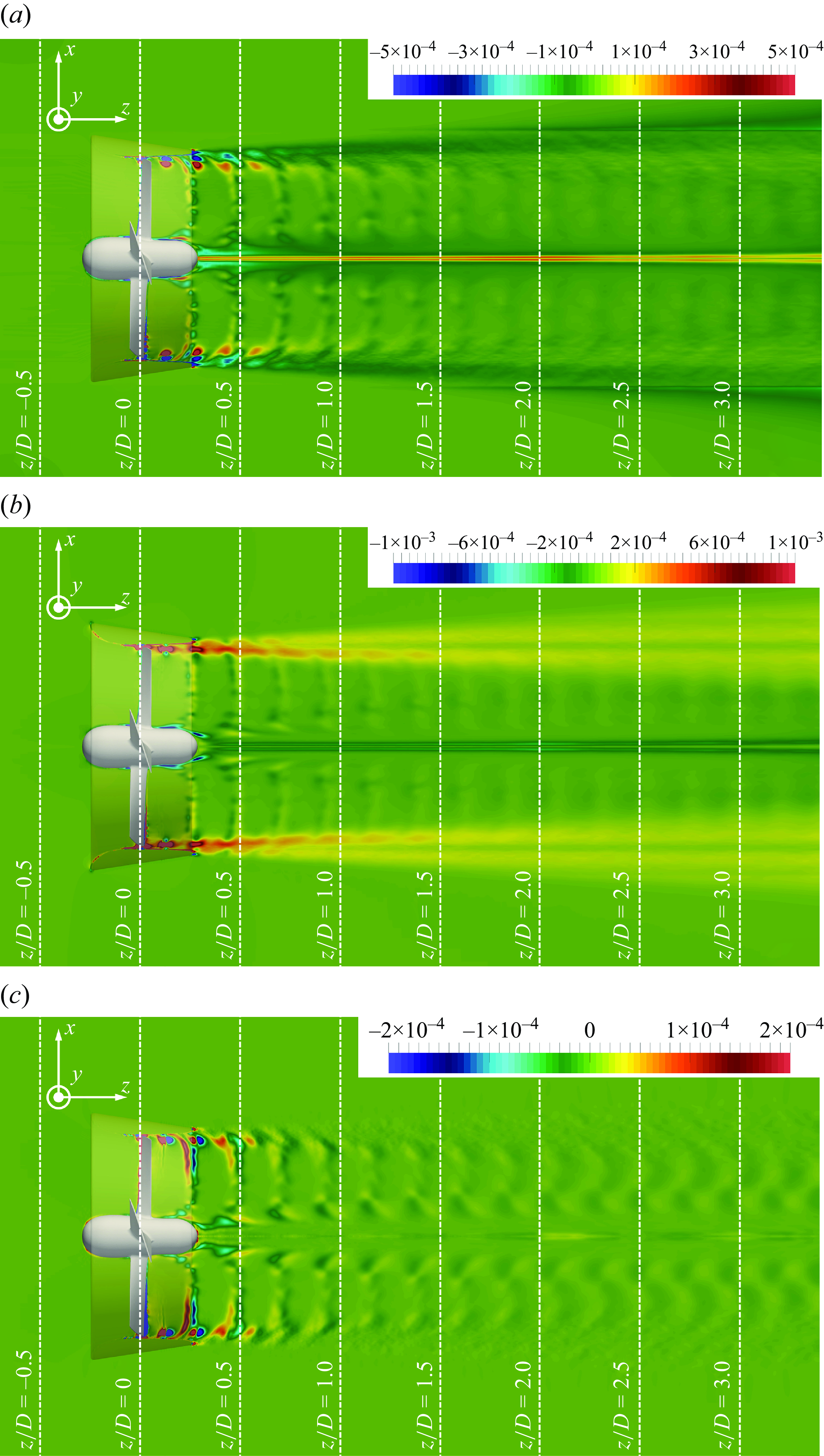
Contours of phase-averaged SGS shear stresses downstream of the conventional propeller on a meridian plane, scaled by $U_\infty ^2$
: (a)
$U_\infty ^2$
: (a) $\widehat {\tau }_{r \vartheta }$
(b)
$\widehat {\tau }_{r \vartheta }$
(b) $\widehat {\tau }_{r z}$
and (c)
$\widehat {\tau }_{r z}$
and (c) $\widehat {\tau }_{\vartheta z}$
.
$\widehat {\tau }_{\vartheta z}$
.
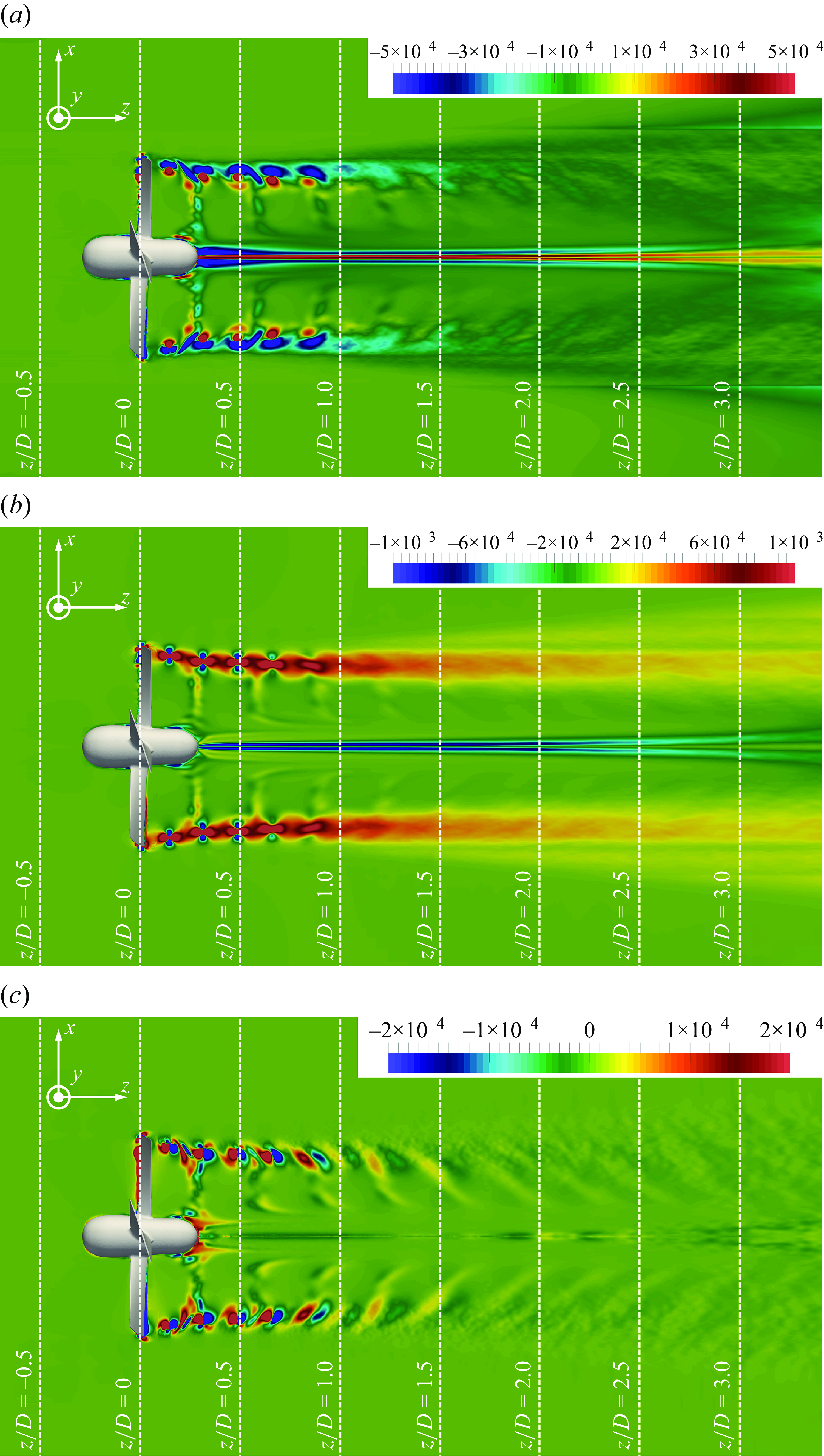
Contours of phase-averaged turbulent kinetic energy are illustrated in figure 35. The comparison between the cases of the two propellers actually differs from that in figure 25, dealing with the time-averaged turbulent kinetic energy: just downstream of the propeller plane the levels of turbulence at the outer boundary of the wake, populated by the tip leakage vortices of the ducted propeller and the tip vortices of the conventional propeller, are similar between the two cases. This is in contrast with the time-averaged statistics, which have shown higher turbulent stresses in the wake of the conventional propeller across the whole streamwise extent of the wake, due to the stronger intensity of its tip vortices, producing larger velocity fluctuations in the time-averaged statistics of the flow. However, deviations between values of phase-averaged turbulence become more obvious moving towards downstream coordinates, where turbulent kinetic energy is again higher at the outer boundary of the wake of the conventional propeller, because of the faster diffusion of the tip leakage vortices. A similar result is reported in figures 36 and 37 for the three phase-averaged shear stresses: across the near wake the maxima at the core of the tip vortices are similar between ducted and conventional propellers. Actually, the discussion in § 5.4, dealing with the detail of the flow just downstream of the propellers, demonstrated that the turbulent stress $\widehat {u'w'}$
in the region of shear between tip leakage vortices and the boundary layer on the nozzle is substantially higher than at the core of the tip vortices of the conventional propeller, producing a faster instability. However, the turbulent shear stresses are significantly higher downstream of the conventional propeller, compared with the ducted one, already at less than a diameter downstream. Again, the comparison with the modelled stresses in figures 38 and 39 is very clear in demonstrating that most turbulence is resolved. In agreement with the time-averaged statistics, also for the phase-averaged statistics the SGS stresses achieve values at least two orders of magnitude smaller than their resolved counterparts, as shown by the differences in the colour scales between figures 36, 37 and figures 38, 39.
$\widehat {u'w'}$
in the region of shear between tip leakage vortices and the boundary layer on the nozzle is substantially higher than at the core of the tip vortices of the conventional propeller, producing a faster instability. However, the turbulent shear stresses are significantly higher downstream of the conventional propeller, compared with the ducted one, already at less than a diameter downstream. Again, the comparison with the modelled stresses in figures 38 and 39 is very clear in demonstrating that most turbulence is resolved. In agreement with the time-averaged statistics, also for the phase-averaged statistics the SGS stresses achieve values at least two orders of magnitude smaller than their resolved counterparts, as shown by the differences in the colour scales between figures 36, 37 and figures 38, 39.
6. Conclusions
Large eddy simulation was adopted to compare the wake systems of ducted and conventional propellers in highly loaded conditions, with a special focus on their tip and tip leakage vortices. Computations were conducted on a cylindrical grid consisting of 3.5 billion points, by exploiting an IB methodology.
In agreement with the results in the literature, the computations verified a substantial change in the global performance of the ducted propeller, compared with the conventional one. The reduction of the torque coefficient was more significant than that of the thrust coefficient, resulting in an increase of the efficiency of propulsion of about $30\,\%$
. It is worth mentioning that the nozzle contributes to the thrust generated by the overall system, while its additional torque due to viscous effects is practically negligible. This dramatic change in performance was reflected in a substantial modification of the flow physics as well.
$30\,\%$
. It is worth mentioning that the nozzle contributes to the thrust generated by the overall system, while its additional torque due to viscous effects is practically negligible. This dramatic change in performance was reflected in a substantial modification of the flow physics as well.
The acceleration of the flow downstream of the ducted propeller was weaker, compared with the case of the conventional propeller, resulting in lower values of streamwise velocity in the wake and a more limited wake contraction. This result is in line with the smaller thrust produced by the blades of the ducted propeller, compensated in part by the thrust generated by its nozzle. The acceleration of the inflow, induced by the nozzle, increases the actual advance coefficient experienced by the propeller, shifting its working conditions to lower thrust and higher efficiency.
The tip vortices produced by the conventional propeller were more intense than the tip leakage vortices shed by the ducted propeller, as demonstrated by the stronger maxima of vorticity and minima of pressure coefficient at their cores. This was again the result of the lower load experienced by the blades of the ducted propeller. Therefore, also the peaks of turbulent stresses at the outer wake boundary, associated with the tip vortices from the conventional propeller, were more intense than those arising from the tip leakage vortices shed by the ducted propeller. The only exception was the region of streamwise coordinates just downstream of the propeller plane, where the phase-averaged turbulent stresses at the core of the tip and tip leakage vortices were found similar. This result was attributable to the shear developed between the tip leakage vortices and the boundary layer on the inner surface of the duct. As a consequence, the mechanism of instability of the tip leakage vortices was modified, if compared with that affecting the tip vortices of the conventional propeller. As discussed in detail by Felli et al. (Reference Felli, Camussi and Di Felice2011), for conventional propellers, the instability of their tip vortices is the result of phenomena of short- and long-wave instability, whose amplification leads eventually to mutual inductance between tip vortices, in agreement with the theoretical study on helical vortices by Widnall (Reference Widnall1972). These phenomena are also accelerated by the shear of the tip vortices with the trailing wake of the following blades (Posa et al. Reference Posa, Broglia and Balaras2019b , Reference Posa, Broglia and Balaras2022a ; Posa Reference Posa2022a ), since the latter is characterised by a larger pitch, that is, a larger angle relative to the azimuthal direction, moving downstream at a faster rate than the tip vortices. Therefore, the tip vortices shed by conventional propellers experience initially a stable helical trajectory, then undergo meandering and leapfrogging, leading eventually to breakup into smaller turbulent structures. For the tip leakage vortices shed by ducted propellers, these phenomena are bypassed and instability is accelerated, triggered by their shear with the boundary layer on the inner surface of the duct, rather than by their interaction with the trailing wake of the following blades and mutual inductance between tip leakage vortices.
We verified a dramatic change of both performance and wake physics, attributable to the nozzle. This demonstrated to be especially beneficial for the following reasons: (i) the efficiency of propulsion was substantially improved, (ii) the intensity of the major coherent structures was dramatically reduced and (iii) the coherence of the tip leakage vortices was disrupted more quickly. It is worth recalling that the tip vortices are areas of strong negative peaks of pressure, promoting the onset of cavitation phenomena, reinforcing the acoustic signature of the wake and negatively affecting the performance and structural integrity of downstream bodies, as rudders. Therefore, decreasing their intensity and disrupting their coherence is highly beneficial to marine propulsion. Further insight would be gained by considering in the analysis cavitation phenomena, which were not included in the present study. They are likely to reinforce the important deviations between the cases of ducted and non-ducted propellers already observed in this study. The comparisons we reported demonstrated that the minima of pressure achieved at the core of the tip vortices shed by the conventional propeller were roughly twice more intense than those at the core of the tip leakage vortices shed by the ducted propeller. As discussed above, this is the beneficial effect of decreasing the load on the propeller blades, which is moved in part to the nozzle, resulting in less intense tip leakage vortices. Therefore, the tip vortices of a conventional propeller are more prone to cavitation than the tip leakage vortices of a ducted propeller producing similar levels of thrust. It is well known that unsteady cavitation is the leading source of noise in non-wetted (cavitating) conditions. Therefore, these features of ducted propellers have the potential to make them less noisy. Furthermore, the recent LES studies by Cheng et al. (2019, 2020), reporting direct comparisons between cavitating and non-cavitating tip leakage vortices, revealed that cavitation promotes more turbulent production. Therefore, one can hypothesise that the inclusion of cavitation would reinforce the deviations between the turbulent stresses found at the core of the tip and tip leakage vortices, which in wetted conditions were found already higher in the former case. Meanwhile, it is likely that the onset of cavitation would decrease the effective area of passage of the flow through the tip gap region, increasing its velocity and shear with the inner surface of the nozzle and promoting a faster disruption of the coherence of the tip leakage vortices. In addition, the comparison between ducted and conventional propellers would benefit from an extension to the analysis of their acoustic signature. For instance, although the reduced intensity of the tip leakage vortices shed by ducted propellers is expected to be beneficial in decreasing the sound radiated from their wake, the shear developed between the tip leakage vortices and the inner surface of the duct is an additional source of sound. It would be important to shed light on the balance between these two phenomena in the hydroacoustics of ducted propellers. Therefore, in our future studies we plan to exploit the data generated by LES computations to reconstruct the acoustic fields of the two propellers and increasing the level of detail of the comparison between them.
Acknowledgements
We are grateful to Professor Lianzhou Wang at the School of Mechanics and Engineering of the Southwest Jiaotong University for providing the geometries of the propellers.
Funding
This study was funded by The National Recovery and Resilience Plan (NRRP), Mission 4, Component 2, Investment 1.4 “Strengthening research structures and creating R&D ‘national champions’ on specific key enabling technologies” funded by the European Union – NextGenerationEU, Code CN00000023: “Sustainable Mobility Center (Centro Nazionale per la Mobilità Sostenibile – CNMS)”.
Declaration of interests
The authors report no conflict of interest.


 Open access