


1 Introduction
Mean-field electrodynamics is an integral part of the theory of turbulent flows in electrically conducting fluids. Following its pioneering formulation using the second-order smoothing approximation (SOCA) (Steenbeck, Krause & Rädler Reference Steenbeck, Krause and Rädler1966; Krause & Rädler Reference Krause and Rädler1980), the mean-field induction equation has been derived using a wide variety of approximations. Essentially the same equation is obtained when the assumptions of SOCA are relaxed, most importantly, the assumptions of scale separation between the mean and random magnetic fields and of a short velocity correlation time (Dittrich et al.
Reference Dittrich, Molchanov, Sokoloff and Ruzmaikin1984; Zeldovich et al.
Reference Zeldovich, Molchanov, Ruzmaikin and Sokoloff1988; Molchanov Reference Molchanov1991; Brandenburg & Subramanian Reference Brandenburg and Subramanian2005). The robustness of this theory to differing assumptions suggests its relevance and reliability. However, confidence in the theoretical basis of mean-field electrodynamics has been shaken by direct numerical simulations of mean-field dynamo action in driven and convective flows. Comparisons of such simulations with theory remain inconclusive (e.g. Favier & Bushby Reference Favier and Bushby2013, and references therein). One of the possible reasons for that is the complexity of the random flows that drive the dynamo: they are often compressible, anisotropic and non-Gaussian, and the mean magnetic field may not be as symmetric as is often assumed (e.g. unidirectional or axially symmetric). However, analyses of the simulation results rarely allow for such complications. This is, perhaps, not surprising, since the known theory of random fields has been formulated almost exclusively for Gaussian random fields and their close relatives such as log–normal or $\unicode[STIX]{x1D712}^{2}$
fields. Techniques applicable to strongly non-Gaussian random fields are few and not widely known.
$\unicode[STIX]{x1D712}^{2}$
fields. Techniques applicable to strongly non-Gaussian random fields are few and not widely known.
Motivated by the present difficulties experienced by comparisons between the theory and numerical simulations of mean-field dynamos, we focus upon one particular aspect of this problem: developing diagnostics of strongly non-Gaussian random fields that can be used to make quantitative comparisons between different data sets. The significance of such techniques extends beyond mean-field electrodynamics, as the need to compare sophisticated numerical simulations with experiments or observations of natural phenomena is common to many areas of physics. This is particularly true in astrophysics, where modern telescopes generate observational data at very high spatial resolution. With ever-increasing computer power, simulations of astrophysical processes are attaining greater levels of realism. Of particular interest is the notion of a topological comparison, which (in this context) assesses whether or not the connectivity of particular structures in simulations match those of the observations. It is clearly more difficult to quantify topology than it is to measure the standard statistics such as mean values, correlation functions of various orders, etc. However, a crucial advantage of topological methods is their generality and freedom from restrictive and often unjustifiable assumptions, such as the assumption of Gaussian statistics.
(a) The isocontours of the H i number density $n$
(in atom
$n$
(in atom $~\text{cm}^{-3}$
) from the Galactic All Sky Survey (Kalberla et al.
Reference Kalberla2010) at
$~\text{cm}^{-3}$
) from the Galactic All Sky Survey (Kalberla et al.
Reference Kalberla2010) at $R=10~\text{kpc}$
,
$R=10~\text{kpc}$
, $202.9^{\circ }\leqslant \unicode[STIX]{x1D719}\leqslant 208.6^{\circ }$
,
$202.9^{\circ }\leqslant \unicode[STIX]{x1D719}\leqslant 208.6^{\circ }$
, $|z|\leqslant 1.1~\text{kpc}$
, with
$|z|\leqslant 1.1~\text{kpc}$
, with $(R,\unicode[STIX]{x1D719},z)$
the galactocentric cylindrical coordinates with the Sun at
$(R,\unicode[STIX]{x1D719},z)$
the galactocentric cylindrical coordinates with the Sun at $(R,\unicode[STIX]{x1D719},z)=(8.5~\text{kpc},180^{\circ },0)$
. The horizontal extent of the image is approximately
$(R,\unicode[STIX]{x1D719},z)=(8.5~\text{kpc},180^{\circ },0)$
. The horizontal extent of the image is approximately $1~\text{kpc}$
, its resolution is close to
$1~\text{kpc}$
, its resolution is close to $17~\text{pc}$
. (b) The isocontours of the gas number density
$17~\text{pc}$
. (b) The isocontours of the gas number density $n$
(in atom
$n$
(in atom $~\text{cm}^{-3}$
) in a vertical plane, obtained from a three-dimensional magnetohydrodynamic simulation of Gent et al. (Reference Gent, Shukurov, Fletcher, Sarson and Mantere2013a
,Reference Gent, Shukurov, Sarson, Fletcher and Mantere
b
) at a resolution of
$~\text{cm}^{-3}$
) in a vertical plane, obtained from a three-dimensional magnetohydrodynamic simulation of Gent et al. (Reference Gent, Shukurov, Fletcher, Sarson and Mantere2013a
,Reference Gent, Shukurov, Sarson, Fletcher and Mantere
b
) at a resolution of $4~\text{pc}$
. White areas in both panels correspond to low density values,
$4~\text{pc}$
. White areas in both panels correspond to low density values, $n<3\times 10^{-3}~\text{cm}^{-3}$
on (a) and
$n<3\times 10^{-3}~\text{cm}^{-3}$
on (a) and $5\times 10^{-4}~\text{cm}^{-3}$
on (b).
$5\times 10^{-4}~\text{cm}^{-3}$
on (b).

The morphology of a random field, which can be measured using tools such as the Minkowski functionals, quantifies the shape of structures in the data. Morphological analysis has been applied to a wide range of problems, including magnetohydrodynamic (MHD) simulations (Wilkin, Barenghi & Shukurov Reference Wilkin, Barenghi and Shukurov2007), the interstellar medium (Makarenko, Fletcher & Shukurov Reference Makarenko, Fletcher and Shukurov2015) and cosmology (Mecke, Buchert & Wagner Reference Mecke, Buchert and Wagner1994). Topological and morphological methods characterize different properties of a random field, without relying on assumptions of Gaussianity, and should be viewed as complementary steps in producing a more complete representation than that provided by standard statistical descriptors. One should bear in mind, however, that topological or morphological similarity does not necessarily imply that the underlying physics of two systems is the same. For example, it might be possible for two flows to be topologically similar but be driven by very different mechanisms. There is scope (and need) for work that seeks to connect topology and morphology more directly to physical processes.
We focus on the distribution of hydrogen atoms (H i) in the Milky Way, obtained from recent observations (see Kalberla et al.
Reference Kalberla2010). The specific observable is the volume number density, $n$
, measured in a galactocentric cylindrical coordinate system
$n$
, measured in a galactocentric cylindrical coordinate system $(R,\unicode[STIX]{x1D719},z)$
, where
$(R,\unicode[STIX]{x1D719},z)$
, where $R$
is the distance in the galactic plane from the centre of the Galaxy,
$R$
is the distance in the galactic plane from the centre of the Galaxy, $\unicode[STIX]{x1D719}$
represents the azimuthal angle in the galactic plane (with the Sun at
$\unicode[STIX]{x1D719}$
represents the azimuthal angle in the galactic plane (with the Sun at $\unicode[STIX]{x1D719}=180^{\circ }$
) and
$\unicode[STIX]{x1D719}=180^{\circ }$
) and $z$
is the vertical distance from the mid-plane of the galactic disc. Figure 1(a) represents a two-dimensional (2-D) cross-section of
$z$
is the vertical distance from the mid-plane of the galactic disc. Figure 1(a) represents a two-dimensional (2-D) cross-section of $n(\unicode[STIX]{x1D719},z)$
, at galactocentric radius
$n(\unicode[STIX]{x1D719},z)$
, at galactocentric radius $R=10~\text{kpc}$
(which is close to the Sun), in the region
$R=10~\text{kpc}$
(which is close to the Sun), in the region $202.9^{\circ }\leqslant \unicode[STIX]{x1D719}\leqslant 208.6^{\circ }$
and
$202.9^{\circ }\leqslant \unicode[STIX]{x1D719}\leqslant 208.6^{\circ }$
and $|z|\leqslant 1.1~\text{kpc}$
. Note that the density field is not the projected density along the entire line of sight (also called the surface or column density). Doppler shifts of the H i spectral line, along with a model rotation curve for the Galaxy, allow the observations to be separated into volume densities on a series of 2-D cylindrical cross-sections. The method is described in Burton (Reference Burton, Kellermann and Verschuur1988). The spatial extent of this region is approximately
$|z|\leqslant 1.1~\text{kpc}$
. Note that the density field is not the projected density along the entire line of sight (also called the surface or column density). Doppler shifts of the H i spectral line, along with a model rotation curve for the Galaxy, allow the observations to be separated into volume densities on a series of 2-D cylindrical cross-sections. The method is described in Burton (Reference Burton, Kellermann and Verschuur1988). The spatial extent of this region is approximately $1\times 2~\text{kpc}$
, chosen for ease of comparison with existing simulations. Interstellar gas is involved in transonic MHD turbulence that supports the mean-field dynamo action (e.g. Shukurov Reference Shukurov, Dormy and Soward2007) recently reproduced in direct numerical simulations (Gressel et al.
Reference Gressel, Elstner, Ziegler and Rüdiger2008; Gent et al.
Reference Gent, Shukurov, Fletcher, Sarson and Mantere2013a
,Reference Gent, Shukurov, Sarson, Fletcher and Mantere
b
; Bendre, Gressel & Elstner Reference Bendre, Gressel and Elstner2015).
$1\times 2~\text{kpc}$
, chosen for ease of comparison with existing simulations. Interstellar gas is involved in transonic MHD turbulence that supports the mean-field dynamo action (e.g. Shukurov Reference Shukurov, Dormy and Soward2007) recently reproduced in direct numerical simulations (Gressel et al.
Reference Gressel, Elstner, Ziegler and Rüdiger2008; Gent et al.
Reference Gent, Shukurov, Fletcher, Sarson and Mantere2013a
,Reference Gent, Shukurov, Sarson, Fletcher and Mantere
b
; Bendre, Gressel & Elstner Reference Bendre, Gressel and Elstner2015).
Figure 1(b) shows a snapshot of the gas density distribution in a numerical simulation of the multiphase interstellar medium in the solar neighbourhood. The model describes supernova-driven random flow in the interstellar gas, with gravity and differential rotation, including the effects of radiative cooling, photoelectric heating and various transport processes (see Gent et al.
Reference Gent, Shukurov, Fletcher, Sarson and Mantere2013a
,Reference Gent, Shukurov, Sarson, Fletcher and Mantere
b
, for more details). The spatial extent of the computational domain is $1~\text{kpc}\times 1~\text{kpc}$
horizontally and
$1~\text{kpc}\times 1~\text{kpc}$
horizontally and $2~\text{kpc}$
vertically, symmetric about the galactic mid-plane, so the simulation domain is comparable in size to the region shown on figure 1(a). Note that the magnitude of the gas density is not directly comparable to the corresponding H i density (which is only one component of the interstellar gas, although it does make up the majority of the gas). There are, however, some clear qualitative similarities between the simulation and the observations, notably the form of the higher density regions near the mid-plane. The question is: how well does the model describe reality?
$2~\text{kpc}$
vertically, symmetric about the galactic mid-plane, so the simulation domain is comparable in size to the region shown on figure 1(a). Note that the magnitude of the gas density is not directly comparable to the corresponding H i density (which is only one component of the interstellar gas, although it does make up the majority of the gas). There are, however, some clear qualitative similarities between the simulation and the observations, notably the form of the higher density regions near the mid-plane. The question is: how well does the model describe reality?
An initial inspection of the data shown in figure 1 immediately reveals three possible problems that may hinder meaningful comparisons. First, as mentioned above, the range of the gas densities in the observed and simulated fields in figure 1 differ; the mean and the standard deviation of the gas densities in the two fields are different too. The observed mean gas density is $\langle n\rangle =0.065~\text{atom}~\text{cm}^{-3}$
and its standard deviation
$\langle n\rangle =0.065~\text{atom}~\text{cm}^{-3}$
and its standard deviation $\unicode[STIX]{x1D70E}_{n}=0.063~\text{atom}~\text{cm}^{-3}$
. In the simulation,
$\unicode[STIX]{x1D70E}_{n}=0.063~\text{atom}~\text{cm}^{-3}$
. In the simulation, $\langle n\rangle =0.220$
and
$\langle n\rangle =0.220$
and $\unicode[STIX]{x1D70E}_{n}=0.349~\text{atom}~\text{cm}^{-3}$
. These values can also vary quite strongly from snapshot to snapshot in a simulation and from slice to slice in the real data. The data need to be standardized before their statistical properties are compared. Second, both the observed and simulated data have a strong trend in the vertical direction – the gas density is higher at
$\unicode[STIX]{x1D70E}_{n}=0.349~\text{atom}~\text{cm}^{-3}$
. These values can also vary quite strongly from snapshot to snapshot in a simulation and from slice to slice in the real data. The data need to be standardized before their statistical properties are compared. Second, both the observed and simulated data have a strong trend in the vertical direction – the gas density is higher at $z=0$
and gets lower as
$z=0$
and gets lower as $|z|$
increases. Does the presence of trends influence the comparison and, if so, how can this be mitigated? Given that it can often be difficult to separate trends from turbulent fluctuations, can we find methods of analysis that are insensitive to large-scale trends in the data? Third, the image resolutions are different – the simulated data have four times higher resolution than the observation. The standard approach to this problem would be to reduce the resolution of the simulation to that of the observation. However, this may lose important information. A better approach would be to select methods of analysis that are independent of the image resolution. We will show that topological data analysis meets these requirements.
$|z|$
increases. Does the presence of trends influence the comparison and, if so, how can this be mitigated? Given that it can often be difficult to separate trends from turbulent fluctuations, can we find methods of analysis that are insensitive to large-scale trends in the data? Third, the image resolutions are different – the simulated data have four times higher resolution than the observation. The standard approach to this problem would be to reduce the resolution of the simulation to that of the observation. However, this may lose important information. A better approach would be to select methods of analysis that are independent of the image resolution. We will show that topological data analysis meets these requirements.
Over the last decade, topological approaches have been widely applied to the analysis of random fields (Carlsson Reference Carlsson2009; Adler et al. Reference Adler, Bobrowski, Borman, Subag, Weinberger, Berger, Cai and Johnstone2010; Adler & Taylor Reference Adler and Taylor2011; Edelsbrunner Reference Edelsbrunner2014; Yogeshwaran & Adler Reference Yogeshwaran and Adler2015). Topological invariants, such as the Betti numbers, and the associated techniques of persistence diagrams and barcodes, rank functions and persistence landscapes, as well as persistence images for random fields, have been applied in cosmology (Gay et al. Reference Gay, Pichon, Le Borgne, Teyssier, Sousbie and Devriendt2010; Sousbie Reference Sousbie2011; Sousbie, Pichon & Kawahara Reference Sousbie, Pichon and Kawahara2011; Pranav Reference Pranav2015; Pranav et al. Reference Pranav, Edelsbrunner, van de Weygaert, Vegter, Kerber, Jones and Wintraecken2017) and are beginning to be used in fluid dynamics (Kramár et al. Reference Kramár, Levanger, Tithof, Suri, Xu, Paul, Schatz and Mischaikow2016), solar magnetohydrodynamics (Makarenko, Karimova & Novak Reference Makarenko, Karimova and Novak2007; Makarenko et al. Reference Makarenko, Malkova, Machin, Knyazeva and Makarenko2014; Kniazeva, Makarenko & Urtiev Reference Kniazeva, Makarenko and Urtiev2015; Knyazeva, Makarenko & Urtiev Reference Knyazeva, Makarenko and Urtiev2015; Knyazeva et al. Reference Knyazeva, Makarenko, Kuperin and Dmitrieva2016; Knyazeva, Urtiev & Makarenko Reference Knyazeva, Urtiev and Makarenko2017) and astrophysics (Li et al. Reference Li, Urquhart, Leurini, Csengeri, Wyrowski, Menten and Schuller2016; Henderson et al. Reference Henderson, Makarenko, Bushby, Fletcher and Shukurov2017; Makarenko et al. Reference Makarenko, Shukurov, Henderson, Rodrigues, Bushby and Fletcher2018).
Complex topological diagnostics, such as persistence landscapes (Bubenik Reference Bubenik2015; Bubenik & Dłotko Reference Bubenik and Dłotko2017), rank functions (Robins & Turner Reference Robins and Turner2016), persistence images (Adams et al. Reference Adams, Emerson, Kirby, Neville, Peterson, Shipman, Chepushtanova, Hanson, Motta and Ziegelmeier2017), are difficult to interpret in physical terms; they are often not robust and work well with idealized image textures rather than more irregular patterns. The bottleneck distance (Cohen-Steiner, Edelsbrunner & Harer Reference Cohen-Steiner, Edelsbrunner and Harer2007) as a measure of similarity between persistence diagrams, is often inefficient in astrophysical and other applications (see, e.g. Makarenko et al. Reference Makarenko, Shukurov, Henderson, Rodrigues, Bushby and Fletcher2018). We found that simpler statistics can be more efficient when applied to real data (Henderson et al. Reference Henderson, Makarenko, Bushby, Fletcher and Shukurov2017). In this paper, we discuss topological data analysis (TDA) for random fields and identify simple, yet efficient topological statistics. We informally describe what topological filtration is, how to use it for comparison and classification of different scalar fields, and how stable the results are. Section 2 describes the topological filtration of functions and its representation in the form of persistence diagrams. We show two different ways to represent a persistence diagram and introduce statistics that we have found useful for distinguishing between one-dimensional signals and fields in two dimensions. In § 3 we discuss a standardization of fields, which makes comparisons more reliable. Section 4 focuses on topology in the presence of large-scale trends. In § 5, we investigate how the results of topological filtration depend on the image resolution. In § 6 we apply some of the TDA methods to observations and numerical simulations of the ISM and summarize the key principles for the practical application of TDA in § 7.
2 Topological filtration and persistence diagrams
In this section we present the basic ideas of topological filtration along with some useful topological statistics. Our aim here is to develop these topological ideas at an intuitive level. Rigorous definitions can be found, for example, in Morozov (Reference Morozov2008), Adler et al. (Reference Adler, Bobrowski, Borman, Subag, Weinberger, Berger, Cai and Johnstone2010), Edelsbrunner & Harer (Reference Edelsbrunner and Harer2010), Adler & Taylor (Reference Adler and Taylor2011), Edelsbrunner (Reference Edelsbrunner2014), Toth, O’Rourke & Goodman (Reference Toth, O’Rourke and Goodman2017), while Ghrist (Reference Ghrist2008), Park et al. (Reference Park, Pranav, Chingangbam, van de Weygaert, Jones, Vegter, Kim, Hidding and Hellwing2013), Pranav et al. (Reference Pranav, Edelsbrunner, van de Weygaert, Vegter, Kerber, Jones and Wintraecken2017) and Motta (Reference Motta and Tsonis2018) also provide useful and less formal expositions.
2.1 Topological filtration
Consider a random function $f(\boldsymbol{x})$
defined in a domain
$f(\boldsymbol{x})$
defined in a domain $M$
. Suppose that
$M$
. Suppose that $f(\boldsymbol{x})$
is smooth, so that its extrema are critical points,
$f(\boldsymbol{x})$
is smooth, so that its extrema are critical points, $\unicode[STIX]{x1D735}f(\boldsymbol{x})=0$
. (We note that continuity is sufficient in many applications.) We first introduce sublevel sets (e.g. Edelsbrunner & Harer Reference Edelsbrunner, Harer, Goodman, Pach and Pollack2008), those regions where the values of a random function
$\unicode[STIX]{x1D735}f(\boldsymbol{x})=0$
. (We note that continuity is sufficient in many applications.) We first introduce sublevel sets (e.g. Edelsbrunner & Harer Reference Edelsbrunner, Harer, Goodman, Pach and Pollack2008), those regions where the values of a random function $f(\boldsymbol{x})$
are below a certain threshold
$f(\boldsymbol{x})$
are below a certain threshold $h$
. The sublevel set is defined as
$h$
. The sublevel set is defined as
 $$\begin{eqnarray}A_{h}=\{\boldsymbol{x}\in M:f(\boldsymbol{x})\leqslant h\}.\end{eqnarray}$$
A sequence of levels $h_{1}\leqslant h_{2}\leqslant \cdots \,$
generates a nested family of sublevel sets of
$h_{1}\leqslant h_{2}\leqslant \cdots \,$
generates a nested family of sublevel sets of $f$
,
$f$
, $A_{1}\subseteq A_{2}\subseteq \,\cdots$
, which is called the sublevel set filtration of
$A_{1}\subseteq A_{2}\subseteq \,\cdots$
, which is called the sublevel set filtration of $f(\boldsymbol{x})$
.
$f(\boldsymbol{x})$
.
Each sublevel set has certain topological properties that we wish to characterize. When $\dim (A_{h})=1$
(i.e.
$\dim (A_{h})=1$
(i.e. $f$
is a function of one variable), the topology is characterized by the Betti number
$f$
is a function of one variable), the topology is characterized by the Betti number $\unicode[STIX]{x1D6FD}_{0}$
that counts the number of connected components. When
$\unicode[STIX]{x1D6FD}_{0}$
that counts the number of connected components. When $\dim (A_{h})=2$
, the topological properties are the number of connected components,
$\dim (A_{h})=2$
, the topological properties are the number of connected components, $\unicode[STIX]{x1D6FD}_{0}$
, and the number of holes in them (more precisely, loops whose interiors are the holes),
$\unicode[STIX]{x1D6FD}_{0}$
, and the number of holes in them (more precisely, loops whose interiors are the holes), $\unicode[STIX]{x1D6FD}_{1}$
. In three dimensions, in addition to components and tunnels (loops), voids can appear (i.e. hollow spaces bounded by closed surfaces), which are counted by
$\unicode[STIX]{x1D6FD}_{1}$
. In three dimensions, in addition to components and tunnels (loops), voids can appear (i.e. hollow spaces bounded by closed surfaces), which are counted by $\unicode[STIX]{x1D6FD}_{2}$
. Connected components, loops or tunnels, and closed shells are also referred to as cycles of dimension 0, 1 and 2, respectively. The alternating sum of the Betti numbers is a wider known topological quantity, the Euler characteristic,
$\unicode[STIX]{x1D6FD}_{2}$
. Connected components, loops or tunnels, and closed shells are also referred to as cycles of dimension 0, 1 and 2, respectively. The alternating sum of the Betti numbers is a wider known topological quantity, the Euler characteristic,
 $$\begin{eqnarray}\unicode[STIX]{x1D712}=\mathop{\sum }_{k=0}^{N-1}(-1)^{k}\unicode[STIX]{x1D6FD}_{k},\end{eqnarray}$$
where $N$
is the dimension of
$N$
is the dimension of $M$
.
$M$
.
Equivalent results can be obtained by considering superlevel sets, defined as
 $$\begin{eqnarray}A_{h}=\{\boldsymbol{x}\in M:f(\boldsymbol{x})\geqslant h\}.\end{eqnarray}$$
The transition from the sublevel to superlevel sets only interchanges the Betti numbers $\unicode[STIX]{x1D6FD}_{0}$
and
$\unicode[STIX]{x1D6FD}_{0}$
and $\unicode[STIX]{x1D6FD}_{1}$
in two dimensions, and
$\unicode[STIX]{x1D6FD}_{1}$
in two dimensions, and $\unicode[STIX]{x1D6FD}_{0}$
and
$\unicode[STIX]{x1D6FD}_{0}$
and $\unicode[STIX]{x1D6FD}_{2}$
in three dimensions. For the rest of the paper we will only discuss the sublevel set filtration.
$\unicode[STIX]{x1D6FD}_{2}$
in three dimensions. For the rest of the paper we will only discuss the sublevel set filtration.
The Betti numbers are topological invariants, i.e. they are not affected by translations, rotations and continuous deformations of the space. In a typical astrophysical application, where we deal with random fields, the components represent matter clumps or clouds, the loops are closed chains of matter and the shells surround regions of reduced density (voids).
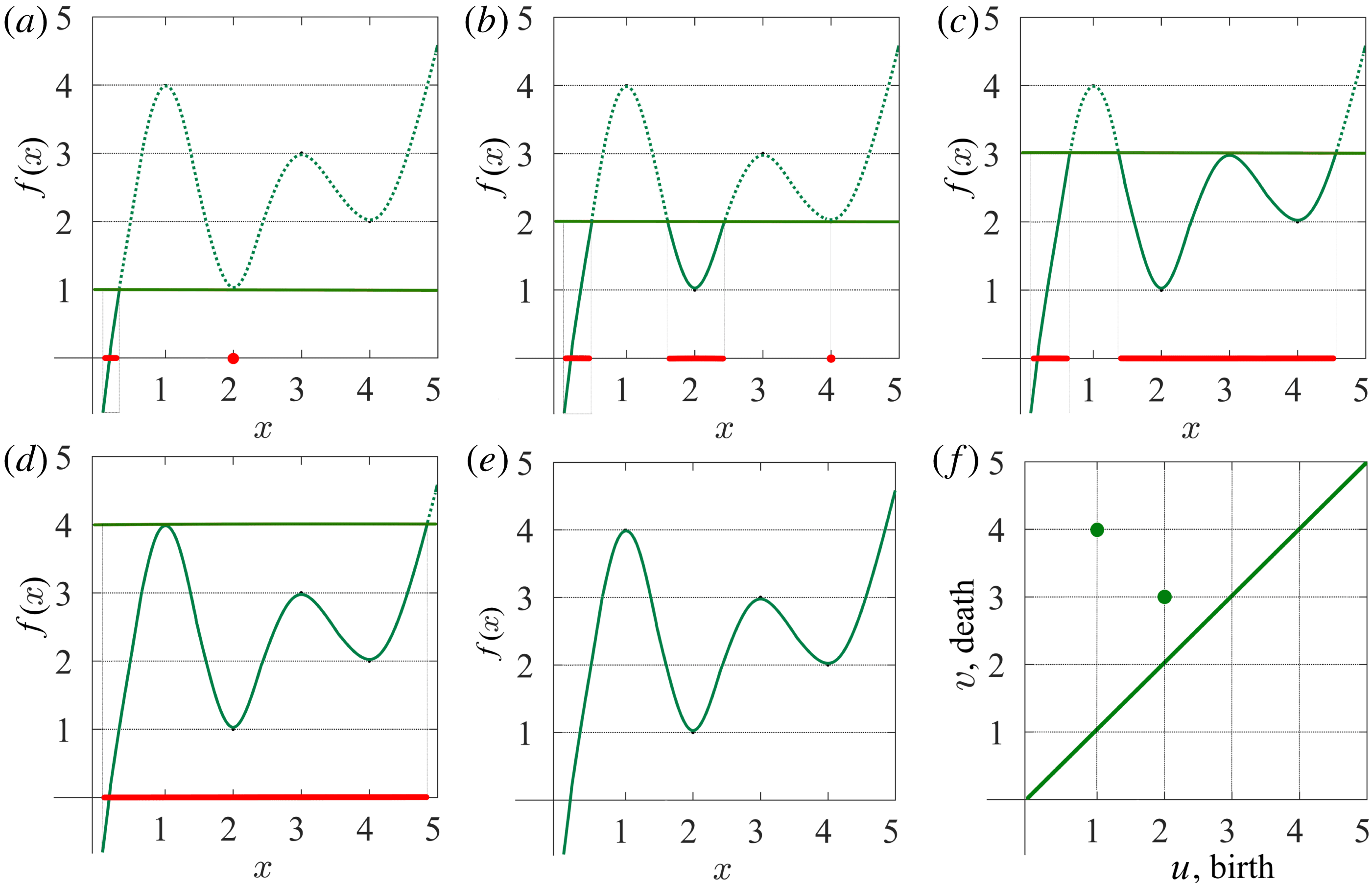
(a–d) Sublevel set filtration of a function of one variable (e) and the resulting persistence diagram (f). The horizontal green line indicates the increasing threshold $h$
; the values of the function
$h$
; the values of the function $f(x)\leqslant h$
are shown in a solid line, while
$f(x)\leqslant h$
are shown in a solid line, while $f(x)>h$
in a dotted line. On each panel the sublevel set at a fixed
$f(x)>h$
in a dotted line. On each panel the sublevel set at a fixed $h$
is shown as the red intervals on the
$h$
is shown as the red intervals on the $x$
axis. The number of red intervals corresponds to a number of connected components,
$x$
axis. The number of red intervals corresponds to a number of connected components, $\unicode[STIX]{x1D6FD}_{0}$
, at this level.
$\unicode[STIX]{x1D6FD}_{0}$
, at this level.
2.2 Topological filtration of a function of one variable
It is easiest to demonstrate a sublevel set filtration in one dimension; this will allow us to develop some analogies and intuition about the method. We therefore consider the behaviour of a random function with reference to a threshold level $h$
, considering the values of
$h$
, considering the values of $x$
where
$x$
where $f(x)\leqslant h$
. Figure 2 provides an example of this technique. As we vary the level
$f(x)\leqslant h$
. Figure 2 provides an example of this technique. As we vary the level $h$
, the number of components in
$h$
, the number of components in $A_{h}$
, shown as red intervals on the
$A_{h}$
, shown as red intervals on the $x$
axis, changes. When
$x$
axis, changes. When $h<1$
the corresponding sublevel set contains one component, an interval around
$h<1$
the corresponding sublevel set contains one component, an interval around $x=0.3$
, and so
$x=0.3$
, and so $\unicode[STIX]{x1D6FD}_{0}=1$
. At
$\unicode[STIX]{x1D6FD}_{0}=1$
. At $h=1$
a new component appears, a point at
$h=1$
a new component appears, a point at $x=2$
, which implies that
$x=2$
, which implies that $\unicode[STIX]{x1D6FD}_{0}=2$
at this level. When we reach
$\unicode[STIX]{x1D6FD}_{0}=2$
at this level. When we reach $h=2$
one more component is born, at
$h=2$
one more component is born, at $x=4$
, and so
$x=4$
, and so $\unicode[STIX]{x1D6FD}_{0}=3$
. At
$\unicode[STIX]{x1D6FD}_{0}=3$
. At $h=3$
, the second and the third components merge and
$h=3$
, the second and the third components merge and $\unicode[STIX]{x1D6FD}_{0}=2$
again. According to the (so-called) Elder Rule, the merger of two components results in the death of the younger one, i.e. the component that was born later. In this particular case, the third component, which appeared at
$\unicode[STIX]{x1D6FD}_{0}=2$
again. According to the (so-called) Elder Rule, the merger of two components results in the death of the younger one, i.e. the component that was born later. In this particular case, the third component, which appeared at $h=2$
, dies at
$h=2$
, dies at $h=3$
, merging with the second one. Finally, the first and the second components merge at
$h=3$
, merging with the second one. Finally, the first and the second components merge at $h=4$
, which results in
$h=4$
, which results in $\unicode[STIX]{x1D6FD}_{0}=1$
. We could continue to increase
$\unicode[STIX]{x1D6FD}_{0}=1$
. We could continue to increase $h$
, until this component also dies, if the function was defined in a wider range of
$h$
, until this component also dies, if the function was defined in a wider range of $x$
. Note that at each local minimum the sublevel set gains a new component, while at a local maximum, two components merge into one. Functions of one variable can also contain inflection points, but these do not change the configuration of the sublevel sets.
$x$
. Note that at each local minimum the sublevel set gains a new component, while at a local maximum, two components merge into one. Functions of one variable can also contain inflection points, but these do not change the configuration of the sublevel sets.
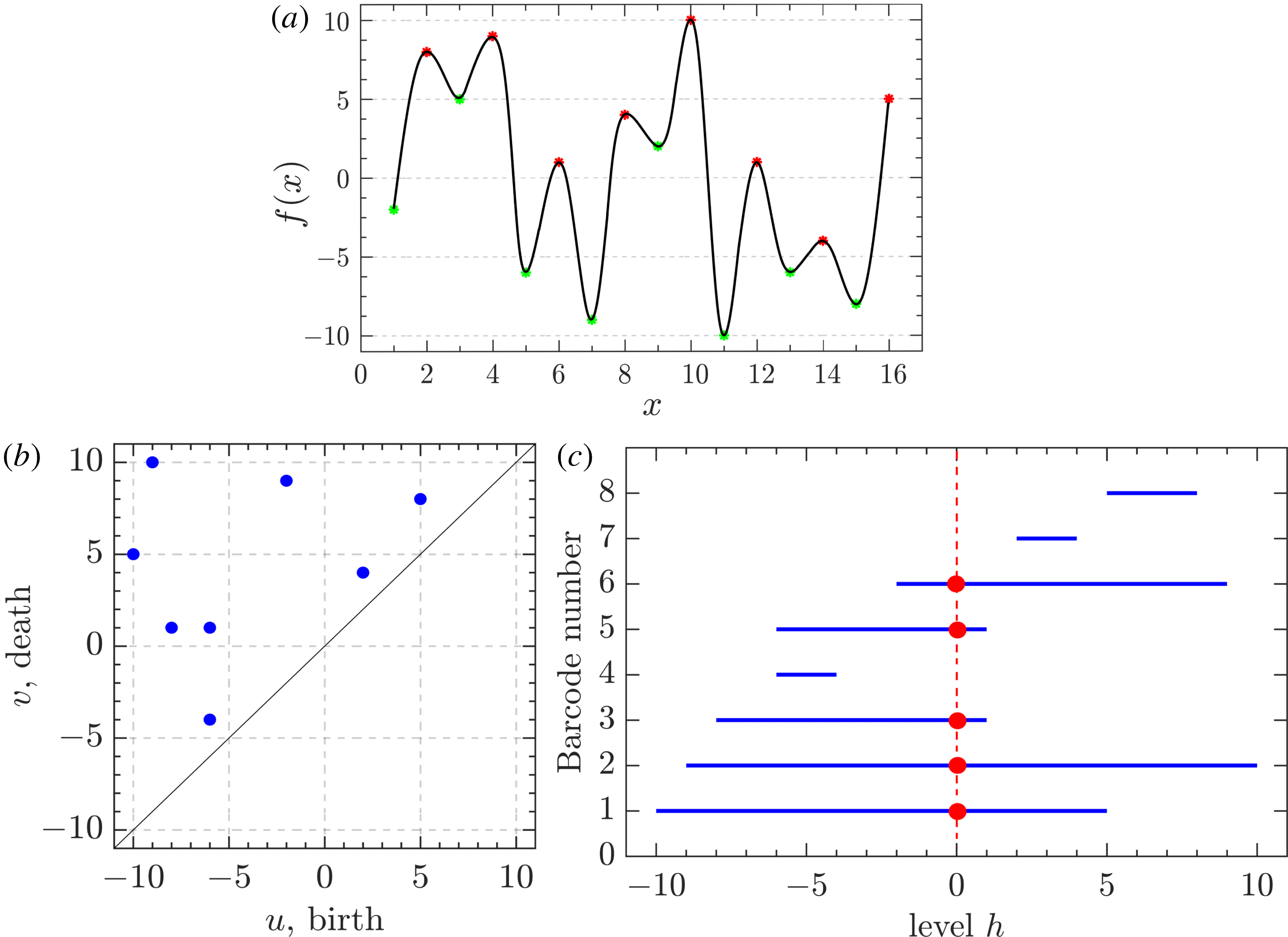
(a) A Gaussian random function $y=f(x)$
, with the minima marked as green points, and the maxima as red ones. (b) The persistence diagram obtained as the result of sublevel set filtration of this function. Every point corresponds to one persistent pair
$y=f(x)$
, with the minima marked as green points, and the maxima as red ones. (b) The persistence diagram obtained as the result of sublevel set filtration of this function. Every point corresponds to one persistent pair $(u_{i},v_{i})$
,
$(u_{i},v_{i})$
, $i=1,\ldots ,8$
. (c) One more way to illustrate the result of topological filtration of
$i=1,\ldots ,8$
. (c) One more way to illustrate the result of topological filtration of $f$
is to plot pairs
$f$
is to plot pairs $(u_{i},v_{i})$
as a sequence of barcodes, horizontal lines
$(u_{i},v_{i})$
as a sequence of barcodes, horizontal lines $u_{i}\leqslant h\leqslant v_{i}$
, one for each component. The red vertical line in (c) corresponds to the threshold value
$u_{i}\leqslant h\leqslant v_{i}$
, one for each component. The red vertical line in (c) corresponds to the threshold value $h=0$
. This line intercepts five out of the eight barcodes, which means there are five components at this level:
$h=0$
. This line intercepts five out of the eight barcodes, which means there are five components at this level: $\unicode[STIX]{x1D6FD}_{0}=5$
. The total length
$\unicode[STIX]{x1D6FD}_{0}=5$
. The total length $L_{T}$
of these barcodes is equal to 61. As will be demonstrated below,
$L_{T}$
of these barcodes is equal to 61. As will be demonstrated below, $L_{T}(h)$
is a useful statistic for comparison of random functions.
$L_{T}(h)$
is a useful statistic for comparison of random functions.
The filtration process illustrated in figure 2 captures and quantifies the topology of the sublevel sets. Tracing the varying sublevel sets as a function of threshold $h$
, the topology remains static, or persists, between the critical points of
$h$
, the topology remains static, or persists, between the critical points of $f(x)$
, and changes only when
$f(x)$
, and changes only when $h$
reaches a critical point. The lifetime, or persistence of a component is defined as
$h$
reaches a critical point. The lifetime, or persistence of a component is defined as $v-u$
, where
$v-u$
, where $u$
is the level at which the component appears (its birth), and
$u$
is the level at which the component appears (its birth), and $v$
is the level at which it disappears (its death). This is therefore simply a measure of the range of levels
$v$
is the level at which it disappears (its death). This is therefore simply a measure of the range of levels $h$
over which this component exists. Topological filtration of a function results in a list of values
$h$
over which this component exists. Topological filtration of a function results in a list of values $(u,v)$
, one pair for each component, and these can be plotted in the
$(u,v)$
, one pair for each component, and these can be plotted in the $(u,v)$
-plane to obtain what is called a persistence diagram. For our example, the events of birth and death of the components are displayed on the persistence diagram in figure 2(f). Zero persistence corresponds to the diagonal line on the diagram; the most persistent components are those that are furthest from the diagonal.
$(u,v)$
-plane to obtain what is called a persistence diagram. For our example, the events of birth and death of the components are displayed on the persistence diagram in figure 2(f). Zero persistence corresponds to the diagonal line on the diagram; the most persistent components are those that are furthest from the diagonal.
Thus, topological filtration identifies critical points of a random function, pairs them and isolates those that correspond to its most significant (persistent) features. This represents topological properties of the function in terms of a relatively small number of quantifiable variables.
2.3 Presenting the results of filtration: persistence diagrams and barcodes
Figure 3(a) shows a small part of the realization of a $\unicode[STIX]{x1D6FF}$
-correlated Gaussian random process,
$\unicode[STIX]{x1D6FF}$
-correlated Gaussian random process, $f(x)$
, which has a mean of zero and a standard deviation of 6.6. The result of the sublevel set filtration of
$f(x)$
, which has a mean of zero and a standard deviation of 6.6. The result of the sublevel set filtration of $f(x)$
is a
$f(x)$
is a $2\times m$
array where each of the
$2\times m$
array where each of the $m$
pairs
$m$
pairs $(u_{i},v_{i})$
represents the birth,
$(u_{i},v_{i})$
represents the birth, $u_{i}$
, and the death,
$u_{i}$
, and the death, $v_{i}$
, of the
$v_{i}$
, of the $i$
-th component,
$i$
-th component, $i=1,\ldots ,m$
. For the range of
$i=1,\ldots ,m$
. For the range of $x$
shown, the number of such pairs is
$x$
shown, the number of such pairs is $m=8$
. Figure 3(b) is the persistence diagram obtained from the topological filtration of the function shown in figure 3(a) derived as described above. The persistence pairs
$m=8$
. Figure 3(b) is the persistence diagram obtained from the topological filtration of the function shown in figure 3(a) derived as described above. The persistence pairs $(u_{i},v_{i})$
can also be represented as a sequence of barcodes, as shown in figure 3(c), where every point of the persistence diagram is shown as a horizontal bar extended between its birth and death levels. The bars are sorted, from the bottom up, according to when they first appear in the filtration process (which is also bottom up).
$(u_{i},v_{i})$
can also be represented as a sequence of barcodes, as shown in figure 3(c), where every point of the persistence diagram is shown as a horizontal bar extended between its birth and death levels. The bars are sorted, from the bottom up, according to when they first appear in the filtration process (which is also bottom up).
Since the number of components depends on the size of the domain, it is useful to normalize the Betti numbers to unit length, area or volume as appropriate. We found that different random functions can be usefully compared by considering the dependence of the Betti numbers per unit length, area or volume on the level $h$
, normalized to the unit area under the curve. The variation of the total length of the barcodes,
$h$
, normalized to the unit area under the curve. The variation of the total length of the barcodes,
 $$\begin{eqnarray}L_{T}=\mathop{\sum }_{i=1}^{m}(v_{i}-u_{i}),\end{eqnarray}$$
also normalized to unit area under the curves, also turns out to be a useful diagnostic. The barcode length can be conveniently expressed in terms of the standard deviation of $f(x)$
. These statistics make the result of topological filtration independent of the size of the data set and some are also insensitive to the presence of a large-scale trend and the resolution of the data: we demonstrate these valuable properties in §§ 4 and 5.
$f(x)$
. These statistics make the result of topological filtration independent of the size of the data set and some are also insensitive to the presence of a large-scale trend and the resolution of the data: we demonstrate these valuable properties in §§ 4 and 5.
Topological filtration of a continuous, smooth, 2-D Gaussian scalar field, $f(x,y)$
(colour coded with the colour bar in (f)), which has a vanishing mean value, unit standard deviation, and an autocorrelation function
$f(x,y)$
(colour coded with the colour bar in (f)), which has a vanishing mean value, unit standard deviation, and an autocorrelation function $C(l)=\exp [-l^{2}/(2L^{2})]$
, where
$C(l)=\exp [-l^{2}/(2L^{2})]$
, where $L\approx 15$
. Sublevel sets, i.e. regions where
$L\approx 15$
. Sublevel sets, i.e. regions where $f(x,y)\leqslant h$
, are shown for increasing values of
$f(x,y)\leqslant h$
, are shown for increasing values of $h$
: (a)
$h$
: (a) $h=-1.5$
, (b)
$h=-1.5$
, (b) $h=-1.48$
, (c)
$h=-1.48$
, (c) $h=0.2$
, (d)
$h=0.2$
, (d) $h=0.6$
and (e)
$h=0.6$
and (e) $h=0.72$
. The components (C) and holes (H) are labelled in (a–e) as described in the text. (g,h) Show how the components merge and the holes split as the level
$h=0.72$
. The components (C) and holes (H) are labelled in (a–e) as described in the text. (g,h) Show how the components merge and the holes split as the level $h$
changes. (f) Presents the full range of
$h$
changes. (f) Presents the full range of $f(x,y)$
.
$f(x,y)$
.

2.4 Topological filtration of a 2-D field
The topological filtration and related techniques can straightforwardly be generalized to multi-dimensional scalar random fields but they are easier described at an intuitive level in two dimensions where the Betti numbers $\unicode[STIX]{x1D6FD}_{0}$
and
$\unicode[STIX]{x1D6FD}_{0}$
and $\unicode[STIX]{x1D6FD}_{1}$
are defined. Consider a continuous random function
$\unicode[STIX]{x1D6FD}_{1}$
are defined. Consider a continuous random function $f(x,y)$
defined in a finite domain, and its isocontour at a level
$f(x,y)$
defined in a finite domain, and its isocontour at a level $h$
, i.e. a curve in the
$h$
, i.e. a curve in the $(x,y)$
-plane where
$(x,y)$
-plane where $f=h$
. The set of points
$f=h$
. The set of points $(x,y)$
where
$(x,y)$
where $f\leqslant h$
is the sublevel set. We vary
$f\leqslant h$
is the sublevel set. We vary $h$
from smaller to larger values and record the number of components (clouds) and holes in the isocontours at each level together with the values of
$h$
from smaller to larger values and record the number of components (clouds) and holes in the isocontours at each level together with the values of $h$
where the components and holes appear and disappear. As in one dimension, the isocontours can also be scanned down from larger to smaller values of
$h$
where the components and holes appear and disappear. As in one dimension, the isocontours can also be scanned down from larger to smaller values of $h$
: this does not affect the results. The transition from the sublevel sets to superlevel sets swaps the persistent diagrams of
$h$
: this does not affect the results. The transition from the sublevel sets to superlevel sets swaps the persistent diagrams of $\unicode[STIX]{x1D6FD}_{0}$
and
$\unicode[STIX]{x1D6FD}_{0}$
and $\unicode[STIX]{x1D6FD}_{1}$
(in two dimensions). Here, we use the sublevel sets, i.e. scan
$\unicode[STIX]{x1D6FD}_{1}$
(in two dimensions). Here, we use the sublevel sets, i.e. scan $f(x,y)$
up from smaller to larger values.
$f(x,y)$
up from smaller to larger values.
When the level $h$
reaches the lowest value of
$h$
reaches the lowest value of $f$
in the domain, the first component emerges as illustrated in figure 4. Each local minimum of
$f$
in the domain, the first component emerges as illustrated in figure 4. Each local minimum of $f$
adds a new component when it is reached by the increasing isocontour level
$f$
adds a new component when it is reached by the increasing isocontour level $h$
. Two (or more) components can merge, when
$h$
. Two (or more) components can merge, when $h$
increases, if they are connected by a valley (that necessarily contains a saddle point); then the labelling convention is that the younger component (i.e. that formed at a larger
$h$
increases, if they are connected by a valley (that necessarily contains a saddle point); then the labelling convention is that the younger component (i.e. that formed at a larger $h$
) dies whereas the older one continues to exist. Two components merge when the isocontour contains a saddle point, see figure 4(g); three components merge, when
$h$
) dies whereas the older one continues to exist. Two components merge when the isocontour contains a saddle point, see figure 4(g); three components merge, when $h$
passes through a monkey saddle (a degenerate critical point with a local minimum along one direction and inflection point in another, as opposed to the ordinary saddle with a minimum in one direction and maximum in another). Three (or more) components can merge, when there are three (or more) saddle points at the same level
$h$
passes through a monkey saddle (a degenerate critical point with a local minimum along one direction and inflection point in another, as opposed to the ordinary saddle with a minimum in one direction and maximum in another). Three (or more) components can merge, when there are three (or more) saddle points at the same level $h$
. The components can merge to form a loop whose interior is a hole; each hole at a level
$h$
. The components can merge to form a loop whose interior is a hole; each hole at a level $h$
surrounds a local maximum of
$h$
surrounds a local maximum of $f$
that is reached at some higher level. Holes are born when a loop is formed and die when
$f$
that is reached at some higher level. Holes are born when a loop is formed and die when $h$
passes through the corresponding local maximum of
$h$
passes through the corresponding local maximum of $f$
. Holes can split up at a saddle point, in which case the labelling convention is to ascribe the original birth time to the hole with the larger eventual local maximum, and deem the current level to be the birth time of the second hole. Figure 4(h) illustrates this.
$f$
. Holes can split up at a saddle point, in which case the labelling convention is to ascribe the original birth time to the hole with the larger eventual local maximum, and deem the current level to be the birth time of the second hole. Figure 4(h) illustrates this.
It is then clear that the birth and death of components and holes are intrinsically related to the nature of, and connections between, the stationary points of the random field (its extrema and saddles) and to the values of $f$
at those points. Betti numbers contain rich information about the random function. Eventually, as
$f$
at those points. Betti numbers contain rich information about the random function. Eventually, as $h$
approaches the absolute maximum of
$h$
approaches the absolute maximum of $f$
in the domain, only one, most persistent component remains (and no holes). Therefore,
$f$
in the domain, only one, most persistent component remains (and no holes). Therefore, $\unicode[STIX]{x1D6FD}_{0}=1$
and
$\unicode[STIX]{x1D6FD}_{0}=1$
and $\unicode[STIX]{x1D6FD}_{1}=0$
at levels
$\unicode[STIX]{x1D6FD}_{1}=0$
at levels $h$
exceeding the absolute maximum of
$h$
exceeding the absolute maximum of $f$
in the domain. The lifetime, or persistence, of a component or a hole is characterized by the range of
$f$
in the domain. The lifetime, or persistence, of a component or a hole is characterized by the range of $h$
where it exists. Selecting only those features that are more persistent, one distils a simplified (and therefore, better manageable) topological portrait of the random field.
$h$
where it exists. Selecting only those features that are more persistent, one distils a simplified (and therefore, better manageable) topological portrait of the random field.
Figure 4 illustrates the topological filtration of a two-dimensional random field using sublevel sets $f(x,y)\leqslant h$
, where
$f(x,y)\leqslant h$
, where $h$
is the level altitude. Figure 4(f) shows a realization a continuous, smooth, 2-D Gaussian scalar field,
$h$
is the level altitude. Figure 4(f) shows a realization a continuous, smooth, 2-D Gaussian scalar field, $f(x,y)$
, of in a domain of
$f(x,y)$
, of in a domain of $100^{2}$
pixels in size, which has a vanishing mean value, unit standard deviation, and an autocorrelation function
$100^{2}$
pixels in size, which has a vanishing mean value, unit standard deviation, and an autocorrelation function $C(l)=\exp [-l^{2}/(2L^{2})]$
with
$C(l)=\exp [-l^{2}/(2L^{2})]$
with $L\approx 15$
.
$L\approx 15$
.
The absolute minimum of the field, $f=-2.57$
, occurs at
$f=-2.57$
, occurs at $(x,y)=(31,18)$
. Thus, the first component C1 is born at
$(x,y)=(31,18)$
. Thus, the first component C1 is born at $h=-2.57$
and there are no holes at this level: we have
$h=-2.57$
and there are no holes at this level: we have $\unicode[STIX]{x1D6FD}_{0}=1$
and
$\unicode[STIX]{x1D6FD}_{0}=1$
and $\unicode[STIX]{x1D6FD}_{1}=0$
at
$\unicode[STIX]{x1D6FD}_{1}=0$
at $h=-2.57$
. As
$h=-2.57$
. As $h$
increases, more components are born. At
$h$
increases, more components are born. At $h=-1.5$
, panel (a), there are four components C1–C4 and no holes:
$h=-1.5$
, panel (a), there are four components C1–C4 and no holes: $\unicode[STIX]{x1D6FD}_{0}=4$
and
$\unicode[STIX]{x1D6FD}_{0}=4$
and $\unicode[STIX]{x1D6FD}_{1}=0$
. At
$\unicode[STIX]{x1D6FD}_{1}=0$
. At $h=-1.48$
, panel (b), components C1 and C4 have merged via a saddle point between them, passed through at a smaller
$h=-1.48$
, panel (b), components C1 and C4 have merged via a saddle point between them, passed through at a smaller $h$
; the surviving component is labelled C1 whereas C4 has died as it was born later than C1. There are no holes at
$h$
; the surviving component is labelled C1 whereas C4 has died as it was born later than C1. There are no holes at $h=-1.48$
:
$h=-1.48$
: $\unicode[STIX]{x1D6FD}_{0}=3$
and
$\unicode[STIX]{x1D6FD}_{0}=3$
and $\unicode[STIX]{x1D6FD}_{1}=0$
. At a higher level
$\unicode[STIX]{x1D6FD}_{1}=0$
. At a higher level $h=0.2$
, shown in panel (c), most of the components are merged into a big island, and there are three smaller islands, C5, C6 and C7, in the bottom half of the panel; moreover, one hole H1 appeared:
$h=0.2$
, shown in panel (c), most of the components are merged into a big island, and there are three smaller islands, C5, C6 and C7, in the bottom half of the panel; moreover, one hole H1 appeared: $\unicode[STIX]{x1D6FD}_{0}=4$
and
$\unicode[STIX]{x1D6FD}_{0}=4$
and $\unicode[STIX]{x1D6FD}_{1}=1$
. At a level
$\unicode[STIX]{x1D6FD}_{1}=1$
. At a level $h=0.6$
, panel (d), the number of components is 2,
$h=0.6$
, panel (d), the number of components is 2, $\unicode[STIX]{x1D6FD}_{0}=2$
; and one more hole H2 has appeared,
$\unicode[STIX]{x1D6FD}_{0}=2$
; and one more hole H2 has appeared, $\unicode[STIX]{x1D6FD}_{1}=1$
. At a higher level
$\unicode[STIX]{x1D6FD}_{1}=1$
. At a higher level $h=0.72$
, panel (e), all components have merged into a single island,
$h=0.72$
, panel (e), all components have merged into a single island, $\unicode[STIX]{x1D6FD}_{0}=1$
. There are two holes labelled H2 and H3, each around a local maximum of
$\unicode[STIX]{x1D6FD}_{0}=1$
. There are two holes labelled H2 and H3, each around a local maximum of $f$
, so
$f$
, so $\unicode[STIX]{x1D6FD}_{1}=2$
. Note that some holes (bordering on the field frame) have not yet completely formed and are not taken into account as holes. There are six such cases in panel (e). The holes H1 and H2, which surround the maximum lower than
$\unicode[STIX]{x1D6FD}_{1}=2$
. Note that some holes (bordering on the field frame) have not yet completely formed and are not taken into account as holes. There are six such cases in panel (e). The holes H1 and H2, which surround the maximum lower than $f=0.72$
, have already died (contracted).
$f=0.72$
, have already died (contracted).
3 Advantages of data standardization in topological filtration
In this section we describe a procedure for standardizing 1-D signals and 2-D fields. This preprocessing simplifies the comparison of the results of topological filtration that have been applied to different data. For example, one of our main motivations is to compare the topology of astronomical observations and numerical simulations: standardizing the data ensures a natural non-dimensionalization of the data and allows us to focus on their more subtle properties. We will use 1-D examples to show how data standardization affects persistence diagrams.
Signal standardization affects persistence diagrams. (a) A signal $f(x)$
of (3.2) (the solid blue line), and its shifted
$f(x)$
of (3.2) (the solid blue line), and its shifted $f_{1}=f+10$
(dashed red) and scaled
$f_{1}=f+10$
(dashed red) and scaled $f_{2}=3f$
versions (dash-dotted green). The persistence diagrams of (b)
$f_{2}=3f$
versions (dash-dotted green). The persistence diagrams of (b) $f$
(circles) and
$f$
(circles) and $f_{1}$
(crosses), and (c)
$f_{1}$
(crosses), and (c) $f$
(circles) and
$f$
(circles) and $f_{2}$
(triangles). (d) The persistence diagrams of the signals
$f_{2}$
(triangles). (d) The persistence diagrams of the signals $f$
,
$f$
, $f_{1}$
and
$f_{1}$
and $f_{2}$
coincide when they are standardized.
$f_{2}$
coincide when they are standardized.

For a random function $f(x)$
, its mean value and standard deviation are denoted
$f(x)$
, its mean value and standard deviation are denoted $\langle f\rangle$
and
$\langle f\rangle$
and $\unicode[STIX]{x1D70E}_{f}$
, respectively. We introduce a standardized version of
$\unicode[STIX]{x1D70E}_{f}$
, respectively. We introduce a standardized version of $f(x)$
as
$f(x)$
as
 $$\begin{eqnarray}\tilde{f}=\frac{f-\langle f\rangle }{\unicode[STIX]{x1D70E}_{f}},\end{eqnarray}$$
so that $\langle \tilde{f}\rangle =0$
and
$\langle \tilde{f}\rangle =0$
and $\unicode[STIX]{x1D70E}_{\tilde{f}}=1$
.
$\unicode[STIX]{x1D70E}_{\tilde{f}}=1$
.
Figure 5(a) shows the graphs of three related functions. The first one, shown in solid blue, is
 $$\begin{eqnarray}f(x)=5\sin (x)+12\cos (0.2x),\end{eqnarray}$$
with $\langle f\rangle =-1.32$
and
$\langle f\rangle =-1.32$
and $\unicode[STIX]{x1D70E}_{f}=8.75$
. The first term represents a higher-frequency fluctuation superimposed on a lower-frequency trend. The second one is
$\unicode[STIX]{x1D70E}_{f}=8.75$
. The first term represents a higher-frequency fluctuation superimposed on a lower-frequency trend. The second one is $f_{1}=f+10$
(dashed red), and the third is
$f_{1}=f+10$
(dashed red), and the third is $f_{2}=3f$
(dash-dotted green). The blue dots in figure 5(b) is the persistence diagram of
$f_{2}=3f$
(dash-dotted green). The blue dots in figure 5(b) is the persistence diagram of $f$
, while red crosses show the results of filtration of
$f$
, while red crosses show the results of filtration of $f_{1}$
. Both diagrams have the same spatial configuration, but the increased magnitude of
$f_{1}$
. Both diagrams have the same spatial configuration, but the increased magnitude of $f_{1}$
results in an upwards shift of its components along the diagonal (red crosses). However, the persistence diagrams of
$f_{1}$
results in an upwards shift of its components along the diagonal (red crosses). However, the persistence diagrams of $f$
and
$f$
and $f_{2}$
, shown in figure 5(c), differ in a non-trivial way: the increased amplitude results in the components of
$f_{2}$
, shown in figure 5(c), differ in a non-trivial way: the increased amplitude results in the components of $f_{2}$
being spread out in the persistence diagram, while retaining the same relative spacing as those of
$f_{2}$
being spread out in the persistence diagram, while retaining the same relative spacing as those of $y$
. If we now standardize the signals using (3.1), the persistence diagrams of
$y$
. If we now standardize the signals using (3.1), the persistence diagrams of $f$
,
$f$
, $f_{1}$
and
$f_{1}$
and $f_{2}$
become identical as shown in figure 5(d). Their topologies are thus easily seen to be identical, as expected. Standardization of 2-D and 3-D fields has the same effect on the persistence diagrams.
$f_{2}$
become identical as shown in figure 5(d). Their topologies are thus easily seen to be identical, as expected. Standardization of 2-D and 3-D fields has the same effect on the persistence diagrams.
4 Large-scale trends
In practice, it is often necessary to work with data in which small-scale random fluctuations are superimposed on large-scale trends. For example, figure 1(a) shows the gas density $n$
observed in the Milky Way. It contains large-scale trends along and across the galactic mid-plane at
$n$
observed in the Milky Way. It contains large-scale trends along and across the galactic mid-plane at $z=0$
, mainly caused by vertical stratification and azimuthal variations due to the spiral arms. The best method to isolate the trend from the fluctuations is not obvious though – we could use horizontal averages, apply 2-D smoothing, fit polynomials or splines, employ wavelet filtering – and the results obtained will often be dependent on the choice that is made.
$z=0$
, mainly caused by vertical stratification and azimuthal variations due to the spiral arms. The best method to isolate the trend from the fluctuations is not obvious though – we could use horizontal averages, apply 2-D smoothing, fit polynomials or splines, employ wavelet filtering – and the results obtained will often be dependent on the choice that is made.
In this section we examine how the presence of a trend influences the topological data analysis and we will show that some measures are relatively insensitive to the presence or absence of a large-scale trend in the data.
4.1 Trends in 1-D signals
Influence of a linear trend on persistence diagrams. (a) Gaussian $\unicode[STIX]{x1D6FF}$
-correlated random fluctuations with zero mean and unit standard deviation. (b) A new signal
$\unicode[STIX]{x1D6FF}$
-correlated random fluctuations with zero mean and unit standard deviation. (b) A new signal $f_{2}=f_{0}+f_{1}$
(magenta), formed by combining the Gaussian fluctuations
$f_{2}=f_{0}+f_{1}$
(magenta), formed by combining the Gaussian fluctuations $f_{1}$
and a linear trend
$f_{1}$
and a linear trend $f_{0}=x/2$
(dashed black line). (c) The persistence diagram for the functions
$f_{0}=x/2$
(dashed black line). (c) The persistence diagram for the functions $f_{1}$
and
$f_{1}$
and $f_{2}$
obtained without standardization. (d) The persistence diagram obtained after standardization of both signals, using (3.1). In the persistence diagrams, components arising solely from the fluctuations are shown as blue dots and those from the fluctuations plus trend are shown as magenta triangles.
$f_{2}$
obtained without standardization. (d) The persistence diagram obtained after standardization of both signals, using (3.1). In the persistence diagrams, components arising solely from the fluctuations are shown as blue dots and those from the fluctuations plus trend are shown as magenta triangles.

Influence of a linear trend and standardization on the Betti numbers ( $\unicode[STIX]{x1D6FD}_{0}$
in 1-D case), and the total barcode length
$\unicode[STIX]{x1D6FD}_{0}$
in 1-D case), and the total barcode length $L_{T}$
at levels. (a) The number of components
$L_{T}$
at levels. (a) The number of components $\unicode[STIX]{x1D6FD}_{0}/d$
at each level
$\unicode[STIX]{x1D6FD}_{0}/d$
at each level $h$
, calculated per unit length of the graph (here
$h$
, calculated per unit length of the graph (here $d$
is the length along the
$d$
is the length along the $x$
-axis). The result is shown for the Gaussian
$x$
-axis). The result is shown for the Gaussian $\unicode[STIX]{x1D6FF}$
-correlated noise
$\unicode[STIX]{x1D6FF}$
-correlated noise $f_{1}$
(solid blue line) and for the function
$f_{1}$
(solid blue line) and for the function $f_{2}$
(in the dotted magenta line), that is the sum of a linear trend
$f_{2}$
(in the dotted magenta line), that is the sum of a linear trend $f_{0}=x/2$
and the noise
$f_{0}=x/2$
and the noise $f_{1}$
. (b) The normalized Betti number
$f_{1}$
. (b) The normalized Betti number $\unicode[STIX]{x1D6FD}_{0}/d$
after standardization of the functions
$\unicode[STIX]{x1D6FD}_{0}/d$
after standardization of the functions $f_{1}$
and
$f_{1}$
and $f_{2}$
, using (3.1). (c) The variation of
$f_{2}$
, using (3.1). (c) The variation of $\unicode[STIX]{x1D6FD}_{0}/d$
with
$\unicode[STIX]{x1D6FD}_{0}/d$
with $h$
normalized so that the area under each curve is one and (d) the corresponding normalized total barcode length
$h$
normalized so that the area under each curve is one and (d) the corresponding normalized total barcode length $L_{T}(h)$
.
$L_{T}(h)$
.

The signal $f_{1}$
in figure 6(a) is Gaussian
$f_{1}$
in figure 6(a) is Gaussian $\unicode[STIX]{x1D6FF}$
-correlated random noise, with zero mean and a unit standard deviation. Figure 6(b) shows a signal
$\unicode[STIX]{x1D6FF}$
-correlated random noise, with zero mean and a unit standard deviation. Figure 6(b) shows a signal $f_{2}$
(as solid magenta line), which is obtained by adding
$f_{2}$
(as solid magenta line), which is obtained by adding $f_{1}$
to a linear trend
$f_{1}$
to a linear trend $f_{0}=x/2$
(dashed black line). Figure 6(c) demonstrates how the addition of the trend alters the appearance of the resulting persistence diagram: the compact cluster of components produced by the fluctuations (shown as blue dots) are spread out along the diagonal by the linear trend (magenta triangles). Applying the standardization of (3.1) removes the diagonal shift of the components but also produces a substantial difference in the lifetime of the components (see figure 6
d) that was not present in the non-standardized diagram. On the basis of this, we suggest that the persistence diagram is poorly suited to the analysis of fluctuations in a signal in the presence of a large-scale trend.
$f_{0}=x/2$
(dashed black line). Figure 6(c) demonstrates how the addition of the trend alters the appearance of the resulting persistence diagram: the compact cluster of components produced by the fluctuations (shown as blue dots) are spread out along the diagonal by the linear trend (magenta triangles). Applying the standardization of (3.1) removes the diagonal shift of the components but also produces a substantial difference in the lifetime of the components (see figure 6
d) that was not present in the non-standardized diagram. On the basis of this, we suggest that the persistence diagram is poorly suited to the analysis of fluctuations in a signal in the presence of a large-scale trend.
Figure 7(a,b) shows that this problem remains if we consider the Betti number $\unicode[STIX]{x1D6FD}_{0}$
. However, figure 7(c) demonstrates that if we normalize the plot of
$\unicode[STIX]{x1D6FD}_{0}$
. However, figure 7(c) demonstrates that if we normalize the plot of $\unicode[STIX]{x1D6FD}_{0}/d$
against
$\unicode[STIX]{x1D6FD}_{0}/d$
against $h$
so that the area underneath the curve is one, then the two curves are similar. This is true for similarly normalized curves for
$h$
so that the area underneath the curve is one, then the two curves are similar. This is true for similarly normalized curves for $L_{T}$
(figure 7
d). Whilst the trend clearly introduces stronger local variations in these variables, their overall shape is the same.
$L_{T}$
(figure 7
d). Whilst the trend clearly introduces stronger local variations in these variables, their overall shape is the same.
The influence of a trend on a persistence diagram. (a) Solid black line: the 1-D signal $f(x)$
of (3.2), as shown in figure 5(a), with added Gaussian
$f(x)$
of (3.2), as shown in figure 5(a), with added Gaussian $\unicode[STIX]{x1D6FF}$
-correlated random noise with standard deviation
$\unicode[STIX]{x1D6FF}$
-correlated random noise with standard deviation $A=1$
. Dash-dotted green line: the Gaussian random noise added with
$A=1$
. Dash-dotted green line: the Gaussian random noise added with $A=2.5$
. The persistence diagrams for the signals shown in (a): (b)
$A=2.5$
. The persistence diagrams for the signals shown in (a): (b) $A=1$
, (c)
$A=1$
, (c) $A=2.5$
. The red triangular markers on the persistence diagrams correspond to
$A=2.5$
. The red triangular markers on the persistence diagrams correspond to $f(x)$
in the absence of noise (i.e.
$f(x)$
in the absence of noise (i.e. $A=0$
).
$A=0$
).

Original (a,c) and normalized (b,d) plots of $\unicode[STIX]{x1D6FD}_{0}/d$
and
$\unicode[STIX]{x1D6FD}_{0}/d$
and $L_{T}$
for function (3.2) with added noise of various standard deviations
$L_{T}$
for function (3.2) with added noise of various standard deviations $A$
.
$A$
.

We may have identified a potentially useful way to compare the topology of fluctuations in different data sets without having to first separate the large- and small-scale signals. This is worth investigating further, with another example.
Consider a more complicated case of $f(x)$
given in (3.2), as plotted in solid blue line in figure 5(a), with added
$f(x)$
given in (3.2), as plotted in solid blue line in figure 5(a), with added $\unicode[STIX]{x1D6FF}$
-correlated Gaussian random noise with the zero mean and increasing standard deviations of
$\unicode[STIX]{x1D6FF}$
-correlated Gaussian random noise with the zero mean and increasing standard deviations of $A=1$
, 1.5, 2.5 and 3.5, shown in figure 6(a).
$A=1$
, 1.5, 2.5 and 3.5, shown in figure 6(a).
The resulting signals are shown in figure 8(a) by the solid black line for $A=1$
and dash-dotted green line for
$A=1$
and dash-dotted green line for $A=2.5$
, and panels (b,c) show the persistence diagrams for them. Red triangles in the persistence diagram are for the trend
$A=2.5$
, and panels (b,c) show the persistence diagrams for them. Red triangles in the persistence diagram are for the trend $f$
. The fluctuations produce a cloud of points in the persistence diagrams aligned with the diagonal. At the low noise amplitude, these components die fast and are separated from those arising due to the trend, which are more persistent. Increasing the amplitude of the fluctuations spreads this cloud out, mixing the trend and the fluctuations. The interpretation of the persistence diagram is no longer so clear.
$f$
. The fluctuations produce a cloud of points in the persistence diagrams aligned with the diagonal. At the low noise amplitude, these components die fast and are separated from those arising due to the trend, which are more persistent. Increasing the amplitude of the fluctuations spreads this cloud out, mixing the trend and the fluctuations. The interpretation of the persistence diagram is no longer so clear.
Figure 9 shows the original and normalized plots of $\unicode[STIX]{x1D6FD}_{0}/d$
and
$\unicode[STIX]{x1D6FD}_{0}/d$
and $L_{T}$
for the function (3.2) with all four choices of added noise,
$L_{T}$
for the function (3.2) with all four choices of added noise, $A=1$
, 1.5, 2.5, 3.5. The normalized versions are not sensitive to the magnitude of
$A=1$
, 1.5, 2.5, 3.5. The normalized versions are not sensitive to the magnitude of $A$
.
$A$
.
(a) Gaussian smoothing of H i number density in the Milky Way from Kalberla et al. (Reference Kalberla2010) at $R=10~\text{kpc}$
. (a) Represents a cross-section of the gas density distribution,
$R=10~\text{kpc}$
. (a) Represents a cross-section of the gas density distribution, $n(\unicode[STIX]{x1D719},z)$
. Here the field is shown after standardization, so that negative
$n(\unicode[STIX]{x1D719},z)$
. Here the field is shown after standardization, so that negative $n$
values occur. The results of blurring this image by a Gaussian function with a kernel width
$n$
values occur. The results of blurring this image by a Gaussian function with a kernel width $l=2$
, 4 and 6 are shown in (b,c,d), respectively. We applied the Gaussian smoothing to the original (non-standardized) field, and then standardized the obtained 2-D matrix. The colour bars are identical in all panels, the gas density values are in
$l=2$
, 4 and 6 are shown in (b,c,d), respectively. We applied the Gaussian smoothing to the original (non-standardized) field, and then standardized the obtained 2-D matrix. The colour bars are identical in all panels, the gas density values are in $\unicode[STIX]{x1D70E}_{n}$
units, the number of contours on each map equals to 80.
$\unicode[STIX]{x1D70E}_{n}$
units, the number of contours on each map equals to 80.

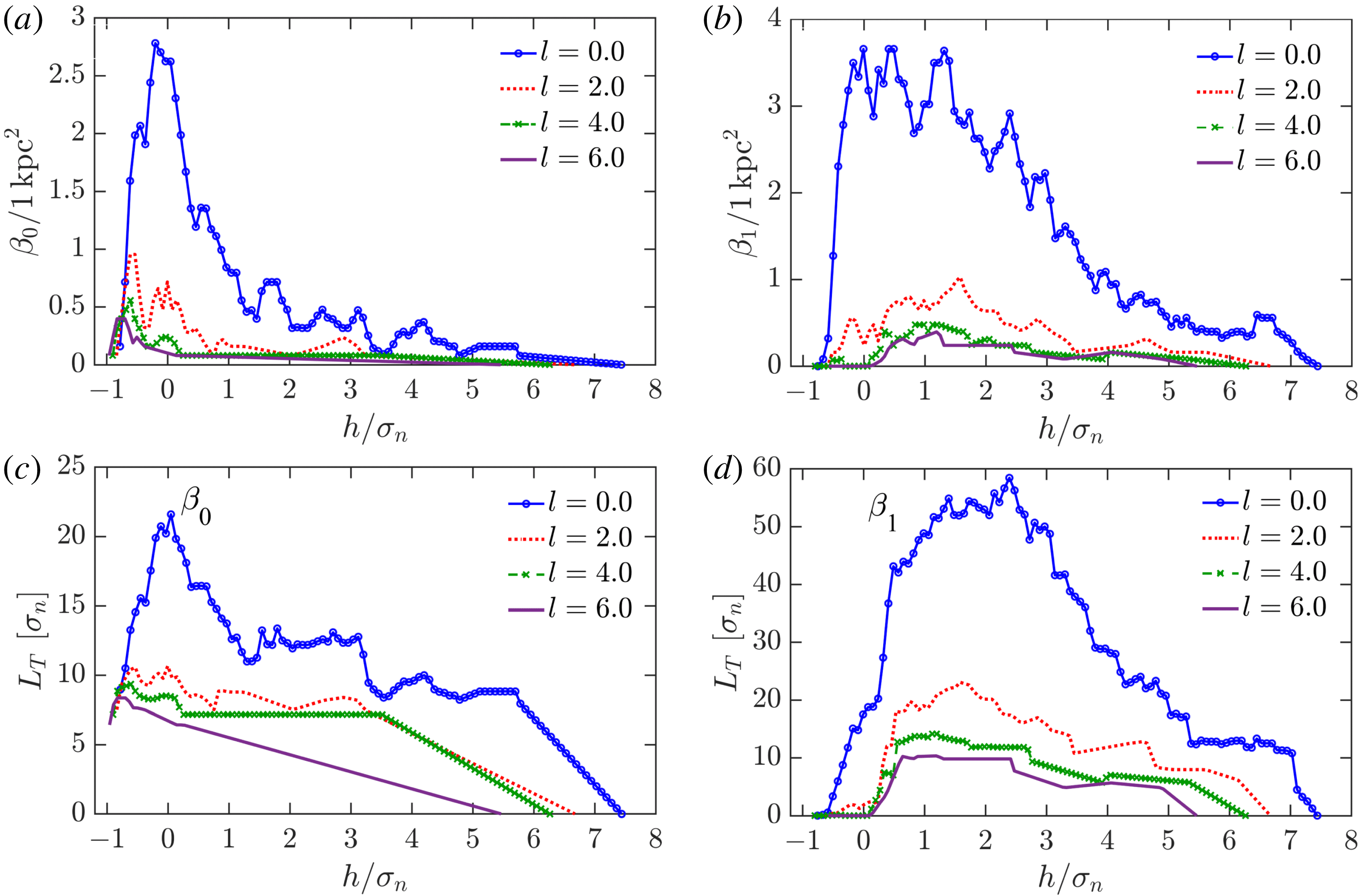
Topological characteristics of the observed H i number density $n$
of figure 10 under Gaussian smoothing. The dependence of the Betti numbers per unit area, (a)
$n$
of figure 10 under Gaussian smoothing. The dependence of the Betti numbers per unit area, (a) $\unicode[STIX]{x1D6FD}_{0}$
and (b)
$\unicode[STIX]{x1D6FD}_{0}$
and (b) $\unicode[STIX]{x1D6FD}_{1}$
versus the isocontour level
$\unicode[STIX]{x1D6FD}_{1}$
versus the isocontour level $h$
(given in the units of
$h$
(given in the units of $\unicode[STIX]{x1D70E}_{n}$
, the standard deviation of
$\unicode[STIX]{x1D70E}_{n}$
, the standard deviation of $n$
). The total length of barcodes (in the units of
$n$
). The total length of barcodes (in the units of $\unicode[STIX]{x1D70E}_{n}$
) is shown as a function of
$\unicode[STIX]{x1D70E}_{n}$
) is shown as a function of $h$
for (c)
$h$
for (c) $\unicode[STIX]{x1D6FD}_{0}$
and (d)
$\unicode[STIX]{x1D6FD}_{0}$
and (d) $\unicode[STIX]{x1D6FD}_{1}$
. Solid blue lines are for the density field at the original resolution, the other lines represent fields smoothed using the Gaussian kernel (5.1) with
$\unicode[STIX]{x1D6FD}_{1}$
. Solid blue lines are for the density field at the original resolution, the other lines represent fields smoothed using the Gaussian kernel (5.1) with $l=2$
, 4 and 6.
$l=2$
, 4 and 6.
As figure 11, but with all curves normalized to unit underlying area.

5 Topological characteristics and the image resolution
In this section we will show that the topological statistics, introduced above, remain stable when the image resolution decreases.
Figure 10(a) shows an original observation of the hydrogen gas density distribution, $n(\unicode[STIX]{x1D719},z)$
, in a region of the Milky Way, from the same data as figure 1(a), after data standardization using (3.1). The image is of 131 pixels height by 349 pixels wide. The horizontal extent of the region shown is about
$n(\unicode[STIX]{x1D719},z)$
, in a region of the Milky Way, from the same data as figure 1(a), after data standardization using (3.1). The image is of 131 pixels height by 349 pixels wide. The horizontal extent of the region shown is about $5.77~\text{kpc}$
, so the pixel width is about
$5.77~\text{kpc}$
, so the pixel width is about $17~\text{pc}$
. The resolution of the data was coarsened by convolving the image with a 2-D Gaussian filter,
$17~\text{pc}$
. The resolution of the data was coarsened by convolving the image with a 2-D Gaussian filter,
 $$\begin{eqnarray}\langle n\rangle (\boldsymbol{x})=\frac{1}{2\unicode[STIX]{x03C0}l^{2}}\int n(\boldsymbol{x}^{\prime })\text{e}^{-(\boldsymbol{x}-\boldsymbol{x}^{\prime })^{2}/(2l^{2})}\,\text{d}^{2}\boldsymbol{x}^{\prime }.\end{eqnarray}$$
We varied the width of the Gaussian kernel as $l=2$
, 4, 6 pixels and the resulting smoothed images are shown in figure 10(b–d). The smoothed images were standardized and a topological filtration applied. Degrading the image resolution using bi-cubic interpolation, where the output pixel value is a weighted average of pixels in the
$l=2$
, 4, 6 pixels and the resulting smoothed images are shown in figure 10(b–d). The smoothed images were standardized and a topological filtration applied. Degrading the image resolution using bi-cubic interpolation, where the output pixel value is a weighted average of pixels in the $4\times 4$
neighbourhood, has the same effect as Gaussian smoothing.
$4\times 4$
neighbourhood, has the same effect as Gaussian smoothing.
The topological filtration of a 2-D image is quantified in terms of two topological variables, the number of components $\unicode[STIX]{x1D6FD}_{0}$
and the number of holes
$\unicode[STIX]{x1D6FD}_{0}$
and the number of holes $\unicode[STIX]{x1D6FD}_{1}$
, both functions of the threshold level
$\unicode[STIX]{x1D6FD}_{1}$
, both functions of the threshold level $h$
. For a statistically stationary random field in two dimensions, the magnitudes of the Betti numbers are proportional to the area of the image and they are therefore usefully presented per unit area. The normalization of the Betti numbers per correlation cell (area or volume) was suggested by Makarenko et al. (Reference Makarenko, Shukurov, Henderson, Rodrigues, Bushby and Fletcher2018) to be more physically informative and sensitive to the topological properties of the random fields rather than its spatial scale. Here we follow the simple approach, calculating the Betti numbers per
$h$
. For a statistically stationary random field in two dimensions, the magnitudes of the Betti numbers are proportional to the area of the image and they are therefore usefully presented per unit area. The normalization of the Betti numbers per correlation cell (area or volume) was suggested by Makarenko et al. (Reference Makarenko, Shukurov, Henderson, Rodrigues, Bushby and Fletcher2018) to be more physically informative and sensitive to the topological properties of the random fields rather than its spatial scale. Here we follow the simple approach, calculating the Betti numbers per $1~\text{kpc}^{2}$
.
$1~\text{kpc}^{2}$
.
The Betti numbers and the total length of the barcodes obtained from filtering the gas density fields of figure 10 are shown in figure 11. It is clear that smoothing with $l=4{-}6$
leads to a significant loss of detail that affects the topological structure of the data, especially for
$l=4{-}6$
leads to a significant loss of detail that affects the topological structure of the data, especially for $\unicode[STIX]{x1D6FD}_{0}$
. It is understandable that smoothing reduces the numbers of both components and holes (i.e.
$\unicode[STIX]{x1D6FD}_{0}$
. It is understandable that smoothing reduces the numbers of both components and holes (i.e. $\unicode[STIX]{x1D6FD}_{0}$
and
$\unicode[STIX]{x1D6FD}_{0}$
and $\unicode[STIX]{x1D6FD}_{1}$
), and contracts the barcodes. However, further normalization of the dependencies
$\unicode[STIX]{x1D6FD}_{1}$
), and contracts the barcodes. However, further normalization of the dependencies $\unicode[STIX]{x1D6FD}_{0}(h)$
,
$\unicode[STIX]{x1D6FD}_{0}(h)$
, $\unicode[STIX]{x1D6FD}_{1}(h)$
and
$\unicode[STIX]{x1D6FD}_{1}(h)$
and $L_{T}(h)$
alleviates the problem of image resolution. Figure 12 presents the same results as figure 11 but normalized to unit area under each curve. Thus, images of different resolutions can be compared directly provided both the observable quantities and the results of their topological filtration have been properly standardized.
$L_{T}(h)$
alleviates the problem of image resolution. Figure 12 presents the same results as figure 11 but normalized to unit area under each curve. Thus, images of different resolutions can be compared directly provided both the observable quantities and the results of their topological filtration have been properly standardized.
Thus, topological filtration helps to identify a range of resolutions where statistical properties of the random field remain stable, extending this beyond second-order moments or power spectra. For the specific field of the interstellar gas number density, smoothing affects $\unicode[STIX]{x1D6FD}_{0}$
more than
$\unicode[STIX]{x1D6FD}_{0}$
more than $\unicode[STIX]{x1D6FD}_{1}$
. For example,
$\unicode[STIX]{x1D6FD}_{1}$
. For example, $\unicode[STIX]{x1D6FD}_{1}(h)$
still contains some details for
$\unicode[STIX]{x1D6FD}_{1}(h)$
still contains some details for $l=4$
whereas
$l=4$
whereas $\unicode[STIX]{x1D6FD}_{0}(h)$
loses them for
$\unicode[STIX]{x1D6FD}_{0}(h)$
loses them for $h\gtrsim 0.5\unicode[STIX]{x1D70E}_{n}$
. This suggests that
$h\gtrsim 0.5\unicode[STIX]{x1D70E}_{n}$
. This suggests that $n(\boldsymbol{x})$
has narrow minima and broad maxima, so that the minima are lost first as the resolution is being reduced.
$n(\boldsymbol{x})$
has narrow minima and broad maxima, so that the minima are lost first as the resolution is being reduced.
6 Comparing the observed and simulated gas density fields
The H i number density $n\;(\text{atom}~\text{cm}^{-3})$
from the GASS survey (Kalberla et al.
Reference Kalberla2010) in
$n\;(\text{atom}~\text{cm}^{-3})$
from the GASS survey (Kalberla et al.
Reference Kalberla2010) in $5~\text{kpc}$
-wide strips along the galactic mid-plane (
$5~\text{kpc}$
-wide strips along the galactic mid-plane ( $|z|\leqslant 2.5~\text{kpc}$
) at
$|z|\leqslant 2.5~\text{kpc}$
) at $R=10~\text{kpc}$
(a) and
$R=10~\text{kpc}$
(a) and $20~\text{kpc}$
(b). The vertical lines in (a) separate three regions where gas density apparently has distinct properties and which are analysed separately.
$20~\text{kpc}$
(b). The vertical lines in (a) separate three regions where gas density apparently has distinct properties and which are analysed separately.

Results of topological analysis of the H i number density in four regions in the Milky Way (as specified in the legends) shown in figure 13 and described in the text. (a,b) Betti numbers per unit area, $\unicode[STIX]{x1D6FD}_{0}$
and
$\unicode[STIX]{x1D6FD}_{0}$
and $\unicode[STIX]{x1D6FD}_{1}$
, respectively. (c,d) Total barcode lengths for
$\unicode[STIX]{x1D6FD}_{1}$
, respectively. (c,d) Total barcode lengths for $\unicode[STIX]{x1D6FD}_{0}$ $\unicode[STIX]{x1D6FD}_{1}$
, respectively. All variables are presented as functions of the level height
$\unicode[STIX]{x1D6FD}_{1}$
, respectively. All variables are presented as functions of the level height $h$
in the units of the standard deviation of the density variations
$h$
in the units of the standard deviation of the density variations $\unicode[STIX]{x1D70E}_{n}$
. All curves are normalized to the unit underlying area.
$\unicode[STIX]{x1D70E}_{n}$
. All curves are normalized to the unit underlying area.

As figure 14 but for the simulated interstellar gas. The error bars represent the standard deviation of the scatter of the corresponding variable between the twelve snapshots used for the analysis.
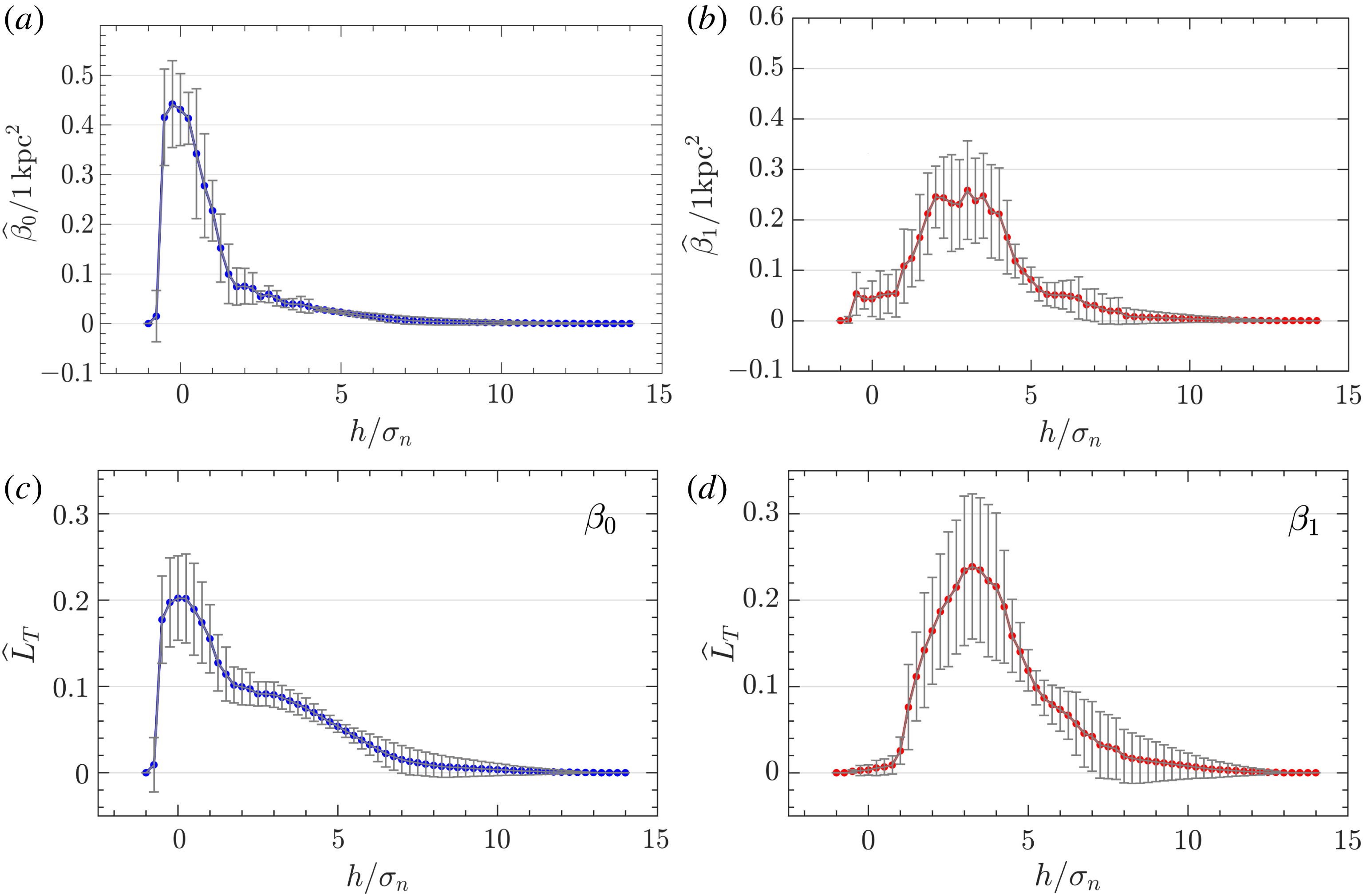
In this section we compare 2-D gas density fields observed in different parts of the Milky Way (from the GASS survey – Kalberla et al. Reference Kalberla2010) and taken from 3-D MHD simulations of the ISM (Gent et al. Reference Gent, Shukurov, Fletcher, Sarson and Mantere2013a ,Reference Gent, Shukurov, Sarson, Fletcher and Mantere b ).
The GASS data, shown in figure 13, are from cylindrical surfaces at $R=10$
and
$R=10$
and $20~\text{kpc}$
. We consider separately three regions at
$20~\text{kpc}$
. We consider separately three regions at $R=10~\text{kpc}$
, separated by the vertical lines, that have equal areas. The average values of
$R=10~\text{kpc}$
, separated by the vertical lines, that have equal areas. The average values of $n$
are quite different in the three regions because of the spiral arm pattern of a significant strength at
$n$
are quite different in the three regions because of the spiral arm pattern of a significant strength at $R=10~\text{kpc}$
. Its strength decreases with
$R=10~\text{kpc}$
. Its strength decreases with $R$
and variations of
$R$
and variations of $n$
with azimuth
$n$
with azimuth $\unicode[STIX]{x1D719}$
are much weaker at
$\unicode[STIX]{x1D719}$
are much weaker at $R=20~\text{kpc}$
(note the difference in the colour schemes in the two panels of figure 13). Therefore, we do not divide the region at
$R=20~\text{kpc}$
(note the difference in the colour schemes in the two panels of figure 13). Therefore, we do not divide the region at $R=20~\text{kpc}$
into separate parts.
$R=20~\text{kpc}$
into separate parts.
We also analysed, using the same tools as for the observed gas distribution, gas density obtained from numerical simulations of the interstellar medium in a $1~\text{kpc}\times 1~\text{kpc}\times 2~\text{kpc}$
domain. Parameters of the simulation are close to those in the Solar neighbourhood,
$1~\text{kpc}\times 1~\text{kpc}\times 2~\text{kpc}$
domain. Parameters of the simulation are close to those in the Solar neighbourhood, $R=8.5~\text{kpc}$
. Random flows in the simulated ISM are driven by explosions of supernova stars that inject into the system large amounts of thermal and kinetic energy. The model includes, among other effects, large-scale velocity shear due to the galactic differential rotation, stratification in a gravitational field of stars, heating by the supernovae, optically thin radiative cooling and magnetic fields which are due to a mean-field dynamo action. We took a vertical cross-section through the middle of the computational domain at 12 moments separated by
$R=8.5~\text{kpc}$
. Random flows in the simulated ISM are driven by explosions of supernova stars that inject into the system large amounts of thermal and kinetic energy. The model includes, among other effects, large-scale velocity shear due to the galactic differential rotation, stratification in a gravitational field of stars, heating by the supernovae, optically thin radiative cooling and magnetic fields which are due to a mean-field dynamo action. We took a vertical cross-section through the middle of the computational domain at 12 moments separated by $2.5\unicode[STIX]{x1D70F}$
where
$2.5\unicode[STIX]{x1D70F}$
where $\unicode[STIX]{x1D70F}$
is the correlation length of the random flow in the time domain. The time lag is large enough for the snapshots to be statistically independent to a reasonable approximation. Figure 1(b) shows one such cross-section.
$\unicode[STIX]{x1D70F}$
is the correlation length of the random flow in the time domain. The time lag is large enough for the snapshots to be statistically independent to a reasonable approximation. Figure 1(b) shows one such cross-section.
We standardized the data using (3.1), applied the topological filtration described in § 2 and computed the Betti numbers and barcode lengths for each level $h$
. The results were normalized to eliminate, as much as possible, the effects of the image resolution and systematic trends as described in §§ 4 and 5. The observations at
$h$
. The results were normalized to eliminate, as much as possible, the effects of the image resolution and systematic trends as described in §§ 4 and 5. The observations at $R=20~\text{kpc}$
have a lower linear resolution than at
$R=20~\text{kpc}$
have a lower linear resolution than at $R=10~\text{kpc}$
because the angular width of the telescope beam was the same. Moreover, the resolution in each panel of figure 13 decreases from right to left, since the right end of the galactocentric azimuthal range shown is much closer to the Sun. The numerical simulations have a resolution higher than any of the observational data.
$R=10~\text{kpc}$
because the angular width of the telescope beam was the same. Moreover, the resolution in each panel of figure 13 decreases from right to left, since the right end of the galactocentric azimuthal range shown is much closer to the Sun. The numerical simulations have a resolution higher than any of the observational data.
The results shown in figure 14 suggest that the gas distributions in the right-hand part of figure 13(a) and in figure 13(b) are topologically similar, and both are different from the other two regions at $R=10~\text{kpc}$
. This can be explained by the fact that the left and middle zones in figure 13 mostly lie within the Carina spiral arm (roughly, the azimuthal range
$R=10~\text{kpc}$
. This can be explained by the fact that the left and middle zones in figure 13 mostly lie within the Carina spiral arm (roughly, the azimuthal range $300^{\circ }<\unicode[STIX]{x1D719}<250^{\circ }$
) whereas the right zone mostly comprises the inter-arm region close to the Sun (roughly, the azimuthal range
$300^{\circ }<\unicode[STIX]{x1D719}<250^{\circ }$
) whereas the right zone mostly comprises the inter-arm region close to the Sun (roughly, the azimuthal range $230^{\circ }<\unicode[STIX]{x1D719}<200^{\circ }$
). Spiral arms are the sites of higher star formation rate. Star formation is very likely to produce a more energetic forcing of the interstellar turbulence, via supernova explosions and expanding supernova remnants as well as winds from massive stars. The outer Galaxy
$230^{\circ }<\unicode[STIX]{x1D719}<200^{\circ }$
). Spiral arms are the sites of higher star formation rate. Star formation is very likely to produce a more energetic forcing of the interstellar turbulence, via supernova explosions and expanding supernova remnants as well as winds from massive stars. The outer Galaxy $R\gtrsim 16~\text{kpc}$
hosts only weak star formation and spiral arms are expected to be less pronounced there; condition of the interstellar gas may be expected to be similar to that in the inter-arm regions near the Sun. Different properties of turbulence in the arms and inter-arm regions are often suspected but there is little observational support for this assumption, mainly because the difference is rather subtle. It is remarkable that the topological data analysis appears to be more sensitive to the expected difference than other methods, but this suggestion needs to be carefully verified.
$R\gtrsim 16~\text{kpc}$
hosts only weak star formation and spiral arms are expected to be less pronounced there; condition of the interstellar gas may be expected to be similar to that in the inter-arm regions near the Sun. Different properties of turbulence in the arms and inter-arm regions are often suspected but there is little observational support for this assumption, mainly because the difference is rather subtle. It is remarkable that the topological data analysis appears to be more sensitive to the expected difference than other methods, but this suggestion needs to be carefully verified.
We show in figure 15 the result of a topological filtration of the simulated gas density. The curves represent means and the error bars the standard deviations across the twelve snapshots. The pronounced, rather symmetric maximum of $\unicode[STIX]{x1D6FD}_{1}(h)$
appears to be closest to that for the middle zone of the observational data at
$\unicode[STIX]{x1D6FD}_{1}(h)$
appears to be closest to that for the middle zone of the observational data at $R=10~\text{kpc}$
(the dotted red lines in figure 14). That region in the observations shows highly skewed, long-tailed dependence on
$R=10~\text{kpc}$
(the dotted red lines in figure 14). That region in the observations shows highly skewed, long-tailed dependence on $h$
for
$h$
for $\unicode[STIX]{x1D6FD}_{0}$
, which is also the case for the simulated data. The middle zone of figure 13 is dominated by the Carina spiral arm, and this suggests that the parameters selected for the numerical simulation are more appropriate for the spiral arms of the Milky Way. The promise of topological data analysis is quite evident but more work with both observational and numerical data are required to verify and substantiate these suggestions.
$\unicode[STIX]{x1D6FD}_{0}$
, which is also the case for the simulated data. The middle zone of figure 13 is dominated by the Carina spiral arm, and this suggests that the parameters selected for the numerical simulation are more appropriate for the spiral arms of the Milky Way. The promise of topological data analysis is quite evident but more work with both observational and numerical data are required to verify and substantiate these suggestions.
7 Conclusions and discussion
We have outlined an approach to topological data analysis that allows for comparisons of random fluctuations in different data sets that does not rely on assumptions of Gaussian statistics. The analysis follows the following steps:
(i) Standardize the data by subtracting the mean and normalizing by the standard deviation. This makes the topological measures insensitive to the magnitude of the data.
(ii) Compute the Betti numbers $\unicode[STIX]{x1D6FD}_{0}$
and
$\unicode[STIX]{x1D6FD}_{1}$
(for two-dimensional data), and the total barcode length, at each level
$h$
of a topological filtration.
$\unicode[STIX]{x1D6FD}_{0}$
and
$\unicode[STIX]{x1D6FD}_{1}$
(for two-dimensional data), and the total barcode length, at each level
$h$
of a topological filtration.(iii) Normalize the Betti numbers and barcode lengths to the unit length or area as appropriate.
(iv) Normalize the results further to unit area under each curve.


Working with the normalized curves removes the sensitivity of the topological measures to the presence of large-scale trends and to the resolution of the data. Topologically similar data will have similar normalized variations of $\unicode[STIX]{x1D6FD}_{0}$
,
$\unicode[STIX]{x1D6FD}_{0}$
, $\unicode[STIX]{x1D6FD}_{1}$
and
$\unicode[STIX]{x1D6FD}_{1}$
and $L_{T}$
with
$L_{T}$
with $h$
.
$h$
.
The effects of the standardization and systematic trends depend on the scale separation between the mean values and fluctuations. For example, for a weaker scale (or frequency) separation between the two terms in (3.2), the points in the standardized persistence diagram similar to figure 5(c) no longer coincide. For $f(x)$
of this form, the standardization is still useful, when the frequency of the second term is changed from 0.2 to 0.5, but not for frequency ratios that are still closer to unity. The marginal frequency ratio (or scale separation) is, of course, model dependent.
$f(x)$
of this form, the standardization is still useful, when the frequency of the second term is changed from 0.2 to 0.5, but not for frequency ratios that are still closer to unity. The marginal frequency ratio (or scale separation) is, of course, model dependent.
By applying this approach to observations and numerical simulations of the gas density distribution in the turbulent interstellar gas of the Milky Way, we were able to distinguish observations of the spiral arms from those of inter-arm regions and to identify which regions of the Galaxy most closely resemble the domain of the simulations.
The kinetic and magnetic Reynolds numbers of the simulations used here do not exceed 100 (Hollins et al. Reference Hollins, Sarson, Shukurov, Fletcher and Gent2017) and are by far smaller than those in the interstellar gas of the Milky Way. This means that the simulated fluctuations have a much narrower range of scales than the observational data. However, comparison of figures 14 and 15 suggests that this does not undermine the topological comparison and its discriminatory power. This is understandable since the whole approach of topological filtration isolates the most significant, ‘persistent’ features of random fields, and these are dominated by fluctuations of larger scales. Robustness of the topological filtration under changing image resolution has a similar reason.
Acknowledgements
We gratefully acknowledge financial support of the Leverhulme Trust (Research grant RPG-2014-427) and Institute of Information and Computational Technologies (grant AR05134227).



