


1. Introduction
The presence of a bluff body in a shear flow imposes an adverse pressure gradient on the approaching fluid, potentially leading to upstream separation and the formation of necklace (horseshoe) vortices that wrap around the body. Owing to their fundamental and practical significance, such vortex systems have been extensively studied in wall-bounded boundary-layer junction flows (Baker Reference Baker1978; Simpson Reference Simpson2001; Elahi, Lange & Lynch Reference Elahi, Lange and Lynch2019). In contrast, study of the interaction between a laminar free-shear flow and a bluff body has received much less attention, despite the potential of its study to reveal a more comprehensive understanding of three-dimensional (3-D) vortical flow, unsteady separation and vortex formation.
Comparison of (a) boundary-layer junction flow and (b) laminar shear-wake–cylinder interaction (this study). Note that the top panel in (b) presents a laminar shear-wake in its general form, whereas the bottom panel shows a laminar wake. In junction flow, the cylinder imposes an adverse pressure gradient on a wall-bounded boundary layer, leading to a surface flux of vorticity and separation at the wall, and vortex roll-up. In contrast, in the shear-wake interaction, no rigid wall separates the two streams. Opposite-signed vorticity resides in adjacent shear layers generated upstream at the splitter plate. Separation between the streams, if present, develops upstream of the cylinder along a deformable dividing stream surface rather than at a solid boundary. Therefore, since there is no wall, there is no vorticity flux.

While shear-wake–cylinder interaction shares certain features with the boundary-layer junction flow, the underlying physics differ fundamentally. In particular, no rigid wall exists to provide a site for vorticity flux into the flow. The laminar shear-wakes considered herein consist of adjacent shear layers with opposite-signed vorticity, and the present study examines how such a configuration responds to the adverse pressure gradient imposed by a cylinder. To properly frame this problem, we first review vortex formation in wall-bounded junction flows, followed by a brief discussion of separation and vorticity generation before introducing the key features of shear-wake–cylinder interaction. Figure 1 provides a comparison between the two flow configurations.
1.1. Wall-bounded vortex-system formation
The impact of an adverse pressure gradient on a boundary layer is well documented, e.g. Gaster (Reference Gaster1969) and Pauley, Moin & Reynolds (Reference Pauley, Moin and Reynolds1990). An adverse pressure gradient can lead to separation of the boundary layer if the pressure gradient is of sufficient magnitude or duration. One specific scenario arises when a bluff body, such as a cylinder, imposes a streamwise adverse pressure gradient on a laminar boundary layer as schematically depicted in figure 1(a). In such a junction flow, 3-D flow separation and downstream evolution of the vortices occur largely owing to the momentum deficit and surface vorticity flux induced by the cylinder-imposed adverse pressure gradient. Accordingly, the rolled-up vortices reorient due to the interaction between 3-D pressure gradients coupled with a dominant flux of streamwise momentum. Collectively, these processes lead to the formation of a system of necklace vortices, commonly known as horseshoe vortices, as discussed in detail by e.g. Simpson (Reference Simpson2001).
Baker (Reference Baker1978) was among the first to experimentally investigate the formation and topology of laminar junction-flow vortex systems around a circular cylinder, largely using smoke-flow visualisation in a wind tunnel. He identified the key parameters governing the vortex system and expressed them in non-dimensional form as
 \begin{align} \frac {x_v}{d}, \frac {x_s}{d}, \frac {\textit{fd}}{U} = \chi \!\left (\frac {\textit{Ud}}{\nu }, \frac {d}{\delta ^*}\right )\!, \end{align}
where $x_v$
and
$x_v$
and $x_s$
denote the locations of the vortex centre and separation line, respectively,
$x_s$
denote the locations of the vortex centre and separation line, respectively, $d$
is the cylinder diameter,
$d$
is the cylinder diameter, $U$
is the free-stream velocity,
$U$
is the free-stream velocity, $\nu$
is the kinematic viscosity and
$\nu$
is the kinematic viscosity and $\delta ^*$
is the boundary-layer displacement thickness at the cylinder location in the absence of the cylinder. Here, the variable
$\delta ^*$
is the boundary-layer displacement thickness at the cylinder location in the absence of the cylinder. Here, the variable $f$
denotes the oscillation frequency of vortices and
$f$
denotes the oscillation frequency of vortices and $ \textit{fd}/U$
is the Strouhal number
$ \textit{fd}/U$
is the Strouhal number $(\textit{St})$
. The non-dimensional parameter
$(\textit{St})$
. The non-dimensional parameter $ \textit{Ud}/\nu$
is the Reynolds number
$ \textit{Ud}/\nu$
is the Reynolds number $(Re)$
, and
$(Re)$
, and $d/\delta ^*$
is the ratio of cylinder diameter to boundary-layer displacement thickness.
$d/\delta ^*$
is the ratio of cylinder diameter to boundary-layer displacement thickness.
Baker (Reference Baker1979) subsequently documented multiple laminar vortex-system configurations (summarised in figure 2). With increasing $ \textit{Re}$
, the number of vortices increased from two to four and then to six before the regime became unstable. He also related the onset of unsteadiness to the upstream pressure distribution: steady regimes exhibited local pressure minima associated with vortex cores, whereas unsteady regimes showed a monotonic pressure rise towards the cylinder.
$ \textit{Re}$
, the number of vortices increased from two to four and then to six before the regime became unstable. He also related the onset of unsteadiness to the upstream pressure distribution: steady regimes exhibited local pressure minima associated with vortex cores, whereas unsteady regimes showed a monotonic pressure rise towards the cylinder.
Visbal (Reference Visbal1989, Reference Visbal1991a
,
Reference Visbalb
) conducted numerical simulations of a similar junction flow and largely confirmed Baker’s observed regimes. Visbal further noted that the distinction between steady and unsteady regimes is reflected not only in pressure distributions but also in surface quantities such as skin friction, which were not available in Baker (Reference Baker1979) owing to experimental limitations. In addition, Baker identified a narrow range of Reynolds numbers in which the vortices oscillated between modes before transition; Visbal (Reference Visbal1989) termed this behaviour ‘rocking motion’ and noted that it did not appear in his simulations, likely due to limited ability to finely adjust $ \textit{Re}$
a priori.
$ \textit{Re}$
a priori.
In both experimental and numerical studies, a thin splitter plate attached to the cylinder rear was used to suppress Kármán vortex shedding and isolate the intrinsic unsteadiness of the junction-flow vortex system. For further details on laminar and turbulent junction-flow vortex systems, the reader is referred to the review by Simpson (Reference Simpson2001).
Number of vortices in laminar boundary-layer/cylinder junction flow. Here, $d/\delta ^*$
represents the ratio of the cylinder diameter to the boundary-layer displacement thickness and
$d/\delta ^*$
represents the ratio of the cylinder diameter to the boundary-layer displacement thickness and $ \textit{Ud}/\nu$
is the Reynolds number
$ \textit{Ud}/\nu$
is the Reynolds number $(Re)$
defined based on the cylinder diameter. Data are replotted from Baker (Reference Baker1979).
$(Re)$
defined based on the cylinder diameter. Data are replotted from Baker (Reference Baker1979).

1.2. Separation and vorticity generation
The generation of vortical structures in two-dimensional (2-D) steady wall flows is contingent upon separation, which requires the nullification of velocity and its derivative (skin friction) at the wall. These conditions are both necessary and sufficient for separation, known as the Prandtl criteria (see, e.g. Haller Reference Haller2004). In this classical framework, separation manifests as a change in flow topology, where a distinguished separatrix streamline, emanating from a singular separation point, divides the flow. Because the separation location remains fixed in space, 2-D steady separation admits a purely Eulerian formulation. Upon separation, the detached shear layer typically rolls up into identifiable vortical structures.
The extension to unsteady flows builds upon steady flow over moving walls and led to the Moore–Rott–Sears criterion (Sears & Telionis Reference Sears and Telionis1975), which remains fundamentally Eulerian. In this formulation, separation corresponds to a zero-velocity and zero-vorticity point in a suitably advecting reference frame, while the wall shear does not necessarily vanish instantaneously. Thus, unlike steady separation, unsteady separation cannot be characterised solely by vanishing skin friction.
When it comes to 3-D separation, the most common prescription is based on observations of skin-friction lines (Sherman Reference Sherman1990). These lines, analogous to streamlines, do not intersect except at specific points where the shear stress $(\tau )$
vanishes, rendering the vectors indeterminate. The significance of this criterion, albeit Eulerian, is underscored in the literature on 2-D steady and unsteady flow separation, as highlighted by Sherman (Reference Sherman1990), who referenced the earlier work of Lighthill (Reference Lighthill1963) and emphasised skin friction as an index of separation.
$(\tau )$
vanishes, rendering the vectors indeterminate. The significance of this criterion, albeit Eulerian, is underscored in the literature on 2-D steady and unsteady flow separation, as highlighted by Sherman (Reference Sherman1990), who referenced the earlier work of Lighthill (Reference Lighthill1963) and emphasised skin friction as an index of separation.
Haller (Reference Haller2004) reformulated 2-D unsteady separation within a Lagrangian dynamical-systems framework, identifying separating profiles with unstable manifolds of boundary trajectories under asymptotic hyperbolicity. In this view, separation is a material instability governed by invariant manifolds rather than instantaneous streamline topology. Subsequent developments extended invariant-manifold theory to 3-D and slip-boundary configurations using normally hyperbolic invariant manifolds (NHIMs) (Surana, Grunberg & Haller Reference Surana, Grunberg and Haller2006; Lekien & Haller Reference Lekien and Haller2008), introducing dividing stream surfaces as 3-D analogues of 2-D separatrices. These frameworks, however, rely on exponential hyperbolicity and on the presence of material transport barriers that are non-penetrable in the normal direction.
More recent work has demonstrated that separation can occur even in the absence of identifiable saddles or invariant manifolds. In slow–fast, non-hyperbolic regimes, Surana & Haller (Reference Surana and Haller2008) introduced ghost manifolds: finite-time material structures that transiently organise spike-like ejection despite the absence of classical hyperbolicity. Finite-time transport analysis further revealed that instantaneous Eulerian saddles need not correspond to true separation, whereas Lagrangian coherent structures (LCS), identified via finite-time Lyapunov exponents (FTLE), can reveal off-wall transport barriers (Surana et al. Reference Surana, Jacobs, Grunberg and Haller2008; Miron et al. Reference Miron, Vétel, Garon and Haller2015). Most recently, separation onset has been given an exact finite-time Lagrangian definition based on curvature-driven material spike formation (Serra & Haller Reference Serra and Haller2018; Santhosh & Haller Reference Santhosh and Haller2023), demonstrating that detachment is fundamentally a short-time folding instability of material lines or surfaces, applicable to unsteady flows with fixed or moving boundaries and capable of explaining both wall-attached and apparently off-wall separation.
These developments highlight that modern separation theory increasingly emphasises finite-time material deformation rather than wall-based singularities. However, the majority of existing formulations, whether invariant-manifold-based, NHIM-based or slip-boundary-based, presume the existence of a material barrier that is kinematically non-penetrable (i.e. a physical wall). In contrast, in the present shear-wake configuration, the interface between the two streams is a deformable dividing stream surface across which opposite-signed vorticity may diffuse and partially annihilate (see figure 1 b). This surface therefore does not strictly satisfy the impermeability assumptions inherent to classical slip-wall or normally hyperbolic frameworks. As such, separation in this configuration cannot be interpreted as detachment from a rigid or idealised slip boundary, but rather emerges from the finite-time interaction and reorganisation of two adjacent vortical streams in the absence of a solid wall.
The generation of vorticity in constant-density isothermal flows occurs through tangential acceleration of the flow at a surface, as described in detail by Morton (Reference Morton1984). This acceleration can stem from either a tangential pressure gradient or a tangential acceleration at the boundary. In scenarios involving rapid vorticity generation, the resulting distribution of the generated vorticity occurs primarily through diffusion and minimally through advection. Alternatively, although not applicable to this study, in cases where vorticity is generated at a slower pace, the processes of vorticity generation and distribution become intricately intertwined due to the gradual nature of vorticity generation and the potential role of viscosity in the process.
For the boundary-layer junction-flow scenario, the vorticity in the approaching flat plate boundary layer is generated when the free-stream non-vortical flow encounters the leading edge of the plate. This vorticity then diffuses as it is carried downstream within the boundary layer until it reaches the cylinder. Here, flow blockage imposes an adverse pressure gradient on the vortical flow, causing it to decelerate, and eventually results in flow separation. In this case, a surface flux of vorticity is central to the separation process. Assuming a 2-D boundary layer before any separation occurs near the cylinder, we consider the Prandtl boundary-layer equation for steady flow
 \begin{align} u\frac {\partial u}{\partial x}+ v\frac {\partial u}{\partial y} = -\frac {1}{\rho }\frac {{\rm d}p}{{\rm d}x}+\nu \frac {\partial ^2u}{\partial y^2} = -\frac {1}{\rho }\frac {{\rm d}p}{{\rm d}x}+\nu \frac {\partial ( -\omega _z)}{\partial y}. \end{align}
The last term on the right-hand side of (1.2) holds in general owing to the fact that $\partial v/\partial x$
is subdominant under the boundary-layer approximation and more specifically equals zero at
$\partial v/\partial x$
is subdominant under the boundary-layer approximation and more specifically equals zero at $y = 0$
(
$y = 0$
( $\omega _z = \partial v/\partial x - \partial u/\partial y$
). With regard to (1.2), we focus our attention on the streamwise–wall-normal plane passing through the cylinder centre (see figure 1
a). At the wall, all terms on the left-hand side vanish, leading to the balance between the pressure gradient and the flux of vorticity upstream of the separation point. This yields
$\omega _z = \partial v/\partial x - \partial u/\partial y$
). With regard to (1.2), we focus our attention on the streamwise–wall-normal plane passing through the cylinder centre (see figure 1
a). At the wall, all terms on the left-hand side vanish, leading to the balance between the pressure gradient and the flux of vorticity upstream of the separation point. This yields
 \begin{align} \frac {1}{\rho }\frac {{\rm d}p}{{\rm d}x} = -\nu \frac {\partial (\omega _z)}{\partial y}. \end{align}
A schematic of the interplay between the adverse pressure gradient and the attendant flux of vorticity is depicted in figure 1(a). Physically, (1.3) reveals that the adverse streamwise pressure gradient results in a counterbalancing flux of vorticity in the cross-stream direction that is generated along the flat wall. This flux of $\omega _z$
is of a sign opposite to that in the approaching boundary layer, and thus the viscous diffusion of opposing-signed
$\omega _z$
is of a sign opposite to that in the approaching boundary layer, and thus the viscous diffusion of opposing-signed $\omega _z$
eventually annihilates the boundary-layer vorticity until steady separation is attained, e.g. Lighthill (Reference Lighthill1963).
$\omega _z$
eventually annihilates the boundary-layer vorticity until steady separation is attained, e.g. Lighthill (Reference Lighthill1963).
1.3. Laminar shear-wake interaction with circular cylinder
As discussed earlier, in contrast to wall-bounded junction flow (figure 1
a), the present study concerns the interaction of a two-stream, laminar, free-shear flow with a circular cylinder (see figure 1
b). We first consider a symmetric laminar wake generated by two streams of equal speed confluent at the trailing edge of a splitter plate (see figure 1
a and its mirror in the $x$
–
$x$
– $z$
plane to generate the bottom panel in figure 1
b). At the splitter plate trailing edge, the symmetric wake comprises two mirror-image boundary layers whose vorticity distributions interact and mutually annihilate along the
$z$
plane to generate the bottom panel in figure 1
b). At the splitter plate trailing edge, the symmetric wake comprises two mirror-image boundary layers whose vorticity distributions interact and mutually annihilate along the $x$
-axis. In the more general case, unequal stream velocities generate a laminar shear-wake (see figure 1
b top panel). Following annihilation of the weaker-signed vorticity, the shear-wake evolves into a two-stream mixing layer with a single dominant sign of vorticity and a velocity profile approximated by a hyperbolic tangent distribution (e.g. Koochesfahani & Frieler Reference Koochesfahani and Frieler1989). The introduction of a cylinder interrupts this evolution and promotes vortex roll-up and possible flow separation through mechanisms that differ fundamentally from classical wall-based separation (see figure 6
a).
$x$
-axis. In the more general case, unequal stream velocities generate a laminar shear-wake (see figure 1
b top panel). Following annihilation of the weaker-signed vorticity, the shear-wake evolves into a two-stream mixing layer with a single dominant sign of vorticity and a velocity profile approximated by a hyperbolic tangent distribution (e.g. Koochesfahani & Frieler Reference Koochesfahani and Frieler1989). The introduction of a cylinder interrupts this evolution and promotes vortex roll-up and possible flow separation through mechanisms that differ fundamentally from classical wall-based separation (see figure 6
a).
Similar to boundary-layer junction flow, the vorticity in each stream of a shear-wake is generated far upstream of the cylinder. When the cylinder interrupts the laminar shear-wake, the streams become susceptible to separation. During separation, the vorticity rolls up while the total vorticity is approximately conserved and transported downstream as vortex tubes. This process involves vorticity reorientation due to the interaction of the 3-D pressure and velocity fields around the cylinder with the free-stream momentum. In both configurations, vorticity annihilation occurs only through viscous diffusion under isothermal, constant-density conditions.
Unlike junction flow, no physical wall separates the two shear-wake streams containing adjacent regions of opposite-signed vorticity. Consequently, the no-slip and no-penetration constraints and the associated pressure-gradient-induced vorticity flux from a wall are absent. The two streams therefore interact more freely and may be conceptualised as being separated by a deformable dividing stream surface acting as a slip interface. In this configuration, the interpretation based on (1.2) and (1.3) no longer applies, since the left-hand side of (1.2) is not zero along the hypothesised dividing surface. Any separation therefore occurs away from the cylinder and may be stationary or unsteady depending on the flow conditions. This will be discussed further when the vortex regimes are introduced.
The interaction of a wake with a bluff body and the potential formation of horseshoe or necklace vortices were first investigated by Nagib & Hodson (Reference Nagib and Hodson1977), who reported a nonlinear dependence of vortex formation on wake vorticity content and velocity defect. They observed that increasing free-stream velocity promotes vortex formation, while increasing the separation distance between the wake generator and the cylinder attenuates vortex strength. The most comprehensive prior study of shear-wake–cylinder interaction is that of Lee (Reference Lee1994), who identified necklace vortices and documented multiple steady and unsteady regimes, including a no-vortex regime at low Reynolds numbers.
Within the broader context of flow separation and vortex formation, the laminar shear-wake–cylinder interaction offers a unique opportunity to examine steady and unsteady separation in a wall-free environment. Despite substantial theoretical advances in separation theory, the present configuration suggests that separation in such flows remains an unsettled phenomenon requiring further scrutiny. The current investigation seeks to address this gap by: $(i)$
mapping vortex regimes across Reynolds number and shear ratio (defined in § 3),
$(i)$
mapping vortex regimes across Reynolds number and shear ratio (defined in § 3), $(\textit{ii})$
documenting the key mechanisms governing vortex formation through detailed flow visualisation and
$(\textit{ii})$
documenting the key mechanisms governing vortex formation through detailed flow visualisation and $(\textit{iii})$
proposing a mechanistic interpretation of the vortex systems observed.
$(\textit{iii})$
proposing a mechanistic interpretation of the vortex systems observed.
Accordingly, the conceptual distinctions outlined above are not merely historical. They are necessary to properly interpret separation in the present wall-free configuration, where classical wall-based criteria are inapplicable and separation must be understood in terms of finite-time material reorganisation of interacting shear layers.
2. Experimental facility and flow visualisation technique
2.1. Experimental facility
The experiments were conducted in a closed-loop water-channel facility at the University of Melbourne. The channel is equipped with two matched pumps that are individually controlled by variable-frequency drives, enabling a range of flow velocities from $0.025\,\mathrm{}$
to
$0.025\,\mathrm{}$
to $0.5\,\mathrm{m\, s^{-1}}$
. The
$0.5\,\mathrm{m\, s^{-1}}$
. The $0.6\,\mathrm{m}$
-long test section cross-sectional dimensions of
$0.6\,\mathrm{m}$
-long test section cross-sectional dimensions of $ 0.154 \times 0.154\,\mathrm{m^2}$
and is evenly divided by a splitter plate that ends near the inlet of the test section. The test section has optical access at the bottom, side and end views. A cylinder,
$ 0.154 \times 0.154\,\mathrm{m^2}$
and is evenly divided by a splitter plate that ends near the inlet of the test section. The test section has optical access at the bottom, side and end views. A cylinder, $0.152\,\mathrm{m}$
in length and
$0.152\,\mathrm{m}$
in length and $0.0254\,\mathrm{m}$
in diameter, fabricated from black polyoxymethylene (Delrin) was mounted downstream of the splitter plate. The cylinder was positioned at a depth that corresponds to half the total depth of water (
$0.0254\,\mathrm{m}$
in diameter, fabricated from black polyoxymethylene (Delrin) was mounted downstream of the splitter plate. The cylinder was positioned at a depth that corresponds to half the total depth of water ( $15.4\,\mathrm{cm}$
) within the test section and
$15.4\,\mathrm{cm}$
) within the test section and $5-10\,\mathrm{cm}$
downstream of the splitter plate. In order to increase the viscosity of water and improve the precision in attaining a given Reynolds number, a solution comprising approximately
$5-10\,\mathrm{cm}$
downstream of the splitter plate. In order to increase the viscosity of water and improve the precision in attaining a given Reynolds number, a solution comprising approximately $38\,\%$
glycerine and
$38\,\%$
glycerine and $62\,\%$
water (by volume) was used, yielding a fourfold increase in viscosity from pure water and a
$62\,\%$
water (by volume) was used, yielding a fourfold increase in viscosity from pure water and a $15 \,\%$
increase in density. The viscosity of the solution was measured using a twin-drive Anton Paar rheometer (model: DC702). For the fluid and flow speeds investigated, a laminar shear-wake flow exists at positions well downstream of the location where the cylinder was placed. The test section, camera arrangements and coordinate system are schematically illustrated in figure 3. The coordinate system origin is at the tip of the splitter plate, in its mid-plane. The streamwise coordinate,
$15 \,\%$
increase in density. The viscosity of the solution was measured using a twin-drive Anton Paar rheometer (model: DC702). For the fluid and flow speeds investigated, a laminar shear-wake flow exists at positions well downstream of the location where the cylinder was placed. The test section, camera arrangements and coordinate system are schematically illustrated in figure 3. The coordinate system origin is at the tip of the splitter plate, in its mid-plane. The streamwise coordinate, $x$
, aligns with the direction of flow, while the spanwise coordinate,
$x$
, aligns with the direction of flow, while the spanwise coordinate, $y$
, is in line with the axis of the cylinder such that
$y$
, is in line with the axis of the cylinder such that $z$
points upwards, opposite to gravity. Note that the splitter plate is in the
$z$
points upwards, opposite to gravity. Note that the splitter plate is in the $x{-}z$
plane at
$x{-}z$
plane at $y = 0$
.
$y = 0$
.
Experimental set-up and coordinate system. The two streams are divided by a splitter plate. The coordinate system origin is at the tip of the splitter plate. Three cameras target the top, end and oblique views. The h-shaped frame, used to support the hydrogen-bubble wire, is located approximately $4\,\mathrm{cm}$
upstream of the cylinder, slightly below or above the mid-plane of the cylinder such that bubble streams primarily pass through either the lower or upper half of the cylinder, respectively.
$4\,\mathrm{cm}$
upstream of the cylinder, slightly below or above the mid-plane of the cylinder such that bubble streams primarily pass through either the lower or upper half of the cylinder, respectively.

2.2. Flow visualisation technique
Flow visualisation was accomplished by hydrogen-bubble experiments. To improve the electrolysis process and generate higher volumes of hydrogen bubbles, both sodium sulphate ( $0.12\,\mathrm{g\,l^{-1}}$
) and pool salt (
$0.12\,\mathrm{g\,l^{-1}}$
) and pool salt ( $ 2\,\mathrm{g\,l^{-1}}$
) (Merzkirch Reference Merzkirch2012; Smits Reference Smits2012) were tested, with the latter presenting superior performance. The pool salt generated higher volumes of hydrogen bubbles and required a lower voltage for electrolysis (
$ 2\,\mathrm{g\,l^{-1}}$
) (Merzkirch Reference Merzkirch2012; Smits Reference Smits2012) were tested, with the latter presenting superior performance. The pool salt generated higher volumes of hydrogen bubbles and required a lower voltage for electrolysis ( $ \approx 10\,\mathrm{V}$
for the pool salt, compared with
$ \approx 10\,\mathrm{V}$
for the pool salt, compared with $\approx 80\,\mathrm{V}$
for sodium sulphate), thus minimising the risk of electric shock.
$\approx 80\,\mathrm{V}$
for sodium sulphate), thus minimising the risk of electric shock.
The size distribution of the hydrogen bubbles was not quantified; however, Merzkirch (Reference Merzkirch2012) and Smits (Reference Smits2012) indicate that bubble sizes typically range from $0.5$
to
$0.5$
to $1.0$
times the diameter of the wire. The size of bubbles could be slightly adjusted by modifying the voltage applied to the circuit, ensuring a proper representation of flow patterns at different velocities (
$1.0$
times the diameter of the wire. The size of bubbles could be slightly adjusted by modifying the voltage applied to the circuit, ensuring a proper representation of flow patterns at different velocities ( $8-12\,\mathrm{V}$
in the present experiments). Maintaining the right balance of salt is crucial, since an insufficient amount requires higher voltages for electrolysis, while excessive levels produce larger, more buoyant bubbles, which pose challenges in accurately representing flow patterns under various flow conditions. Fortunately, the addition of glycerine improved flow stability and improved the contrast of the hydrogen-bubble stream.
$8-12\,\mathrm{V}$
in the present experiments). Maintaining the right balance of salt is crucial, since an insufficient amount requires higher voltages for electrolysis, while excessive levels produce larger, more buoyant bubbles, which pose challenges in accurately representing flow patterns under various flow conditions. Fortunately, the addition of glycerine improved flow stability and improved the contrast of the hydrogen-bubble stream.
The h-shaped hydrogen-bubble wire support frame was crafted from a $4\,\mathrm{mm}$
brass tube. This wire support structure was insulated with a heat-shrink tube and threaded at the ends, providing a secure grip on the wire using plastic screws so that bubbles were released exclusively from the wire. A
$4\,\mathrm{mm}$
brass tube. This wire support structure was insulated with a heat-shrink tube and threaded at the ends, providing a secure grip on the wire using plastic screws so that bubbles were released exclusively from the wire. A $50\,\mu \mathrm{m}$
diameter stainless steel wire yielded satisfactory results. For the cathode, the best practice involved wrapping a small aluminium plate (
$50\,\mu \mathrm{m}$
diameter stainless steel wire yielded satisfactory results. For the cathode, the best practice involved wrapping a small aluminium plate ( $2\times 4\,\mathrm{cm^2}$
) with a paper filter to capture the oxidised residues. The working fluid underwent periodic filtration through a
$2\times 4\,\mathrm{cm^2}$
) with a paper filter to capture the oxidised residues. The working fluid underwent periodic filtration through a $5\,\mu \mathrm{m}$
purifying water filter, and an optically clear, bubble-free stream was typically obtained the day after filtering, once the dissolved air had adequately degassed and no longer produced spurious light reflections.
$5\,\mu \mathrm{m}$
purifying water filter, and an optically clear, bubble-free stream was typically obtained the day after filtering, once the dissolved air had adequately degassed and no longer produced spurious light reflections.
2.3. Light sources and imaging technique
To obtain high-quality visualisations, two sources of light were employed in a darkened room to eliminate interference from ambient light. The first light source consisted of two $100\,\mathrm{W}$
LED floodlights, providing the option of white or yellow light. Located on the side of the test section, these floodlights illuminated both upstream and downstream of the cylinder, while minimising surface reflections. This lighting arrangement facilitated perspective views of the necklace-vortex system. An oblique view of a three-vortex system using yellow light is showcased in the results section (cf. figure 11).
$100\,\mathrm{W}$
LED floodlights, providing the option of white or yellow light. Located on the side of the test section, these floodlights illuminated both upstream and downstream of the cylinder, while minimising surface reflections. This lighting arrangement facilitated perspective views of the necklace-vortex system. An oblique view of a three-vortex system using yellow light is showcased in the results section (cf. figure 11).
The second light source comprised two laser sheets and a small source of white light from a flashlight. These elements were used to obtain sectional views of the flow patterns as the bubbles passed through the laser sheet. The flashlight and the red-laser sheet were positioned upstream of the cylinder, illuminating the $x{-}y$
plane where the vortices rolled up. The green-laser sheet illuminated a plane at the rear edge of the cylinder (parallel to the
$x{-}y$
plane where the vortices rolled up. The green-laser sheet illuminated a plane at the rear edge of the cylinder (parallel to the $y{-}z$
plane). This provided a distinctively clear view of the streamwise reoriented vortical motions. Both laser sheets were generated by separate
$y{-}z$
plane). This provided a distinctively clear view of the streamwise reoriented vortical motions. Both laser sheets were generated by separate $0.15\,\mathrm{W}$
lasers, and cylindrical lenses were used to produce thin sheets of light (less than
$0.15\,\mathrm{W}$
lasers, and cylindrical lenses were used to produce thin sheets of light (less than $ 0.5\,\mathrm{mm}$
). Concurrent images of the top, oblique and end views for the aforementioned three-vortex regime are presented in the results section below.
$ 0.5\,\mathrm{mm}$
). Concurrent images of the top, oblique and end views for the aforementioned three-vortex regime are presented in the results section below.
The images were captured with three Nikon DSLR cameras, targeting the top, end and oblique views, as depicted in figure 3. The top-view and oblique-view cameras primarily focused on the upstream region of the cylinder where the vortices first form, while the end-view camera revealed the vortical motions after they reoriented in the streamwise direction. This camera arrangement provided multi-view documentation of the vortex regimes and flow patterns. In the processing and presentation of the images in the following sections, no analogue or digital filtering was applied; only the cylinder location and annotations were added. Table 1 summarises the details of the imaging technique.
Details of lenses and imaging set-up used for capturing experimental images.

As depicted in figure 1, the necklace vortices formed symmetrically around the cylinder, such that mirror images of the vortex arrangement can be imaged from an end-view either below or above the cylinder. Considering this symmetry with respect to the mid-plane ( $x{-}y$
plane) – see both figures 1 and 6 – the end-view camera specifically targeted the lower half of the necklace-vortex system (negative
$x{-}y$
plane) – see both figures 1 and 6 – the end-view camera specifically targeted the lower half of the necklace-vortex system (negative $z$
). This lower half offered superior flow visualisation in that the bubbles entrained into the vortical motions traversing below the cylinder were less influenced by the buoyancy of the hydrogen bubbles. For the upper region, hydrogen bubbles released in the minimum velocity region of the shear-wake were noticeably influenced by buoyancy (see figure 12
b), potentially introducing a misleading representation of the vortical motions. This point is clarified further in the following sections.
$z$
). This lower half offered superior flow visualisation in that the bubbles entrained into the vortical motions traversing below the cylinder were less influenced by the buoyancy of the hydrogen bubbles. For the upper region, hydrogen bubbles released in the minimum velocity region of the shear-wake were noticeably influenced by buoyancy (see figure 12
b), potentially introducing a misleading representation of the vortical motions. This point is clarified further in the following sections.
Definition of shear-wake width. Here, $\delta _1$
corresponds to the location where
$\delta _1$
corresponds to the location where $U = (U_\ell +U_1)/2$
,
$U = (U_\ell +U_1)/2$
, $\delta _2$
is where
$\delta _2$
is where $U = (U_\ell +U_2)/2$
and
$U = (U_\ell +U_2)/2$
and $\delta _s = \delta _1 + \delta _2$
is the summation of the two shear-layer widths. Also,
$\delta _s = \delta _1 + \delta _2$
is the summation of the two shear-layer widths. Also, $U_\ell$
is the lowest measured velocity that is approximately at the centreline.
$U_\ell$
is the lowest measured velocity that is approximately at the centreline.

3. Results
The flow field $F$
describing the interaction of a shear-wake with a circular cylinder is functionally characterised by
$F$
describing the interaction of a shear-wake with a circular cylinder is functionally characterised by
 \begin{align} F = \chi ( \mu , \rho , U_m, S, d, h, l, \delta _s, f), \end{align}
where $\mu$
and
$\mu$
and $\rho$
are the dynamic viscosity and density,
$\rho$
are the dynamic viscosity and density, $\nu = \mu /\rho$
is the kinematic viscosity and
$\nu = \mu /\rho$
is the kinematic viscosity and $U_m$
is the average velocity of the two streams, respectively. The parameter
$U_m$
is the average velocity of the two streams, respectively. The parameter $S$
denotes the velocity difference between the two streams (
$S$
denotes the velocity difference between the two streams ( $U_1-U_2$
), while
$U_1-U_2$
), while $d$
and
$d$
and $h$
respectively represent the cylinder diameter and its height. Additionally,
$h$
respectively represent the cylinder diameter and its height. Additionally, $l$
indicates the distance from the trailing edge of the splitter plate to the front edge of the cylinder,
$l$
indicates the distance from the trailing edge of the splitter plate to the front edge of the cylinder, $\delta _s$
denotes a measure of the shear-wake width (see figure 4) and
$\delta _s$
denotes a measure of the shear-wake width (see figure 4) and $f$
signifies the frequency of oscillation, either due to vortex interactions or free-stream oscillations. These dimensional parameters are reduced to six non-dimensional parameters as follows:
$f$
signifies the frequency of oscillation, either due to vortex interactions or free-stream oscillations. These dimensional parameters are reduced to six non-dimensional parameters as follows:
 \begin{align} F = \chi \left( Re_m, \frac {S}{U_m}, \frac {h}{d}, \frac {l}{d}, \frac {\delta _s}{d}, St \right) \! . \end{align}
Here, $ \textit{Re}_m = U_m d/\nu$
is the Reynolds number calculated based on the mean velocity
$ \textit{Re}_m = U_m d/\nu$
is the Reynolds number calculated based on the mean velocity $(U_m = (U_1+U_2)/2)$
and cylinder diameter,
$(U_m = (U_1+U_2)/2)$
and cylinder diameter, $S/U_m$
indicates the shear ratio (
$S/U_m$
indicates the shear ratio ( $ \textit{SR} = (U_1-U_2)/{}U_m$
) and
$ \textit{SR} = (U_1-U_2)/{}U_m$
) and $h/d$
represents the cylinder aspect ratio. The parameters
$h/d$
represents the cylinder aspect ratio. The parameters $l/d$
and
$l/d$
and $\delta _s/d$
signify the downstream cylinder location and the thickness of the shear-wake relative to the cylinder diameter, respectively. Finally,
$\delta _s/d$
signify the downstream cylinder location and the thickness of the shear-wake relative to the cylinder diameter, respectively. Finally, $St = \textit{fd}/U_m$
is the Strouhal number.
$St = \textit{fd}/U_m$
is the Strouhal number.
The influence of viscosity is manifest in both $ \textit{Re}_m$
and the width of the shear-wake (
$ \textit{Re}_m$
and the width of the shear-wake ( $\delta _s$
), potentially affecting the formation of vortices through two different mechanisms. Lee (Reference Lee1994) indicates that
$\delta _s$
), potentially affecting the formation of vortices through two different mechanisms. Lee (Reference Lee1994) indicates that $ \textit{Re}_m$
and
$ \textit{Re}_m$
and $ \textit{SR}$
contribute most significantly to defining the vortex regimes, and the present experiments confirm this. Since the shear-wake interaction is confined to a central portion of the cylinder, the effects of
$ \textit{SR}$
contribute most significantly to defining the vortex regimes, and the present experiments confirm this. Since the shear-wake interaction is confined to a central portion of the cylinder, the effects of $(h/d)$
do not come into play (unless
$(h/d)$
do not come into play (unless $h/d \approx \mathcal{O}(1)$
or smaller), while the relative distance from the splitter plate
$h/d \approx \mathcal{O}(1)$
or smaller), while the relative distance from the splitter plate $(l/d)$
has only subtle effects as long as the shear-wake still has a significant wake component and is not close to the transition to turbulence. For these reasons, both
$(l/d)$
has only subtle effects as long as the shear-wake still has a significant wake component and is not close to the transition to turbulence. For these reasons, both $l/d$
and
$l/d$
and $h/d$
are held constant. Thus, attention is directed towards a more restricted examination of a select subset of parameters, primarily focusing on variations in
$h/d$
are held constant. Thus, attention is directed towards a more restricted examination of a select subset of parameters, primarily focusing on variations in $ \textit{Re}_m$
and
$ \textit{Re}_m$
and $ \textit{SR}$
.
$ \textit{SR}$
.
Table 2 presents a summary of the dimensional and non-dimensional parameters employed in the experiments. Along with velocimetry using hydrogen-bubble flow visualisation, velocity profile measurements were conducted in the absence of the cylinder using single-component molecular tagging velocimetry (e.g. Elsnab et al. Reference Elsnab, Monty, White, Koochesfahani and Klewicki2019). These measurements were acquired $45\,\mathrm{mm}$
downstream of the splitter plate (corresponding to approximately
$45\,\mathrm{mm}$
downstream of the splitter plate (corresponding to approximately $1.77d$
downstream of the splitter trailing edge and
$1.77d$
downstream of the splitter trailing edge and $1.34d$
upstream of the cylinder location). They were used to determine the width of the shear layer in each stream (
$1.34d$
upstream of the cylinder location). They were used to determine the width of the shear layer in each stream ( $\delta _1$
and
$\delta _1$
and $\delta _2$
), defined as the location associated with the average velocity between the minimum shear-wake velocity
$\delta _2$
), defined as the location associated with the average velocity between the minimum shear-wake velocity $(U_\ell )$
and the (nominally) uniform free-stream velocity of each stream (see figure 4). Accordingly, the width of the shear layer was found to be slightly thinner on the high-speed side of the shear-wake compared with the low-speed side; i.e.
$(U_\ell )$
and the (nominally) uniform free-stream velocity of each stream (see figure 4). Accordingly, the width of the shear layer was found to be slightly thinner on the high-speed side of the shear-wake compared with the low-speed side; i.e. $\delta _1 \lt \delta _2$
.
$\delta _1 \lt \delta _2$
.
Dimensional and non-dimensional parameters used in the experiments.

The flow visualisation results presented herein encapsulate observations derived from approximately 200 flow visualisations conducted across a range of $ \textit{Re}_m : 180 - 950$
and
$ \textit{Re}_m : 180 - 950$
and $ \textit{SR} : 0 - 1$
, as detailed in table 2. Owing to symmetry, the presentation uses the absolute value of
$ \textit{SR} : 0 - 1$
, as detailed in table 2. Owing to symmetry, the presentation uses the absolute value of $ \textit{SR}$
for both positive and negative values. The depiction of the necklace-vortex structure was optimised via trial and error, employing short hydrogen-bubble pulses (0.2 s) to highlight the evolution pattern of bubbles entering into the vortex system, while longer pulses (10 s) were used to illustrate the overall configuration of the necklace-vortex system. This combined approach facilitated a relatively comprehensive understanding of the temporal evolution of the bubble traces and the spatial configuration of the vortical motions under different flow conditions.
$ \textit{SR}$
for both positive and negative values. The depiction of the necklace-vortex structure was optimised via trial and error, employing short hydrogen-bubble pulses (0.2 s) to highlight the evolution pattern of bubbles entering into the vortex system, while longer pulses (10 s) were used to illustrate the overall configuration of the necklace-vortex system. This combined approach facilitated a relatively comprehensive understanding of the temporal evolution of the bubble traces and the spatial configuration of the vortical motions under different flow conditions.
A typical profile of the laminar shear-wake observed during the experiments (without the cylinder) is shown in figure 5. In this figure, the front edge of hydrogen-bubble streams was detected and ensemble averaged over four experiment repetitions, revealing no significant differences between measurements. Each edge presented in this figure is delayed by a $330\,\mathrm{ms}$
interval upon release of the bubbles. The origin in this figure corresponds to the tip of the splitter plate, and the wire, presented by a vertical line at
$330\,\mathrm{ms}$
interval upon release of the bubbles. The origin in this figure corresponds to the tip of the splitter plate, and the wire, presented by a vertical line at $x\approx 5\,\mathrm{mm}$
(only for this particular scenario), was positioned just downstream of the splitter plate to broaden the field of view. Over the full range of parameter variations, the shear-wake was observed to spread by approximately
$x\approx 5\,\mathrm{mm}$
(only for this particular scenario), was positioned just downstream of the splitter plate to broaden the field of view. Over the full range of parameter variations, the shear-wake was observed to spread by approximately $1\,\rm cm$
. Notably, the width of the shear-wake (
$1\,\rm cm$
. Notably, the width of the shear-wake ( $\delta _s$
) throughout all experiments is less than half the diameter of the cylinder. Moreover, a gradual acceleration of the free-stream flow is evident throughout the test section. This acceleration is attributed to the growth of the shear-wake as well as the boundary layer on each sidewall of the test section. For reference, the position of the cylinder is also depicted by the light grey shading in figure 5.
$\delta _s$
) throughout all experiments is less than half the diameter of the cylinder. Moreover, a gradual acceleration of the free-stream flow is evident throughout the test section. This acceleration is attributed to the growth of the shear-wake as well as the boundary layer on each sidewall of the test section. For reference, the position of the cylinder is also depicted by the light grey shading in figure 5.
3.1. Schematic of a two-necklace-vortex system
As discussed previously, in the absence of the cylinder, the two streams of the shear-wake are characterised by opposite signs of vorticity and evolve to form a single-stream mixing layer (Koochesfahani & Frieler Reference Koochesfahani and Frieler1989). The presence of the cylinder in the near field, however, introduces an additional adverse pressure gradient on the evolving shear-wake flow. Consequently, the advection, diffusion and pressure terms in the Navier–Stokes equations become comparable in the vicinity of the cylinder, resulting in complex flow physics.
Velocity field of the flow (without the cylinder) at different time intervals $0.33-2.97\,\mathrm{s}$
after the release of the bubbles. The time interval between each bubble line is
$0.33-2.97\,\mathrm{s}$
after the release of the bubbles. The time interval between each bubble line is $ 330\,\mathrm{ms}$
. The flow accelerates gently along the test section. The shear layers on each side are approximately
$ 330\,\mathrm{ms}$
. The flow accelerates gently along the test section. The shear layers on each side are approximately $0.55\,\mathrm{cm}$
in width. The locations of the wire and the cylinder with respect to the splitter plate are schematically presented with a light-blue vertical line and a grey rectangle, respectively.
$0.55\,\mathrm{cm}$
in width. The locations of the wire and the cylinder with respect to the splitter plate are schematically presented with a light-blue vertical line and a grey rectangle, respectively.

Figure 6 schematically illustrates the interaction between the shear-wake and cylinder, showcasing the formation of a two-necklace-vortex system. Along with the schematic, flow visualisation of the vortices, seen from an end view, is presented. This vortex formation occurs upstream of the cylinder under a number of conditions having low-to-moderate shear ratio and low Reynolds numbers (e.g. $ \textit{SR}\approx \,0.1\,\text{and}\,Re_m\approx \,300$
). For reference, the thickness of the shear layer in each stream
$ \textit{SR}\approx \,0.1\,\text{and}\,Re_m\approx \,300$
). For reference, the thickness of the shear layer in each stream $(\delta _{1}, \,\delta _{2})$
is
$(\delta _{1}, \,\delta _{2})$
is $0.55-0.58\,\mathrm{cm}$
and
$0.55-0.58\,\mathrm{cm}$
and $\delta _s/d \approx 0.44$
. In the presence of the cylinder, the two streams of opposing sign vorticity must adjust to the new physical boundary condition. Therefore, flow separation, akin to a boundary-layer junction flow, forms not along a solid planar wall, but about a dividing stream surface that resides between the counter-rotating vortices. Following separation, the content of vorticity is expected to be largely conserved due to the slow time scale of viscous diffusion versus the rapid advective formation (vortex roll-up) time scale. Upon roll-up, the vortices are subsequently advected downstream. It is important to note that the size and shape of the necklace vortices in figure 6(a) are not necessarily to scale; rather, their purpose is to conceptually illustrate the generation mechanism and the nominal shape of the vortices in this flow configuration.
$\delta _s/d \approx 0.44$
. In the presence of the cylinder, the two streams of opposing sign vorticity must adjust to the new physical boundary condition. Therefore, flow separation, akin to a boundary-layer junction flow, forms not along a solid planar wall, but about a dividing stream surface that resides between the counter-rotating vortices. Following separation, the content of vorticity is expected to be largely conserved due to the slow time scale of viscous diffusion versus the rapid advective formation (vortex roll-up) time scale. Upon roll-up, the vortices are subsequently advected downstream. It is important to note that the size and shape of the necklace vortices in figure 6(a) are not necessarily to scale; rather, their purpose is to conceptually illustrate the generation mechanism and the nominal shape of the vortices in this flow configuration.
Several notable features are reflected in the schematic of figure 6. One observation is that both streams exhibit comparable momentum (corresponding to low-to-moderate $ \textit{SR}$
). This dynamical condition leads to a comparable effect of the adverse pressure gradient on both streams, causing them to be redirected towards each other, separate along the dividing stream surface and subsequently form vortices. Another is that the streamlines, which would gently deviate from the high-speed stream towards the low-speed stream during unobstructed shear-wake development, display a more pronounced bending as they approach the stagnation line that forms in front of the cylinder. Here, we note that hydrogen bubbles entrained into the vortices seem to originate not only from the shear-wake but also from bubbles initially present in each free stream. This suggests that the generation of these vortices may be sensitive to this entrainment. Finally, the stream with higher momentum leads to the roll-up of a larger vortex that initially forms in closer proximity to the cylinder. This proximity persists as the vortices bend and their axes align in the
$ \textit{SR}$
). This dynamical condition leads to a comparable effect of the adverse pressure gradient on both streams, causing them to be redirected towards each other, separate along the dividing stream surface and subsequently form vortices. Another is that the streamlines, which would gently deviate from the high-speed stream towards the low-speed stream during unobstructed shear-wake development, display a more pronounced bending as they approach the stagnation line that forms in front of the cylinder. Here, we note that hydrogen bubbles entrained into the vortices seem to originate not only from the shear-wake but also from bubbles initially present in each free stream. This suggests that the generation of these vortices may be sensitive to this entrainment. Finally, the stream with higher momentum leads to the roll-up of a larger vortex that initially forms in closer proximity to the cylinder. This proximity persists as the vortices bend and their axes align in the $x$
-direction, which is particularly observable from an end-view perspective in figure 6(b). Further elucidation of this aspect is provided with the presentation of end-view images in the three-vortex regime in § 3.2.2.
$x$
-direction, which is particularly observable from an end-view perspective in figure 6(b). Further elucidation of this aspect is provided with the presentation of end-view images in the three-vortex regime in § 3.2.2.
(a) Schematic of a two-vortex system viewed from an oblique view for low $ \textit{Re}_m \approx 300$
and low
$ \textit{Re}_m \approx 300$
and low $ \textit{SR} \approx 0.1$
. Flow is from top right to bottom left. High-speed stream is associated with the generation of a larger vortex in closer proximity to the cylinder. Note that from an end view, one would see the cross-section of vortices in the form of two counter-rotating vortices both above and below the cylinder. (b) The corresponding two-vortex-system flow visualisation seen from an end view. Only the lower half of the vortex system is presented. The additional red dashed lines are incorporated to represent the release of hydrogen bubbles as a material line (to be discussed further in § 3.2.2).
$ \textit{SR} \approx 0.1$
. Flow is from top right to bottom left. High-speed stream is associated with the generation of a larger vortex in closer proximity to the cylinder. Note that from an end view, one would see the cross-section of vortices in the form of two counter-rotating vortices both above and below the cylinder. (b) The corresponding two-vortex-system flow visualisation seen from an end view. Only the lower half of the vortex system is presented. The additional red dashed lines are incorporated to represent the release of hydrogen bubbles as a material line (to be discussed further in § 3.2.2).

3.2. Vortex formation regimes
This section concentrates on a subset of measurements for variations in $ \textit{Re}_m$
and
$ \textit{Re}_m$
and $ \textit{SR}$
, as outlined in table 2. First, a variety of vortex regimes as depicted in the end view are presented. These illustrate the range of motions characterised by the vortex regime map. The general trends influencing these vortex systems are also discussed. Following the presentation of the regime map, a three-vortex system is examined in greater detail. Note that visualisations illustrating features of this flow configuration are available in the APS Gallery of Fluid Motion (Hamedani, Philip & Klewicki Reference Alhosseinihamedani, Philip and Klewicki2024) and in the supplementary movies available at https://doi.org/10.1017/jfm.2026.11538.
$ \textit{SR}$
, as outlined in table 2. First, a variety of vortex regimes as depicted in the end view are presented. These illustrate the range of motions characterised by the vortex regime map. The general trends influencing these vortex systems are also discussed. Following the presentation of the regime map, a three-vortex system is examined in greater detail. Note that visualisations illustrating features of this flow configuration are available in the APS Gallery of Fluid Motion (Hamedani, Philip & Klewicki Reference Alhosseinihamedani, Philip and Klewicki2024) and in the supplementary movies available at https://doi.org/10.1017/jfm.2026.11538.
Number of vortices observed from the end view for various $ \textit{Re}_m$
and
$ \textit{Re}_m$
and $ \textit{SR}$
, including no-vortex (a) (
$ \textit{SR}$
, including no-vortex (a) ( $ \textit{Re}_m=180, SR=0$
), one- (b) (
$ \textit{Re}_m=180, SR=0$
), one- (b) ( $ \textit{Re}_m=280, SR=0.35)$
and two- (c) (
$ \textit{Re}_m=280, SR=0.35)$
and two- (c) ( $ \textit{Re}_m= 380, \textit{SR}=0.14$
) steady vortex systems and three- (d) (
$ \textit{Re}_m= 380, \textit{SR}=0.14$
) steady vortex systems and three- (d) ( $ \textit{Re}_m=500, \textit{SR}=0.2$
), four- (e) (
$ \textit{Re}_m=500, \textit{SR}=0.2$
), four- (e) ( $ \textit{Re}_m= 640, \textit{SR}=0.19$
) or five- (f) (
$ \textit{Re}_m= 640, \textit{SR}=0.19$
) or five- (f) ( $ \textit{Re}_m= 910,{} \textit{SR}= 0.14$
) unsteady vortex systems. The sense of vortex rotation depends on the sign of the shear ratio (
$ \textit{Re}_m= 910,{} \textit{SR}= 0.14$
) unsteady vortex systems. The sense of vortex rotation depends on the sign of the shear ratio ( $ \textit{SR}$
); when the relative stream velocities are inverted, the vorticity distribution reverses and the direction of rotation changes accordingly, as observed in panels (c), (d) and (f). The corresponding parameter locations for each image are indicated by red diamond markers (
$ \textit{SR}$
); when the relative stream velocities are inverted, the vorticity distribution reverses and the direction of rotation changes accordingly, as observed in panels (c), (d) and (f). The corresponding parameter locations for each image are indicated by red diamond markers (![]() ) in figure 8.
) in figure 8.

3.2.1. General features
As suggested in the literature (e.g. Baker Reference Baker1978; Lee Reference Lee1994), various vortex regimes are expected to emerge under different combinations of $ \textit{Re}_m$
and
$ \textit{Re}_m$
and $ \textit{SR}$
. Distinguishing the vortex-system properties from the end– view proved to be more straightforward than from the other perspectives because the cross-sectional arrangement of the vortex system was most clearly illuminated. Figure 7 exemplifies the range of vortex regimes identified during these experiments.
$ \textit{SR}$
. Distinguishing the vortex-system properties from the end– view proved to be more straightforward than from the other perspectives because the cross-sectional arrangement of the vortex system was most clearly illuminated. Figure 7 exemplifies the range of vortex regimes identified during these experiments.
In the no-vortex regime, the two shear-wake streams with opposite vorticity signs sandwich a narrower region of intensified vorticity content without the signature of vortex formation. As $ \textit{Re}_m$
increases, each side of the vortical stream evolves into a distinct vortical structure, with the appearance of more vortices at higher
$ \textit{Re}_m$
increases, each side of the vortical stream evolves into a distinct vortical structure, with the appearance of more vortices at higher $ \textit{Re}_m$
until the vortex system becomes unsteady. A key finding was that four- or five-vortex regimes are inherently unsteady, while the other vortex systems may exhibit steady or unsteady behaviour depending on the interplay between
$ \textit{Re}_m$
until the vortex system becomes unsteady. A key finding was that four- or five-vortex regimes are inherently unsteady, while the other vortex systems may exhibit steady or unsteady behaviour depending on the interplay between $ \textit{Re}_m$
and
$ \textit{Re}_m$
and $ \textit{SR}$
. The details of this interplay are now discussed and the mapping of the vortex regimes is presented.
$ \textit{SR}$
. The details of this interplay are now discussed and the mapping of the vortex regimes is presented.
Figure 8 provides a compilation of these vortex formation regimes, depicting both the number and the shape of the vortices captured from the end view. The meaning of the symbols is provided in the caption. Figure 8(a) displays the observed number of vortices, while figure 8(b) depicts the corresponding schematic of their configuration. To facilitate the interpretation, two general trends and six distinct regions observed in figure 8 are discussed.
The first trend reveals how the vortex regimes respond to variations in $ \textit{Re}_m$
. An increase in
$ \textit{Re}_m$
. An increase in $ \textit{Re}_m$
at fixed
$ \textit{Re}_m$
at fixed $ \textit{SR}$
tends to destabilise the flow. This is manifest through either the formation of additional vortices or the onset of an unsteady vortex regime. For instance, at
$ \textit{SR}$
tends to destabilise the flow. This is manifest through either the formation of additional vortices or the onset of an unsteady vortex regime. For instance, at $ \textit{SR}\approx 0.1$
– on the left side of the blue arrow in figure 8(b) – no vortex forms below
$ \textit{SR}\approx 0.1$
– on the left side of the blue arrow in figure 8(b) – no vortex forms below $ \textit{Re}_m\approx 190$
. As
$ \textit{Re}_m\approx 190$
. As $ \textit{Re}_m$
increases, two steady, asymmetric, weak vortices become increasingly visible and eventually transition to a three-vortex system at
$ \textit{Re}_m$
increases, two steady, asymmetric, weak vortices become increasingly visible and eventually transition to a three-vortex system at $ \textit{Re}_m\approx 400$
. Further increases in
$ \textit{Re}_m\approx 400$
. Further increases in $ \textit{Re}_m$
lead to a four-vortex system with initial signs of unsteadiness, continuing this pattern until a highly unsteady vortex regime emerges beyond
$ \textit{Re}_m$
lead to a four-vortex system with initial signs of unsteadiness, continuing this pattern until a highly unsteady vortex regime emerges beyond $ \textit{Re}_m \approx 800$
. Example visualisations for such vortex systems are presented in figure 7. Comparable trends are observed for
$ \textit{Re}_m \approx 800$
. Example visualisations for such vortex systems are presented in figure 7. Comparable trends are observed for $ \textit{Re}_m$
variations at other
$ \textit{Re}_m$
variations at other $ \textit{SR}$
values.
$ \textit{SR}$
values.
The number and configuration of vortices observed from the end view. (a) Upper- and lowercase letters indicate the number of large and small vortices observed, respectively. For instance, $IIi$
indicates two large vortices and one small vortex (without implying which vortex is smaller or larger). Symbols * and ** denote that the system of vortices was unsteady with only a single frequency, or highly unsteady with multiple frequencies of oscillation, respectively. Region A: steady, no vortex, B: steady vortex, C: unsteady vortex, D: highly unsteady vortex, E: steady, no vortex, F: unsteady, no vortex. (b) Various vortex configurations are schematically presented, including a no-vortex system, one-, two-, three-, four- and five-vortex systems. Only the lower half of necklace vortices is presented. For a particular
$IIi$
indicates two large vortices and one small vortex (without implying which vortex is smaller or larger). Symbols * and ** denote that the system of vortices was unsteady with only a single frequency, or highly unsteady with multiple frequencies of oscillation, respectively. Region A: steady, no vortex, B: steady vortex, C: unsteady vortex, D: highly unsteady vortex, E: steady, no vortex, F: unsteady, no vortex. (b) Various vortex configurations are schematically presented, including a no-vortex system, one-, two-, three-, four- and five-vortex systems. Only the lower half of necklace vortices is presented. For a particular $ \textit{SR}$
the number of vortices increase at higher
$ \textit{SR}$
the number of vortices increase at higher $ \textit{Re}_m$
. In contrast, higher
$ \textit{Re}_m$
. In contrast, higher $ \textit{SR}$
at a particular
$ \textit{SR}$
at a particular $ \textit{Re}$
corresponds to the rebirth of a third vortex just after zero
$ \textit{Re}$
corresponds to the rebirth of a third vortex just after zero $ \textit{SR}$
, followed by fading of the vortices at higher
$ \textit{SR}$
, followed by fading of the vortices at higher $ \textit{SR}$
, one after the other. The blue and green arrows respectively represent the effect of
$ \textit{SR}$
, one after the other. The blue and green arrows respectively represent the effect of $ \textit{Re}_m$
and
$ \textit{Re}_m$
and $ \textit{SR}$
variations. The red diamond symbols (
$ \textit{SR}$
variations. The red diamond symbols (![]() ) indicate the experimental conditions corresponding to figure 7. The grey rectangle illustrates the experimental condition associated with figure 11, 12, and in Appendix C.
) indicate the experimental conditions corresponding to figure 7. The grey rectangle illustrates the experimental condition associated with figure 11, 12, and in Appendix C.

Two-vortex configuration under various $ \textit{Re}_m$
and
$ \textit{Re}_m$
and $ \textit{SR}$
values: (a)
$ \textit{SR}$
values: (a) $ \textit{Re}_m \approx 270$
,
$ \textit{Re}_m \approx 270$
, $ \textit{SR} \approx 0$
, (b)
$ \textit{SR} \approx 0$
, (b) $ \textit{Re}_m \approx 350$
,
$ \textit{Re}_m \approx 350$
, $ \textit{SR} \approx 0.05$
, (c)
$ \textit{SR} \approx 0.05$
, (c) $ \textit{Re}_m \approx 470$
,
$ \textit{Re}_m \approx 470$
, $ \textit{SR} \approx 0.4$
. The increase in
$ \textit{SR} \approx 0.4$
. The increase in $ \textit{Re}_m$
from
$ \textit{Re}_m$
from $270$
to
$270$
to $470$
results in the birth of a new vortex (vortex c), while the increase in
$470$
results in the birth of a new vortex (vortex c), while the increase in $ \textit{SR}$
annihilates the primary vortex (vortex a). This results in an inflection point that is highlighted by a red circle in (c). Note that panel (c) corresponds to a negative
$ \textit{SR}$
annihilates the primary vortex (vortex a). This results in an inflection point that is highlighted by a red circle in (c). Note that panel (c) corresponds to a negative $ \textit{SR}$
case; the reversed shear-wake vorticity distribution produces a left–right mirrored vortex arrangement relative to the positive-
$ \textit{SR}$
case; the reversed shear-wake vorticity distribution produces a left–right mirrored vortex arrangement relative to the positive- $ \textit{SR}$
cases.
$ \textit{SR}$
cases.

The second trend involves the correlation between $ \textit{SR}$
, the number of vortices, and the flow stability. Consider the structure of vortex systems at
$ \textit{SR}$
, the number of vortices, and the flow stability. Consider the structure of vortex systems at $ \textit{Re}_m \approx 470$
. Here,
$ \textit{Re}_m \approx 470$
. Here, $ \textit{SR}$
varies from zero to
$ \textit{SR}$
varies from zero to $0.8$
, represented by the green arrow in figure 8(b). For a symmetric wake (
$0.8$
, represented by the green arrow in figure 8(b). For a symmetric wake ( $ \textit{SR} = 0$
), only two vortices form to accommodate the new boundary condition set by the cylinder. This symmetric two-vortex regime is clearly observed until
$ \textit{SR} = 0$
), only two vortices form to accommodate the new boundary condition set by the cylinder. This symmetric two-vortex regime is clearly observed until $ \textit{Re}_m \approx 470$
. Note that this vortex regime was not observed beyond this
$ \textit{Re}_m \approx 470$
. Note that this vortex regime was not observed beyond this $ \textit{Re}_m$
value; therefore, vortices are hypothetically illustrated with dashed lines. A minor net shear of the order of
$ \textit{Re}_m$
value; therefore, vortices are hypothetically illustrated with dashed lines. A minor net shear of the order of $ \textit{SR} \approx 0.02-0.1$
disturbs the symmetry of the flow, inducing the shear-wake to generate a third small vortex, as identified with a grey rectangle in figure 8(b). In this three-vortex configuration, the vortex associated with the high-speed stream (vortex
$ \textit{SR} \approx 0.02-0.1$
disturbs the symmetry of the flow, inducing the shear-wake to generate a third small vortex, as identified with a grey rectangle in figure 8(b). In this three-vortex configuration, the vortex associated with the high-speed stream (vortex $a$
) stays in closer proximity to the cylinder and a third vortex (vortex
$a$
) stays in closer proximity to the cylinder and a third vortex (vortex $c$
) appears (see also figure 10
a for the identification of the vortices). This third vortex has a rotation direction the same as that of the vortex
$c$
) appears (see also figure 10
a for the identification of the vortices). This third vortex has a rotation direction the same as that of the vortex $a$
. Higher
$a$
. Higher $ \textit{SR}$
corresponds to further asymmetry in the vortex configuration such that the vortex
$ \textit{SR}$
corresponds to further asymmetry in the vortex configuration such that the vortex $a$
is vertically aligned with the vortex
$a$
is vertically aligned with the vortex $b$
at
$b$
at $ \textit{SR} \approx 0.3$
. The effect of
$ \textit{SR} \approx 0.3$
. The effect of $ \textit{SR}$
becomes more prominent beyond this point, such that a further increase in shear ratio
$ \textit{SR}$
becomes more prominent beyond this point, such that a further increase in shear ratio $( \textit{SR} \approx 0.35)$
significantly distorts the topology of the vortices, as opposed to nominally rotating the vortex system. Here, vortex
$( \textit{SR} \approx 0.35)$
significantly distorts the topology of the vortices, as opposed to nominally rotating the vortex system. Here, vortex $a$
becomes smaller (due to the diminishing effect of
$a$
becomes smaller (due to the diminishing effect of $ \textit{SR}$
), resides on top of the vortex
$ \textit{SR}$
), resides on top of the vortex $b$
, and even surpasses the combination of the vortex
$b$
, and even surpasses the combination of the vortex $b$
and
$b$
and $c$
positions as
$c$
positions as $ \textit{SR}$
increases (see
$ \textit{SR}$
increases (see $ \textit{SR} \approx 0.4$
at
$ \textit{SR} \approx 0.4$
at $ \textit{Re}_m \approx 470$
). An example of this shift for a two-vortex system is presented in Appendix A, where for a fixed
$ \textit{Re}_m \approx 470$
). An example of this shift for a two-vortex system is presented in Appendix A, where for a fixed $ \textit{Re}_m \approx 320$
we present different configurations of the vortex system for
$ \textit{Re}_m \approx 320$
we present different configurations of the vortex system for $0\lt SR\lt 0.21$
. Accordingly, a further increase in
$0\lt SR\lt 0.21$
. Accordingly, a further increase in $ \textit{SR}$
leads to the disappearance of vortex
$ \textit{SR}$
leads to the disappearance of vortex $a$
and subsequently vortex
$a$
and subsequently vortex $b$
– also see figure 9(c). Here, the round shape of the vortex turns to a ‘kink’ in vortex
$b$
– also see figure 9(c). Here, the round shape of the vortex turns to a ‘kink’ in vortex $a$
, and then accordingly in vortex
$a$
, and then accordingly in vortex $b$
. At much higher shear ratios (e.g.
$b$
. At much higher shear ratios (e.g. $ \textit{SR} \approx 0.7$
), no sign of a vortex or kink is evident in the flow; and instead a ‘folding’ of the shear layer as if the high-speed stream lies over the low-speed stream, again sandwiching a narrow region where a large gradient (i.e. from positive to negative) in vorticity exists. A similar trend is observed for higher
$ \textit{SR} \approx 0.7$
), no sign of a vortex or kink is evident in the flow; and instead a ‘folding’ of the shear layer as if the high-speed stream lies over the low-speed stream, again sandwiching a narrow region where a large gradient (i.e. from positive to negative) in vorticity exists. A similar trend is observed for higher $ \textit{Re}_m$
, but a further elaboration of these features is not presented here.
$ \textit{Re}_m$
, but a further elaboration of these features is not presented here.
In figure 8, the vortex regimes can also be rationally classified into six regions, with three characterised by vortices (regions B, C and D), and the remaining three devoid of coherent vortex signatures (regions A, E and F). Region A is associated with the absence of vortices, which is attributed to low $ \textit{Re}_m$
, as discussed earlier. In this region, hydrogen bubbles associated with the shear-wake resemble a ‘hairpin’ in the proximity of the cylinder with its tip away from the cylinder – e.g. see figure 7(a). As the bubbles approach the cylinder, the two streams fold on each other, forming a ‘kink’ at the tip. While no coherent vortex is formed, this visualisation suggests a high concentration of vorticity in the form of strong shear. Outside of this kink, a nominally uniform stream of flow is expected. Increasing
$ \textit{Re}_m$
, as discussed earlier. In this region, hydrogen bubbles associated with the shear-wake resemble a ‘hairpin’ in the proximity of the cylinder with its tip away from the cylinder – e.g. see figure 7(a). As the bubbles approach the cylinder, the two streams fold on each other, forming a ‘kink’ at the tip. While no coherent vortex is formed, this visualisation suggests a high concentration of vorticity in the form of strong shear. Outside of this kink, a nominally uniform stream of flow is expected. Increasing $ \textit{Re}_m$
leads to separation and roll-up of the vortices, generating mainly two or three steady vortices – region B and also figure 7(c). Again, a single-vortex regime is plausible within this region, depending on the interplay between
$ \textit{Re}_m$
leads to separation and roll-up of the vortices, generating mainly two or three steady vortices – region B and also figure 7(c). Again, a single-vortex regime is plausible within this region, depending on the interplay between $ \textit{Re}_m$
and
$ \textit{Re}_m$
and $ \textit{SR}$
– figure 7(b). These systems of vortices transition into an unsteady vortex system at higher
$ \textit{SR}$
– figure 7(b). These systems of vortices transition into an unsteady vortex system at higher $ \textit{Re}_m$
, taking the form of one-, two-, three-, four- or five-vortex arrangements (region C, and figure 7
d,e), which further transitions to much more unsteady vortex regimes at higher
$ \textit{Re}_m$
, taking the form of one-, two-, three-, four- or five-vortex arrangements (region C, and figure 7
d,e), which further transitions to much more unsteady vortex regimes at higher $ \textit{Re}_m$
– region D, figure 7(f). As explained earlier, the distinction between region C and D is the frequency of oscillation: unsteadiness in region C appears as a single dominant frequency of unsteadiness, whereas multiple frequencies of unsteadiness are evidenced in region D (these frequencies were not fully quantified). With the vortex formation attenuating effects of increasing
$ \textit{Re}_m$
– region D, figure 7(f). As explained earlier, the distinction between region C and D is the frequency of oscillation: unsteadiness in region C appears as a single dominant frequency of unsteadiness, whereas multiple frequencies of unsteadiness are evidenced in region D (these frequencies were not fully quantified). With the vortex formation attenuating effects of increasing $ \textit{SR}$
, the vortices disappear one after the other until no vortex is observed for fixed
$ \textit{SR}$
, the vortices disappear one after the other until no vortex is observed for fixed $ \textit{Re}_m$
. This trend results in a steady no-vortex system (region E), or an unsteady no-vortex regime at high
$ \textit{Re}_m$
. This trend results in a steady no-vortex system (region E), or an unsteady no-vortex regime at high $ \textit{Re}_m$
and sufficiently high
$ \textit{Re}_m$
and sufficiently high $ \textit{SR}$
(region F). Regions A and E are distinguished in figure 8 by the fact that two different mechanisms – vortex formation with increasing
$ \textit{SR}$
(region F). Regions A and E are distinguished in figure 8 by the fact that two different mechanisms – vortex formation with increasing $ \textit{Re}_m$
and vortex annihilation with increasing
$ \textit{Re}_m$
and vortex annihilation with increasing $ \textit{SR}$
– both lead to the no-vortex configuration.
$ \textit{SR}$
– both lead to the no-vortex configuration.
During experiments, the two-vortex regime noticeably exhibited two key characteristics for $ \textit{SR} \approx 0$
, given that the vorticity content of each stream is comparable and of opposite sign. First, this vortex regime was inherently unstable to small perturbations, as elaborated in Appendix B, where we show the configuration of the vortex system changing with time. Once vortices are generated, the vortex system oscillates and this instability intensifies with increasing
$ \textit{SR} \approx 0$
, given that the vorticity content of each stream is comparable and of opposite sign. First, this vortex regime was inherently unstable to small perturbations, as elaborated in Appendix B, where we show the configuration of the vortex system changing with time. Once vortices are generated, the vortex system oscillates and this instability intensifies with increasing $ \textit{Re}_m$
. Here, the formation of a two-vortex system becomes practically impossible, above
$ \textit{Re}_m$
. Here, the formation of a two-vortex system becomes practically impossible, above $ \textit{Re}_m \approx 470$
due to the instabilities arising either from far upstream or from immediate vortex interactions. Second, because the two vortical structures are of similar size and strength, they strongly interact, effectively competing with one another. As seen from an end-view, the net effect is that these two vortices induce each other to roll-up farther from the cylinder.
$ \textit{Re}_m \approx 470$
due to the instabilities arising either from far upstream or from immediate vortex interactions. Second, because the two vortical structures are of similar size and strength, they strongly interact, effectively competing with one another. As seen from an end-view, the net effect is that these two vortices induce each other to roll-up farther from the cylinder.
Apart from these general trends, a significant observation arises from figure 8. The interplay between $ \textit{Re}_m$
and
$ \textit{Re}_m$
and $ \textit{SR}$
can yield similar vortex regimes in terms of the number of vortices, even though
$ \textit{SR}$
can yield similar vortex regimes in terms of the number of vortices, even though $ \textit{Re}_m$
and
$ \textit{Re}_m$
and $ \textit{SR}$
take on different values. For instance, both the
$ \textit{SR}$
take on different values. For instance, both the $ \textit{Re}_m\approx 350, SR \approx 0.05$
and
$ \textit{Re}_m\approx 350, SR \approx 0.05$
and $ \textit{Re}_m\approx 470, SR\approx 0.4$
configurations in figure 9 exhibit a two-vortex system. Despite this shared characteristic, these configurations substantially differ when considering the inflection point in the non-rotational region – that is, the curvature of bubble path changing from convex to concave near the highlighted point
$ \textit{Re}_m\approx 470, SR\approx 0.4$
configurations in figure 9 exhibit a two-vortex system. Despite this shared characteristic, these configurations substantially differ when considering the inflection point in the non-rotational region – that is, the curvature of bubble path changing from convex to concave near the highlighted point $a$
in figure 9(c). As noted previously relative to the effect of
$a$
in figure 9(c). As noted previously relative to the effect of $ \textit{SR}$
, this inflection point is associated with the destruction of the primary vortex (vortex
$ \textit{SR}$
, this inflection point is associated with the destruction of the primary vortex (vortex $a$
) in the three-vortex system, which is absent in the former flow condition. This conclusion is supported by comparing the flows at
$a$
) in the three-vortex system, which is absent in the former flow condition. This conclusion is supported by comparing the flows at $ \textit{Re}_m \approx 270, SR \approx 0$
and
$ \textit{Re}_m \approx 270, SR \approx 0$
and $ \textit{Re}_m \approx 470, SR \approx 0.4$
, which are both identified as two-vortex systems. In the former case, the vortices almost align with the original shear-wake centre line, whereas in the latter case, the vortex system shifts significantly towards the low-speed stream, as associated with the folding of the two streams upon destruction of the first vortex.
$ \textit{Re}_m \approx 470, SR \approx 0.4$
, which are both identified as two-vortex systems. In the former case, the vortices almost align with the original shear-wake centre line, whereas in the latter case, the vortex system shifts significantly towards the low-speed stream, as associated with the folding of the two streams upon destruction of the first vortex.
Finally, in region D of figure 8, we observed a jump from one mode of unsteadiness to another, while the upstream flow condition remains unchanged. This seems to be consistent with the rocking motion described by Baker (Reference Baker1978). Another noteworthy observation occurs at $ \textit{Re}_m\approx \, 690$
, in which the vortex system appears to exhibit hysteresis and retain a memory of its past state, particularly near zero
$ \textit{Re}_m\approx \, 690$
, in which the vortex system appears to exhibit hysteresis and retain a memory of its past state, particularly near zero $ \textit{SR}$
. For example, changing
$ \textit{SR}$
. For example, changing $ \textit{SR}$
from
$ \textit{SR}$
from $+0.03$
to
$+0.03$
to $-0.03$
does not produce a vortex configuration of the mirrored structure (relative to the
$-0.03$
does not produce a vortex configuration of the mirrored structure (relative to the $x{-}z$
plane). However, a small perturbation – such as gently tapping the experimental set-up – causes the vortex system to flip. This phenomenon is repeatable when the
$x{-}z$
plane). However, a small perturbation – such as gently tapping the experimental set-up – causes the vortex system to flip. This phenomenon is repeatable when the $ \textit{SR}$
is reversibly shifted from a small negative value to a small positive value. Obviously, this behaviour is independent of the pump’s ability to adjust the free-stream velocity, and most likely reflects a subcritical bifurcation whereby the two-vortex system near
$ \textit{SR}$
is reversibly shifted from a small negative value to a small positive value. Obviously, this behaviour is independent of the pump’s ability to adjust the free-stream velocity, and most likely reflects a subcritical bifurcation whereby the two-vortex system near $ \textit{SR} = 0 \pm \epsilon$
is sensitive to diminishingly small perturbations.
$ \textit{SR} = 0 \pm \epsilon$
is sensitive to diminishingly small perturbations.
3.2.2. Three-vortex regime
A schematic of a three-vortex regime is illustrated in figure 10, presenting only the lower half of the vortex structure for simplicity. The figure aims to further elucidate the emergence of the vortices and demonstrate a more detailed picture compared with the schematic in figure 8(b). Five markers are provided in figure 10 to help describe the bubble movement during the generation and reorientation of the vortex system. The lateral points (1 and 5) located at the edge of the shear-wake demonstrate a signature of reversed flow in the vicinity of the cylinder, while the bubble tracers passing through these points simultaneously move closer to each other as they approach the stagnation region just upstream of the cylinder. The two inner points (2 and 4) denote a region where bubbles are directly ingested into the vortices. Because the hydrogen-bubble material line is continuous, it is expected to remain continuous from one streamwise location to the next. Therefore, as suggested in figure 10(a), the stream of bubbles wraps inward and outward of each vortex and connects the vortices as shown. Experimentally, we were able to capture this feature in a few scenarios, which is exemplified in figure 10(b). Further insight is provided in figure 7(d, f) where hydrogen-bubble tracers wrap both inward and outward of the large vortex structures, reinforcing this observation. Regular detection of this feature, however, requires meticulous observation and careful adjustment of the bubble density. The middle point ( $3$
) is associated with the lowest speed in the shear-wake, and the bubbles passing through the point
$3$
) is associated with the lowest speed in the shear-wake, and the bubbles passing through the point $3$
remain farthest from the cylinder in both planes
$3$
remain farthest from the cylinder in both planes $x{-}y$
and
$x{-}y$
and $y{-}z$
. All five points maintain their relative position as the vortical structure reorients in the streamwise direction. For vortex regimes involving unsteadiness, this lowest point (
$y{-}z$
. All five points maintain their relative position as the vortical structure reorients in the streamwise direction. For vortex regimes involving unsteadiness, this lowest point ( $3$
) consistently displays the least fluctuation compared with other bubble-traced locations.
$3$
) consistently displays the least fluctuation compared with other bubble-traced locations.
(a) Schematic of flow configuration in a three-vortex system and (b) the corresponding vortex system seen from the end view at (i) $ \textit{Re}_m \approx 450$
,
$ \textit{Re}_m \approx 450$
, $ \textit{SR} \approx 0.2$
and (j)
$ \textit{SR} \approx 0.2$
and (j) $ \textit{Re}_m \approx 480$
,
$ \textit{Re}_m \approx 480$
, $ \textit{SR} \approx 0.05$
. Together, these two hydrogen-bubble visualisations provide experimental evidence supporting the schematic representation in panel (a). The red dashed lines trace bubble paths that were intermittently absent in the recorded images but were reconstructed to match the schematic layout. Each pattern was reconstructed as the traversing wire moved vertically to reveal the 3-D structure of the vortex system. The inward and outward wrapping of the bubbles is evident in both visualisations. The larger vortex (vortex
$ \textit{SR} \approx 0.05$
. Together, these two hydrogen-bubble visualisations provide experimental evidence supporting the schematic representation in panel (a). The red dashed lines trace bubble paths that were intermittently absent in the recorded images but were reconstructed to match the schematic layout. Each pattern was reconstructed as the traversing wire moved vertically to reveal the 3-D structure of the vortex system. The inward and outward wrapping of the bubbles is evident in both visualisations. The larger vortex (vortex $\,a$
) corresponds to the stream with higher velocity (
$\,a$
) corresponds to the stream with higher velocity ( $U_1$
). The third vortex (
$U_1$
). The third vortex ( $c$
) has rotation in the same sense as the first vortex. Note that the entire vortex system is displaced towards the low-speed stream (
$c$
) has rotation in the same sense as the first vortex. Note that the entire vortex system is displaced towards the low-speed stream ( $U_2$
). The green-shaded inset in (a) shows the observed hydrogen-bubble material line, starting near point
$U_2$
). The green-shaded inset in (a) shows the observed hydrogen-bubble material line, starting near point $1$
and sequentially through points
$1$
and sequentially through points $2-5$
.
$2-5$
.

The reconfiguration of the shear-wake and its evolution into the shape of a three-necklace-vortex system is visualised in figure 11. This image was captured from an oblique view using the two floodlights to highlight the overall shape and extent of the necklace vortices. This scenario corresponds to $ \textit{Re}_m\approx 470$
,
$ \textit{Re}_m\approx 470$
, $ \textit{SR}\approx 0.07$
and
$ \textit{SR}\approx 0.07$
and $\delta _s/d=0.43$
. The flow is from the top right to the bottom left, and the hydrogen-bubble wire is approximately
$\delta _s/d=0.43$
. The flow is from the top right to the bottom left, and the hydrogen-bubble wire is approximately $4\,\mathrm{cm}$
upstream of the cylinder along the
$4\,\mathrm{cm}$
upstream of the cylinder along the $x{-}y$
plane, discernible through the contrast between the dark and light regions. The time intervals between successive frames are non-uniform and are selected to best capture the visible stages of vortex emergence. The shear-wake profile is clearly identifiable in figure 11(
$x{-}y$
plane, discernible through the contrast between the dark and light regions. The time intervals between successive frames are non-uniform and are selected to best capture the visible stages of vortex emergence. The shear-wake profile is clearly identifiable in figure 11( $t_1$
), and similar to the scenario in figure 10, the lower stream exhibits slightly higher velocity (
$t_1$
), and similar to the scenario in figure 10, the lower stream exhibits slightly higher velocity ( $U_1 \gt U_2$
).
$U_1 \gt U_2$
).
As the bubble stream approaches the cylinder, the evidence of reversed flow for the high-speed stream becomes apparent (figure 11 $t_2$
), while the bubbles in the low-speed stream are slightly farther away from the cylinder. Bubbles in the high-speed stream roll-up to visualise the first vortex (vortex
$t_2$
), while the bubbles in the low-speed stream are slightly farther away from the cylinder. Bubbles in the high-speed stream roll-up to visualise the first vortex (vortex $\,a$
), clearly evident in figure 11(
$\,a$
), clearly evident in figure 11( $t_{3,4}$
). The signature of roll-up in the low-speed stream becomes evident in figure 11(
$t_{3,4}$
). The signature of roll-up in the low-speed stream becomes evident in figure 11( $t_4$
), corresponding to vortex
$t_4$
), corresponding to vortex $b$
. In figure 11(
$b$
. In figure 11( $t_5$
), necklace vortices
$t_5$
), necklace vortices $a$
and
$a$
and $b$
are fully visualised, and are evident downstream of the cylinder. Meanwhile, the vortex
$b$
are fully visualised, and are evident downstream of the cylinder. Meanwhile, the vortex $c$
begins to appear in the visualisation just behind these two vortices, rotating in the same sense as vortex
$c$
begins to appear in the visualisation just behind these two vortices, rotating in the same sense as vortex $a$
.
$a$
.
The dark crescent-shaped region between the vortices $a$
and
$a$
and $b$
in figure 11(
$b$
in figure 11( $t_5$
) is consistent with a negative pressure inside these vortices, drawing bubbles existing within the shear-wake into this region. Depending on the wire location, this region might intermittently disappear or reappear in the visualisation. A small zone of stagnant bubbles is detectable slightly upstream of the vortex
$t_5$
) is consistent with a negative pressure inside these vortices, drawing bubbles existing within the shear-wake into this region. Depending on the wire location, this region might intermittently disappear or reappear in the visualisation. A small zone of stagnant bubbles is detectable slightly upstream of the vortex $c$
. This stems from the effect of bubble buoyancy due to the low velocity in this part of the shear-wake. As discussed earlier, it is best to observe the lower half of the necklace-vortex system when viewed from an end view to avoid misrepresentation of vortices due to the buoyancy effect. This lower half of the three-vortex system is clearly evident in figure 11(
$c$
. This stems from the effect of bubble buoyancy due to the low velocity in this part of the shear-wake. As discussed earlier, it is best to observe the lower half of the necklace-vortex system when viewed from an end view to avoid misrepresentation of vortices due to the buoyancy effect. This lower half of the three-vortex system is clearly evident in figure 11( $t_6$
). To enhance visualisation for the lower vortices from the end view, the wire was positioned at a slightly lower elevation, ensuring a greater supply of bubbles into the lower part of these vortices. Once bubble release is stopped (figure 11
$t_6$
). To enhance visualisation for the lower vortices from the end view, the wire was positioned at a slightly lower elevation, ensuring a greater supply of bubbles into the lower part of these vortices. Once bubble release is stopped (figure 11 $t_7$
), the signature of the vortex
$t_7$
), the signature of the vortex $a$
disappears first (figure 11
$a$
disappears first (figure 11 $t_{8,9}$
), followed by a gradual disappearance of bubbles within the vortex
$t_{8,9}$
), followed by a gradual disappearance of bubbles within the vortex $b$
, figure 11(
$b$
, figure 11( $t_{10}$
).
$t_{10}$
).
In figure 11( $t_{10}$
), no buoyancy-driven rising bubbles are observed. This is because all the bubbles are now downstream of the lowest-speed location in the shear-wake. In contrast, bubbles associated with the third necklace vortex still persist. With the roll-up of the vortices, the linear momentum of the shear-wake and its vortical shear contribute to a combination of both linear and angular momentum in the vortex system. This leads to the simultaneous effects of advection and conversion of the shear-like vorticity into the observable solid-body-like rotation of the necklace vortices.
$t_{10}$
), no buoyancy-driven rising bubbles are observed. This is because all the bubbles are now downstream of the lowest-speed location in the shear-wake. In contrast, bubbles associated with the third necklace vortex still persist. With the roll-up of the vortices, the linear momentum of the shear-wake and its vortical shear contribute to a combination of both linear and angular momentum in the vortex system. This leads to the simultaneous effects of advection and conversion of the shear-like vorticity into the observable solid-body-like rotation of the necklace vortices.
Time evolution of bubbles released into the three-vortex system corresponding to figure 10(b) at $ \textit{Re}_m \approx 470, SR \approx 0.07$
, highlighted by floodlight, and captured from an oblique view. The lower stream, (
$ \textit{Re}_m \approx 470, SR \approx 0.07$
, highlighted by floodlight, and captured from an oblique view. The lower stream, ( $U_1$
), corresponds to a higher velocity (
$U_1$
), corresponds to a higher velocity ( $t_1$
). First and second vortex signatures are evident in frames
$t_1$
). First and second vortex signatures are evident in frames $(t_3)$
and
$(t_3)$
and $(t_4)$
, respectively. Roll-up of the third vortex and buoyancy of the shear-wake are depicted in
$(t_4)$
, respectively. Roll-up of the third vortex and buoyancy of the shear-wake are depicted in $(t_4)$
and
$(t_4)$
and $(t_5)$
. Both upper and lower parts of necklace vortices are evident in
$(t_5)$
. Both upper and lower parts of necklace vortices are evident in $(t_6)$
. Upon termination of bubble release
$(t_6)$
. Upon termination of bubble release $(t_7)$
, the primary vortex signature disappears first
$(t_7)$
, the primary vortex signature disappears first $(t_8)$
and
$(t_8)$
and $(t_9)$
, with the second vortex
$(t_9)$
, with the second vortex $(t_{10})$
and third vortex fading accordingly. The chronological appearance of vortices
$(t_{10})$
and third vortex fading accordingly. The chronological appearance of vortices $a$
,
$a$
, $b$
and
$b$
and $c$
is highlighted.
$c$
is highlighted.

Configuration of vortices in three-vortex system viewed from (a) top, (b) oblique and (c) end views, corresponding to figures 10(b) and 11 at $ \textit{Re}_m \approx 470, SR \approx 0.07$
(images captured slightly after the bubble release is stopped). Bubble stream is highlighted with a red laser-sheet upstream (images a and b), and green laser-sheet downstream (image c) of the cylinder. Similar to figure 11,
$ \textit{Re}_m \approx 470, SR \approx 0.07$
(images captured slightly after the bubble release is stopped). Bubble stream is highlighted with a red laser-sheet upstream (images a and b), and green laser-sheet downstream (image c) of the cylinder. Similar to figure 11, $(U_1)$
corresponds to higher velocity. From all three views, vortex
$(U_1)$
corresponds to higher velocity. From all three views, vortex $a$
and two subsequent vortices in the form of a mushroom are evident. In (a), flow is from right to left, with
$a$
and two subsequent vortices in the form of a mushroom are evident. In (a), flow is from right to left, with $U_2$
and
$U_2$
and $U_1$
being the top and bottom streams, respectively. The edge of cylinder (
$U_1$
being the top and bottom streams, respectively. The edge of cylinder ( $2.54\,\mathrm{cm}$
in diameter) is highlighted with white dashed lines. Orange dashed lines are
$2.54\,\mathrm{cm}$
in diameter) is highlighted with white dashed lines. Orange dashed lines are $1\,\mathrm{cm}$
away from the mid-plane, delineating a
$1\,\mathrm{cm}$
away from the mid-plane, delineating a $2\times 2\,\mathrm{cm^2}$
region upstream of the cylinder. Oblique view (b) presents similar configuration, and flow is from top right to bottom left. The trace of lower half of necklace vortices is evident from this view. In (c), similar to top view (a), a
$2\times 2\,\mathrm{cm^2}$
region upstream of the cylinder. Oblique view (b) presents similar configuration, and flow is from top right to bottom left. The trace of lower half of necklace vortices is evident from this view. In (c), similar to top view (a), a $2\times 2\,\mathrm{cm^2}$
region, lower edge of the cylinder and the mid-plane
$2\times 2\,\mathrm{cm^2}$
region, lower edge of the cylinder and the mid-plane $(x-z)$
are highlighted with dashed lines. The blue dash–dotted line in both the top and end views represents the mid-plane (
$(x-z)$
are highlighted with dashed lines. The blue dash–dotted line in both the top and end views represents the mid-plane ( $x{-}z$
). For the end view, the stream on the right-hand side (
$x{-}z$
). For the end view, the stream on the right-hand side ( $U_1$
) is faster than the left one (
$U_1$
) is faster than the left one ( $U_2$
).
$U_2$
).

The corresponding planar views of the same three-vortex system are depicted in figure 12. This synchronised set of images represents the flow configuration in figure 11( $t_7$
). The flow direction is denoted in the image insets, with
$t_7$
). The flow direction is denoted in the image insets, with $U_1\gt U_2$
. For this set of images, the hydrogen-bubble wire is positioned just downstream of the splitter plate, approximately
$U_1\gt U_2$
. For this set of images, the hydrogen-bubble wire is positioned just downstream of the splitter plate, approximately $1-2\,\mathrm{mm}$
below the mid-plane – lower than in figure 11. This placement ensures that the bubbles primarily pass around the lower half of the cylinder, and thus visualise the lower half of the necklace-vortex system. The top and middle images, respectively, present a top view and oblique view of the flow upstream of the cylinder. The bright highlights in these images derive from the flashlight illumination and appear more distinctively near the downstream end of the shear-wake in the top and oblique views of figure 12. The red-laser sheet illuminates approximately
$1-2\,\mathrm{mm}$
below the mid-plane – lower than in figure 11. This placement ensures that the bubbles primarily pass around the lower half of the cylinder, and thus visualise the lower half of the necklace-vortex system. The top and middle images, respectively, present a top view and oblique view of the flow upstream of the cylinder. The bright highlights in these images derive from the flashlight illumination and appear more distinctively near the downstream end of the shear-wake in the top and oblique views of figure 12. The red-laser sheet illuminates approximately $1\,\mathrm{mm}$
below the diametral
$1\,\mathrm{mm}$
below the diametral $x{-}y$
plane of the cylinder. The three vortices in proximity to the cylinder are distinguishable. Vortex
$x{-}y$
plane of the cylinder. The three vortices in proximity to the cylinder are distinguishable. Vortex $a$
is marked by a bold semi-circular region, while vortices
$a$
is marked by a bold semi-circular region, while vortices $b$
and
$b$
and $c$
appear at the tip of the dark crescent-shaped region. The bottom image shows an end view of the vortex system – this highlights hydrogen bubbles at the rear edge of the cylinder with the aid of the green-laser sheet. Similar to the top and oblique views, three vortices are discernible, with vortex
$c$
appear at the tip of the dark crescent-shaped region. The bottom image shows an end view of the vortex system – this highlights hydrogen bubbles at the rear edge of the cylinder with the aid of the green-laser sheet. Similar to the top and oblique views, three vortices are discernible, with vortex $a$
appearing larger and closer to the cylinder. Vortex
$a$
appearing larger and closer to the cylinder. Vortex $c$
rotates in the same sense as vortex
$c$
rotates in the same sense as vortex $a$
, and vortex
$a$
, and vortex $b$
, with an opposite sense of rotation, resides between these two vortices.
$b$
, with an opposite sense of rotation, resides between these two vortices.
Both the top and bottom images in figure 12 are annotated with multiple dashed lines to enhance the correspondence between the flow configuration and the relative position of the vortices. The blue dash-dotted lines in these images represent the symmetry plane $(x-z)$
. The white dashed lines highlight the edges of the cylinder, visible from both the top and the end views, while the orange lines delineate a square region of
$(x-z)$
. The white dashed lines highlight the edges of the cylinder, visible from both the top and the end views, while the orange lines delineate a square region of $2\times 2\,\mathrm{cm^2}$
in the flow. As indicated by both the top and end views, vortex
$2\times 2\,\mathrm{cm^2}$
in the flow. As indicated by both the top and end views, vortex $a$
completely intrudes into the low-speed stream. This intrusion becomes more pronounced in the end view, with all the vortices appearing on the low-speed side of the shear-wake centre. Thus, as the necklace vortices wrap around the cylinder, they continually shift laterally, possibly owing to a net Magnus-type effect acting on the vortex system.
$a$
completely intrudes into the low-speed stream. This intrusion becomes more pronounced in the end view, with all the vortices appearing on the low-speed side of the shear-wake centre. Thus, as the necklace vortices wrap around the cylinder, they continually shift laterally, possibly owing to a net Magnus-type effect acting on the vortex system.
A comparison between figures 10 and 12 suggests that the illuminated green line of hydrogen bubbles in the end view of figure 12 does not fully replicate the schematic presented in figure 10, where a continuous line of hydrogen bubbles maps to the end view. Indeed, the green illuminated bubble stream in figure 12(c) is detached between the two uniform regions and the vortical region, and does not exhibit the inward–outward wrapping of the bubbles, as suggested in figure 10. Two points merit emphasis here. First, the velocity within the shear-wake region is lower than that in the free-stream region. Therefore, as the bubbles approach the cylinder, the buoyancy effect surpasses the advection speed of hydrogen bubbles, causing them to predominantly pass above the cylinder rather than below it. This is observable in figure 12(a), where a small trace of bubbles is visible near the mid-plane, above the cylinder. Second, as discussed before, the low-pressure core of the vortices presumably promotes bubble entrainment, leaving a less dense stream of bubbles to represent the pattern of flow outside the vortices. Consequently, not all the bubbles follow a path that effectively visualises the structure of vortical flow at any particular position. Enhancing this inadequacy and supplying sufficient bubbles to simultaneously visualise the vortices and the non-vortical regions presents a challenge. Nevertheless, we gained insight into the shape of vortices and their connection to each stream through multiple experiments where the wire position was adjusted relative to the cylinder diametral plane for each set of experiments, as illustrated in figure 10(b).
A time sequence of the planar view of the upstream flow, corresponding to figure 11 is presented in Appendix C. In these figures, an oblique view of the vortex system is provided in which two short pulses and one long pulse of hydrogen bubbles are released to capture both the temporal and local evolution of the vortices. Similar to figure 11, the sequence illustrates the reversed flow, the successive roll-up of the three vortices, and their subsequent disappearance from view with the cessation of the bubbles.
3.3. Sensitivity of flow visualisation to wire location
As figure 11 suggests, the system of necklace vortices generated in this flow configuration is highly three-dimensional, especially in the vicinity of the cylinder. In this regard, figure 13 illustrates the effect of wire position on revealing the flow structure of a two-vortex system from an end view. With the exception of the green colour, all other colours were digitally adjusted during post-processing for visualisation purposes to distinguish between wire locations. This vortex regime corresponds to a scenario similar to figure 6 (or $ \textit{Re}_m \approx 250, SR \approx 0.1$
in figure 8) when observed from an end view. For the red colour, bubbles are entrained into the vortices, and their structure as well as their directions of rotation are evident. Increasingly displacing the wire below the diametral plane results in fewer bubbles being entrained into the vortical structure; instead, an outer envelope around the vortices begins to appear. As the wire is moved further down (approximately
$ \textit{Re}_m \approx 250, SR \approx 0.1$
in figure 8) when observed from an end view. For the red colour, bubbles are entrained into the vortices, and their structure as well as their directions of rotation are evident. Increasingly displacing the wire below the diametral plane results in fewer bubbles being entrained into the vortical structure; instead, an outer envelope around the vortices begins to appear. As the wire is moved further down (approximately $1.5 \,\mathrm{mm}$
), the released bubbles completely highlight the envelope, while no bubbles are entrained into the vortices.
$1.5 \,\mathrm{mm}$
), the released bubbles completely highlight the envelope, while no bubbles are entrained into the vortices.
Effect of wire location on the illustration of the vortical structure from the end-view perspective. The wire is shifted slightly downwards from the mid-plane $(x-y)$
by approximately
$(x-y)$
by approximately $0.5\,\mathrm{mm}$
per step (overall displacement of about
$0.5\,\mathrm{mm}$
per step (overall displacement of about $1.5\,\mathrm{mm}$
) to reflect the sensitivity of the visualisation to the wire location. The red trace corresponds to the diametral plane, whereas the green, blue and magenta represent positions progressively farther below the mid-plane.
$1.5\,\mathrm{mm}$
) to reflect the sensitivity of the visualisation to the wire location. The red trace corresponds to the diametral plane, whereas the green, blue and magenta represent positions progressively farther below the mid-plane.

4. Discussion
4.1. Vortex formation
The vorticity within each stream of the shear-wake originates from the boundary layers that separate from the trailing edge of the splitter plate. In the absence of the cylinder, the opposing sign vorticity in the separated boundary layers interact, and under laminar development, vorticity annihilation occurs owing to viscous diffusion. A mixing layer of single-signed vorticity therefore emerges at sufficiently large downstream distance. When the shear-wake encounters a cylinder, this evolution is disrupted, leading to more complex and intriguing flow phenomena governed by the interaction of the opposing-signed vorticity. As described in the following, these formation processes are expected to be driven predominantly by inertial mechanisms.
At sufficiently low and comparable stream velocities, the shear-wake becomes confined within a narrow region of intense rotational flow. In this regime, the flow appears to have enough space and time to smoothly adjust to the adverse pressure gradient caused by the cylinder, thus preventing any marked shear-wake separation or vortex formation. However, at higher $ \textit{Re}_m$
, the two vortical streams separate upstream of the cylinder and roll up into coherent vortices that subsequently re-align downstream as necklace vortices. Although not detailed here, our observations indicate that increasing the distance between the splitter plate and the cylinder weakens and eventually suppresses the formation of these vortical motions. This behaviour is consistent with earlier studies (Nagib & Hodson Reference Nagib and Hodson1977; Lee Reference Lee1994), which reported sensitivity of vortex formation to both Reynolds number and splitter–cylinder spacing. Increasing this distance allows further shear-layer growth prior to interaction with the cylinder, effectively increasing the relative shear-layer thickness. In the framework of Baker (Reference Baker1979), this corresponds to a reduction in
$ \textit{Re}_m$
, the two vortical streams separate upstream of the cylinder and roll up into coherent vortices that subsequently re-align downstream as necklace vortices. Although not detailed here, our observations indicate that increasing the distance between the splitter plate and the cylinder weakens and eventually suppresses the formation of these vortical motions. This behaviour is consistent with earlier studies (Nagib & Hodson Reference Nagib and Hodson1977; Lee Reference Lee1994), which reported sensitivity of vortex formation to both Reynolds number and splitter–cylinder spacing. Increasing this distance allows further shear-layer growth prior to interaction with the cylinder, effectively increasing the relative shear-layer thickness. In the framework of Baker (Reference Baker1979), this corresponds to a reduction in $d/\delta ^*$
, which is associated with fewer vortices. Increasing this distance also diminishes the total vorticity content in each stream. Collectively, these observations suggest that vortex formation is governed by the interplay between advected vorticity strength and the ratio of cylinder diameter to shear-layer thickness.
$d/\delta ^*$
, which is associated with fewer vortices. Increasing this distance also diminishes the total vorticity content in each stream. Collectively, these observations suggest that vortex formation is governed by the interplay between advected vorticity strength and the ratio of cylinder diameter to shear-layer thickness.
At sufficiently large $ \textit{SR}$
, instead of separating, the high-speed stream deflects sharply toward the low-speed stream just upstream of the cylinder. This redirection establishes a preferential streamwise pathway that mitigates large-scale roll-up and suppresses coherent separation. To the authors’ knowledge, this behaviour has not been previously reported.
$ \textit{SR}$
, instead of separating, the high-speed stream deflects sharply toward the low-speed stream just upstream of the cylinder. This redirection establishes a preferential streamwise pathway that mitigates large-scale roll-up and suppresses coherent separation. To the authors’ knowledge, this behaviour has not been previously reported.
The diversity of vortex systems observed here indicates that separation in this configuration cannot be interpreted using classical wall-based criteria. Separation occurs without a physical wall and within both steady and unsteady regimes, rendering skin-friction-line diagnostics (Lighthill Reference Lighthill1963) inapplicable.
Modern formulations of unsteady separation, including invariant-manifold and slip-boundary approaches (Haller Reference Haller2004; Surana et al. Reference Surana, Grunberg and Haller2006; Lekien & Haller Reference Lekien and Haller2008), finite-time transport-barrier analyses based on LCS, often identified via FTLE fields (Surana et al. Reference Surana, Jacobs, Grunberg and Haller2008; Miron et al. Reference Miron, Vétel, Garon and Haller2015) and curvature-driven spike criteria (Surana & Haller Reference Surana and Haller2008; Serra & Haller Reference Serra and Haller2018; Santhosh & Haller Reference Santhosh and Haller2023), emphasise the role of finite-time material structures. In the present shear-wake configuration, however, the inter-stream interface permits viscous diffusion and partial vorticity annihilation, and therefore does not behave as an impermeable material barrier. This underscores the need for a refined framework to describe separation in wall-free free-shear flows subject to adverse pressure gradients. One can, however, develop a nominal understanding of vortex formation initiation via analysis of the vorticity-transport equations.
In the diametral plane, a control volume can be defined upstream of the cylinder, encompassing both streams of the shear-wake (see figure 14). The adverse pressure gradient induced by the cylinder decelerates the flow, bringing it to rest just upstream of the cylinder. The interaction between this adverse pressure gradient and the momentum terms in the Navier–Stokes equations dictates the overall flow response. A deeper understanding of the mechanisms driving vortex formation and transport is gained by considering the vorticity-transport equations for incompressible flow in the three coordinate directions
 \begin{align} \frac {D\omega _x}{D t} = \omega _x \frac {\partial u}{\partial x} + \omega _y \frac {\partial u}{\partial y} + \omega _z \frac {\partial u}{\partial z} + \nu {\nabla} ^2\omega _x , \\[-28pt] \nonumber \end{align}
 \begin{align} \frac {D\omega _y}{D t} = \omega _x \frac {\partial v}{\partial x} + \omega _y \frac {\partial v}{\partial y} + \omega _z \frac {\partial v}{\partial z} + \nu {\nabla} ^2\omega _y , \\[-28pt] \nonumber \end{align}
 \begin{align} \frac {D\omega _z}{D t} = \omega _x \frac {\partial w}{\partial x} + \omega _y \frac {\partial w}{\partial y} + \omega _z \frac {\partial w}{\partial z} + \nu {\nabla} ^2\omega _z , \\[0pt] \nonumber \end{align}
where ( $\omega _x, \omega _y, \omega _z$
) and (
$\omega _x, \omega _y, \omega _z$
) and ( $u, v, w$
) denote the
$u, v, w$
) denote the $x$
-,
$x$
-, $y$
- and
$y$
- and $z$
-components of vorticity and velocity, respectively. The left-hand side of each equation represents the total time-rate of change of the corresponding vorticity components. On the right-hand side of each equation, the final term corresponds to vorticity diffusion, which plays a crucial role in vorticity annihilation and the gradual evolution of the shear-wake prior to its interaction with the cylinder (especially in (4.3)). This diffusion mechanism requires both time and distance to effectively diminish the local vorticity content. Once generated, however, the vortices undergo reorientation and this rapid inviscid mechanism significantly minimises the influence of diffusion and annihilation. In the flow configuration studied here, the primary vortices had diameters of only a few millimetres, yet the signatures of the necklace vortices remained clearly discernible even tens of centimetres downstream of the cylinder, as illustrated in figure 11. Therefore, it is reasonable to infer that the processes of vortex formation, reorientation and subsequent evolution are predominantly inviscid in character. The remaining terms in the equations correspond to vorticity stretching –
$z$
-components of vorticity and velocity, respectively. The left-hand side of each equation represents the total time-rate of change of the corresponding vorticity components. On the right-hand side of each equation, the final term corresponds to vorticity diffusion, which plays a crucial role in vorticity annihilation and the gradual evolution of the shear-wake prior to its interaction with the cylinder (especially in (4.3)). This diffusion mechanism requires both time and distance to effectively diminish the local vorticity content. Once generated, however, the vortices undergo reorientation and this rapid inviscid mechanism significantly minimises the influence of diffusion and annihilation. In the flow configuration studied here, the primary vortices had diameters of only a few millimetres, yet the signatures of the necklace vortices remained clearly discernible even tens of centimetres downstream of the cylinder, as illustrated in figure 11. Therefore, it is reasonable to infer that the processes of vortex formation, reorientation and subsequent evolution are predominantly inviscid in character. The remaining terms in the equations correspond to vorticity stretching – $\omega _x {\partial u}/{\partial x}$
,
$\omega _x {\partial u}/{\partial x}$
, $\omega _y {\partial v}/{\partial y}$
,
$\omega _y {\partial v}/{\partial y}$
, $\omega _z {\partial w}/{\partial z}$
– and vorticity reorientation (represented by the other six terms on the right hand side). That is, each equation contains one stretching term and two reorientation terms.
$\omega _z {\partial w}/{\partial z}$
– and vorticity reorientation (represented by the other six terms on the right hand side). That is, each equation contains one stretching term and two reorientation terms.
Schematic illustrating the interaction between shear-wake and the circular cylinder. The two counter-rotating signs of vorticity upstream of the cylinder evolve into vortical structures with opposing signs in the upper and lower sides of the cylinder. The red dashed box denotes the control volume (CV) used in the discussion.

Figure 14 provides a schematic representation of the flow configuration in the vicinity of the cylinder. Upstream of the cylinder, the shear-wake predominantly contains vorticity in the transverse direction ( $\omega _z$
). As the shear-wake approaches the cylinder, the flow decelerates (
$\omega _z$
). As the shear-wake approaches the cylinder, the flow decelerates ( ${\partial u}/{\partial x} \lt 0$
). Just upstream of the cylinder, a positive gradient of the streamwise velocity in
${\partial u}/{\partial x} \lt 0$
). Just upstream of the cylinder, a positive gradient of the streamwise velocity in $z$
(
$z$
( ${\partial u}/{\partial z} \gt 0$
) is expected in the upper half, while a corresponding negative gradient (
${\partial u}/{\partial z} \gt 0$
) is expected in the upper half, while a corresponding negative gradient ( ${\partial u}/{\partial z} \lt 0$
) is anticipated in the lower half.
${\partial u}/{\partial z} \lt 0$
) is anticipated in the lower half.
At this stage, no significant reorientation has yet occurred ( $\omega _y \approx 0$
), and the streamwise vorticity component remains negligible (
$\omega _y \approx 0$
), and the streamwise vorticity component remains negligible ( $\omega _x \approx 0$
). Consequently, the rate of change of vorticity in the streamwise direction is directly related to the reorientation term (
$\omega _x \approx 0$
). Consequently, the rate of change of vorticity in the streamwise direction is directly related to the reorientation term ( $\omega _z {\partial u}/{\partial z} \lt 0$
) in (4.1). An analogous argument applies to (4.3) once the flow becomes predominantly aligned with the streamwise direction, where only the vorticity stretching term (
$\omega _z {\partial u}/{\partial z} \lt 0$
) in (4.1). An analogous argument applies to (4.3) once the flow becomes predominantly aligned with the streamwise direction, where only the vorticity stretching term ( $\omega _z {\partial w}/{\partial z}$
) contributes significantly. Beyond this initial description, however, the flow rapidly descends into a complex set of interactions that is intractable from a term-by-term consideration of the vorticity-transport equation.
$\omega _z {\partial w}/{\partial z}$
) contributes significantly. Beyond this initial description, however, the flow rapidly descends into a complex set of interactions that is intractable from a term-by-term consideration of the vorticity-transport equation.
Additionally, $\omega _y$
terms are expected to contribute significantly once vorticity reorientation commences (notably
$\omega _y$
terms are expected to contribute significantly once vorticity reorientation commences (notably $\omega _z \partial v/\partial z$
), shaping the necklace-vortex structure (otherwise, the vortices would keep reorienting in the spanwise direction). As a result, the upstream vorticity (
$\omega _z \partial v/\partial z$
), shaping the necklace-vortex structure (otherwise, the vortices would keep reorienting in the spanwise direction). As a result, the upstream vorticity ( $\omega _z$
) is ultimately transformed into two streamwise vortices (
$\omega _z$
) is ultimately transformed into two streamwise vortices ( $\omega _x$
) with opposite signs above and below the cylinder. This transformation thus occurs through two primary mechanisms: vorticity stretching and vorticity reorientation.
$\omega _x$
) with opposite signs above and below the cylinder. This transformation thus occurs through two primary mechanisms: vorticity stretching and vorticity reorientation.
4.2. Comparison with boundary-layer junction flow
When compared with junction flow (Baker Reference Baker1979; Visbal Reference Visbal1989, Reference Visbal1991b
), a similar dependence of the number of necklace vortices on Reynolds number is evident. However, several key differences emerge in the vortex topology between the two flow configurations. First, in the wall-bounded junction flow studied by Baker (Reference Baker1979), vortex formation is primarily governed by the Reynolds number and the ratio $d/\delta ^*$
, as the boundary-layer thickness sets the effective scale of vorticity encountering the obstacle. In contrast, the present shear-wake configuration involves two free-shear layers rather than a no-slip wall, and the incoming vorticity is further modulated by the shear ratio
$d/\delta ^*$
, as the boundary-layer thickness sets the effective scale of vorticity encountering the obstacle. In contrast, the present shear-wake configuration involves two free-shear layers rather than a no-slip wall, and the incoming vorticity is further modulated by the shear ratio $ \textit{SR}$
, introducing an additional degree of freedom absent in the junction-flow problem. The vortex regimes in the wall-bounded junction flow span a considerably wider range of Reynolds numbers compared with the current study. In both configurations, the Reynolds number is defined based on the free-stream velocity and the cylinder diameter. In Baker (Reference Baker1979), the transition from a steady laminar to an unsteady vortex regime occurs at
$ \textit{SR}$
, introducing an additional degree of freedom absent in the junction-flow problem. The vortex regimes in the wall-bounded junction flow span a considerably wider range of Reynolds numbers compared with the current study. In both configurations, the Reynolds number is defined based on the free-stream velocity and the cylinder diameter. In Baker (Reference Baker1979), the transition from a steady laminar to an unsteady vortex regime occurs at $ \textit{Re}_m \approx 3000$
, approximately six times higher than the transition observed in the unbounded shear-wake flow. This reduced sensitivity of the vortex regime to
$ \textit{Re}_m \approx 3000$
, approximately six times higher than the transition observed in the unbounded shear-wake flow. This reduced sensitivity of the vortex regime to $ \textit{Re}_m$
in junction flow is primarily attributed to the stabilising effects of the wall, which suppresses unsteady motion near the separation region.
$ \textit{Re}_m$
in junction flow is primarily attributed to the stabilising effects of the wall, which suppresses unsteady motion near the separation region.
Additionally, the existence of counter-rotating vortical motions – albeit smaller in scale – is required in boundary-layer junction flow to preserve the streamline topology. This constraint is not operative in shear-wake cylinder flow, where an odd number of vortices was frequently observed. Moreover, in boundary-layer junction flow, the transition from steady to unsteady vortex regimes occurs after the formation of six vortices, whereas in the shear-wake–cylinder flow, unsteadiness was already evident in a three-vortex regime. Thus, irrespective of the underlying mechanisms of separation and vortex formation, the absence of a physical wall significantly alters both the vortex structure and the system stability.
Here, it is worth noting that there is no directly comparable non-dimensional criterion in boundary-layer junction flow corresponding to $ \textit{SR}$
in shear-wake. In the limiting case
$ \textit{SR}$
in shear-wake. In the limiting case $U_2=0$
(corresponding to
$U_2=0$
(corresponding to $ \textit{SR}=2$
), the shear-wake configuration approaches a one-sided inflow resembling a boundary-layer–cylinder interaction, in which vorticity is supplied predominantly from a single stream. However, even in this limit, the absence of a no-slip wall eliminates wall-induced vorticity flux and the associated kinematic constraints present in junction flow. By contrast, the cases examined in the present study with high shear ratio (
$ \textit{SR}=2$
), the shear-wake configuration approaches a one-sided inflow resembling a boundary-layer–cylinder interaction, in which vorticity is supplied predominantly from a single stream. However, even in this limit, the absence of a no-slip wall eliminates wall-induced vorticity flux and the associated kinematic constraints present in junction flow. By contrast, the cases examined in the present study with high shear ratio ( $ \textit{SR} \gtrsim 0.8$
) manifest as strongly deflected shear layers rather than wall-attached boundary layers, with the vorticity distribution governed by inter-stream interaction instead of wall confinement. This further highlights that, although certain aspects of the shear-wake configuration may approximate wall-bounded behaviour, the governing dynamics remains fundamentally distinct.
$ \textit{SR} \gtrsim 0.8$
) manifest as strongly deflected shear layers rather than wall-attached boundary layers, with the vorticity distribution governed by inter-stream interaction instead of wall confinement. This further highlights that, although certain aspects of the shear-wake configuration may approximate wall-bounded behaviour, the governing dynamics remains fundamentally distinct.
The definition of the boundary-layer displacement thickness $(\delta ^*)$
in Baker (Reference Baker1979) is also substantively different from the shear-wake thickness
$(\delta ^*)$
in Baker (Reference Baker1979) is also substantively different from the shear-wake thickness $(\delta _s)$
adopted in the present study. While the relative shear-layer thickness
$(\delta _s)$
adopted in the present study. While the relative shear-layer thickness $\delta _s/d$
remains an important scaling parameter here, its variation within the present experiments is modest compared with the variations in
$\delta _s/d$
remains an important scaling parameter here, its variation within the present experiments is modest compared with the variations in $ \textit{Re}_m$
and
$ \textit{Re}_m$
and $ \textit{SR}$
. Nevertheless, a qualitative comparison suggests that the relative cylinder thickness
$ \textit{SR}$
. Nevertheless, a qualitative comparison suggests that the relative cylinder thickness $(d/\delta ^*)$
in Baker (Reference Baker1979) is considerably larger than the relative shear-wake thickness
$(d/\delta ^*)$
in Baker (Reference Baker1979) is considerably larger than the relative shear-wake thickness $(d/\delta _s)$
in this study – approximately
$(d/\delta _s)$
in this study – approximately $d/\delta ^*\approx 2-20$
versus
$d/\delta ^*\approx 2-20$
versus $d/\delta _s\approx 2.17-2.7$
. To better align the definition of shear-wake width with that of a laminar boundary-layer thickness, we may redefine it using the 99 % velocity threshold (rather than the 50 % criterion applied to the present study) and assume a laminar boundary-layer thickness approximately three times the displacement thickness
$d/\delta _s\approx 2.17-2.7$
. To better align the definition of shear-wake width with that of a laminar boundary-layer thickness, we may redefine it using the 99 % velocity threshold (rather than the 50 % criterion applied to the present study) and assume a laminar boundary-layer thickness approximately three times the displacement thickness $(\delta _{99}/\delta {^*}\approx 3)$
. This adjustment yields
$(\delta _{99}/\delta {^*}\approx 3)$
. This adjustment yields $(d/\delta _{s^*}\approx 1.1-1.4)$
, where
$(d/\delta _{s^*}\approx 1.1-1.4)$
, where $\delta _{s^*}$
denotes the analogue of the displacement thickness, but in a laminar shear-wake. Collectively, these estimates indicate that vortex regime transitions in the present configuration are influenced more strongly by Reynolds number and inter-stream vorticity imbalance than by shear-layer thickness alone, underscoring the fundamental differences between wall-bounded junction flows and shear-wake–cylinder interactions.
$\delta _{s^*}$
denotes the analogue of the displacement thickness, but in a laminar shear-wake. Collectively, these estimates indicate that vortex regime transitions in the present configuration are influenced more strongly by Reynolds number and inter-stream vorticity imbalance than by shear-layer thickness alone, underscoring the fundamental differences between wall-bounded junction flows and shear-wake–cylinder interactions.
Another consideration regarding the shear-wake–cylinder parameter space warrants further discussion. In addition to the present results, further experiments were conducted at various relative distances from the splitter plate ( $l/d$
) and with fluid mixtures of higher viscosity, up to approximately eight times that of water. Variations in either geometric or fluid properties produced significant variations in the size and configuration of necklace vortices, although they qualitatively conformed to the categories illustrated in figure 8. For larger
$l/d$
) and with fluid mixtures of higher viscosity, up to approximately eight times that of water. Variations in either geometric or fluid properties produced significant variations in the size and configuration of necklace vortices, although they qualitatively conformed to the categories illustrated in figure 8. For larger $l/d$
, flow visualisations revealed smaller vortices, although their precise dimensions were not quantitatively determined. Conversely, when the fluid viscosity was doubled, the shear-wake profile exhibited more gradual variations, and vortices were observed only in closer proximity to the splitter plate (i.e. smaller
$l/d$
, flow visualisations revealed smaller vortices, although their precise dimensions were not quantitatively determined. Conversely, when the fluid viscosity was doubled, the shear-wake profile exhibited more gradual variations, and vortices were observed only in closer proximity to the splitter plate (i.e. smaller $l/d$
). It is important to note that in the present configuration the governing parameters cannot be varied independently: increasing
$l/d$
). It is important to note that in the present configuration the governing parameters cannot be varied independently: increasing $l/d$
modifies both the shear-layer thickness and the upstream vorticity content through continued diffusion and annihilation, while altering the cylinder diameter at a fixed location changes not only the ratio
$l/d$
modifies both the shear-layer thickness and the upstream vorticity content through continued diffusion and annihilation, while altering the cylinder diameter at a fixed location changes not only the ratio $\delta _s/d$
but also the Reynolds number. Consequently, isolating the influence of a single thickness-based scaling parameter is not straightforward in this shear-wake configuration.
$\delta _s/d$
but also the Reynolds number. Consequently, isolating the influence of a single thickness-based scaling parameter is not straightforward in this shear-wake configuration.
5. Conclusion
An experimental investigation was conducted to examine necklace-vortex formation arising from the interaction between a laminar shear-wake and a circular cylinder. The parameter space defined by $ \textit{Re}_m$
and
$ \textit{Re}_m$
and $ \textit{SR}$
was explored to map vortex regimes and characterise transitions between steady and unsteady configurations. Particular emphasis was placed on the two- and three-vortex regimes to elucidate structural features of the flow.
$ \textit{SR}$
was explored to map vortex regimes and characterise transitions between steady and unsteady configurations. Particular emphasis was placed on the two- and three-vortex regimes to elucidate structural features of the flow.
5.1. Overall observation
Depending on the interplay between $ \textit{Re}_m$
and
$ \textit{Re}_m$
and $ \textit{SR}$
, the number of vortices ranged from zero to five, with the four- and five-vortex systems consistently exhibiting unsteadiness. This led to the classification of vortex systems into six distinct regions – three without coherent vortices (corresponding to either low
$ \textit{SR}$
, the number of vortices ranged from zero to five, with the four- and five-vortex systems consistently exhibiting unsteadiness. This led to the classification of vortex systems into six distinct regions – three without coherent vortices (corresponding to either low $ \textit{Re}_m$
or high
$ \textit{Re}_m$
or high $ \textit{SR}$
) and the remaining three exhibiting one, two or multiple vortices.
$ \textit{SR}$
) and the remaining three exhibiting one, two or multiple vortices.
Broadly speaking, the properties of the vortex systems varied according to two opposing trends driven by $ \textit{Re}_m$
and
$ \textit{Re}_m$
and $ \textit{SR}$
. For sufficiently small
$ \textit{SR}$
. For sufficiently small $ \textit{SR}$
, an increase in
$ \textit{SR}$
, an increase in $ \textit{Re}_m$
led to the formation and subsequent proliferation of necklace vortices, with unsteadiness emerging at higher Reynolds numbers. This unsteadiness evolved from a single-frequency mode at lower
$ \textit{Re}_m$
led to the formation and subsequent proliferation of necklace vortices, with unsteadiness emerging at higher Reynolds numbers. This unsteadiness evolved from a single-frequency mode at lower $ \textit{Re}_m$
to multiple interacting frequencies at higher
$ \textit{Re}_m$
to multiple interacting frequencies at higher $ \textit{Re}_m$
. For a fixed
$ \textit{Re}_m$
. For a fixed $ \textit{Re}_m$
, increasing
$ \textit{Re}_m$
, increasing $ \textit{SR}$
attenuated vortex formation – either by reducing the size or number of the vortices – and coincided with a progressive skewing of the vortex system towards the low-speed stream. Only at a very small
$ \textit{SR}$
attenuated vortex formation – either by reducing the size or number of the vortices – and coincided with a progressive skewing of the vortex system towards the low-speed stream. Only at a very small $ \textit{SR}$
and sufficiently large
$ \textit{SR}$
and sufficiently large $ \textit{Re}_m$
was this trend interrupted, where an additional small vortex appeared, rotating in the same sense as the primary vortex (e.g. a two-vortex system at
$ \textit{Re}_m$
was this trend interrupted, where an additional small vortex appeared, rotating in the same sense as the primary vortex (e.g. a two-vortex system at $ \textit{Re}_m \approx 400-500$
and
$ \textit{Re}_m \approx 400-500$
and $ \textit{SR} = 0$
transitions to a three-vortex system at the same
$ \textit{SR} = 0$
transitions to a three-vortex system at the same $ \textit{Re}_m$
when
$ \textit{Re}_m$
when $ \textit{SR}\approx 0.05-0.1$
). Based on our observations, no further reliably persistent vortices were identified beyond the five-vortex regime, where the flow exhibited highly unsteady behaviour, rendering vortex identification increasingly difficult.
$ \textit{SR}\approx 0.05-0.1$
). Based on our observations, no further reliably persistent vortices were identified beyond the five-vortex regime, where the flow exhibited highly unsteady behaviour, rendering vortex identification increasingly difficult.
Despite the presence of multiple unsteady modes, the lowest-velocity point in the shear-wake – corresponding to point $3$
in figure 10(a) – remained the least unstable, even when the rest of the vortex system exhibited large-amplitude oscillations. This location coincides with zero vorticity and lies farthest from direct vortical interactions. Furthermore, for similar
$3$
in figure 10(a) – remained the least unstable, even when the rest of the vortex system exhibited large-amplitude oscillations. This location coincides with zero vorticity and lies farthest from direct vortical interactions. Furthermore, for similar $ \textit{Re}_m$
but increasing
$ \textit{Re}_m$
but increasing $ \textit{SR}$
, the flow exhibited reduced unsteadiness as the motions became less clearly apparent as coherent vortices. These observations suggest that single-frequency unsteadiness originates primarily from the mutual interactions of the main vortex pair (e.g. vortices
$ \textit{SR}$
, the flow exhibited reduced unsteadiness as the motions became less clearly apparent as coherent vortices. These observations suggest that single-frequency unsteadiness originates primarily from the mutual interactions of the main vortex pair (e.g. vortices $a$
and
$a$
and $b$
in a two- or three-vortex system). At higher
$b$
in a two- or three-vortex system). At higher $ \textit{Re}_m$
, it is conjectured that additional vortex-pair interactions, combined with the underlying shear-wake instabilities, contribute to unsteadiness at multiple frequencies.
$ \textit{Re}_m$
, it is conjectured that additional vortex-pair interactions, combined with the underlying shear-wake instabilities, contribute to unsteadiness at multiple frequencies.
5.2. Two- and three-vortex regimes
The simplest vortex regime occurs at low to moderate $ \textit{Re}_m$
and for zero or small
$ \textit{Re}_m$
and for zero or small $ \textit{SR}$
. In this regime, the two streams separate along a hypothetical dividing stream surface, and the vorticity content of each stream rolls up to form individual necklace vortices. The vortex associated with the slightly higher-speed stream remains closer to the cylinder both upstream and downstream where the vortices reorient in the streamwise direction. Near zero
$ \textit{SR}$
. In this regime, the two streams separate along a hypothetical dividing stream surface, and the vorticity content of each stream rolls up to form individual necklace vortices. The vortex associated with the slightly higher-speed stream remains closer to the cylinder both upstream and downstream where the vortices reorient in the streamwise direction. Near zero $ \textit{SR}$
, this vortex system is unsteady owing to the closely matched strength of the counter-rotating vortices. These vortices, however, stabilise at higher
$ \textit{SR}$
, this vortex system is unsteady owing to the closely matched strength of the counter-rotating vortices. These vortices, however, stabilise at higher $ \textit{SR}$
. An increase in
$ \textit{SR}$
. An increase in $ \textit{Re}_m$
, on the contrary, promotes unsteadiness in the vortex system. From a topological standpoint, a small non-zero
$ \textit{Re}_m$
, on the contrary, promotes unsteadiness in the vortex system. From a topological standpoint, a small non-zero $ \textit{SR}$
breaks the symmetry, causing the vortex associated with the high-speed stream (vortex
$ \textit{SR}$
breaks the symmetry, causing the vortex associated with the high-speed stream (vortex $a$
) to shift towards the low-speed stream while remaining closer to the cylinder.
$a$
) to shift towards the low-speed stream while remaining closer to the cylinder.
The three-vortex regime shares similarities with the two-vortex regime but occurs at higher $ \textit{Re}_m$
and exhibits asymmetry as it forms. In this regime, two dividing stream surfaces are expected: one separating vortex
$ \textit{Re}_m$
and exhibits asymmetry as it forms. In this regime, two dividing stream surfaces are expected: one separating vortex $a$
from vortex
$a$
from vortex $b$
and another separating vortex
$b$
and another separating vortex $b$
from vortex
$b$
from vortex $c$
as illustrated in figure 10. Due to flow asymmetry, the primary vortex, associated with the high-speed stream, remains closest to the cylinder, while the remaining vorticity content within that stream apparently forms a third vortex positioned beyond the second vortex. Once reoriented in the streamwise direction, this third vortex resides farthest from the cylinder. Its formation leads to the hypothesis that any given vortex can carry only a limited amount of vorticity, necessitating the creation of a new vortex to accommodate the excess vorticity content. Furthermore, to preserve the overall streamline topology, this newly formed vortex cannot remain immediately behind its co-rotating counterpart. An analogous behaviour has been observed in the boundary-layer junction-flow scenario.
$c$
as illustrated in figure 10. Due to flow asymmetry, the primary vortex, associated with the high-speed stream, remains closest to the cylinder, while the remaining vorticity content within that stream apparently forms a third vortex positioned beyond the second vortex. Once reoriented in the streamwise direction, this third vortex resides farthest from the cylinder. Its formation leads to the hypothesis that any given vortex can carry only a limited amount of vorticity, necessitating the creation of a new vortex to accommodate the excess vorticity content. Furthermore, to preserve the overall streamline topology, this newly formed vortex cannot remain immediately behind its co-rotating counterpart. An analogous behaviour has been observed in the boundary-layer junction-flow scenario.
Building on insights from the literature on boundary-layer separation and necklace-vortex formation in junction flows, together with the present experimental observations, it remains uncertain whether a more comprehensive set of criteria can be formulated to investigate flow separation away from the wall – within either an Eulerian or a Lagrangian framework. The complexity of the parameter space, coupled with the wide range of flow phenomena observed in this study, raises further questions regarding the mechanisms of vortex formation and the response of free-shear flow to adverse pressure gradients. Detailed particle-image-velocimetry measurements are currently being analysed to help address these open questions.
Supplementary movies
Supplementary movies are available at https://doi.org/10.1017/jfm.2026.11538.
Declaration of interests
The authors report no conflicts of interest. Acknowledgments: The lead author gratefully acknowledges the support of the Faculty of Engineering and Information Technology (FEIT) Scholarship at the University of Melbourne.
Appendix A. Two-vortex configuration under various $ \textit{SR}$
at
$ \boldsymbol{Re_m \approx 320}$
$ \textit{SR}$
at
$ \boldsymbol{Re_m \approx 320}$


Top, oblique and end-view visualisation of a two-vortex system at various $ \textit{SR}$
. The main vortex (associated with the high-speed stream) is larger and closer to the cylinder. At very high
$ \textit{SR}$
. The main vortex (associated with the high-speed stream) is larger and closer to the cylinder. At very high $ \textit{SR}$
, this large vortex skews towards the low-speed stream, extending beyond the horizontal location of the second vortex when observed from an end view: (a)
$ \textit{SR}$
, this large vortex skews towards the low-speed stream, extending beyond the horizontal location of the second vortex when observed from an end view: (a) $ \textit{SR}=0.0\,(Re_m \approx 320)$
; (b)
$ \textit{SR}=0.0\,(Re_m \approx 320)$
; (b) $ \textit{SR}=0.05\,(Re_m \approx 320)$
; (c)
$ \textit{SR}=0.05\,(Re_m \approx 320)$
; (c) $ \textit{SR}=0.07\,(Re_m \approx 320)$
; (d)
$ \textit{SR}=0.07\,(Re_m \approx 320)$
; (d) $ \textit{SR}=0.08\,(Re_m \approx 320)$
; (e)
$ \textit{SR}=0.08\,(Re_m \approx 320)$
; (e) $ \textit{SR}=0.1\,(Re_m \approx 320)$
; (f)
$ \textit{SR}=0.1\,(Re_m \approx 320)$
; (f) $ \textit{SR}=0.12\,(Re_m \approx 320)$
; (g)
$ \textit{SR}=0.12\,(Re_m \approx 320)$
; (g) $ \textit{SR}=0.15\,(Re_m \approx 320)$
; (h)
$ \textit{SR}=0.15\,(Re_m \approx 320)$
; (h) $ \textit{SR}=0.18\,(Re_m \approx 320)$
; (i)
$ \textit{SR}=0.18\,(Re_m \approx 320)$
; (i) $ \textit{SR}=0.21\,(Re_m \approx 320)$
.
$ \textit{SR}=0.21\,(Re_m \approx 320)$
.

Appendix B. Instability of two-vortex configuration at
$ \textit{SR} = 0, \boldsymbol{Re _m \approx 320}$

The two-vortex system is unstable near $ \textit{Re}_m \approx 320, SR = 0$
, with the vortices competing for dominance. Their mutual interaction displaces both vortices significantly away from the cylinder. The images shown are synchronised in time, and the instability develops despite the unchanged, steady upstream flow conditions. The vortices clearly swing between different configurations at a relatively low frequency. Here,
$ \textit{Re}_m \approx 320, SR = 0$
, with the vortices competing for dominance. Their mutual interaction displaces both vortices significantly away from the cylinder. The images shown are synchronised in time, and the instability develops despite the unchanged, steady upstream flow conditions. The vortices clearly swing between different configurations at a relatively low frequency. Here, $t_1, t_2, t_3$
represent the evolution of the vortex configuration at different timestamps, while the upstream flow condition remains unchanged.
$t_1, t_2, t_3$
represent the evolution of the vortex configuration at different timestamps, while the upstream flow condition remains unchanged.

Appendix C. Evolution of a three-vortex system from an oblique view using laser sheets associated with figure 11 (
$ \textit{Re}_{\boldsymbol{m}} \boldsymbol{\approx 470}$
,
$ \textit{SR} \boldsymbol{\approx 0.07}$
)


Evolution of the three-vortex system upstream of the cylinder, viewed obliquely and illuminated with a red-laser sheet and a flashlight. Two short pulses (out of three applied in the experiment) followed by one long pulse of hydrogen bubbles reveal the reverse flow, roll-up and subsequent formation of a three-vortex structure, corresponding to the three-necklace-vortex system shown in figure 11 ( $ \textit{Re}_m \approx 470$
,
$ \textit{Re}_m \approx 470$
, $ \textit{SR} \approx 0.07$
). Timestamps are selected such that the figures cover most of the features associated with the roll-up and configuration of the vortices:
$ \textit{SR} \approx 0.07$
). Timestamps are selected such that the figures cover most of the features associated with the roll-up and configuration of the vortices: $t_1 = 1.02\,\textrm {s}$
,
$t_1 = 1.02\,\textrm {s}$
, $t_2 = 1.40\,\textrm {s}$
,
$t_2 = 1.40\,\textrm {s}$
, $t_3 = 1.52\,\textrm {s}$
,
$t_3 = 1.52\,\textrm {s}$
, $t_4 = 1.98\,\textrm {s}$
,
$t_4 = 1.98\,\textrm {s}$
, $t_5 = 2.08\,\textrm {s}$
,
$t_5 = 2.08\,\textrm {s}$
, $t_6 = 2.28\,\textrm {s}$
,
$t_6 = 2.28\,\textrm {s}$
, $t_7 = 2.68\,\textrm {s}$
,
$t_7 = 2.68\,\textrm {s}$
, $t_8 = 3.00\,\textrm {s}$
,
$t_8 = 3.00\,\textrm {s}$
, $t_9 = 3.10\,\textrm {s}$
,
$t_9 = 3.10\,\textrm {s}$
, $t_{10} = 3.44\,\textrm {s}$
,
$t_{10} = 3.44\,\textrm {s}$
, $t_{11} = 3.62\,\textrm {s}$
,
$t_{11} = 3.62\,\textrm {s}$
, $t_{12} = 3.72\,\textrm {s}$
,
$t_{12} = 3.72\,\textrm {s}$
, $t_{13} = 7.97\,\textrm {s}$
,
$t_{13} = 7.97\,\textrm {s}$
, $t_{14} = 8.18\,\textrm {s}$
,
$t_{14} = 8.18\,\textrm {s}$
, $t_{15} = 8.58\,\textrm {s}$
,
$t_{15} = 8.58\,\textrm {s}$
, $t_{16} = 8.84\,\textrm {s}$
,
$t_{16} = 8.84\,\textrm {s}$
, $t_{17} = 16.88\,\textrm {s}$
,
$t_{17} = 16.88\,\textrm {s}$
, $t_{18} = 17.50\,\textrm {s}$
,
$t_{18} = 17.50\,\textrm {s}$
, $t_{19} = 17.80\,\textrm {s}$
,
$t_{19} = 17.80\,\textrm {s}$
, $t_{20} = 18.44\,\textrm {s}$
,
$t_{20} = 18.44\,\textrm {s}$
, $t_{21} = 18.82\,\textrm {s}$
,
$t_{21} = 18.82\,\textrm {s}$
, $t_{22} = 19.50\,\textrm {s}$
.
$t_{22} = 19.50\,\textrm {s}$
.

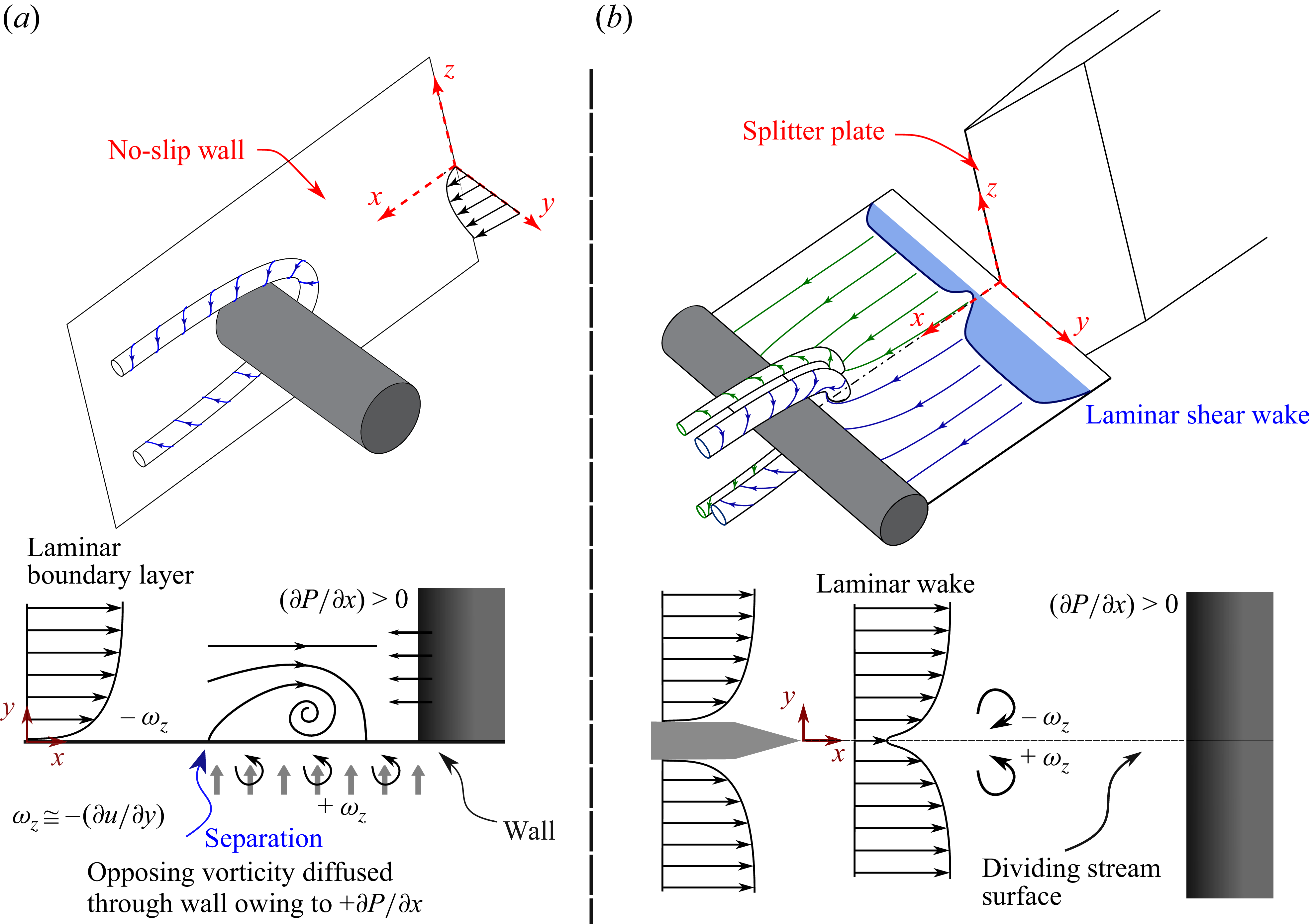
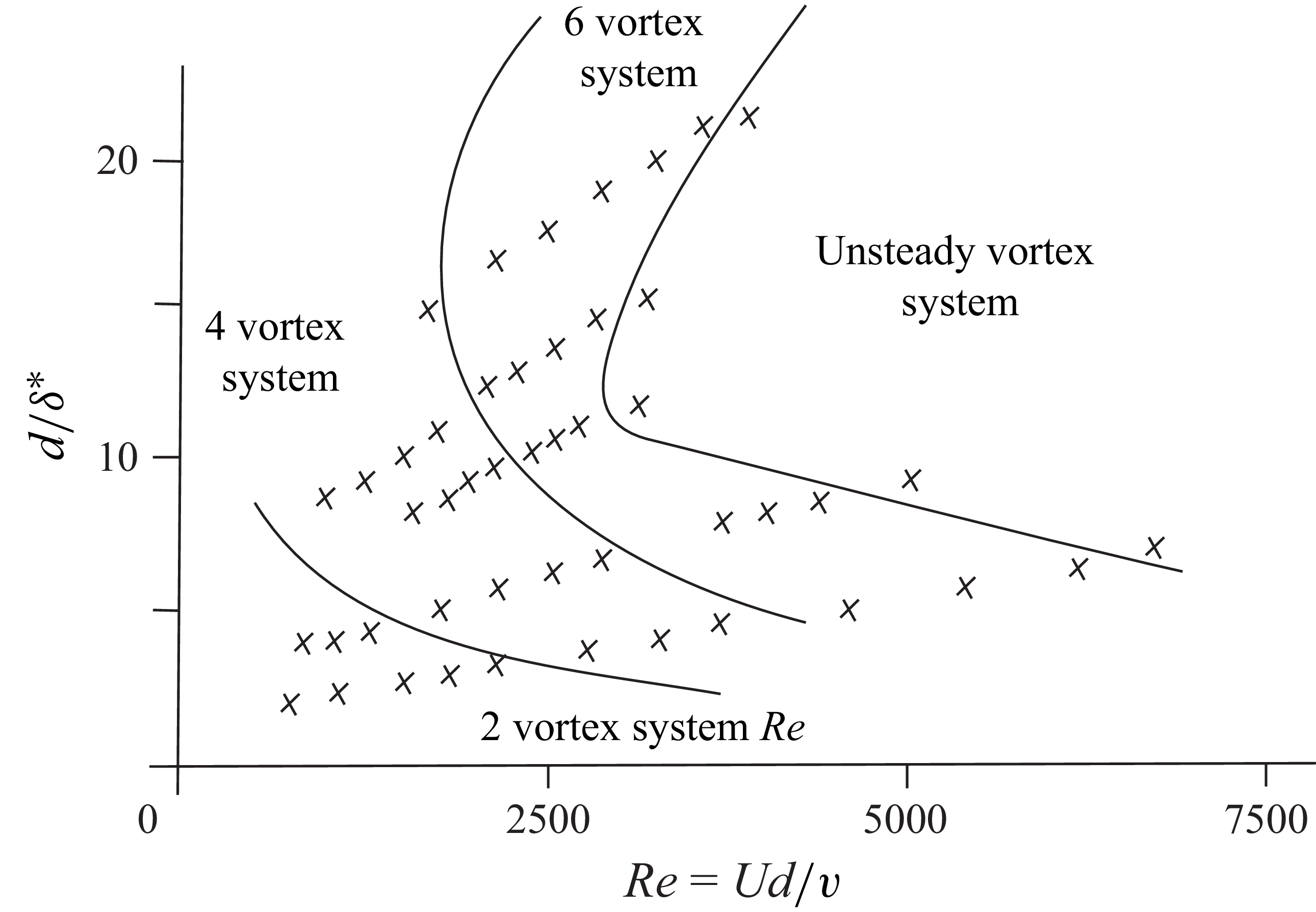


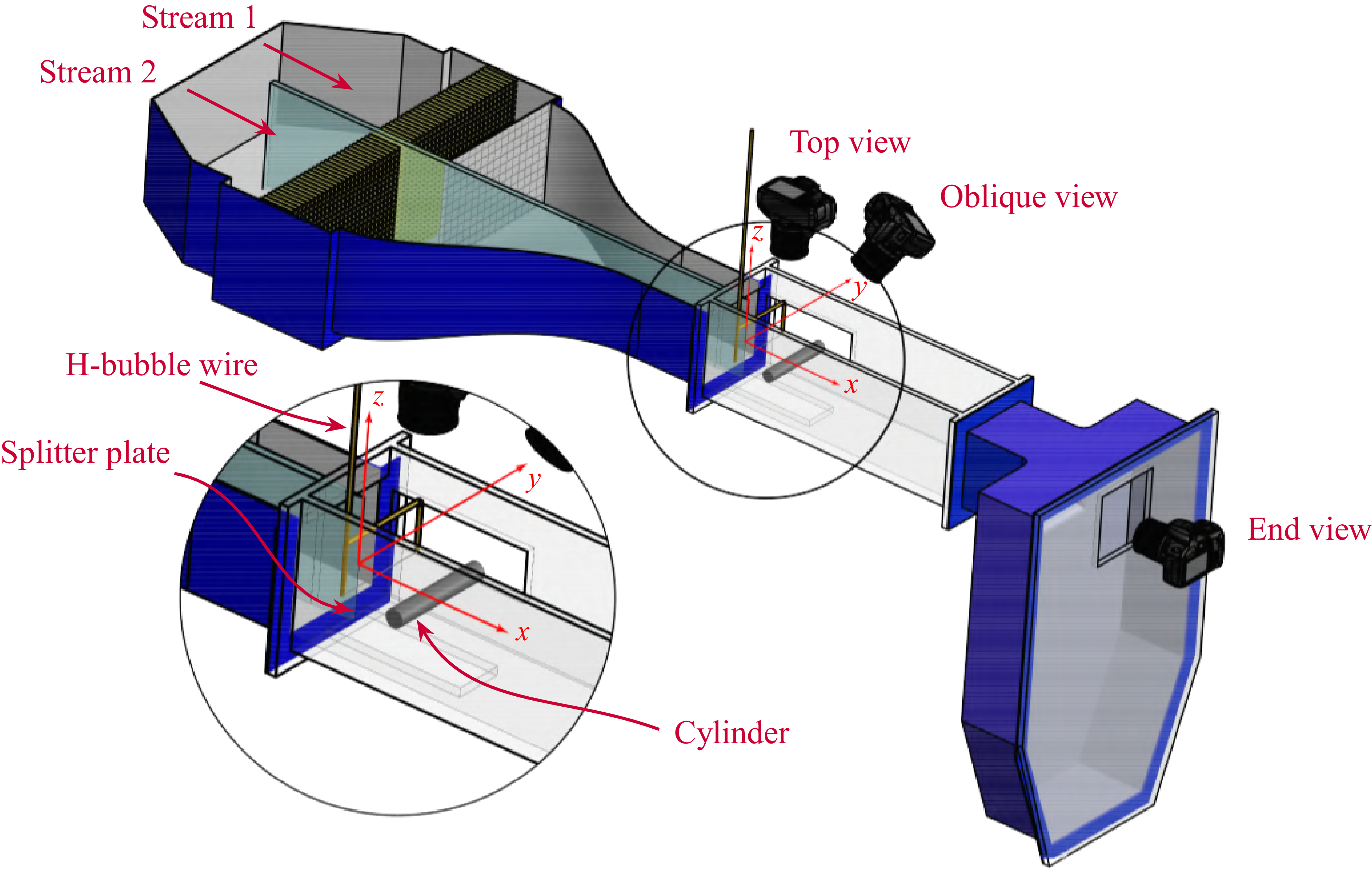

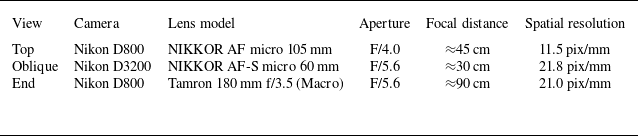
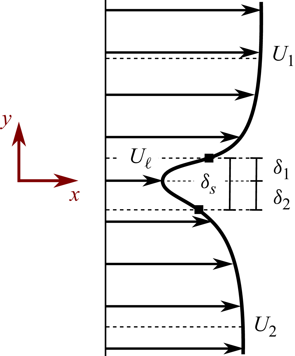


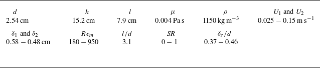
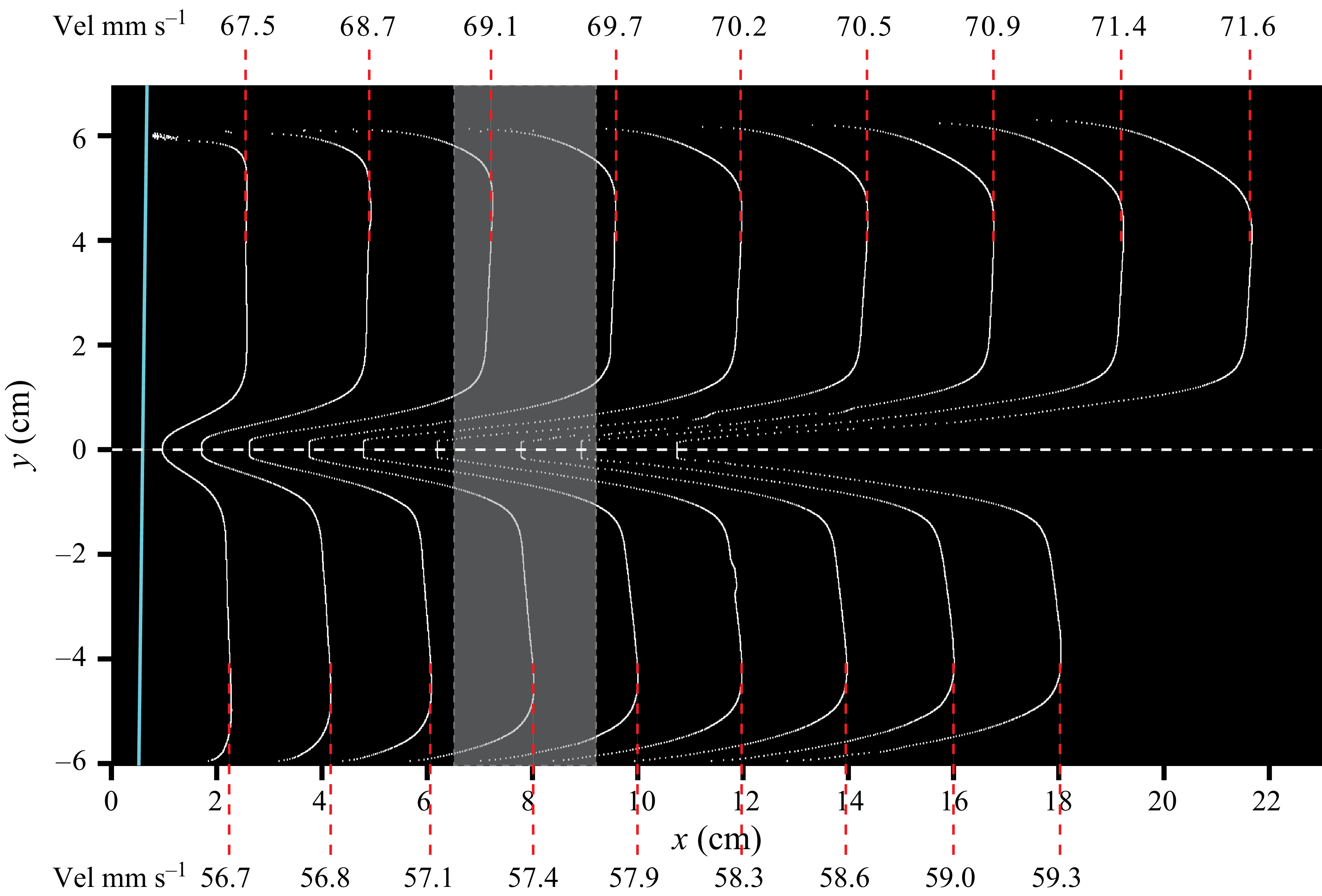


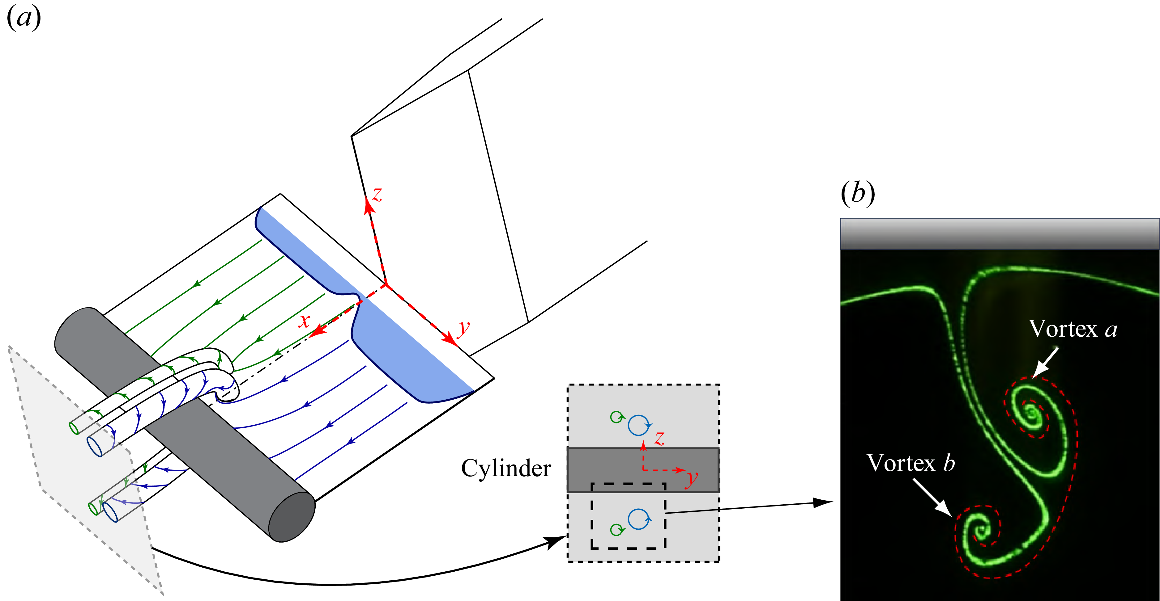


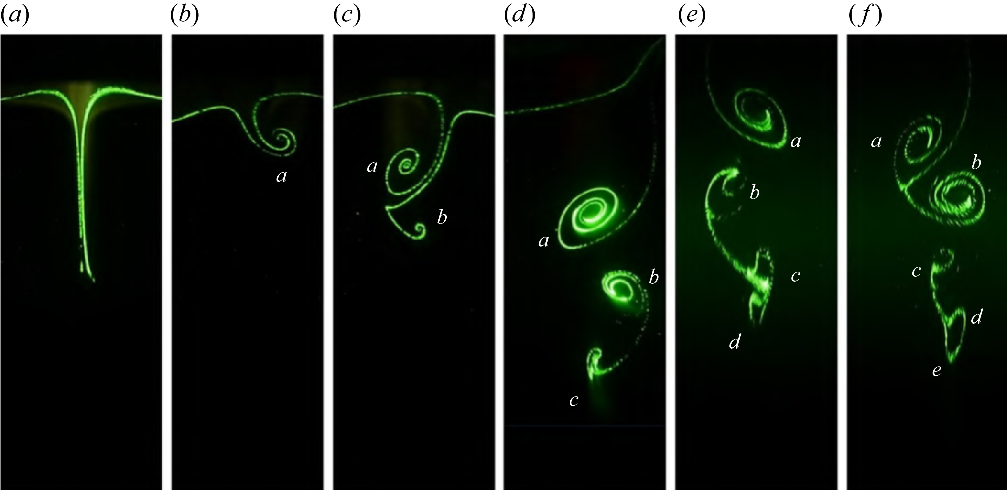


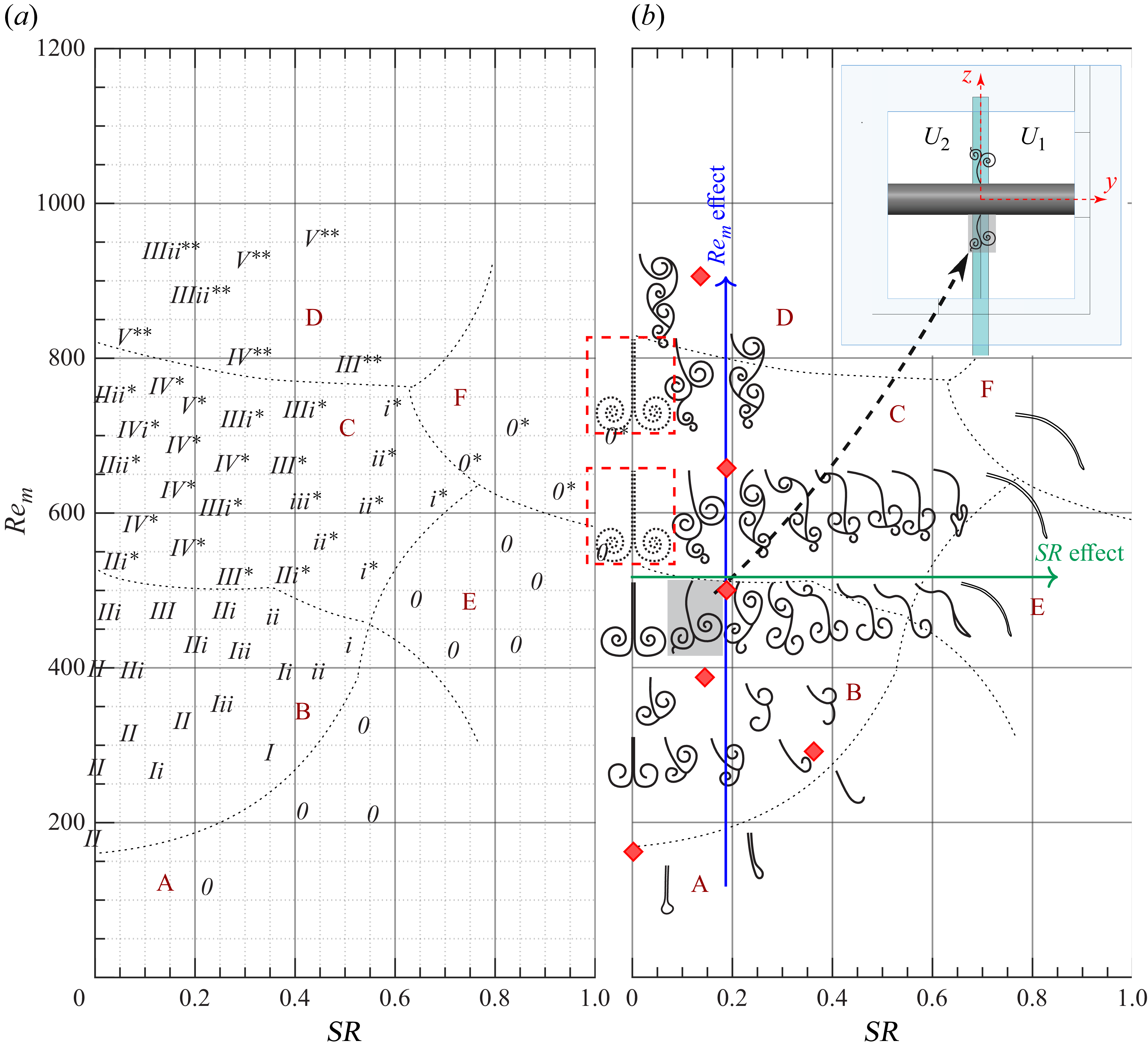


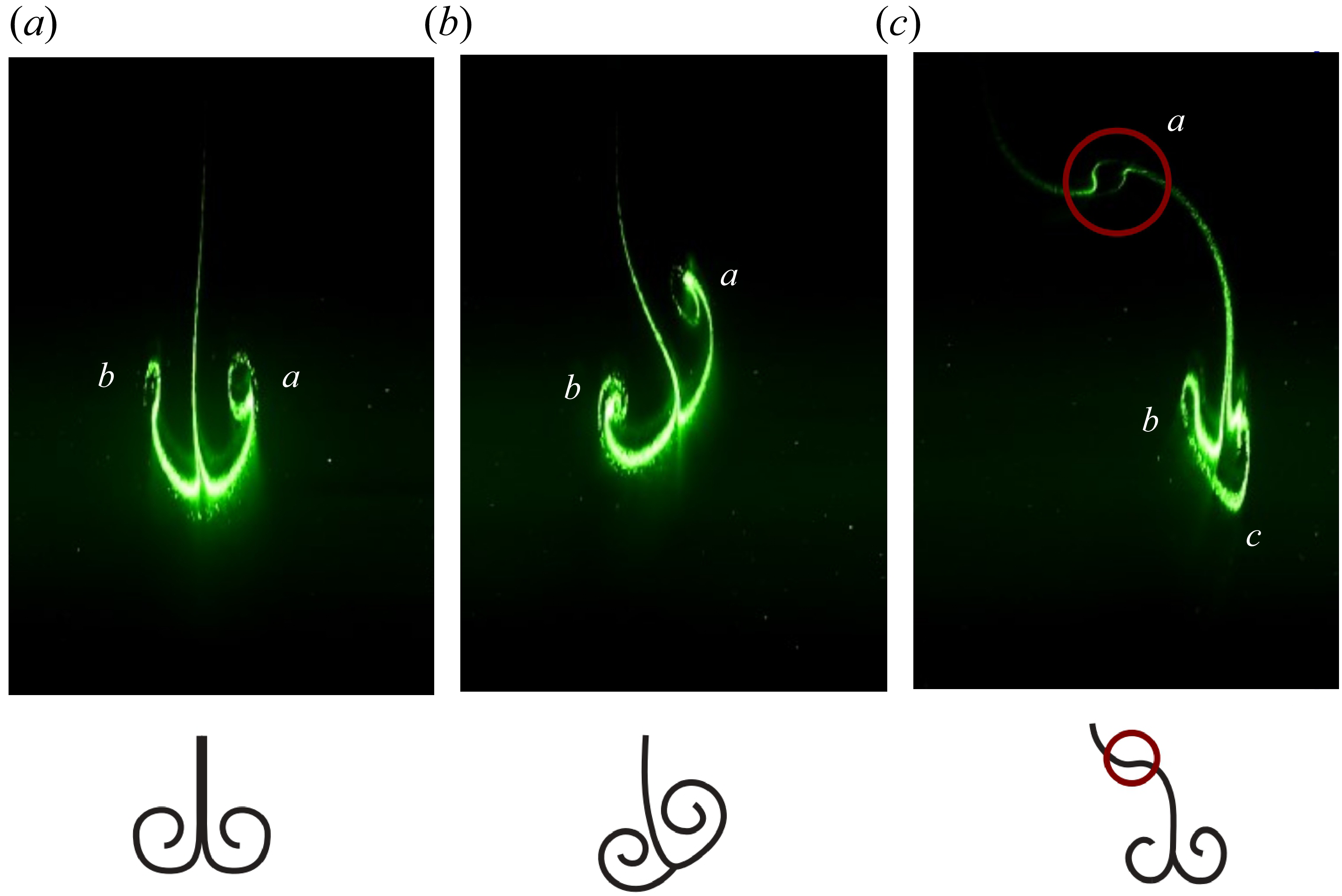


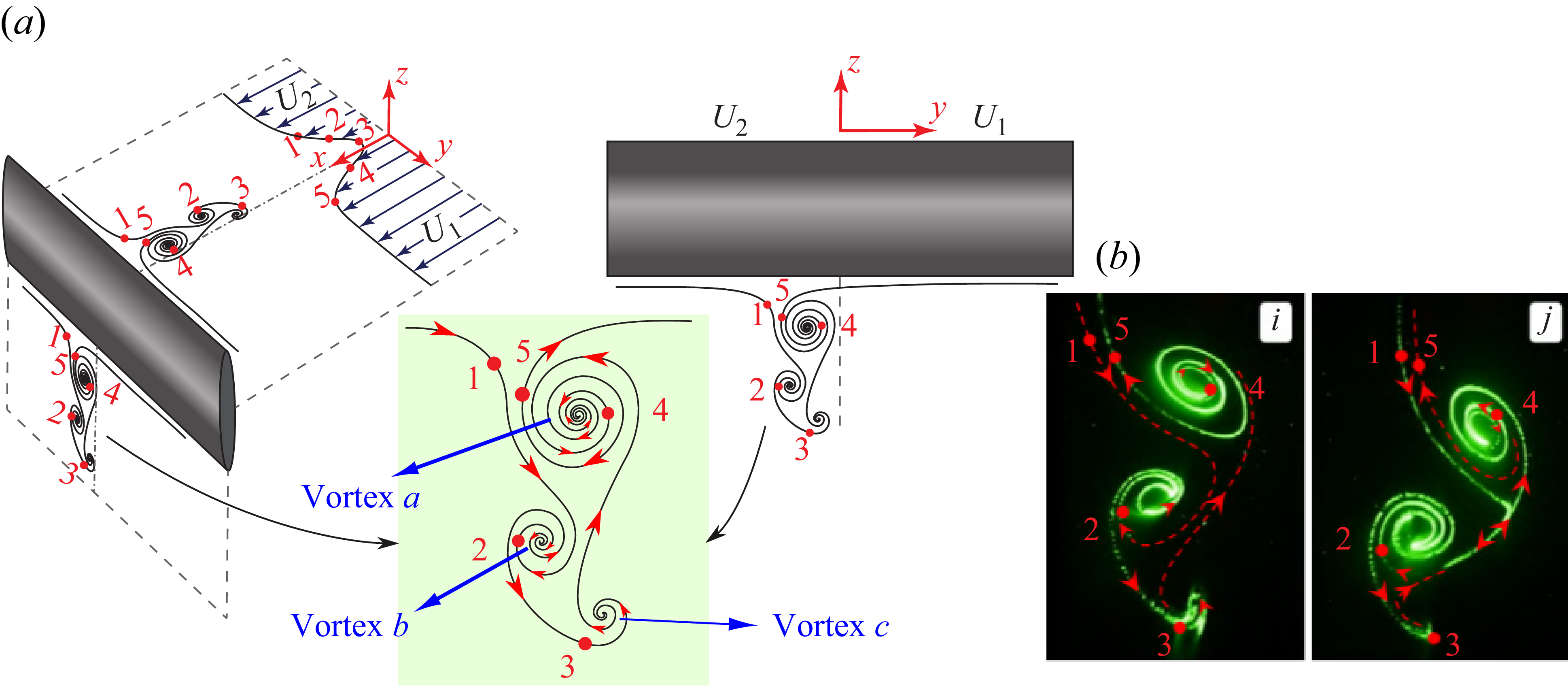


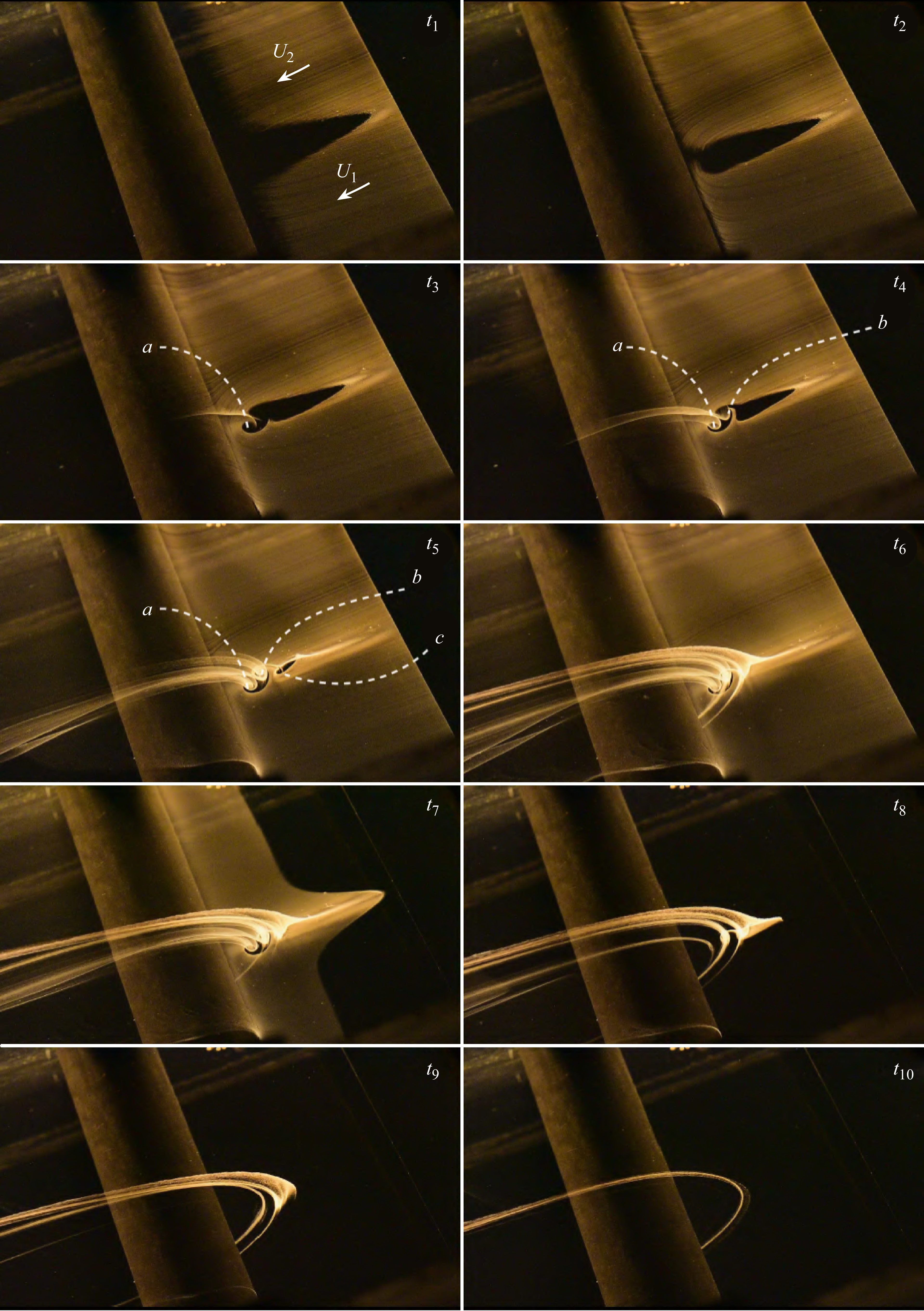


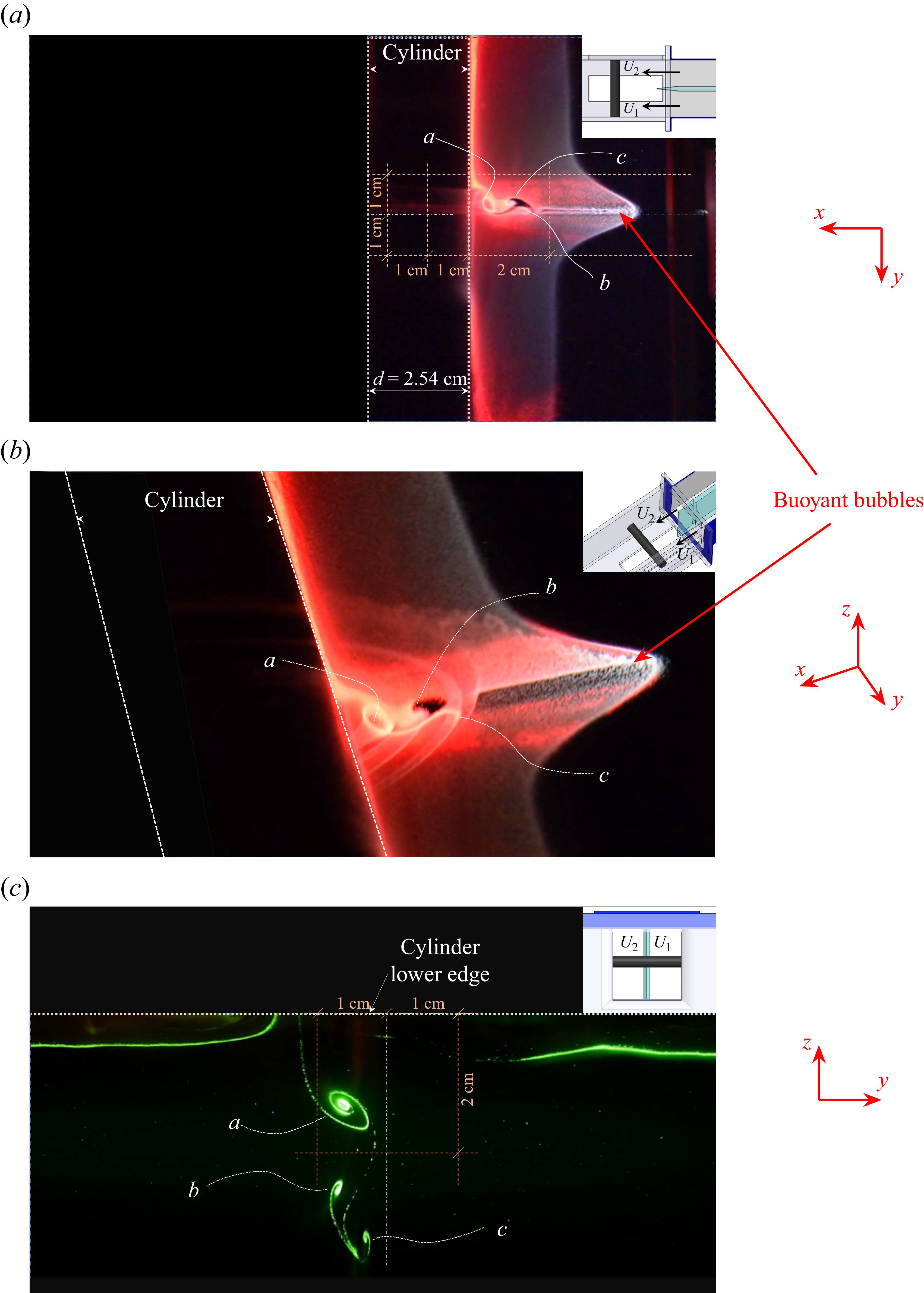


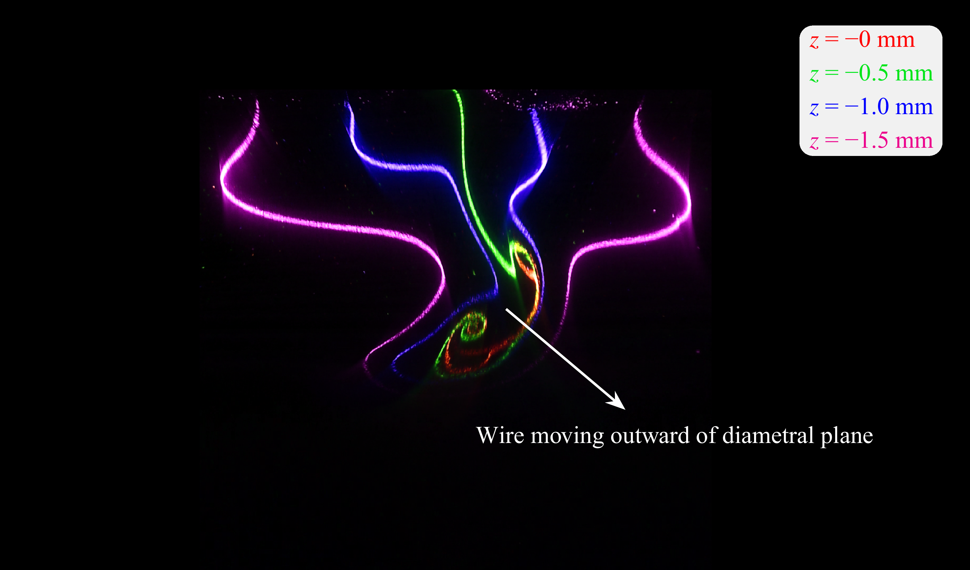


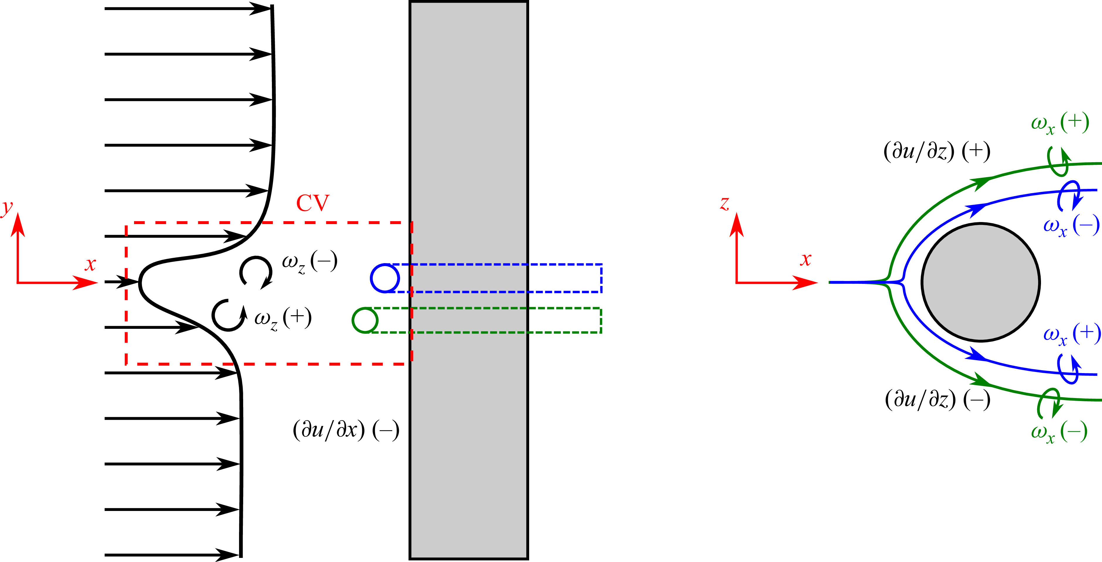
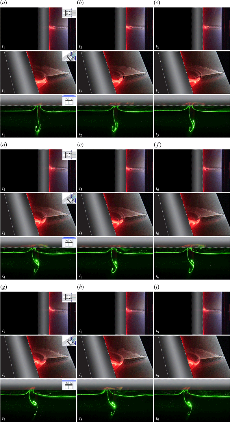


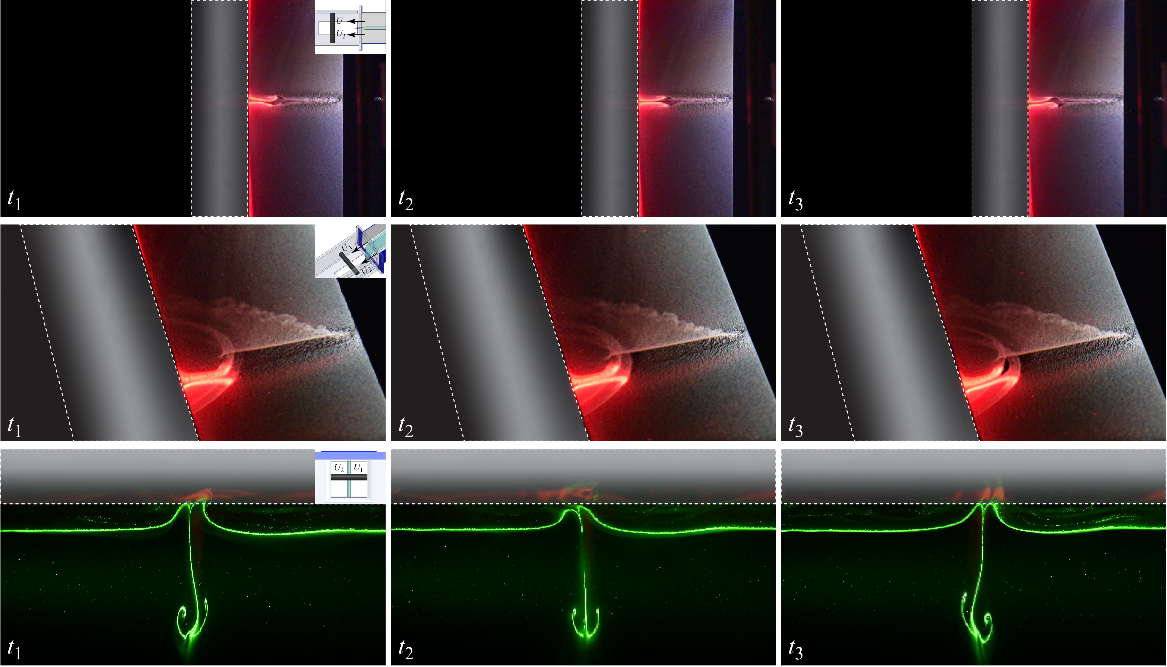


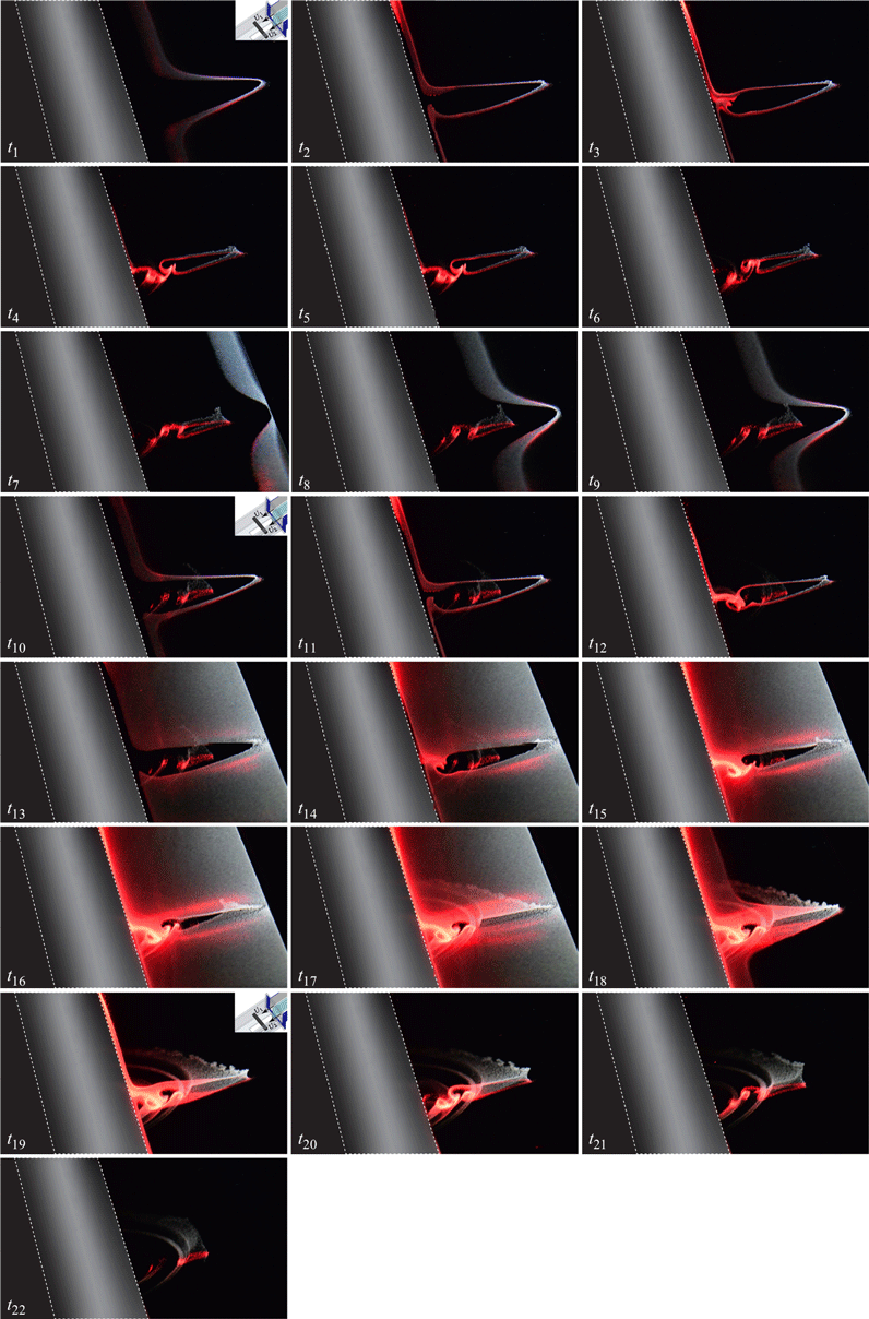


 Open access