


1. Introduction
A tsunami is an impulsive water wave, produced by a vertical displacement of ocean water surface as a result of earthquakes, underwater mass failures, subaerial landslides, volcanic activities or meteorite impacts. It is characterized as a shallow-water wave with a long wavelength but relatively small amplitude propagating in the ocean. Tsunami waves commonly carry enormous energy and have a potential to cause many deaths and significant property damage in coastal areas. Mega tsunamis have frequently struck the world's coastlines in recent years, for example, the Sumatra Tsunami (December 2004), the Chile Tsunami (February 2010), the Tohoku tsunami (March 2011) and, most recently, the Sulawesi tsunami (September 2018). Particularly, the 2004 Sumatra Tsunami killed nearly 230 000 people in 14 South Asian countries and has been known as one of the deadliest natural disasters in the recorded human history (Synolakis & Bernard Reference Synolakis and Bernard2006). Since then, the study of long-wave (e.g. tsunami) propagation in shallow water has attracted more attention.
Submarine bathymetry can have a significant impact on tsunami propagation, reflected by not only the shoaling effect due to the change in water depth but also ‘bending’ the wave's path due to refraction or diffraction. Oceanic ridges are a common type of topographic feature in the ocean basins. Previous studies on tsunami propagation have revealed that an oceanic ridge can guide and transmit tsunami waves from its source over tens of thousands of kilometres, causing disasters in faraway coastal areas. Woods & Okal (Reference Woods and Okal1987) applied a ray-tracing method to reconstruct the 1960 Chilean tsunami wave field, in which the most salient feature was the strongly focused energy field extending to northwest across the Pacific towards the Japanese and Kurile coasts due to the combined effect of the East Pacific Rise, Chile Rise and Tuamotu plateau. Through global tsunami propagation modelling, Titov et al. (Reference Titov, Rabinovich, Mofjeld, Thomson and González2005) demonstrated how the mid-ocean ridges guided the 2004 Sumatra tsunami and efficiently transmitted the enormous wave energy from its source to the far-field regions along the Pacific and Atlantic coasts of North America. Kowalik et al. (Reference Kowalik, Horrillo, Knight and Logan2008) showed that the energy field of the 2006 Kuril tsunami was redistributed by the trapping effect of the Koko Guyot and Hess Rise in the North Pacific Ocean, resulting in a second large wave packet arriving in the Crescent City 2–3 hours later. Song et al. (Reference Song, Fukumori, Shum and Yi2012) used satellite altimetry to examine the travelling patterns of the 2011 Tohoku tsunami and confirmed that the refraction effect of ocean ridges and seamount chains in the Pacific Ocean induced tsunami jets with larger amplitudes than elsewhere. Although both the observations and modelling results have started to shed light on such a wave-trapping phenomenon, the dynamic properties of the induced trapped waves are still poorly understood and relevant research is still in the early stage.
Recently, researchers have attempted to investigate the role of oceanic ridges in the propagation of long waves and use it to explain the delayed arrival of some devastating tsunami waves. According to Rabinovich, Woodworth & Titov (Reference Rabinovich, Woodworth and Titov2011) and Rabinovich, Candella & Thomson (Reference Rabinovich, Candella and Thomson2011), a tsunami guided by an ocean ridge usually contains two or more distinct trains with different spectral characteristics. The first train, travelling through the fastest route across the ocean, is usually small or even undetectable. On the other hand, the second train, typically having higher amplitude, can propagate as trapped waves along ocean ridges and follow a slower but more energy-conserving route to create catastrophic impacts. This phenomenon is sometimes referred to as ‘tsunami coda’ in the literature (Saito et al. Reference Saito, Inazu, Tanaka and Miyoshi2013). Although the phenomenon of tsunami coda has been widely recognized, it still lacks a rigorous theory to describe the detailed wave characteristics.
Preliminary study of trapped waves along ridge structures may be traced back to Ursell (Reference Ursell1951), who demonstrated that a trapped wave mode could exist over a submerged circular cylinder with a sufficiently small radius. But Jones (Reference Jones1953) later on argued that trapped wave modes might be created by a submerged cylinder of any symmetrical cross-sectional profile although no analytical solution was presented in his study. Longuet-Higgins (Reference Longuet-Higgins1968) derived analytical solutions for the trapped waves over a ridge with a step-like profile, based on which the changes of phase velocity and group velocity against the wavenumber were further analysed. It should be mentioned that the existence of trapped waves over a discontinuous topography is due to the multiple reflections created between the abrupt topographic boundaries. The dynamic mechanism is different from the refraction effect over a continuous bed that creates trapped rays turning back to the caustic lines parallel to the ridge. Buchwald (Reference Buchwald1968) analysed the trapped waves over a ridge of an arbitrary profile by numerically solving the long-wave equations with a variational approach. Shaw & Neu (Reference Shaw and Neu1981) presented analytical solutions based on two Kummer functions to describe trapped waves over a triangular ridge, but the solutions were implicit and must be further solved numerically. Most recently, Zheng et al. (Reference Zheng, Xiong and Wang2016) derived the analytical solutions for trapped waves over a submerged ridge with a symmetrical parabolic profile. However, the solutions are incomplete as they only consider symmetrical trapped waves but omit the anti-symmetrical components. Besides, although the variation of water depth is continuous over the adopted ridge profile, its derivative is discontinuous at the ridge top and so the resulting solutions are not suited to ridges with a slowly varying profile on the top.
Despite the noticeable attempts as mentioned above to analytically investigate the trapped wave dynamics induced by oceanic ridges, most of these existing studies are based on various simplified assumptions and have their limitations. First of all, various assumptions and approximations were introduced in the previous studies to necessarily simplify the theoretical analysis. Ursell (Reference Ursell1951) assumed the submerged cylinder is much smaller than the wavelength, which is not appropriate for analysing trapped waves excited by a tsunami for which the wavelength is commonly smaller than the scale of the ridge. Besides, the rigid-lid approximation is usually adopted in the investigation of trapped waves of periods of several days (Buchwald & Adams Reference Buchwald and Adams1968; Smith Reference Smith1970; Huthnance Reference Huthnance1975), which is also not suitable for tsunami waves that usually have periods less than a couple of hours. Secondly, some of previous studies only provided implicit formulations, which required numerical solutions to close up the theoretical frameworks and discuss the general nature of the problem (Jones Reference Jones1953; Buchwald Reference Buchwald1968; Huthnance Reference Huthnance1975). In some cases, even though explicit solutions described by transcendental functions were provided for trapped waves over special ridge profiles, the related dispersion equations were still implicit and again needed to be solved numerically (Shaw & Neu Reference Shaw and Neu1981; Zheng et al. Reference Zheng, Xiong and Wang2016). The reliance on numerical solutions may make the theoretical analysis framework less rigorous and limit its capability in providing a comprehensive and systemic analysis of the trapped wave dynamics. Finally, some existing analytical solutions are found to be incomplete as they only consider the symmetrical wave modes but omit the anti-symmetrical modes for trapped waves over a symmetrical ridge profile (Ursell Reference Ursell1951; Zheng et al. Reference Zheng, Xiong and Wang2016). Therefore, more research effort is still needed to develop more comprehensive analytical formulations to overcome the mentioned limitations and uncover the formation mechanisms and dynamic properties of tsunami-induced trapped waves over ocean ridges.
In this work, we will present new solutions to describe both symmetrical and anti-symmetrical trapped waves over a submerged ridge with a hyperbolic-cosine squared profile which may be used to better characterize the cross-sectional profiles of many real-world ocean ridges. For example, aseismic ridges, such as the Ninety East Ridge in the Indian Ocean and the Hawaii Ridge in the Central Pacific, are characterized by steep volcanic side slopes and flat tops, which may be idealized as a hyperbolic profile (Killworth Reference Killworth1989). The adopted hyperbolic-cosine squared profile also allows (i) derivation of analytical solutions with continuous water depth and derivatives over the whole profile (i.e. avoiding dividing solutions in different regions as reported in the previous studies, e.g. Zheng et al. (Reference Zheng, Xiong and Wang2016); (ii) the resulting trapped waves to be described by special functions with explicit analytical solutions (i.e. effectively avoiding numerical solutions as required in the previous studies, e.g. Buchwald (Reference Buchwald1968), Shaw & Neu (Reference Shaw and Neu1981); and (iii) the related dispersion relationships to be expressed as algebraic equations, enabling explicit quantification of their sensitivity to the topographic profile. A ray-tracing method is also applied to provide further physical insights into the wave-trapping processes. Finally, a validated Boussinesq wave model is used to conduct numerical experiments to demonstrate the wave-trapping process induced by tsunamis on the adopted submerged ridge and confirm the validity of the new analytical solutions.
2. New analytical solutions
Figure 1 illustrates the problem under consideration in a three-dimensional Cartesian coordinate system, in which a section of a straight ridge of infinite length is assumed to have a hyperbolic-cosine squared cross-sectional profile. With the y-axis coinciding with the central line of the ridge and x-axis crossing the profile, the resulting bathymetry is given by
 \begin{equation}h(x) = {h_0}\ {\cosh ^2}(\lambda x),\end{equation}
where λ (m−1) is a parameter determining the shape of the ridge profile (i.e. profile parameter) and h 0 is the still water depth above the ridge top.
Hyperbolic-cosine squared spine profile.

2.1. Derivation
A tsunami is typically a long wave with water depth much smaller than wavelength and can be mathematically described by the linear shallow-water equations (SWE), which include the linearized momentum equations for free long waves
 \begin{equation}\frac{{\partial u}}{{\partial t}} + g\frac{{\partial \eta }}{{\partial x}} = 0,\end{equation}
and
 \begin{equation}\frac{{\partial v}}{{\partial t}} + g\frac{{\partial \eta }}{{\partial y}} = 0,\end{equation}
and the continuity equation
 \begin{equation}\frac{{\partial \eta }}{{\partial t}} + \frac{{\partial (hu)}}{{\partial x}} + \frac{{\partial (hv)}}{{\partial y}} = 0,\end{equation}
where η is the free surface elevation, u and v are the velocity components in the x and y-directions, g is the acceleration due to gravity and t is the time. For shelf waves associated with barometric pressure changes and having periods of greater than or equal to 1 day, the Coriolis effect should be considered in (2.2) and (2.3), but the time derivative of the free surface elevation in (2.4) may be neglected following the rigid-lid approximation (Buchwald & Adams Reference Buchwald and Adams1968; Smith Reference Smith1970). However, for the tsunami waves as considered in this study, their periods are usually less than a couple of hours and hence the Coriolis effect is negligible and the time derivative term in (2.4) should be retained.
Combining (2.2)–(2.4), the governing equation for η can be obtained as follows
 \begin{equation}\frac{{{\partial ^2}\eta }}{{\partial {t^2}}} - g\left[ {\frac{\partial }{{\partial x}}\left( {h\frac{{\partial \eta }}{{\partial x}}} \right) + \frac{\partial }{{\partial y}}\left( {h\frac{{\partial \eta }}{{\partial y}}} \right)} \right] = 0.\end{equation}
For periodic trapped waves, the solution for η may be formulated as
 \begin{equation}\eta (x,y,t) = \zeta (x)\exp [\textrm{i}({k_y}y - \omega t)],\end{equation}
in which ω is the angular frequency of the incident wave, ky is the wave vector component in the y-direction and i = (−1)1/2. Substituting (2.6) into (2.5) and considering the depth profile as defined in (2.1), we have
 \begin{equation}\frac{{{\textrm{d}^2}\zeta }}{{\textrm{d}{x^2}}} + 2\lambda \tanh (\lambda x)\frac{{\textrm{d}\zeta }}{{\textrm{d}\kern0.06em x}} + \frac{{{\omega ^2}}}{{g{h_0}}}{\,{\rm sech}\, ^2}(\lambda x)\zeta - k_y^2\zeta = 0.\end{equation}
The above equation is specifically obtained for a ridge with a hyperbolic-cosine squared profile since the depth profile in (2.1) has been taken into account. The generalized equation for trapped waves over a ridge of an arbitrary profile can be found in Buchwald (Reference Buchwald1968). However, rather than transforming the equation into an integral form for numerical solution as proposed by Buchwald (Reference Buchwald1968), (2.7) is transformed into a transcendental equation to directly find the analytical solution.
To simplify the expression, we introduce a new independent variable
 \begin{equation}\chi = \tanh (\lambda x),\end{equation}
and a new dependent variable
 \begin{equation}f(\chi ) = \frac{\zeta }{{\sqrt {1 - {\chi ^2}} }}.\end{equation}
Using these new variables, (2.7) reduces to
 \begin{equation}(1 - {\chi ^2})\frac{{{\textrm{d}^2}f}}{{\textrm{d}{\chi ^2}}} - 2\chi \frac{{\textrm{d}f}}{{\textrm{d}\chi }} + \left[ {\nu (\nu + 1) - \frac{{{\mu^2}}}{{1 - {\chi^2}}}} \right]f = 0.\end{equation}
This is essentially the associated Legendre differential equation of degree ν and order μ, with
 \begin{equation}v = - \frac{1}{2} \pm \sqrt {\frac{1}{4} + \frac{{{\omega ^2}}}{{g{h_0}{\lambda ^2}}}} ,\end{equation}
and
 \begin{equation}\mu = \sqrt {1 + {{\left( {\frac{{{k_y}}}{\lambda }} \right)}^2}} .\end{equation}
The general solution to (2.10) may be expressed as
 \begin{equation}f = A \cdot P(v,\mu ,\chi ) + B \cdot Q(v,\mu ,\chi ),\end{equation}
where A and B are constants, and P and Q are the two linearly independent associated Legendre functions given by Olver et al. (Reference Olver, Lozier, Boisvert and Clark2010)
 \begin{equation}P(v,\mu ,\chi ) = \frac{1}{{\varGamma (1 - \mu )}}{\left( {\frac{{1 + \chi }}{{1 - \chi }}} \right)^{\mu /2}}F\left( { - v,v + 1,1 - \mu ,\frac{{1 - \chi }}{2}} \right),\end{equation}
and
 \begin{equation}Q(v,\mu ,\chi ) = \frac{{{\rm \pi} }}{{2\sin \mu {{\rm \pi} }}}\left\{ {\cos (\mu {{\rm \pi} })P(v,\mu ,\chi ) - \frac{{\varGamma (v + \mu + 1)}}{{\varGamma (v - \mu + 1)}}P(v, - \mu ,\chi )} \right\},\end{equation}
in which F is a hypergeometric function defined as
 \begin{equation}F(a,b,c,\tau ) = \sum\limits_{s = 0}^\infty {\frac{{{{(a)}_s}{{(b)}_s}}}{{{{(c)}_s}s!}}} {\tau ^s},\end{equation}
where a, b and c are real parameters, and τ is a real variable, with
 \begin{equation}{(a)_s} = a(a + 1)(a + 2) \cdots (a + s - 1).\end{equation}
Here,  $\varGamma$ is a gamma function expressed as follows
 \begin{equation}\varGamma (\tau ) = \int_0^\infty {\exp ( - t){t ^{\tau - 1}}\,\textrm{d}t} .\end{equation}
For the above associated Legendre functions, we have
 \begin{equation}P( - \nu - 1,\mu ,\chi ) = P(\nu ,\mu ,\chi ),\end{equation}
and
 \begin{equation}Q( - \nu - 1,\mu ,\chi ) = \frac{{\sin [(\nu + \mu ){{\rm \pi} }]Q(\nu ,\mu ,\chi ) - {{\rm \pi} }\cos (\nu {{\rm \pi} })\cos (\mu {{\rm \pi} })P(\nu ,\mu ,\chi )}}{{\sin [(\nu - \mu ){{\rm \pi} }]}},\end{equation}
which implies that  $A \cdot P( - \nu - 1,\mu ,\chi ) + B \cdot Q( - \nu - 1,\mu ,\chi )$ and $A \cdot P(\nu ,\mu ,\chi ) + B \cdot Q(\nu ,\mu ,\chi )$ are linearly dependent; hence the degree ν can be defined as follows
 \begin{equation}\nu = - \frac{1}{2} + \sqrt {\frac{1}{4} + \frac{{{\omega ^2}}}{{g{h_0}{\lambda ^2}}}} .\end{equation}
Finally, for the trapped waves over the hyperbolic-cosine squared oceanic ridge, we have
 \begin{equation}\zeta = sech (\lambda x)[A \cdot P(v,\mu ,\chi ) + B \cdot Q(v,\mu ,\chi )].\end{equation}
Due to the fact that the associated Legendre functions are a set of orthogonal functions (Olver et al. Reference Olver, Lozier, Boisvert and Clark2010), (2.22) gives a complete and orthogonal solution for the trapped waves over the specific type of symmetrical ridge as considered.
Due to the infinite width of the ridge, the trapped waves are assumed to focus on the topography and so the wave amplitude should approach to zero at infinity, i.e.
 \begin{equation}\zeta {|_{|x|= \infty }} \to 0.\end{equation}
The associated Legendre functions have an asymptotic singularity as x → ∞, where χ = tanh(λx) → 1−, leading to
 \begin{equation}P(v,\mu ,\chi )\sim \frac{1}{{\varGamma (1 - \mu )}}{\left( {\frac{2}{{1 - \chi }}} \right)^{\mu /2}},\end{equation}
and
 \begin{equation}Q(v,\mu ,\chi )\sim \frac{1}{2}\cos (\mu {{\rm \pi} }) \cdot \varGamma (\mu ){\left( {\frac{2}{{1 - \chi }}} \right)^{\mu /2}}.\end{equation}
Thus, the free surface over the ridge becomes
 \begin{equation}\zeta (\chi \to {1^ - }) = {2^{\mu /2}}{(1 + \chi )^{1/2}}{(1 - \chi )^{(1 - \mu )/2}}\left[ {A\frac{{\sin (\mu {{\rm \pi} })}}{{{\rm \pi} }} + \frac{B}{2}\cos (\mu {{\rm \pi} })} \right]\varGamma (\mu ).\end{equation}
As μ > 1, the term  ${(1 - \chi )^{(1 - \mu )/2}}$ on the right-hand side tends to infinity unless
 \begin{equation}A\frac{{\sin (\mu {{\rm \pi} })}}{{{\rm \pi} }} + \frac{B}{2}\cos (\mu {{\rm \pi} }) = 0,\end{equation}
i.e.
 \begin{equation}B = - \frac{2}{{{\rm \pi} }}\tan (\mu {{\rm \pi} })A.\end{equation}
So the trapped waves over a hyperbolic-cosine squared ridge can be described as
 \begin{equation}\zeta = A \cdot \,{\rm sech}\, (\lambda x)\left\{ {P[\nu ,\mu ,\tanh (\lambda x)] - \frac{2}{{{\rm \pi} }} \cdot \tan (\mu {{\rm \pi} }) \cdot Q[\nu ,\mu ,\tanh (\lambda x)]} \right\},\end{equation}
in which A is the wave amplitude at the top of the ridge.
The relationship between μ and ν is determined by the boundary conditions at the ridge top (x = 0). Continuity of water surface and velocity requires
 \begin{equation}\zeta {|_{x = {0^ - }}} = \zeta {|_{x = {0^ + }}},\end{equation}
and
 \begin{equation}u{|_{x = {0^ - }}} = u{|_{x = {0^ + }}}.\end{equation}
Equation (2.31) may also be viewed as the continuity of mass as the water depth is continuous.
As revealed by Buchwald (Reference Buchwald1968) and Shaw & Neu (Reference Shaw and Neu1981), the motion of the free surface over a ridge of symmetrical topographic profile, regardless whether it is continuous or not, can be separated into symmetrical and anti-symmetrical patterns. The corresponding solutions for these two classes of wave motions will be discussed in detail as follows.
(a) Class I: symmetrical wave pattern
Symmetrical motion of free surface requires ζ to be an even function of x, i.e.
 \begin{equation}{\left. {\frac{{\textrm{d}\zeta }}{{\textrm{d}\kern0.06em x}}} \right|_{x = 0}} = 0,\end{equation}
which gives
 \begin{equation}P(v + 1,\mu ,0) - \frac{2}{{{\rm \pi} }}\tan (\mu {{\rm \pi} })Q(v + 1,\mu ,0) = 0.\end{equation}
The corresponding associated Legendre functions at x = 0 are
 \begin{equation}P(v,\mu ,0) = \frac{{{2^\mu }{{{\rm \pi} }^{1/2}}}}{{\varGamma ({\textstyle{1 \over 2}}v - {\textstyle{1 \over 2}}\mu + 1)\varGamma ({\textstyle{1 \over 2}} - {\textstyle{1 \over 2}}v - {\textstyle{1 \over 2}}\mu )}},\end{equation}
and
 \begin{equation}Q(v,\mu ,0) = - \frac{{{2^{\mu - 1}}{{{\rm \pi} }^{1/2}}\sin [{\textstyle{1 \over 2}}(\mu + v){{\rm \pi} }]\varGamma ({\textstyle{1 \over 2}}v + {\textstyle{1 \over 2}}\mu + {\textstyle{1 \over 2}})}}{{\varGamma ({\textstyle{1 \over 2}}v - {\textstyle{1 \over 2}}\mu + 1)}}.\end{equation}
Equation (2.33) can be rewritten as
 \begin{equation}\tan [{\textstyle{1 \over 2}}(v + \mu ){{\rm \pi} }] = \tan (\mu {{\rm \pi} }),\end{equation}
which is equivalent to
 \begin{equation}v = \mu + 2m\quad m = 0,1,2 \ldots .\end{equation}
Substituting (2.12) and (2.21) into (2.37) leads to
 \begin{equation}{\omega ^2} = g{h_0}(\sqrt {{\lambda ^2} + k_y^2} + 2m\lambda )[\sqrt {{\lambda ^2} + k_y^2} + (2m + 1)\lambda ],\end{equation}
where m is a non-negative integer representing the cross-sectional mode number. The above equation determines the relationship between the wave frequency and the wavenumber, which may be referred to as the dispersion equation. The dispersion relationship describes how the propagating trapped waves of different frequencies or modes separate or ‘disperse’ according to their wave speeds. The corresponding phase velocity and group velocity c and cg are given by
 \begin{gather}c = \frac{\omega }{{{k_y}}} = \frac{{\dfrac{\omega }{\lambda }}}{{\sqrt {{{\left[ {\sqrt {\dfrac{{{\omega^2}}}{{g{h_0}{\lambda^2}}} + \dfrac{1}{4}} - 2m - \dfrac{1}{2}} \right]}^2} - 1} }},\end{gather}
 \begin{gather}{c_g} = \frac{{\textrm{d}\omega }}{{\textrm{d}{k_y}}} = c \cdot \frac{{\sqrt {\dfrac{{{\omega ^2}}}{{g{h_0}{\lambda ^2}}} + \dfrac{1}{4}} \cdot \left\{ {{{\left[ {\sqrt {\dfrac{{{\omega^2}}}{{g{h_0}{\lambda^2}}} + \dfrac{1}{4}} - 2m - \dfrac{1}{2}} \right]}^2} - 1} \right\}}}{{\dfrac{{{\omega ^2}}}{{g{h_0}{\lambda ^2}}} \cdot \left[ {\sqrt {\dfrac{{{\omega^2}}}{{g{h_0}{\lambda^2}}} + \dfrac{1}{4}} - \left( {2m + \dfrac{1}{2}} \right)} \right]}} = c \cdot n,\end{gather}
where n may be referred to as the group velocity factor.
As the phase velocity of a propagating wave must be real, it requires the expression inside the square root of (2.39) to be greater than zero, which yields
 \begin{equation}m \lt \frac{1}{2}\sqrt {\frac{{{\omega ^2}}}{{g{h_0}{\lambda ^2}}} + \frac{1}{4}} - \frac{3}{4}.\end{equation}
This renders the finite number of possible trapped wave modes for Class I. The number of possible modes increases with increasing angular frequency ω but decreasing h 0 (water depth at the ridge top) and λ (profile parameter). Expression (2.41) can be also transformed to identify the cutoff values of ω, h 0 and λ for prescribed conditions. Furthermore, the dispersion relationship (2.38) indicates that ω increases with the mode number for a fixed wavenumber ky, h 0 and λ, and has its maximal values for mode 0, giving
 \begin{equation}{\omega ^2} = g{h_0}{\lambda ^2}\sqrt {1 + k_y^2/{\lambda ^2}} (\sqrt {1 + k_y^2/{\lambda ^2}} + 1) \gt 2g{h_0}{\lambda ^2},\end{equation}
i.e.
 \begin{equation}\omega \gt \sqrt {2g{h_0}} \lambda .\end{equation}
This defines the lower limit of the angular frequency ω for the Class I modes of trapped waves.
Obviously, (2.28) is undefined when μ = 1/2 + m as B approaches infinity. The corresponding wavenumber can be obtained from (2.12), i.e.
 \begin{equation}{k_y} = \lambda \sqrt {{{({\textstyle{1 \over 2}} + m)}^2} - 1} .\end{equation}
As the wavenumber for propagating waves must be real, it requires the term in the square root of (2.44) greater than 0, which in turn requires m to be an integral number, i.e. m = 1, 2, …. In this case, the free surface solution of the trapped waves can be expressed as
 \begin{equation}\zeta = B\sqrt {1 - {\chi ^2}} \cdot Q(v,m + {\textstyle{1 \over 2}},\chi ) = B\,{\rm sech}\, (\lambda x) \cdot Q[v,m + {\textstyle{1 \over 2}},\tanh (\lambda x)].\end{equation}
According to the symmetrical condition at the ridge top (2.32), we can then have
 \begin{equation}v = m - {\textstyle{1 \over 2}},\end{equation}
and from (2.21),
 \begin{equation}{\omega ^2} = ({m^2} - {\textstyle{1 \over 4}})g{h_0}{\lambda ^2}\quad m = 1,2, \ldots .\end{equation}
(b) Class II: anti-symmetrical wave pattern
Anti-symmetrical motion of the free surface implies that ζ is an odd function of x and must be equal to zero at x = 0, i.e.
 \begin{equation}\zeta {|_{x = 0}} = 0,\end{equation}
which gives
 \begin{equation}P[\nu ,\mu ,0] - \frac{2}{{{\rm \pi} }} \cdot \tan (\mu {{\rm \pi} }) \cdot Q[\nu ,\mu ,0] = 0.\end{equation}
Substituting (2.34) and (2.35) into (2.49) and using the following mathematical formula
 \begin{equation}\varGamma (z)\varGamma (1 - z) = {{\rm \pi} }/\sin ({{\rm \pi} }z),\end{equation}
the following equation is derived
 \begin{equation}\cos \frac{{(\mu - v){{\rm \pi} }}}{2} = 0.\end{equation}
This is equivalent to
 \begin{equation}v = \mu + 2m - 1\quad m = 1,2 \ldots .\end{equation}
Substituting (2.12) and (2.21) into (2.52), we have
 \begin{equation}{\omega ^2} = g{h_0}{\lambda ^2}(\sqrt {1 + k_y^2/{\lambda ^2}} + 2m)(\sqrt {1 + k_y^2/{\lambda ^2}} + 2m - 1).\end{equation}
This defines the dispersion relationship for the anti-symmetrical modes of the trapped waves. The corresponding phase velocity and group velocity can be subsequently derived and given as
 \begin{gather}c = \frac{\omega }{{{k_y}}} = \frac{{\omega /\lambda }}{{\sqrt {{{\left( {\sqrt {\dfrac{{{\omega^2}}}{{g{h_0}{\lambda^2}}} + \dfrac{1}{4}} - 2m + \dfrac{1}{2}} \right)}^2} - 1} }},\end{gather}
 \begin{gather}{c_g} = \frac{{\textrm{d}\omega }}{{\textrm{d}{k_y}}} = c \cdot \frac{{\sqrt {\dfrac{{{\omega ^2}}}{{g{h_0}{\lambda ^2}}} + \dfrac{1}{4}} \left( {\sqrt {\dfrac{{{\omega^2}}}{{g{h_0}{\lambda^2}}} + \dfrac{1}{4}} - 2m + \dfrac{3}{2}} \right)\left( {\sqrt {\dfrac{{{\omega^2}}}{{g{h_0}{\lambda^2}}} + \dfrac{1}{4}} - 2m - \dfrac{1}{2}} \right)}}{{\dfrac{{{\omega ^2}}}{{g{h_0}{\lambda ^2}}}\left( {\sqrt {\dfrac{{{\omega^2}}}{{g{h_0}{\lambda^2}}} + \dfrac{1}{4}} - 2m + \dfrac{1}{2}} \right)}}.\end{gather}
As the phase velocity for a propagating wave must be real, it requires the expression inside the square root of (2.54) to be greater than zero, which leads to
 \begin{equation}m \lt \frac{1}{2}\sqrt {\frac{{{\omega ^2}}}{{g{h_0}{\lambda ^2}}} + \frac{1}{4}} - \frac{1}{4}.\end{equation}
The above expression renders the finite number of possible trapped wave modes for Class II. The number of possible modes increases with increasing ω but decreasing h 0 and λ. Expression (2.56) can also be used to identify the cutoff values of ω, h 0 and λ for any prescribed conditions.
According to the dispersion relationship defined in (2.53), the frequency ω increases with the mode number for a fixed wavenumber ky, h 0 and λ, and has its maximum value for mode 1, leading to
 \begin{equation}{\omega ^2} = g{h_0}{\lambda ^2}(\sqrt {1 + k_y^2/{\lambda ^2}} + 2)(\sqrt {1 + k_y^2/{\lambda ^2}} + 1) \gt 6g{h_0}{\lambda ^2},\end{equation}
i.e.
 \begin{equation}\omega \gt \sqrt {6g{h_0}} \lambda ,\end{equation}
which defines the lower limit of ω for the Class II modes of trapped waves.
2.2. Dispersion relationship
Both (2.38) and (2.53) degenerate into the dispersion relationship of the linearized SWE on an even bed, i.e. ω = ky(gh)1/2 when λ = 0. In this case, there is no frequency dispersion, i.e. all waves will travel at the same speed. This essentially indicates that the dispersion of trapped waves of different frequencies/modes propagating at different speeds is a direct result of uneven bed profile. Therefore, (2.38) and (2.53) may be more appropriately referred to as the topography-dispersion relationships.
According to the dispersion relationships as defined in (2.38) and (2.53), the wavenumber ky is related to not only the frequency ω and water depth h 0, but also the cross-section profile parameter λ and the mode number m. It is therefore necessary to further investigate the sensitivity of the dispersion relationships to these parameters. For a fixed ky and m, the unique angular frequency ω may be determined by solving (2.38) or (2.53). Obviously, there are m different values of wavenumber ky for a fixed frequency ω. Accordingly, the corresponding solution may be referred to as mode m. The dispersion relationships imply that ω 2 increases linearly with h 0 when ky, λ and m are fixed. For given h 0 and λ, the frequency ω increases with the wavenumber ky and also with m for a specific wavenumber, as illustrated in figure 2. Furthermore, the frequency of the anti-symmetric waves is lower than the associated symmetric waves for given h 0, ky, λ and m. Possible explanation is that the anti-symmetric waves may be considered as a lower mode than the symmetric waves for the same mode number m because there are 2m − 1 node lines for the anti-symmetric wave pattern but 2m node lines for the symmetric wave pattern (the spatial distribution patterns of the trapped waves will be presented and discussed in § 2.3).
Non-dimensional dispersion relationships for trapped waves over a hyperbolic-cosine squared ridge.

Figures 3 and 4 respectively illustrate the behaviours of the phase velocity, group velocity factor and group velocity of the Class I and II trapped waves as revealed from dispersion relationships. In both of the figures, panels (a,b,c) show the change of phase speeds against angular frequency ω, water depth h 0 and profile parameter λ. The starting values of the phase speeds for higher wave modes are associated with higher values of angular frequency, which coincide with the cutoff values specified by (2.41) and (2.56), respectively for Class I and II waves. The phase speeds of all wave modes decrease rapidly with increasing frequency and approach the classical shallow-water wave speed (gh 0)1/2 for fixed h 0 and λ. Their behaviour is similar to that of the phase speeds reported for trapped waves over a triangular ridge (Shaw & Neu Reference Shaw and Neu1981). For fixed ω and λ, the phase speed is found to increase with increasing water depth h 0, and the rate of increase is larger for the waves of higher modes. The phase speeds of different wave modes reach their undefined values as h 0 increases, coinciding with the cutoff values. For the fixed ω and h 0, the phase speeds of different wave modes increase from (gh 0)1/2 with increasing profile parameter λ, and the rate of increase is larger for waves of higher modes. As λ increases, the phase speeds become undefined one after another from the highest mode. The cutoff values are again well predicted by (2.43) and (2.58), respectively. Overall, the higher-mode waves are characterized with higher phase speeds under the same conditions, and the phase speeds are always faster than the shallow-water wave speed at the top of the ridge, i.e. (gh 0)1/2.
Phase velocity (a,b,c), group velocity factor (d,e,f) and group velocity (g,h,i) against angular frequency ω (a,d,g), water depth h 0 (b,e,h) and profile parameter λ (c,f,i) for Class I trapped waves, where the dash lines indicate the corresponding cutoff values.

Phase velocity (a,b,c), group velocity factor (d,e,f) and group velocity (g,h,i) against angular frequency ω (a,d,g), water depth h 0 (b,e,h) and profile parameter λ (c,f,i) for Class II trapped waves.

Panels (d,e,f) in figures 3 and 4 show the change of group velocity factors under different conditions. For fixed h 0 and λ, the group velocity factors of different wave modes all increase rapidly with increasing frequency and eventually approach the value of 1. For fixed ω and λ, they decrease as the water depth h 0 decreases; whilst for fixed ω and h 0, they decrease from 1 as λ increases. In general, the group velocity factors are always less than 1 and are smaller for the higher-mode waves under the same conditions.
Both the phase speed and the group velocity factor affect the behaviour of the wave group velocity, as revealed in panels (g,h,i) for both Class I and II waves. The group velocities of different waves increase rapidly with increasing frequency before approaching the shallow-water wave speed (gh 0)1/2 at the ridge top for fixed h 0 and λ. This is in contrast to the behaviour of the group velocity for trapped waves over a triangular ridge, which was found to monotonically decrease with increasing frequency/wavenumber (Shaw & Neu Reference Shaw and Neu1981). This seems to be surprising as the group velocity of water waves usually decreases with increasing frequency. Possible explanation is that trapped waves are a direct result of uneven bed topography and its kinetic properties are highly influenced by the ridge profile; and so the trapped waves on ridges of different cross-sectional profiles (e.g. triangular profile and the hyperbolic-cosine squared profile) may present different dynamic properties, e.g. different behaviour of the group velocity. For fixed ω and λ, as the water depth h 0 increases, the group velocities first increase and then decrease sharply. For fixed ω and h 0, the group velocities decrease from the shallow-water wave speed (gh 0)1/2 as the profile parameter increases; the rate of decrease is larger for higher-mode waves. Overall, the group velocities are always less than (gh 0)1/2 and lower for the higher-mode waves under the same conditions, which is contrary to the behaviour of the phase speed.
2.3. Spatial structure
Figure 5 shows the amplitude profiles for the first four modes of Class I waves and first three modes of Class II waves. The water surface profiles for all Class I modes are found to be similar to those of the edge waves on a sloping beach. Herein, the mode number m coincides with the node line number at each side of the ridge, i.e. there are a total of 2 × m node lines across the ridge (Ursell Reference Ursell1952). For the fundamental mode (m = 0), the amplitude reaches its maximum value at the ridge top and decreases towards both sides of the ridge. Similar patterns can be found in the higher-mode waves (m ≥ 1), but the rate of decrease is generally smaller than the fundamental mode.
Normalized wave profiles corresponding to T = 300.0 s, λ = 0.00009 m−1, h 0 = 80 m for the first four modes over the ridge, where ky = 6.9858 × 10⁻⁴ m−1 (m = 0), 5.1657 × 10⁻⁴ m−1 (m = 1), 3.3238 × 10⁻⁴ m−1 (m = 2), 1.3752 × 10⁻⁴ m−1 (m = 3) for Class I waves and ky = 6.0772 × 10⁻⁴ m−1 (m = 1), 4.2492 × 10⁻⁴ m−1 (m = 2), 2.3790 × 10⁻⁴ m−1 (m = 3) for Class II waves.

The water surface profiles of Class II waves are all anti-symmetrical about the ridge top, which is the node line with the water surface being zero for all modes. For each wave mode, the wave dynamics is anti-symmetrical about the z-axis (i.e. central line of the ridge). From the z-axis, the wave amplitude reaches the negative maximum at one side accompanied by the positive maximum of the same magnitude at the other side at the mirrored location, i.e. the amplitude profile is featured with a  ${\rm \pi}$-phase difference. The mode number m again coincides with the node line number at either side of the ridge, i.e. there are 2m − 1 node lines across the ridge profile. In more detail, there is one node line on the top of the ridge (shared by both sides) for the fundamental mode (m = 1); for mode 2, each side has two node lines – one on the top and another one at the side and so on.
Overall, the higher the mode number, the lower the rate of decrease of wave amplitude for both Class I and II waves, indicating that the wave energy is distributed more evenly over a larger domain across the ridge for waves of higher modes. The fact that all wave profiles approach asymptotically to the still water level in the cross-sectional direction confirms that the energy of trapped waves is confined to a narrow region around the ridge top.
3. Ray paths
The ray-tracing method is adopted herein to more comprehensively examine and uncover the physical behaviours of the trapped waves. The method arises from the fact that water waves behave dynamically similar to light, and varying conditions may lead to the change in wavenumber and phase speed and finally create wave refraction during propagation. The ray paths are generally constructed using numerical methods and only certain cases with simple idealized topographies can be evaluated explicitly using analytical approaches, such as a sloping beach and circular island (Shen et al. Reference Shen, Meyer and Keller1968; Zheng et al. Reference Zheng, Fu and Wang2017; Torres et al. Reference Torres, Coutant, Dolan and Weinfurtner2018). The hyperbolic-cosine squared ridge profile adopted in this work luckily provides direct solution for the ray paths and so allows explicit examination of the trapped wave dynamics.
As the depth contours of the ridge are simply parallel straight lines, Snell's law can be applied and hence the relationship between the wave propagation angle and the wavenumber may be written as (Shen et al. Reference Shen, Meyer and Keller1968),
 \begin{equation}{k_y} = k\sin \alpha = {k_0}\sin {\alpha _0},\end{equation}
where α is the angle between the wave ray and the positive x-axis, k is the wavenumber, k 0 and α 0 are known values on the ray at (x 0, y 0). As it is impossible for incident waves from either side of a ridge to excite trapped waves based on the linearized mechanism, the study here is limited on the waves generated at the top of the ridge. As shown in figure 6, let a ray propagate from the coordinate origin (x 0 = 0, y 0 = 0) at an angle α 0 of 0 < α 0 <  ${\rm \pi}$/2. The corresponding slope of the tangential angle is then given by
 \begin{equation}\frac{{\textrm{d}y}}{{\textrm{d}\kern0.06em x}} = \pm \tan \alpha = \pm \frac{{{k_y}}}{{{k_x}}} = \pm \frac{{{k_y}}}{{\sqrt {{k^2} - k_y^2} }}.\end{equation}
The equation of the ray can be obtained by integrating (3.2), i.e.
 \begin{equation}y(x) = \pm \int_0^x {\tan \alpha \,\textrm{d}\kern0.06em x} = \pm \int_0^x {\frac{{{k_y}}}{{\sqrt {{k^2} - k_y^2} }}\,\textrm{d}\kern0.06em x} .\end{equation}
For a long wave, the wavenumber is given by
 \begin{equation}k = \frac{\omega }{{\sqrt {gh} }} = \frac{\omega }{{\sqrt {g{h_0}} \cdot \cosh (\lambda x)}}.\end{equation}
Substituting (3.4) into (3.3) yields
 \begin{equation}y(x) = \pm \int_0^x {\frac{{{k_y}}}{{\sqrt {\dfrac{{{\omega ^2}}}{{g{h_0} \cdot {{\cosh }^2}(\lambda x)}} - k_y^2} }}\,\textrm{d}\kern0.06em x} = \pm \int_0^x {\frac{{{k_y}\cosh (\lambda x)}}{{\sqrt {\dfrac{{{\omega ^2}}}{{g{h_0}}} - k_y^2 \cdot {{\cosh }^2}(\lambda x)} }}\,\textrm{d}\kern0.06em x} .\end{equation}
Given that the term inside the square root must be equal or greater than zero, we have
 \begin{equation}\frac{{{\omega ^2}}}{{g{h_0}}} - k_y^2 \cdot {\cosh ^2}(\lambda x) = \frac{{{k^2}gh}}{{g{h_0}}} - \frac{{k_y^2h}}{{{h_0}}} = \frac{h}{{{h_0}}}({k^2} - {k^2}{\sin ^2}\alpha ) = \frac{h}{{{h_0}}}{k^2}{\cos ^2}\alpha \ge 0.\end{equation}
The ray equation becomes
 \begin{equation}\begin{array}{ccccc} y(x) = \pm \int_0^x {\dfrac{{{k_y}\cosh (\lambda x)}}{{\sqrt {\dfrac{{{\omega ^2}}}{{g{h_0}}} - k_y^2 \cdot {{\cosh }^2}(\lambda x)} }}\,\textrm{d}\kern0.06em x} \\ = \pm \dfrac{1}{{\lambda \sqrt { - 1} }}\arctan h\left[ {\sqrt { - 1} \dfrac{{{k_y}\sinh (\lambda x)}}{{\sqrt {\dfrac{{{\omega^2}}}{{g{h_0}}} - k_y^2 \cdot {{\cosh }^2}(\lambda x)} }}} \right]\\ = \pm \dfrac{1}{\lambda }\arctan \left[ {\dfrac{{{k_y}\sinh (\lambda x)}}{{\sqrt {\dfrac{{{\omega^2}}}{{g{h_0}}} - k_y^2 \cdot {{\cosh }^2}(\lambda x)} }}} \right]. \end{array}\end{equation}
The wave propagation angle may be defined as an independent variable in the ray equation. Using Snell's law (3.1), (3.4) can be rewritten as
 \begin{equation}x = \pm \frac{1}{\lambda } \cdot \textrm{arcosh}\left( {\frac{{\omega \sin \alpha }}{{{k_y}\sqrt {g{h_0}} }}} \right).\end{equation}
Substitution of (3.8) into (3.7) gives
 \begin{equation}y = \pm \frac{1}{\lambda }\arctan \left( {\frac{{\sqrt {{\omega^2}{{\sin }^2}\alpha - k_y^2g{h_0}} }}{{\omega |\cos \alpha |}}} \right).\end{equation}
Equations (3.8) and (3.9) provide the final equations of the ray corresponding to wave propagation angle α.
Trapped wave on a ridge: (a) depth profile; (b) a trapped ray within |x| ≤ xb.

Figure 6, for example, shows that a ray with α 0 <  ${\rm \pi}$/2 propagates from the origin and bends to the left due to refraction. When it reaches the point (xb, yb), the corresponding slope becomes infinite and the line defined by x = xb is the so-called caustic line. Then it reverses and propagates to the other side of the ridge, and later reaches another caustic line x = −xb. The ray continues to bounce back and forth within |x| ≤ xb while advancing in the positive y-direction.
The solutions derived previously suggest that all waves originating from the ridge top with a propagation angle of α ≠  ${\rm \pi}$/2 or 3 ${\rm \pi}$/2 can be trapped and no wave can leak out of the ridge if it is infinitely wide. In reality, however, an ocean ridge is always bounded with a finite width. A wave will therefore leak out at the borderlines x = ±L of the ridge if its propagation angle α is not equal to ${\rm \pi}$/2 or 3 ${\rm \pi}$/2. Therefore, whether a ray is trapped by a ridge depends on its propagation angle and also the ridge profile, including the ridge width. To obtain the critical incident angle for trapped waves, we assume a wave propagating from the origin at an angle α 0 as shown in figure 7. It bounces back right at the borderline x = L, which is the critical turning point. The caustic line coincides with the borderline at this condition. Inserting α = ${\rm \pi}$/2 or 3 ${\rm \pi}$/2 into (3.8) yields
 \begin{equation}{L_c}=\frac{1}{\lambda } \cdot \textrm{arcosh}(\textrm{csc}\ {\alpha _0}),\end{equation}
or
 \begin{equation}{\alpha _{0c}} = arccsc [\cosh (\lambda L)],\end{equation}
where the subscript c denotes the ‘critical’ condition. It is clear that wave trapping is independent of the wave frequency due to the shallow-water assumption. Equation (3.10) shows that, for a given initial propagation angle α 0, the critical ridge width Lc is inversely proportional to the ridge profile parameter λ, suggesting that it decreases rapidly as the initial angle α 0 increases.
Typical ray paths on a submerged symmetrical ridge.

As shown in figure 7, a wave will be trapped by the ridge when its propagation angle α 0 ≥ α 0c. The trapped wave rays are a group of curves meeting at the same nodes. The envelope of the curved lines converges as the angle α 0 increases, and finally becomes a straight-line segment with a length of  ${\rm \pi}$/λ for α 0 = ${\rm \pi}$/2 or 3 ${\rm \pi}$/2. Otherwise, a ray with α 0 < α 0c will start to leak out although it has a tendency to turn towards the ridge. Herein, it should be pointed out that although a wider ridge may trap more wave energy, once they are generated the trapped waves will be strictly constrained by and travel along the ridge, regardless the width of the ridge.
It should be mentioned that the adopted ray theory only applies to slowly varying depth and assumes that no wave can travel across a ray. The wave diffraction effect should be additionally considered for the cases with rapidly varying water depth and at the locations near to a caustic line. However, this cannot be incorporated and analysed with the adopted ray-tracing method. As a result, the ray-tracing method cannot be used to sufficiently quantify the effect of varying amplitude. Furthermore, the linear ray-tracing method used herein excludes the analysis of trapped waves excited by incident waves from either side of the ridge. But it does not rule out the nonlinear excitation of trapped waves from the outside sources. Despite the mentioned limitations, the above analysis can still provide necessary physical insights for water waves trapped by ocean ridges
4. Numerical verification
In this section, numerical experiments are conducted to confirm that the type of symmetrical ridges under consideration can create and guide trapped waves from tsunamis and the derived analytical solutions can be used to describe the resulting wave dynamics. Tsunamis are traditionally simulated using numerical models solving the SWE, which cannot effectively capture the frequency dispersion effects of waves. However, recent studies suggest that the frequency dispersion effects may become significant and should be considered in tsunami simulations for events induced by both co-seismic activities and submarine mass failures despite their different propagation scale and distance (Kirby et al. Reference Kirby, Shi, Tehranirad, Harris and Grilli2013). Therefore, the current study intends to adopt a Boussinesq mode to simulate tsunami propagation to better capture the dispersion effects. Furthermore, the presented analytical solutions are derived from the linear SWE, in which the frequency dispersion effects are assumed to be negligible. The numerical results from a fully dispersive nonlinear Boussinesq model can verify whether such an assumption is valid.
FUNWAVE-TVD (Shi et al. Reference Shi, Kirby, Harris, Geiman and Grilli2012), a Boussinesq model developed in University of Delaware, is used herein to reproduce the trapped waves induced by tsunamis over an idealized ocean ridge. FUNWAVE-TVD solves the fully nonlinear Boussinesq equations derived by Chen (Reference Chen2006) using a hybrid finite volume and finite difference scheme. The model is also implemented with a third-order strong stability-preserving Runge–Kutta scheme for adaptive time stepping. FUNWAVE-TVD can be readily degenerated into a traditional shallow-water model through simple model parameter settings. The capability of the model in predicting the wave dynamics in the shallow- and intermediate-water zones has been intensively validated by the developers and successors (Tehranirad et al. Reference Tehranirad, Shi, Kirby, Harris and Grilli2011).
As illustrated in figure 8, an idealized ocean ridge of 3500 km long and 60 km wide is considered. The water depth at the ridge top is h 0 = 80 m and then increases in the cross-sectional direction by following (2.1) with λ = 9.0 × 10⁻⁵ m−1, giving a water depth of h 1 = 4500 m outside the ridge. The numerical experiments will focus on the trapped waves induced by a tsunami generated on the ridge, but this does not exclude the trapped waves excited by disturbances outside the ridge. For tsunami initiation, we assume the ocean-bottom displacement is instantaneously transformed into the disturbance to the ocean surface. A Gaussian bump centred at (x 0, y 0) is used to represent the disturbed ocean surface for a tsunami, i.e.
 \begin{equation}{\eta _0}(x,y) = \frac{{{A_0}}}{{2\sqrt {{\rm \pi} } }}\exp \left[ { - \frac{{{{(x - {x_0})}^2} + {{(y - {y_0})}^2}}}{{4{\sigma^2}}}} \right],\end{equation}
where A 0 is the maximum elevation and σ is the standard deviation. Three cases are considered, with y 0 = 0 but x 0 = 0, 15 and 30 km to have the centre of the bump located respectively at the top, mid-slope and toe of the ridge. Figure 8 shows the case where the bump centre is located at (0, 0). Since the initial bump and model settings are symmetrical about y = 0, the resulting tsunami dynamics is also strictly symmetrical. Half of the domain, i.e. −120 km ≤ x ≤ 120 km and 0 ≤ y ≤ 3500 km, is used in the simulations to save computational time, as indicated in figure 8. The computational domain is discretized using a uniform grid of 600 m resolution, i.e. Δx = Δy = 600 m. The total simulation time is 55.56 h, which is sufficiently long for the waves propagating along the ridge. To avoid boundary effects on the numerical solutions, three 60 km wide sponge layers are used, two at the upper and lower domain boundaries to absorb the energy leaking off the ridge and one at the downstream end to absorb the reflected waves. An array of 10 × 13-gauge stations placed at different locations on the ridge is used to record the predicted flow/wave variables for later analysis. The intervals between stations in the longitudinal and transverse directions are respectively 300 km and 2.4 km, as illustrated in figure 8.
Sketch of the ocean ridge and modelling domain.

4.1. Tsunami generated on the top of the ridge
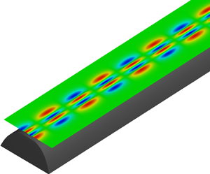
For a tsunami originated at the top of ridge, Class I trapped waves, i.e. symmetrical wave patterns, are expected to be created, following symmetrical wave excitation. Due to the gravity effect, the disturbed water surface, i.e. the Gaussian bump, slumps and generates a series of radiating waves propagating outwards. Snapshots of the free surface patterns for A 0 = 3.0 m and σ = 3000.0 at different output times are shown in figure 9. Almost all of waves generated at the origin are evidently trapped by and propagate along the ridge. Following a few small waves propagating at the front, a strong group consisting of several big waves (referred to as ‘significant waves’, hereafter) can be clearly observed, which is followed by weaker tail oscillations. The strongest wave (with the biggest amplitude) is formed after several weaker waves at the front and then the amplitudes of the following waves gradually decrease towards the rear. Due to the dispersion effects, the total extent of the wave train stretches and the wave amplitudes decay as the propagation distance increases.
FUNWAVE predicted snapshots of free surface elevation for a tsunami generated on the ridge top at different output times, where the green and black dash lines respectively indicate the central line and boundaries of the ridge.

Predicted respectively by the Boussinesq model and the shallow-water model components in FUNWAVE-TVD, the time histories of surface elevation recorded at the ten stations (from A1 to J1) along the ridge top are shown in figure 10. The waves travelling at the front are relatively small, followed by the significant waves with much larger magnitudes and then the tails. These waves are in an unsteady state and the wave forms are similar to a group of dispersive waves. In the near field, the amplitudes of the waves at the front of the envelope are small; arriving sometime later is the wave with the highest peak. Towards the rear, the amplitudes of the waves gradually decrease. As each of the waves in the group travels at its own speed, the entire train of the trapped waves spreads out in the space. In addition to the first significant wave envelope appearing behind the small-amplitude oscillations travelling at the front, further major wave envelopes may emerge during the propagation process.
Time series of surface elevation recorded at the 10 stations along the ridge top, where the black solid lines and the red dotted lines respectively represent the predictions from the Boussinesq model and the shallow-water model in FUNWAVE-TVD.

The corresponding wavelet amplitude spectra for the free surface elevations recorded at the ten ridge-top stations are shown in figure 11. The waves travelling at the front are too small to be easily identified in the wavelet spectra. High-frequency wave components become prominent in the trains of significant trapped waves. Different wave components arrive at station A1 almost at the same time as it is near to the origin. However, in the stations away from the origin, the wave component with the highest frequency of approximately f = 2.22 × 10⁻³ Hz in the significant trapped wave group is found to arrive first while the components of lower frequency arrive later accordingly. This may be due to the fact that the velocities of higher-frequency waves are faster than those of the lower-frequency waves according to the new trapped wave theory as presented in the previous sections. As the wave components of lower frequencies travel more slowly, the corresponding wavelet spectra present a decreasing trend of frequency against time. The wavelet spectra stretch out to incorporate the waves decaying during propagation. Overall, the energy of the trapped waves is mainly concentrated in the range [0.4 × 10⁻³ Hz, 2.5 × 10⁻³ Hz], and the energy density in the spectra decreases with increasing propagation distance. To confirm these are trapped waves, (2.40) is used to evaluate the arrival time of each of the mode 0 waves with different frequencies from the source, which is also plotted as black lines in figure 11. The maxima of the spectra are successfully traced out by the black lines, which shows that these waves are mainly the mode 0 trapped waves in Class I.
Wavelet amplitude spectra of the predicted surface elevations recorded at the ridge-top stations as shown in figure 10, where the black solid lines denote the arrival time of the Class I mode 0 trapped waves of different frequencies.

In order to examine the behaviour of these trapped waves in the cross-sectional direction, figure 12 presents the wave amplitude profiles for the first significant wave envelope, together with another envelope, at cross-sections y = 600 km, 1200 km, 1800 km, 2400 km and 3000 km. The strong waves in the first significant envelope are mainly mode 0 trapped waves of Class I, and their profiles may be approximately predicted by (2.29) with f = 2.22 × 10⁻³ Hz. Slight discrepancies between the simulated results and the analytical solutions are detected and may be due to the existence of higher-mode waves. To confirm this, the mode 0, 1 and 2 waves of f = 2.22 × 10⁻³ Hz (the magnitudes for the waves of different modes at different sections are listed in table 1) are superposed to derive improved amplitude profiles and much better agreement has been subsequently achieved. As the waves propagate for a longer distance, other envelopes emerge after the first significant wave train. These envelopes are also composed of mode-0 trapped waves, and their profiles can be well predicted by the proposed analytical solutions with f = 0.67 × 10⁻³ Hz.
Comparison between the amplitude profiles of the first significant wave envelope (left column) and another envelope (right column) predicted by FUNWAVE (solid circles), calculated by (2.29) for mode 0 (solid lines) and obtained by superposing the first three modes (dash lines). Since (2.29) cannot define the wave amplitude at the ridge top, the simulated amplitudes are treated as analytical solutions at this point.

Superposition of the first three modes for Class I trapped waves with f = 2.22 × 10⁻³ Hz, which is used to produce the improved wave amplitude profile in figure 12.

In order to further investigate whether the trapped waves are strictly restricted to propagate along the ridge, the wave energy at different cross-sections of the ridge is calculated. The free surface elevations recorded at the gauge stations are used to calculate wave heights. The total energy at a given point is estimated using the linear water wave theory, i.e.  $E = (1/8N)\sum\nolimits_{i = 1}^N {\rho gH_i^2}$, where N is the total number of waves. The results calculated at the gauge stations in each column are added up to provide the energy of trapped waves. As shown in figure 13, the energy of the trapped waves along the ridge maintains constant, and the slight fluctuation as observed may be due to the statistical error. This again verifies that most of waves generated at the source are trapped by the oceanic ridge, except for small energy leak-out. These trapped waves are strictly limited within the ridge, carry the trapped energy and travel forwards along the ridge.
Wave energy along the ridge calculated from the FUNWAVE results.

To further investigate the effects of dispersion and nonlinearity on the trapped waves, which have been neglected when deriving the new analytical solutions, the simulation is re-run using the linearized shallow-water model component of FUNWAVE-TVD (i.e. turning off the dispersive and nonlinear terms of the Boussinesq model). The surface elevations recorded at the 10 ridge-top gauge stations have also been plotted in figure 10 (the red dot lines). The results are almost identical to those produced by the Boussinesq model, indicating that frequency dispersion and nonlinear terms in the Boussinesq equations may be neglected in the simulation of trapped waves along ocean ridges. Moreover, as the periods of the trapped waves produced in the simulations are all greater than 450 s (f = 2.22 × 10⁻³ Hz) and the corresponding wavelengths are more than 20 times larger than the water depth even at the toe of the ridge, the shallow-water assumption is clearly satisfied, and the SWE can be effectively used to approximate the problem. This confirms that the new analytical solutions presented in this work are reasonable and accurate.
To investigate the effect of initial tsunami magnitude on the wave-trapping process, a further simulation is conducted on the same bathymetry. The initial bump is modified with A 0 = 10 m whilst other parameters are unchanged. The surface elevations recorded at the gauge stations exhibit similar oscillation patterns, compared with the previous results obtained with A 0 = 3.0 m, i.e. a much less severe event. The results are not displayed here to save space but verify that a tsunami with higher initial amplitude does not essentially affect the wave-trapping dynamics.
To further examine the effect of the ridge width on the resulting wave dynamics, the ocean ridge is widened to 70 km and a further simulation is conducted with other model settings remained the same. Figure 14 compares the surface elevations recorded at the 10 ridge-top stations with those obtained on the original bathymetric profile. On the wider ridge, the small-amplitude oscillations travelling at the front present similar but slightly more complex patterns. The first few significant envelopes largely overlap with those predicted on the original bathymetry. However, the discrepancy gradually becomes more evident for the waves towards the rear and more wave trains appear in the simulation results obtained on the wider ridge. This is the direct result of more wave energy being trapped by the wider ridge, which has been revealed by the ray-tracing analysis in § 3. When the waves spread out from the source after the tsunami is initiated, the refraction due to the varying water depth acts like the centripetal force to pull the waves back and trap them along the ridge. However, there are always escaping waves due to the finite refraction distance for a ridge of limited width. Comparing with the original narrower ridge, the wider ridge provides a longer distance for refraction to more effectively pull some of the leaking waves back onto the ridge. As these extra waves travel a longer path, they appear at the later stage of the wave trains, modify the trapped wave dynamics and extend the wave trains. The amplitude profiles of the first few significant wave envelopes and also the extra wave trains created by the widened ridge can be all well predicted by the analytical solutions.
Comparison of the surface elevations recorded at the 10 ridge-top stations, where the solid lines represent the results obtained for the original ridge of 60 km width and the dotted lines present the predictions over a wider ridge of 70 km width. The tsunamis are generated at the top of the ridge.

The effect of the ridge profile parameter on the trapped waves is also tested by running an extra simulation with λ = 0.000135. As expected, the results are similar to those from the previous simulations and therefore detailed presentation and discussion are omitted for simplicity. Briefly, similar trapped wave patterns are observed, i.e. almost all waves are restricted over the ridge as Class I trapped waves and their velocities as well as their amplitude profiles can be well predicted by the current analytical solutions. More wave energy is trapped by this steeper ridge compared with the original bathymetry. This may be linked to enhanced wave refraction over such a steep ridge.
4.2. Tsunamis generated at the mid-slope of the ridge
Tsunamis generated at the mid-slope of the ridge (x 0 = 15 km) are expected to create both symmetrical and anti-symmetrical trapped wave patterns as the result of asymmetrical excitation. Figure 15 presents the FUNWAVE simulation results at different output times, in terms of free surface patterns near to the source area for A 0 = 3 m and σ = 3000. The initial disturbance to the water surface generates a tsunami, which subsequently propagates along the ridge. The ridge topography creates a mechanism to enforce the disturbance swinging back and forth in the transverse direction whilst propagating forwards.
Snapshots of the free surface elevation patterns near to the source area predicted by FUNWAVE at different output times, where the green and black dash lines respectively denote the central and boundary lines of the ridge. The tsunami is generated at the mid-slope point of the ridge.

The generated waves are trapped and guided by the ridge, as clearly shown in figure 16. These trapped waves have their highest amplitudes for the first few significant waves, which then decrease towards the rear. As the trapped waves propagate forwards, the extents of the wave trains spread out as the wave amplitudes decrease. Unlike the symmetrical trapped wave patterns induced by the tsunami generated at the ridge top, the waves oscillate back and forth in the transverse direction around the ridge's central line, and the amplitude of oscillations decreases as the waves propagate further.
Snapshots of free surface elevation across the whole simulation domain at different output times, predicted by FUNWAVE for the tsunami generated at the mid-slope of the ridge.

The time histories of surface elevation recorded at the 10-gauge stations along x = 2.4 km (from A2 to J2) are shown in figure 17. The temporal variation of water surface elevations presents more complicated oscillation patterns than those induced by the tsunami generated at the ridge top. The highest amplitudes are seen in the first few significant waves, followed by gradually decreasing wave amplitudes at the rear. No evident and complete wave envelope is detected in these temporal surface elevation profiles and the entire wave train spreads out during the propagation.
FUNWAVE predicted surface elevations at the 10 stations along x = 2.4 km for the tsunami generated at the mid-slope of the ridge.

Figure 18 plots the corresponding wavelet amplitude spectra. The energy of the trapped waves displays a wider frequency range. In the first significant wave train, both modes 0 and 1 of the Class I and modes 1 and 2 of the Class II trapped waves are present. This is confirmed by the coincidence between the arrival times predicted by (2.40) and (2.55) and the maxima of the spectra. High-frequency waves arrive earlier and also decay more quickly, and at the end, only mode 0 components of the Class I trapped waves exist.
Wavelet amplitude spectra corresponding to the surface elevations as shown in figure 17, where the black solid and dash lines respectively denote the arrival time of each frequency in the modes 0 and 1 of the Class I trapped waves, while the pink solid and dash lines depict the arrival time of each frequency in the modes 1 and 2 of the Class II trapped waves.

Figure 19 demonstrates the wave amplitude profiles in the cross-sectional direction for the biggest waves and the smaller waves in the later stage. The amplitude profiles for the biggest waves are neither symmetrical nor anti-symmetrical and vary in different sections. As revealed by the wavelet spectra, these significant waves include components of different modes for Class I and II trapped waves simultaneously, and their profiles can be accurately approximated by superposing the modes 0 and 1 of the Class I and modes 1 and 2 of Class II trapped waves (the magnitudes for each of the modes at different sections are listed in table 2). The amplitude profiles for those waves appearing in the later stage are symmetrical to the central line of the ridge and always above the still water level. According to the wavelet spectra, the waves in the later stage are mainly mode 0 of the Class I trapped waves and their profiles can be well predicted by the proposed analytical solutions at f = 0.78 × 10⁻³ Hz.
Comparison between the amplitude profiles of the biggest waves and the smaller waves in the later stage (right column) produced respectively by FUNWAVE (solid circles), mode 0 of Class I waves (solid lines) and the superposition of the first two modes of Class I and II waves (dash lines).

Superposition of the first two modes for Class I and II trapped waves respectively to predict the wave amplitude profiles as shown in the first column of figure 19.

The wave energy at different cross-sections is also calculated using the same approach, as explained in the previous subsection. The wave energy is again maintained at a nearly constant level across the domain, confirming that tsunami waves can be strictly trapped by the ridge. The effects of the ridge profile parameter and width on the trapped wave dynamics are also further analysed. Similar to the results obtained for the trapped waves excited at the top of the ridge, there is more energy trapped by the ridges with modified cross-sectional profiles for both Class I and II waves. Detailed results are omitted here to avoid repetition.
Finally, the trapped waves induced by the tsunami generated at the toe of the ridge are also simulated but the results are not presented here for detailed discussion. The results are similar to those generated by the disturbance originating at the mid-slope and present both symmetrical trapped wave patterns (Class I) and also anti-symmetrical patterns (Class II). As there is more energy leaking out from the domain, the oscillating waves over the ridge are smaller than those induced by the tsunamis generated at the top and mid-slope locations.
5. Conclusions
It has been increasingly recognized that oceanic ridges can guide tsunami propagation and cause delayed arrival of waves with larger amplitudes. In order to better explain such phenomena and describe the resulting wave characteristics, analytical solutions for the trapped waves over an oceanic ridge with a hyperbolic-cosine squared profile are derived from the linear SWE. In the new analytical solutions, the dynamically varying free surface of the trapped waves is described using the combination of the first and second kinds of the associated Legendre functions of degree ν and order u. The new complete solutions indicate that both symmetrical and anti-symmetrical trapped waves exist over a ridge of symmetrical topographical profile, which are denoted as Class I and II trapped waves.
The present solutions are derived from the linear SWE that do not consider frequency dispersion. However, the deduced dispersion relationships exhibit that trapped waves of different frequencies/modes propagate at different speeds. These dispersion relationships, arising from the existence of an uneven bed topography, can be formulated as algebraic equations, allowing explicit quantification of their sensitivity to the topographic profile. Only a finite number of wave modes can exist for a given ridge and wave frequency. Furthermore, a threshold exists so that only those trapped waves with frequencies higher than the threshold value can sustain on the ridge. In contrast to trapped waves over a triangular ridge, the group velocity of the trapped waves on the ridge of the adopted profile increases with increasing frequency/wavenumber. This is a surprising finding and contrary to the common perception of the behaviour of the group velocity reported in the literature. Possible explanation may be that trapped waves are generated due to the existence of an uneven bed topography and its kinetic properties are highly dependent on the ridge profile.
A ray-tracing method is also used to interpret the behaviours of trapped waves to provide more comprehensive physical insights. Snell's law is used to derive the analytical solution of the ray path of a wave propagating over the ridge under consideration. The trapped wave rays are a group of curves with the same nodes. If the ridge is sufficiently wide, all waves originating from the ridge top with the propagation angle of α ≠  ${\rm \pi}$/2 or 3 ${\rm \pi}$/2 are constrained to the caustic lines due to refraction.
Numerical experiments have been further conducted using the extensively validated FUNWAVE-TVD Boussinesq model to further confirm the validity of the analytical solutions. Representative tsunami waves are generated as an initial Gaussian bump centred respectively at the top, mid-slope and toe of the ridge. The simulation results indicate that the tsunami generated at the ridge top induces only symmetrical trapped waves while the trapped waves excited by the tsunamis generated at the mid-slope location and toe present both symmetrical and anti-symmetrical modes. The arrival times of the waves associated with all different frequencies and the cross-sectional wave amplitude profiles predicted by the numerical model can all be successfully produced by present solutions.
The current analytical solutions are derived based on the linear water wave theory, the effect of nonlinearity on trapped waves will be further investigated in the future. Following the previous studies of edge waves on an infinite beach (Eckart Reference Eckart1951; Ursell Reference Ursell1952), the present study is focused on trapped waves over an infinite ridge. The new analytical formulation is validated and confirmed for tsunami-inducing trapped waves. However, there also exist cases where waves have longer wavelengths than tsunamis (such as inertia–gravity waves) or propagate over a smaller ridge, which can potentially lead to more energy leakage. The present solutions can be readily extended to describe these scenarios following the approaches as proposed in the previous studies (Buchwald Reference Buchwald1968; Shaw & Neu Reference Shaw and Neu1981). Future work may also include investigation of wave-trapping mechanisms induced by tsunamis and other regular or random waves propagating to the ridge from a faraway location.
Acknowledgement
The authors thank the anonymous reviewers for their constructive comments and suggestions.
Funding
This research was supported by the National Key Research and Development Program of China [No: 2017YFC1404205], the National Natural Science Foundation of China [No: 52071128 and 51579090] and the Fundamental Research Funds for the Central Universities [No: 2019B12214].
Declaration of interests
The authors report no conflict of interest.


 Open access