


1. Introduction
1.1. Context and motivation
Breakage of dispersed liquid drops in a carrier flow is of importance in engineering, from industrial manufacturing of petrochemicals, polymers or pharmaceuticals, to transport of mixtures of oil, water and gas in pipelines (Galinat et al. Reference Galinat, Masbernat, Guiraud, Dalmazzone and Noı2005), in the environment with oil-spill mitigation strategies (Li et al. Reference Li, Miller, Wang, Koley and Katz2017); while gas bubbles breaking in turbulence controls mass exchange at the air–water interface, from lakes to the ocean (Deike Reference Deike2022). Quantifying mass exchange in such flows requires a model for drop break-up in turbulence over a wide range of parameters. Drops that disperse in a turbulent carrier flow typically lead to a distribution of drop diameters from  $\mathrm {\mu }$m to cm for oil-in-water problems.
In homogeneous turbulence, the transient evolution of the drop-size distribution is described by a population balance equation, whose source terms account for a set of physical phenomena, in particular, the rate of consumption of drops due to break-up, and the rate of production of drops due to the break-up of larger drops (Martinez-Bazan et al. Reference Martinez-Bazan, Rodriguez-Rodriguez, Deane, Montañes and Lasheras2010; Qi, Masuk & Ni Reference Qi, Masuk and Ni2020). The break-up kernel then determines the rate of production of drops, from one size to another, and can be decomposed into a parent break-up frequency and child-size distribution (Martinez-Bazan et al. Reference Martinez-Bazan, Rodriguez-Rodriguez, Deane, Montañes and Lasheras2010; Aiyer et al. Reference Aiyer, Yang, Chamecki and Meneveau2019; Gaylo, Hendrickson & Yue Reference Gaylo, Hendrickson and Yue2021; Ruth et al. Reference Ruth, Aiyer, Rivière, Perrard and Deike2022). A large variety of break-up mechanisms have been introduced (Balachandar & Eaton Reference Balachandar and Eaton2010), with most models for droplet break-up in a turbulent flow considering a single mechanism with drop interaction with a single turbulent eddy, or a continuum of turbulence scales, with fluctuations at the size of the drop being the most effective part of the process (Hinze Reference Hinze1955; Luo & Svendsen Reference Luo and Svendsen1996; Liao & Lucas Reference Liao and Lucas2009; Lalanne, Masbernat & Risso Reference Lalanne, Masbernat and Risso2019). Binary break-up is often assumed, while highly viscous or energetic break-up presents a rapid sequence with multiple time scales and processes (Roccon et al. Reference Roccon, De Paoli, Zonta and Soldati2017; Rivière et al. Reference Rivière, Ruth, Mostert, Deike and Perrard2022; Ruth et al. Reference Ruth, Aiyer, Rivière, Perrard and Deike2022). Several models consider dimensional units (Martinez-Bazan et al. Reference Martinez-Bazan, Rodriguez-Rodriguez, Deane, Montañes and Lasheras2010; Qi et al. Reference Qi, Masuk and Ni2020), complicating the comparisons between different configurations and missing some hidden controlling parameters, while empirical formula, with important assumptions in the models not rigorously verified, have been applied outside their initial fitting range (Tsouris & Tavlarides Reference Tsouris and Tavlarides1994; Andersson & Andersson Reference Andersson and Andersson2006; Martinez-Bazan et al. Reference Martinez-Bazan, Rodriguez-Rodriguez, Deane, Montañes and Lasheras2010). Recent computational work has investigated various aspects of the break-up of drops in turbulent flow, including long bubble lifetime near critical conditions and limits of the Hinze-scale concept (Vela-Martín & Avila Reference Vela-Martín and Avila2022), the interaction of turbulence cascade and the break-up dynamics in steady-state turbulent emulsion configuration (Crialesi-Esposito et al. Reference Crialesi-Esposito, Rosti, Chibbaro and Brandt2022; Crialesi-Esposito, Chibbaro & Brandt Reference Crialesi-Esposito, Chibbaro and Brandt2023), while experimental work has discussed the role of small-scale eddies in bubble break-up (Qi et al. Reference Qi, Tan, Corbitt, Urbanik, Salibindla and Ni2022) or drop break-up in a von Kármán flow (Ravichandar et al. Reference Ravichandar, Vigil, Fox, Nachtigall, Daiss, Vonka and Olsen2022). Separately, atomization of jets has received considerable attention, with analysis of the subsequent instabilities controlling the scale selection, break-up and drop-size distribution (e.g. Eggers & Villermaux Reference Eggers and Villermaux2008; Villermaux Reference Villermaux2020) or analysis of the flow vortical structure (e.g. Zandian, Sirignano & Hussain Reference Zandian, Sirignano and Hussain2018).
At this stage, no universal formulation exists over a wide range of controlling non-dimensional numbers, comparing inertial, capillary and viscous effects, and spanning various viscosity ratios and turbulence intensities. When the viscosity ratio is significantly larger than one, surface tension is less important and the break-up process can take much longer than the turbulence time scales, with viscous breakage only occurring when the drop has been substantially stretched, similar to low- $Re$ break-up (Stone Reference Stone1994; Andersson & Andersson Reference Andersson and Andersson2006; Roccon et al. Reference Roccon, De Paoli, Zonta and Soldati2017). We aim to describe the occurrence of break-up, the break-up time and the number and child sizes, as a function of a set of well-chosen non-dimensional numbers defined as a function of the liquids properties.
1.2. Non-dimensional numbers
Considering an initially spherical drop of diameter  $d$, viscosity $\mu _d$, and density $\rho _d$ in a turbulent carrier flow, characterized by velocity $U$, density $\rho _l$, viscosity $\mu _l$ and surface tension $\sigma$, we have seven controlling parameters, with three units, leading to four non-dimensional groups. Early theoretical discussion on drop break-up in turbulent flow (Hinze Reference Hinze1955) has mostly been based on the competition between inertial and surface forces, and as such the most important relevant dimensionless quantity is the Weber number
 \begin{equation} We = {\rho_d U^2 d}/{\sigma}={2\rho_d \varepsilon^{2/3}d^{5/3}}/{\sigma}, \end{equation}
where  $\varepsilon$ is the turbulence dissipation rate, used to characterize the inertial range of the turbulent flow. When considering a turbulent flow, the characteristic velocity is given by the root mean square fluctuations, $u_{rms}$, the energy-injection scale is the integral length scale, $L_{int}$, and the turbulence intensity is characterized by the turbulent dissipation rate, $\varepsilon$, with $\varepsilon = C_{\varepsilon }u_{rms}^3/L_{int}$ where $C_{\varepsilon } \approx 2$ is a non-dimensional number universal at high Reynolds number (Dimotakis Reference Dimotakis2005; Vassilicos Reference Vassilicos2015). The turbulence is characterized by the Reynolds number, which can be defined at the integral length scale: $Re = {u_{{rms}}L_{int}}/{\nu _l} \propto {k^2}/{\nu _l \varepsilon }$, with $\nu _l=\mu _l/\rho _l$ the kinematic viscosity and $k \propto u_{{rms}}^2$ the turbulent kinetic energy. Another commonly used characterization of the turbulent flow is the Taylor-scale Reynolds number, which compares the strength of velocity fluctuations within the inertial range
 \begin{equation} Re_{\lambda}= {u_{rms} \lambda}/{\nu_l}, \end{equation}
where  $\lambda$ is the Taylor microscale: $\lambda = \sqrt {{15\nu _l}/{\varepsilon }}u_{rms}=\sqrt {15\nu _l}({L_{int}}/{C_{\varepsilon }})^{1/3}\varepsilon ^{-1/6}$, such that $Re \propto Re_{\lambda }^2$. For $Re_{\lambda }>100$, the mixing properties become mostly independent of $Re$ (Dimotakis Reference Dimotakis2005; Mostert, Popinet & Deike Reference Mostert, Popinet and Deike2022).
For drops of low viscosity (or bubbles), break-up occurs above a certain critical Weber number,  $We_c^0$, which is of order one (Hinze Reference Hinze1955; Risso & Fabre Reference Risso and Fabre1998; Rivière et al. Reference Rivière, Ruth, Mostert, Deike and Perrard2022), and the associated Hinze scale can be defined: $d_h^0=({W e_c^0}/{2})^{3 / 5}({\sigma }/{\rho })^{3 / 5} \varepsilon ^{-2 / 5}$. As discussed in Rivière et al. (Reference Rivière, Mostert, Perrard and Deike2021, Reference Rivière, Ruth, Mostert, Deike and Perrard2022), the critical Weber number, or Hinze scale, should be considered as a soft limit as the turbulent flow presents large fluctuations, leading to a broad range of break-up times for the same turbulent conditions, especially close to stable conditions (Vela-Martín & Avila Reference Vela-Martín and Avila2022), which makes estimations of the critical Weber number challenging. For bubbles and low viscosity drops, variations in the experimentally reported values of the critical Weber typically go from 0.5 to 5 (Risso & Fabre Reference Risso and Fabre1998; Andersson & Andersson Reference Andersson and Andersson2006; Liao & Lucas Reference Liao and Lucas2009; Martinez-Bazan et al. Reference Martinez-Bazan, Rodriguez-Rodriguez, Deane, Montañes and Lasheras2010; Vejražka, Zedníková & Stanovskỳ Reference Vejražka, Zedníková and Stanovskỳ2018). The critical Weber number, or Hinze scale, is defined in a statistical sense, for a given time (and window) of observation, typically corresponding to the conditions where half of the droplets will break. Such a definition inherently depends on an observation time constrained by experimental or computational constraints. The range of critical Weber numbers observed can be related to variability in the experimental configurations with different large-scale shear or spatial variations of the dissipation rate.
When the viscosity of the liquid is increased, viscous effects will come into play and we introduce a dimensionless ‘viscosity group’ (Hinze Reference Hinze1955), which can be defined as the Ohnesorge number:  $Oh = {\mu _d}/{\sqrt {\rho _d \sigma d}}$. At low $Oh$ (typically $Oh <0.1$), viscous effects are not needed to describe break-up properties, while they become essential at higher $Oh$. This dimensionless viscosity group can be replaced by another choice of non-dimensional number, such as the viscosity ratio
 \begin{equation} \mu_r={\mu_d}/{\mu_l}. \end{equation}
Finally, the fourth non-dimensional parameter can be chosen as the density ratio, which is taken to be unity in the present study,  $\rho _d/\rho _l \approx 1$, relevant for several oil-in-water problems.
The paper is organized as follows: § 2 presents the computational approach and the large ensemble of simulations performed. Section 3 discusses the critical break-up conditions as a function of the appropriate viscosity group, and characterizes the associated time scale of break-up and size distribution of drops. Section 4 presents conclusions and perspectives for future work.
2. Approach
We perform direct numerical simulations (DNS) of the two-phase, incompressible Navier–Stokes equations with surface tension using the open-source software Basilisk (Popinet Reference Popinet2015, Reference Popinet2018). We solve the full two-phase Navier–Stokes equations based on a quad/octree adaptive spatial discretization and a multilevel Poisson solver. The interface between the two liquids is reconstructed by a sharp geometric volume-of-fluid (VOF) method, momentum-conserving scheme and an accurate, well-balanced surface tension model. The methodology has been demonstrated to be accurate for capturing the multi-scale nature of turbulent multiphase flows involving break-up, leveraging adaptive mesh refinement, where the spatial discretization is adjusted to follow the spatial and temporal evolution of flow structures. This has been amply demonstrated in recent work on breaking waves (Deike, Melville & Popinet Reference Deike, Melville and Popinet2016; Mostert & Deike Reference Mostert and Deike2020; Mostert et al. Reference Mostert, Popinet and Deike2022), bubble bursting (Berny et al. Reference Berny, Deike, Séon and Popinet2020), bubble deformation and break-up in turbulence (Perrard et al. Reference Perrard, Rivière, Mostert and Deike2021; Rivière et al. Reference Rivière, Mostert, Perrard and Deike2021, Reference Rivière, Ruth, Mostert, Deike and Perrard2022) and bubble gas transfer (Farsoiya, Popinet & Deike Reference Farsoiya, Popinet and Deike2021; Farsoiya et al. Reference Farsoiya, Magdelaine, Antkowiak, Popinet and Deike2023).
The simulations are performed in two steps. First, we perform a precursor simulation to generate a homogeneous, isotropic turbulent flow in a single phase, with well-defined properties. Second, we insert the drop with initially no velocity and analyse its evolution in the forced turbulent flow.
The turbulent flow is generated by a volumetric force that is locally proportional to the velocity at every point of the physical space. This approach has been introduced by Rosales & Meneveau (Reference Rosales and Meneveau2005) and produces a well-characterized, homogeneous, isotropic turbulent flow with properties that closely resemble those obtained with a spectral code. This approach has been used to study bubble rising (Loisy & Naso Reference Loisy and Naso2017), bubble deformation (Perrard et al. Reference Perrard, Rivière, Mostert and Deike2021), gas exchange (Farsoiya et al. Reference Farsoiya, Popinet and Deike2021, Reference Farsoiya, Magdelaine, Antkowiak, Popinet and Deike2023) and break-up (Rivière et al. Reference Rivière, Mostert, Perrard and Deike2021) in turbulence. The turbulence statistics, including kinetic energy, dissipation rate and turbulent Reynolds number  $Re_{\lambda }$ as a function of time, have been verified to reach a statistically stationary regime, while the second-order structure functions display a well-defined inertial range, in good agreement with the homogeneous, isotropic turbulence scaling described in the literature; as demonstrated in Perrard et al. (Reference Perrard, Rivière, Mostert and Deike2021), Rivière et al. (Reference Rivière, Mostert, Perrard and Deike2021) and Farsoiya et al. (Reference Farsoiya, Popinet and Deike2021, Reference Farsoiya, Magdelaine, Antkowiak, Popinet and Deike2023). Once the statistically stationary regime is reached, we extract the velocity fields at different times, termed as precursors, and utilize them as initial conditions for subsequent simulations where we introduce a drop in the central region. A central drop of diameter $d$ and density $\rho _d$ is placed in the domain, and the flow in the inner phase is initially set to be zero. The solver relaxes within a few time steps after the initialization and the velocity and pressure become unaffected by the specific initialization details well before deformations become significant. Each precursor is spaced by at least one eddy-turnover time at the scale of the drop to ensure statistical independence between the precursor flow. A detailed description of the numerical configuration can be found in Perrard et al. (Reference Perrard, Rivière, Mostert and Deike2021), Rivière et al. (Reference Rivière, Mostert, Perrard and Deike2021) and Farsoiya et al. (Reference Farsoiya, Popinet and Deike2021, Reference Farsoiya, Magdelaine, Antkowiak, Popinet and Deike2023).
The maximum level of refinement,  $L$, sets the smallest grid size in the domain and allows us to compare with a fixed grid, equivalent to $(2^{L})^3$ number of grid points. Adaptive mesh refinement allows us to reach a wide separation of scales and obtain grid convergence for child-size data. In the simulations in this study, the flow variables of interest are the VOF and velocity fields, as in Rivière et al. (Reference Rivière, Mostert, Perrard and Deike2021) and Mostert et al. (Reference Mostert, Popinet and Deike2022), and a full discussion on the adaptive mesh refinement algorithm can be found in van Hooft et al. (Reference van Hooft, Popinet, van Heerwaarden, van der Linden, de Roode and van de Wiel2018) and Mostert et al. (Reference Mostert, Popinet and Deike2022). Grid convergence is verified in multiple ways. First, the present numerical set-up is inherited from our work on bubble break-up, where grid convergence on break-up time, number of children and size distribution was verified for a wide range of Weber numbers (Rivière et al. Reference Rivière, Mostert, Perrard and Deike2021). Similarly, all metrics discussed in the present paper (break-up occurrence, time and size distribution of child droplets) are verified to be grid independent in an ensemble average sense, while individual realizations also demonstrate grid convergence (see Appendix A). Adaptive mesh refinement allows us to reduce the number of grid points, reducing memory requirements and run time and allowing us to perform a wide sweep of parameters at moderate cost. The typical number of grid points for L10 is between $3\times 10^6$ and $6\times 10^6$ depending on the values of $We$ and viscosity ratios (to be compared with $(2^{10})^3\approx 10^9$ grid points with a fixed grid, i.e. an ${\approx }200$-fold reduction in the number of grid points). Reaching a higher Reynolds number is feasible but significantly increases the number of grid points to resolve the finer scales of the turbulent flow, hence the computational cost increases. Here, we focus on the wide sweep in viscosity ratio and Weber number.
The ratio of the initial drop radius to the box size is 0.067 so that the volume ratio is 0.0012; and we can consider that we are in dilute regime. The drop size compared with the box size is not varied in the present work, and the drop is always in the inertial range (with slight variations of the ratio of the initial drop size with the turbulence length scales as the Reynolds number is changed; see Farsoiya et al. (Reference Farsoiya, Popinet and Deike2021, Reference Farsoiya, Magdelaine, Antkowiak, Popinet and Deike2023)). Because we are in the dilute regime, coalescence will be negligible statistically.
A wide range of parameters relevant to the physical problem is swept (see table 1), with  $\mu _r$ between $10^{-2}$ and 350, equivalent to $Oh$ from $10^{-5}$ to 28, in order to assess the role of viscosity in break-up frequency, child-size distribution and break-up morphology. The value of $We$ is varied from 1 to 30, spanning regimes including no break-up, break-up threshold and violent break-up. For each condition, we perform an ensemble of simulations (10 to 100 realizations) in order to obtain statistical convergence to the metrics of interest, following the approach successfully employed for bubble break-up (Perrard et al. Reference Perrard, Rivière, Mostert and Deike2021; Rivière et al. Reference Rivière, Mostert, Perrard and Deike2021, Reference Rivière, Ruth, Mostert, Deike and Perrard2022). Thanks to the adaptive mesh refinement approach, each individual run has a low computational cost making the very large ensemble possible.
List of simulations for various  $We$,
$We$,  $Re$ and $\mu _r$ indicating the level of resolution on the interface, the number of runs and the initial drop-to-grid-size ratio. The minimal length of the simulation is $t/t_c = 20$ for cases that do not break, where $t_c$ is the eddy-turnover time at the scale of drop diameter and is given by $t_c=d^{2/3}\varepsilon ^{-1/3}$. The simulation time is large compared with the Kolmogorov time scale $\tau _{\eta }$ with $t/\tau _{\eta } \approx 200$, where $\tau _{\eta }=\sqrt {\nu _l/\epsilon }$. Small ensembles are used to obtain the break-up phase diagram (figures 2 and 3), while large ensembles are used to obtain the child numbers and size distributions (figure 4).

We will define the critical Weber as in Perrard et al. (Reference Perrard, Rivière, Mostert and Deike2021) and Rivière et al. (Reference Rivière, Mostert, Perrard and Deike2021) in terms of the size of our ensembles (ranging from 10 to 150 runs per conditions) and the duration chosen for the simulations (at least 20 eddy-turnover times at the scale of the drop, equivalent to approximately 200 times the Kolmogorov time scale, which is long enough to capture significant statistical variability in the break-up time but is still manageable in terms of computational cost for the large range of parameters we consider) and explore the dependence of the obtained critical Weber number on the viscosity ratio and turbulence Reynolds number. We expect the proposed scalings for the mean lifetime to be independent of the definition while an analysis of the lifetime distribution would be sensitive to the statistical definitions (as in any other studies) used for the critical conditions. We note that all results presented here are statistically converged in terms of the size of the sample (i.e. results do not change if we only consider half of the ensemble per condition).
3. Drop break-up: occurrence, morphology and time
3.1. Drop morphology
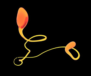
Examples of drop break-up in turbulent flow for increasing Weber number and viscosity ratios are shown in figure 1 and illustrate the complexity of the processes at play. The top row shows a low viscosity drop ( $\mu _r=0.01$) close to critical break-up conditions ( $We=4\gtrsim We_c^0$), with a mild break-up occurring on a time scale controlled by the turbulent flow, and leading to two children of similar sizes. The second row shows the effect of increasing the droplet viscosity, for the same turbulent flow and $We=4\gtrsim We_c^0$. As the viscosity of the drop increases, break-up is delayed and the formation of a thin thread prior to break-up is observed. This leads to an increased number of children with increasing $\mu _r$. Note that when further increasing the viscosity ratio at $We=4$, no break-up is observed within the observation time ( $t/t_c=20$).
Break-up event and drop morphology for  $Re_{\lambda }=77$, $We = 4$, $\mu _r = 0.01,10$ (a–f), $Re_{\lambda }=77$, $We=8$, $\mu _r = 0.01,150$ (g–l) and $Re_{\lambda }=77$, $We=20$, $\mu _r = 150$ (m–o). Hinze scale $d_h$ is shown, considering a constant $We_c^0$, and indicates the scale of the images. The time $t/t_c$ corresponds to the time since injection of the drop in the turbulent flow. The colour variation is due to the ray tracing of the oil droplet.

The next two rows show the  $We=8$ dynamics for increasing viscosity ratios. For low to intermediate viscosity ratios, a scenario somewhat similar to bag break-up is observed, reminiscent of the role of turbulent fluctuations at the drop scale at high $We$ far from critical conditions ( $We\gg We_c$). At very high viscosity ( $\mu _r=150$) and $We=8$, which is close to break-up threshold, we observe a very thin thread that characterizes the break-up, with a break-up time more than an order of magnitude longer due to the viscous effects. Finally, at $\mu _r=150$ and further from break-up threshold ( $We=20$, last row), the break-up happens faster but also leads to a very thin filament leading to many tiny drops. It is clear from these examples that the surrounding flow leading to break-up is different, with high stretching being required to create the elongated structure necessary for break-up with a possible importance of the internal flow of the drop.
3.2. Critical Weber number
We analyse the break-up threshold as a function of the various non-dimensional numbers. Figure 2(a) shows the break-up probability obtained from ensembles of simulations at various  $We$ and $\mu _r$, for $Re_{\lambda }=77$. Each point corresponds to an ensemble of ten runs with various precursors, and the condition is considered in the break-up region if more than 50 % of the cases broke before 20 $t_c$ after insertion. The critical $We$ ( $We_c$) is obtained from the contours of the break-up probability and is shown as a solid line, showing that $We_c$ is a function of $\mu _r$ for large viscosity ratio, at a given $Re$. Grid resolution is verified by running the same ensemble with higher refinement level. The simulation length of 20 $t_c$ was chosen as a trade-off between a long enough sequence to properly define the break-up occurrence and a reasonable computational cost to perform large ensembles for a wide range of conditions. This time corresponds to 200 $\tau _\eta$, the Kolmogorov time scale, so that the time we systematically explore is much longer than the times tested in Håkansson & Brandt (Reference Håkansson and Brandt2022), giving strong confidence in the resolution of the break-up boundaries. Note that the time for pinching is smaller than the eddy-turnover time, so when no break-up is observed at high viscosity ratio, it is not due to an incomplete pinching but simply because the conditions leading to break-up have not been met. As summarized in table 1, we performed close to 10 000 individual simulations at relatively high resolutions (interface resolution equivalent to $512^3$ to $1024^3$ grid points), systematically exploring high viscosity ratios, which is the focus on the study, and not the study of rare events, which would require a much larger number of eddy-turnover times.
Drop break-up phase diagram, as a function of  $We$ and viscosity group: $Oh$ (b); $\mu _r$ (c); and inverse of a drop Reynolds number (d). (a) Example of data analysis leading to extraction of the critical- $We_c$ line for $Re_{\lambda }=77$ and ${\rm \Delta} x/d_0=64$ (L9). Each symbol is for an ensemble of simulations obtained using different precursors, and the percentage of cases broken up within $20 t_c$ is colour-coded. The critical- $We_c$ line is extracted as the 50 % contour. (b) Critical- $We_c$ contours for various resolutions (circles $d_0/{\rm \Delta} x=64$, L9; squares $d_0/{\rm \Delta} x=128$, L10; and crosses $d_0/{\rm \Delta} x=32$, L8) and increasing $Re_{\lambda }$. Grid convergence is observed between the various resolutions at a given $Re_{\lambda }$, as shown by the overlapping symbols. At low $Oh$ (typically $Oh < 0.1$), a constant $We_c$ is observed, close to 2.5. At high $Oh$ ( $Oh > 1$), $We_c$ becomes a function of $Oh$ and $Re_{\lambda }$. (c) (3.1) shown as dashed lines introduces a characteristic viscosity ratio $\mu _r^0$ above which viscosity controls the break-up, with $\mu _r^0\approx 1.5 Re_{\lambda }$ (inset). (d) Break-up boundaries $We_c$ can be rescaled by the inverse of a drop Reynolds number $(({\rho _l}/{\rho _d})({\rho _d u_{rms} \lambda }/{\mu _d}))$.

Figure 2(b) shows  $We_c$ contours as a function of $Oh$, with $Oh$ ranging from 0.01 to 10, and $We$ from 0.5 to 30. We observe that, at low $Oh$ (low viscosity), break-up occurs at $We$ close to $We_c\approx 2.5$, in agreement with values reported in the literature for low viscosity and bubble conditions (Rivière et al. Reference Rivière, Mostert, Perrard and Deike2021). At high $Oh$ (higher viscosity), we observe that $We_c$ is now a function of $\mu _r$. Additionally, higher $We$ needs to be reached to obtain break-up, and there is a weaker influence of the Reynolds number $Re_{\lambda }$. Here, $We_c$ is grid converged as shown in figure 2(b) by the different overlapping markers corresponding to increasing resolution.
Figure 2(c) shows  $We_c$ contours as a function $\mu _r$, for different $Re_{\lambda }$. We observe that $We_c$ is a function of $\mu _r$ alone, with the critical-Weber contour described by a constant value at low $\mu _r$, $We_c=We_c^0$, with $We_c^0\approx 2.5$, which can be seen as an absolute value at low viscosity. Note that the particular value might be slightly sensitive to the choice of averaging, i.e. the size of the ensemble, the 50 % threshold and duration of the simulations; here, 20 $t_c$ as for any statistical definition of critical break-up conditions in a turbulent flow. However, the critical value is within the bounds of the literature, and the important physical result is the existence of the critical value at low viscosity ratio; while when the viscosity ratio increases, $We_c$ becomes a steep function of $\mu _r$ for $\mu _r > 10$. Overall the data can be described by an empirical function
 \begin{equation} We_c = {We_c^0} \exp{\left({\mu_r}/{\mu_r^0}\right)}, \end{equation}
with the critical viscosity ratio  $\mu _r^0$ obtained for each $Re$ by a least-squares fit. In the present simulations, $\mu _r^0$ is found to scale linearly with $Re_{\lambda }$: $\mu _r^0 = 1.5 Re_{\lambda }$; see inset. A similar discussion could be provided using $Oh$. The transition from the inertial to the viscous regime can be interpreted as a constant drop viscosity Reynolds number, since $\mu _r^0 \approx 1.5 Re_{\lambda }$ is equivalent to $1/(({\rho _l}/{\rho _d})({\rho _d u_{rms} \lambda }/{\mu _d}))\approx 1.5$, so that (3.1) becomes
 \begin{equation} We_c = {We_c^0} \exp{\left(\frac{1}{1.5}\frac{\rho_l}{\rho_d}\frac{\rho_d u_{rms} \lambda}{\mu_d}\right)}, \end{equation}
which rescales all data onto a single curve, as shown in figure 2(d).
Note that the functional form in (3.1) is the simplest one we could find, with the smallest number of parameters, but is not justified by a physical argument at this point and that other functional forms could be applied. We also comment that we did not vary independently the density ratio when demonstrating the rescaling (3.2), and that the range of Reynolds numbers tested remains limited (with  $Re_\lambda$ from 40 to 80) due to the higher computational cost for higher Reynolds numbers. While the values of the Taylor-scale Reynolds number are modest, they are high enough to observe a reasonable inertial range, as shown in Perrard et al. (Reference Perrard, Rivière, Mostert and Deike2021), Rivière et al. (Reference Rivière, Ruth, Mostert, Deike and Perrard2022) and Farsoiya et al. (Reference Farsoiya, Popinet and Deike2021, Reference Farsoiya, Magdelaine, Antkowiak, Popinet and Deike2023) and correspond to integral-length-scale Reynolds number from 100 to 400 approximately (with a scaling between the integral-length-scale and Taylor-scale Reynolds numbers being $Re_{int}\propto Re_\lambda ^2$; see Pope Reference Pope2000).
We can then define a viscosity group–dependent Hinze scale  $d_h$ that separates stable drops ( $d< d_h$) from those that will break ( $d>d_h$) using the viscosity-dependent $We_c$ for the break-up $We_c(\mu _r)$: $d_h=({W e_c(\mu _r)}/{2})^{3 / 5}({\sigma }/{\rho })^{3 / 5} \varepsilon ^{-2 / 5}$.
3.3. Drop break-up frequency
Within the break-up regime shown in figure 2, we extract the (first) break-up time of the drop  $T$ for each realization that breaks and compute its ensemble average $\langle T \rangle$. Figure 3 shows the non-dimensional break-up frequency $t_c/\langle T\rangle$ as a function of $We$ for various $\mu _r$ at $Re_{\lambda }=77$. The break-up frequency increases with $We$ while reaching saturation values that increase from high to low $\mu _r$. The overall trend for each $\mu _r$ is similar to what has been observed for bubbles (Martinez-Bazan et al. Reference Martinez-Bazan, Rodriguez-Rodriguez, Deane, Montañes and Lasheras2010; Rivière et al. Reference Rivière, Mostert, Perrard and Deike2021). The data can be described by a formula based on energy arguments (Martinez-Bazan et al. Reference Martinez-Bazan, Rodriguez-Rodriguez, Deane, Montañes and Lasheras2010),
 \begin{equation} \frac{t_c}{\langle T\rangle } = \alpha(\mu_r) \sqrt{\frac{We}{We_c(\mu_r)}-1}, \end{equation}
where  $\alpha (\mu _r)$ is a parameter that is obtained by least-squares fitting of the data, while $We_c(\mu _r)$ is given by (3.1). All data can then be rescaled using the parameter $\alpha (\mu _r)$ as shown in figure 3(b) for a single $Re$. The same procedure is applied at each $Re$ (and resolution), and shown in figure 3(c), demonstrating grid convergence (symbols of increasing sizes correspond to increasing resolution and overlap). The values of $\alpha (\mu _r)$ (expressed in terms of the drop Reynolds number) are shown in figure 3(d), with a maximum value of 0.3 at low viscosity and decaying exponentially to reach a value of 0.1 at high viscosity.
(a) Ensemble-averaged drop first break-up frequency  $t_c/\langle T \rangle$ made dimensionless using the eddy-turnover time at the scale of the initial drop, for increasing $\mu _r$, at $Re_\lambda =77$ (and L9). Equation (3.3) is fitted to the data for each $\mu _r$ (dashed lines), defining $\alpha (\mu _r)$. (b) Same data showing the rescaled break-up frequency $t_c/\alpha (\mu _r)\langle T \rangle$ as a function of the distance to $We_c(\mu _r)$. (c) Data for L8 (small symbols), L9 (medium) and L10 (large) show grid convergence and various $Re$. All data collapse onto a single curve. (d) The value of $\alpha (\mu _r)$ is a function of $\mu _r$ and $Re_\lambda$, and decreases with the drop Reynolds number.

Note that, as discussed by Håkansson (Reference Håkansson2020), the use of a break-up frequency within a population model must be made in a consistent way. Here, our definition of the break-up frequency has no ambiguity in the region of the break-up diagram where all cases break before 20 $t_c$ (equivalent to 200 $\tau _\eta$, significantly larger than any of the break-up times discussed by Håkansson & Brandt Reference Håkansson and Brandt2022), which is almost all data points except the ones on the boundary (see figure 2). For the parameters close to the boundary, the mean break-up time can become close to the window of observation, and less than 100 % of the ensemble leads to break-up.
3.4. Droplet production and size distribution
We now discuss droplet production and size distribution as a function of distance to critical conditions (quantified by  $We/We_c(\mu _r)$) and viscosity ratio $\mu _r$.
Figure 4(a,b) shows the child-size distribution of the first break-up obtained from large ensembles ( $\approx$100 runs per condition), for $\mu _r=0.01,10,150$ and $We/We_c\approx 1.5$ and 3.2 (corresponding to $We=4$, 8 or 20 depending on $\mu _r$), close to critical conditions (a, $We/We_c\approx 1.5$) and far from critical conditions (b, $We/We_c\approx 3.2$).
Number and size of drops production. (a,b) Child-size distribution of the first break-up event for the six large ensembles (order 100 realizations). Volumes are normalized by the volume of the initial parent droplet. The symbols are DNS data (L10), while the solid (dashed) lines are the probability density function from L10 (L9) data estimated using a Gaussian kernel density estimate, close to (a) and far from (b) critical conditions. (c) Ensemble-averaged number of drops  $\langle N\rangle$ produced after the first break-up as a function of time, for the large ensembles, counting drops with more than 4 grid points per diameter at L9 (solid line L10, dashed line L9, showing reasonable grid convergence). (d) Number of drops $\langle N \rangle$ at $(t-{T})/t_c=2$ as a function of $We/We(\mu _r)$ for different viscosity ratios. Circles are from small ensembles (10 realizations) and squares are from L10 large ensembles. (e,f) Drop-size distribution for the large ensembles taken at $(t-T)/t_c=2$. Drops larger than $4 {\rm \Delta} x$ are grid converged, close to (e) and far from (f) critical conditions. The shape of the distribution presents large variations depending on distance to criticality and viscosity ratio.

For low to intermediate  $\mu _r$ ( $\mu _r=0.01,10$), at $We$, close to critical conditions (a) ( $We/We_c(\mu _r)\approx 1.5$), the child-size distribution presents an M shape, compatible with previous descriptions of drop or bubble break-up in turbulence close to critical conditions (e.g. Rivière et al. Reference Rivière, Mostert, Perrard and Deike2021), corresponding to the production of two children of volumes 0.7 $V_0$ and 0.3 $V_0$ as the most probable event. At high viscosity, here $\mu _r=150$, break-up at $We=4$ does not happen since $We_c(\mu _r=150)\approx 6.5$. When considering $\mu _r=150$ close to critical conditions ( $We/We_c(\mu _r)\approx 1.5$), the child-size distribution clearly changes compared with low viscosity break-up close to critical conditions, with the production of two identical volumes being the most probable outcome, illustrating the change in dynamical regime for the first break-up of viscous drops.
When increasing  $We$ moving away from critical conditions (b), $We/We_c(\mu _r)\approx 3.5$, at low viscosity ratio, we observe a transition to a U shape, again compatible with previous descriptions (Rivière et al. Reference Rivière, Mostert, Perrard and Deike2021; Ruth et al. Reference Ruth, Aiyer, Rivière, Perrard and Deike2022), with a very small and a very large drop being formed, with similar results for $\mu _r=0.01,10$. However, at a high viscosity ratio, the distribution is close to a bell shape (similar to the shape of the distribution at lower $We$ for the same viscosity ratio) corresponding to two lobes of equal size, just prior to the fragmentation into tiny droplets of the snake like shape seen in figure 1.
Models have been developed to rationalize the observed shape of the child-size distribution of a binary break-up. As summarized by Qi et al. (Reference Qi, Masuk and Ni2020) and Rivière et al. (Reference Rivière, Mostert, Perrard and Deike2021), models for the first break-up child-size distribution lie in three categories: bell shaped (Martínez-Bazán, Montanes & Lasheras Reference Martínez-Bazán, Montanes and Lasheras1999), U shaped (Tsouris & Tavlarides Reference Tsouris and Tavlarides1994; Luo & Svendsen Reference Luo and Svendsen1996) or M shaped. Bell-shaped models correspond to two equal drops as the most probable outcome, while very unequal break-up that creates a small and a large bubble has a high probability in U-shaped models. Finally, the M-shaped models postulate that there is an unequal break-up that is the most likely. The three models correspond to different assumed physics of the break-up. A mechanism proposed to explain the M-shape distribution is that eddies smaller or equal to the drop size collide with the initial drop, which then excite and break the drop in one eddy-turnover time (see Qi et al. Reference Qi, Masuk and Ni2020), while the idea of various eddies leading to oscillations at the drop or bubble resonance frequency has also been proposed (Risso & Fabre Reference Risso and Fabre1998). Using the M-shape in a population balance model would require physical configurations where the break-ups are independent from one another and always at moderate conditions (close to critical conditions). A mechanism proposed to explain the U-shape distribution can be based on minimizing the surface energy increment, where the difference between the total surface energy before and after break-up controls the probability and a smaller difference means a larger probability for such break-up to happen. The U-shape distributions can be seen as resulting from the tearing of a small part of the initial drop (or bubble) and can correspond to the beginning of a more complicated break-up sequence. The U-shape is therefore often used in population balance models, as it allows us to recreate a rapid sequence as long as the model for the successive break-up times is adequate (see Ruth et al. Reference Ruth, Aiyer, Rivière, Perrard and Deike2022). A discussion on the bell shape is provided by Martínez-Bazán et al. (Reference Martínez-Bazán, Montanes and Lasheras1999), and relates to the assumption that the probability of generating a child drop of a specific size is proportional to the product of the excess stress of the two children, where the excess stress is the difference between the turbulent dynamic pressure around the children and the capillary pressure of the parent.
To summarize, the first break-up child-size distribution of drops in turbulence is controlled by two parameters: the distance to critical conditions, with a transition from M-shape to U-shape at low viscosity ratio, and the viscosity ratio itself, with a bell shape both close and far from critical conditions.
However, we caution that the analysis of the first break-up child size only gives part of the story hinted at by the very different geometrical properties of the break-ups (see figure 1) and the significant history effect being present when considering longer time evolution and sequences of break-ups. Indeed, at high viscosity ratios, the first break-up is described by a bell shape, which misses the production of tiny drops related to the snake like geometry.
Figure 4(c) shows the number of drops being produced as a function of time after the first break-up for the same ensembles ( $t-T$) (each curve starts with 2 drops at $t-{T}=0$). Close to critical conditions ( $We/We_c\approx 1.5$), we observe a mild increase up to 3 to 4 drops, as very few break-up events occur, compatible with the classic Kolmogorov–Hinze cascade of drop break-up, producing children of similar sizes and the cascade ends at the Hinze scale.
Now considering a high viscosity ratio,  $\mu _r=150$, still close to critical conditions ( $We/We_c(\mu _r)\approx 1.5$, which is now $We=8$ instead of 4) we observe significantly more drops formed over the time period than for the low viscosity cases, with up to 10 drops produced, corresponding to the final break-up of elongated filaments, even close to critical conditions.
As we move away from critical conditions,  $We/We_c(\mu _r)=3.2$, for low to intermediate $\mu _r$, we observe a strong increase of the number of drops (similar to that reported for bubbles), with 15 to 20 drops at $(t-T)/t_c=2$ (with the number of drops increasing with increasing viscosity ratios). At large viscosity ratio and similar $We/We_c(\mu _r)=3.2$, we now observe more than 50 droplets related to the extreme stretching of the ligament before break-up.
The number of drops produced is therefore a function of both the distance to critical conditions and the viscosity ratio, with both parameters leading to an independent increase of the number of drops produced. This is confirmed by figure 4(d), which shows  $\langle N \rangle$ (taken at $(t-{T})/t_c=2$) as a function of $We/We_c(\mu _r)$. For $\mu _r$ up to 10, we observe a linear increase in the number of drops with $We/We_c(\mu _r)$, independent of the viscosity ratio. The break-up is inertial with no influence of viscosity, similar to the dynamics of bubble break-up described by Rivière et al. (Reference Rivière, Mostert, Perrard and Deike2021, Reference Rivière, Ruth, Mostert, Deike and Perrard2022). When the viscosity ratio is further increased, the number of drops increases much more sharply.
The drop-size distributions for the large ensembles are shown in figure 4(e,f), taken at  $(t-{T})/t_c=2$. After two eddy-turnover times of the initial drop, the effect of the complete break-up sequence can be discussed on the drop-size distribution, and the role of distance to criticality and viscosity ratio is further confirmed. The time evolution of the drop-size distribution is shown in Appendix B and confirm that analysis after 2 $t_c$ is robust and that we have large enough statistical sample to analyse the shape of the drop-size distribution.
At low  $\mu _r$ and $We/We_c(\mu _r)\approx 3$, we observe a distribution close to the $d^{-3/2}$ scaling, reminiscent of capillary processes driving fragmentation of large volumes (Rivière et al. Reference Rivière, Ruth, Mostert, Deike and Perrard2022; Ruth et al. Reference Ruth, Aiyer, Rivière, Perrard and Deike2022), with a shape that is not a direct result of the first break-up, as rapid break-ups follow the initial one, leading to a broad sub-Hinze population.
Close to critical conditions, at low viscosity ratios, we observe a size distribution coherent with the child-size distribution of the first break-up with mostly drops close to the Hinze scale. The behaviour of the highest  $\mu _r$ is quite different, with a large number of drops being produced, but their sizes are all concentrated at the smallest possible scale being resolved, i.e. the scale of the filament at break-up, which is a consequence of the very strong thinning visible in figure 1. Such a shape could not be inferred from the first break-up, which displays two lobes of similar sizes, as the thin filament has not yet broken into multiple small drops.
4. Conclusions
We performed large ensembles of DNS of drop break-up in isotropic turbulence, spanning orders of magnitude in  $\mu _r$ and $We$, while also exploring the sensitivity to $Re$. We report a break-up occurrence diagram, which confirms a constant $We_c$ for low $\mu _r$, while $We_c$ becomes a function of a drop Reynolds number combining $\mu _r$ and $Re$ when $\mu _r$ increases. The first break-up time is found to be a function of the distance to $We_c$, with an increased break-up time as drop viscosity increases. Finally, the drop production and size distribution are analysed. We demonstrate the limits of only looking at the first break-up as the break-up sequences over an extended period of time present very different statistical behaviour, with different dynamical regimes at low and high $\mu _r$, and depending on the distance to critical conditions. This confirms that population balance models for drops should include a multi-time-scale drop-size distribution to account for break-up sequences, especially at high $We$ and high drop Reynolds number. The present work paves the way for a detailed analysis of the break-up mechanisms, including the role of the flow surrounding the drop prior to break-up and the internal drop dynamics for the different regimes identified.
Acknowledgements
This work was supported BASF SE and by NSF grant 2242512 to L.D. Computations were performed on Quriosity, BASF SE supercomputer. We thank S. Popinet for scientific discussions and development of the Basilisk package. We thank the Center for Multiphase Flow Research and Education at Iowa State University for supporting this project.
Declaration of interests
The authors report no conflict of interest.
Appendix A. Grid convergence
Together with the statistical convergence shown in figures 3, 4 and 5 for the droplet occurrence, first break-up time and number of drops as a function of time, we show here the grid convergence between levels 9 and 10 for selected typical individual runs. Figure 5 shows the drop diameter as a function of time for representative examples of droplet diameter, using the same precursor and two different maximum levels of resolution, for distance to critical condition,  $We/We_c(\mu _r)\approx 1.3$ and 3.2 and viscosity ratios $\mu _r=0.01$, 10 and 150 (corresponding to $We=4$, 8 and 20 to match the distance to critical conditions). These cases are a subset from the large ensembles shown in figures 4 and 5. Time $0$ corresponds to the injection of the drop in the turbulent precursor. In all cases, we can see that the first break-up occurs at nearly the same times at both levels of resolution and produce a similar number of drops of nearly the same sizes for drops of sizes resolved with more than 4 to 8 grid points per diameter. This empirical convergence threshold is in agreement with the description from Rivière et al. (Reference Rivière, Mostert, Perrard and Deike2021) regarding bubble break-up. As the break-up sequence progresses, more drops are produced and the sequences remain very similar.
Drop-diameter trees: time evolution of the drop diameter throughout the break-up sequence, for a representative set of simulations, demonstrating grid convergence between L9 (black) and L10 (red). Overall, break-up time, number of children and their size are grid converged for the various cases, as long as drops are resolved with a least 4 to 8 grid points per diameter.

Appendix B. Time evolution of the drop-size distribution
Figure 6 shows the time evolution of the size distribution for three large ensembles shown previously in figure 4. Within the first 2 $t_c$ after the first break-up, the number of drops increases but the overall shape of the distribution remains similar for each case, justifying the discussion on the size distribution at 2 $t_c$ after break-up.
Time evolution of the drop-size distribution for the three representative large ensembles (Weber number and viscosity ratio indicated on the top of the panel) showing that the size distribution shape at  $(t-T)/t_c=2$ is representative of the break-up sequence.


 Open access