







1. Introduction
Rivers, estuaries and coastal oceans are some examples of free surface flow environments that often exhibit shallow depths (a few metres), moderately strong currents (up to a few metres per second) and fairly complex bottom topography. The free surface flow on which we particularly focus is the nearshore environment – the transition region between the shoreline and the open ocean (see figure 1a). The nearshore region horizontally stretches for approximately 1 km, and consists of the surf zone (region of wave breaking) and the inner shelf (depths varying from a few metres to tens of metres) (Lentz & Fewings Reference Lentz and Fewings2012; Kumar & Feddersen Reference Kumar and Feddersen2017). Cross-shelf transport, i.e. the exchange of sediments, pollutants, nutrients, larvae, and pathogens between the coastal waters and the open ocean, is arguably the central problem in coastal physical oceanography (Lentz et al. Reference Lentz, Fewings, Howd, Fredericks and Hathaway2008; Brink Reference Brink2016). Cross-shelf currents are much weaker than alongshore currents. In the surf zone, cross-shelf and alongshore currents can respectively reach up to  $0.2$ and $1.5\ {\rm m}\ {\rm s}^{-1}$ (Bakhtyar et al. Reference Bakhtyar, Dastgheib, Roelvink and Barry2016). In the inner shelf region, the cross-shelf current can typically have a magnitude of $0.01\unicode{x2013}0.1\ {\rm m}\ {\rm s}^{-1}$, whereas the corresponding alongshore current is $0.1\unicode{x2013}0.5\ {\rm m}\ {\rm s}^{-1}$ (Rao Reference Rao2004). However, cross-shelf gradients of most properties are usually far greater than those in the alongshore direction, which causes cross-shelf exchange to dominate the rates and pathways of tracer delivery and removal on the continental shelf (Brink Reference Brink2016). Onshore-propagating surface waves lead to cross-shelf transport in the onshore direction via the Stokes drift mechanism – net mass transport in the direction of surface wave propagation (Stokes Reference Stokes1847) – while Eulerian return flow and transient rip currents are some of the important mechanisms causing offshore transport (Lentz et al. Reference Lentz, Fewings, Howd, Fredericks and Hathaway2008; Brown et al. Reference Brown, MacMahan, Reniers and Thornton2015; Kumar & Feddersen Reference Kumar and Feddersen2017; O'Dea, Kumar & Haller Reference O'Dea, Kumar and Haller2021).
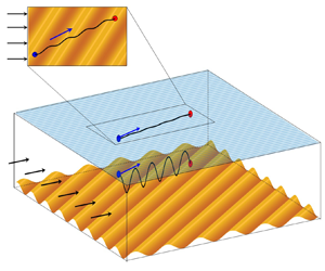
(a) A typical nearshore environment (location: Mallaig, Highlands of Scotland) and (b) the corresponding schematic diagram showing surface waves (wavenumber  $K(k,0)$), alongshore current ( $V_0$), wavy bottom topography (wavenumber $K_b(k_b,l_b$)) and the free surface imprint resulting from current–bathymetry interactions. Two subsets of the above situation are considered: (c) surface waves, flat bottom and alongshore current and (d) wavy bottom topography and alongshore current, but no surface waves. In the last case, the undulations at the free surface represent the surface imprint of the wavy seabed. The black dashed line is used for the shoreline, and the green dot in (a,b) represents a particle at the ocean surface.

The schematic in figure 1(b) provides an idealized representation of figure 1(a). This idealized scenario consists of three key elements: (i) a steady, uniform, alongshore current, (ii) onshore-propagating monochromatic surface waves and (iii) a small-amplitude, monochromatic bottom topography with wavevector making an oblique angle with the shoreline. Nearshore oblique sandbars have been observed in various locations, e.g. Trabucador Beach, Duck Beach, several Oregon beaches, St James Island, Durras Beach, etc. (Ribas, Falqués & Montoto Reference Ribas, Falqués and Montoto2003). According to our current understanding, the motion of a tracer parcel in the simplified set-up given in figure 1(b) is expected to result from two different mechanisms: Stokes drift and longshore drift (advection by the alongshore current). Hence we expect a tracer parcel to move in a resultant direction whose streamwise component is along  $+y$ (due to the longshore drift) and cross-stream component is along $+x$ (or onshore, due to the Stokes drift). The question we ask is – if we replace the set-up in figure 1(b) with a flat bathymetry (see figure 1c), does it alter the trajectory of a given tracer parcel? The primary objective of this paper is to show that small-amplitude wavy bottom topography indeed affects tracer trajectories, and in fact, can play a crucial role in cross-shelf (in a generic open-channel flow, this would imply cross-stream) tracer transport.
The fact that small-amplitude bottom topography can impact cross-shelf tracer transport is non-obvious. If we assume surface waves in figure 1(a) or 1(b) to be absent, basic fluid mechanics tells us that the tracer parcel marked by green dot will be simply advected in the  $+y$ direction by the alongshore current (i.e. undergo longshore drift). In the presence of small-amplitude topography, we show that an additional mechanism is at play, which can lead to cross-shelf (along $+x$ or $-x$) tracer transport. The proposed mechanism owes its existence to the stationary waves generated due to a uniform flow over a sinusoidal bottom topography (Thomson Reference Thomson1886; Lamb Reference Lamb1932). These stationary waves (or steady surface imprints of the sinusoidal wavy bottom) are shown in figure 1(d); they also exist in figure 1(b), and can be unravelled by removing the propagating surface waves entirely. The amplitude of these surface imprints may not be insignificant in fluvial and coastal environments owing to their shallow depths and high velocity scales, and hence can lead to non-trivial kinematics.
The outline of the paper is as follows. In § 2, we provide the general mathematical formulation of the problem. In § 3, we concentrate on figure 1(c) and onshore tracer transport of floating particles due to Stokes drift. Section 4 focuses on figure 1(d) and reveals a new drift mechanism resulting from the alongshore current and wavy seabed interactions. How this drift mechanism can contribute to the cross-shelf transport, and hence affect the fate of tracer parcels, is discussed in detail. In § 5, we discuss the set-up in figure 1(b), i.e. the combined effect of surface waves, wavy seabed and alongshore current. Section 6 provides a comparison of the Lagrangian transport due to Stokes drift, the new drift mechanism, and their combination for realistic parameters. The paper is summarized and concluded in § 7.
2. Mathematical formulation
We consider the three-dimensional problem of surface wave propagation over an undulating seabed in the presence of uniform background current (see figure 1b). We assume the fluid to be irrotational, incompressible, inviscid and homogeneous; the domain has infinite horizontal extent but has a finite mean depth  $H$. Surface tension and Coriolis effects are neglected. The water surface is denoted by $z=\eta (x,y,t)$; $x$ and $y$ respectively denote the cross-shelf (onshore and offshore are used respectively for positive and negative $x$ directions) and the alongshore (i.e. streamwise) directions, while the $z$-axis is directed upwards. The wavy seabed is denoted by $z=-H+\eta _b(x,y)$, where $|\eta _b/H| \ll 1$. We also consider a uniform cross-shelf current, $U_0$, and a uniform alongshore current, $V_0$. The fluid motion is defined by a velocity potential, which is a combination of the velocity potential due to the uniform currents, and the perturbed velocity potential ( $\phi$). The perturbed velocity potential satisfies the governing Laplace equation (GLE)
 \begin{equation} [\mathrm{{GLE}}]: \quad \phi_{,xx}+\phi_{,yy}+\phi_{,zz}=0, \quad {-H+\eta_b< z<\eta} , \end{equation}
where the comma subscript denotes partial derivative ( $\phi _{,x}=\partial \phi /\partial x$). Hereafter, unless specifically mentioned, velocity potential will always imply a perturbed quantity. The impenetrability condition (ImC) holds at the wavy seabed, $z=-H+\eta _b(x,y)$,
 \begin{equation} [\mathrm{ImC}]: \quad \phi_{,z}-\phi_{,x} \eta_{b,x}-\phi_{,y} \eta_{b,y}=U_0 \eta_{b,x}+V_0 \eta_{b,y}. \end{equation}
The ImC is a non-homogeneous equation in general, and would lead to a homogeneous solution only when the level sets of  $\eta _b$ are parallel to the background current field. The kinematic (KBC) and dynamic boundary conditions (DBC) at the free water surface, $z=\eta (x,y,t)$, are respectively given as
 \begin{gather} {}[\mathrm{KBC}]: \quad \eta_{,t}+(\phi_{,x}+U_0)\eta_{,x}+(\phi_{,y}+V_0)\eta_{,y}-\phi_{,z} =0, \end{gather}
 \begin{gather}{}[\mathrm{DBC}]: \quad \phi_{,t}+\tfrac{1}{2}[(\phi_{,x})^2+(\phi_{,y})^2+(\phi_{,z})^2]+U_0 \phi_{,x}+V_0 \phi_{,y}+g\eta =0, \end{gather}
where  $g$ denotes gravitational acceleration. In order to apply the boundary conditions, the velocity potentials at $z=-H+\eta _b$ and $z=\eta$ need to be respectively Taylor-expanded about $z=-H$ and $z=0$. Furthermore, throughout the paper we consider a wavy seabed of the form
 \begin{equation} \eta_b={a_b}\cos{(k_b x + l_b y)}, \end{equation}
where  $k_b$ and $l_b$ are respectively the wavenumbers in the $x$ and $y$ directions, $a_b$ is the amplitude and $K_b \equiv \sqrt {k_b^2+l_b^2}$.
Hereafter we assume  $U_0 \ll V_0$ (and further assume $U_0 \lesssim {O}(\epsilon ^2)$), since away from inlets or river mouths, cross-shelf flows are typically much weaker than alongshore flows (Gelfenbaum Reference Gelfenbaum2005). We also consider two (small) spatial scales: wave steepness, $\epsilon = K a \ll 1$ ( $K$ is surface wave's wavenumber and $a$ is its amplitude), and wavy seabed steepness, $\epsilon _b=K_b a_b \ll 1$, and expand the velocity potential ( $\phi$) and surface elevation ( $\eta$) as perturbation series in terms of $\epsilon$ and $\epsilon _b$. The velocity potential and surface elevation can then be expressed in terms of $\epsilon$ and $\epsilon _b$ as
 $$\begin{gather} \phi=\left[ \phi_u^{(1)}+ {O}(\epsilon^2) \right]+\left[\phi_s^{(1)}+ {O}(\epsilon_b^2)\right], \end{gather}$$
 $$\begin{gather}\eta=\left[\eta_u^{(1)}+{O}(\epsilon^2)\right]+\left[ \eta_s^{(1)}+ {O}(\epsilon_b^2)\right]. \end{gather}$$
Both  $\phi$ and $\eta$ are a combination of an unsteady solution, denoted by subscript ‘ $u$’, and a steady solution, denoted by subscript ‘ $s$’ (Kirby Reference Kirby1988; Fan et al. Reference Fan, Zheng, Tao and Liu2021). The quantities $\phi _u^{(1)}$ and $\eta _u^{(1)}$ are ${O}(\epsilon )$, while $\phi _s^{(1)}$ and $\eta _s^{(1)}$ are ${O}(\epsilon _b)$. The steady solution, arising from the interactions between the uniform current and sinusoidal bottom topography, manifests itself as stationary waves (Thomson Reference Thomson1886; Lamb Reference Lamb1932). Such spatially varying stationary features can also be viewed as ${O}(\epsilon _b)$ corrections to the leading-order uniform flow due to the wavy seabed topography. In (2.5a)–(2.5b), the relationship between $\epsilon$ and $\epsilon _b$ is not yet established, and hence they are separated by square brackets. In the following sections, we investigate different situations depending on the relationship between $\epsilon$ and $\epsilon _b$.
The velocity field can be straightforwardly obtained from the velocity potential:  $\boldsymbol {u}\equiv (u,v,w)=(\phi _{,x},\phi _{,y},\phi _{,z})$. Out of the three components, the velocity $u$ plays the most crucial role in the cross-shelf transport of particles. Figure 2 shows contour plots of $u$ at an arbitrary time in the $x$–
$x$– $z$ plane for different situations depending on the relation between $\epsilon$ and $\epsilon _b$ (these situations are schematically depicted in figure 1b–d).
Contour plots of instantaneous cross-shelf velocity  $u$ in the $x$–
$x$– $z$ plane for intermediate (a–c) and shallow (d–f) water depths. (a,d) Case-I ( ${O}(\epsilon _b) \ll {O}(\epsilon )$), (b,e) case-II ( ${O}(\epsilon _b) \gg {O}(\epsilon )$) and (c,f) case-III ( ${O}(\epsilon _b)\sim {O}(\epsilon )$). Parameters used: (a) $KH (kH, lH)= 2 (2,0)$, $a/H=0.01$, (b) $K_bH (k_bH, l_bH)= 2 (1.6,1.2)$, $a_b/H=0.03$, (c) combined parameters of (a,b), (d) $KH (kH, lH)= 0.2 (0.2,0)$, $a/H=0.01$, (e) $K_bH (k_bH, l_bH)= 0.1 (0.08,0.06)$, $a_b/H=0.1$ and (f) combined parameters of (d,e). $Fr\equiv |V_0|/\sqrt {gH}=0.5$ in all cases.

The primary focus of this paper is to obtain the trajectory  $(x(t),y(t),z(t))$ of a tracer particle, which can be obtained by solving the pathline equations:
 \begin{equation} \frac{{\rm d} x}{{\rm d} t}={U_0}+ u(x,y,z,t), \quad \frac{{\rm d} y}{{\rm d} t}=V_0+v(x,y,z,t), \quad \frac{{\rm d} z}{{\rm d} t}=w(x,y,z,t). \end{equation}
Tracer trajectories for the different cases, whose overviews are given in figures 1 and 2, are discussed in the following sections. Unless otherwise mentioned, all tracer trajectories are studied for particles at the free surface.
3. Case-I: wave steepness dominates over wavy seabed steepness ( ${O}(\epsilon _b) \ll {O}(\epsilon ) \ll 1$)

Here we consider the situation depicted in figure 1(c) where the wave steepness ( $\epsilon$) is much greater than the wavy seabed steepness ( $\epsilon _b)$, i.e. ${O}(\epsilon _b) \ll {O}(\epsilon ) \ll 1$. In this situation, the bottom surface is perceived to be (nearly) flat. To study the unsteady wave motion over a finite (and constant) depth fluid $H$ and constant alongshore current $V_0$, we substitute the perturbation series of $\phi$ and $\eta$ from (2.5a)–(2.5b) into the GLE and BCs, given in (2.2), (2.3a)–(2.3b). At $\mathrm {O}(\epsilon )$ we find
 $$\begin{gather} {}[\mathrm {GLE}]:\quad \phi_{u,xx}^{(1)}+\phi_{u,yy}^{(1)}+\phi_{u,zz}^{(1)}=0 \quad -H < z < 0, \end{gather}$$
 $$\begin{gather}{}[\mathrm {ImC}]:\quad \phi_{u,z}^{(1)}=0 \quad \mathrm{at} \ z={-}H, \end{gather}$$
 $$\begin{gather}{}[\mathrm {KBC}]:\quad \eta_{u,t}^{(1)}+V_0\eta_{u,y}^{(1)}-\phi_{u,z}^{(1)}=0 \quad \mathrm{at} \ z=0, \end{gather}$$
 $$\begin{gather}{}[\mathrm {DBC}]:\quad \phi_{u,t}^{(1)}+V_0 \phi_{u,y}^{(1)}+g\eta_u^{(1)}=0 \quad \mathrm{at} \ z=0. \end{gather}$$
We assume a linear, progressive surface wave of the form
 \begin{equation} \eta_u^{(1)} = a \cos(k x + l y -\omega t), \end{equation}
and solve (3.1a)–(3.1d), yielding
 \begin{equation} \phi_u^{(1)} = \dfrac{a \bar{\omega}}{K}\dfrac{\cosh K(z+H)}{\sinh(K H)} \sin(k x + l y -\omega t). \end{equation}
Here  $a$ is the amplitude and $\omega$ is the frequency of the surface gravity wave with wavenumber $K$,
$K$,  $\omega =\bar {\omega }+V_0 l$ and $\bar {\omega }$ ( $=\sqrt {g K \tanh {(KH)}}$) is its intrinsic frequency and $k$ and $l$ are respectively the components of $K$ in the $x$ and $y$ directions. It is to be noted that for simplicity, schematic figure 1(a–c) shows surface wavevector only along $x$. The solution (3.2)–(3.3) is generally known as the homogeneous (unsteady) solution of progressive surface gravity waves in the presence of a constant background current in a constant water depth. Related (but not the same) set-ups have been thoroughly studied in Peregrine (Reference Peregrine1976), Dommermuth & Yue (Reference Dommermuth and Yue1987), Kirby (Reference Kirby1988), Raj & Guha (Reference Raj and Guha2019) and Gupta & Guha (Reference Gupta and Guha2021).
From (3.3), the velocity field at  ${O}(\epsilon )$ can be straightforwardly obtained: $\boldsymbol {u^{(1)}}=\boldsymbol {\nabla } \phi _{u}^{(1)}$. Contours of the $x$ component of $\boldsymbol {u^{(1)}}$ (i.e. $u^{(1)}$) at an arbitrary time are respectively plotted in figures 2(a) and 2(d) for intermediate ( $KH \approx 1$) and shallow ( $KH \ll 1$) depths.
3.1. Pathline equations
Substitution of  $\boldsymbol {u^{(1)}}$ into (2.6a–c) leads to the pathline equations for case-I:
 $$\begin{gather}\frac{{\rm d} x}{{\rm d} t} = \dfrac{a \bar{\omega} k}{K}\dfrac{\cosh K(z+H)}{\sinh (KH)} \cos \theta , \end{gather}$$
 $$\begin{gather}\frac{{\rm d} y}{{\rm d} t} =V_0+\dfrac{a \bar{\omega} l}{K}\dfrac{\cosh K(z+H)}{\sinh (KH)} \cos\theta , \end{gather}$$
 $$\begin{gather}\frac{{\rm d} z}{{\rm d} t} = a \bar{\omega}\dfrac{\sinh K(z+H)}{\sinh (KH)} \sin \theta, \end{gather}$$
where  $\theta =kx+ly-\omega t$. Even for a linear water wave, a tracer particle moves in an open trajectory, which can be shown by applying phase plane analysis to the nonlinear dynamical system (3.4a)–(3.4c) (Henry Reference Henry2007; Constantin & Villari Reference Constantin and Villari2008; Constantin, Ehrnström & Villari Reference Constantin, Ehrnström and Villari2008). Explicit solution of this dynamical system is not possible, and hence the system needs to be numerically solved in order to evaluate the drift. Note that the alongshore current $V_0$ Doppler shifts the frequency, but otherwise does not impact the cross-shelf transport. The forward drift in figure 3(a), which is the well-known Stokes drift, would lead to onshore particle transport. Hence, linear waves do experience Stokes drift, which is clearly evidenced when the right-hand side of (3.4a)–(3.4c) is expanded via the small-excursion approximation to include second-order nonlinear terms, given in § 3.2.
Particle trajectory for case-I in the non-dimensional (a)  $x$–
$x$– $t$ plane and (b) $x$–
$x$– $z$ plane. These are plotted in a reference frame moving with alongshore current, $V_0$. The solid, wavy black line denotes the particle trajectory, while filled black circles are plotted after each $\bar {T}$. The black line connecting the circles is the Lagrangian mean trajectory of the particle. Parameters used: $K H (k H, l H)=1 (1, 0)$, $a/H=0.01$, $a_b/H=0$ and $Fr=0.1 \ (V_0>0)$.

3.2. Stokes drift: small-excursion approximation in the presence of a uniform current
The classical technique for calculating Stokes drift employs Taylor expansion by assuming a priori that the particle excursion over one wave period is small (Stokes Reference Stokes1847; Kundu, Cohen & Dowling Reference Kundu, Cohen and Dowling2016; Van den Bremer & Breivik Reference Van den Bremer and Breivik2017). Equations (3.4a)–(3.4c) include a constant current  $V_0$; hence for conducting small-excursion analysis about an initial particle location $(x_0, y_0, z_0)$, we first need to apply the following Galilean transformation: $(X,Y,Z)=(x,y-V_0t,z)$. This is because, in a rest frame, there is always a displacement $V_0t$ along $y$ due to constant advection, which can lead to a violation of the small-excursion approximation. A closed elliptical trajectory is obtained at ${O}(\epsilon )$, but inclusion of ${O}(\epsilon ^2)$ terms reveals an open trajectory, shown in figure 3(b), and yields the Stokes drift velocity:
 $$\begin{gather} \langle u_{SD} \rangle =\frac{a^2 \bar{\omega} k}{2 \sinh^2{(KH)}}\cosh[2K(z_0+H)], \end{gather}$$
 $$\begin{gather}\langle v_{SD} \rangle =\frac{a^2 \bar{\omega} l}{2 \sinh^2{(KH)}}\cosh[2K(z_0+H)], \end{gather}$$
 $$\begin{gather}\langle w_{SD} \rangle = 0, \end{gather}$$
where  $\langle \ldots \rangle$ denotes averaging over one wave period (in the moving frame), $\bar {T}=2{\rm \pi} /\bar {\omega }$. Equations analogous to (3.5a)–(3.5c) can be found in Ursell (Reference Ursell1953) and Gupta & Guha (Reference Gupta and Guha2021). The small-excursion approximation, which serves the basis for (3.5a)–(3.5c), yields a highly accurate solution – for deep and shallow water waves, the errors are respectively ${O}(\epsilon ^6)$ (Longuet-Higgins Reference Longuet-Higgins1987; Van den Bremer & Breivik Reference Van den Bremer and Breivik2017) and ${O}(\epsilon ^4)$ (Clamond Reference Clamond2007). The resulting Stokes drift displacement is
 \begin{equation} \boldsymbol{\Delta x_{SD}}= \langle \boldsymbol{u_{SD}}\rangle \, \bar{T}, \end{equation}
and is the linear distance between two filled black circles shown in figure 3, where  $\bar {T}=T$ since $l=0$.
Among other things, we scrutinize in § 4 whether a priori assumption of small excursion applied to the pathline equations yields highly accurate results when there is a wavy seabed and a background alongshore current.
3.3. Lagrangian drift and Eulerian return flow
In a typical nearshore environment, predominantly onshore-propagating surface waves lead to an onshoreward Stokes drift velocity. However, due to the presence of shoreline, there is a compensating wave-driven offshore flow, generally referred to as the Eulerian return flow or undertow,  $U_{E(SD)}(z)$ (Lentz et al. Reference Lentz, Fewings, Howd, Fredericks and Hathaway2008; Brown et al. Reference Brown, MacMahan, Reniers and Thornton2015). While the depth-integrated Stokes drift velocity balances the depth-integrated Eulerian return flow, they do not necessarily cancel at any particular depth (Longuet-Higgins Reference Longuet-Higgins1953; Kumar & Feddersen Reference Kumar and Feddersen2017). The resulting cross-shelf Lagrangian drift velocity $U_{L(SD)}$ at any depth can be written as
 \begin{equation} U_{L(SD)}(z) =U_{E(SD)}(z)+\langle u_{SD}(z) \rangle. \end{equation}
The  $U_{E(SD)}$ profile varies from the surf zone to the inner shelf, and is usually reconstructed from observational studies (Lentz et al. Reference Lentz, Fewings, Howd, Fredericks and Hathaway2008). In the conceptual model outlined in § 2, the Eulerian return flow can be represented (albeit in a simplified way) by the weak, uniform cross-shelf current $U_0$ by assuming that the net horizontal mass transport is zero, i.e.
 \begin{equation} U_{E(SD)}=U_0={-}\frac{1}{H}\int_{{-}H}^{0} \langle u_{SD}(z) \rangle \,{\rm d}z={-}\frac{a^2 \bar{\omega} k}{2KH} \coth{KH}. \end{equation}
The quantity  $\int _{-H}^{0} \langle u_{SD}(z) \rangle \,{\rm d}z$ is known as the Stokes transport, which is a measure of the depth-integrated mass transport by surface waves. Parameter $U_0$ can be written in terms of Stokes drift velocity at the free surface:
 \begin{equation} \frac{U_0}{\langle u_{SD}(z=0) \rangle}={-}\frac{\tanh (2KH)}{2KH}. \end{equation}
Hence in the shallow-water limit,  $U_0=-\langle u_{SD} \rangle$, resulting in $U_{L(SD)}=0$, while in the deep-water limit, $U_0\ll -\langle u_{SD} (z=0)\rangle$.
Although particle trajectories in figure 3 do not account for the Eulerian return flow, it could be included by simply adding  $U_0$ in the pathline equation along the $x$ direction. In the subsequent sections, we investigate whether alongshore current and wavy seabed interactions could act as an additional cross-shelf transport mechanism.
4. Case-II: wavy seabed steepness dominates over wave steepness (${O}(\epsilon ) \ll {O}(\epsilon _b) \ll 1$)

Here we consider the situation shown in figure 1(d) – there is a uniform alongshore current ( $V_0$) over a wavy bottom topography ( $\eta _b$), but surface waves are either absent or have negligible effects (mathematically, ${O}(\epsilon ) \ll {O}(\epsilon _b) \ll 1$). To study this, we substitute the perturbation series of $\phi$ and $\eta$ from (2.5a)–(2.5b) into the GLE and BCs, given in (2.2), (2.3a)–(2.3b). At ${O}(\epsilon _b)$, we obtain the following steady, non-homogeneous system of equations:
 $$\begin{gather}{}[\mathrm{GLE}]:\quad \phi_{s,xx}^{(1)} +\phi_{s,yy}^{(1)} +\phi_{s,zz}^{(1)} =0 \quad -H < z < 0 , \end{gather}$$
 $$\begin{gather}{}[\mathrm{ImC}]:\quad \phi_{s,z}^{(1)} =V_0 \eta_{b,y} \quad \mathrm{at} \ z={-}H, \end{gather}$$
 $$\begin{gather}{}[\mathrm{KBC}]:\quad V_0\eta_{s,y}^{(1)} - \phi_{s,z}^{(1)} = 0 \quad \mathrm{at} \ z=0, \end{gather}$$
 $$\begin{gather}{}[\mathrm{DBC}]:\quad V_0 \phi_{s,y}^{(1)} +g\eta_s^{(1)} =0 \quad \mathrm{at} \ z=0. \end{gather}$$
The steady surface elevation and velocity potential, which results from the interaction between the wavy bottom boundary and the uniform alongshore current, and obtained by solving (4.1a)–(4.1d) along with (2.4), are respectively given by
 \begin{equation} \eta_s^{(1)}(x,y)= {a_{s}} \cos{(k_b x+l_b y)} \end{equation}
and
 \begin{equation} \phi_s^{(1)}(x,y,z)=\left[ {A_{s}} \frac{\cosh K_b(z+H)}{\cosh(K_b H)}+ {B_{s}} \frac{\sinh(K_b z)}{\cosh(K_b H)} \right] \sin{ (k_b x+l_b y)}. \end{equation}
Here,
 \begin{equation} \left. \begin{gathered} a_{s}={\dfrac{V_0^2 l_b^2 a_b }{[V_0^2 l_b^2- g K_b \tanh(K_b H)] \cosh(K_b H)}}, \\ A_{s}={-}\dfrac{ V_0 l_b g a_b}{[V_0^2 l_b^2- g K_b \tanh(K_b H)] \cosh(K_b H)} \end{gathered}\right\} \end{equation}
and
 \begin{equation} B_{s}={-}\dfrac{ V_0 l_b a_b }{K_b}. \end{equation}
The expressions (4.2a)–(4.2b) denote the particular (steady) solution, and have been previously investigated by many authors in various contexts (Lamb Reference Lamb1932; Kennedy Reference Kennedy1963; Kirby Reference Kirby1988; Sammarco, Mei & Trulsen Reference Sammarco, Mei and Trulsen1994; Fan et al. Reference Fan, Zheng, Tao and Liu2021). Equations (4.2a)–(4.2b) result from the presence of the non-homogeneous term  $V_0 \eta _{b,y}$ in the right-hand side of (4.1b). If either $\eta _{b,y}=0$ (i.e. no topographic variation in the alongshore direction) or $V_0=0$, there would be no steady surface impressions, and no steady velocity potential. We emphasize here that $\eta _{b,y}=0$ in (2.4) would imply $a_bl_b=0$. Therefore, sinusoidal bottom boundary ( $a_b \neq 0$ and $k_b \neq 0$) with $l_b=0$ would still lead to a null or trivial particular solution. This is also evident from the dependence of $a_s$, $A_s$ and $B_s$ on $l_b$.
Figures 2(b) and 2(e) respectively show  $u^{(1)}$ ( $=\phi _{s,x}^{(1)}$, where $\phi _{s}^{(1)}$ is in (4.2b)) contours for intermediate and shallow depths. Figure 2(b) reveals an obvious, yet important fact that $|u^{(1)}|$ is maximum at the bottom and decays with elevation, contrary to the behaviour observed in figure 2(a) (the intermediate-depth situation for case-I, i.e. the ‘homogeneous’ problem). Additionally, figures 2(b) and 2(e) reveal a standard result of open-channel hydraulics – for subcritical flow, i.e. when the Froude number $Fr \equiv |V_0|/\sqrt {gH}<1$, the surface impressions are shifted by ${\rm \pi}$ from the bottom undulations.
4.1. Pathline equations
Under the umbrella of the wide range of problems associated with the ‘water-wave theory’, probably the only known pathline equation is (3.4a)–(3.4c), or its minor variations (e.g. when background current is absent), yielding the celebrated Stokes drift, i.e. mass transport by surface waves. However, even when surface waves are absent, it is still possible to obtain pathline equations. In this case, the velocity field is obtained not from the homogeneous/unsteady solution but from the particular/steady solution  $\boldsymbol {u^{(1)}}=\boldsymbol {\nabla } \phi _{s}^{(1)}$. These pathline equations up to ${O}(\epsilon _b)$ are given by
 $$\begin{gather} \frac{{\rm d} x}{{\rm d} t} = k_b \left[ {A_{s}} \frac{\cosh K_b(z+H)}{\cosh(K_b H)}+ B_{s}\frac{\sinh(K_b z)}{\cosh(K_b H)} \right] \cos{\theta_b}, \end{gather}$$
 $$\begin{gather}\frac{{\rm d} y}{{\rm d} t} =V_0 + l_b \left[ {A_{s}} \frac{\cosh K_b(z+H)}{\cosh(K_b H)}+ {B_{s}} \frac{\sinh(K_b z)}{\cosh(K_b H)} \right] \cos{\theta_b}, \end{gather}$$
 $$\begin{gather}\frac{{\rm d}z}{{\rm d} t} = K_b \left[{A_{s}} \frac{\sinh K_b(z+H)}{\cosh(K_b H)}+ {B_{s}} \frac{\cosh(K_b z)}{\cosh(K_b H)} \right] \sin{\theta_b}, \end{gather}$$
where  $\theta _b=k_b x+l_b y$. As already mentioned, $l_b\neq 0$ is necessary for the existence of a non-trivial particular solution. Furthermore, (4.5a) reveals that the pathline equation in the $x$ direction is dependent on $k_b$. Hence, both $k_b\neq 0$ and $l_b \neq 0$ are necessary for the existence of any motion in the $x$ (i.e. cross-shelf) direction.
4.1.1. Small-excursion approximation in the presence of a uniform current
We follow a procedure similar to that outlined in § 3.2 – apply Galilean transform  $(X,Y,Z)=(x,y-V_0t,z)$ to (4.5a)–(4.5c) and Taylor-expand about an initial position, assuming that the excursion in one time period is small. A closed particle trajectory is obtained at ${O}(\epsilon _b)$, analogous to that obtained for surface waves at ${O}(\epsilon )$ (see figure 4a). The locus is the equation of an ellipse:
 \begin{equation} \frac{\{k_b (X-X_0)+ l_b (Y-Y_0)\}^2}{(K_b^2 {\mathbb{P}}/V_0 l_b)^2}+\frac{\{K_b (Z-Z_0)\}^2}{(K_b^2 {\mathbb{Q}}/V_0 l_b)^2}=1, \end{equation}
where
 \begin{equation} \left.\begin{gathered} {\mathbb{P}}=\left[{A_{s}} \dfrac{\cosh K_b(z_0+H)}{\cosh(K_b H)}+ B_{s}\dfrac{\sinh(K_b z_0)}{\cosh(K_b H)}\right],\\ {\mathbb{Q}}=\left[{A_{s}} \dfrac{\sinh K_b(z_0+H)}{\cosh(K_b H)}+ {B_{s}} \dfrac{\cosh(K_b z_0)}{\cosh(K_b H)}\right]. \end{gathered}\right\} \end{equation}
Hence, in the moving frame, particle trajectories are confined to a plane formed by the bottom-topography wavevector  $\boldsymbol {K_b}$ and the $z$ axis. An open trajectory shown in figure 4(b) is obtained at ${O}(\epsilon _b^2)$, analogous to that observed for surface waves at ${O}(\epsilon ^2)$. We refer to this new kind of drift as the current–bathymetry interaction-induced drift (CBIID). The approximate CBIID (aCBIID) velocity, obtained using the small-excursion approximation (which is the analogue of Stokes drift velocity (3.5a)–(3.5c) for surface waves), is given by
 \begin{equation} \langle \boldsymbol{u_{aCBIID}} \rangle =\langle (\boldsymbol{X}-\boldsymbol{X_0}) \boldsymbol{\cdot} \boldsymbol{\nabla} \boldsymbol{u^{(1)}}|_{\boldsymbol{X=X_0}}\rangle, \end{equation}
where  $\boldsymbol {u^{(1)}}$ is evaluated in the moving frame. In component form, this finally yields
 $$\begin{gather} \langle u_{aCBIID} \rangle ={-}\frac{k_b K_b^2}{2 V_0 l_b} ({\mathbb{P}}^2+{\mathbb{Q}}^2), \end{gather}$$
 $$\begin{gather}\langle v_{aCBIID} \rangle ={-}\frac{l_b K_b^2}{2 V_0 l_b} ({\mathbb{P}}^2+{\mathbb{Q}}^2), \end{gather}$$
 $$\begin{gather}\langle w_{aCBIID} \rangle = 0, \end{gather}$$
where  $\langle \ldots \rangle$ denotes averaging over one time period in the moving frame, $T_{aCBIID}=2{\rm \pi} /V_0 l_b$. Analogous to Stokes transport (see § 3.3), we can introduce ‘CBIID transport’, which is defined as the depth-integrated mass transport by steady surface imprints. The CBIID transport in the $x$ and $y$ directions is given respectively as follows:
 $$\begin{gather} \int_{{-}H}^{0} \langle u_{aCBIID}\rangle \,{\rm d}z ={-} \frac{k_b K_b^2}{2 V_0 l_b} \varGamma, \end{gather}$$
 $$\begin{gather}\int_{{-}H}^{0} \langle v_{aCBIID} \rangle \,{\rm d}z ={-} \frac{l_b K_b^2}{2 V_0 l_b} \varGamma, \end{gather}$$
where  $\varGamma ={(A_s^2+B_s^2)\sinh (2K_b H)}/{2 K_b \cosh ^2(K_bH)}$.
Particle trajectory in a reference frame moving with the alongshore current,  $V_0$. Small-excursion approximation shows (a) closed trajectory at ${O}(\epsilon _b)$ and (b) open trajectory up to ${O}(\epsilon _b^2)$. The latter reveals CBIID, analogous to Stokes drift by surface waves. Filled black circle denotes initial position while filled red circle denotes position after one time period. Parameters used: $a_b/H=0.1$, $K_b H (k_b H, l_b H)=0.1 (0.08,0.06)$, $a/H=0$, $Fr=0.1 (V_0>0)$.

The cross-shelf Lagrangian velocity is given by
 \begin{equation} U_{L(CBIID)}(z)=U_{E(CBIID)}(z)+\langle u_{aCBIID}(z) \rangle. \end{equation}
Following § 3.3, the Eulerian return flow due to CBIID,  $U_{E(CBIID)}$, can be assumed constant as a first approximation, leading to $U_{E(CBIID)}=U_0=k_b K_b^2 \varGamma /(2 V_0 l_b H)$. Moreover, analogous to Stokes drift in the shallow-water limit, $U_0=-\langle u_{aCBIID} \rangle$ in the long-bottom-undulation limit (i.e. $K_bH\ll 1$), resulting in $U_{L(CBIID)}=0$.
Exact particle trajectories, obtained by solving (4.5a)–(4.5c), are plotted in figure 5 for different parameter regimes. This figure indeed shows that the steady velocity field arising from the particular solution leads to a cross-shelf tracer transport. All configurations in figure 5 have  $V_0>0$, leading to a CBIID displacement that is directed towards $x<0$, as evident from (4.9a). Figures 5(a) and 5(b) show trajectories in the $x$–
$x$– $t$ plane for the intermediate-depth or moderate-bottom-undulation limit ( $K_bH\approx 1$), while figures 5(c) and 5(d) show the same for the shallow-water or long-bottom-undulation limit ( $K_bH\ll 1$). For intermediate depth and small bottom topography height (i.e. $a_b/H \ll 1$), the trajectory obtained from the small-excursion approximation is nearly indistinguishable from that obtained from the exact solution (see figure 5a). However, differences arise as the bottom topography height is increased to $a_b/H=0.1$ (see figure 5b). For the shallow-water case, differences between the small-excursion approximation and the exact solution are visible even when bottom topography height is small (figure 5c), and the differences get larger with increasing bottom topography height (figure 5d). We note in passing that figure 5(a–d) shows $t/T_{CBIID}\in [45,50]$; during the initial times (not shown in the figure), the small-excursion approximation is nearly indistinguishable from the exact solution. Moreover, for the deep-water or short-bottom-undulation case ( $K_bH\gg 1$), the small-excursion approximation matches nearly exactly with the exact solution even when $a_b/H=0.1$ (not shown in the figure).
Particle trajectory for case-II, the non-homogeneous (steady) solution. Particle trajectory in the non-dimensional  $x$–
$x$– $t$ plane for (a,b) intermediate-depth/moderate-bottom-undulation with $K_b H (k_b H, l_b H)=1 (0.8,0.6)$ and (c,d) shallow-water/long-bottom-undulation with $K_b H (k_b H, l_b H)=0.1 (0.08,0.06)$. Solid red, dashed blue and dash-dotted green curves respectively denote the exact solution, the $z$-bounded approximation and the small-excursion approximation. Filled red circles are plotted after each time period, $T_{CBIID}$, and are connected by the Lagrangian mean trajectory (solid black line). (e) Free surface impression, $\eta _s$, is shown by the surface plot for $K_b H (k_b H, l_b H)=0.1 (0.08,0.06)$. Particle trajectory (which is always on the free surface) is shown by the solid black curve, and is plotted for the stationary reference frame. Filled black circles denote positions after each $T_{CBIID}$. Bottom undulation heights are as follows: (a) $a_b/H=0.01$, (b) $a_b/H=0.1$, (c) $a_b/H=0.05$ and (d,e) $a_b/H=0.1$. For all cases, $a/H=0$ (no surface wave) and $Fr=0.1 \ (V_0>0)$.

4.1.2. Near-exact solution: the $z$-bounded approximation

Since the small-excursion approximation, in spite of providing simple and useful expressions (4.9a)–(4.9c), does not provide highly accurate predictions for a portion of the parameter space, we devise an alternative approximation technique. Realizing that a particle located at the free surface must remain there forever, it must satisfy  $-a_s\leqslant z \leqslant a_s$. Hence we assume $z=z_0$ (where $z_0$ is the particle's initial $z$ position at the free surface) in the eigenfunctions of (4.5a)–(4.5c):
 $$\begin{gather} \frac{{\rm d} x}{{\rm d} t}= k_b \underbrace{\left[{A_{s}} \dfrac{\cosh K_b(z_0+H)}{\cosh(K_b H)}+ B_{s}\dfrac{\sinh(K_b z_0)}{\cosh(K_b H)}\right]}_{{\mathbb{P}}} \cos {\theta_b} , \end{gather}$$
 $$\begin{gather}\frac{{\rm d} y}{{\rm d} t}= V_0 + l_b \underbrace{\left[{A_{s}} \dfrac{\cosh K_b(z_0+H)}{\cosh(K_b H)}+ B_{s}\dfrac{\sinh(K_b z_0)}{\cosh(K_b H)}\right]}_{{\mathbb{P}}} \cos{\theta_b} , \end{gather}$$
 $$\begin{gather}\frac{{\rm d} z}{{\rm d} t} = K_b \underbrace{\left[{A_{s}} \dfrac{\sinh K_b(z_0+H)}{\cosh(K_b H)}+ {B_{s}} \dfrac{\cosh(K_b z_0)}{\cosh(K_b H)}\right]}_{{\mathbb{Q}}} \sin{\theta_b} . \end{gather}$$
We refer to these pathline equations as the ‘ $z$-bounded approximation’. Note that the $z$-bounded approximation circumvents the need of the small-excursion assumption, and hence Galilean transformation. Figure 5(a–d) reveals that the $z$-bounded approximation is highly accurate, and indistinguishable from the exact solution. This is also the case for the deep-water regime as well. Figure 5(e) shows the particle trajectory in three-dimensional space. The particle is always located on the free surface, and although is primarily advected along $y$, it does undergo a small drift along $-x$. The undulations on the free surface are the surface impressions of the wavy bottom.
4.1.3. Time period and drift calculations
Like the small-excursion approximation, the  $z$-bounded approximation has the advantage of providing a simple expression for the drift velocity, which is otherwise difficult to obtain from the exact equations (4.5a)–(4.5c). Equations (4.12a) and (4.12b) can be combined into a single equation
 \begin{equation} \frac{{\rm d} \theta_b}{{\rm d} t}= V_0 l_b+ K_b^2 {{\mathbb{P}}} \cos{\theta_b}, \end{equation}
which is the key to finding the time period,  $T_{CBIID}$:
 \begin{equation} T_{CBIID}=\frac{2{\rm \pi}}{\sqrt{(V_0 l_b)^2-(K_b^2 {\mathbb{P}})^2}} \approx T_{aCBIID} \left[ 1+ \frac{1}{2}\left(\frac{K_b^2 {\mathbb{P}}}{ V_0 l_b}\right)^2 \right]. \end{equation}
Here,  $T_{CBIID}$ is the time taken by a particle to complete $2{\rm \pi}$ phase of its trajectory. In (4.14), $K_b^2{\mathbb {P}}\ll V_0l_b$ (evident from (4.12b) and (4.13)), which reveals that $T_{CBIID}$ is slightly longer than the time period $T_{aCBIID}=2{\rm \pi} /V_0 l_b$ predicted from the small-excursion approximation. To calculate the CBIID velocity, we first divide (4.13) by (4.12a), (4.12b) and (4.12c), and evaluate the CBIID displacement over one time period, $T_{CBIID}$, by integrating $\theta _b$ from $0$ to $2{\rm \pi}$. The CBIID velocity is obtained after dividing the CBIID displacement by $T_{CBIID}$:
 $$\begin{gather} \langle u_{CBIID} \rangle ={-} \frac{V_0 k_b l_b}{K_b^2} \left[1-\sqrt{1-(K_b^2 {\mathbb{P}}/V_0 l_b)^2} \right] \approx \langle u_{aCBIID} \rangle \frac{{\mathbb{P}}^2}{{\mathbb{P}}^2+{\mathbb{Q}}^2}, \end{gather}$$
 $$\begin{gather}\langle v_{CBIID} \rangle ={-}\frac{V_0 l_b^2}{K_b^2} \left[1-\sqrt{1-(K_b^2 {\mathbb{P}}/V_0 l_b)^2} \right] \approx \langle v_{aCBIID} \rangle \frac{{\mathbb{P}}^2}{{\mathbb{P}}^2+{\mathbb{Q}}^2}, \end{gather}$$
 $$\begin{gather}\langle w_{CBIID} \rangle =0. \end{gather}$$
The above equations show that  $\langle \boldsymbol {u}_{CBIID} \rangle$ is not exactly the same as $\langle \boldsymbol {u}_{aCBIID} \rangle$, and hence provide other evidence for the disparity between the exact solution and the small-excursion approximation in figure 5(a–d). Since shallow-water/long-bottom-undulation limit, $k_bH\ll 1$ and $l_bH \ll 1$, and relatively high (but still a small quantity) $a_b/H$ produces the maximum disparity (as shown in figure 5d), the order of magnitude of this discrepancy needs to be evaluated. After detailed but straightforward algebra, we obtain
 \begin{align} T^{shallow}_{CBIID} \approx T_{aCBIID}[ 1+ \mathrm{O}((a_b/H)^2)]\quad \mathrm{and}\quad \langle u_{CBIID}^{shallow} \rangle =\langle u_{aCBIID} \rangle [1+ {O}(\epsilon_b^2)]. \end{align}
Hence the relative difference between the two time periods scale with  $(a_b/H)^2$, confirming the discrepancies and the trend observed in figures 5(c) and 5(d). Since $\epsilon _b=(k_bH)(a_b/H)\ll a_b/H$ (in the shallow-water limit), the error in evaluating $\langle u_{aCBIID} \rangle$ is far less in comparison with that of $T_{aCBIID}$.
4.2. Parametric analysis
4.2.1. Effect of the alongshore current, $V_0$

Equation (4.15a) reveals that the magnitude of  $\langle u_{CBIID} \rangle$ is directly proportional to $V_0$; hence stronger alongshore current will produce stronger CBIID velocity in the cross-shelf direction. The sign of $V_0$ determines whether particles will drift along $+x$ or $-x$. When $V_0>0$ ( $V_0<0$), $\langle u_{CBIID} \rangle$ is negative (positive), i.e. particles will move in the $-x$ ( $+x$) direction (see figure 6).
Particle trajectory for case-II in the stationary reference frame. Particle trajectory (a) in three-dimensional space, (b) in the  $x$–
$x$– $y$ plane and (c) in the $x$–
$x$– $z$ plane. Red (blue) solid line indicates trajectory when $V_0>0$ ( $V_0<0$). The particle's initial position is shown by filled black circle, while red (blue) circle indicates the particle's position after each time period ( $T_{CBIID}$) for $V_0>0$ ( $V_0<0$). Parameters used: $K_b H (k_b H, l_b H)=0.1 (0.08,0.06)$, $a_b/H=0.1$, $a/H=0$, $Fr=0.1$.

4.2.2. Effect of the bottom-topography wavevector, $\boldsymbol {K_b}$

Equation (4.15a),
 \begin{equation} \langle u_{CBIID} \rangle ={-} \frac{V_0}{2} \sin (2\beta) \left[1-\sqrt{1-(K_b^2 {\mathbb{P}}/V_0 l_b)^2} \right], \end{equation}
rewritten here for convenience, shows the dependence of the cross-shelf drift velocity on  $\beta \equiv \tan ^{-1}(l_b/k_b)$. Particle trajectories are plotted in figure 6(a) for $\beta \in [0,{\rm \pi} /2]$ and $V_0$ both positive and negative, thereby allowing the angle between $\boldsymbol {K_b}$ and $V_0$ to span between $0$ and ${\rm \pi}$.
The magnitude of the wavevector, i.e.  $K_b$, can influence $\langle u_{CBIID} \rangle$ via the term in square brackets in (4.17). This term, for shallow- and deep-water limits, is respectively as follows:
 \begin{equation} \left.\begin{gathered} {[\ldots]}_{shallow} \approx \dfrac{1}{2} \left( \dfrac{a_b/H}{Fr^2 \sin^2\beta - 1} \right)^2,\\ [\ldots]_{deep} \approx \dfrac{1}{2} \left( a_b K_b {\rm e}^{{-}K_bH} \right)^2. \end{gathered}\right\} \end{equation}
Hence the magnitude of  $K_b$ does not affect the cross-shelf drift velocity in the shallow-water limit, but does affect it in the deep-water limit. This behaviour is confirmed in figure 7(a), where $\langle u_{CBIID} \rangle$ contours are plotted for a particle at the free surface. Figure 7(a) clearly reveals that for a given $K_bH$ value, the maximum drift always occur at $\beta \approx \pm {\rm \pi}/4$. This is not surprising because the coefficient $\sin (2\beta )$ in (4.17) attains its maximum value when $\beta =\pm {\rm \pi}/4$ (the term in square brackets in (4.17) has a very weak dependence on $\beta$, thereby causing a slight deviation from $\pm {\rm \pi}/4$). Additionally, figure 7(a) also reveals that for a given $\beta$, the longer the bottom undulations, the higher is the drift. In summary, long bottom undulations with $\beta \approx \pm {\rm \pi}/4$ cause maximum $\langle u_{CBIID} \rangle$.
Contour plots of  $\langle u_{CBIID} \rangle /V_0$ in the (a) $\beta$– $K_b H$ plane for $a_b=0.1H$ at $z_0=0$, (b) $\beta$– $a_b/H$ plane for $K_bH=0.2$ at $z_0=0$, (c) $K_b H$– $a_b/H$ plane for $\beta =45^\circ$ at $z_0=0$ and (d) $K_b H$– $z/H$ plane for $\beta =45^\circ$ and $a_b=0.05H$. For all plots, $Fr=0.1$ ( $V_0>0$).

While investigating interactions between different kinds of bottom topography with a shear current, Akselsen & Ellingsen (Reference Akselsen and Ellingsen2019) investigated a case with sinusoidal bottom having  $\beta ={\rm \pi} /4$ (this was the only $\beta$ value the authors considered). The authors observed helical curving and spanwise migration of streamlines due to three-dimensional bed current vorticity interactions. The authors also point out that this effect disappears only if the current is shear-free, i.e. uniform. Since our analysis is based only on uniform background current (and all perturbations are irrotational), CBIID is quite different from the mechanism observed in Akselsen & Ellingsen (Reference Akselsen and Ellingsen2019).
4.2.3. Effect of bottom-topography amplitude, $a_b$

Equation (4.9a) reveals that CBIID velocity in the cross-shelf direction is proportional to  $a_b^2$ (since ${\mathbb {P}}^2$ and ${\mathbb {Q}}^2$ are both proportional to $a_b^2$), highlighting the crucial role played by bottom-topography amplitude in cross-shelf transport. The variation of $\langle u_{CBIID} \rangle$ with the amplitude of bottom undulations is shown in figure 7(b,c). The contour plots do reveal that higher $a_b/H$ values lead to higher CBIID and that maximum drift corresponds to long-bottom-undulation limit with $\beta \approx \pm {\rm \pi}/4$.
4.2.4. Effect of particle's initial $z$ location, $z_0$


The fact that  $|u^{(1)}|$ is maximum at the bottom and decays with elevation, shown in figure 2(b), indicates that CBIID will have a similar variation. The contour plot of $\langle u_{CBIID} \rangle$, shown in figure 7(d), reveals that this is indeed the case. For intermediate ( $K_bH\approx 1$) or deep ( $K_bH\gg 1$) water situations, particles initially located at greater depths, e.g. submerged particles like sediments, will experience higher drift velocities than floating particles. For the shallow-water situation ( $K_bH\ll 1$), variation with depth is non-existent. Figure 7(d) also reveals that near the bottom, $\langle u_{CBIID} \rangle$ increases with an increase in $K_bH$, while near the free surface, $\langle u_{CBIID} \rangle$ decreases when $K_bH$ increases. This behaviour of CBIID is just the reverse of that of Stokes drift.
5. Case-III: wave steepness and wavy seabed steepness of the same order of magnitude (${O}(\epsilon _b) \sim {O}(\epsilon ) \ll 1$)

Here we consider a situation shown in figure 1(b) where the wave steepness ( $\epsilon$) is of the same order as the wavy seabed steepness ( $\epsilon _b$), i.e. ${O}(\epsilon _b) \sim {O}(\epsilon ) \ll 1$. To study the linear interaction of the uniform alongshore current with the wavy bottom topography and surface waves, we substitute the perturbation series of $\phi$ and $\eta$ from (2.5a)–(2.5b) into GLE and BCs, given in (2.2), (2.3a)–(2.3b). At ${O}(\epsilon )$ or ${O}(\epsilon _b)$, we obtain
 $$\begin{gather} \phi_{,xx}^{(1)}+\phi_{,yy}^{(1)}+\phi_{,zz}^{(1)}=0 \quad -H < z < 0, \end{gather}$$
 $$\begin{gather}\phi_{,z}^{(1)}=V_0 \eta_{b,y} \quad \mathrm{at} \ z={-}H, \end{gather}$$
 $$\begin{gather}\eta_{,t}^{(1)}+V_0\eta_{,y}^{(1)}-\phi_{,z}^{(1)}=0 \quad \mathrm{at} \ z=0, \end{gather}$$
 $$\begin{gather}\phi_{,t}^{(1)}+V_0 \phi_{,y}^{(1)}+g\eta^{(1)}=0 \quad \mathrm{at} \ z=0. \end{gather}$$
Next, we assume the wavy bottom topography to be the same as that in case-II (given in (2.4)), and the surface wave profile to be the same as that considered in case-I (given in (3.2)). Hence the combined (i.e. unsteady  $+$ steady) solutions of the surface elevation and velocity potential are respectively as follows:
 $$\begin{align} \eta^{(1)}&=\eta_{u}^{(1)}+\eta_{s}^{(1)}= a \cos{\theta}+ a_{s} \cos{\theta_b}, \end{align}$$
 $$\begin{align}\phi^{(1)}&=\phi_{u}^{(1)}+\phi_{s}^{(1)}= \frac{a \bar{\omega}}{K} \frac{\cosh K(z+H)}{\sinh (KH)} \sin{\theta}\notag\\ &\quad + \left[{A_{s}} \frac{\cosh K_b(z+H)}{\cosh (K_b H)} + {B_{s}} \frac{\sinh (K_b z)}{\cosh (K_b H)} \right] \sin{\theta_b}. \end{align}$$
Figures 2(c) and 2(f) respectively show contour plots of cross-shelf velocity,  $u^{(1)}$ ( $=\phi _{,x}^{(1)}$, where $\phi ^{(1)}$ is from (5.2b)), for intermediate and shallow depths. While figure 2(a) reveals that $|u^{(1)}|$ decreases with depth, and figure 2(b) shows exactly the reverse, their combination, figure 2(c), shows a non-monotonic variation in $|u^{(1)}|$ – surface waves dominating in the upper layer while current–bathymetry interactions dominating the bottom layer.
5.1. Pathline equations
The pathline equations can be obtained by substituting  $\boldsymbol {u}^{(\boldsymbol {1})}$ ( $=\boldsymbol {\nabla } \phi ^{(1)}$) into (2.6a–c), which are as follows:
 $$\begin{gather} \frac{{\rm d} x}{{\rm d} t}=\frac{a \bar{\omega} k}{K} \frac{\cosh K(z+H)}{\sinh (KH)} \cos{\theta}+ k_b \left[{A_{s}} \frac{\cosh K_b(z+H)}{\cosh (K_b H)} + {B_{s}} \frac{\sinh (K_b z)}{\cosh (K_b H)} \right] \cos{\theta_b}, \end{gather}$$
 $$\begin{gather}\frac{{\rm d} y}{{\rm d} t}=V_0+\frac{a \bar{\omega} l}{K} \frac{\cosh K(z+H)}{\sinh (K H)} \cos{\theta}+ l_b \left[{A_{s}} \frac{\cosh K_b(z+H)}{\cosh (K_b H)} + {B_{s}} \frac{\sinh (K_b z)}{\cosh (K_b H) } \right] \cos{\theta_b}, \end{gather}$$
 $$\begin{gather}\frac{{\rm d} z}{{\rm d} t}={a \bar{\omega}} \frac{\sinh K(z+H)}{\sinh (K H)} \sin{\theta}+ K_b \left[{A_{s}} \frac{\sinh K_b(z+H)}{\cosh (K_b H)} + {B_{s}} \frac{\cosh (K_b z)}{\cosh (K_b H)} \right] \sin{\theta_b}. \end{gather}$$
 Figure 8(a) shows the trajectory plot obtained by solving the pathline equations (5.3a)– (5.3c). The figure reveals two spatial scales – one due to surface waves (fast oscillations) and the other due to CBIID (slow oscillations). To understand the reason behind the occurrence of two spatial scales, we obtain a scatter plot of the two temporal scales,  $T$ and $T_{CBIID}$, as shown in figure 8(b). We scanned a range of parameters (see caption of figure 8b) for which $a/H \lesssim {O}(\epsilon )$ is satisfied, and we found $T$ and $T_{CBIID}$ to be order separated. While $T$ is of the order of a few seconds (which is well known), $T_{CBIID}$ is typically of the order of a few minutes for realistic nearshore parameters. The drift velocities, $u_{SD}$ and $u_{CBIID}$, are found to have similar magnitudes; hence the spatial scale separation in figure 8(a) is exclusively due to the two time scales of the problem.
Case-III with  $a_b=0.1H$ and $Fr=0.1 \ (V_0>0)$. (a) Particle trajectory in non-dimensional three-dimensional space, denoted by the solid green curve, is plotted for two time period(s). Filled green circles denote positions after each $T_{CBIID}$, and are connected by the Lagrangian mean trajectory. Here $a=0.01H$, and $KH (kH,lH)=1 (1,0)$, $K_b H (k_b H, l_b H)=0.1 (0.08, 0.06)$. (b) Plot of $T_{CBIID}$ versus $T$ for $a \leqslant 0.01H$, and the following range of wavenumbers: $KH (kH,0)=0.2- 2$, $l_bH=0.02- 0.2$. The green asterisk shows the case corresponding to (a), and $T^*=H/V_0$ is the advection time scale.

5.1.1. Combined drift: small-excursion approximation
Section 4.1.1 has already revealed that the small-excursion approximation might not provide highly accurate estimates; however, in case-III, it is probably the only choice. While applying the small-excursion approximation about an initial particle location  $\boldsymbol {X_0}=(x_0, y_0, z_0)$, we first need to implement a Galilean transformation $(X,Y,Z)=(x,y-V_0t,z)$ to the pathline equation (5.3a)–(5.3c), and Taylor-expand the pathline equations about the initial position. The particle motion depends on the combined effect of surface waves and current–bathymetry interaction; therefore, we refer to this drift as a combined drift (CD). The approximate CD (aCD) velocity can be defined as
 \begin{equation} {\langle \boldsymbol{u}_{\boldsymbol{aCD}} \rangle} = \langle (\boldsymbol{X}-\boldsymbol{X}_{\boldsymbol{0}}) \boldsymbol{\cdot} \boldsymbol{\nabla} \boldsymbol{u}^{(\boldsymbol{1})}|_{\boldsymbol{X}=\boldsymbol{X_0}} \rangle, \end{equation}
where
 \begin{equation} \left.\begin{gathered} \boldsymbol{X}=\boldsymbol{X}_{\boldsymbol{u}}+\boldsymbol{X}_{\boldsymbol{s}},\\ \boldsymbol{\nabla} \boldsymbol{u}^{(\boldsymbol{1})}=\left. \begin{bmatrix} u_{u,X}^{(1)} + u_{s,X}^{(1)} & v_{u,X}^{(1)} + v_{s,X}^{(1)} & w_{u,X}^{(1)} + w_{s,X}^{(1)}\\ \\ u_{u,Y}^{(1)} + u_{s,Y}^{(1)} & v_{u,Y}^{(1)} + v_{s,Y}^{(1)} & w_{u,Y}^{(1)} + w_{s,Y}^{(1)}\\ \\ u_{u,Z}^{(1)} + u_{s,Z}^{(1)} & v_{u,Z}^{(1)} + v_{s,Z}^{(1)} & w_{u,Z}^{(1)} + w_{s,Z}^{(1)} \end{bmatrix} \right. , \end{gathered}\right\} \end{equation}
and  $\langle \ldots \rangle$ denotes averaging over one time period, $T_{aCD}$. Each term of (5.4) is discussed in detail in Appendix A.
While  $T_{aCD}=\mathrm {LCM}(\bar {T},T_{aCBIID})$ is the formal method for evaluation, its implementation is challenging in practice since $\bar {T}$ and $T_{aCBIID}$ are, in general, not integers (in fact, they are typically irrational numbers). The practical approach would be to approximate $\bar {T}/T_{aCBIID}$ by its nearest rational number, $n/m$ (i.e. $m,n \in \mathbb {Z}^+$). This leads to $T_{aCD} \approx n T_{aCBIID} \approx m \bar {T}$, which is crucial for performing the averaging. Finally this yields (see Appendix A)
 \begin{equation} {\langle \boldsymbol{u}_{\boldsymbol{aCD}} \rangle} = {\langle \boldsymbol{u}_{\boldsymbol{SD}} \rangle}+{\langle \boldsymbol{u}_{\boldsymbol{aCBIID}} \rangle}. \end{equation}
In a realistic nearshore environment, we need to account for the Eulerian return flow for calculating the net Lagrangian drift velocity in the cross-shelf direction:
 \begin{equation} {U_L = U_E + \underbrace{\langle u_{SD} \rangle + \langle u_{aCBIID} \rangle}_{\langle u_{aCD} \rangle},} \end{equation}
where  $U_E= U_{E(SD)}+U_{{E(CBIID)}}$ is the net Eulerian return flow.
6. Comparison of the three cases for realistic nearshore parameters
We consider realistic nearshore parameters to calculate drift and Lagrangian velocities for the three cases. In this regard, observation data from a barred beach near Duck, North Carolina provide the following typical values:  $H=2.5$ m and $V_0 =0.5\ \textrm {m} \textrm {s}^{-1}$ (Church & Thornton Reference Church and Thornton1993; Feddersen et al. Reference Feddersen, Guza, Elgar and Herbers2000), leading to $Fr=0.1$. Values of $\langle u_{SD} \rangle$ and $U_{L(SD)}$ for case-I are respectively represented by figures 9(a) and 9(b). For these plots, we have chosen a small-amplitude ( $a/H=0.01$) surface wave whose wavelength ranges between long and intermediate. Figure 9(b) reveals that $U_{L(SD)}$ is higher for near-surface particles carried by intermediate-wavelength surface waves. For long-wavelength surface waves, Stokes drift is balanced by the return flow, leading to $U_{L(SD)}\approx 0$. Case-II shows a very similar variation of CBIID with bottom undulation wavenumber (see figure 9c,d). Nearshore sandbars typically have long ( $K_b H \approx 0.07$) to intermediate ( $K_b H\approx 1$) undulations, and an amplitude of $a_b/H \approx 0.04- 0.20$ (Dolan & Dean Reference Dolan and Dean1985), thereby justifying our choice of $a_b/H=0.05$ and the bottom wavenumber range of 0.02–2. The crucial difference between figures 9(b) and 9(d) is that for the latter, high Lagrangian drift (i.e. $U_{L(CBIID)}$) occurs in the neighbourhood of the bottom topography. This is simply because of the fact that $\langle u_{CBIID} \rangle$ also peaks near the bottom topography (see figure 7d or figure 9c). Figure 9(e) shows the combined drift $\langle u_{CD} \rangle =\langle u_{SD} \rangle + \langle u_{CBIID} \rangle$, and is not limited to ${O}(\epsilon )\sim {O}(\epsilon _b)$ (as in § 5). Finally, figure 9(f) shows the net Lagrangian drift ( $U_L$) for $KH=1$ (i.e. surface wave parameters are held fixed). If the effect of CBIID was not accounted for, Lagrangian drift would only mean $U_{L(SD)}$, which might lead to erroneous estimates. Figure 9(f) does reveal that the net Lagrangian drift would vary with $K_bH$ (and also $z$), and the numerical range of $U_{L}$ for a given $K_bH$ could be quite different from that of $U_{L(SD)}$. The difference between $U_{L(SD)}$ and $U_{L}$ will be more prominent for intermediate-wavelength bottom undulations. The issue is put into perspective in table 1, where dimensional drift and Lagrangian velocities (in $\textrm {m}\ \textrm {s}^{-1}$) for particles at the surface, mid-depth and bottom are provided. Here, both surface waves and bottom undulations are of intermediate depth, and ${O}(\epsilon )\sim {O}(\epsilon _b)$. For all depths, $U_{L(CBIID)}$ leads to non-trivial differences between $U_{L(SD)}$ and $U_{L}$. An interesting feature is observed at the mid-depth, where $U_{L(SD)}$ is negative while $U_{L}$ is positive. This implies that if CBIID is not taken into consideration, an onshore-directed tracer transport could be mistakenly predicted as offshore-directed.
Contour plots in the wavenumber–depth plane of (a)  $\langle u_{SD} \rangle$, (b) $U_{L(SD)}$, (c) $\langle u_{CBIID} \rangle$, (d) $U_{L(CBIID)}$, (e) $\langle u_{CD} \rangle$ and (f) $U_{L}$. All velocities have been non-dimensionalized by $V_0$. Parameters: (a,b,e,f) $a=0.01H$; (e,f) $KH=1$; (c,d–f) $\beta =45^\circ$, $a_b=0.05H$. For all the plots, $Fr=0.1$ ( $V_0>0$).

Dimensional drift and Lagrangian velocities (in  $\textrm {m}\ \textrm {s}^{-1}$) for the three cases evaluated at $z=0, -H/2, -H$. Case-I: $KH=1$ and $a=0.01H$ (with flat bottom topography). Case-II: $K_b H=1$, $a_b=0.05H$ and $\beta =45^\circ$ (with no surface waves). Case-III: $KH=1$, $a=0.01H$, $K_b H=1$, $a_b=0.05H$ and $\beta =45^\circ$ (previous two cases combined). For all cases, $V_0=0.5\ \textrm {m}\ \textrm {s}^{-1}$ and $H=2.5$ m, leading to $Fr=0.1$.

We note in passing that for situations where both surface waves and bottom undulations are short (i.e.  $KH\gg 1$ and $K_bH \gg 1$), Stokes drift will primarily cause the transport of floating particles, while CBIID will be instrumental in the transport of heavier particles located near the bottom topography.
7. Summary and conclusions
In this paper we have shown that in free surface flows, cross-stream drift velocity can be generated via the interactions between a uniform, streamwise current and small-amplitude wavy bottom topography. This phenomenon is especially expected to have non-trivial implications in shallow free surface flows with strong currents (i.e.  $Fr={O}(1)$). Focusing on a simple model of the nearshore environment, we show that the proposed drift mechanism (referred to as CBIID) might play an important role in the cross-shelf transport of nearshore tracers like planktons, pollutants, pathogens and sediments. In coastal environments, cross-shelf tracer transport is often mediated through the Stokes drift mechanism – mass transport by surface waves. Mathematically, Stokes drift results from the transient, homogeneous part of the governing system of equations. In contrast, the steady, non-homogeneous part of the governing equations gives rise to CBIID. It is specifically shown to be an important contributor to the net Lagrangian drift in nearshore environments having oblique sandbars of intermediate wavelengths.
Depending on the angle between the alongshore current and the bottom-topography wavevector, CBIID can lead to onshoreward or offshoreward tracer transport. The CBIID velocity in the cross-shelf direction,  $\langle \boldsymbol {u}_{CBIID} \rangle$, is maximum when the bottom-topography wavevector makes an angle of approximately ${\rm \pi} /4$ with the shoreline. Velocity $\langle \boldsymbol {u}_{CBIID} \rangle$ also increases with particle's initial depth (hence submerged particles will experience it more strongly than floating particles), the magnitudes of the alongshore current and bottom-topography amplitude. Moreover, $\langle \boldsymbol {u}_{CBIID} \rangle$ near the free surface increases with an increase in the bottom undulation's wavelength, while near the bottom, $\langle \boldsymbol {u}_{CBIID} \rangle$ decreases with an increase in bottom-undulation wavelength. Hence in situations where both surface waves and bottom topography have short wavelengths, Stokes drift is expected to cause transport of floating particles, while CBIID will transport heavier particles located near the bottom topography.
For the situations we investigated, particle motions due to surface waves or wavy bathymetry occurred in the presence of a background flow (for wavy bathymetry, background flow is mandatory), as expected in a realistic environment. A minor but essential outcome of this work is that the small-excursion approximation, used for solving pathline equations, is only valid when the analysis is performed in a reference frame moving with the background current. Hence, in order to apply the well-known expression for Stokes drift (obtained in a rest frame) in a realistic oceanic scenario, appropriate variable transformations are necessary. We also investigated whether a priori assumption of the small-excursion approximation, which is essential for providing a highly accurate expression for Stokes drift, also provides highly accurate estimates of CBIID. We show that for moderate- and long-wavelength bottom topography, particle excursions may not be small, and hence the small-excursion approximation does not provide accurate estimates. To circumvent this issue, we introduced the ‘ $z$-bounded approximation’, which (like the small-excursion approximation) provides simple expressions for the drift velocity and time period. Since the $z$-bounded approximation does not demand small excursions in the horizontal plane, the analysis can be applied in a rest frame. The $z$-bounded approximation is found to be highly accurate and indistinguishable from the exact solution in general. However, since $z$ excursions increase with water depth, the $z$-bounded approximation can show differences from the exact solution in the vicinity of a bottom topography whose amplitude is not too small (e.g. $a_b/H \gtrsim 0.1$).
We have limited our study to a model nearshore environment consisting of uniform alongshore current, onshore-propagating surface waves and monochromatic wavy bottom making an oblique angle with the shoreline. Extension to polychromatic bathymetry, so as to include realistic complex seabed undulations, would be a straightforward extension of our analysis (addition of various Fourier components). While we have included Eulerian return flow in a simplified sense, many important nearshore processes, for example, boundary layers, wind forcing, wave breaking and transient rip currents, have been ignored. Moreover in practical scenarios, both  $V_0$ and $H$ would vary in the cross-shelf direction. Our simplified model would produce reasonably accurate results for scenarios where the variations in $V_0$ and $H$ are ‘mild’, i.e. the horizontal stretch can accommodate multiple bottom undulations without much changes in $V_0$ and $H$.
$H$.
The key advantage of our simplified analysis lies in underpinning the drift mechanism arising through current–bathymetry interactions, which might not be evident if various complex processes are taken into consideration. Moreover, the model environment considered in our study represents a fairly generic free surface flow scenario, and hence can be extended to other natural water bodies like rivers and estuaries. Realistic parametric analysis of the nearshore environment has revealed that in situations where the Stokes drift and CBIID velocities have comparable magnitudes, they are order separated in both length and time scales. In this scenario, the Lagrangian drift can be represented as the sum of the net Eulerian return flow, Stokes drift and CBIID. Furthermore, we show that if topographic effects are not taken into consideration (i.e. CBIID is absent), the prediction of the net Lagrangian drift might be erroneous. Hence, obtaining high-resolution coastal bathymetry maps is essential for accurate prediction of nearshore tracer transport. While bathymetry reconstruction is an ongoing challenge, recent efforts have provided bathymetry maps at  $15$ arc-seconds resolution (Tozer et al. Reference Tozer, Sandwell, Smith, Olson, Beale and Wessel2019). In addition, the upcoming Surface Water and Ocean Topography (SWOT) satellite mission is expected to reconstruct bathymetry at unprecedented resolution.
Acknowledgements
The authors would like to thank the Associate Editor Professor J. Kirby and the anonymous reviewers for their constructive suggestions and comments, which led to significant improvements in the manuscript.
Funding
Akanksha Gupta thanks Commonwealth Split-site PhD scholarship for funding support.
Declaration of interests
The authors report no conflict of interest.
Appendix A. Evaluation of combined drift in case-III using the small-excursion approximation
The approximate CD velocities in the  $x$,
$x$,  $y$ and $z$ directions are respectively derived from (5.4), which are as follows:
 \begin{align} \langle u_{aCD} \rangle &= \underbrace{\langle \tilde{X}_u u_{u,X}^{(1)}+ \tilde{Y}_u u_{u,Y}^{(1)}+ \tilde{Z}_u u_{u,Z}^{(1)}\rangle}_{\text{{Term-1}}} + \underbrace{\langle \tilde{X}_s u_{s,X}^{(1)}+ \tilde{Y}_s u_{s,Y}^{(1)}+ \tilde{Z}_s u_{s,Z}^{(1)} \rangle}_{\text{{Term-2}}} \nonumber\\ &\quad + \underbrace{ \langle \tilde{X}_u u_{s,X}^{(1)}+ \tilde{Y}_u u_{s,Y}^{(1)}+ \tilde{Z}_u u_{s,Z}^{(1)} \rangle}_{\text{{Term-3}}} + \underbrace{\langle \tilde{X}_s u_{u,X}^{(1)}+ \tilde{Y}_s u_{u,Y}^{(1)}+ \tilde{Z}_s u_{u,Z}^{(1)} \rangle}_{\text{{Term-4}}}, \end{align}
 \begin{align} \langle v_{aCD} \rangle &= \underbrace{\langle \tilde{X}_u v_{u,X}^{(1)}+ \tilde{Y}_u v_{u,Y}^{(1)}+ \tilde{Z}_u v_{u,Z}^{(1)} \rangle}_{\text{{Term-5}}} + \underbrace{\langle \tilde{X}_s v_{s,X}^{(1)}+ \tilde{Y}_s v_{s,Y}^{(1)}+ \tilde{Z}_s v_{s,Z}^{(1)}\rangle}_{\text{{Term-6}}} \nonumber\\ &\quad + \underbrace{\langle \tilde{X}_u v_{s,X}^{(1)}+ \tilde{Y}_u v_{s,Y}^{(1)}+ \tilde{Z}_u v_{s,Z}^{(1)}\rangle}_{\text{{Term-7}}} + \underbrace{\langle \tilde{X}_s v_{u,X}^{(1)}+ \tilde{Y}_s v_{u,Y}^{(1)}+ \tilde{Z}_s v_{u,Z}^{(1)} \rangle}_{\text{{Term-8}}}, \end{align}
 \begin{align} \langle w_{aCD} \rangle &= \underbrace{\langle \tilde{X}_u w_{u,X}^{(1)}+ \tilde{Y}_u w_{u,Y}^{(1)}+ \tilde{Z}_u w_{u,Z}^{(1)}\rangle}_{\text{{Term-9}}} + \underbrace{\langle \tilde{X}_s w_{s,X}^{(1)}+ \tilde{Y}_s w_{s,Y}^{(1)}+ \tilde{Z}_s w_{s,Z}^{(1)}\rangle}_{\text{{Term-10}}} \nonumber\\ &\quad +\underbrace{ \langle \tilde{X}_u w_{s,X}^{(1)}+ \tilde{Y}_u w_{s,Y}^{(1)}+ \tilde{Z}_u w_{s,Z}^{(1)}\rangle}_{\text{{Term-11}}} + \underbrace{\langle \tilde{X}_s w_{u,X}^{(1)}+ \tilde{Y}_s w_{u,Y}^{(1)}+ \tilde{Z}_s w_{u,Z}^{(1)} \rangle}_{\text{{Term-12}}}, \end{align}
where  $\langle \ldots \rangle$ denotes averaging over one time period in the moving frame, $T_{aCD}$. We have defined $T_{aCD}$ such that $T_{aCD} \approx n T_{aCBIID} \approx m \bar {T}$, where $m,n \in \mathbb {Z}^+$. The various terms appearing in (A1a)–(A1c) are as follows:
 \begin{equation} \text{Term-1}=\langle u_{SD} \rangle, \quad \text{Term-5}=\langle v_{SD} \rangle,\quad \text{Term-9}=\langle w_{SD} \rangle, \end{equation}
where  $u_{SD}$, $v_{SD}$ and $w_{SD}$ are respectively given in (3.5a), (3.5b) and (3.5c). Likewise,
 \begin{equation} \text{Term-2}=\langle u_{aCBIID} \rangle, \quad\text{Term-6}=\langle v_{aCBIID} \rangle,\quad \text{Term-10}=\langle w_{aCBIID} \rangle, \end{equation}
where  $u_{aCBIID}$, $v_{aCBIID}$ and $w_{aCBIID}$ are respectively given in (4.9a), (4.9b) and (4.9c). Additionally,
 \begin{align} \text{Term-3}+\text{Term-4}&= \frac{a (k_b V_0 l_b-k \bar{\omega})}{K V_0 l_b \sinh (K H)} \{ (k k_b+ll_b) {\mathbb{P}}\cosh K(z_0+H)\nonumber\\ &\quad + K K_b {\mathbb{Q}}\sinh K(z_0+H) \} \mathcal{I}, \end{align}
 \begin{align} \text{Term-7}+\text{Term-8}&= \frac{a (l_b V_0 l_b-l \bar{\omega})}{K V_0 l_b \sinh (K H)} \{ (k k_b+ll_b) {\mathbb{P}}\cosh K(z_0+H)\nonumber\\ &\quad + K K_b {\mathbb{Q}}\sinh K(z_0+H) \} \mathcal{I}, \end{align}
 \begin{align} \text{Term-11}+\text{Term-12}&= \frac{a }{V_0 l_b \sinh (K H)} \left[ \{\bar{\omega}(k k_b+ll_b)\right. \nonumber\\ &\quad + \left. V_0 l_b K K_b\} {\mathbb{P}} (\mathcal{P}-\mathcal{R}) \sinh K(z_0+H) \right. \nonumber\\ &\quad + \left. K K_b (\bar{\omega}+V_0 l_b) {\mathbb{Q}} (\mathcal{P}+\mathcal{R})\cosh K(z_0+H) \right], \end{align}
where
 \begin{equation} \left.\begin{gathered} \mathcal{I}= \frac{\cos\{(k-k_b)x_0+(l-l_b) y_0- {\rm \pi}(m+n)\} \sin\{{\rm \pi}(m+n)\}}{2 {\rm \pi}(m+n)} \\ \qquad + \frac{\cos\{(k+k_b)x_0+(l+l_b) y_0- {\rm \pi}(m-n)\} \sin\{{\rm \pi}(m-n)\}}{2 {\rm \pi}(m-n)}, \\ \mathcal{P}= \frac{\sin\{(k+k_b)x_0+(l+l_b) y_0- {\rm \pi}(m-n)\} \sin\{{\rm \pi}(m-n)\}}{2 {\rm \pi}(m-n)}, \\ \mathcal{R}= \frac{\sin\{(k-k_b)x_0+(l-l_b) y_0- {\rm \pi}(m+n)\} \sin\{{\rm \pi}(m+n)\}}{2 {\rm \pi}(m+n)}. \end{gathered}\right\} \end{equation}
Since  $m,n \in \mathbb {Z}^+$, we have $\mathcal {I}=\mathcal {P}=\mathcal {R}=0$, leading to zero values for Term-3, -4, -7, -8, -11 and -12. This finally yields
 \begin{equation} {\langle \boldsymbol{u}_{\boldsymbol{aCD}} \rangle} = \langle \boldsymbol{u}_{\boldsymbol{SD}} \rangle+\langle \boldsymbol{u}_{\boldsymbol{aCBIID}} \rangle. \end{equation}


 Open access

