


Introduction
Lakes and their sedimentary records are important sentinels of current and past climate changes (Adrian et al., Reference Adrian, O’Reilly, Zagarese, Baines, Hessen, Keller and Livingstone2009; Schindler, Reference Schindler2009; Woolway et al., Reference Woolway, Kraemer, Lenters, Merchant, O’Reilly and Sharma2020). The use of lake sediment records to resolve past hydroclimatic variability and provide a baseline for comparison with ongoing climate change is particularly important (Cohen, Reference Cohen2003; Saulnier-Talbot, Reference Saulnier-Talbot2016). Multiproxy methodologies to infer past limnologic conditions continue to advance (Cohen, Reference Cohen2003; Smol and Douglas, Reference Smol and Douglas2007; Gregory-Eaves and Smol, Reference Gregory-Eaves, Smol, Jones and Smol2024), but unfortunately, natural lakes are often rare in climatically sensitive arid and semiarid regions. This rarity represents a challenge both to find and acquire long lacustrine sediment records, and for providing enough lakes to employ traditional techniques of developing paleohydrologic transfer functions using multi-lake training sets.
Studies have shown that proxies preserved in lake sediments can provide reconstructions of past intra-lake depth variations through statistical transfer functions based on a single lake. This is done by examining modern intra-lake water depth relationships and proxies such as diatoms (Laird et al., Reference Laird, Kingsbury, Lewis and Cumming2011; Gomes et al., Reference Gomes, Albuquerque, Torgan, Turcq and Sifeddine2014; Han et al., Reference Han, Kirby, Carlin, Nauman and MacDonald2023), chironomids (Luoto, Reference Luoto2012; Velle et al., Reference Velle, Telford, Heiri, Kurek and Birks2012), and ostracods (Guo et al., Reference Guo, Zhu, Frenzel, Ma, Ju, Peng, Wang and Daut2016). X-ray fluorescence (XRF) sediment core scanning offers nondestructive, high-resolution, and continuous elemental profiles rapidly from wet, un-pretreated lake sediments, making it an important tool for providing proxy indicators of limnologic and hydroclimatic changes (Davies et al., Reference Davies, Lamb, Roberts, Croudace and Rothwell2015; Rothwell and Croudace, Reference Rothwell, Croudace, Croudace and Rothwell2015; Croudace et al., Reference Croudace, Löwemark, Tjallingii and Zolitschka2019; Bertrand et al., Reference Bertrand, Tjallingii, Kylander, Wilhelm, Roberts, Arnaud, Brown and Bindler2024). Elemental compositions of sediments have been used to infer past hydrologic changes (Metcalfe et al., Reference Metcalfe, Jones, Davies, Noren and MacKenzie2010; Kylander et al., Reference Kylander, Ampel, Wohlfarth and Veres2011; Finkenbinder et al., Reference Finkenbinder, Abbott, Edwards, Langdon, Steinman and Finney2014; Pleskot et al., Reference Pleskot, Tjallingii, Makohonienko, Nowaczyk and Szczuciński2018; Kirby et al., Reference Kirby, Barbosa, Carlin, MacDonald, Leidelmeijer, Bonuso and Han2023; Lyon et al., Reference Lyon, Erhardt, Streib, Zimmerman and McGlue2025; Yao et al., Reference Yao, Liu, Aragón-Moreno, Rodrigues, Cohen and Fang2025), and the relationship between lake depths and elemental compositions have been investigated (Shanahan et al., Reference Shanahan, McKay, Overpeck, Peck, Scholz, Heil and King2013; Nomosatryo et al., Reference Nomosatryo, Tjallingii, Schleicher, Boli, Henny, Wagner and Kallmeyer2021), although, to our knowledge, no published works have yet explored the applicability of single-lake sediment elemental geochemistry–based lake depth transfer functions for reconstructing past lake depth changes.
Southern California is a climatically sensitive semiarid region with a very small number of natural lakes from which to develop paleolimnologic and paleohydroclimatic records. To explore the applicability of easily and rapidly obtained XRF data from fresh un-pretreated lake sediments for lake depth reconstructions in Southern California, we developed a modern calibration dataset, elemental geochemistry–based lake depth transfer function, and down-core lake depth reconstruction for Lake Elsinore, California. Both the training set and the core material are wet, un-pretreated lake sediments allowing for rapid XRF analysis, similar to methodologies applied to other lake sediment core XRF and μXRF core scanning studies (Davies et al., Reference Davies, Lamb, Roberts, Croudace and Rothwell2015; Croudace and Rothwell, Reference Croudace and Rothwell2015; Rothwell and Croudace, Reference Rothwell, Croudace, Croudace and Rothwell2015; Kern et al., Reference Kern, Koutsodendris, Mächtle, Christanis, Schukraft, Scholz, Kotthoff and Pross2019).
Lake Elsinore, (33°39.738′N, 117°21.071′W, ∼380 m above sea level), is the largest of a limited number of natural freshwater lakes in Southern California and offers a potential to reconstruct long-term records of hydrologic variability. The current lake is hydroclimatically sensitive and temporally variable in size and depth dependent upon hydroclimatic conditions and ranges in surface area from 1,211 ha and 1,397 ha with average and maximum lake depths of 8.3 m and 13 m, respectively (City of Lake Elsinore, n.d.). Prior studies at Lake Elsinore span the past 32,000 years, and have provided valuable insights into inferred winter precipitation and runoff variability, relative lake level, and regional climate changes and their associated climatic drivers (Kirby et al., Reference Kirby, Poulsen, Lund, Patterson, Reidy and Hammond2004, Reference Kirby, Lund, Anderson and Bird2007, Reference Kirby, Lund, Patterson, Anderson, Bird, Ivanovici, Monarrez and Nielsen2010, Reference Kirby, Feakins, Bonuso, Fantozzi and Hiner2013, Reference Kirby, Heusser, Scholz, Ramezan, Anderson, Markle and Rhodes2018, Reference Kirby, Patterson, Lachniet, Noblet, Anderson, Nichols and Avila2019). Building on these records using our XRF analysis, we address the following questions: (1) How do elemental geochemistry patterns measured from un-pretreated lake sediments vary across the lake bed, and what are the relationships between modern intra-lake depths, elemental geochemical assemblages, and sedimentological variables at this key site? (2) Can we develop an XRF-lake depth transfer function for the reconstruction of paleolake depth over the past 32,000 years? (3) How do our reconstructed paleolake depth variations at Lake Elsinore compare with potential climatic forcings and provide insights to the hydroclimatic sensitivity of the region?
Study site
Lake Elsinore is located at the base of the Santa Ana Mountains, 36 km inland from the Pacific Ocean. Primary water sources for the lake include runoff during the winter precipitation season from the Peninsular Range–sourced San Jacinto River and local runoff from the Santa Ana Mountains (Kirby et al., Reference Kirby, Poulsen, Lund, Patterson, Reidy and Hammond2004, Reference Kirby, Lund, Patterson, Anderson, Bird, Ivanovici, Monarrez and Nielsen2010, Reference Kirby, Feakins, Bonuso, Fantozzi and Hiner2013, Reference Kirby, Patterson, Lachniet, Noblet, Anderson, Nichols and Avila2019; Fig. 1). Lake levels in modern times fluctuate significantly based on interannual variations in winter precipitation and summer evaporative losses (Kirby et al., Reference Kirby, Patterson, Lachniet, Noblet, Anderson, Nichols and Avila2019). These fluctuations are modulated by both tropical and extratropical Pacific forcings such as El Niño Southern Oscillation (ENSO) and the Pacific Decadal Oscillation (PDO), respectively (Anderson, Reference Anderson2006; Kirby et al., Reference Kirby, Lund and Poulsen2005, Reference Kirby, Lund, Patterson, Anderson, Bird, Ivanovici, Monarrez and Nielsen2010, Reference Kirby, Patterson, Lachniet, Noblet, Anderson, Nichols and Avila2019; Lawson and Anderson, Reference Lawson and Anderson2007). Hydrologically, Lake Elsinore rarely overflows and remains a closed basin in many years; however, during extremely wet years, historical records indicate that the lake has overflowed to the northwest 20 times since 1769 CE. Lake Elsinore has also dried completely four times during historical droughts, most recently in the early 1940s to1950s (Lynch, Reference Lynch1931; Hudson, Reference Hudson1978). Human modification and levee construction has modified the marshy and seasonal areas on the southeastern end of the lake, but did not impact the profundal area of the lake where sediment coring was conducted by Kirby et al. (Reference Kirby, Lund, Anderson and Bird2007, Reference Kirby, Feakins, Bonuso, Fantozzi and Hiner2013). Sedimentological analyses at Lake Elsinore by Kirby et al. (Reference Kirby, Lund, Patterson, Anderson, Bird, Ivanovici, Monarrez and Nielsen2010) indicate that the primary sediment signature as related to climate seems to outweigh any significant anthropogenic effect, except for enhancing recent overall sedimentation rates. For example, grain size responds first and foremost to hydrologic change over the twentieth century and seems to largely reflect primary climate–limnologic processes, despite human activity, although human activities and landscape modification cannot be ruled out as playing a role in the modern sediment signature. Modern Lake Elsinore has an approximate surface area of 1214.05 ha, with an average depth of 3.96 m and a maximum depth of 8.23 m (LESJWA, 2025). At the time of surface sediment sampling in summer 2022, the maximum lake depth was 7.3 m, well below the maximum modern spillover depth of 13 m (Anderson, Reference Anderson2001). Lake Elsinore is typically polymictic with a limited thermocline (LESJWA, 2025), but it does experience short-lived seasonal hypolimnion anoxia (Anderson, Reference Anderson2001). The lake is surrounded by predominantly igneous and metamorphic rocks (Engel, Reference Engel1959; Hull, Reference Hull1990). Modern vegetation near Lake Elsinore reflects elevational gradients determined by precipitation and temperature (Minnich, Reference Minnich, Barbour, Keeler-Wolf and Schoenherr2007) with mixed chaparral and oak and grass woodlands at drier, low and mid-elevations and mixed evergreen oak–pine woodlands and mixed conifer forests at cooler and moister higher elevations (Anderson and Koehler, Reference Anderson and Koehler2003; MacHott, Reference MacHott2011). While native plant communities such as cattail and willow remain scattered around the shoreline of Lake Elsinore, most vegetation around the shoreline is non-native species. Floating or submerged aquatic macrophyte species are currently not supported in the lake (SAWPA, 2010).
(a) Location of study site, Lake Elsinore, California. Includes bounds of the Lake Elsinore watershed which is the terminal basin of the San Jacinto watershed. (b) Inset map of California. Data acquired from the USGS Watershed Boundary Dataset (https://www.usgs.gov/national-hydrography/access-national-hydrography-products), the USGS National Hydrology Dataset, Major Rivers and Creeks (https://data.cnra.ca.gov/gl/dataset/national-hydrography-dataset-nhd), California Department of Fish and Wildlife, California Lakes (https://data.cnra.ca.gov/dataset/california-lakes), and the US Census Bureau, TIGER/Line (https://catalog.data.gov/dataset/tiger-line-shapefile-2019-state-california-primary-and-secondary-roads-state-based-shapefile).

The region experiences a Mediterranean climate, characterized by wet winters and dry, hot summers (Deitch et al., Reference Deitch, Sapundjieff and Feirer2017). Meteorological records from 1897 to 2016 for the City of Lake Elsinore show average monthly temperature varying from winter lows (18.5°C in January) to summer highs (36.7°C in July and August), and mean precipitation of 305.05 mm. Peak precipitation occurs during the winter between December and March. Snow is rare at lake elevations, with an annual amount of 15.24 mm recorded exclusively in December and January (WRCC, 2025). Southern California experiences variable precipitation, but wet winters tend to occur during positive PDO phases and El Niño conditions, although not exclusively. Conversely, negative PDO phases and La Niña conditions are generally associated with drier winters (Byrne et al., Reference Byrne, Merrifield, Carter, Cayan, Flick, Gershunov and Giddings2023).
Methods
Modern calibration dataset surface sediment samples
A modern elemental geochemistry calibration dataset was established by collecting 32 surface sediment samples (top 5 cm of sediment; representing approximately 4 years of sediment accumulation based on the average sedimentation rate in the twentieth century [Byrne et al., Reference Byrne, Reidy, Kirby, Lund and Poulsen2003]) from Lake Elsinore on June 29, 2022, using a Mini-Glew gravity corer (Glew, Reference Glew1989) or an Ekman sampler for sampling sites with very coarse sediment (Blomqvist, Reference Blomqvist1990). Samples were collected along the littoral zone to the profundal zone, from 1.4 m to 7.3 m lake depth (Fig. 2). The sampling transect began at 1.4 m and not shallower to avoid running the boat aground, sampling from private property, and the most obvious areas of human disturbance, such as the causeway and modified public beaches and boat launches. The location of each sample was recorded using a Garmin Oregon 450 GPS unit. Optical transparency of the water column and observed depth were measured using a Secchi Disk at each sample point (Supplementary Table S1). Physical and chemical parameters (e.g., temperature, conductivity, pH, total dissolved solids, and salinity) were taken at the modern lake water surface interface near the deepest part of the lake using a multiparameter probe (Apera Instruments PC60 Premium Multiparameter Tester Meter) and measured three times and averaged. The Secchi depth and observed depth were also recorded near the deepest part of the lake (Table 1).
Map of Lake Elsinore surface sample transect and core locations. Points for surface samples are colored according to depth (m).

Average (n = 3) water chemistry and lake depth taken near the depocenter of Lake Elsinore in June 2022.

Sediment coring and down-core chronology
Sediment core LEGC03-3 was extracted from the modern sediment–water interface to 10.74 m below the interface in 2003 (Kirby et al., Reference Kirby, Lund, Anderson and Bird2007). A second core, LEDC10-1, was obtained near LEGC03-3, reaching depths of 9 to 30 m below the modern sediment–water interface in 2010 (Kirby et al., Reference Kirby, Feakins, Bonuso, Fantozzi and Hiner2013). Both cores were extracted from Lake Elsinore’s modern depocenter to capture the most complete and continuous sediment records and to avoid lake-edge effects. Core recovery rates were approximately 85% for LEGC03-3 and 90% for LEDC10-1 (Kirby et al., Reference Kirby, Lund, Anderson and Bird2007, Reference Kirby, Feakins, Bonuso, Fantozzi and Hiner2013). We combined data from cores LEGC03-3 and LEDC10-1 and associated radiocarbon dates to create a single composite record and age–depth model (See Supplementary Materials, Supplementary Fig. S1, Supplementary Table S2). The age control for cores LEGC03-3 and LEDC10-1 was established through a combination of dating methods, as reported in Kirby et al. (Reference Kirby, Heusser, Scholz, Ramezan, Anderson, Markle and Rhodes2018, Reference Kirby, Patterson, Lachniet, Noblet, Anderson, Nichols and Avila2019). The updated age–depth model for this paper was created in RStudio using the R package rBacon (Blaauw and Christen, Reference Blaauw and Christen2011) and the IntCal20 calibration curve (Reimer et al., Reference Reimer, Austin, Bard, Bayliss, Blackwell, Bronk Ramsey and Butzin2020). An estimated basal date of 32,028 cal yr BP was extrapolated from the average sediment accretion rate following the last 14C-dated sample at 2860.5 cm. Age results for the composite core span 32,028 cal yr BP to 1993 CE.
X-ray fluorescence (XRF) surface samples and down-core scanning
Elemental chemistry compositions of the sediments were determined using a portable Olympus Vanta Soil Mode-3 Beam 50 kV XRF analyzer. XRF measurements were conducted on each surface sediment sample (n = 32), which were aligned side-by-side, and ran in succession with the analyzer positioned on the sample through the Nasco Whirl-pak (thickness: 0.0076 mm). Surface sediment sample thicknesses were greater than 2 mm, ensuring sufficient material to limit inaccurate detections due to insufficient sample thickness (Kalnicky and Singhvi, Reference Kalnicky and Singhvi2001). Down-core sediment measurements (n = 2349) were taken at continuous 1 cm increments, barring core gaps or missing sediment, on the sediment core archive halves, which were covered with Up and Up plastic wrap (thickness: 0.008–0.012 mm). To test whether differences in thickness of Whirl-paks and plastic wrap would affect the measurements, we remeasured the surface sediment samples with both Whirl-paks and plastic wrap and found no significant difference or apparent positive or negative bias (Supplementary Fig. S3, Supplementary Table S3). Measured data were calibrated using the Olympus calibration standard and exported in parts per million (ppm). Data generated with XRF portable scanners are generally considered semiquantitative, as measurements can be affected by variable sedimentological components, including water content, organic matter, and grain size (Tjallingii et al., Reference Tjallingii, Röhl, Kölling and Bickert2007; Löwemark et al., Reference Löwemark, Chen, Yang, Kylander, Yu, Hsu, Lee, Song and Jarvis2011). Given differences in matrices and grain size among the surface samples across the lake basin and down-core sediments, we chose to export the data in relative abundances (ppm). We also analyzed the surface samples wet and without any modification, thus making the results more appropriate for comparative analysis between the wet unmodified surface sediments and the wet unmodified down-core sediments, similar to other down-core sediment scanning studies using XRF and μXRF (Davies et al., Reference Davies, Lamb, Roberts, Croudace and Rothwell2015; Rothwell and Croudace, Reference Rothwell, Croudace, Croudace and Rothwell2015; Kern et al., Reference Kern, Koutsodendris, Mächtle, Christanis, Schukraft, Scholz, Kotthoff and Pross2019). Elemental concentrations below the limit of detection (<LOD) were assigned a value of 0.
Grain size and loss-on-ignition (LOI)
Grain size was measured for the surface samples (n = 32) using a three-step pretreatment protocol: (1) organic removal using 30–50 mL of 30% H2O2 at 100°C, (2) carbonate removal using 10 mL of 1N HCl, and (3) biogenic silica removal using 10 mL of NaOH. Grain size was determined using a Malvern Mastersizer 2000 grain-size analyzer attached to a Hydro 2000G dispersion unit. A 10 second sonication proceeded each analysis in the Hydro 2000G dispersion unit before analysis. Sample measurement time was 30 seconds with 30,000 measurement snaps per single sample aliquot averaged per 10,000 snaps. The final three measurements (30,000 measurements/10,000 snaps = 3 time-averaged measurements) were compared for internal consistency per sample. A silica carbide polishing powder standard was run twice at the beginning of each day, once every 10 samples, and once at the end of every day to evaluate the equipment’s analytical stability over time (n = 4127, average = 13.11 μm, standard deviation = 0.10 μm). All data are reported as volume percent and divided into 10 grainsize intervals according to the Wentworth scale (Wentworth, Reference Wentworth1922) as well as d0.5 (0.5 = mean). Organic matter content (550°C) and carbonate content (950°C) for the surface samples (n = 32) were measured using the loss-on-ignition (LOI) technique (Dean, Reference Dean1974; Heiri et al., Reference Heiri, Lotter and Lemcke2001). All samples were placed in a drying oven at 110°C for 24 hours to remove excess moisture. Dried samples were transferred to pre-weighed crucibles, weighed to obtain dry sediment weight, and heated at 550°C in a muffle oven for 4 hours. After 2 hours, the samples were reweighed to obtain the percentage total organic matter from total weight loss. Following the 550°C analysis and weighing, crucibles were reheated to 950°C for 2 hours in a muffle oven. After 2 hours, the samples were re-weighed, and percentage total carbonate was calculated.
Data selection and statistical analyses for the calibration dataset
The elements and elemental ratios used for statistical analysis and modern calibration-set development were selected after geochemical data screening. Pearson correlation coefficients were run on all elemental concentrations and commonly used elemental ratios in paleohydroclimatic studies to assess the strength of the relationship of the elemental concentrations/ratios with lake depth. Elements with very weak or no correlation with lake depth (r = 0 to 0.35 or r = 0 to −0.35, respectively) were excluded from statistical analyses. Multiple P values were used to assess different significance thresholds. A geochemical elemental diagram was created in R using the rioja (Juggins, Reference Juggins2024) and vegan packages (Oksanen et al., Reference Oksanen, Simpson, Blanchet, Kindt, Legendre, Minchin and O’Hara2025). A depth-constrained cluster analysis (CONISS) with a Bray-Curtis distance method (Grimm, Reference Grimm1987) was performed on the modern elemental assemblage to identify major lake depth zones. The statistical significance of zones delineated by CONISS was validated with a broken stick model. To statistically test the differences in the distribution of the elemental composition among the identified depth zones, a one-way analysis of similarity (ANOSIM) was conducted using the PAST (PAleontological STatistics v. 4.09) software package (Hammer and Harper, Reference Hammer and Harper2001). Following the ANOSIM, similarity percentage (SIMPER; Clarke, Reference Clarke1993) tests were conducted in PAST to calculate the contribution of each element to the dissimilarity between the zones. To explore the relationship of other sedimentological variables (grain size and LOI) with lake depth and elemental geochemistry, we ran Pearson correlation coefficients on all grainsize classes and LOI data. Sedimentological variables with very weak or no correlation with lake depth were excluded, and major lake depth zones based on the sedimentological data were determined with CONISS and validated with a broken stick model. Principal component analysis (PCA) was used to further explore differences in the elemental assemblages from different lake depth zones and the important elemental taxa contributing to those differences from the 32 surface samples. PCA was run in R software with the FactoMineR (Lê et al., Reference Lê, Josse and Husson2008) and factoextra (Kassambara and Mundt, Reference Kassambara and Mundt2020) packages.
Weighted averaging-partial least squares (WA-PLS) and the modern analog technique (MAT) transfer functions and paleolake depth reconstruction
Transfer functions of lake depth from Lake Elsinore were generated with two numerical techniques: weighted averaging-partial least squares (WA-PLS) and modern analog technique (MAT) using PAST software. The dissimilarity for MAT was measured using square- chord distance. We evaluated the predictive ability and performance of each model based on the coefficient of determination (R 2), the root-mean-square error (RMSE), and the root-mean-square error of prediction (RMSEP). The best-performing models have high R 2 values, low RMSEP values, and residuals that are random and show few to no trends or biases (Birks, Reference Birks1998).
The best-performing XRF-based lake depth transfer function was applied to down-core sediment samples from Lake Elsinore (LEGC03-3 and LEDC10-1) using PAST to reconstruct past lake depths. Elemental compositions of cadmium (Cd), cobalt (Co), and barium (Ba), while statistically significant at depth with the modern calibration set, were removed from the reconstruction model, as these elements were not present in the down-core samples and are likely modern anthropogenic contamination. Given the high variability of our data and large outliers, we chose to estimate 95% confidence intervals (CIs) for the reconstructed lake depths using the formula: reconstructed lake depth value ± 1.96 * RMSEP (Puth et al., Reference Puth, Neuhäuser and Ruxton2015; Matera et al., Reference Matera, Altieri, Genovese, Di Renzo, Amodio and Colelli2019). We compare the twentieth-century reconstructed lake depths with historical twentieth-century lake depths to assess model versus observation output. The historical twentieth-century lake depths were calculated using the difference between the modern dry lake bottom elevation (372.77 m) subtracted from the annual water surface elevation averages (m) from 1912 to 1993 CE (EVMWD, 2025). Changes in the long-term variance and mean within the lake depth reconstruction were evaluated using the changepoint package in R (Killick and Eckley, Reference Killick and Eckley2014). The lake depth data were binned into 100 year bins to detect long-term changes.
Results
Lake depth and sedimentological data of surface samples
Elements were chosen for analysis if they were found to be statistically significant when related to lake depth (Fig. 3). From the 30 elements detected in the surface samples, we selected 12 elements (thorium [Th], sulfur [S], calcium [Ca], zinc [Zn], titanium [Ti], manganese [Mn], iron [Fe], strontium [Sr], rubidium [Rb], yttrium [Y], zirconium [Zr], and copper [Cu]), along with four elemental ratios used in paleohydroclimatic studies (Ca/Fe, Fe/Mn, Rb/Sr, Zr/Ti) (Pleskot et al., Reference Pleskot, Tjallingii, Makohonienko, Nowaczyk and Szczuciński2018; Croudace et al., Reference Croudace, Löwemark, Tjallingii and Zolitschka2019; Rodriguez et al., Reference Rodriguez, Guo, O’Sullivan and Krugh2024; Fig. 4). The CONISS and broken stick model separated the XRF assemblage of Lake Elsinore into three depth-associated chemical element assemblages: shallow (1.4–3.58 m), mid-depth (3.58–5.17 m), and deep (5.17–7.3 m). The shallow zone is defined by high abundances of S, Ca, Ti, Mn, Fe, and Ba and low abundances of Th and Ca/Fe. The mid-depth zone and deep zone consist of high abundances of Th and Ca/Fe.
Pearson correlation among selected elements and lake depth from the modern surface sediment sample calibration set. Colors represent the direction of the correlation (blue = positive; red = negative). The sizes of the squares and the color shades are proportional to the R 2 value, with bigger/darker representing higher significance. P values are represented by white asterisks (***P < 0.001; **P < 0.01; *P < 0.05); the lack of an asterisk indicates insignificance.

Elemental geochemistry assemblages of Lake Elsinore’s surface sediment samples arranged by depth. Lake depth zones: shallow, mid-depth, and deep.

The sedimentological variables, LOI and grain size, were divided into two distinct lake depth zones based on CONISS and the broken stick model: shallow (1.4–3.58 m) and deep (3.58–7.3 m) (Fig. 5). The shallow lake depth zone is characterized by high abundances of very fine sand to medium sand and low percentages of clay, very fine silt, fine silt, organic matter content, and carbonate content. The deep lake depth zone contrasts with the shallow zone, having low abundances of very fine sand to coarse sand and high percentages of clay, very fine silt to medium silt, organic matter, and carbonate content.
Loss-on-ignition (LOI) and grainsize assemblages of surface sediment samples at Lake Elsinore arranged by depth. Lake depth zones: shallow and deep.

One-way analysis of similarity (ANOSIM) and similarity percentage (SIMPER) tests
One-way analysis of similarity (ANOSIM) comparisons between the depth zones confirmed that there were significant differences in elemental composition among the three depth zones at P < 0.001. The global R value was 0.6969. The null hypothesis of no difference between elemental composition among zones was rejected in comparisons of the depth zones (Table 2). Similarity percentage (SIMPER) tests identified Fe as the main element contributing to 64.36% of the difference in elemental composition between the shallow and mid-depth zones and 59.74% of the difference between the shallow and deep zones. There was a shift in elemental composition between the mid-depth and deep zones, with Ca driving elemental change and contributing to 55.61% of the difference in elemental composition (Table 2).
Summary of the one-way analysis of similarity (ANOSIM) tests (Bray-Curtis dissimilarity) with 999 permutations and the one-way similarity percentage (SIMPER) tests (Bray-Curtis dissimilarity) on Lake Elsinore surface sample elemental compositions between the lake depth zones.a

a R-levels are reported, significance levels are indicated in parentheses, and percent contribution of the primary element driving dissimilarity is indicated in brackets.
Principal component analysis (PCA)
PCA was conducted on the modern calibration set to further examine the relationships between elemental composition and different lake depth zones (Fig. 6). The first two principal components, PC1 and PC2, contribute to 73.2% of the total variance in the elemental data. PC1 accounts for most of the variation (63.4%) and appears to be strongly related to lake depth, reflecting the overall transition from shallow to deep zones in the lake, with Ca/Fe and Th linked to deeper depths and elements such as Zn, Mn, and Fe associated with shallow depths. PC2 explained far less variance (9.8%), likely representing more subtle environmental factors such as redox conditions, organic content, or sediment sources influencing elements like S and Ca, which show more variance in the mid-depths. PC1 and PC2 have eigenvalues of 10.14 and 1.57, respectively.
Principal component analysis (PCA) biplot showing primary elements and the surface samples by lake depth zones from Lake Elsinore. The ellipses, colored according to lake depth zones, represent the 95% confidence level. Lake depth zones are shallow (1.4–3.58 m), mid-depth (3.58–5.17 m), and deep (5.17–7.3 m).

Transfer functions
Performance statistics from the transfer function models based on the modern calibration set are displayed in Table 3. The performance statistics of WA-PLS with five components, WA-PLS C5, outperformed the WA-PLS models with fewer components (Table 3). WA-PLS C5 had the highest R 2 value (0.89) and the lowest RMSE and RMSEP values (0.88 and 1.33, respectively). The MAT model with three analogs had a weaker correlation between the reconstructed elemental-inferred lake depth and the predicted lake depth measurements than the WA-PLS C5 model (Fig. 7, Table 3). The scatter plot of the residuals for the WA-PLS C5 and the MAT models had similar low R 2 values, 0.22 and 0.18, respectively (Fig. 7). Residuals in the WA-PLS C5 and the MAT model indicate low bias, although the WA-PLS model tends to overrepresent in the mid-depth zones, and the MAT model tends to be more scattered in the greater depths. Moreover, MAT is not robust to autocorrelation (Telford and Birks, Reference Telford and Birks2009); thus WA-PLS is preferred, given the calibration dataset is based on samples from the same lake. Based on these comparisons of model performance, we chose WA-PLS C5 to apply to the down-core data.
Plots of highest-performing transfer functions, and their residuals for weighted averaging-partial least squares (WA-PLS) and modern analog technique (MAT): (a) lake depth values inferred from the WA-PLS C5 transfer function compared with observed lake depth in the calibration set, (b) scatter plot of the residuals for WA-PLS C5, (c) lake depth values inferred from the MAT transfer function compared with observed lake depth in the calibration set, and (d) scatter plot of the residuals for MAT.

Performance statistics R 2, root-mean-square error (RMSE), and RMSE of prediction (RMSEP) for weighted averaging-partial least squares (WA-PLS)- and modern analog technique (MAT)-based elemental geochemistry lake depth transfer functions for Lake Elsinore.a

a Numbers are rounded to the nearest hundredth.
Lake depth reconstruction for Lake Elsinore
Based on the WA-PLS C5 transfer function model, paleolake depths are estimated for the Lake Elsinore sediment record for the past 32,000 cal yr BP (Fig. 8). Reconstructed lake depths range between 13.89 m (95% CI: 11.28–16.5 m) at ∼15,197 cal yr BP and 0.01 m (95% CI: −2.6–2.62 m) at ∼26,130 cal yr BP. The locally estimated scatter-plot smoothing (LOESS)-smoothed lake depth ranges from ∼0.51 to 7.77 m (Fig. 8). To analyze the reconstructed Elsinore lake depths within the context of established climatic chronozones, we use the Marine Isotope Stages (MIS; Late MIS 3: 32,000–29,000 cal yr BP; MIS 2: 29,000–11,700 cal yr BP; MIS 1: <11,700 cal yr BP; boundaries were from Lisiecki and Raymo [Reference Lisiecki and Raymo2005] and Lisiecki and Stern [Reference Lisiecki and Stern2016] and updated by López-García et al. [Reference López-García, Blain, Goffette, Cousin and Folie2024]). We further divide MIS 2 according to the approximate bounds of a mega-drought from 28,000 to 25,000 cal yr BP, first recorded at Lake Elsinore by Heusser et al. (Reference Heusser, Kirby and Nichols2015) and Kirby et al. (Reference Kirby, Heusser, Scholz, Ramezan, Anderson, Markle and Rhodes2018): early MIS 2 before the MIS 2 mega-drought (MIS 2 PRE MD; 29,000–28,000 cal yr BP), MIS 2 mega-drought (MIS 2 MD; 28,000–25,000 cal yr BP), and MIS 2 post-mega-drought (MIS 2 POST MD; 25,000–11,700 cal yr BP). Summary statistics are reported in Table 4. Anomalous negative values for reconstructed lake depths (n = 18) were removed from the reconstruction.
Lake Elsinore lake depth reconstruction and potential drivers of hydroclimatic variability. Orbital insolation variations at 33°N for (a) winter (December) and (b) summer (June) (Laskar et al., Reference Laskar, Robutel, Joutel, Gastineau, Correia and Levrard2004). (c) Representation of Northern Hemisphere temperature variations from North Greenland Ice Core Project (NGRIP) δ18O record (Rasmussen et al., Reference Rasmussen, Bigler, Blockley, Blunier, Buchardt, Clausen and Cvijanovic2014). (d) Ratio of dextral to sinistral Neoglobquadrina pachyderma from Santa Barbara Basin core ODP-893A (Hendy and Kennett, Reference Hendy and Kennett2000). (e) Tropical Pacific W-E SST gradient anomaly (Koutavas and Joanides, Reference Koutavas and Joanides2012). (f) Percent sand data from Lake Elsinore, a proxy for runoff excluding during the MIS 2 mega-drought; see Kirby et al. (Reference Kirby, Heusser, Scholz, Ramezan, Anderson, Markle and Rhodes2018) for a detailed explanation for the mega-drought sand unit (Kirby et al., Reference Kirby, Lund, Patterson, Anderson, Bird, Ivanovici, Monarrez and Nielsen2010, Reference Kirby, Heusser, Scholz, Ramezan, Anderson, Markle and Rhodes2018). (g) Weighted averaging-partial least squares (WA-PLS) C5 lake depth (m) reconstruction from Lake Elsinore. Overlay line represents locally estimated scatter-plot smoothing (LOESS; span 100)-smoothed series. The blue shading shows 95% confidence intervals (reconstructed lake depth ± 1.96 * RMSEP [RMSEP = root-mean-square error of prediction]). Red dashed vertical lines show the changepoints determined by the 100 year binned reconstructed lake depth data. Data gaps in the lake depth reconstruction are due to unrecovered sediment due to the coring method and/or complete use of that sediment for other analyses.

Summary statistics for Lake Elsinore reconstructed lake depths.

a The Bølling-Allerød (BA) and Younger Dryas (YD) are included within MIS 2 post-mega-drought (MIS 2 POST MD), although we also provide here the statistics for these individual periods.
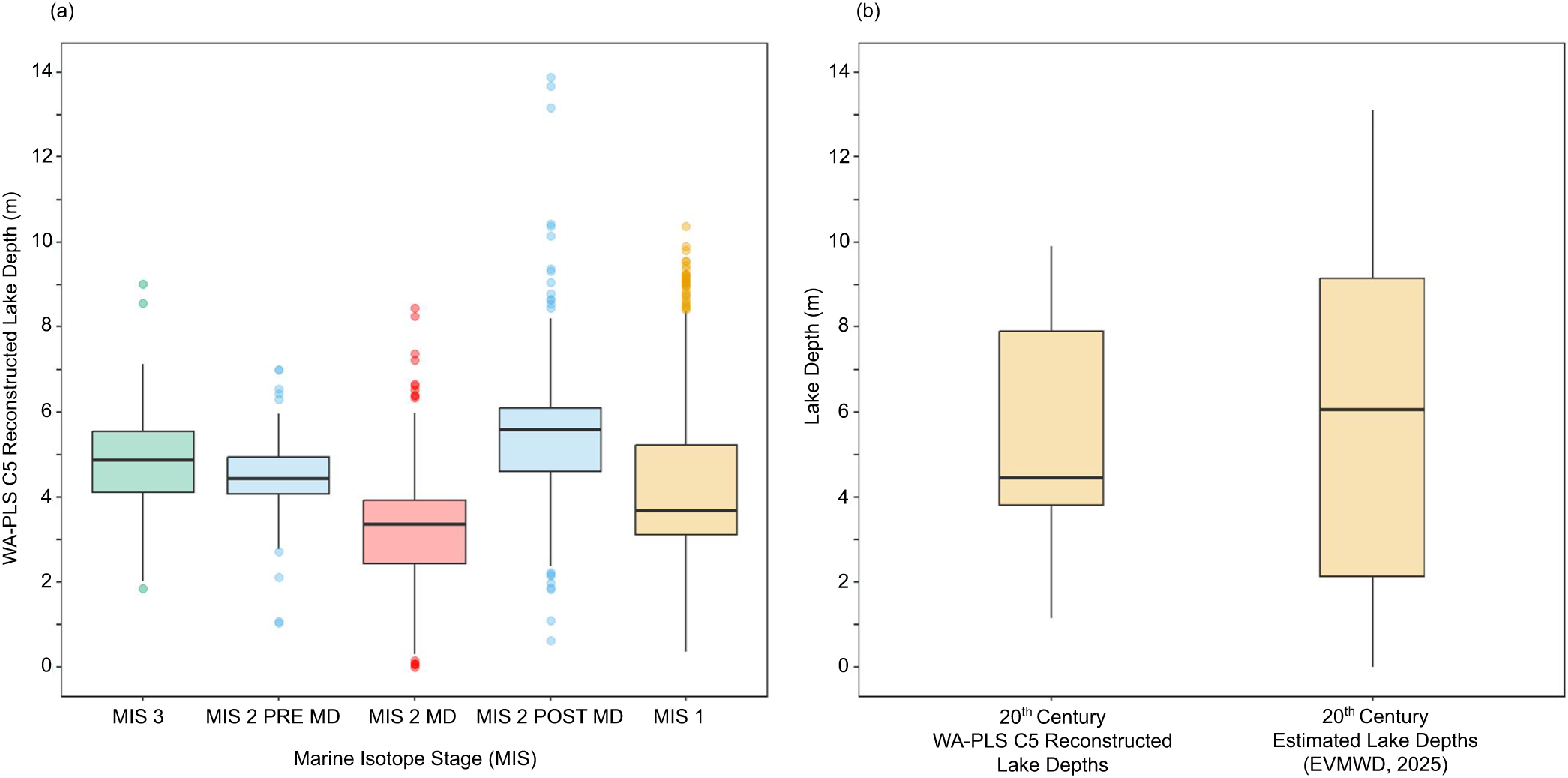
In general, lake depths are variable throughout the record, but have low values during MIS 1 relative to MIS 3 and most of MIS 2 (Figs. 8 and 9, Table 4). A sharp and extended decline in lake depth is observed near the start of MIS 2 (28,000 to 25,000 cal yr BP, MIS 2 mega-drought) (Heusser et al., Reference Heusser, Kirby and Nichols2015; Kirby et al., Reference Kirby, Heusser, Scholz, Ramezan, Anderson, Markle and Rhodes2018). The highest median in lake depths is recorded for the last glacial maximum and Heinrich Stadial 1 periods of MIS 2 (∼23,000-14,700 cal yr BP) following the MIS 2 mega-drought (Fig. 9). Notably, the Younger Dryas stadial (12,900–11,700 cal yr BP) exhibits an increase in lake depths followed by lower lake depths (Fig. 9). The lowest median lake depths occur during the MIS 2 mega-drought and in portions of MIS 1. Lake depths during MIS 3 and early MIS 2 are somewhat similar in terms of median and minimum values. Variability as measured by quartile spread around the median is highest in MIS 1 (Fig. 9). Changepoint analysis based on the 100 year binned reconstructed lake depths detected changes in long-term mean and variance, including near the bounds of the MIS 2 mega-drought (Fig. 8).
(a) Box plot of total variation in weighted averaging-partial least squares (WA-PLS) C5 reconstructed lake depths for Marine Isotope Stages. MIS 3 (32,000–29,000 cal yr BP), early MIS 2 before the MIS 2 mega-drought (MIS 2 PRE MD; 29,000–28,000 cal yr BP), MIS 2 mega-drought (MIS 2 MD; 28,000–25,000 cal yr BP), MIS 2 post-mega-drought (MIS 2 POST MD; 25,000–11,700 cal yr BP), and MIS 1 (<11,700 cal yr BP). (b) Box plots comparing twentieth-century reconstructed lake depths and twentieth-century estimated lake depths (EVMWD, 2025). The boxes represent the upper and lower 25% quartiles, with the thick horizontal lines indicating the medians. Whiskers extend to data within 1.5× the interquartile range. The colored points represent outliers.

Discussion
While elemental geochemistry in lacustrine environments is influenced by many complex factors, including detrital inputs shaped by local geology and hydrodynamic sorting, sedimentary processes in the water column and at the sediment–water interface, organic content and composition, and sediment grain size (Kong et al., Reference Kong, Tudryn, Gibert-Brunet, Tucholka, Motavalli-Anbaran, Lankarani, Ahmady-Birgani, Miska, Karimi and Dufaure2023; Bertrand et al., Reference Bertrand, Tjallingii, Kylander, Wilhelm, Roberts, Arnaud, Brown and Bindler2024), our study indicates that despite this complexity, elemental compositions in Lake Elsinore are significantly (P < 0.05, P < 0.01, and P < 0.001) statistically correlated with modern intra-lake water depths. The sediment distribution and elemental variation from shallow to deep zones at Lake Elsinore reflect a gradient of depositional environments, from sandy organic-poor shallows to clayey organic-rich deeps. The relationship between sediment chemistry and lake depth allows for a statistically based reconstruction of paleolake depth over the past 32,000 years that is consistent with other studies of the lake and region and known global forcing factors.
Elemental geochemistry distribution and relationship to lake depth and sedimentological variables
Sediment samples from shallow lake depth zones at Lake Elsinore reflect a high-energy depositional environment near the shoreline, characterized by sand-rich sediments and low organic content (Figs. 4 and 5). The generally high correlations among Ti, Mn, Fe, Sr, Rb, and Y suggest these elements are likely controlled by clastic inputs into the lake (Lu et al., Reference Lu, Fritz, Stone, Krause, Whitlock, Brown and Benes2017; Fig. 3). Elements such as Mn and Fe are most concentrated in this zone, closely following trends in grain size with strongest positive correlations to percent fine sand (Supplementary Fig. S2, r = 0.84, P < 0.001). Mn and Fe are prone to redox cycling and can exhibit complex behaviors in lakes (Hamilton-Taylor et al., Reference Hamilton-Taylor, Smith, Davison and Sugiyama2005). However, variations often reflect changes in grain size and/or sediment provenance in lakes (Bertrand et al., Reference Bertrand, Tjallingii, Kylander, Wilhelm, Roberts, Arnaud, Brown and Bindler2024). Mn and Fe oxides may be bound to trace elements such as Zn and Cu (El Bilali et al., Reference El Bilali, Rasmussen, Hall and Fortin2002) or absorb rare earth metals, such as Y, as part of terrigenous particles (Strakhovenko et al., Reference Strakhovenko, Belkina, Subetto, Rybalko, Efremenko, Kulik, Potakhin, Zobkov, Ovdina and Ludikova2023), concentrating them in the sediment. The elevated values of Ti and Zr are likely linked to their enrichment in coarse silt and fine sand fractions of sediments (Liu et al., Reference Liu, Bertrand and Weltje2019; Bertrand et al., Reference Bertrand, Tjallingii, Kylander, Wilhelm, Roberts, Arnaud, Brown and Bindler2024). Similarly, Rb and Sr in lake sediments can be sourced from physical erosion (Zeng et al., Reference Zeng, Chen, Xiao and Qi2013), and their strong presence in the coarse shallow-water sediments may be derived from the surrounding igneous and metamorphic rocks in the catchment area (Engel, Reference Engel1959). The relatively high levels of Ca and S in the shallow and mid-depth sediments likely reflect some combination of physical and biological controls on sedimentation. While the exact controls are not clear, some possible explanations for their high concentrations in these zones may include being introduced from erosion of surrounding rocks and soils, as Ca is likely associated with the igneous or metamorphic contributors in the coarse nearshore sediment and S is a common element in igneous rocks, and/or photosynthetic uptake of CO2 by phytoplankton, which can also facilitate CaCO3 precipitation within the epilimnion (Engel, Reference Engel1959; Anderson, Reference Anderson2001; Li et al., Reference Li, Xie, Zhang, Wang, Yang and Sun2016; Zhao et al., Reference Zhao, Zhang, Wang, Li, Ma, Chen, Deng and Annalisa2019).
The sediment samples from mid-depth zones reflect an intermediate depositional environment, bridging the highly energetic shallow zone and the more quiescent deeper basin (Figs. 4 and 5). This transition with increasing lake depths is marked by finer grain sizes, increased organic matter content, and a general decrease in Zn, Ti, Mn, Fe, Sr, Rb, Y, Zr, and Cu. Decreases in elements like Ti and Zr may be linked to the decrease of coarser grain sediments in the deeper, lower-energy lake zones, associated with finer grain sizes. The Ca/Fe ratio increases with depth in this transitional zone, suggesting that Ca is more abundant relative to Fe, possibly due to postsedimentary iron reduction (Pleskot et al., Reference Pleskot, Tjallingii, Makohonienko, Nowaczyk and Szczuciński2018).
Deep lake zones and associated sediment samples at Lake Elsinore are low-energy environments that favor clayey silts and accumulation of organic matter and total carbonate (Figs. 4 and 5). Increases in Th in the profundal zone of the lake may reflect its concentration in deeper, low-energy environments, as Th is associated with fine-grained sediments (Sakaguchi et al., Reference Sakaguchi, Yamamoto, Sasaki and Kashiwaya2006), and it is absorbed onto organic materials (Sheppard, Reference Sheppard1980). Fe, Ca, and Ti composition in sediment samples from the profundal sediments were generally lower than in samples from the littoral areas, which may be a result of decreased transport of coarse-grained terrigenous mineral material from the shore and anoxic processes leading to lower elemental values in sediments from the deeper lake sediments (Ikem and Adisa, Reference Ikem and Adisa2011). Lower elemental concentrations in the deeps may also result from dilution caused by the high concentrations of organic matter (Sabatier et al., Reference Sabatier, Moernaut, Bertrand, Van Daele, Kremer, Chaumillon and Arnaud2022).
Considerations regarding XRF-based lake depth transfer functions and paleolake depth reconstructions
XRF core scanning has emerged as a powerful tool for quickly, and nondestructively assessing high-resolution elemental geochemistry (Davies et al., Reference Davies, Lamb, Roberts, Croudace and Rothwell2015; Croudace et al., Reference Croudace, Löwemark, Tjallingii and Zolitschka2019; Bertrand et al., Reference Bertrand, Tjallingii, Kylander, Wilhelm, Roberts, Arnaud, Brown and Bindler2024), although several factors should be considered when interpreting these data and applying them to sediment records for paleohydrologic reconstructions. Certain elements may exhibit poor detection limits when using XRF core scanners, especially elements with low atomic numbers that produce low-energy radiation (Tjallingii et al., Reference Tjallingii, Röhl, Kölling and Bickert2007). Additionally, lake sediment elemental geochemistry from raw samples and cores can be affected by a range of complex factors, including variability in moisture content, grain size, provenance, and productivity (Tjallingii et al., Reference Tjallingii, Röhl, Kölling and Bickert2007; Löwemark et al., Reference Löwemark, Chen, Yang, Kylander, Yu, Hsu, Lee, Song and Jarvis2011; Bertrand et al., Reference Bertrand, Tjallingii, Kylander, Wilhelm, Roberts, Arnaud, Brown and Bindler2024). Furthermore, the mechanisms driving modern elemental composition in the lake sediments may change over time, particularly across glacial–interglacial cycles (Davies et al., Reference Davies, Lamb, Roberts, Croudace and Rothwell2015), and associated elements may couple and decouple over the history of the lake (Kylander et al., Reference Kylander, Ampel, Wohlfarth and Veres2011). Modern lake processes and elemental composition may not fully reflect past natural variability due to anthropogenic influence and modification. Therefore, due caution is encouraged when quantifying changes in lake depths based on modern elemental composition over millennia, and results are best considered semiquantitative. Despite these complications, the application of XRF to unprocessed marine, lake, and peat sediment cores has been widespread and has yielded important paleoenvironmental insights (Davies et al., Reference Davies, Lamb, Roberts, Croudace and Rothwell2015; Croudace et al., Reference Croudace, Löwemark, Tjallingii and Zolitschka2019; Kern et al., Reference Kern, Koutsodendris, Mächtle, Christanis, Schukraft, Scholz, Kotthoff and Pross2019). While findings from Lake Elsinore serve as a case study that indicates the promise of XRF approaches and the use of intra-lake calibration sets where there is a paucity of lake basins, each paleohydrologic study site must be investigated independently to assess its applicability for elemental-based lake depth reconstructions.
Evaluation of reconstructed lake depths and twentieth-century estimated lake depths based on historical records
The XRF-based lake depth transfer function performs well, but when it is applied to down-core assemblages, some reconstructed lake depths fall outside of the lake depth range in the calibration dataset (e.g., <1.4 m or >7.3 m) and should be used with caution. That being said, WA-PLS C5 reconstructed lake depths for the twentieth century fall within the range of observation, with a slight underestimation (EVMWD, 2025; Fig. 9). WA-PLS models tend to overestimate low values and underestimate high values (Birks, Reference Birks, Birks, Battarbee, Mackay and Oldfield2005). The range of lake depths estimated throughout the 32,000 year record fall within the range of variability observed over the twentieth-century historical period (Fig. 9).
Despite this similarity between the range of lake depth variability in both the reconstructed and twentieth-century historical periods, it is important to note the potential role of a lake’s ontogeny as a contributor to its long-term sediment record. In general, a basin’s accommodation space decreases over time in response to sediment infilling, thus modifying the basin’s geometry and influencing the long-term sedimentary signal. Even in tectonic pull-apart basins such as Lake Elsinore, sediment infilling occurs, assuming sedimentation rates exceed the basin’s rate of subsidence (Hull and Nicholson, Reference Hull and Nicholson1992; Kirby et al., Reference Kirby, Patterson, Ivanovici, Sandquist and Glover2021). However, the extent that these changes imprint on the long-term sediment signal is often specific to any given basin. For Lake Elsinore, we combine both sediment and seismic reflection data spanning 32,000 years (and longer if you consider pre-core depth seismic imaging) to assess the influence of changing accommodation space on the sediment record (Kirby et al., Reference Kirby, Heusser, Scholz, Ramezan, Anderson, Markle and Rhodes2018). Together, these data reveal no evidence for long-term lake depth shoaling (e.g., littoral zone progradation via basin contraction or shallowing) or a significant reduction in basin accommodation space (e.g., constricting stratal geometries) over the period of study (Kirby et al., Reference Kirby, Heusser, Scholz, Ramezan, Anderson, Markle and Rhodes2018). Both the former and latter might be expected in a basin where long-term sedimentation results in a volumetric loss that decreases the lake’s capacity to hold water or sediment and it ceases to act as a basin. The Elsinore sediment and seismic reflection data do not reflect the long-term signals associated with a loss in accommodation space. Rather the predominant sediment signals preserved in Lake Elsinore over the period of study are the large-amplitude changes in base level caused by the region’s characteristic “feast or famine” winter hydroclimate (Kirby et al., Reference Kirby, Poulsen, Lund, Patterson, Reidy and Hammond2004, Reference Kirby, Lund, Patterson, Anderson, Bird, Ivanovici, Monarrez and Nielsen2010, Reference Kirby, Feakins, Bonuso, Fantozzi and Hiner2013, Reference Kirby, Heusser, Scholz, Ramezan, Anderson, Markle and Rhodes2018, Reference Kirby, Patterson, Lachniet, Noblet, Anderson, Nichols and Avila2019). At shorter timescales (e.g., annual to multi-decadal), these changes influence sediment runoff, while at longer timescales (e.g., centennial to millennial), periods of sustained lake-level transgressions and regressions influence the distribution of fine versus coarse sediment associated with profundal versus littoral zone expansion or contraction. We conclude therefore that the lake’s ontogeny is not masking or modulating the changes in lake depth determined by our models presented in this paper. Of note, we limit our lake depth interpretations to the multi-decadal timescale, given the gross average sedimentation rate for the Lake Elsinore cores is 10.8 yrs/cm.
Lake Elsinore paleolake depth reconstruction and climatic drivers
The new Lake Elsinore paleolake depth reconstruction reinforces modern observations and prior paleo-research that illustrates the site’s hydroclimatic sensitivity and responsiveness to large-scale climatic drivers, including orbitally induced variations in seasonal latitudinal insolation (Fig. 9, Table 4). MIS 3 is typified by lake depths that are somewhat intermediate between the high last glacial maximum (MIS 2) and low Holocene depths (MIS 1). During early MIS 2, lake depths shallow rapidly and remain low (Fig. 9, Table 4). This reconstructed decrease in lake depths in early MIS 2 corresponds to a nearly 2000 year glacial mega-drought inferred from previous analysis of the Lake Elsinore sediments using pollen (Heusser et al., Reference Heusser, Kirby and Nichols2015), grain size (Kirby et al., Reference Kirby, Heusser, Scholz, Ramezan, Anderson, Markle and Rhodes2018), and organic geochemistry (Feakins et al., Reference Feakins, Wu, Ponton and Tierney2019). Kirby et al. (Reference Kirby, Heusser, Scholz, Ramezan, Anderson, Markle and Rhodes2018) used modern lake depth and lake bottom surface grainsize relationships to estimate an average lake depth of 3.7 m with a 95% range of 3.2–4.5 m during the Elsinore MIS 2 mega-drought; these independent lake depth estimates are similar to the median and average lake depth estimates based on this study (median: 3.35 m; mean: 3.25 ± 1.52 m) using modern lake depths and XRF-based elemental geochemistry relationships. Although the MIS 2 mega-drought is a singular feature within the lake’s history, these two independent methods, which generate similar lake depth results for this period, provide confidence in the XRF methodology presented here. Regionally, a contemporaneous MIS 2 mega-drought is observed in the sedimentary pollen record from Baldwin Lake in the San Bernardino Mountains, approximately 75 km to the northeast and at higher elevation (2060 m) than Elsinore (Glover et al., Reference Glover, Chaney, Kirby, Patterson and MacDonald2020). Further south in California, a noble gas isotope–derived groundwater table depth reconstruction reveals a substantial drop in water tables possibly correlative (within groundwater dating errors) to the lake-observed MIS 2 mega-drought (Seltzer et al., Reference Seltzer, Ng, Danskin, Kulongoski, Gannon, Stute and Severinghaus2019).
During the MIS 2 post-mega-drought period encapsulating the last glacial maximum (∼23,000–19,000 cal yr BP) and Heinrich Stadial 1 (∼18,000–14,700 cal yr BP), lake depths were variable but consistently deeper than in any other period (MIS 1 or 3) in the 32,000 year record, likely due to wetter conditions combined with colder temperatures and less evaporation (Lora and Ibarra, Reference Lora and Ibarra2019; Palacios et al., Reference Palacios, Stokes, Phillips, Clague, Alcalá-Reygosa, Andrés and Angel2020; Tulenko et al., Reference Tulenko, Lofverstrom and Briner2020; Fig. 9, Table 4). MIS 1 (i.e., Holocene) lake depths are the lowest in the record, excluding the MIS 2 mega-drought, but exhibit larger-amplitude variability, suggesting shallow to intermediate lake depths with occasional high stands, accordant with historical Lake Elsinore lake depth variability (Kirby et al., Reference Kirby, Lund, Anderson and Bird2007, Reference Kirby, Patterson, Lachniet, Noblet, Anderson, Nichols and Avila2019). Overall, the results are consistent with a wetter, cooler, and/or less evaporative late last glacial (MIS 3–2), excepting the anomalous MIS 2 mega-drought, than the Holocene in the interior Southwest and coastal Southwest United States (Wagner et al., Reference Wagner, Cole, Beck, Patchett, Henderson and Barnett2010; Kirby et al., Reference Kirby, Feakins, Bonuso, Fantozzi and Hiner2013; Oster et al., Reference Oster, Ibarra, Winnick and Maher2015; Lora and Ibarra, Reference Lora and Ibarra2019). Perhaps most insightful, our inferred lake depth record reveals a dynamic, highly variable lake over the past 32,000 years, fitting with historical observations and California’s volatile or “whiplash” winter–dominated hydroclimate (Swain et al., Reference Swain, Langenbrunner, Neelin and Hall2018).
We also compare our lake depth reconstruction to the Kirby et al. (Reference Kirby, Heusser, Scholz, Ramezan, Anderson, Markle and Rhodes2018) sand-runoff data. At Lake Elsinore, higher percent sand typically reflects greater precipitation-related runoff (i.e., storm intensity and/or duration); whereas lower percent sand reflects diminished runoff (Kirby et al., Reference Kirby, Lund, Patterson, Anderson, Bird, Ivanovici, Monarrez and Nielsen2010, Reference Kirby, Heusser, Scholz, Ramezan, Anderson, Markle and Rhodes2018; Fig. 8). Based on this model, higher percent sand is interpreted to reflect wetter winters and vice versa for lower percent sand. However, the sand-runoff interpretation does not explain the anomalously high sand content unit observed during the MIS 2 mega-drought (Fig. 8). As detailed by Kirby et al. (Reference Kirby, Heusser, Scholz, Ramezan, Anderson, Markle and Rhodes2018), this high sand unit reflects a prolonged period of low lake levels where the lake’s size and mud depth boundary contracted, leading to the basinward progradation of the coarse-sediment littoral zone. In general, the Lake Elsinore percent sand data as a runoff indicator (i.e., winter wetness proxy) support the lake depth reconstruction and show a range of hydroclimatic variability over the 32,000 year record, with generally more runoff during MIS 3 and 2, excluding the mega-drought, and more variable, but overall lower runoff during MIS 1/Holocene.
Lake Elsinore’s hydroclimate over the past 32,000 years likely reflects a combination of complex external climatic drivers, including changes in insolation, continental ice sheet extent/configuration, and coupled ocean–atmosphere dynamics (Kirby et al., Reference Kirby, Lund, Anderson and Bird2007, Reference Kirby, Feakins, Bonuso, Fantozzi and Hiner2013; Fig. 8). Today, Lake Elsinore’s annual water levels respond rapidly to the balance between winter precipitation and summer-to-early fall evaporation, reflecting the precipitation-to-evaporation (P:E) ratio and its modulation of lake depth (Kirby et al., Reference Kirby, Lund, Patterson, Anderson, Bird, Ivanovici, Monarrez and Nielsen2010, Reference Kirby, Patterson, Lachniet, Noblet, Anderson, Nichols and Avila2019). At longer timescales, the lake similarly reacts to changes in the P:E ratio but in response to variations in lower-amplitude and sometimes far-field climatic drivers such as orbital changes in seasonal latitudinal insolation, hemispheric temperatures, and northern and tropical Pacific sea-surface temperature (SST) variability (Kirby et al., Reference Kirby, Lund and Poulsen2005, Reference Kirby, Lund, Anderson and Bird2007, Reference Kirby, Lund, Patterson, Anderson, Bird, Ivanovici, Monarrez and Nielsen2010, Reference Kirby, Feakins, Bonuso, Fantozzi and Hiner2013; Heusser et al., Reference Heusser, Kirby and Nichols2015; Feakins et al., Reference Feakins, Wu, Ponton and Tierney2019; Fig. 8). Changing North American ice sheet extent driven by orbital variations also influenced atmospheric circulation, with an expanded ice sheet strengthening latitudinal temperature gradients and shifting the circumpolar vortex south of its current position during the Late Pleistocene and into the early postglacial (Bartlein et al., Reference Bartlein, Anderson, Anderson, Edwards, Mock, Thompson, Webb, Webb and Whitlock1998; Oster et al., Reference Oster, Ibarra, Winnick and Maher2015; Löfverström and Lora, Reference Löfverström and Lora2017). These changes likely led to greater frequency of winter storms along the central and Southern California coast during MIS 2 (Kirby et al., Reference Kirby, Feakins, Bonuso, Fantozzi and Hiner2013; Oster et al., Reference Oster, Ibarra, Winnick and Maher2015; Morrill et al., Reference Morrill, Lowry and Hoell2018). The large-scale reorganization of terrestrial heat balance, glacial ice cover, and the ocean–atmosphere system produced long-term climatic regimes in Southern California with cooler temperatures, less evaporation, and possibly increased winter precipitation during most of MIS 2, generating a robust pluvial regime (MIS 2 post-mega-drought at Lake Elsinore) during the late glacial (Mensing, Reference Mensing2001; Wells et al., Reference Wells, Brown, Enzel, Anderson and McFadden2003; Kirby et al., Reference Kirby, Feakins, Bonuso, Fantozzi and Hiner2013; Morrill et al., Reference Morrill, Lowry and Hoell2018; Lora and Ibarra, Reference Lora and Ibarra2019). These external drivers are reflected in the generally greater lake depths at Lake Elsinore for much of MIS 2 post-mega-drought (Figs. 8 and 9). The last deglaciation and transition from MIS 2 to MIS 1 was a period of abrupt and major climatic reorganizations with profound impacts on temperature, hydrology, and ecology in the western United States and Lake Elsinore region (Kirby et al., Reference Kirby, Feakins, Bonuso, Fantozzi and Hiner2013, Reference Kirby, Heusser, Scholz, Ramezan, Anderson, Markle and Rhodes2018; Heusser et al., Reference Heusser, Kirby and Nichols2015; Lora et al., Reference Lora, Mitchell and Tripati2016; Hudson et al., Reference Hudson, Hatchett, Quade, Boyle, Bassett, Ali and De Los Santos2019; Fu, Reference Fu2023; O’Keefe et al., Reference O’Keefe, Dunn, Weitzel, Waters, Martinez, Binder and Southon2023). In contrast to MIS 2, MIS 1, characterized by a minimum of glacial ice cover in the Northern Hemisphere, along with a decrease in winter storm frequency due to the modulation of the winter-season Pacific storm track by changing ice sheet extent and broadscale modulation of Pacific SSTs, likely promoted warmer and drier winter conditions in Southern California (Enzel et al., Reference Enzel, Brown, Anderson, McFadden and Wells1992; Mensing, Reference Mensing2001; Lora et al., Reference Lora, Mitchell and Tripati2016; Hudson et al., Reference Hudson, Hatchett, Quade, Boyle, Bassett, Ali and De Los Santos2019; Kirby et al., Reference Kirby, Patterson, Lachniet, Noblet, Anderson, Nichols and Avila2019; Lora and Iberra, Reference Lora and Ibarra2019; Fu, Reference Fu2023). MIS 1 coincides with shallower median, but highly dynamic, lake depths by comparison to MIS 3 and most of MIS 2 at Lake Elsinore (Fig. 9).
Tropical and northern Pacific Ocean SSTs, in particular, play an important role in the winter hydroclimate of Southern California and the Lake Elsinore region. Warm SSTs in the eastern tropical and northern extra-tropical Pacific relative to the western Pacific are generally associated with increased precipitation in Southern California varying from interannual to millennial timescales (Wise, Reference Wise2010; Kirby et al., Reference Kirby, Knell, Anderson, Lachniet, Palermo, Eeg and Lucero2015; Hoell et al., Reference Hoell, Hoerling, Eischeid, Wolter, Dole, Perlwitz, Xu and Cheng2016; Cheng et al., Reference Cheng, Novak and Schneider2021). Comparison of the Lake Elsinore record to evidence of changes in the strength of the west to east gradient in the tropical Pacific over the past 30,000 years (Koutavas and Joanides, Reference Koutavas and Joanides2012) indicates a relationship between weakening of the gradient (relative warming eastern Pacific compared with western Pacific = El Niño–like conditions) and greater lake depth at Lake Elsinore. In contrast, a strengthening of the gradient (relative cooling of the eastern Pacific relative to western Pacific = La Niña–like conditions) leads to decreased lake depth at Lake Elsinore (Fig. 8). Winter rainfall anomalies (e.g., generally higher precipitation) in Southern California are positively correlated with El Niño conditions, although this relationship accounts for at most 33% of the observed variance and is dependent on the intensity or state of the specific El Niño event (Cash and Burls, Reference Cash and Burls2019; Byrne et al., Reference Byrne, Merrifield, Carter, Cayan, Flick, Gershunov and Giddings2023). Dry winters are more likely during La Niña events (Byrne et al., Reference Byrne, Merrifield, Carter, Cayan, Flick, Gershunov and Giddings2023). Moreover, high ratios of dextral to sinistral Neoglobquadrina pachyderma from the Santa Barbara Basin indicate warm SSTs (Hendy, Reference Hendy2010), which generally align with decreasing lake depths at Lake Elsinore (e.g., MIS 1), whereas low ratios correspond to cooler SSTs and increasing lake depths at Lake Elsinore (e.g., MIS 2 post-mega-drought) (Fig. 8). This may reflect a relationship between regional temperatures and lake depth, indicative of evaporative influences on water balance. These patterns are particularly clear in the contrast between MIS 2 last glacial maximum conditions and conditions during MIS 1. Although dating is more uncertain at the time of the early MIS 2 mega-drought, it appears that at least the onset of the MIS 2 mega-drought corresponds to a marked increase in the strength of the tropical Pacific W-E SST gradient (i.e., more La Niña–like conditions) and warmer temperatures in the Santa Barbara Basin. Similarly, the Bølling-Allerød Interstadial (14,700–12,900 cal yr BP) appears to correspond to an increase in the strength of the tropical Pacific W-E SST gradient, the rapid warming of SSTs in the Santa Barbara Basin, and a decrease in lake depths at Lake Elsinore (Fig. 8). The Bølling-Allerød is terminated by an abrupt increase in lake depth with colder Santa Barbara Basin SSTs at the onset of the Younger Dryas stadial (12,900–11,700 cal yr BP) followed by an abrupt decrease in lake depth and warmer Santa Barbara Basin SSTs midway through the Younger Dryas (Fig. 8). Evidence for a similar multistate hydroclimatic pattern (wet/dry) during the Younger Dryas is observed elsewhere in California, such as Lake Bennett and Starkweather Lake in the Sierra Nevada Mountains (MacDonald et al., Reference MacDonald, Moser, Bloom, Porinchu, Potito, Wolfe, Edwards, Petel, Orme and Orme2008), Barley Lake in northwest California (Leidelmeijer et al., Reference Leidelmeijer, Kirby, MacDonald, Carlin, Avila, Han, Nauman, Loyd, Nichols and Ramezan2021), Owens Lake (Benson et al., Reference Benson, Burdett, Lund, Kashgarian and Mensing1997; Mensing, Reference Mensing2001; Bacon et al., Reference Bacon, Burke, Pezzopane and Jayko2006; Orme and Orme, Reference Orme and Orme2008), and various Mojave Desert wetland deposits (Pigati et al., Reference Pigati, Springer and Honke2019; Pigati and Springer, Reference Pigati and Springer2022). Subsequent to the Younger Dryas, MIS 1/Holocene is typified by warmer global temperatures, generally strong tropical Pacific W-E SST gradient, warm SSTs in the Santa Barbara Basin, and low but variable depths at Lake Elsinore.
Conclusions
Variations in the elemental geochemistry composition in Lake Elsinore modern intra-lake surface sediment samples are significantly correlated with differences in lake depth. Three distinct lake depth zones were identified based on modern elemental geochemistry assemblages and lake depth relationships: shallow (1.4–3.58 m), mid-depth (3.58–5.17 m), and deep (5.17–7.3 m). The statistically robust relationship between modern surface sediment elemental geochemistry and lake depth was used to develop a 32,000 year reconstruction of lake depths using down-core XRF measurements at Lake Elsinore. The substantial variations in reconstructed lake depths spanning late MIS 3 through to 1993 CE are consistent with the large-scale climatic changes related to the MISs and highlight the climatic sensitivity of the site and the potential of using nondestructive and rapid XRF core-scanning data with intra-lake training sets for paleohydrologic reconstructions. While the Elsinore record serves as a case study that indicates the promise of XRF-based intra-lake depth calibration sets and down-core lake depth transfer function reconstructions, each lake and elemental geochemical assemblage is unique and XRF-based analyses should be developed on a site-specific basis.
The 32,000 year lake depth reconstruction conforms with historical observations that small changes in winter precipitation and/or summer evaporation generate highly dynamic lake depth responses and indicates the high degree of sensitivity of Lake Elsinore to external climatic drivers and internal, coupled ocean–atmosphere interactions, including orbital changes in seasonal latitudinal insolation, hemispheric temperatures, and northern and tropical Pacific SSTs. Notably, the lake depth record indicates a prolonged early MIS 2 mega-drought (28,000–25,000 cal yr BP), generally deep lake depths during the last glacial maximum (∼23,000–19,000 cal yr BP) and Heinrich Stadial 1 (∼18,000–14,700 cal yr BP), a wet–dry pattern response to the Younger Dryas (12,900–11,700 cal yr BP), and a more variable but generally drier MIS 1/Holocene (<11,700 cal yr BP). The hydroclimatic sensitivity of Lake Elsinore over the past 32,000 years gives important insights into past climate dynamics. The Lake Elsinore XRF-based lake depth reconstruction may provide analogs to future lake responses to anthropogenic climate changes.
Supplementary material
The supplementary material for this article can be found at https://doi.org/10.1017/qua.2026.10074.
Acknowledgments
This work was financially supported by the UCLA Geography of California and the American West Endowment, the National Science Foundation (nos. 031511, 0731843, 1203549), and the American Chemical Society Petroleum Research Fund (no. 4187-B8). We thank Jessie George, Benjamin Nauman, and Nicholas Burdy for their assistance during fieldwork. We thank the editors (Nicholas Lancaster and Lesleigh Anderson) and two anonymous reviewers for their helpful feedback and edits.


 Open access