2.1. Ice draft and velocity measurements from under-ice moorings

Two moorings (B1 and B2) were deployed near Barrow, Alaska, USA, as part of SIZONet (Fig. 1). Mooring B1 was deployed at 71.32698°N, 156.87663°W on 5 August 2009 and retrieved on 29 July 2010. Mooring B2 was deployed at 71.23471° N, 157.65271° W on 7 August 2009 and retrieved on 29 July 2010. These moorings each comprised an ASL Environmental Science Ice Profiler IPS and a Teledyne RDI Workhorse Sentinel ADCP as well as a Seabird SBE-37 conductivity–temperature (C-T) recorder and a Seabird SBE-39 temperature–pressure (T-P) recorder (Fig. 2). The IPSs are used to measure the draft of the sea ice passing overhead while the ADCPs measure current velocity profile of the overlying water column and, of particular relevance here, the velocity of the ice through bottom tracking.

Fig. 1.

AEM flight path over mooring B2 on 12 April 2010 near Barrow, Alaska. Also shown are the locations of mooring B1, an ice mass-balance site (MBS) and the approximate range of a coastal sea-ice radar system installed on a building in Barrow. The background is a Wide Swath Envisat ASAR image acquired 1 hour after the AEM flight passed over mooring B2.

Fig. 2.

Configuration of SIZONet moorings deployed near Barrow in 2009/10. Distances indicate approximate rope lengths between mooring components.

The calculation of ice draft from raw IPS data is an involved process, described in detail by Reference Melling, Johnston and RiedelMelling and others (1995). In brief, the distance from the sonar to the ice or open-water surface is determined from the travel time of echoes, with adjustments made for instrument tilt. Corrections for sound-speed variations over time are made by identifying open water above the sonar and reconciling the measured echo travel time with the depth determined from an onboard pressure sensor. Through this approach, the draft of the level ice can be measured to an estimated accuracy and precision of ±0.05 m (Reference Fukamachi, Mizuta, Ohshima, Toyota and KimuraFukamachi and others, 2006). Ice draft measurements are made at 1 s intervals.

A moored IPS generates a time series of ice draft at a fixed location as the sea ice drifts overhead. Since the drift velocity of the ice is not constant over time, these data cannot be used to derive distance-referenced probability distributions. It is therefore necessary to transform the time series into a pseudo-spatial series using ice velocity data. In our case we use ice velocities calculated from the ADCP bottom track data. The ice velocity is determined from the Doppler shifts of acoustic signals returned from the bottom of the ice. This is similar to the method used to determine the water velocity, but a separate longer-pulse signal is used to achieve accuracies of a few mms–1 (Gordon, 1996).

The bottom track data are recorded every 15 min and so must be interpolated to match the 1 s time series recorded by the IPS. Each interpolated velocity measurement thus represents an effective sampling distance for each ice draft measurement. We then use a cubic spline interpolation to create a regularly spaced pseudo-spatial series of ice draft with 1 m spacing, approximately matching the footprint of the sonar beam on the underside of the ice (Reference WilliamsWilliams and others, 2008). The measurement of ice draft can be related to ice thickness by invoking Archimedes’ principle, with the total weight of the ice and snow equal to the weight of the water displaced. If we assume that the ice at each measurement is in isostatic equilibrium, then this can be expressed as

where pi, p _s and p _w are the densities of ice, snow and water, respectively. Zi and Zs are the thicknesses of ice and snow, respectively, and D is the ice draft.

2.2. Airborne electromagnetic (AEM) ice thickness measurements

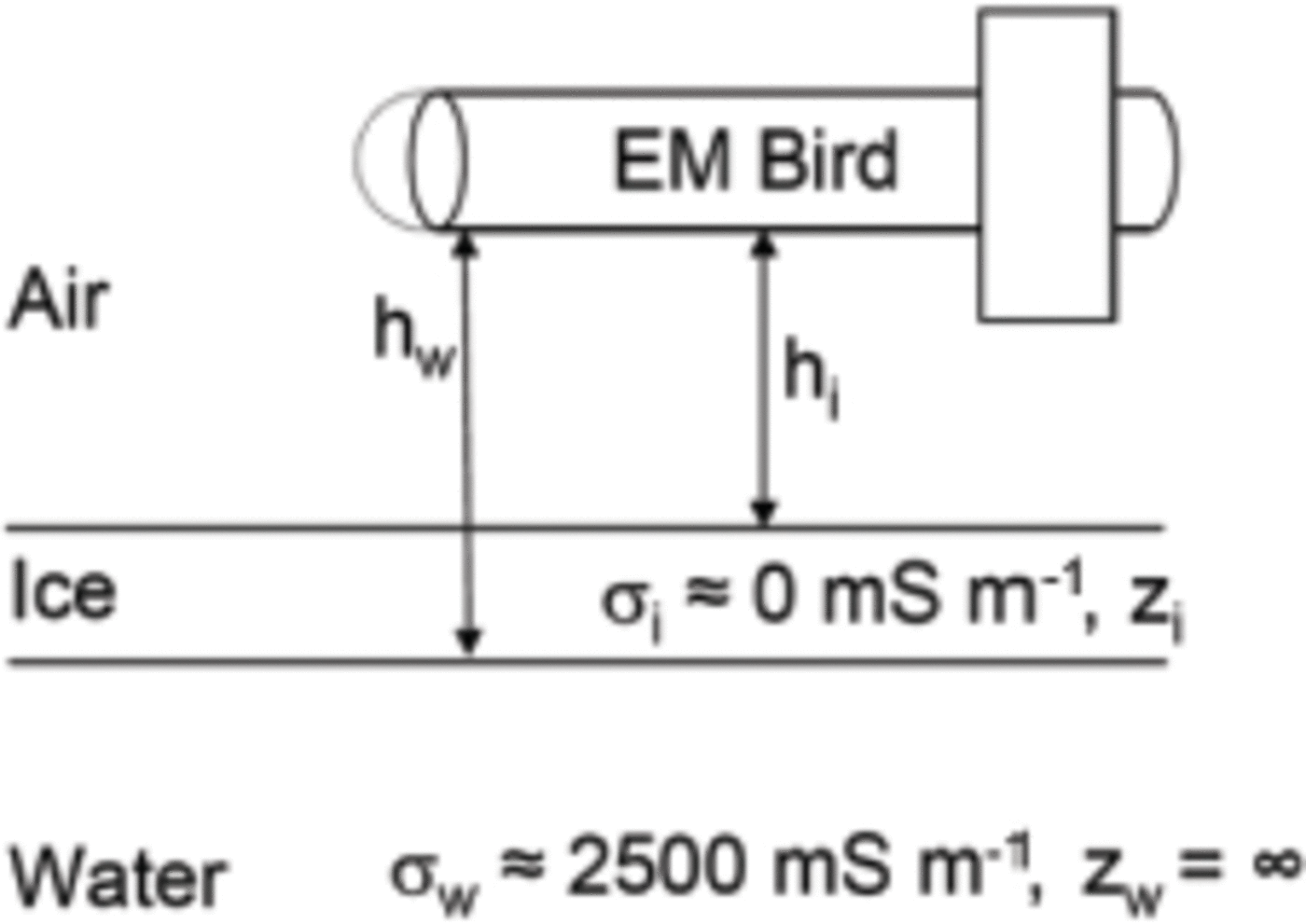
AEM sounding uses electromagnetic (EM) induction to determine the distance from the towed instrument, known as an EM-bird, to the water surface (Reference Haas, Lobach, Hendricks, Rabenstein and PfafflingHaas and others, 2009, Reference Haas, Hendricks, Eicken and Herber2010). The technique involves emitting a primary EM field (in this case at 4.09 kHz), which induces a secondary field in the conductive sea water. Using a one-dimensional model in which the sea-water and sea-ice conductivities are specified (Reference Pfaffling and HaasPfaffling and others, 2007), the distance to the underside of the ice can be determined from the relative strength of the in-phase component of the secondary field. At the same time, the distance to the upper surface of the ice (or snow if present) is measured using a laser altimeter mounted in the EM-bird. The combined thickness of snow and sea ice is determined by subtracting these two distances (Fig. 3). In comparison with field measurements, this technique is found to have an accuracy of better than 0.1 m over level ice (Reference Haas, Lobach, Hendricks, Rabenstein and PfafflingHaas and others, 2009).

Fig. 3.

From Reference Haas, Lobach, Hendricks, Rabenstein and PfafflingHaas and others (2009). Principle of AEM thickness sounding, using a bird with transmitter and receiver coils and a laser altimeter. Ice thickness Z _i is obtained from the difference between measurements of the bird’s height above the water and ice surface, h _w and h _i, respectively.

Fig. 4.

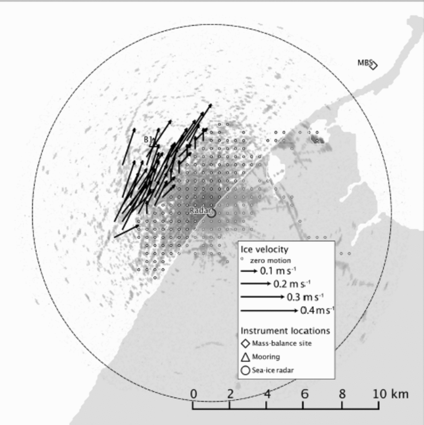
Coastal radar image acquired at 21:25 on 12 April 2010 (UTC), coincident with the Envisat ASAR image in Figure 1. Vectors show ice velocities determined from consecutive images.

In April 2010, two AEM flights were made over the sea ice near Barrow as part of SIZONet activities. On 12 April 2010, the flight path passed twice over mooring B2 (Fig. 1). A helicopter was used for these flights, allowing us to make controlled, tight turns over the mooring location. The EM-bird was flown at an altitude of ∼15 m, giving an effective sampling footprint of ∼70 m. Each AEM measurement is thus a mean value of ice and snow thickness over this area. The EM-bird will therefore tend to underestimate the maximum thickness of ice ridges, though it can be expected to give an accurate measure of the overall ice volume (Pfaffling and others, 2007).

2.3. Gridded ice velocities from coastal sea-ice radar data

The University of Alaska Fairbanks (UAF) has operated a coastal sea-ice radar discontinuously since the 1970s (Reference Shapiro and MetznerShapiro and Metzner, 1989; Reference Mahoney, Eicken and ShapiroMahoney and others, 2007; Reference Druckenmiller, Eicken and JohnsonDruckenmiller and others, 2009; Reference JonesJones, 2013; Reference Rohith, Jones, Eicken and KambhamettuRohith and others, 2013). Data from the current system are available in near real time from http://seaice.alaska.edu/gi/observatories/barrow_radar. Figure 4 shows an image from the radar on 12 April 2010 coinciding with the Envisat Advanced Synthetic Aperture Radar (ASAR) image shown in Figure 1. The coastal radar has a considerably lower grazing angle than space-based systems and is reliant on rough surfaces with higher local incidence angles to act as natural reflectors. The coastal radar is therefore mostly sensitive to ridges and floe edges, with little or no energy returned from areas of level ice in between. As a result, images from the coastal radar often contain ‘empty’ regions without features that can be tracked through commonly used techniques based upon cross-correlation of image pairs. To overcome these challenges, we use a combination of dense and sparse optical flow methods to generate gridded ice velocities (Reference Rohith, Jones, Eicken and KambhamettuRohith and others, 2013)

The radar data are recorded in range-azimuth space with 512 samples per range line and up to 4096 lines per rotation. The calculation of velocity in physical units requires accurate geolocation of the radar imagery. We determined the correct range resolution and orientation of the imagery using linear ground control features such as pipelines, roads and snow fences that were recognizable in both the radar imagery and high-resolution satellite data available through the Geographic Information Network of Alaska (GINA). At a nominal range setting of 6 nautical miles, we determined the range resolution to be 21.5 ± 0.5 m, which is the pixel size chosen for reprojection of the data to a Cartesian plane. The radar system records images every 120 rotations, which at a rotation speed of ∼0.5 Hz corresponds to ∼4 min between images although this interval is variable due to small changes in rotation speed of the radar antenna. Since the file creation times for each radar image are only preserved to an accuracy of 1 min, it is therefore difficult to precisely determine the time interval over which motion is observed. However, over the whole record for the 2009/10 season, we calculate an average interval between consecutive images of 231 ± 9 s . Together, these uncertainties in spatial scale and time interval amount to a 5% error in the radar-derived velocitiesFig. 4. Coastal radar image acquired at 21.25 on 12 April 2010 (UTC), coincident with the Envisat ASAR image in Figure 1 . Vectors show ice velocities determined from consecutive images.

The velocity vectors shown in Figure 4 are calculated on a 2 0 x 2 0 pixel (438 m x 438 m) grid and have been median-filtered in time to remove erroneous values (this procedure is discussed in more detail in Section 3). Gridpoints with zero velocity are shown by white dots and indicate the extent of landfast ice at the time of data acquisition. Gridpoints where no velocity measurement could be determined are blank. Velocity determination typically fails due to one of three causes: (1) a lack of reflectors; (2) excessive ice motion; or (3) rapid changes in reflector orientation or shape due to ice movement or deformation. For the purposes of comparing radar-derived ice velocities with the bottom track data recorded by the ADCP, we calculate the mean velocity recorded at the four gridpoints surrounding mooring B1.

Table 1.

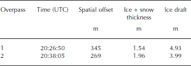
Time, closest distance and coincident measurements for AEM overpasses 1 and 2

3.1. Ice thickness over mooring B2

Figure 5 shows the path of the AEM flight on 12 April 2010 (in white) over mooring B2 together with a pseudo-track of ice motion (in gray) derived by integrating the bottom track velocity recorded by the ADCP forward and backwards in time from the time of the AEM overpass. The continuous white lines indicate portions of the flight made at measurement altitude within a 10km radius of the mooring (shown by the black dashed circle). The white dots indicate the calculated 6 hourly positions along the pseudo-track. The helicopter made two separate overpasses, which are indicated by the labeled arrows. Table 1 lists the time and distance of the closest point on each overpass together with the AEM-derived ice thickness and the IPS-measured ice draft at the times. The background is the Envisat ASAR image shown in Figure 1, which was acquired at 21.26.59 UTC (coordinated universal time) on 12 April, just 1 hour after the first overpass. The black cross indicates the location of ice that was at the mooring at the time of overpass 1, based on the pseudo-track data.

Fig. 5.

Map showing the AEM flight path over mooring B2. The gray line indicates a pseudo-track of ice drift calculated by integrating the bottom track velocity overtime. White dots indicate the 6 hourly pseudo-positions of the ice before and after the overpass. Only those at ±6 and 12 hours are labeled, to reduce clutter in the figure. The black cross indicates ice that was at the mooring at the time of overpass 1.

Table 1 shows significant differences between the coincident AEM and IPS measurements at the time of each overpass. In both cases the IPS-measured draft is greater than the AEM-measured combined snow and ice thickness. In some cases such differences can be accounted for by the larger sampling footprint of the EM-bird, if there happened to be a narrow ridge keel above the IPS at the time of the overpass, the thickness of which would be underestimated in the AEM data. However, examination of the IPS before and after each overpass indicates this is not the case. Instead, it is more likely the difference is due to the spatial offset between the actual measurement locations. This is supported by the SAR image in Figure 5, which shows high backscatter in the region of the mooring at the time of the overpass (marked by black cross), indicating rough, heterogeneous ice.

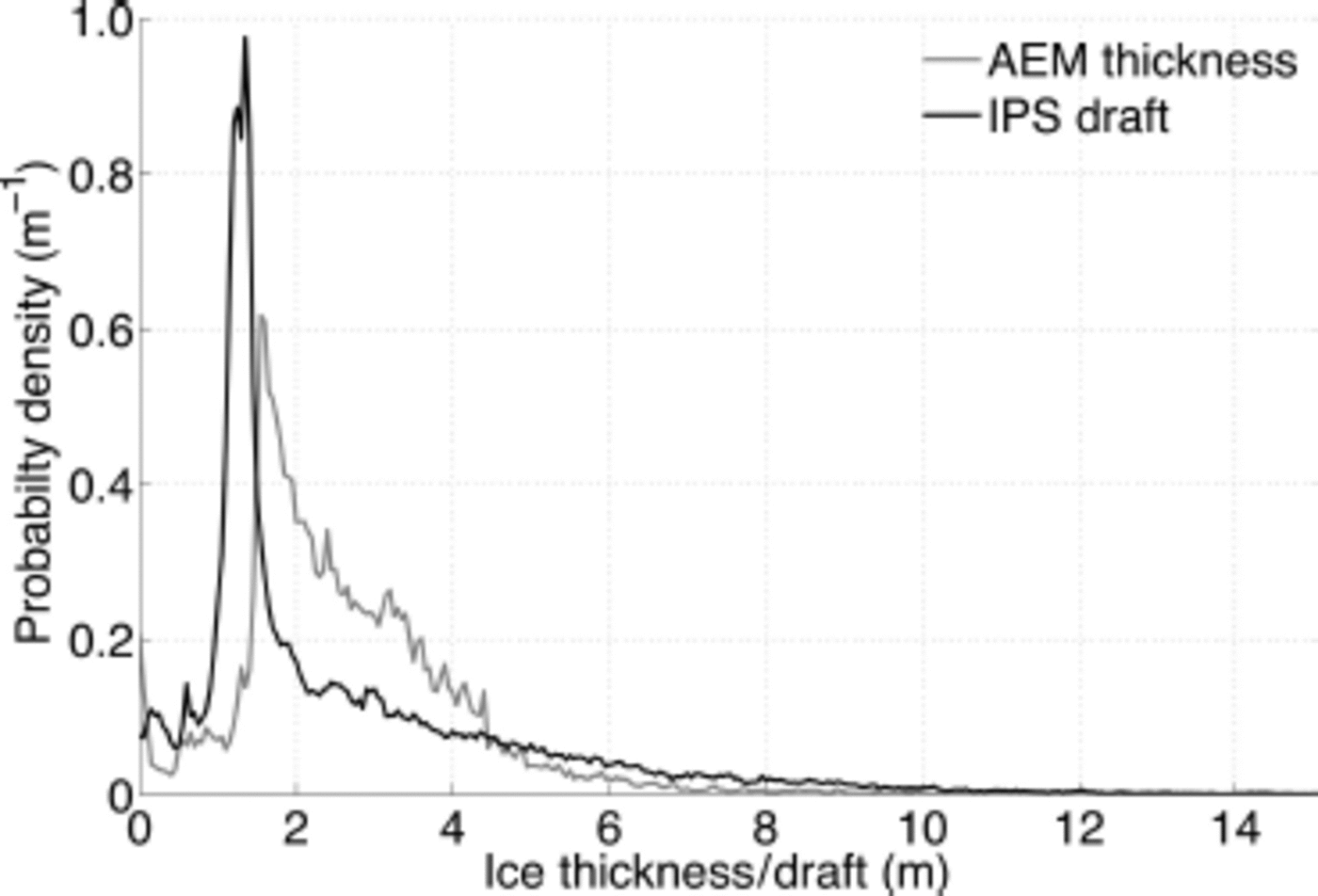
Neither of the overpasses was aligned with the drift of ice at the time, which means it is not feasible to attempt to co-locate the measurements more accurately. We therefore compare AEM and IPS measurements by calculating their probability distributions using all data that fall within 10 km of mooring B2 (indicated by the black dashed circle in Fig. 5). Figure 6 shows the distributions of AEM-derived ice and snow thickness and IPS-derived ice draft, binned into 0.05 m intervals. Both distributions have pronounced modes, which represent the thickness and draft of level undeformed ice. The AEM data indicate a modal combined thickness of ice and snow of 1.6±0.025 m while the IPS data show a modal ice draft of 1.35 ± 0.025 m. These values and their relationship with density and snow depth are discussed in more detail below.

Fig. 6.

Probability distribution of combined ice and snow thickness (AEM) and ice draft (IPS) derived from all measurements within 10km of mooring B2.

3.2. Ice velocities near Barrow during 2009/10 winter season

A comparison of radar-derived and ADCP bottom-tracked ice velocities was carried out for mooring B1 for the period 1 November 2009 to 30 June 2010 (Fig. 7). We binned the radar-derived values every 15 min to match the sampling interval of the ADCP. We have also excluded data from periods with a significant open-water fraction and when the instrument tilt exceeded 20°. The presence of open water can be inferred from increased magnitude and variability of the bottom track error recorded by the ADCP due to the presence of surface waves (Reference Belliveau and BugdenBelliveau and others, 1990). We applied a 2 hour running mean to the bottom track error values and discarded data from periods with error values greater than 0.1 m s–1.

Fig. 7.

Scatter plots comparing ADCP- and radar-derived ice velocities for winter 2009/10: (a) velocity magnitude; (b) alongshore velocity component; (c) offshore velocity component.

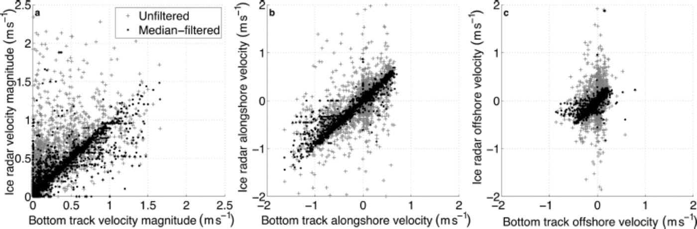
The radar-derived velocities show significant scatter and that the optical flow algorithm tends to overestimate ice speed as compared to bottom-tracked ice velocities. However, we see considerably better agreement when we apply a 2 hour running median filter to the radar-derived data, with tighter clustering around the line y=x and an improvement in the root-mean-square (rms) difference in velocity magnitudes from 0.24 m s^–1 to 0.12 ms^–1. The close agreement in both alongshore and offshore components indicates that both datasets are well aligned geographically.

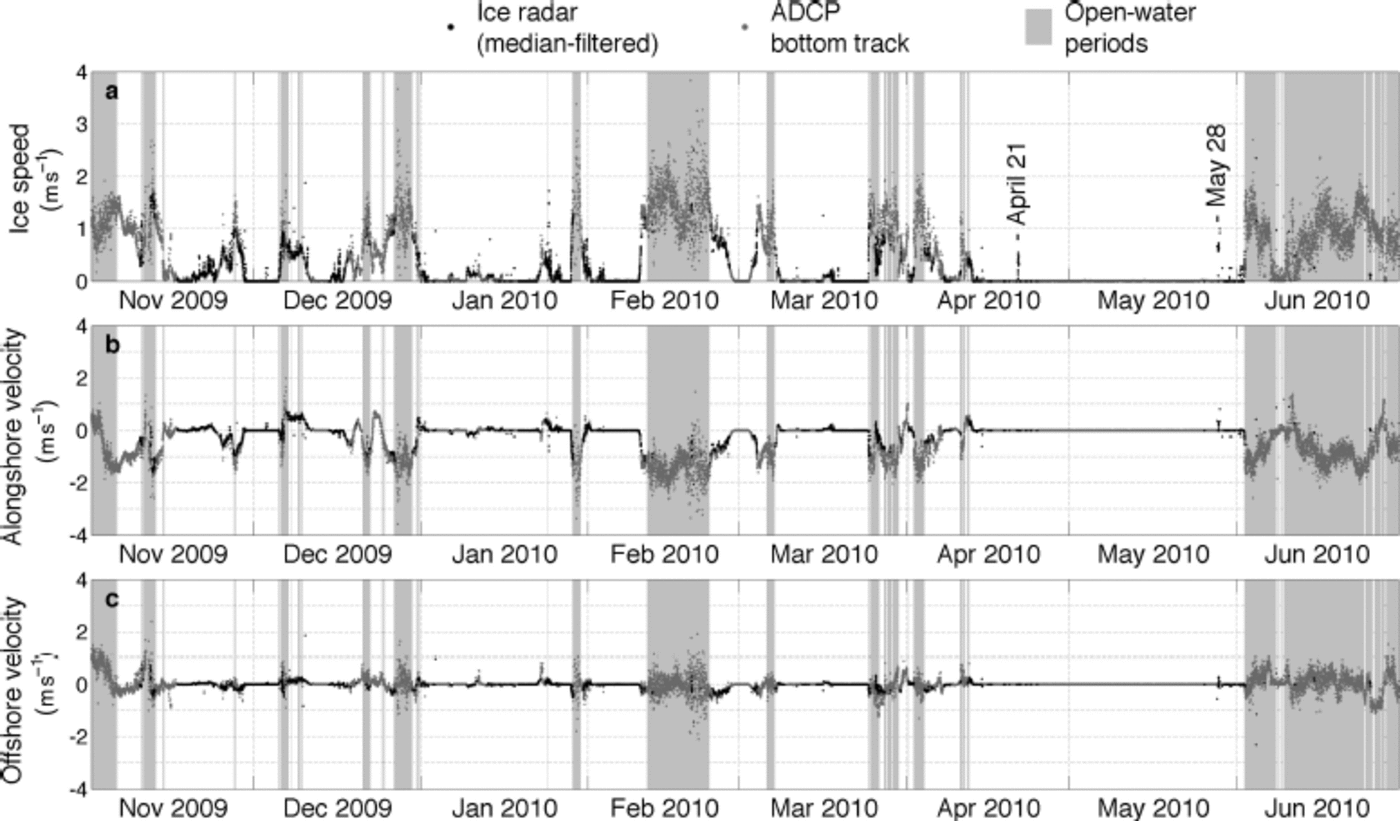
Examining the radar-derived ice velocities and ADCP bottom-tracked velocities as time series (Fig. 8) confirms the overall good agreement between these two independent observations of ice motion while also allowing closer scrutiny of those occasions when the results differ. The gray boxes indicate periods of open water inferred from the bottom track error as described above. It is clear that these periods correspond to the highest velocities and also coincide with many of the gaps in the coastal radar velocity record. Examination of the radar imagery during these data gaps reveals an absence of reflectors over the mooring site. We remind the reader that, due to the insensitivity of the coastal radar system to areas of smooth ice, the absence of reflectors in the imagery does not necessarily imply an absence of ice on the ocean, but in those cases where there is sufficient daylight we are able to confirm the presence of open water through examination of images from the Barrow sea-ice webcam (http://seaice.alaska.edu/gi/observatories/barrow_webcam), which is co-located with the radar. Despite the gaps in the radar velocity record, there are occasions when the radar was able to detect and track ice during periods of inferred open water. For these cases the overall rms difference between the bottom track data and median-filtered radar-derived ice velocity is 0.48 ms–¹with a tendency for the radar to underestimate the ice velocity relative to the ADCP.

Fig. 8.

Time series of (a) ice velocity magnitude and (b) alongshore and (c) offshore components derived from the ice radar (black dots) and ADCP bottom track data (gray dots). Open-water periods are shown by gray shading.

4.1. Reconciling thickness and draft measurements

To our knowledge, the AEM flight that twice passed within 350 m of mooring B2 allowed the first direct comparison between airborne and submarine measurements of ice thickness at a scale larger than that of an individual floe (e.g. Doble and others, 2011). To compare AEM and IPS data it is important to understand the measurements that each instrument makes and how these relate to each other. Primarily it is important to recall that the EM-bird measures the combined tpassed within 350 m of mooring B2 allowed the first direct comparison between airborne and submarine measurements of ice thickness at a scale larger than that of an individual floe (e.g. Reference Doble, Skouroup and WadhamsDoble and others, 2011). To compare AEM and IPS data it is important to understand the measurements that each instrument makes and how these relate to each other. Primarily it is important to recall that the EM-bird measures the combined thickness of snow and ice while the IPS measures just the draft of the ice. Rearranging Eqn (1) and substituting a thickness-weighted mean density of snow and ice, p ^*, we can express the expected relationship between the AEM and IPS measurements as

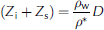
where

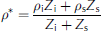
At the time of the AEM overpass, the temperature and salinity at mooring B2 were -1.686°C and 31.69, respectively, which yields a sea-water density, pw, of 1025 kgm^–3. Substituting this and the modal values derived from our measurements shown in Figure 6 (Zi +Z _s= 1.6±0.025 m and D= 1.35 ±0.025 m), we derive a value of p* of 860 ± 30 kgm ^{−– 3} . Assuming a sea-ice density of 9 1 0 ± 2 0 kgm^–3 (Reference Timco and FrederkingTimco and Frederking, 1996) and a snow density of 300 ± 100 kg m^–3taken from data for March reported by Reference WarrenWarren and others (1999), we can use Eqn (3) to estimate that the level ice in the vicinity of mooring B2 on 12 April 2010 was 1.48 ± 0.09 m thick, with a snow depth of 0.12 ± 0.09 m. Here we assume the uncertainties are normally distributed and uncorrelated, and we use the Gaussian method to propagate errors. Although the largest uncertainty, both in relative and absolute terms, is that for snow depth, the uncertainty in the value of ρ* has the biggest effect on the derived values. This in turn is dependent on the uncertainties in the densities of water and ice and our ability to determine the modes in the AEM and IPS data.

For comparison, sea ice at the UAF mass-balance site (Fig. 1) on 12 April was 1.24m thick and the snow depth measured by three sonic altimeters ranged between 0.29 and 0.43 m, with a mean of 0.35 m. Although these values are not in direct agreement, the differences in ice thickness and snow depth are consistent with each other. Although measurements of snow on drifting sea ice are rare, we expect snow to be thicker on landfast ice along the Alaska Chukchi Coast than on drifting ice offshore. Shorefast ice near Barrow is typically among the first ice to form in the Chukchi Sea and collects snow drifting in from a broad catchment carried by prevailing northeasterly winds. In contrast, these same prevailing winds create a semi-persistent coastal polynya at the seaward edge of the landfast ice (Reference Eicken, Shapiro, Gaylord and MahoneyEicken and others, 2006; Reference MahoneyMahoney and others, 2012) that may reduce the amount of snow advected onto drifting sea ice downwind. With less snow to insulate the ice surface, the offshore ice can therefore be expected to be thicker.

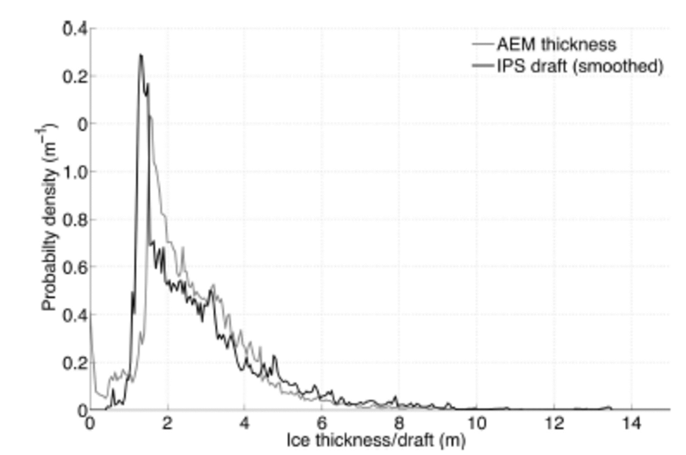
Closer examination of the two distributions (Fig. 6) shows that they differ not only in the position of their modes, but also in the shape of the tail, most noticeably for ice thicknesses less than 4 m. This difference cannot be accounted for by a simple isostatic assumption, so instead we consider the differing footprints of the two instruments. To better match the footprints of the two instruments, we applied a 70 m boxcar smoothing filter to the IPS data. This smoothing changes the shape of the tail of the IPS draft distribution to more closely resemble that of the AEM data (Fig. 9). A Gaussian filter was also tried, but resulted in a poorer fit. Having reconciled the sampling footprints of the IPS and AEM, we then applied a stretching to the smoothed IPS draft distribution that minimized the rms difference between it and the AEM distribution. Using this approach we find a conversion factor from ice draft to total thickness of 1.20 ± 0 . 0 1 m (Fig. 10), which corresponds to a distribution-wide mean value of ρ*of 850 ± 0 . 30 kg m^–3. Within 10 km of mooring B2, the mean thickness of ice and snow measured by the EM-bird is 2.66 m. Our mean value //therefore corresponds to a mean ice thickness of 2.40 ± 0 . 14 m and a mean snow depth of 0.26 ± 0 . 14 m.

Fig. 9.

Probability distribution of combined ice and snow thickness (AEM) and 70 m boxcar smoothed ice draft (IPS) derived from all measurements within 10 km of mooring B2.

Fig. 10.

Probability distribution of combined ice and snow thickness (AEM) and 70 m boxcar smoothed, isostatically adjusted ice draft (IPS*1.20) derived from all measurements within 10 km of mooring B2.

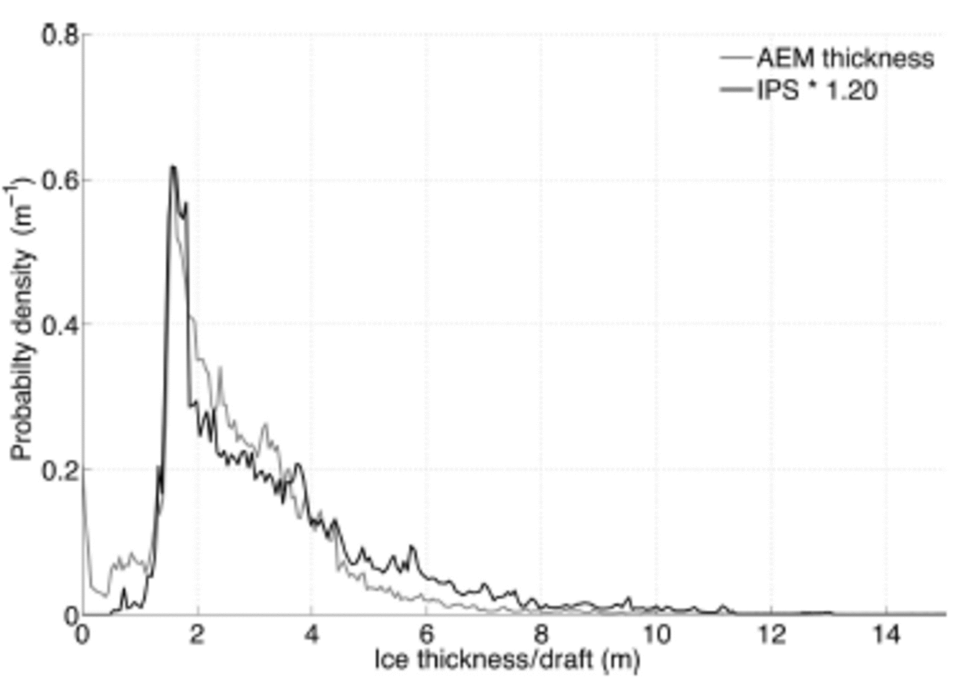
Although there is good agreement between the modes of the AEM and smoothed, shifted IPS (Fig. 10), there are differences in the two distributions that warrant further comment. We expect the distributions to differ simply because the AEM flight path and IPS pseudo-track do not overlap and the two sensors did not observe exactly the same ice. We believe this explains why the AEM data show a greater amount of thin ice (<1 m) than the IPS data. There are also differences in the tail such that the AEM data indicate more ice between 1.4 and 4.0 m, and less ice >4 m, than the IPS data. This may derive from the different sampling areas, but it also probably indicates that deformed ice must be treated differently than level ice when it comes to assumptions concerning the effective mean ice density or electrical conductivity. This is discussed further in Section 5. The relative over- and under-observation of ice thinner and thicker than ∼4 m, respectively, might also be explained if the sensitivity of the EM-bird was reduced to the noise level of the receiver at this equivalent range. However, theoretical considerations of the EM response show that signal-to-noise ratios are not critical until a range of 30–35 m, corresponding to an ice thickness of 15–20m at a survey altitude of 15 m.

4.2. Coastal ice motion observed from above and below

Figure 8 shows the variability of ice motion at one point in the coastal zone near Barrow over a full ice season. Zero ice motion indicates the ice above the mooring was landfast. The record shows landfast ice forming over the mooring as early as mid-November, with several attachment and detachment events occurring throughout the year. In general, the periods of landfast ice lengthen over the course of the year before final break-up over the mooring around the beginning of June. Both the ADCP and the coastal radar system identify each cessation and recommencement of ice motion, though in some cases the occurrence of landfast ice coincides with data gaps in the radar-derived ice velocity record (e.g. the latter part of April and most of May). Examination of the radar imagery on these occasions indicates these gaps are due to a lack of reflectors over the mooring. However, the presence of ice can be confirmed from the presence of stationary reflectors in the neighborhood. On other occasions, the radar data show apparent ice motion while the ADCP data continue to indicate landfast ice (e.g. 21 April and 28 May). In these cases we find that the ice motion algorithm was confused by the passage of snow squalls and migrating birds.

In identifying the onset of ice motion at the end of land-fast periods, the ADCP and radar-derived ice velocity records provide accurate timings of detachment events. The detachment of landfast ice represents a significant hazard to anyone on the ice when it begins to move. At the same time, such events are important to communities along the Alaska Chukchi Coast during the spring whaling season, since any open water created provides access to hunt the whales migrating north along the coast (Reference George, Huntington, Brewster, Eicken and GlennGeorge and others, 2004; Reference Druckenmiller, Eicken, Brower, Krupnik, Aporta and GearheardDruckenmiller and others, 2010). Previous studies of coastal ice dynamics using surface radars have noted that it may be possible to detect precursor events leading up to detachments. Reference Shapiro and MetznerShapiro and Metzner (1989) and Reference Mahoney, Eicken and ShapiroMahoney and others (2007) report the occurrence of ‘flickering’ in the radar imagery prior to breakout events. Reference Rohith, Jones, Eicken and KambhamettuRohith and others (2013) have taken this further to develop an algorithm based on Hidden Markov Models that has successfully detected some breakout events based on ‘hidden’ characteristics of the gridded flow field. A more detailed study of landfast ice detachments, including an analysis of ice deformation from radar-derived gridded ice velocities, is provided by Reference JonesJones (2013).