


1. Introduction
Dynamic stall happens when the angle of attack of an aerofoil exceeds its critical stall angle, due to either unsteady aerofoil motions or variations in flow conditions, such as gust encounters (McCroskey Reference McCroskey1981; Jones & Cetiner Reference Jones and Cetiner2021). The dynamic stall phenomenon is commonly observed on the retreating blades of helicopter rotors in forward flight, horizontal- and vertical-axis wind turbines, cross-flow hydro-turbines and micro-aerial vehicles (Buchner et al. Reference Buchner, Soria, Honnery and Smits2018; Le Fouest & Mulleners Reference Le Fouest and Mulleners2022; Santos Pereira Reference Santos Pereira2022; Dave & Franck Reference Dave and Franck2023). A typical dynamic stall cycle includes attached flow, the emergence and spreading of flow reversal on the aerofoil suction side, the formation of a large-scale dynamic stall vortex, the separation of the first dynamic stall vortex initiating full stall, massive flow separation, and eventually flow reattachment (Carr, McAlister & McCroskey Reference Carr, McAlister and McCroskey1977; Shih et al. Reference Shih, Lourenco, Van Dommelen and Krothapalli1992; Mulleners & Raffel Reference Mulleners and Raffel2013). Dynamic stall is affected by the aerofoil geometry, the wing kinematics, and flow conditions (Choudhry et al. Reference Choudhry, Leknys, Arjomandi and Kelso2014; Corke & Thomas Reference Corke and Thomas2015; Visbal & Garmann Reference Visbal and Garmann2018). The aerofoil geometry mainly affects the stall onset and hysteresis loops. Thicker aerofoils generally stall at higher angles of attack and have larger hysteresis loops than thinner aerofoils.
The stall onset and flow recovery are delayed in dynamic stall compared to classic static aerofoil separation and reattachment (Carr et al. Reference Carr, McAlister and McCroskey1977; Shih et al. Reference Shih, Lourenco, Van Dommelen and Krothapalli1992; Le Fouest et al. Reference Le Fouest, Deparday and Mulleners2021). The separation delay is well-characterised using the non-dimensional measure of the kinematic unsteadiness defined as the non-dimensional pitch rate (Mulleners & Raffel Reference Mulleners and Raffel2012; Ayancik & Mulleners Reference Ayancik and Mulleners2022; Kiefer et al. Reference Kiefer, Brunner, Hansen and Hultmark2022). The delay in stall onset increases the maximum attainable lift, as the lift continues to grow with increasing angle of attack during stall development. Although the initial stall delay and lift overshoot may seem advantageous, they lead to large, unsteady aerodynamic loads that reduce efficiency, introduce strong vibrations, and increase structural stress.
Due to the adverse effects of dynamic stall onset, this phase has historically received more attention than stall recovery (Sheng, Galbraith & Coton Reference Sheng, Galbraith and Coton2008; Mulleners & Raffel Reference Mulleners and Raffel2012; Morris & Rusak Reference Morris and Rusak2013), and the developed dynamic stall models typically predict separation onset more accurately than the recovery onset (Sheng et al. Reference Sheng, Galbraith and Coton2008; Ayancik & Mulleners Reference Ayancik and Mulleners2022; Damiola et al. Reference Damiola, Decuyper, Runacres and De Troyer2024a ). A more profound understanding of the reattachment process is essential to improve the modelling of the overall aerodynamic performance, and to develop strategies for gust exits and to alleviate dynamic hysteresis. The hysteresis arises directly from the stall onset and recovery delays, and the amount of hysteresis is influenced by factors such as the degree of flow separation, the reduced frequency of the pitching motion, and the presence of a strong dynamic stall vortex (Ekaterinaris & Platzer Reference Ekaterinaris and Platzer1998; Williams et al. Reference Williams, An, Iliev, King and Reißner2015). In the context of gust-induced flow separation, considerable research has focused on exploring the aerodynamic response of wings to gusts, developing mitigation strategies, and modelling the aerodynamic performance of wings (Perrotta & Jones Reference Perrotta and Jones2017; Sedky, Lagor & Jones Reference Sedky, Lagor and Jones2020; Jones & Cetiner Reference Jones and Cetiner2021). Resulting gust-response models and control strategies yield better results during gust entry than during the gust exit (Andreu-Angulo & Babinsky Reference Andreu-Angulo and Babinsky2023; Gementzopoulos, Sedky & Jones Reference Gementzopoulos, Sedky and Jones2024).
Among the first researchers to systematically study the unsteady flow reattachment process on aerofoils were Niven, Galbraith & Herring (Reference Niven, Galbraith and Herring1989). They considered experimental data from various aerofoils undergoing ramp-down motions conducted in the facilities of Glasgow University. The results of these experimental campaigns were collected into the University of Glasgow’s aerofoil database (Galbraith, Gracey & Leitch Reference Galbraith, Gracey and Leitch1992). These early studies found that flow reattachment is always initiated at an angle of attack close to the static stall, and progresses from the leading edge towards the trailing edge (Niven et al. Reference Niven, Galbraith and Herring1989; Galbraith et al. Reference Galbraith, Gracey and Leitch1992). Green & Galbraith (Reference Green and Galbraith1995) were the first to identify a ramp-down wave travelling from the leading edge to the trailing edge as an essential part of the recovery process. Through smoke flow visualisation, the ramp-down wave was observed to convect excess wake fluid past the aerofoil, which is an essential precursor for actual boundary layer reattachment. The footprint of the ramp-down wave in the surface pressure data is a local ridge indicating a negative rate of change in suction that travels from the leading to the trailing edge. The travelling speed of the ramp-down wave is independent of the reduced pitch rate and aerofoil profile, and is significantly faster than the actual reattachment. The actual reattachment is indicated by the local recovery of suction, which moves with a rate that strongly depends on the pitch rate.
The reattachment process on periodically pitching aerofoils is more complicated than in simple ramp-down motions due to the influence of the strong transient vortex shedding in the near wake. The issue was tackled by Ahmed & Chandrasekhara (Reference Ahmed and Chandrasekhara1994) for a large-amplitude sinusoidal pitching motion based on flow field visualisation. Quantitative velocity and density field information was obtained using laser Doppler velocimetry and point diffraction interferometry. Reattachment was again found to begin near the static stall angle of attack, but the pointwise character of the laser Doppler velocimetry technique did not allow for a deeper insight into the process itself. In this paper, we revisit the reattachment of dynamically stalled flows on oscillating aerofoils. We combine flow field measurements from time-resolved particle image velocimetry (PIV) with surface pressure measurements from a thin aerofoil in deep stall conditions.
From the surface pressure data, we can extract the leading-edge suction parameter, which quantifies the suction force at an aerofoil leading edge. The leading-edge suction parameter is a reliable indicator of the onset and evolution of dynamic stall (Ramesh et al. Reference Ramesh, Gopalarathnam, Edwards, Ol and Granlund2013, Reference Ramesh, Gopalarathnam, Granlund, Ol and Edwards2014; Deparday & Mulleners Reference Deparday and Mulleners2019; Miotto et al. Reference Miotto, Wolf, Gaitonde and Visbal2022). For a given aerofoil shape and Reynolds number, there is a critical threshold beyond which leading-edge vortex formation initiates (Ramesh et al. Reference Ramesh, Granlund, Ol, Gopalarathnam and Edwards2018). The critical leading-edge suction parameter value remains largely independent of the motion kinematics, except when high degrees of trailing-edge flow separation are present. Between the start of the formation and the shedding of the leading-edge vortex, the leading-edge suction parameter increases beyond its critical value. The maximum leading-edge suction parameter increases with increasing pitch rate of the motion, and sharply drops to near-zero values after leading-edge flow separation occurs (Deparday & Mulleners Reference Deparday and Mulleners2019; Narsipur et al. Reference Narsipur, Hosangadi, Gopalarathnam and Edwards2020; Sudharsan, Narsipur & Sharma Reference Sudharsan, Narsipur and Sharma2023). The leading-edge suction parameter effectively captures the events at the very leading edge, and it is less sensitive to post-stall vortex shedding events occurring away from the leading edge (Sudharsan & Sharma Reference Sudharsan and Sharma2024). As dynamic stall reattachment starts from the leading edge, the leading-edge suction parameter has the potential to be an insightful quantity that we analyse in this paper as part of our revisit of dynamic stall reattachment.
2. Experimental material and methods
Wind tunnel experiments were conducted to investigate the dynamic stall life cycle on a constantly pitching aerofoil in a uniform flow at a free-stream Reynolds number $\textit{Re}={9.2\times {10}^{5}}$
based on the chord length
$\textit{Re}={9.2\times {10}^{5}}$
based on the chord length $c$
(Mach number
$c$
(Mach number $\textit{Ma}={0.14}$
). The experiments were conducted in the closed-circuit, low-speed wind tunnel at the German Aerospace Centre (DLR) in Göttingen. The wind tunnel had an open test section of length 1.3 m and a rectangular nozzle measuring
$\textit{Ma}={0.14}$
). The experiments were conducted in the closed-circuit, low-speed wind tunnel at the German Aerospace Centre (DLR) in Göttingen. The wind tunnel had an open test section of length 1.3 m and a rectangular nozzle measuring $0.75\,\textrm {m}\times 1.05\,\textrm {m}$
.
$0.75\,\textrm {m}\times 1.05\,\textrm {m}$
.
A two-dimensional aerofoil model with an OA209 profile was used for the experiments. The aerofoil had maximum thickness to chord ratio ${9}{\,\%}$
, chord length 0.3 m, and aspect ratio 5. The static stall angle of this aerofoil under the given experimental conditions was
${9}{\,\%}$
, chord length 0.3 m, and aspect ratio 5. The static stall angle of this aerofoil under the given experimental conditions was ${\alpha }_{\textit{ss}}={21.4^\circ }$
, and was determined from a static polar (Mulleners & Raffel Reference Mulleners and Raffel2012). The aerofoil was subjected to a sinusoidally oscillating motion about its quarter-chord axis with mean incidence
${\alpha }_{\textit{ss}}={21.4^\circ }$
, and was determined from a static polar (Mulleners & Raffel Reference Mulleners and Raffel2012). The aerofoil was subjected to a sinusoidally oscillating motion about its quarter-chord axis with mean incidence ${\alpha }_{0}$
, amplitude
${\alpha }_{0}$
, amplitude ${\alpha }_{1}$
, and oscillation frequency
${\alpha }_{1}$
, and oscillation frequency ${f}_{osc}$
. The latter is preferably written in dimensionless form as the reduced frequency
${f}_{osc}$
. The latter is preferably written in dimensionless form as the reduced frequency $k=\pi \,{f}_{osc}\,c/{{{U}}}_{\infty }$
, where
$k=\pi \,{f}_{osc}\,c/{{{U}}}_{\infty }$
, where ${{{U}}}_{\infty }$
is the free-stream velocity. The mean incidence, amplitude and reduced frequency were varied such that
${{{U}}}_{\infty }$
is the free-stream velocity. The mean incidence, amplitude and reduced frequency were varied such that ${\alpha }_{0} \in \{{18}^{\circ }, {20}^{\circ }, {22}^{\circ }\}$
,
${\alpha }_{0} \in \{{18}^{\circ }, {20}^{\circ }, {22}^{\circ }\}$
, ${\alpha }_{1} \in \{{6}^{\circ }, {8}^{\circ }\}$
and
${\alpha }_{1} \in \{{6}^{\circ }, {8}^{\circ }\}$
and $k \in \{{0.050}, {0.075}, {0.10}\}$
. In this study, we focus only on cases that resulted in deep dynamics stall, which according to Mulleners & Raffel (Reference Mulleners and Raffel2012) are cases where dynamic stall occurs before the aerofoil reaches the maximum angle of attack. The data have been used in previous studies (Mulleners & Raffel Reference Mulleners and Raffel2012, Reference Mulleners and Raffel2013; Ansell & Mulleners Reference Ansell and Mulleners2019; Deparday & Mulleners Reference Deparday and Mulleners2019; Ayancik & Mulleners Reference Ayancik and Mulleners2022).
$k \in \{{0.050}, {0.075}, {0.10}\}$
. In this study, we focus only on cases that resulted in deep dynamics stall, which according to Mulleners & Raffel (Reference Mulleners and Raffel2012) are cases where dynamic stall occurs before the aerofoil reaches the maximum angle of attack. The data have been used in previous studies (Mulleners & Raffel Reference Mulleners and Raffel2012, Reference Mulleners and Raffel2013; Ansell & Mulleners Reference Ansell and Mulleners2019; Deparday & Mulleners Reference Deparday and Mulleners2019; Ayancik & Mulleners Reference Ayancik and Mulleners2022).
The surface pressure distribution was recorded using 41 differential pressure transducers (type Kulite XCQ-093) mounted along the central cross-sectional plane of the aerofoil (see Mulleners & Raffel (Reference Mulleners and Raffel2013) or figure 12 for the locations of the pressure sensors). The pressure data were sampled at rate 6 kHz for duration 15 s, which corresponds to approximately 80 cycles for the highest pitching frequency, and 40 for the lowest frequency. The aerofoil surface pressure distributions were integrated to obtain the lift and moment coefficients. The leading-edge suction parameter is evaluated following the procedure explained in Deparday & Mulleners (Reference Deparday and Mulleners2019). The procedure involves determining the leading-edge suction vector by integrating pressure data from 13 unsteady pressure sensors positioned within the front 10 % of the aerofoil. The experimental leading-edge suction parameter ${A}_{0}$
is then obtained by projecting the leading-edge suction vector along the chordwise direction, following the approach of Katz & Plotkin (Reference Katz and Plotkin2001).
${A}_{0}$
is then obtained by projecting the leading-edge suction vector along the chordwise direction, following the approach of Katz & Plotkin (Reference Katz and Plotkin2001).
Stereoscopic time-resolved PIV (TR-PIV) was conducted in the cross-sectional plane at the model mid-span. The TR-PIV system consisted of a diode-pumped Nd:YAG laser (Lee Laser, LDP- $200$
MQG Dual) that emitted laser pulses with energy approximately 10 mJ per pulse at 3 kHz, and two CMOS cameras (Photron Ultima APX-RS). The vertical plane at model mid-span was illuminated by the laser from above, and the cameras were mounted in a stereoscopic set-up alongside the wind tunnel diffuser. The width of the field of view covered the entire chord for the relevant angle of attack range. Time series of 3072 image pairs at full camera resolution (
$200$
MQG Dual) that emitted laser pulses with energy approximately 10 mJ per pulse at 3 kHz, and two CMOS cameras (Photron Ultima APX-RS). The vertical plane at model mid-span was illuminated by the laser from above, and the cameras were mounted in a stereoscopic set-up alongside the wind tunnel diffuser. The width of the field of view covered the entire chord for the relevant angle of attack range. Time series of 3072 image pairs at full camera resolution ( $1024\,\textrm {px}\times 1024\,\textrm {px}$
) were recorded at 1500 Hz. The time delay between the laser pulses in the image pairs was
$1024\,\textrm {px}\times 1024\,\textrm {px}$
) were recorded at 1500 Hz. The time delay between the laser pulses in the image pairs was ${30}{\unicode{x03BC} \textrm {m}}$
. The camera buffers allowed us to record images for 2 s, covering five full oscillation cycles for the lowest pitching frequency, and up to ten cycles for the highest frequency. After mapping the views of both cameras, the dimensions of the PIV measurement window were
${30}{\unicode{x03BC} \textrm {m}}$
. The camera buffers allowed us to record images for 2 s, covering five full oscillation cycles for the lowest pitching frequency, and up to ten cycles for the highest frequency. After mapping the views of both cameras, the dimensions of the PIV measurement window were $335\,\textrm{mm}\times 165\,\textrm{mm}$
, with spatial resolution
$335\,\textrm{mm}\times 165\,\textrm{mm}$
, with spatial resolution ${5.0}\,\textrm{px}\,\textrm{mm}^{-1}$
. The PIV images were processed using interrogation window size
${5.0}\,\textrm{px}\,\textrm{mm}^{-1}$
. The PIV images were processed using interrogation window size $32\,\textrm{px}\times 32\,\textrm{px}$
and overlap approximately 80 %, yielding grid spacing 6 px or 1.2 mm, which is less than
$32\,\textrm{px}\times 32\,\textrm{px}$
and overlap approximately 80 %, yielding grid spacing 6 px or 1.2 mm, which is less than $0.005 c$
. The interrogation window size was minimised, ensuring an acceptable signal-to-noise ratio. The window overlap, on the other hand, was maximised to avoid artificial smoothing of velocity gradients (Richard et al. Reference Richard, Bosbach, Henning, Raffel, Willert and van der Wall2006). The velocity fields were rotated into the aerofoil reference system with the
$0.005 c$
. The interrogation window size was minimised, ensuring an acceptable signal-to-noise ratio. The window overlap, on the other hand, was maximised to avoid artificial smoothing of velocity gradients (Richard et al. Reference Richard, Bosbach, Henning, Raffel, Willert and van der Wall2006). The velocity fields were rotated into the aerofoil reference system with the $x$
-axis along the chord, the
$x$
-axis along the chord, the $y$
-axis along the span, and the
$y$
-axis along the span, and the $z$
-axis upwards, perpendicular to the chord. The origin is located at the rotation axis at the aerofoil quarter-chord axis. Simultaneously to the TR-PIV, the surface pressure distribution at the model mid-span was scanned at approximately 6 kHz for approximately 15 s. The data acquisition was synchronised with the recording of the PIV images, allowing for straightforward assignment of the instantaneous pressure distributions to each of the acquired velocity fields. Additional details about the experimental set-up and measurements can be found in Mulleners (Reference Mulleners2010) and Mulleners & Raffel (Reference Mulleners and Raffel2012, Reference Mulleners and Raffel2013).
$z$
-axis upwards, perpendicular to the chord. The origin is located at the rotation axis at the aerofoil quarter-chord axis. Simultaneously to the TR-PIV, the surface pressure distribution at the model mid-span was scanned at approximately 6 kHz for approximately 15 s. The data acquisition was synchronised with the recording of the PIV images, allowing for straightforward assignment of the instantaneous pressure distributions to each of the acquired velocity fields. Additional details about the experimental set-up and measurements can be found in Mulleners (Reference Mulleners2010) and Mulleners & Raffel (Reference Mulleners and Raffel2012, Reference Mulleners and Raffel2013).
The finite-time Lyapunov exponent (FTLE) is calculated using the time-resolved flow field data to extract and analyse separation and reattachment lines, and to identify Lagrangian coherent flow structures (Green, Rowley & Smits Reference Green, Rowley and Smits2011). The velocity field is artificially seeded and integrated backwards in time to obtain negative FTLE (nFTLE) ridges, and forwards in time to obtain the positive FTLE (pFTLE) ridges. The backward integration is similar to using smoke visualisation, and shows where the particles come from. The nFTLE ridges indicate regions where nearby flow particles experience the highest attraction, such as near separation lines, and the pFTLE ridges indicate regions where nearby flow particles are repelled (Haller Reference Haller2002; Shadden, Lekien & Marsden Reference Shadden, Lekien and Marsden2005). The intersection of nFTLE and pFTLE ridges indicates the location of a saddle point. Monitoring the emergence and trajectories of saddle points provides insights into the timing and location of vortex formation, and can help in understanding flow separation and attachment (Mulleners & Raffel Reference Mulleners and Raffel2012; Rockwood, Huang & Green Reference Rockwood, Huang and Green2018; Kissing et al. Reference Kissing, Kriegseis, Li, Feng, Hussong and Tropea2020).
3. Results
Here, we revisit the reattachment process of a thin aerofoil undergoing deep dynamic stall based on time-resolved pressure and velocity field measurements. First, we revise the overall characteristics of dynamic stall by the example of a selected representative pitching cycle. Then we focus on the flow development during reattachment, identify successive reattachment stages, and analyse the corresponding characteristic surface footprints. Finally, we establish a critical condition for the onset of stall recovery, and quantify how the time scales associated with the different reattachment stages evolve as a function of the effective unsteadiness of the pitching motion. A representative cycle is used for the detailed discussion, and the analysis is then extended to multiple cycles of various pitching kinematics that all lead to deep stall.
Spatio-temporal evolution of (a) the pressure coefficient on the airfoil suction side from the leading-edge (LE) to the trailing-edge (TE) and (b) the temporal evolution of the lift coefficient for a selected pitching cycle indicated by the solid black line ( ${\alpha }_{0}={20}^{\circ }$
,
${\alpha }_{0}={20}^{\circ }$
, ${\alpha }_{1}={8}^{\circ }$
,
${\alpha }_{1}={8}^{\circ }$
, $k={0.05}$
,
$k={0.05}$
, ${\dot {\alpha }}_{\textit{ss}}={0.0135}$
). The shaded grey bands in the lift evolution represent the area between the minimum and maximum envelopes obtained from 39 recorded cycles. The thick dashed orange line shows the quasi-static evolution of the lift coefficient
${\dot {\alpha }}_{\textit{ss}}={0.0135}$
). The shaded grey bands in the lift evolution represent the area between the minimum and maximum envelopes obtained from 39 recorded cycles. The thick dashed orange line shows the quasi-static evolution of the lift coefficient ${C}_{l,{qs}}$
. Vertical dashed lines indicate the moment when the static stall angle is exceeded during pitch-up (
${C}_{l,{qs}}$
. Vertical dashed lines indicate the moment when the static stall angle is exceeded during pitch-up ( ${t}_{ss \nearrow }$
) and the moment when the angle of attack falls below the static stall angle during pitch-down (
${t}_{ss \nearrow }$
) and the moment when the angle of attack falls below the static stall angle during pitch-down ( ${t}_{ss \searrow }$
). The extra axis on top indicates the angle of attack variation for the cycle. The extra axis below indicates the non-dimensional time variation shifted based on the instant when the geometric angle of attack falls below the critical static stall angle during the pitch-down motion (
${t}_{ss \searrow }$
). The extra axis on top indicates the angle of attack variation for the cycle. The extra axis below indicates the non-dimensional time variation shifted based on the instant when the geometric angle of attack falls below the critical static stall angle during the pitch-down motion ( ${t}_{ss \searrow }$
).
${t}_{ss \searrow }$
).

3.1. Footprints of dynamic stall
The typical surface pressure and force response of a single representative cycle of a continuously sinusoidally pitching aerofoil undergoing deep dynamic stall is presented in figure 1. The data were obtained by oscillating the aerofoil around mean angle ${\alpha }_{0}={20}^{\circ }$
, with amplitude
${\alpha }_{0}={20}^{\circ }$
, with amplitude ${\alpha }_{1}={8}^{\circ }$
, and reduced frequency
${\alpha }_{1}={8}^{\circ }$
, and reduced frequency $k={0.05}$
. We take the start of the cycle at the moment when the aerofoil angle of attack is lowest and the pitch-up motion begins. Additional cycles of the lift response are presented in figure 9 in Appendix A.
$k={0.05}$
. We take the start of the cycle at the moment when the aerofoil angle of attack is lowest and the pitch-up motion begins. Additional cycles of the lift response are presented in figure 9 in Appendix A.
At the beginning of the cycle, the flow is attached and the lift coefficient increases with the angle of attack, which is primarily due to an increase in the leading-edge suction (figure 1 a). The measured lift coefficient follows the quasi-static lift response prediction for an aerofoil pitching around the quarter-chord axis:
 \begin{align}{C}_{l,{qs}}(t) &= {C}_{l,\textit{static}}(\alpha (t)) + 2\pi \frac {\dot {\alpha }(t)\,c}{2{{{U}}}_{\infty }}\nonumber\\& = {C}_{l,\textit{static}}(\alpha (t)) + 2\pi\, \Delta \alpha (t),\end{align}
with ${C}_{l,\textit{static}}(\alpha (t))$
the linear extrapolation of the static lift response for attached flow, and
${C}_{l,\textit{static}}(\alpha (t))$
the linear extrapolation of the static lift response for attached flow, and $\dot {\alpha }(t)$
the instantaneous pitch rate (figure 1
b). The contribution of the unsteady pitching motion to the lift can also be expressed as the result of a variation in the effective angle of attack
$\dot {\alpha }(t)$
the instantaneous pitch rate (figure 1
b). The contribution of the unsteady pitching motion to the lift can also be expressed as the result of a variation in the effective angle of attack ${\alpha }_{\textit{eff}}$
, by
${\alpha }_{\textit{eff}}$
, by $\Delta \alpha ={\alpha }_{\textit{eff}}-\alpha$
(see Appendix B). When the aerofoil is pitching up, the effective angle of attack is increased by
$\Delta \alpha ={\alpha }_{\textit{eff}}-\alpha$
(see Appendix B). When the aerofoil is pitching up, the effective angle of attack is increased by $\dot {\alpha }(t)\,c/(2{{{U}}}_{\infty })$
, and we expect an increase in the lift coefficient compared to the static lift response if the flow is attached. When the aerofoil is pitching down, the effective angle of attack is decreased by
$\dot {\alpha }(t)\,c/(2{{{U}}}_{\infty })$
, and we expect an increase in the lift coefficient compared to the static lift response if the flow is attached. When the aerofoil is pitching down, the effective angle of attack is decreased by $\dot {\alpha }(t)c/(2{{{U}}}_{\infty })$
. As the variations
$\dot {\alpha }(t)c/(2{{{U}}}_{\infty })$
. As the variations $\Delta \alpha$
will be typically less than
$\Delta \alpha$
will be typically less than ${1.6}^{\circ }$
for the kinematics considered here (Appendix B), we use the geometric angle of attack as our reference.
${1.6}^{\circ }$
for the kinematics considered here (Appendix B), we use the geometric angle of attack as our reference.
For the example pitching motion presented in figure 1, the static stall angle of attack is reached at $t/T=0.28$
, but the leading-edge suction and the lift coefficient continue to increase until
$t/T=0.28$
, but the leading-edge suction and the lift coefficient continue to increase until $t/T=0.40$
, when dynamic stall occurs. The onset of dynamic stall is defined as the detachment of the primary stall vortex, which coincides with a decrease in lift and the breakdown of the leading-edge suction. The detachment of the stall vortex is marked by the emergence of a saddle point near the leading edge (Mulleners & Raffel Reference Mulleners and Raffel2012). The onset of dynamic stall is indicated by the axis label
$t/T=0.40$
, when dynamic stall occurs. The onset of dynamic stall is defined as the detachment of the primary stall vortex, which coincides with a decrease in lift and the breakdown of the leading-edge suction. The detachment of the stall vortex is marked by the emergence of a saddle point near the leading edge (Mulleners & Raffel Reference Mulleners and Raffel2012). The onset of dynamic stall is indicated by the axis label ${t}_{ds}$
in figure 1 and occurs after the static stall angle is exceeded, but before the maximum angle of attack is reached at
${t}_{ds}$
in figure 1 and occurs after the static stall angle is exceeded, but before the maximum angle of attack is reached at $t/T=0.5$
, classifying this case as a typical deep stall case. The delayed onset of stall and the associated lift overshoot are key features of dynamic stall. The onset and development of dynamic stall during the pitch-up half of the cycle have been discussed in detail in previous work based on the data set used in this paper (Mulleners & Raffel Reference Mulleners and Raffel2012, Reference Mulleners and Raffel2013; Ansell & Mulleners Reference Ansell and Mulleners2019; Deparday & Mulleners Reference Deparday and Mulleners2019).
$t/T=0.5$
, classifying this case as a typical deep stall case. The delayed onset of stall and the associated lift overshoot are key features of dynamic stall. The onset and development of dynamic stall during the pitch-up half of the cycle have been discussed in detail in previous work based on the data set used in this paper (Mulleners & Raffel Reference Mulleners and Raffel2012, Reference Mulleners and Raffel2013; Ansell & Mulleners Reference Ansell and Mulleners2019; Deparday & Mulleners Reference Deparday and Mulleners2019).
From here on, we focus on the post-stall behaviour and the stall reattachment process. A distinct post-stall feature in the space–time representation of the surface pressure distribution is the footprint of the primary dynamic stall vortex in the form of a local minimum pressure trace (figure 1
a). This low-pressure trace originates at the leading edge after dynamic stall onset, and moves towards the trailing edge for $t/T={0.40}{-}{0.50}$
. Interestingly, the chordwise location of the local pressure minimum corresponds not to the core of the dynamic stall vortex, but to the upstream saddle point that marks the separation of the stall vortex from the feeding shear layer (figure 2). Similar behaviour was observed by Rockwood et al. (Reference Rockwood, Huang and Green2018) for the flow around a circular cylinder. The location of the saddle point was determined as the intersection of the nFTLE and pFTLE ridges.
$t/T={0.40}{-}{0.50}$
. Interestingly, the chordwise location of the local pressure minimum corresponds not to the core of the dynamic stall vortex, but to the upstream saddle point that marks the separation of the stall vortex from the feeding shear layer (figure 2). Similar behaviour was observed by Rockwood et al. (Reference Rockwood, Huang and Green2018) for the flow around a circular cylinder. The location of the saddle point was determined as the intersection of the nFTLE and pFTLE ridges.
Combined visualisation of the instantaneous chordwise surface pressure distribution on the suction side, and the nFTLE and pFTLE ridges, for three selected time instants immediately following dynamic stall onset for the sinusoidal pitching motion presented in figure 1: (a) $\alpha ={27.2}^{\circ }$
, (b)
$\alpha ={27.2}^{\circ }$
, (b) $\alpha ={27.3}^{\circ }$
, (c)
$\alpha ={27.3}^{\circ }$
, (c) $\alpha ={27.4}^{\circ }$
. The pressure distribution is visualised by arrows normal to the surface, where the length of an arrow indicates the magnitude of the pressure coefficient. Only negative pressure coefficients are displayed. The intersection of the nFTLE (red) and pFTLE (blue) ridges indicates the location of a saddle point.
$\alpha ={27.4}^{\circ }$
. The pressure distribution is visualised by arrows normal to the surface, where the length of an arrow indicates the magnitude of the pressure coefficient. Only negative pressure coefficients are displayed. The intersection of the nFTLE (red) and pFTLE (blue) ridges indicates the location of a saddle point.

Dynamic stall onset marks the start of the fully stalled stage of the dynamic stall cycle, which is characterised by the repeated formation and shedding of large-scale coherent stall vortices. This post-stall vortex shedding creates additional low-pressure traces in the space–time representation of the surface pressure distribution and oscillations in the evolution of the instantaneous lift coefficient. The surface pressure traces and lift oscillations emerge approximately every 4–5 convective times, where the convective time is defined as ${t}_{c}={{{U}}}_{\infty }/c$
. This convective time interval corresponds to Strouhal number (
${t}_{c}={{{U}}}_{\infty }/c$
. This convective time interval corresponds to Strouhal number ( $St=\textit{fc}/{{{U}}}_{\infty }$
, with
$St=\textit{fc}/{{{U}}}_{\infty }$
, with $f$
the reciprocal of the dimensional time interval) 0.20–0.25 (figure 1).
$f$
the reciprocal of the dimensional time interval) 0.20–0.25 (figure 1).
Subtle variations in the timing of the post-stall vortex shedding can lead to cycle-to-cycle variations during full stall. The most prominent factors contributing to these variations include boundary layer and shear layer instabilities, the three-dimensionality of the stall cell, fluid–structure interactions leading to vibrations of the aerofoil, and free-stream turbulence or other perturbations in the free-stream velocity (Harms, Nikoueeyan & Naughton Reference Harms, Nikoueeyan and Naughton2018; Snortland et al. Reference Snortland, Scherl, Polagye and Williams2023; Damiola et al. Reference Damiola, Runacres and De Troyer2024b ). The degree of cycle-to-cycle variations during full stall is indicated by the shaded areas in the lift evolution in figure 1(b), which shows the range between the minimum and maximum envelopes for the recorded cycles. The aerodynamic load fluctuations can introduce structural vibrations and lead to premature fatigue failure of wings and blades. Despite their significant impact, post-stall load variations have not always been treated with the proper level of diligence, as they are often concealed by phase averaging (figure 1 b).
The cycle-to-cycle variations are not only prominent during the fully stalled stage, but are still present when the lift coefficient starts to recover to its quasi-static value (between $t/T\approx 0.8$
and
$t/T\approx 0.8$
and $t/T\approx 0.9$
in figure 1
b). Shortly before the lift coefficient recovers, the pressure coefficient near the leading edge becomes negative again, indicating leading-edge suction recovery (figure 1). The suction recovery onset coincides with the global minimum of the lift coefficient, after which the lift coefficient gradually recovers to its quasi-static value (figure 1). The recovery of the leading-edge suction and lift coefficient is delayed to angles of attack well below the static stall angle of attack, which leads to the important dynamic stall lift hysteresis (Williams et al. Reference Williams, An, Iliev, King and Reißner2015, Reference Williams, Reibner, Greenblatt, Müller-Vahl and Strangfeld2017). We consider here the stall reattachment process to cover everything that happens between the moment when the geometric angle of attack falls below the critical stall angle
$t/T\approx 0.9$
in figure 1
b). Shortly before the lift coefficient recovers, the pressure coefficient near the leading edge becomes negative again, indicating leading-edge suction recovery (figure 1). The suction recovery onset coincides with the global minimum of the lift coefficient, after which the lift coefficient gradually recovers to its quasi-static value (figure 1). The recovery of the leading-edge suction and lift coefficient is delayed to angles of attack well below the static stall angle of attack, which leads to the important dynamic stall lift hysteresis (Williams et al. Reference Williams, An, Iliev, King and Reißner2015, Reference Williams, Reibner, Greenblatt, Müller-Vahl and Strangfeld2017). We consider here the stall reattachment process to cover everything that happens between the moment when the geometric angle of attack falls below the critical stall angle ${\alpha }_{\textit{ss}}$
to the moment when the lift coefficient recovers to its quasi-static value given by (3.1).
${\alpha }_{\textit{ss}}$
to the moment when the lift coefficient recovers to its quasi-static value given by (3.1).
As cycle-to-cycle variations make phase-averaged values inadequate to represent the post-stall and reattachment dynamics, we will continue analysing instantaneous time-resolved flow fields and aerodynamic loads to identify different flow regimes during dynamic stall reattachment. Our main goal will be to describe the different stages in the reattachment process, identify what triggers flow reattachment, extract critical parameters related to the onset of stall reattachment, and quantify the range of characteristic time scales governing the reattachment process.
(a) Temporal evolution of the lift deficit due to stall $({C}_{l,{qs}} - {C}_{l})$
and selected snapshots of the vorticity and nFTLE fields during dynamic stall reattachment for the selected pitching cycle in figure 1. Snapshots (b i)–(b v) correspond to the marked instants on the lift deficit, ranging from the angle of attack dropping below the static stall angle (b i) to the point where the lift deficit converges to zero (b v). The range from (b i) to (b v) is highlighted by the shaded region and marks the entire dynamic stall reattachment process.
$({C}_{l,{qs}} - {C}_{l})$
and selected snapshots of the vorticity and nFTLE fields during dynamic stall reattachment for the selected pitching cycle in figure 1. Snapshots (b i)–(b v) correspond to the marked instants on the lift deficit, ranging from the angle of attack dropping below the static stall angle (b i) to the point where the lift deficit converges to zero (b v). The range from (b i) to (b v) is highlighted by the shaded region and marks the entire dynamic stall reattachment process.

3.2. Flow development during dynamic stall reattachment
Dynamic stall reattachment is a gradual process that evolves over time, similar to flow separation. We describe this process using the temporal evolution of the lift deficit and selected flow field snapshots (figure 3). The lift deficit is calculated as the difference between the quasi-static lift prediction in the absence of flow separation according to (3.1) and the measured lift: ${\Delta C}_\textit{l,stall}=({C}_{l,{qs}}-{C}_{l})$
. The curve in figure 3(a) shows the lift deficit during dynamic stall reattachment for the selected representative stall cycle presented earlier. Snapshots (b i)–(b v) in figure 3 show the development of the flow above the aerofoil during dynamic stall reattachment for the selected cycle. These snapshots of the instantaneous vorticity fields are captured between the moment when the angle of attack drops below the critical stall angle (
${\Delta C}_\textit{l,stall}=({C}_{l,{qs}}-{C}_{l})$
. The curve in figure 3(a) shows the lift deficit during dynamic stall reattachment for the selected representative stall cycle presented earlier. Snapshots (b i)–(b v) in figure 3 show the development of the flow above the aerofoil during dynamic stall reattachment for the selected cycle. These snapshots of the instantaneous vorticity fields are captured between the moment when the angle of attack drops below the critical stall angle ( $\alpha ={21.4}^{\circ }$
) and the moment when the lift deficit converges to zero. This interval is highlighted in the lift deficit panel in figure 3(a), and covers the entire dynamic stall reattachment process. The flow fields are rotated in the aerofoil frame of reference. Prominent ridges in the nFTLE fields are overlaid on the vorticity field to highlight the location and shape of the shear layer. The timings of the individual snapshots are indicated by the markers in figure 3(a).
$\alpha ={21.4}^{\circ }$
) and the moment when the lift deficit converges to zero. This interval is highlighted in the lift deficit panel in figure 3(a), and covers the entire dynamic stall reattachment process. The flow fields are rotated in the aerofoil frame of reference. Prominent ridges in the nFTLE fields are overlaid on the vorticity field to highlight the location and shape of the shear layer. The timings of the individual snapshots are indicated by the markers in figure 3(a).
At the critical static stall angle during the pitch-down motion, the flow is fully separated and is characterised by a large separation region with vortices of both positive and negative vorticity (figure 3
b i). A shear layer with strong positive shear layer vortices marks the boundary between the large separated flow region and the free-stream. At an angle of attack well below the stall angle, we see the first sign of flow reattachment in the flow field near the leading edge where the shear layer bends towards the surface of the aerofoil and starts to reattach (figure 3
b ii). As the angle of attack continues to decrease, the shear layer progressively reattaches to the suction side from the leading edge to the trailing edge (figures 3
b iii–b v), which allows the lift coefficient to increase and recover towards its quasi-static value. The evolution of the shear layer during this part of the cycle visually resembles the propagation of a whip wave similar to the ramp-down wave observed by Green & Galbraith (Reference Green and Galbraith1995) in smoke flow visualisations. The measured lift coefficient finally catches up with its quasi-static prediction ( ${C}_{l,{qs}}-{C}_{l}\to 0$
) shortly after the shear layer reattachment wave has reached the trailing edge, and the flow is fully reattached to the aerofoil surface at
${C}_{l,{qs}}-{C}_{l}\to 0$
) shortly after the shear layer reattachment wave has reached the trailing edge, and the flow is fully reattached to the aerofoil surface at $\alpha = {14.4}^{\circ }$
(figure 3
b v).
$\alpha = {14.4}^{\circ }$
(figure 3
b v).
3.3. Dynamic stall reattachment stages
The shear layer dynamics during the stall reattachment stages is summarised in figure 4. Here, the shear layer is represented by the most prominent ridge in the nFTLE field. The nFTLE ridges are colour-coded by time to highlight their temporal behaviour. Based on the observed differences in the shear layer shape and dynamics during flow reattachment, we distinguish three stages in the flow reattachment process, and combine the ridges observed during the three stages in separate plots (figures 4
a–c). The evolution of the nFTLE ridges is further quantified by the local angle near the leading edge between the most upstream part of the ridge that is detached from the aerofoil surface and the aerofoil chord, $\beta$
(figures 4
d,e), and the angle between the ridge and the incoming flow,
$\beta$
(figures 4
d,e), and the angle between the ridge and the incoming flow, $\gamma = \beta -\alpha$
(figures 4
d,f). The virtual intersection of the ridge and the chord moves downstream along the chord when the reattachment progresses. The shaded areas in figures 4(e,f) correspond to the three reattachment stages.
$\gamma = \beta -\alpha$
(figures 4
d,f). The virtual intersection of the ridge and the chord moves downstream along the chord when the reattachment progresses. The shaded areas in figures 4(e,f) correspond to the three reattachment stages.
(a–c) All nFTLE ridges extracted during the reattachment process, grouped into three time intervals. Ridges are coloured based on the timing and angle of attack of the instantaneous snapshots from which they were extracted. (d) Schematic illustration of the definitions of the angle of attack $\alpha$
, ridge angle relative to the chord
$\alpha$
, ridge angle relative to the chord $\beta$
, and ridge angle relative to the incoming flow
$\beta$
, and ridge angle relative to the incoming flow $\gamma = \beta - \alpha$
. (e) Temporal evolution of the shear layer angle relative to the chord
$\gamma = \beta - \alpha$
. (e) Temporal evolution of the shear layer angle relative to the chord $\beta$
, for the selected cycle. (f) Temporal evolution of the shear layer angle relative to the incoming flow direction (
$\beta$
, for the selected cycle. (f) Temporal evolution of the shear layer angle relative to the incoming flow direction ( $\gamma$
). The shaded areas in (e) and (f) correspond to the duration of the three intervals indicated in (a–c) for the selected pitch cycle.
$\gamma$
). The shaded areas in (e) and (f) correspond to the duration of the three intervals indicated in (a–c) for the selected pitch cycle.

When the angle of attack first drops below the critical stall angle, the flow remains fully separated, and the separated region is bound by a shear layer with small oscillations around a virtual straight line. Due to the unsteadiness of the pitching motion, there is a delay in the reaction of the flow to start reattaching similar to the reaction delay observed for stall onset. We call this stage the reaction delay stage.
During the reaction delay stage, the flow remains fully separated, but the shear layer angle with respect to the aerofoil chord ( $\beta$
) decreases, bringing the shear layer closer to the aerofoil surface. The increased proximity of the shear layer might support the initiation of flow reattachment and the transition to the second stage. The shear layer angle with respect to the aerofoil chord decreases at the same rate as the angle of attack, such that the shear layer angle with respect to the incoming flow (
$\beta$
) decreases, bringing the shear layer closer to the aerofoil surface. The increased proximity of the shear layer might support the initiation of flow reattachment and the transition to the second stage. The shear layer angle with respect to the aerofoil chord decreases at the same rate as the angle of attack, such that the shear layer angle with respect to the incoming flow ( $\gamma = \beta - \alpha$
) remains at the approximately constant value
$\gamma = \beta - \alpha$
) remains at the approximately constant value ${20}^{\circ }$
throughout the entire stage.
${20}^{\circ }$
throughout the entire stage.
The reaction delay stage ends and the second stage begins when the actual stall recovery is initiated. The initiation of stall recovery in the flow field is identified by the local change in curvature of the shear layer near the leading edge (figure 3 b ii). This moment corresponds to a local maximum of the lift deficit due to stall (point b ii in figure 3). During this second stage, the front part of the shear layer progressively bends down, and its downstream part pushes the fully separated flow towards the trailing edge, visually resembling a whip wave convecting downstream. During this part of the process, the flow field and the forces undergo the most important changes. We call this stage the wave propagation stage.
During the wave propagation stage, the shear layer gradually reattaches to the suction side and pushes the remnants of separated flow downstream. The shear layer angle with respect to the incoming flow ( $\gamma = \beta - \alpha$
) decreases as the wave propagates over the aerofoil surface. The decrease in the shear layer angle with respect to the aerofoil chord (
$\gamma = \beta - \alpha$
) decreases as the wave propagates over the aerofoil surface. The decrease in the shear layer angle with respect to the aerofoil chord ( $\beta$
) is significantly larger than the decrease in the angle of attack (
$\beta$
) is significantly larger than the decrease in the angle of attack ( $\alpha$
) during this stage (figures 4
e,f). This indicates that the wave propagation is driven by the local flow velocity and not by the pitching kinematics.
$\alpha$
) during this stage (figures 4
e,f). This indicates that the wave propagation is driven by the local flow velocity and not by the pitching kinematics.
When the shear layer reattachment wave reaches the aerofoil trailing edge, marking the end of the wave propagation stage, the lift coefficient has not yet fully recovered. The relaxation of the aerodynamic forces takes place during the final stages, and we refer to this state as the relaxation state. Factors affecting this relaxation may be attributed to events within the boundary layer or to wake-induced effects. Additional experiments beyond the scope of this paper would be required to investigate these effects in detail.
3.4. Surface footprints of dynamic stall reattachment
The nFTLE ridge that represents the shear layer is an attractor or separation line and forms the boundary between the separated flow above the aerofoil and the incoming or attached flow. Ideally, the separation point would be the intersection of the separation line with the aerofoil surface. Due to the no-slip boundary condition at the wall, FTLE ridges do not make direct contact with the surface (Serra, Vétel & Haller Reference Serra, Vétel and Haller2018; Klose, Jacobs & Serra Reference Klose, Jacobs and Serra2020). Lagrangian flow separation begins with the upwelling of fluid material from the wall, creating sharp spikes in material lines initially parallel to the surface (Serra et al. Reference Serra, Vétel and Haller2018). The theoretical centrepiece of these spikes is called the Lagrangian backbone of separation. The intersection of the backbone of separation with the wall is the spiking point, which marks where separation initiates in the Lagrangian frame. This spiking point can be identified from severe curvature changes in advected material lines or from high-order derivatives of the wall-normal velocity (Serra et al. Reference Serra, Vétel and Haller2018; Klose et al. Reference Klose, Jacobs and Serra2020). This approach requires high spatial resolution to extract the high-order derivatives. The spiking is typically located upstream of the Prandtl separation point, which refers to the location of zero skin friction.
In the present work, we adopt a simplified approach to approximate the Lagrangian separation point from the FTLE field. We extrapolate the linear section of the nFTLE ridge close to the aerofoil surface to find its intersection with the wall (figure 5 a). This approximation estimates where the nFTLE ridge approaches the surface, and is used here as a proxy for the Lagrangian spiking point.
(a) Example snapshot of the nFTLE ridge and horizontal velocity component ( $u/{{{U}}}_{\infty }$
) during the reattachment process (
$u/{{{U}}}_{\infty }$
) during the reattachment process ( $\alpha ={17.3}^{\circ }$
,
$\alpha ={17.3}^{\circ }$
, $t/T=0.81$
). The transition points identified by the surface velocity reversal point (
$t/T=0.81$
). The transition points identified by the surface velocity reversal point ( ${u}_{\textit{surf}}=0$
) and the nFTLE ridge intersection are marked on the aerofoil. (b) Temporal evolution of the transition points overlaid on the surface pressure field during the pitch-down part of the cycle.
${u}_{\textit{surf}}=0$
) and the nFTLE ridge intersection are marked on the aerofoil. (b) Temporal evolution of the transition points overlaid on the surface pressure field during the pitch-down part of the cycle.

As an estimate of the Prandtl separation point, which we refer to as the velocity-based separation point, we use the most upstream flow reversal point in the near-surface velocity ${u}_{\textit{surf}}$
(figure 5). We consider the horizontal velocity component in the aerofoil frame of reference in the second-closest grid point to the aerofoil surface as the near-surface velocity. Due to the geometry of the aerofoil, the difference between the horizontal velocity component and the tangential component is minor along most of the chord length, but the former is easier to extract. The most upstream chordwise location where the near-surface velocity changes sign from positive to negative (
${u}_{\textit{surf}}$
(figure 5). We consider the horizontal velocity component in the aerofoil frame of reference in the second-closest grid point to the aerofoil surface as the near-surface velocity. Due to the geometry of the aerofoil, the difference between the horizontal velocity component and the tangential component is minor along most of the chord length, but the former is easier to extract. The most upstream chordwise location where the near-surface velocity changes sign from positive to negative ( ${u}_{\textit{surf}}=0$
) is taken as the velocity-based separation point.
${u}_{\textit{surf}}=0$
) is taken as the velocity-based separation point.
The presented snapshot represents the wave propagation state during flow reattachment (figure 5 a). The location of the nFTLE root in this state is found upstream of the surface velocity reversal point, which is expected as the nFTLE ridge marks the outer boundary of the separated flow region, which is characterised by fluid with a lower kinetic energy that is not necessarily reversed when analysed in an instantaneous manner (Serra et al. Reference Serra, Vétel and Haller2018). The spatio-temporal evolution of the nFTLE and surface velocity-based separation points during the full reattachment process are presented in figure 5(b) on top of the surface pressure distribution for the example pitching cycle presented before. As a direct consequence of the extraction procedure, the evolution of nFTLE-based separation point is subject to larger fluctuations than the surface velocity-based separation point. The more the nFTLE ridge is aligned with the aerofoil, the harder it gets to extract a meaningful nFTLE-based separation point. Therefore, we only show the surface trace of the nFTLE root in figure 5(b) until the end of the wave propagation stage.
During the reaction delay stage, the nFTLE-based and velocity-based separation points are close to the leading edge, at approximately $x/c=-0.2$
, which is
$x/c=-0.2$
, which is $0.05c$
downstream of the leading edge. Both separation points start to move towards the trailing edge at the start of the wave propagation stage, but they follow different trajectories that leave distinct features in the surface pressure distribution. The trajectory of the surface velocity-based separation point follows the maximum pressure ridge in the surface pressure distribution (figure 5
b). The surface velocity-based separation point moves with approximately constant speed
$0.05c$
downstream of the leading edge. Both separation points start to move towards the trailing edge at the start of the wave propagation stage, but they follow different trajectories that leave distinct features in the surface pressure distribution. The trajectory of the surface velocity-based separation point follows the maximum pressure ridge in the surface pressure distribution (figure 5
b). The surface velocity-based separation point moves with approximately constant speed $0.41{{{U}}}_{\infty }$
, and reaches the trailing edge well before the shear layer wave does. The motion of the shear layer wave is slower as it has to push the entire separated flow region downstream.
$0.41{{{U}}}_{\infty }$
, and reaches the trailing edge well before the shear layer wave does. The motion of the shear layer wave is slower as it has to push the entire separated flow region downstream.
The trajectory of the nFTLE-based separation point that marks the initial progression of the shear layer wave aligns closely with the zero contour of the pressure coefficient along the chord (figure 5 b). Upstream of the nFTLE-based separation point, the flow reattaches, and we expect suction recovery. The trace of the nFTLE-based separation point in figure 5(b) does not reach the trailing edge at the end of the wave propagation stage because we cannot reliably estimate the nFTLE-based separation point when the ridge angle with respect to the aerofoil surface becomes small.
What exactly triggers the shear layer curvature and initiates the stall recovery process is not yet clear. As the propagation of the extracted separation points and the footprints in the pressure distribution all move from the leading edge towards the trailing edge, we focus next on the leading-edge suction parameter to identify the necessary and sufficient conditions that trigger the onset of stall recovery.
(a) Temporal evolution of the lift deficit due to stall ( ${C}_{l,{qs}}- {C}_{l} \to 0$
) and (b) the leading-edge suction parameter for the pitching motion presented in figure 1. The values of the representative cycle are shown in black, and the grey shaded area shows the range of cycle-to-cycle variations across all recorded cycles. The theoretical leading-edge suction parameter (
${C}_{l,{qs}}- {C}_{l} \to 0$
) and (b) the leading-edge suction parameter for the pitching motion presented in figure 1. The values of the representative cycle are shown in black, and the grey shaded area shows the range of cycle-to-cycle variations across all recorded cycles. The theoretical leading-edge suction parameter ( ${A}_{0,\textit{theo}}$
) is shown for comparison to the experimental values in (b). The colour-shaded regions indicate the three stages of the dynamic stall reattachment for the selected cycle. The colour-shaded regions are the same as in figure 4. The transition points between the states are indicated with markers. The value of the leading-edge suction parameter at the onset of the wave propagation state (
${A}_{0,\textit{theo}}$
) is shown for comparison to the experimental values in (b). The colour-shaded regions indicate the three stages of the dynamic stall reattachment for the selected cycle. The colour-shaded regions are the same as in figure 4. The transition points between the states are indicated with markers. The value of the leading-edge suction parameter at the onset of the wave propagation state ( ${A}_{0}^*$
) is indicated by the horizontal dashed line in (b).
${A}_{0}^*$
) is indicated by the horizontal dashed line in (b).

3.5. Critical leading-edge suction parameter at reattachment onset
Figure 6 summarises the temporal evolutions of the leading-edge suction parameter ${A}_{0}$
, its theoretical prediction for attached flow
${A}_{0}$
, its theoretical prediction for attached flow ${A}_{0,\textit{theo}}$
, and the lift deficit due to stall
${A}_{0,\textit{theo}}$
, and the lift deficit due to stall ${\Delta C}_{\textit{l,stall}}={C}_{l,{qs}}-{C}_{l}$
for the representative cycle of the example pitching motion presented before. The leading-edge suction parameter is calculated based on the pressure data from the front 10 % of the chord following Deparday & Mulleners (Reference Deparday and Mulleners2019) and He et al. (Reference He, Deparday, Siegel, Henning and Mulleners2020). The theoretical prediction of the leading-edge suction parameter for a sinusoidally pitching aerofoil and attached flow is also calculated following Deparday & Mulleners (Reference Deparday and Mulleners2019):
${\Delta C}_{\textit{l,stall}}={C}_{l,{qs}}-{C}_{l}$
for the representative cycle of the example pitching motion presented before. The leading-edge suction parameter is calculated based on the pressure data from the front 10 % of the chord following Deparday & Mulleners (Reference Deparday and Mulleners2019) and He et al. (Reference He, Deparday, Siegel, Henning and Mulleners2020). The theoretical prediction of the leading-edge suction parameter for a sinusoidally pitching aerofoil and attached flow is also calculated following Deparday & Mulleners (Reference Deparday and Mulleners2019):
 \begin{equation} {A}_{0,\textit{theo}}(t) = \sin \alpha (t) + \dot {\alpha }(t)\,\frac {c}{4{{{U}}}_{\infty }} - {K}_{\eta } \cos \alpha (t), \end{equation}
where $\dot {\alpha }(t)$
is the pitch rate, and
$\dot {\alpha }(t)$
is the pitch rate, and ${K}_{\eta }$
represents the effect of the aerofoil camber. The chord-normal coordinate of the camber line along the chord is
${K}_{\eta }$
represents the effect of the aerofoil camber. The chord-normal coordinate of the camber line along the chord is $\eta (x)$
, such that
$\eta (x)$
, such that
 \begin{equation} {K}_{\eta } = \frac {1}{\pi } \int _{0}^{\pi } \frac { \textrm {d}\eta (\theta )}{ \textrm {d}x}\, \textrm {d}{\theta }. \end{equation}
The evolution of the experimentally determined leading-edge suction parameter for the representative example cycle is shown in black, and the range of cycle-to-cycle variations is represented by the grey shaded area between the minimum and maximum envelopes extracted across all measured cycles. The shaded areas in colour are the intervals identified in figure 4. These areas correspond to the three stages of the reattachment process that starts when the angle of attack drops below the static stall angle and is considered finished once the lift coefficient recovers to its unstalled values. The latter is equivalent to the lift deficit due to stall dropping below 3 %, as indicated by the marker in figure 6(a).
The onset of the wave propagation stage and the true start of the stall recovery is delayed with respect to the moment when the angle of attack drops below the critical stall angle. To initiate stall recovery, it is necessary that the angle of attack is below the critical stall angle, but this is clearly not a sufficient condition for dynamic stall recovery. For various deep dynamic stall cases analysed here, the angle of attack at the onset of stall recovery varies with the unsteadiness of the pitching motion expressed by ${\dot {\alpha }}_{\textit{ss}}c/{{{U}}}_{\infty }$
(see figure 7
b).
${\dot {\alpha }}_{\textit{ss}}c/{{{U}}}_{\infty }$
(see figure 7
b).
(a) Range of values of the leading-edge suction parameter that work as a critical threshold for stall recovery in 95 % (bottom marker) and 98 % (top marker) of the cycles as a function of the non-dimensional pitch rate at static stall. The critical value ${A}_{0}^*$
corresponds to the upper bound of this range, indicated by the dashed line. (b) Angle of attack distribution at
${A}_{0}^*$
corresponds to the upper bound of this range, indicated by the dashed line. (b) Angle of attack distribution at ${A}_{0}^*$
as a function of the non-dimensional pitch rate.
${A}_{0}^*$
as a function of the non-dimensional pitch rate.

In analogy with the stall onset criterion based on the leading-edge suction parameter introduced by Ramesh et al. (Reference Ramesh, Gopalarathnam, Edwards, Ol and Granlund2013), we hypothesise that the onset of stall recovery can occur only when a critical leading-edge suction is exceeded. The stall onset criterion is based on the idea that an aerofoil can only support a maximum amount of leading-edge suction. If this critical leading-edge suction is exceeded during the pitch-up motion, then vorticity in the shear layer has to be released into the flow, leading to stall onset. Inversely, we hypothesise that a minimum amount of leading-edge suction is required to pull the vorticity in the shear layer back to the aerofoil surface and initiate the onset of recovery.
Here, we check whether we can find a critical value of the leading-edge suction parameter that is a necessary and sufficient condition for stall recovery. The candidate critical leading-edge suction parameter value is the maximum value of the leading-edge suction parameter observed during the reaction delay and fully separated flow stages, as indicated by the horizontal dashed line in figure 6(b). Due to existing cycle-to-cycle variations and measurement noise, we determined the critical leading-edge suction parameter through statistical analysis of the pressure data collected from various oscillation cycles. To determine this threshold, we tested a range of candidate values, and evaluated their effectiveness in initiating recovery across individual cycles in each data set. Recovery onset was confirmed when the leading-edge suction parameter consistently stayed above the threshold value after initially exceeding it. If the parameter dropped significantly below the threshold after initially exceeding it, then the flow returned to a separated state, and the threshold was insufficient to trigger recovery. A detailed explanation of this procedure is given in Appendix C.
Following the approach in Appendix C, the critical leading-edge suction parameter was obtained for different pitch rate cases and presented in figure 7(a). The bottom and top markers in figure 7(a) correspond to values of the leading-edge suction parameter that work as a critical threshold for stall recovery in, respectively, 95 % and 98 % of the cycles for a given pitching motion. This range of values gives us a measure for the uncertainty range in determining the critical value of the leading suction parameter for stall recovery. The critical leading-edge suction parameter values range between 0.07 and 0.13, with no clear dependence on the pitch rate. The unsteadiness of the pitching motion is characterised by the effective non-dimensional pitch rate introduced in Mulleners & Raffel (Reference Mulleners and Raffel2012), which is defined as ${\dot {\alpha }}_{\textit{ss}}c/{{{U}}}_{\infty }$
, with
${\dot {\alpha }}_{\textit{ss}}c/{{{U}}}_{\infty }$
, with ${\dot {\alpha }}_{\textit{ss}}$
the pitch rate at the moment when the static stall angle is exceeded. The maximum threshold value across all pitch rates,
${\dot {\alpha }}_{\textit{ss}}$
the pitch rate at the moment when the static stall angle is exceeded. The maximum threshold value across all pitch rates, ${A}_{0}^*=0.13$
, was selected as the critical leading-edge suction parameter for the conditions of our measurements (dashed horizontal line in figure 6
b). The maximum value is chosen as the critical value to ensure the onset of recovery for all cases operating at this Reynolds number for the tested aerofoil. The angle of attack at the moment when the leading-edge suction parameter exceeds
${A}_{0}^*=0.13$
, was selected as the critical leading-edge suction parameter for the conditions of our measurements (dashed horizontal line in figure 6
b). The maximum value is chosen as the critical value to ensure the onset of recovery for all cases operating at this Reynolds number for the tested aerofoil. The angle of attack at the moment when the leading-edge suction parameter exceeds ${A}_{0}^*$
during the pitch-down motion is not independent of the pitch rate, but decreases with increasing effective non-dimensional pitch rate.
${A}_{0}^*$
during the pitch-down motion is not independent of the pitch rate, but decreases with increasing effective non-dimensional pitch rate.
The critical leading-edge suction parameter is not a universal value, but rather a critical threshold that serves as a necessary and sufficient condition for stall recovery. The value of the critical leading-edge suction parameter may vary with Reynolds number and aerofoil configuration, and should be validated for specific flow conditions and aerofoil configurations. The values of the experimentally extracted leading-edge suction parameter also depend on the number and location of the pressure sensors included in the calculation (Deparday et al. Reference Deparday, He, Eldredge, Mulleners and Williams2022). Here, we determined the leading-edge suction parameter based on the pressure signals from the sensors located in the first 10 % of the aerofoil – similar to what was done in previous work by Deparday & Mulleners (Reference Deparday and Mulleners2019). For the aerofoil geometry considered here, the critical leading-edge suction parameter reaches a plateau for an integration range that includes at least the front 10 % (Appendix D). For the subsequent analysis of the characteristic time scales of the reattachment process, we use ${A}_{0}^*=0.13$
as the value of the critical leading-edge suction parameter.
${A}_{0}^*=0.13$
as the value of the critical leading-edge suction parameter.
The comparison between the experimental and theoretical values of the leading-edge suction parameter suggests another characteristic milestone in the stall reattachment process that we can systematically calculate. The end of the wave propagation stage was identified previously based on the analysis of the shear layer ridge angle evolution, which requires time-resolved flow field data and is not easily accessible. The moment when the shear layer aligns with the aerofoil surface and its relative angle to the flow, $\gamma$
, reaches zero corresponds to the intersection of the experimental and theoretical curves of the leading-edge suction parameter (figure 6
b). Based on this observation, we suggest determining the end of the wave propagation stage when the leading-edge suction parameter recovers to the theoretical value, which is a more easily accessible pressure-based indicator, and eliminates the need for flow field data.
$\gamma$
, reaches zero corresponds to the intersection of the experimental and theoretical curves of the leading-edge suction parameter (figure 6
b). Based on this observation, we suggest determining the end of the wave propagation stage when the leading-edge suction parameter recovers to the theoretical value, which is a more easily accessible pressure-based indicator, and eliminates the need for flow field data.
3.6. Characteristic time scales of the reattachment process
Now that we have determined robust pressure-based indicators of the transition points between the different stall reattachment stages, we can extract the characteristic time scales governing the process that can be used in the future to refine dynamic stall models and to develop effective control strategies. Understanding the time scales of the recovery process is particularly interesting when using semi-empirical dynamic stall models such as the Beddoes–Leishman and Goman–Khrabrov models. The key input parameters of these models often relate to characteristic time scales of the prominent stages in the flow and forces development, and their dependence on the unsteadiness of the pitching kinematics.
The characteristic time scales corresponding to the different reattachment stages are extracted for each recorded pitching cycle for different pitching kinematics. The distribution of the non-dimensional time scales ( $\Delta t {{{U}}}_{\infty }/c$
) is presented in the form of boxplots in figure 8 as a function of the effective non-dimensional pitch rate. The horizontal streak in each box represents the median value, and the edges of the box indicate the interquartile range, capturing the middle 50 % of the data. Whiskers extend to the minimum and maximum observed timings, highlighting the full range of the extracted time delays per case.
$\Delta t {{{U}}}_{\infty }/c$
) is presented in the form of boxplots in figure 8 as a function of the effective non-dimensional pitch rate. The horizontal streak in each box represents the median value, and the edges of the box indicate the interquartile range, capturing the middle 50 % of the data. Whiskers extend to the minimum and maximum observed timings, highlighting the full range of the extracted time delays per case.
Distribution of the time delays corresponding to (a) the reaction delay stage, (b) the wave propagation stage and (c) the relaxation stage as a function of the effective pitch rate. Horizontal dashed lines in (b) and (c) show the average timings for these states across all pitch rates. The time scales are non-dimensionalised using the convective time ${{{U}}}_{\infty }/c$
.
${{{U}}}_{\infty }/c$
.

The reaction delay stage covers the interval between the moment when the angle of attack falls below the critical stall angle and the onset of wave propagation marked by the moment when the critical leading-edge suction parameter value ${A}_{0}^*$
is exceeded. The reaction delay decreases with increasing effective pitch rate (figure 8
a). When the aerofoil pitches down, it increases the local effective velocity of the leading edge. Higher pitch rates lead to increased effective leading-edge velocities, which are associated with increased leading-edge suction values. The critical leading-edge suction value will thus be attained earlier when the pitch rate is increased. In figure 8(a), we calculated the reaction delay between the moment when the geometric angle of attack falls below the critical stall angle and the moment when the critical leading-edge suction is attained. Due to the unsteady pitch-down motion, the effective angle of attack is lower than the geometric angle of attack (Appendix B). If we consider the start of the reaction delay as the moment when the effective angle of attack falls below the critical stall angle, then the reaction delays are slightly increased for all pitch rates, but the overall decrease in reaction delay with increasing pitch rate remains unaffected (see figure 10 below).
${A}_{0}^*$
is exceeded. The reaction delay decreases with increasing effective pitch rate (figure 8
a). When the aerofoil pitches down, it increases the local effective velocity of the leading edge. Higher pitch rates lead to increased effective leading-edge velocities, which are associated with increased leading-edge suction values. The critical leading-edge suction value will thus be attained earlier when the pitch rate is increased. In figure 8(a), we calculated the reaction delay between the moment when the geometric angle of attack falls below the critical stall angle and the moment when the critical leading-edge suction is attained. Due to the unsteady pitch-down motion, the effective angle of attack is lower than the geometric angle of attack (Appendix B). If we consider the start of the reaction delay as the moment when the effective angle of attack falls below the critical stall angle, then the reaction delays are slightly increased for all pitch rates, but the overall decrease in reaction delay with increasing pitch rate remains unaffected (see figure 10 below).
The wave propagation stage spans the period between the moment when the critical leading-edge suction value is exceeded and the moment when the leading-edge suction parameter recovers to its theoretical value. The relaxation stage begins when the leading-edge suction parameter reaches its theoretical value, and ends when the experimental lift coefficient converges to within 3 % of its quasi-static value. The delays associated to both the wave propagation and the relaxation stages are independent of the pitch rate (figures 8 b,c). Across all pitch rates, the wave propagation state lasts an average of 2.7 convective times, and the relaxation state lasts 1.7 convective times, indicated by dashed lines in figures 8(b,c). The total reattachment delay is the sum of the delays of the three stages.
We observe a spread in the measured time scales across the different pitching cycles. The range of reaction delay for each pitch rate case ranges from approximately 1 to 4 convective times. This spread is not a measurement artefact but is mainly due to the inherent cycle-to-cycle variations, similar to those observed in the post-stall vortex shedding process. The recovery onset is subject to cycle-to-cycle variations, and it is necessary to account for this inherent variability when modelling dynamic stall reattachment. Incorporating an uncertainty range into reattachment onset predictions will improve the modelling accuracy and robustness.
4. Conclusion
Flow reattachment is the final stage of the dynamic stall cycle, where the lift coefficient recovers to its quasi-static value after being lost due to flow separation. We investigated the stall recovery process for a sinusoidally pitching aerofoil by analysing the shear layer dynamics derived from flow field data, and by examining significant changes in the lift coefficient and leading-edge suction parameter obtained from pressure field data. We identified what triggers stall recovery, described the sequence of the events during the recovery process, and determined their characteristic time scales.
A fully separated flow does not immediately start to recover when the angle of attack falls below the critical stall angle, but is delayed to lower angles of attack. Only when the shear layer is curved towards the leading edge does it allow for the leading-edge suction, and ultimately the lift, to start recovering. The progression of the suction recovery is preceded by a shear layer wave that propagates from the leading edge to the trailing edge, and pushes reversed flow downstream. This shear layer wave is convected by the local flow velocity and basically cleans the aerofoil from low-momentum fluid, paving the way for suction recovery.
We identified a necessary and sufficient condition for the onset of stall recovery in the form of a critical value of the leading-edge suction parameter. The critical value is found to be independent of the pitch rate of the kinematics.
The recovery process consists of three stages, which we refer to as the reaction delay, the wave propagation and the relaxation stage. The reaction delay stage covers the interval between the moment when the angle of attack drops below the critical stall angle and the moment when the critical leading-edge suction parameter is reached. The flow during the reaction delay stage remains fully separated. Once the leading-edge suction parameter reaches a critical value, the actual stall recovery is initiated by the downstream convection of the shear layer wave during the wave propagation stage. The shear layer wave pushes the remnants of separated flow downstream, which is an essential precursor for actual reattachment during the relaxation stage. At the transition between the wave propagation and the relaxation stage, the leading-edge suction parameter returns to its theoretical values. The end of the stall recovery process is marked by the recovery of the lift coefficient to its quasi-static values.
The duration of the reaction delay state decreases with increasing effective pitch rate, and was the longest stage of the process for the experimental settings analysed here. The durations of the wave propagation and the relaxation stage are independent of the pitch rate. The reaction delay experiences cycle-to-cycle variations up to 4 convective times, which should be taken into account in the modelling of stall recovery.
This paper contributes to a better understanding of the recovery process by providing a phenomenological description of the subsequent stages of the dynamic stall reattachment process. The combined use of pressure and flow field data revealed how footprints in each data type are linked. These results support the development of control strategies for flow recovery in unsteady aerodynamic systems. The identification of a critical leading-edge suction parameter and the characteristic time scales associated with the stall reattachment stages can be used in future work to improve semi-empirical dynamic stall models, including stall reattachment.
Declaration of interests
The authors report no conflict of interest.
Appendix A. Presentation of additional cycles
The analysis presented in the main text is based on a single representative cycle. In addition to the minimum and maximum envelopes included in figures 1 and 6, we present in figure 9 data from additional cycles for the lift coefficient and the leading-edge suction parameter for two pitching motions with different pitch rates.
Our analysis focuses on the second half of the pitch cycle ( $t/T\gt 0.5$
), where the flow undergoes reattachment following an initially fully separated state. During this phase, both quantities exhibit fluctuations due to continuous vortex shedding in the fully separated state. These fluctuations are present across all cycles, but the precise timing and magnitude of individual peaks vary between cycles (figure 9). In the fully separated regime, the selected cycle provides a qualitative representation of the flow behaviour, though quantitative details differ between cycles. With the onset of flow recovery, the lift and leading-edge suction parameter increase to higher values, and this increase is common across different cycles. Once the flow fully recovers, the differences between cycles disappear.
$t/T\gt 0.5$
), where the flow undergoes reattachment following an initially fully separated state. During this phase, both quantities exhibit fluctuations due to continuous vortex shedding in the fully separated state. These fluctuations are present across all cycles, but the precise timing and magnitude of individual peaks vary between cycles (figure 9). In the fully separated regime, the selected cycle provides a qualitative representation of the flow behaviour, though quantitative details differ between cycles. With the onset of flow recovery, the lift and leading-edge suction parameter increase to higher values, and this increase is common across different cycles. Once the flow fully recovers, the differences between cycles disappear.
(a i) Lift coefficient and (a ii) leading-edge suction parameter for four cycles of an oscillation with ${\alpha }_{0}={20}^{\circ }$
,
${\alpha }_{0}={20}^{\circ }$
, ${\alpha }_{1}={8}^{\circ }$
,
${\alpha }_{1}={8}^{\circ }$
, $k={0.05}$
,
$k={0.05}$
, ${\dot {\alpha }}_{\textit{ss}}={0.0135}$
. The cycle in black is the sample case studied in the main text. (b i) Lift coefficient and (b ii) leading-edge suction parameter for four cycles of an oscillation with
${\dot {\alpha }}_{\textit{ss}}={0.0135}$
. The cycle in black is the sample case studied in the main text. (b i) Lift coefficient and (b ii) leading-edge suction parameter for four cycles of an oscillation with ${\alpha }_{0}={20}^{\circ }$
,
${\alpha }_{0}={20}^{\circ }$
, ${\alpha }_{1}={8}^{\circ }$
,
${\alpha }_{1}={8}^{\circ }$
, $k={0.1}$
,
$k={0.1}$
, ${\dot {\alpha }}_{\textit{ss}}={0.0274}$
.
${\dot {\alpha }}_{\textit{ss}}={0.0274}$
.

Appendix B. Influence of unsteady pitching motion on the effective aerofoil angle of attack
An unsteady pitching motion of an aerofoil produces a chordwise distribution of induced vertical velocities along the chord ( $w(x)$
) that can be modelled as an effective change in aerofoil camber (figure 10
a). The induced camber leads to an angle of attack variation, which can be calculated using thin aerofoil theory (Leishman Reference Leishman2006; Brunton & Rowley Reference Brunton and Rowley2012).
$w(x)$
) that can be modelled as an effective change in aerofoil camber (figure 10
a). The induced camber leads to an angle of attack variation, which can be calculated using thin aerofoil theory (Leishman Reference Leishman2006; Brunton & Rowley Reference Brunton and Rowley2012).
Consider an aerofoil subjected to a pitching motion about a fixed pivot point with pitch rate $\dot {\alpha }$
. The induced chord-normal velocity varies linearly along the aerofoil chord. In a coordinate system with the origin at mid-chord, and the pivot point location a distance
$\dot {\alpha }$
. The induced chord-normal velocity varies linearly along the aerofoil chord. In a coordinate system with the origin at mid-chord, and the pivot point location a distance $a$
from the origin, the induced chord-normal velocity varies as
$a$
from the origin, the induced chord-normal velocity varies as
 \begin{equation} w(x) = -\dot {\alpha } (x - ab), \end{equation}
with $b=c/2$
the semi-chord.
$b=c/2$
the semi-chord.
The first two Fourier coefficients are obtained by substituting this induced velocity into the standard definitions of classical thin aerofoil theory and applying the coordinate transform $x=-b\cos \theta$
:
$x=-b\cos \theta$
:
 \begin{align} {A}_{0} &= \alpha - \frac {1}{\pi }\int _0^{\pi } \frac {w(x)}{{{{U}}}_{\infty }}\, \textrm {d}\theta = \alpha - \frac {\dot {\alpha }c}{2{{{U}}}_{\infty }}a, \end{align}
 \begin{align} {A}_{1} &= \frac {2}{\pi }\int _0^{\pi } \frac {w(x)}{{{{U}}}_{\infty }} \cos \theta\, \textrm {d}\theta = \frac {\dot {\alpha }c}{2{{{U}}}_{\infty }}. \end{align}
The lift coefficient according to thin aerofoil theory is given by
 \begin{align} {C}_{l} &= 2\pi \left ({A}_{0}+\frac {{A}_{1}}{2}\right )\nonumber \\ &=2\pi \left [ \alpha + \frac {\dot {\alpha }c}{4{{{U}}}_{\infty }}\left (1-2a\right )\right ]. \end{align}
The first term in (B4) represents the lift coefficient under steady conditions. The contribution to the lift coefficient due to the unsteady pitching motion can be seen as a correction to the angle of attack:
 \begin{align} \Delta \alpha = {\alpha }_{\textit{eff}} - \alpha , \end{align}
with ${\alpha }_{\textit{eff}}$
the effective angle of attack, and
${\alpha }_{\textit{eff}}$
the effective angle of attack, and
 \begin{equation} \Delta \alpha =\frac {\dot {\alpha }c}{4{{{U}}}_{\infty }}\left (1-2a\right ). \end{equation}
The pitching axis of the aerofoil considered in this paper is located at the quarter-chord ( $a = -1/2$
). For this configuration, the effective angle of attack simplifies to
$a = -1/2$
). For this configuration, the effective angle of attack simplifies to
 \begin{align} {\alpha }_{\textit{eff}} = \alpha + \frac {\dot {\alpha }c}{2{{{U}}}_{\infty }}. \end{align}
During a pitch-up motion ( $\dot {\alpha }\gt 0$
), the induced positive camber increases the effective angle of attack
$\dot {\alpha }\gt 0$
), the induced positive camber increases the effective angle of attack ${\alpha }_{\textit{eff}}$
relative to the geometric angle of attack, as shown in the first half of the cycle in figure 10(b). During a pitch-down motion (
${\alpha }_{\textit{eff}}$
relative to the geometric angle of attack, as shown in the first half of the cycle in figure 10(b). During a pitch-down motion ( $\dot {\alpha }\lt 0$
), the induced negative camber decreases
$\dot {\alpha }\lt 0$
), the induced negative camber decreases ${\alpha }_{\textit{eff}}$
, making it lower than the geometric angle of attack, as shown in the second half of the cycle in figure 10(b).
${\alpha }_{\textit{eff}}$
, making it lower than the geometric angle of attack, as shown in the second half of the cycle in figure 10(b).
(a) Schematic illustration of the induced vertical velocity distribution ( $w(x)$
) and camber created by pitch-up and pitch-down motions. The illustrations are adapted from Leishman (Reference Leishman2006). (b) Comparison of the evolutions of the effective and geometric angles of attack for a representative pitching motion (
$w(x)$
) and camber created by pitch-up and pitch-down motions. The illustrations are adapted from Leishman (Reference Leishman2006). (b) Comparison of the evolutions of the effective and geometric angles of attack for a representative pitching motion ( ${\alpha }_{0}={20}^{\circ }$
,
${\alpha }_{0}={20}^{\circ }$
, ${\alpha }_{1}={8}^{\circ }$
,
${\alpha }_{1}={8}^{\circ }$
, $k={0.05}$
,
$k={0.05}$
, ${\dot {\alpha }}_{\textit{ss}}={0.0135}$
). (c) Magnitude of the angle of attack offset
${\dot {\alpha }}_{\textit{ss}}={0.0135}$
). (c) Magnitude of the angle of attack offset $|\Delta \alpha |$
as a function of the effective pitch rate. (d) Reattachment reaction delay determined using the effective or geometric angle of attack as a function of the effective pitch rate.
$|\Delta \alpha |$
as a function of the effective pitch rate. (d) Reattachment reaction delay determined using the effective or geometric angle of attack as a function of the effective pitch rate.

For the sinusoidal pitching motions considered in this paper, the maximum difference between the geometric and effective angles of attack occurs at the mean angle of attack of the pitching motion and depends on the pitch rate. The mean angles of attack for the motions considered here are ${\alpha }_{0} \in \{{18}^{\circ }, {20}^{\circ }, {22}^{\circ }\}$
, which are close to the critical static stall angle of attack. For the motions considered here, the difference between the geometric and effective angles of attack
${\alpha }_{0} \in \{{18}^{\circ }, {20}^{\circ }, {22}^{\circ }\}$
, which are close to the critical static stall angle of attack. For the motions considered here, the difference between the geometric and effective angles of attack $\Delta \alpha$
at the moment when the geometric angle of attack equals the critical static stall angle – which we refer to as the effective angle of attack offset – increases with increasing effective pitch rate
$\Delta \alpha$
at the moment when the geometric angle of attack equals the critical static stall angle – which we refer to as the effective angle of attack offset – increases with increasing effective pitch rate ${\dot {\alpha }}_{\textit{ss}}c/{{{U}}}_{\infty }$
(figure 10
c). The effective angle of attack is approximately
${\dot {\alpha }}_{\textit{ss}}c/{{{U}}}_{\infty }$
(figure 10
c). The effective angle of attack is approximately ${0.5}^{\circ }{-}1.5^\circ$
higher (when pitching up) or lower (when pitching down) than the geometric angle of attack when the latter equals the static stall angle.
${0.5}^{\circ }{-}1.5^\circ$
higher (when pitching up) or lower (when pitching down) than the geometric angle of attack when the latter equals the static stall angle.
To evaluate whether the effective angle of attack accounts for the observed reaction delay in reattachment onset, we recalculated the reaction delay timing using the effective angle of attack. This means that we measured the time difference between the moment when the effective angle of attack reached the critical stall angle ${21.4}^{\circ }$
, and the moment when the leading-edge suction parameter reached the critical value
${21.4}^{\circ }$
, and the moment when the leading-edge suction parameter reached the critical value ${A}_{0}^*$
. When considering the effective angle of attack, the reaction delay is slightly higher than the reaction delay defined based on the geometric angle of attack, as the effective angle is lower than the geometric angle during the pitch-down motion. The shift between the reaction state timings based on the geometric or effective angle of attack is of the order of 1 convective time. Even though the effective angle of attack offset increases with increasing effective pitch rate, the time that it takes to cover the angle of attack offset remains approximately constant, and the effect on the reaction time delay is an approximately constant shift over the range of motions analysed here. The overall decay of the reaction time delay as a function of the effective pitch rates is not the result of an effective angle of attack variation induced by the pitching motion.
${A}_{0}^*$
. When considering the effective angle of attack, the reaction delay is slightly higher than the reaction delay defined based on the geometric angle of attack, as the effective angle is lower than the geometric angle during the pitch-down motion. The shift between the reaction state timings based on the geometric or effective angle of attack is of the order of 1 convective time. Even though the effective angle of attack offset increases with increasing effective pitch rate, the time that it takes to cover the angle of attack offset remains approximately constant, and the effect on the reaction time delay is an approximately constant shift over the range of motions analysed here. The overall decay of the reaction time delay as a function of the effective pitch rates is not the result of an effective angle of attack variation induced by the pitching motion.
Appendix C. Statistical analysis to determine the critical leading-edge suction parameter
The critical leading-edge suction parameter at recovery was determined through statistical analysis of the experimental data. The leading-edge suction parameter was calculated from the experimentally measured surface pressure distribution around the leading edge. The leading-edge suction is inherently low when the flow is separated, and experiences significant cycle-to-cycle variations, which leads to noise and significant fluctuations in the data that complicate the extraction of the threshold value that triggers flow recovery.
We propose here a robust procedure to determine a value of ${A}_{0}$
for each pitch rate beyond which we consistently observe stall recovery in our experiments, that can handle outliers in the data. The analysis uses the data from multiple oscillation cycles that are recorded for each pitch rate. The number of measured pitching cycles ranges from 39 for the lowest pitching frequency, to 80 for the highest pitching frequency. Each cycle was treated as an individual observation in the population corresponding to a given case. We systematically loop through different candidate threshold values of
${A}_{0}$
for each pitch rate beyond which we consistently observe stall recovery in our experiments, that can handle outliers in the data. The analysis uses the data from multiple oscillation cycles that are recorded for each pitch rate. The number of measured pitching cycles ranges from 39 for the lowest pitching frequency, to 80 for the highest pitching frequency. Each cycle was treated as an individual observation in the population corresponding to a given case. We systematically loop through different candidate threshold values of ${A}_{0}$
, and assess its threshold sufficiency. A threshold value is considered sufficient if the suction parameter exceeds it only once at the end of the recovery range, without fluctuating around it. Any drop in the suction parameter after exceeding a candidate threshold value would indicate a return to the separated flow state, suggesting that the threshold was insufficient to trigger flow recovery. For each pitch rate case, we count the relative number of cycles for which the threshold sufficiency criterion is met for different values of
${A}_{0}$
, and assess its threshold sufficiency. A threshold value is considered sufficient if the suction parameter exceeds it only once at the end of the recovery range, without fluctuating around it. Any drop in the suction parameter after exceeding a candidate threshold value would indicate a return to the separated flow state, suggesting that the threshold was insufficient to trigger flow recovery. For each pitch rate case, we count the relative number of cycles for which the threshold sufficiency criterion is met for different values of ${A}_{0}$
. We refer to this relative number of cycles as our success rate
${A}_{0}$
. We refer to this relative number of cycles as our success rate $f$
.
$f$
.
The typical distribution of the success rate as a function of the candidate threshold value of ${A}_{0}$
is presented in figure 11(a) for a pitching motion with
${A}_{0}$
is presented in figure 11(a) for a pitching motion with ${\dot {\alpha }}_{\textit{ss}}={0.0208}$
. The success rate increases with increasing threshold values, following a distribution described by a dose–response model, which describes how the likelihood of a response increases with increasing exposure or dose. We model this trend by fitting a sigmoidal relationship to the success rate in the form
${\dot {\alpha }}_{\textit{ss}}={0.0208}$
. The success rate increases with increasing threshold values, following a distribution described by a dose–response model, which describes how the likelihood of a response increases with increasing exposure or dose. We model this trend by fitting a sigmoidal relationship to the success rate in the form
 \begin{equation} f({A}_{0}) = \frac {1}{1 + {\rm e}^{-b({A}_{0} - {A}_{0,1/2})}}, \end{equation}
where ${A}_{0}$
is the candidate threshold leading-edge suction value,
${A}_{0}$
is the candidate threshold leading-edge suction value, $b$
controls the steepness of the curve and is a fitting parameter, and
$b$
controls the steepness of the curve and is a fitting parameter, and ${A}_{0,1/2}$
is the inflection point that represents the threshold at which the success rate reaches 50 %. The sigmoid shape reflects that success becomes more probable as the threshold increases, and describes well the response for all pitch rates (figure 11
b). Based on the fitted response curves, we then extracted the range of
${A}_{0,1/2}$
is the inflection point that represents the threshold at which the success rate reaches 50 %. The sigmoid shape reflects that success becomes more probable as the threshold increases, and describes well the response for all pitch rates (figure 11
b). Based on the fitted response curves, we then extracted the range of ${A}_{0}$
thresholds corresponding to success rates between 0.95 and 0.98 (figure 11
a). This procedure was repeated for each pitch rate (figure 11
b), and the resulting critical suction parameter ranges were obtained for all cases (see figure 7).
${A}_{0}$
thresholds corresponding to success rates between 0.95 and 0.98 (figure 11
a). This procedure was repeated for each pitch rate (figure 11
b), and the resulting critical suction parameter ranges were obtained for all cases (see figure 7).
(a) Success rate as a function of the candidate threshold value of the leading-edge suction parameter ${A}_{0}$
, fitted with the sigmoid model given by (C1). The horizontal shaded band shows the target success range between 0.95 and 0.98, and the vertical band highlights the corresponding range of critical
${A}_{0}$
, fitted with the sigmoid model given by (C1). The horizontal shaded band shows the target success range between 0.95 and 0.98, and the vertical band highlights the corresponding range of critical ${A}_{0}$
values. (b) Summary of the threshold sufficiency success rate distribution and sigmoidal curve fit for all tested pitch rates.
${A}_{0}$
values. (b) Summary of the threshold sufficiency success rate distribution and sigmoidal curve fit for all tested pitch rates.

Critical leading-edge suction parameter value as a function of the maximum chordwise locations, taking into account the integration of the leading-edge suction parameter. The locations of the pressure sensor are indicated on the aerofoil profile. The horizontal dashed line indicates the critical leading-edge suction parameter value ( ${A}_{0}^*$
) obtained using the first 10 % of the chord.
${A}_{0}^*$
) obtained using the first 10 % of the chord.

Appendix D. Effect of integration range on the critical leading-edge suction parameter
The magnitude of the leading-edge suction parameter depends on the chordwise distance over which the pressure data are integrated. In the main text, we use the pressure data from the sensors in the first 10 % of the chord to determine the leading-edge suction parameter. The magnitude of the leading-edge suction parameter will affect the value of the critical leading-edge suction parameter ( ${A}_{0}^*$
). Here, we examine how the integration range affects the value of the critical leading-edge suction parameter. We varied the integration ranges from the front 1 % to the full chord length, and followed the procedures outlined in § 3.5 and Appendix C to obtain the critical leading-edge suction parameter for all pitching motions as a function of the integration range (figure 12).
${A}_{0}^*$
). Here, we examine how the integration range affects the value of the critical leading-edge suction parameter. We varied the integration ranges from the front 1 % to the full chord length, and followed the procedures outlined in § 3.5 and Appendix C to obtain the critical leading-edge suction parameter for all pitching motions as a function of the integration range (figure 12).
The most significant change in the critical values occurs when the integration range is increased from 1 % to 10 %. When the integration range is extended beyond the first 10 %, the critical leading-edge suction parameter reaches a plateau and fluctuates between 0.13 and 0.15. The critical value presented in figure 12 is the maximum of the critical values obtained for the individual pitching motions. The variations are mostly attributed to variations in the quality of the sigmoid model fits for the different kinematics (Appendix C).


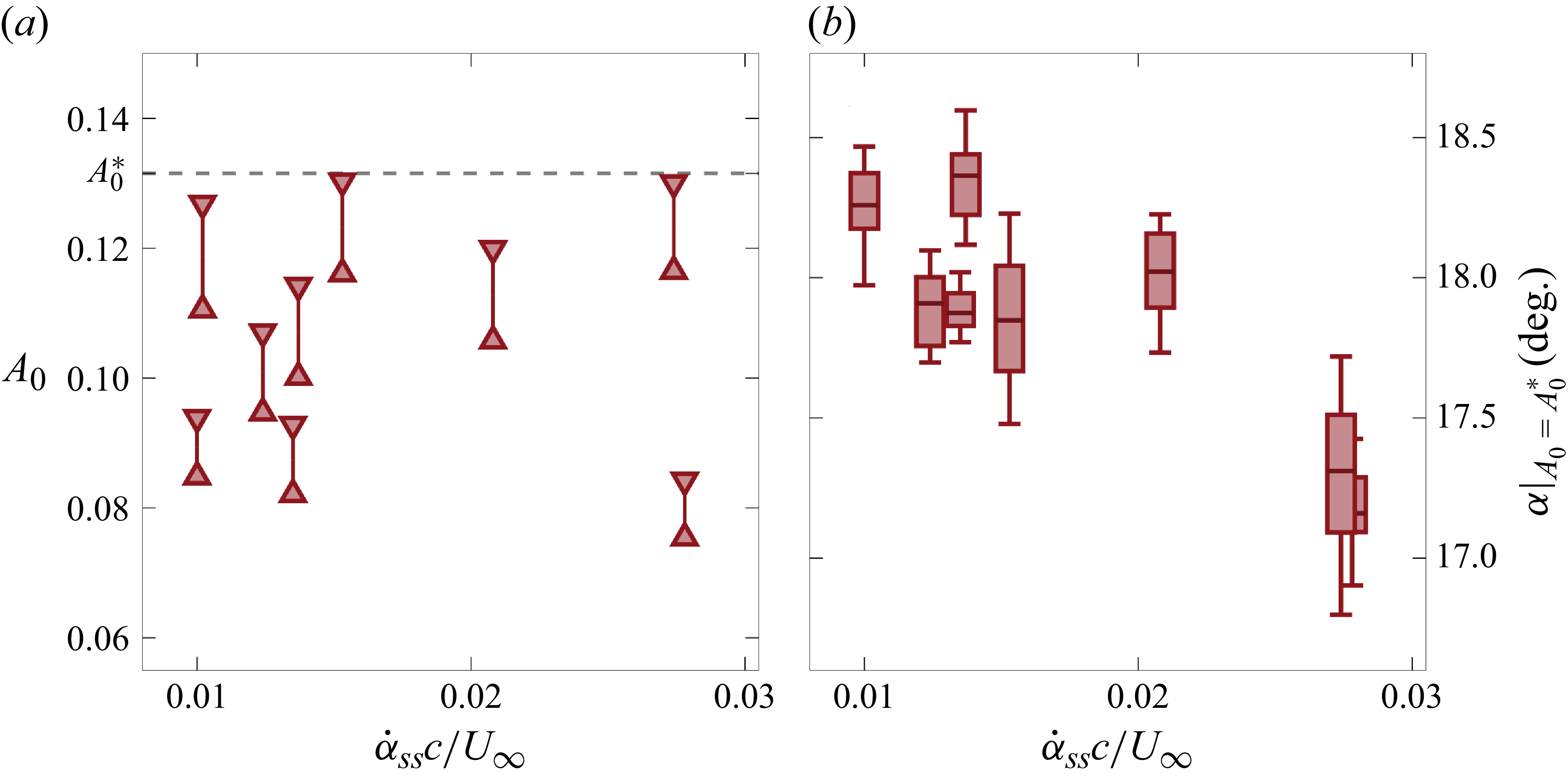


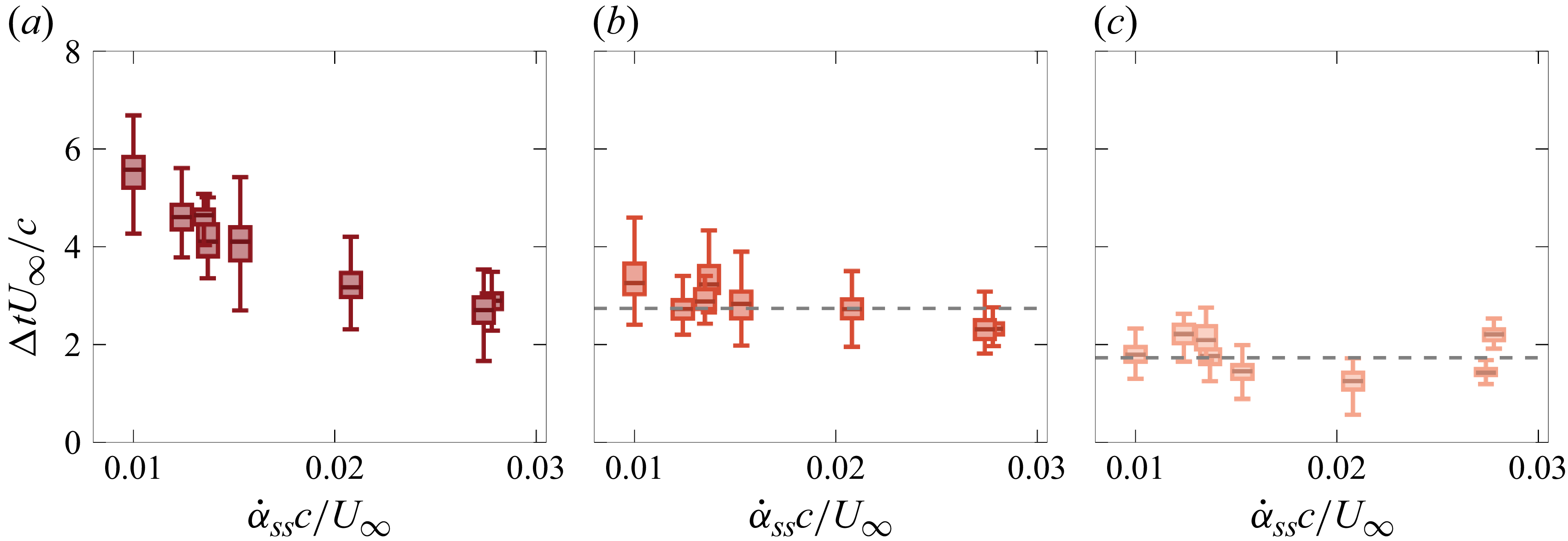


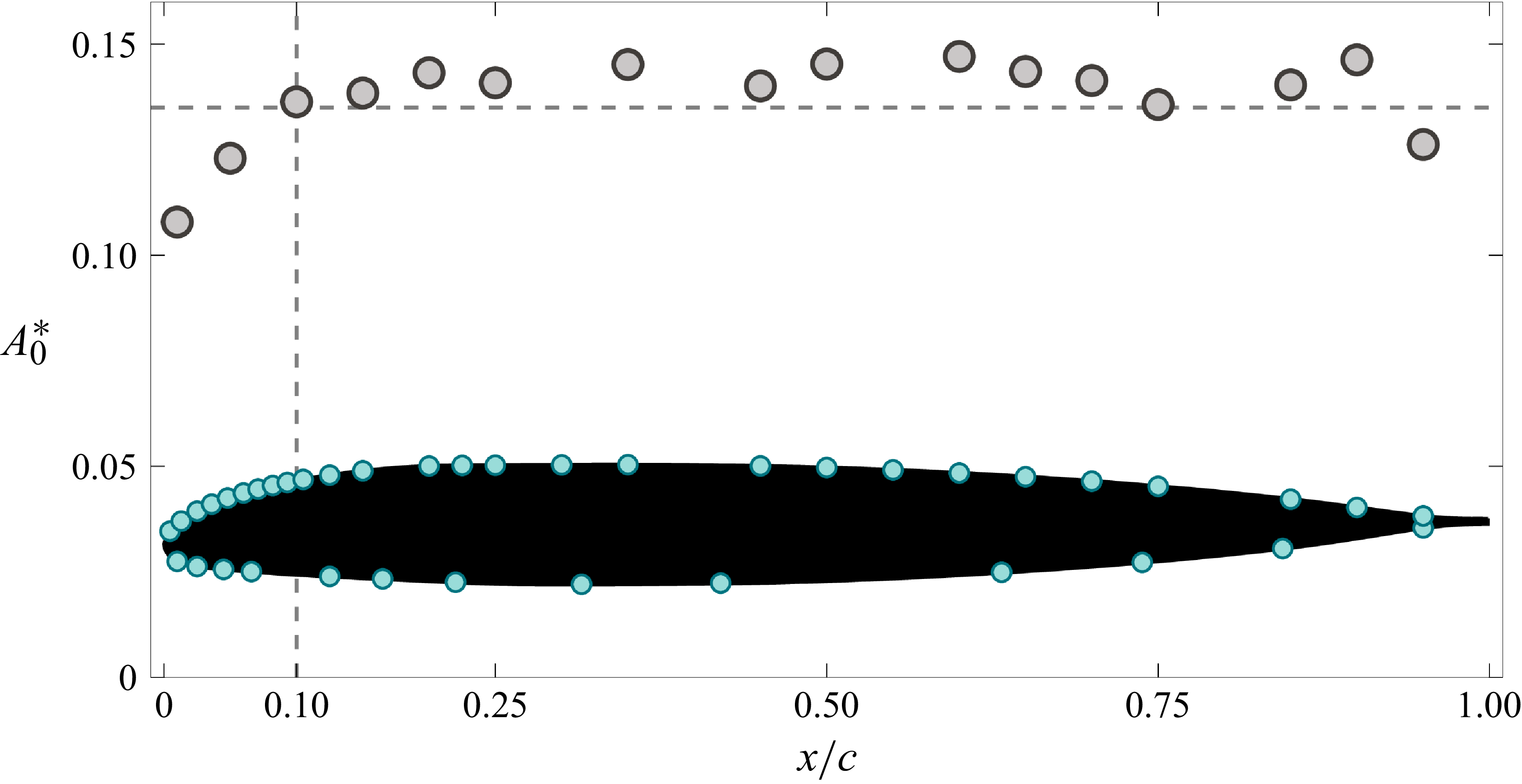


 Open access