


1. Introduction
Flow-induced vibrations (FIV) of bluff bodies placed in a cross-current are ubiquitous in nature, e.g. oscillations of plants in wind or water streams, and are also common in industrial systems. Their impact on the fatigue damage of engineering structures, such as heat exchanger tubes, chimney stacks, spar hulls, cables or mooring lines, as well as their fundamental interest as paradigms of fluid–structure interaction, have motivated a number of research works, as reviewed, for example, by Blevins (Reference Blevins1990) and Païdoussis, Price & de Langre (Reference Païdoussis, Price and de Langre2010).
The system composed of an elastically mounted, rigid circular cylinder, free to translate along a rectilinear path, i.e. with a single degree of freedom, under the effect of a uniform oncoming flow normal to its axis, represents a canonical problem to study a particular form of FIV, called vortex-induced vibrations (VIV). This system has been extensively examined in prior works, where the direction of motion was either normal to the current (Feng Reference Feng1968; Mittal & Tezduyar Reference Mittal and Tezduyar1992; Hover, Techet & Triantafyllou Reference Hover, Techet and Triantafyllou1998; Khalak & Williamson Reference Khalak and Williamson1999; Shiels, Leonard & Roshko Reference Shiels, Leonard and Roshko2001; Klamo, Leonard & Roshko Reference Klamo, Leonard and Roshko2006; Leontini et al. Reference Leontini, Stewart, Thompson and Hourigan2006; Riches & Morton Reference Riches and Morton2018), aligned with the current (Naudascher Reference Naudascher1987; Okajima, Kosugi & Nakamura Reference Okajima, Kosugi and Nakamura2002; Cagney & Balabani Reference Cagney and Balabani2013; Konstantinidis Reference Konstantinidis2014; Gurian, Currier & Modarres-Sadeghi Reference Gurian, Currier and Modarres-Sadeghi2019; Konstantinidis, Dorogi & Baranyi Reference Konstantinidis, Dorogi and Baranyi2021) or at an arbitrary angle (Brika & Laneville Reference Brika and Laneville1995; Bourguet Reference Bourguet2019; Benner & Modarres-Sadeghi Reference Benner and Modarres-Sadeghi2021). In the following, the directions normal and parallel to the current are referred to as the cross-flow and in-line directions, respectively. For such one-degree-of-freedom oscillators, VIV appear over a well-delimited range of values of the reduced velocity,  $U^\star$, defined as the inverse of the oscillator natural frequency, non-dimensionalized by the inflow velocity and the cylinder diameter. Within this range, body motion and flow unsteadiness, associated with vortex formation in the wake, are synchronized. This mechanism of synchronization is referred to as lock-in. The shape of VIV amplitude evolution as a function of $U^\star$, and flow/body frequency ratio ( $1$ or $0.5$) depend on the orientation of the direction of motion. Vortex-induced vibrations reach amplitudes of the order of one body diameter in the cross-flow direction and one or more orders of magnitude lower in the in-line direction. Under lock-in, the vibration frequency can depart from the oscillator natural frequency, while the vortex shedding frequency can deviate from that observed downstream of a stationary cylinder (Strouhal frequency). Such a deviation is often accompanied by a modification of the von Kármán vortex street and a variety of flow patterns may be encountered in the wake of the vibrating body.
The present study also focuses on the vibrations of a one-degree-of-freedom oscillator. It aims at extending the analysis to curved trajectories by considering that the elastically mounted, rigid cylinder is free to translate along a circular arc. The radius of the circular path is introduced as a new parameter of the problem; the rectilinear trajectory corresponds to the particular case where this radius tends to infinity. The objective here is to examine how path curvature may impact the VIV properties previously described for rectilinear displacements, and more generally, to investigate the possible emergence of novel regimes of the flow–body system.
A few recent studies have considered an elastically mounted, rigid circular cylinder, free to rotate about a pivot point, and they have shown that VIV may also develop in this context (Sung et al. Reference Sung, Baek, Hong and Choi2015; Arionfard & Nishi Reference Arionfard and Nishi2017; Malefaki & Konstantinidis Reference Malefaki and Konstantinidis2018, Reference Malefaki and Konstantinidis2020; Arionfard & Mohammadi Reference Arionfard and Mohammadi2021). Such a physical system differs from the present one by the nature of body motion, i.e. rotation versus translation. Yet, a pivoted cylinder oscillates along a circular path and some observations reported in these prior works may also apply to the present system. These previous works examined symmetrical configurations where the pivot point, i.e. circular path centre, and the cylinder at rest are aligned relative to the current, with the pivot point placed either upstream or downstream of the cylinder. These arrangements are referred to as concave and convex configurations in the following. Over the ranges of pivot arm lengths (or, equivalently, circular path radii) and reduced velocities investigated in these studies,  $0.5$ to $8$ cylinder diameters and $U^\star <14$, respectively, VIV globally resemble those reported in the cross-flow, rectilinear motion case: the amplitude of the cylinder angular oscillation exhibits a single-bell-shaped evolution over a range of $U^\star$ where vortex shedding and body motion frequencies coincide. The cross-flow displacement amplitudes reached by the pivoted cylinder are comparable to the rectilinear VIV amplitudes. A specific feature can however be noted. The value of $U^\star$ at which the peak of vibration amplitude occurs tends to increase in the concave configuration, compared with the rectilinear motion case, and to decrease in the convex configuration. This shift is enhanced as arm length is reduced or, equivalently, as path curvature magnitude is increased. It may be connected to the effect of the mean in-line force (also called drag hereafter) exerted by the fluid on the cylinder once it is placed in flow, which tends to increase (reduce, respectively) the stiffness of the oscillator in the concave (convex, respectively) configuration (Malefaki & Konstantinidis Reference Malefaki and Konstantinidis2018).
Prior works concerning the related problem of a tethered cylinder, i.e. a pivoted body without elastic restoring force, immersed in a cross-current, have investigated the vibrations arising in the concave configuration (Ryan Reference Ryan2011; Dominguez, Piedra & Ramos Reference Dominguez, Piedra and Ramos2021). Sharp variations of body response amplitude were reported in the low arm length range, typically below  $0.5$ diameters. Tethered body studies have also analysed the system behaviour when vibrations develop about an asymmetrical position, under the effect of gravity in this case (Carberry & Sheridan Reference Carberry and Sheridan2007; Ryan, Thompson & Hourigan Reference Ryan, Thompson and Hourigan2007). As shown in the following, such asymmetrical arrangements may occur for the present system in the convex configuration, when the equilibrium position shifts due to the mean drag. This aspect was not addressed in the above mentioned works concerning elastically mounted bodies. Angular oscillations about an asymmetrical position are associated with an alteration of the anti-symmetrical organization of the vortex shedding patterns, as well as an asymmetry of fluid forces, with, in particular, the emergence of a mean cross-flow force. It can be noted that comparable symmetry breaking phenomena may exist for rectilinear vibrations in an arbitrary direction (e.g. Bourguet Reference Bourguet2019).
The objective of the present work is to explore the behaviour of the flow–body system when the cylinder is elastically mounted and free to translate along a circular arc. Among other aspects and based on the insights gained from prior pivoted cylinder studies, two elements that need to be investigated are the regimes encountered in the range of low path radii, and the appearance of vibrations after reconfiguration about asymmetrical positions. In order to provide a global vision of the system behaviour, the exploration is carried out over a wide parameter space: for path radii varying from  $0.05$ to $10$ body diameters, in the concave and convex configurations, and for reduced velocity values up to $U^\star =30$. The cross-flow, rectilinear motion configuration is also considered for comparison purposes. As a first step in this work, the Reynolds number based on the cylinder diameter and current velocity is set to $100$. This value ensures that the flow remains two dimensional and, thus, permits precise inspection of the parameter space via two-dimensional numerical simulations.
The paper is organized as follows. The physical system, its modelling and the numerical method are presented in § 2. The system behaviour is examined in § 3, through a joint analysis of the structural response, flow physics and fluid forces. The main findings of this study are summarized in § 4.
2. Formulation and numerical method
The flow–body system and its modelling are described in § 2.1. The numerical method employed and its validation are presented in § 2.2.
2.1. Physical system
The general configuration of the physical system is schematized in figure 1(a). The  $(x,y,z)$ frame is fixed. The elastically mounted, rigid circular cylinder of diameter $D$ and mass per unit length $M_c$ is parallel to the $z$ axis and placed in an incompressible, uniform cross-current of velocity $U$, density $\rho _f$, viscosity $\mu$ and aligned with the $x$ axis. The Reynolds number, $Re=\rho _f U D/\mu$, is set to $100$, which ensures that the flow is two dimensional across the parameter space investigated. This point has been verified via a number of three-dimensional simulations, including when three-dimensional flow fields are used as initial conditions. The two-dimensional Navier–Stokes equations are thus employed to predict the flow dynamics.
Sketch of the physical system: (a) general configuration of the oscillator; the present work focuses on the (b) concave and (c) convex configurations.

The cylinder is free to translate along a circular path of radius  $R$, parallel to the $(x,y)$ plane and centred at the origin of the $(x,y,z)$ frame. The stiffness of the elastic support is denoted by $K$. The cylinder equilibrium position in quiescent fluid is identified by the angle $\theta _0$. The angle $\theta$, referred to as the angular displacement, designates the deviation from this equilibrium position. The cylinder diameter, the current velocity and the fluid density are used to non-dimensionalize the physical variables. In the rest of the paper all the variables are non-dimensional and the term non-dimensional is often omitted to simplify the reading. The non-dimensional, curvilinear displacement of the cylinder along the circular path, about its equilibrium position in quiescent fluid, can be expressed as $\zeta =r\theta$, where $r=R/D$ is the non-dimensional radius of curvature. The in-line, cross-flow and tangential force coefficients are defined as $C_x=2 F_x /\rho _f D U^2$, $C_y=2 F_y /\rho _f D U^2$ and $C=2 F /\rho _f D U^2$, where $F_x$, $F_y$ and $F$ are the dimensional fluid forces per unit length, aligned with the $x$ and $y$ axes, and the direction of body motion, respectively. The tangential force coefficient can be expressed as
 \begin{equation} C={-}C_x \sin\left(\theta+\theta_0\right) + C_y \cos\left(\theta+\theta_0\right). \end{equation}
The dynamics of the one-degree-of-freedom oscillator is governed by the equation
 \begin{equation} \ddot{\zeta} + \left(\dfrac{2{\rm \pi}}{U^\star}\right)^2 \zeta = \dfrac{C}{2m}, \end{equation}
where  $\dot {\phantom {a}}$ designates the non-dimensional time derivative. The mass ratio is defined as $m=M_c/(\rho _f D^2)$ and it is set equal to $10$. The reduced velocity is defined as ${U^\star }=1/f_n$, where $f_n=D/(2{\rm \pi} U)\sqrt {K/M_c}$ is the non-dimensional natural frequency in vacuum. No structural damping is considered to allow maximum amplitude oscillations.
Two symmetrical configurations of the oscillator are examined in this work, the concave ( $\theta _0=0^\circ$) and convex ( $\theta _0=180^\circ$) configurations, which are depicted in figure 1(b,c). To facilitate the presentation of the results, the signed, non-dimensional curvature is introduced: $\kappa =1/r$ in the concave configuration and $\kappa =-1/r$ in the convex configuration. For each configuration (concave or convex), $r$ is varied from $0.05$ to $10$, i.e. $|\kappa |\in [0.1,20]$, and $U^\star$ ranges from $1$ to $30$. This parameter space is substantially wider than those considered in prior studies concerning elastically mounted, pivoted cylinders, especially in the regions of low path radii and large reduced velocities. The cross-flow, rectilinear motion configuration, considered for comparison purposes, is denoted symbolically by $r=\infty$ ( $\kappa =0$). In this configuration $\zeta$ designates the non-dimensional, cross-flow displacement and the forcing term on the right-hand side of the dynamics equation (2.2) is $C_y/(2m)$. As previously mentioned, no structural damping is included. It can however be noted that additional simulations (not presented here) show that the principal features of the system behaviour, in particular the different interaction regimes uncovered in this work, persist when a low level of structural damping is considered.
2.2. Numerical method
The numerical method is the same as in previous studies concerning comparable physical systems, i.e. elastically mounted cylinders in a cross-current at  $Re=100$ (e.g. Bourguet & Lo Jacono Reference Bourguet and Lo Jacono2014; Bourguet Reference Bourguet2019). Descriptions of the simulation approach, boundary conditions and discretizations, as well as detailed validations were reported in these prior works. Only a brief summary of the method and some additional convergence results are presented here.
The coupled flow–body equations are solved by the parallelized code Nektar, which is based on the spectral/ $hp$ element method (Karniadakis & Sherwin Reference Karniadakis and Sherwin1999). Body motion is taken into account by adding inertial terms in the Navier–Stokes equations (Newman & Karniadakis Reference Newman and Karniadakis1997). A large rectangular computational domain is considered ( $350D$ downstream and $250D$ in front, above and below the cylinder) in order to avoid any spurious blockage effects due to domain size. The computational domain is discretized in $3975$ spectral elements. A no-slip condition is applied on the cylinder surface. The free-stream value is assigned for the velocity at the upstream boundary. At the downstream boundary, a Neumann-type boundary condition is used. Flow periodicity conditions are employed on the upper and lower boundaries.
A convergence study in a typical case of large-amplitude vibrations, encountered for low path radii in the convex configuration, is presented in figure 2. The evolutions of the relative difference with respect to the fifth-order simulation results for the curvilinear displacement amplitude, vibration frequency ratio ( $f_\zeta /f_n$, where $f_\zeta$ is the dominant vibration frequency), time-averaged in-line force coefficient and root-mean-square (r.m.s.) value of the tangential force coefficient fluctuation are plotted as functions of the spectral element polynomial order. In this figure and in the following, $\tilde {\phantom {a}}$ designates the fluctuation about the time-averaged value denoted by $\bar {\phantom {a}}$, and the subscript $\phantom {}_{max}$ designates the maximum value. The displacement amplitude is quantified by the maximum fluctuation about the time-averaged value, $\tilde {\zeta }_{max}$. A polynomial order equal to $4$ is selected since an increase from order $4$ to $5$ has no significant impact on the results. It has also been verified that dividing the non-dimensional time step by $2$ (from $0.0025$ to $0.00125$) results in less than $0.1\,\%$ of relative differences on force and displacement statistics.
Relative difference with respect to the fifth-order simulation results as a function of the polynomial order: (a) curvilinear displacement amplitude and vibration frequency ratio, (b) time-averaged in-line force coefficient and r.m.s. value of the tangential force coefficient fluctuation, for  $(r,\kappa,U^\star )=(0.111,-9.001,20)$.

The simulations are initialized with the established periodic flow past a stationary cylinder at  $Re=100$, then the body is released without initial velocity ( $\dot {\zeta }=0$). Prior works concerning VIV have shown that the system may exhibit hysteretic behaviours (e.g. Singh & Mittal Reference Singh and Mittal2005). Additional simulations with different initial conditions (not presented) confirm that hysteresis occurs at the edge of the interaction regimes reported in this paper. The width of the hysteresis loops in terms of $U^\star$ is typically lower than $0.5$ and a detailed investigation of this phenomenon would require a dedicated study, with a refined resolution in specific regions of the parameter space. The present analysis is based on time series of more than $40$ oscillation cycles, collected after convergence of the time-averaged and r.m.s. values of the fluid force coefficients and body displacement.
3. Flow–body system behaviour
In order to illustrate the comportment of the flow–body system across the parameter space investigated, its evolution in five typical cases is depicted in figure 3, via selected time series and spectra of some physical variables. For each case, the cylinder curvilinear displacement fluctuation, the cross-flow component of flow velocity fluctuation ( $\tilde {v}$) sampled $10$ diameters downstream of the body, the tangential force coefficient and the power coefficient defined as $e=C\dot {\zeta }$ are plotted over two cycles of body oscillation, once the permanent state is reached (a,c,e,g,i). The time-averaged curvilinear and angular displacements of the cylinder are indicated above the time series in each case. The corresponding spectra (b,d, f,h,j) are issued from fast Fourier transform over long time series. For each physical variable, the spectral amplitude is normalized by its maximum value and the frequency range is normalized by the dominant vibration frequency. In this figure and in the rest of the paper, the cases considered are designated by the triplet $(r,\kappa,U^\star )$; even if $r$ and $\kappa$ are directly linked ( $r=1/|\kappa |$), this redundancy is adopted to facilitate the localization in the parameter space.
Selected time series (a,c,e,g,i) and associated frequency spectra (b,d, f,h,j) of the cylinder curvilinear displacement fluctuation, cross-flow component of flow velocity fluctuation in the wake, tangential force coefficient and power coefficient, for (a,b)  $(r,\kappa,U^\star )=(0.5,2,6.5)$ (locked 1 : 1 regime), (c,d) $(r,\kappa,U^\star )=(0.062,-16,25)$ (locked 1 : 1 regime), (e, f) $(r,\kappa,U^\star )=(0.175,-5.714,22)$ (locked 2 : 1 regime), (g,h) $(r,\kappa,U^\star )=(0.111,-9.001,20)$ (locked 3 : 1 regime) and (i,j) $(r,\kappa,U^\star )=(0.1,10,20)$ (unlocked regime). The time-averaged curvilinear and angular displacements are indicated above the time series in the left panels. The time series are plotted over two periods of body oscillation. The time intervals over which the flow excites/damps body motion, i.e. positive/negative values of $e$, are denoted by yellow/grey areas. In the right panels the spectral amplitude is normalized by its maximum value for each variable. The frequency range is normalized by the dominant vibration frequency. The natural frequency of the oscillator in vacuum, the modified natural frequency taking into account the drag (3.3) and the vortex shedding frequency in the fixed body case (Strouhal frequency, $St=0.164$) are indicated by green dashed-dotted, grey dashed and blue dotted lines, respectively.
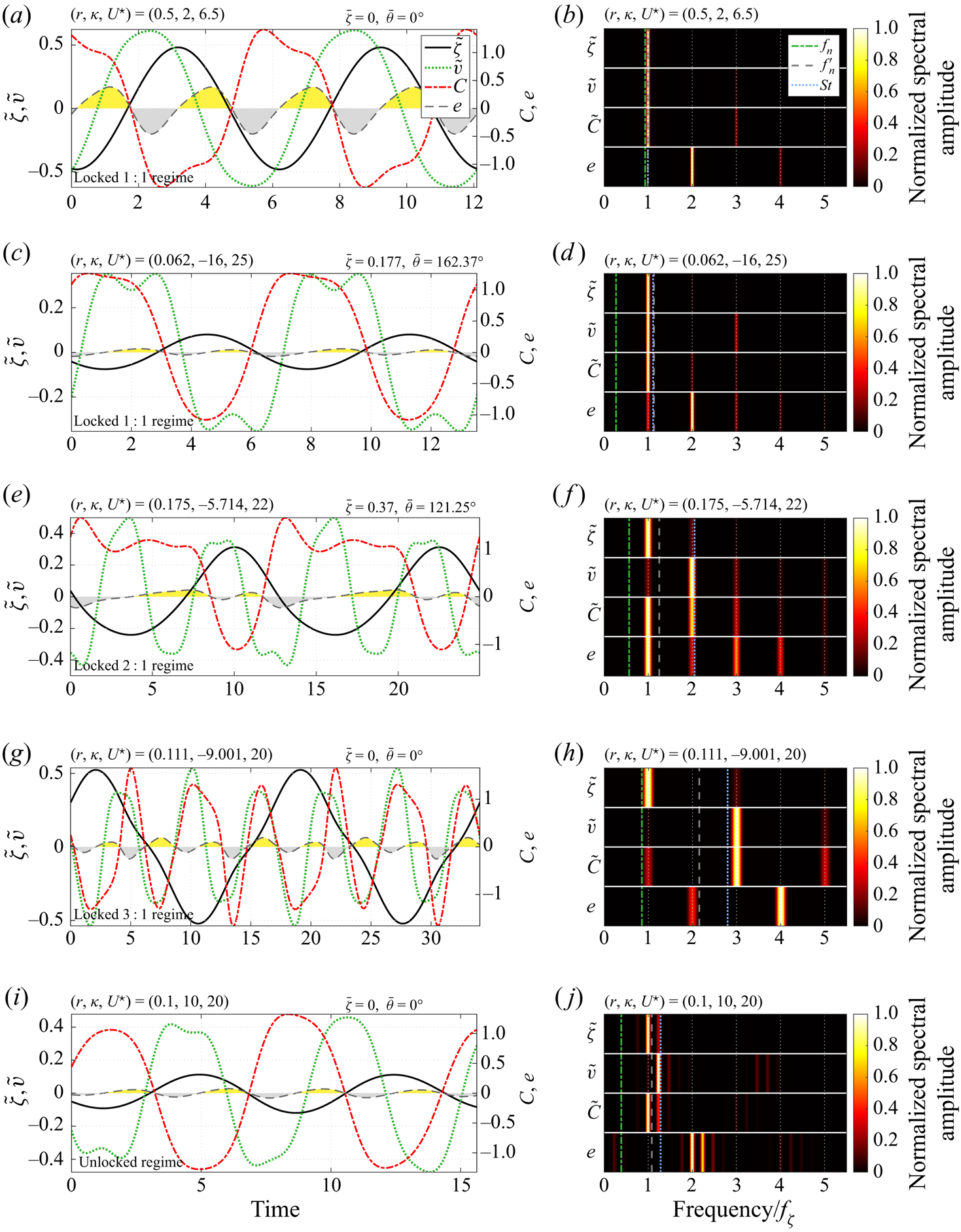
The signals presented in figure 3 cover the different aspects of the system behaviour that will be examined in this work: the structural response (§ 3.1), flow dynamics and its possible synchronization with body motion, which will be used to distinguish the interaction regimes (§ 3.2), and fluid forcing (§ 3.3). Each element of the figure will be described step-by-step in the corresponding subsection. A first overview however reveals contrasted trends among the selected cases, e.g. a variety of amplitudes and frequency contents, diverse symmetry properties and connections between body response and flow fluctuation, different deviations from the natural frequency in vacuum (green dashed-dotted line) and Strouhal frequency (blue dotted line), non-zero time-averaged displacement in some cases, which betrays a reconfiguration of the oscillator. As explained in the following, the cases depicted in figure 3 actually represent the distinct regimes of the system.
3.1. Structural response
The response of the elastically mounted body is explored across the  $(r,U^\star )$ parameter space for the concave and convex configurations depicted in figure 1(b,c). The time-averaged displacement and the possible reconfiguration of the oscillator are examined in § 3.1.1. Then, focus is placed on the amplitude and frequency of vibration, which are studied in §§ 3.1.2 and 3.1.3, respectively.
3.1.1. Time-averaged displacement and reconfiguration
The concave and convex configurations are characterized by a cross-flow symmetry about the  $x$ axis, which suggests that the time-averaged position of the cylinder in flowing fluid should match its equilibrium position in quiescent fluid, i.e. $\bar {\theta }=0^\circ$. A shift from this equilibrium position may however occur, under the effect of mean fluid forcing. Such a shift results in a reconfiguration of the oscillator that breaks the cross-flow symmetry of the system since it introduces an asymmetry in the cylinder trajectory.
The shift due to mean fluid forcing can be estimated a priori, based on the only knowledge of the time-averaged force exerted on a stationary cylinder, by considering a static version of (2.2), i.e.
 \begin{equation} \dfrac{8{\rm \pi}^2 m r}{U^{{\star} 2}} \theta_{eq} ={-} \bar{C}^{f}_x \sin\left(\theta_{eq}+\theta_0\right), \end{equation}
where  $\theta _{eq}$ designates the angular position of the predicted equilibrium and $C^{f}_x$ denotes the in-line force coefficient in the fixed body case ( $\bar {C}^{f}_x=1.32$ at $Re=100$). In the absence of vibration, $\theta _{eq}$ is equal to $\bar {\theta }$; a deviation appears when the body vibrates, as the right-hand side of (3.1) departs from $\bar {C}$. Based on (3.1), no shift is expected in the concave configuration ( $\theta _0=0^\circ$), while a shift is predicted in the convex configuration ( $\theta _0=180^\circ$) when
 \begin{equation} U^\star{>}\sqrt{\dfrac{8{\rm \pi}^2 m r}{\bar{C}^{f}_x}}\approx 24.45 \sqrt{r}. \end{equation}
It is recalled that the mass ratio  $m$ is equal to $10$.
$10$.
The time-averaged position issued from the flow–body system simulation is plotted in figures 4 (concave configuration) and 5 (convex configuration) as a function of the reduced velocity, over a range of path radii (black dots). In these figures panels (a) represent the results obtained in the cross-flow, rectilinear motion configuration. In the other panels, body position is reported in terms of curvilinear (left axis) and angular (right axis) displacements. The equilibrium position predicted via (3.1) is denoted by a black dashed line. In the concave configuration no shift of the time-averaged position is observed relative to the position in quiescent fluid, as indicated by the above static analysis. A shift may occur in the convex configuration. The critical value of  $U^\star$ beyond which the reconfiguration arises and the trend of the time-averaged position with $U^\star$ are globally captured by the static analysis. Yet, deviations appear, for example, close to the boundaries of the orange areas in figure 5(h–j), where irregular evolutions are not predicted. They are associated with the emergence of significant vibrations of the body, as shown in § 3.1.2. The background colours in figures 4 and 5 denote the different regimes of the flow–body system; the colour code will be explicited later in the paper.
Time-averaged, maximum and minimum values of the body curvilinear (left axis) and angular (right axis) displacements in the concave configuration, as functions of the reduced velocity, over a range of path radii. The values of path radius and signed curvature are specified in each panel. For comparison purposes, the displacements observed in the cross-flow, rectilinear motion configuration are reported in panel (a). In each case, the dark grey area depicts the displacement range swept by the body. The equilibrium position predicted by (3.1) is represented by a black dashed line (from panel (b)). Black dotted lines indicate  $\theta =\pm 180^\circ$ (from panel (g)). The background colours denote the different regimes of the flow–body system; the regimes are described in § 3.2 and the colour code is explicited in figure 9.

Same as figure 4 in the convex configuration.

A remarkable feature is that the oscillator may recover a time-averaged position that corresponds to its position in quiescent fluid, beyond the onset of reconfiguration (red areas in figure 5l–o). This phenomenon, called symmetry recovery in the following in reference to the cross-flow symmetry of the system before reconfiguration, is not captured by the above analysis that predicts that reconfiguration should occur. Among the cases selected to illustrate the system behaviour in figure 3, three are expected to be subjected to reconfiguration (based on (3.1)); they are depicted in figure 3(c–h). Reconfiguration is actually observed in the first two cases, where  $\bar {\theta }=162.37^\circ$ and $\bar {\theta }=121.25^\circ$, respectively, while the third one exhibits symmetry recovery, i.e. $\bar {\theta }=0^\circ$ vs $\theta _{eq}=153.6^\circ$.
It can be noted that, for low path radii and large reduced velocities, the time-averaged position of the reconfigured oscillator tends towards  $180^\circ$ and the arrangement is then close to the concave configuration.
3.1.2. Vibration amplitude
The maximum and minimum values of the body curvilinear and angular displacements are reported in figures 4 and 5 (blue and green triangles) for the concave and convex configurations, respectively. As previously mentioned, panels (a) represent the results in the rectilinear motion configuration, in order to better visualize the impact of path curvature. The displacement range swept by the body, i.e.  $[\zeta _{min},\zeta _{max}]$ or $[\theta _{min},\theta _{max}]$, where the subscripts $\phantom {}_{min}$ and $\phantom {}_{max}$ denote the minimum and maximum values, is indicated by a dark grey area. The response amplitude values reported hereafter refer to the maximum fluctuation about the time-averaged value ( $\tilde {\zeta }_{max}$, $\tilde {\theta }_{max}$).
The cylinder is found to vibrate throughout the parameter space investigated, with distinct regions of large-amplitude responses. In the concave configuration (figure 4) the cylinder oscillates about its position in quiescent fluid ( $\bar {\theta }=0^\circ$, no reconfiguration), i.e. along a path that is symmetrical relative to the $x$ axis. The magnitudes of its minimum and maximum displacements are identical, as illustrated by the example depicted in figure 3(a). The typical bell-shaped evolution of the vibration amplitude as a function of $U^\star$, observed in the rectilinear path configuration, is progressively distorted as the radius of curvature is reduced. Several elements can be noted. A comparison of figure 4(a) (rectilinear path) and figure 4(b) ( $r=10$) shows that the introduction of a slight curvature of the trajectory has only an imperceptible influence on the response amplitude. The peak value of curvilinear displacement amplitude reached over the $U^\star$ range decreases with $r$, from $0.56$ diameters for $r=10$ (and the rectilinear path case) to $0.1$ diameters for $r=0.05$. Simultaneously, the peak value of angular displacement amplitude increases, up to $120^\circ \unicode{x2013}130^\circ$ below $r=0.1$. The value of $U^\star$ associated with the onset of the large-amplitude responses and the value associated with the peak amplitude tend to increase as $r$ is reduced, while the bell shape of the response amplitude curve widens. The shift of the peak amplitude along the $U^\star$ range as $r$ is varied was previously reported for pivoted cylinders (Malefaki & Konstantinidis Reference Malefaki and Konstantinidis2018). For low path radii, substantial vibrations are encountered until $U^\star =30$, i.e. the largest value examined here, vs $U^\star =8.5$ in the rectilinear path configuration. A kink can be identified in the evolution of the response amplitude with $U^\star$, at the boundary between the yellow and grey striped areas (figure 4e–j). This phenomenon will be connected to a change of interaction regime.
The bell-shaped amplitude region, typical of the rectilinear motion configuration, where the body vibrates along a symmetrical path about its position in quiescent fluid, is also found to persist in the convex configuration (first yellow areas close to  $U^\star =5$ in figure 5). However, contrary to what was observed in the concave configuration, this region tends to shrink and slightly shift towards lower $U^\star$ values when $r$ is reduced. As in the concave configuration, the peak value of curvilinear displacement amplitude in this region decreases, down to $0.08$ diameters for $r=0.05$, while angular displacements close to $100^\circ$ are reached for low path radii. Two large-amplitude vibration regions emerge for $r<0.2$, in the higher range of $U^\star$ values. A first region, encountered around $r=0.17$, is characterized by oscillations of curvilinear and angular amplitudes close to $0.3$ body diameters and $100^\circ$, respectively. These oscillations develop about a reconfigured position, with $\bar {\theta }\approx 120^\circ$ (orange areas in figure 5h–j). An example of such responses is depicted in figure 3(e). A second region appears below $r=0.13$, where the cylinder exhibits a wide range of vibration amplitudes. In this region the curvilinear amplitude reaches $0.58$ diameters and is thus slightly larger than in the rectilinear path configuration, while the angular amplitude exceeds $280^\circ$. The vibrations may occur about a reconfigured position (second yellow and grey striped areas in figure 5m–r) or about the quiescent-fluid position, after symmetry recovery (red areas in figure 5l–o). The cases presented in figure 3(c,g) illustrate these distinct behaviours. In the absence of reconfiguration, or after symmetry recovery, the magnitudes of the maximum and minimum displacements about the time-averaged position are the same, as previously observed in the concave configuration. When the cross-flow symmetry of the trajectory is broken by the reconfiguration, differences exist, for example, around $U^\star =20$ for $r=0.175$ (figure 5i). As also mentioned for the concave configuration, the jumps in the evolution of the response amplitude are related to switches between interaction regimes, that will be clarified later in the paper.
For low path radii and large reduced velocities, typically below  $r=0.075$ and beyond $U^\star =20$, the reconfiguration tends to transform the convex configuration into a concave arrangement ( $\bar {\theta }\approx 180^\circ$). As a result, the vibration amplitudes are comparable for both configurations in this region.
To summarize the above observations, a global vision of the vibration amplitude across the parameter space is proposed in figure 6, which represents the maximum fluctuation of the curvilinear displacement about its time-averaged value, as a function of the signed curvature and reduced velocity. It is recalled that the signed curvature  $\kappa$ is the inverse of path radius affected with a positive sign in the concave configuration and a negative sign in the convex configuration; $\kappa =0$ designates the rectilinear path configuration, which corresponds to the transition between the concave and convex configurations. All the cases examined in figures 4 and 5 are gathered in figure 6(a). A map, which provides a complementary and more continuous visualization of the vibration amplitude, is plotted in figure 6(b). The cases depicted in figure 3 are indicated by blue points in the map.
Curvilinear displacement amplitude as a function of the signed curvature and reduced velocity: (a) three-dimensional view of the cases depicted in figures 4 and 5, and (b) isocontours. In panel (b) white dashed lines delimit the significant vibration regions ( $\tilde \zeta _{max}\geq 0.05$), which are designated by Roman numerals (I, II, III). The dotted area indicates the region where the oscillator is subjected to reconfiguration, i.e. $\bar {\zeta }\ne 0$. The cases considered in figure 3 are denoted by blue points.

The three regions of the parameter space where the curvilinear displacement amplitude is larger than or equal to  $0.05$ diameters are delineated by white dashed lines in figure 6(b). These regions are identified by Roman numerals (I, II, III) and referred to as the significant vibration regions in the following. The vibration region I extends across the entire range of curvatures investigated. Its evolution with $\kappa$ highlights the distortion of the typical bell-shaped amplitude curve associated with rectilinear vibrations ( $\kappa =0$). The two other significant vibration regions arise in the convex configuration. The area where the oscillator is subjected to reconfiguration, which includes the vibration region II and a portion of region III, is indicated by white dots in the map. The peak-amplitude part of region III represents an island of symmetry recovery in the reconfiguration area.
3.1.3. Vibration frequency
The vibrations are periodic or close to periodic in all studied cases. As illustrated by the examples selected in figure 3, the vibration spectrum is generally dominated by a single frequency, denoted by  $f_\zeta$ and referred to as the vibration frequency. The possible emergence of higher harmonics or incommensurable components is discussed at the end of this subsection.
In figures 7 and 8 the vibration frequency normalized by the natural frequency in vacuum is plotted as a function of the reduced velocity over the range of path radii examined in figures 4 and 5, for the concave and convex configurations. To ease interpretation, different symbols are employed within and outside the significant vibration regions identified in figure 6(b), i.e.  $\tilde {\zeta }_{max}\geq 0.05$ vs $\tilde {\zeta }_{max} < 0.05$. Outside these regions, the vibration frequency (green triangles) is close to the Strouhal frequency ( $St=0.164$, black dotted line), as also noted in previous studies concerning rectilinear oscillations at comparable Re (e.g. Shiels et al. Reference Shiels, Leonard and Roshko2001; Bourguet & Lo Jacono Reference Bourguet and Lo Jacono2014). Within the significant vibration regions, the vibration frequency (blue squares) may substantially depart from St. It remains relatively close to the natural frequency in vacuum for $r>0.2$. Yet, major deviations can be observed for lower path radii, in both configurations, with frequency ratios larger than $4$.
$4$.
Dominant frequencies of body vibration and wake fluctuation in the concave configuration, as functions of the reduced velocity, over a range of path radii. The values of path radius and signed curvature are specified in each panel. For comparison purposes, the frequencies observed in the cross-flow, rectilinear motion configuration are reported in panel (a). The frequencies are normalized by the natural frequency of the oscillator in vacuum. Distinct symbols are used to designate the vibration frequency within and outside the significant vibration regions ( $\tilde {\zeta }_{max}\geq 0.05$ vs $\tilde {\zeta }_{max} < 0.05$). The vortex shedding frequency in the rigidly mounted body case (Strouhal frequency, $St=0.164$) and the modified natural frequency taking into account the mean drag ((3.3), from panel (b)) are indicated by a black dotted line and a black dashed line, respectively. The background colours denote the different regimes of the flow–body system; the regimes are described in § 3.2 and the colour code is explicited in figure 9.

Same as figure 7 in the convex configuration. In panels (h–j) and (l–o), the  $`\times$’ and $`+$’ symbols designate $1/2$ and $1/3$ of the wake fluctuation frequency, respectively.

Prior works concerning pivoted cylinders suggested to take into account the effect of the mean in-line force to modify the expression of the natural frequency of the oscillator in vacuum (Arionfard & Nishi Reference Arionfard and Nishi2017; Malefaki & Konstantinidis Reference Malefaki and Konstantinidis2018). By considering small oscillations about the equilibrium position predicted by the static analysis (3.1), a modified natural frequency can be defined as
 \begin{equation} f'_n=\sqrt{f^2_n+\dfrac{\bar{C}^{f}_x}{8{\rm \pi}^2 m r}\cos(\theta_{eq}+\theta_0)}. \end{equation}
The derivation of  $f'_n$ is explained in an appendix dedicated to a quasi-steady analysis of fluid forcing (Appendix A). Equation (3.3) indicates that the influence of the mean drag on the natural frequency should be more pronounced for low path radii and tends to vanish as the trajectory gets closer to rectilinear. In the absence of reconfiguration ( $\theta _{eq}=0^\circ$), it predicts that the mean force increases the natural frequency in the concave configuration ( $\theta _0=0^\circ$) and reduces it in the convex configuration ( $\theta _0=180^\circ$). Under the assumption that a peak of vibration occurs when the natural frequency $f'_n$ coincides with St, a shift of this peak towards higher (lower, respectively) $U^\star$ values is expected in the concave (convex, respectively) configuration, compared with the rectilinear path configuration. This phenomenon, also reported by Malefaki & Konstantinidis (Reference Malefaki and Konstantinidis2018), is actually observed in region I (figure 6b). After reconfiguration, the effect of the mean drag on the natural frequency depends on the equilibrium position.
In the significant vibration regions,  $f_\zeta$ is found to globally follow the trend of $f'_n$, which is represented by a black dashed line in figures 7 and 8, and by a grey dashed line in the spectra of figure 3. An exception can however be noted in the red areas in figure 8. In this part of the parameter space, the oscillator is subjected to symmetry recovery, which is not captured by the above analysis, and the vibration frequency is found to be close to $f_n$.
Another element can be noted. The vibrations observed in the orange and red areas in figure 8 occur at frequencies relatively close to  $St/2$ and $St/3$, respectively. Such a coincidence suggests that these vibrations could develop under a subharmonic synchronization with the wake, i.e. at a submultiple of wake unsteadiness frequency. This aspect will be clarified in the following.
Some higher harmonic contributions may emerge in the vibration spectrum. Their magnitudes are small in all cases, typically lower than  $15\,\%$ of the fundamental component amplitude, but they reflect the symmetry of the vibration. For periodic responses in the absence of reconfiguration, or after symmetry recovery, only odd harmonics are encountered and the displacement is thus symmetrical about the time-averaged position (figure 3g,h). Once the cross-flow symmetry of the trajectory is altered by the reconfiguration, even harmonics may also appear (figure 3f). In certain regions of the parameter space, incommensurable components of low magnitudes arise in the vibration spectrum (figure 3j). They break the periodicity of the oscillation. They also break its strict cross-flow symmetry, even though the magnitudes of the maximum and minimum displacements measured over a large number of cycles are identical.
The above observations concerning the structural response raise the question of the nature of the interaction between the flow and the vibrating body. This is the object of the next subsection.
3.2. Interaction regimes
This subsection focuses on the connection between the behaviour of the elastically mounted cylinder and flow dynamics. An analysis of the synchronization between body motion and flow unsteadiness leads to the identification of different interaction regimes in § 3.2.1. The spatiotemporal organization of the wake is more specifically examined in § 3.2.2.
3.2.1. Flow–body synchronization – regime identification
For each case depicted in figure 3, flow unsteadiness is represented by a time series of the cross-flow component of flow velocity fluctuation ( $\tilde {v}$), sampled $10$ diameters downstream of the cylinder, at $(x,y)=(10+r\cos (\theta _0),0)$. A comparison of these signals with the time series of body displacement, and the associated spectra, suggest that distinct interaction regimes may develop.
In the parameter space under study, flow unsteadiness, quantified via  $\tilde {v}$ time series, is generally dominated by a single frequency and the contributions of the other spectral components remain marginal. The dominant frequency of flow unsteadiness, denoted by $f_v$ and referred to as flow frequency in the following, is superimposed on the vibration frequency plots in figures 7 and 8 (black dots; the frequencies are normalized by $f_n$ in these plots). Outside the significant vibration regions ( $\tilde {\zeta }_{max} < 0.05$), $f_v$ matches the vibration frequency and is always close to the Strouhal frequency. Once significant structural oscillations occur ( $\tilde {\zeta }_{max} \geq 0.05$), the vibration frequency may substantially deviate from St, as previously noted. However, the condition of synchronization where $f_\zeta =f_v$ is found to persist (yellow areas in the plots). This condition represents the typical lock-in mechanism, usually observed in cross-flow VIV of circular cylinders (Williamson & Govardhan Reference Williamson and Govardhan2004). Examples of such synchronization, in the concave configuration and in the convex configuration in a case where the oscillator is subjected to reconfiguration, are depicted in figures 3(a,b) and 3(c,d), respectively.
Two other forms of flow–body synchronization are uncovered within the significant vibration regions, in the convex configuration. First, the vibration frequency can coincide with  $f_v/2$, which is specified by the ‘ $\times$’ symbols in figure 8h–j) (orange areas). Second, the vibration frequency can be equal to $f_v/3$, indicated by the ‘ $+$’ symbols in figure 8(l–o) (red areas). The deviations of the dominant frequency of the flow from St appear to be smaller than those encountered when $f_\zeta =f_v$. Examples of these two additional forms of synchronization are presented in figures 3(e, f) and 3(g,h), respectively. The time series and spectra show that, in spite of some low-amplitude modulations at $f_\zeta$, flow velocity fluctuation is essentially determined by the dominant component at $f_v$, with distinct frequency ratios, $f_v/f_\zeta =2$ and $f_v/f_\zeta =3$. Flow–body synchronization where the structure oscillates at a submultiple of flow dominant frequency is referred to as subharmonic synchronization hereafter. It is not observed when the circular cylinder is restrained to rectilinear motion, but it was reported in this case for asymmetrical bodies, e.g. a square prism in Zhao et al. (Reference Zhao, Leontini, Lo Jacono and Sheridan2014). Subharmonic synchronization was not detected in previous works concerning elastically mounted, pivoted cylinders; it is recalled that the range of low path radii where such synchronization appears was not explored in these prior studies.
Under flow–body synchronization, regardless of the frequency ratio, the system behaviour is periodic. As previously noted for the structural response, in the absence of reconfiguration, only odd harmonic contributions appear in the flow velocity spectrum. This reflects the strict anti-symmetrical organization of the wake, which will be addressed in § 3.2.2.
In addition to the three forms of flow–body synchronization, a desynchronized state where the body and the flow oscillate at incommensurable frequencies is also encountered in the significant vibration regions, both in the concave and convex configurations (grey striped areas in figures 7d–j and 8m–p). In this desynchronized condition, the vibration frequency follows the modified natural frequency ( $f'_n$), while the dominant frequency of flow unsteadiness is close to St. A typical example is presented in figure 3(i,j). Such a condition resembles the desynchronization or decoherence usually reported for VIV at higher Re, when $U^\star$ is increased beyond the lock-in range (e.g. Khalak & Williamson Reference Khalak and Williamson1999). It should however be mentioned that this condition does not occur at $Re~=100$ when the body moves along a rectilinear path (figure 7a) and its appearance here is thus due to path curvature. Despite their limited amplitudes, the emergence of incommensurable components, at $f_v$ in the vibration spectrum and at $f_\zeta$ in the flow velocity spectrum, results in an aperiodic dynamics of the system, which contrasts with the periodic behaviours encountered under flow–body synchronization.
Based on the different forms of synchronization or desynchronization between the flow and the moving body, determined via the frequencies  $f_v$ and $f_\zeta$, four distinct regimes of interaction can be identified within the parameter space investigated. A first visualization of these regimes is proposed in figure 9, which is used to introduce the nomenclature employed to designate them. This figure represents, for all studied cases, the amplitude of the body curvilinear displacement as a function of the ratio between the flow frequency and vibration frequency. Different symbols are used to distinguish the concave and convex configuration cases. The threshold of the significant vibration regions ( $\tilde {\zeta }_{max}= 0.05$) is specified by a dark grey dashed line. The three regimes where the flow and the body are synchronized with an integer frequency ratio, $f_v/f_\zeta \in \{1,2,3\}$, are referred to as the locked regimes. These regimes are denoted by plain background colours and called locked 1 : 1, locked 2 : 1 and locked 3 : 1, in reference to flow/body frequency ratios. The locked 1 : 1 regime is encountered in the concave and convex configurations, and associated with a wide range of vibration amplitudes, from the lowest amplitudes detected to $0.56$ body diameters. This is the only regime observed outside the significant vibration regions identified in figure 6(b), i.e. $\tilde {\zeta }_{max} < 0.05$, below the dark grey dashed line in figure 9. It is denoted by a yellow background colour, with a lighter tone outside the significant vibration regions. In contrast, the locked 2 : 1 and locked 3 : 1 regimes, which only develop in the convex configuration, are associated with specific ranges of response amplitudes: intermediate amplitudes around $0.3$ diameters in the locked 2 : 1 regime versus large amplitudes close to $0.5$ diameters in the locked 3 : 1 regime, which is the regime where the largest amplitude is measured ( $0.58$). These regimes are indicated by orange and red background colours, respectively. The regime where the flow and the body exhibit incommensurable frequencies, i.e. they are desynchronized, is referred to as the unlocked regime and identified by a grey striped background. It is observed in the concave and convex configurations, and involves vibration of low amplitudes, typically around $0.1$ diameters, and flow/body frequency ratios ranging from $1.1$ to $1.4$.
Curvilinear displacement amplitude as a function of the ratio between the flow frequency and vibration frequency. Distinct symbols are used to designate the concave and convex configuration cases. A dark grey dashed line represents the threshold of the significant vibration regions ( $\tilde {\zeta }_{max}= 0.05$). The integer values of the frequency ratio are specified by black dashed-dotted lines. Plain background colours denote the three regimes where the flow and the body are synchronized, with a frequency ratio of $1$ (locked 1 : 1 regime; yellow/light yellow within/outside the significant vibration regions), $2$ (locked 2 : 1 regime; orange) and $3$ (locked 3 : 1 regime; red). The unlocked regime where the flow and the body are desynchronized is denoted by a grey striped area.

The colour code introduced in figure 9 is used in the backgrounds of figures 4, 5, 7 and 8, to track the different regimes. As in figure 9, a lighter yellow colour is employed to designate the locked 1 : 1 regime out of the significant vibration regions. This continuous monitoring of the interaction regime shows that, within a significant vibration region, the kinks in the evolution of structural response properties, especially vibration amplitude, are generally linked to the passage from one regime to the other. This phenomenon is illustrated by the transition between the locked 1 : 1 and unlocked regimes in figure 4(e–j).
The distribution of the interaction regimes in the  $(\kappa,U^\star )$ parameter space is visualized in figure 10. In this map, the areas associated with the different regimes are delimited by plain black lines and the colour code follows the nomenclature introduced in figure 9. The boundaries of the three regions of significant vibrations identified in figure 6(b) are indicated by dark grey dashed lines. Within these regions, to ease description, the areas associated with distinct regimes are specifically designated (Ia, Ib, IIIa, IIIb and IIIc). The regime names are also mentioned. Two regimes are encountered in region I (locked 1 : 1 and unlocked), a single in region II (locked 2 : 1) and three in region III (locked 1 : 1, locked 3 : 1 and unlocked). This map highlights the pronounced asymmetry of regime distribution relative to the $\kappa =0$ axis, i.e. concave ( $\kappa >0$) versus convex ( $\kappa <0$) configurations. Some symmetry can however be noted for large curvature magnitudes, typically $|\kappa |>13$, beyond $U^\star =20$. As mentioned in § 3.1, the reconfiguration of the oscillator (denoted by black dots in the map) tends to transform the convex configuration into a concave arrangement in this region ( $\bar {\theta }\approx 180^\circ$), which leads to comparable behaviours for $\kappa >0$ and $\kappa <0$. The locked 1 : 1 regime is found to develop over the entire curvature and $U^\star$ ranges investigated. As previously noted, this is the only regime encountered out of the significant vibration regions. The locked 2 : 1 and 3 : 1 regimes appear close to $\kappa =-6$ ( $r\approx 0.17$) and $\kappa =-10$ ( $r\approx 0.1$), for $U^\star \in [17,26]$ and $U^\star \in [15,23]$, respectively. The unlocked regime occurs for $U^\star >9$, and is not observed beyond $|\kappa |\approx 15$ (below $r \approx 0.07$).
Flow–body system regime as a function of the signed curvature and reduced velocity. The areas associated with distinct regimes are separated by plain black lines and the regime names are specified. The colour code used to denote the different regimes is the same as in figure 9. Dark grey dashed lines delimit the significant vibration regions ( $\tilde {\zeta }_{max}\geq 0.05$), which are designated by Roman numerals (I, II, III). The dotted area represents the region where the oscillator is subjected to reconfiguration, i.e. $\bar {\zeta }\ne 0$. The cases considered in figure 3 are indicated by blue points.

The locked 1 : 1 and unlocked regimes arise both in the absence of, or after reconfiguration. This is not the case for the other regimes. The locked 2 : 1 regime is systematically associated with a reconfigured arrangement, while the locked 3 : 1 regime is found to coincide with the island of symmetry recovery detected in the peak-amplitude part of region III (figure 6b). A corollary aspect is that the periodic responses appearing in the locked 3 : 1 regime are strictly symmetrical (odd harmonics only) whereas those developing in the locked 2 : 1 regime are asymmetrical (odd and even harmonics). Both asymmetrical and symmetrical periodic oscillations are encountered in the locked 1 : 1 regime, depending on whether the oscillator is subjected to reconfiguration or not. In the unlocked regime the presence of incommensurable frequency components breaks the oscillation symmetry, regardless of the occurrence of reconfiguration.
The examples selected in figure 3 are localized by blue points in the map. They cover the different regimes observed in the significant vibration regions, including the locked 1 : 1 regime with and without reconfiguration.
The vibrations encountered in the locked 2 : 1 and locked 3 : 1 regimes present similarities with the galloping oscillations observed for non-axisymmetric bodies (Païdoussis et al. Reference Païdoussis, Price and de Langre2010), in particular their relatively large amplitudes, low frequencies compared with flow unsteadiness and the high values of  $U^\star$ where they arise. Some substantial differences can however be noted. The present vibrations develop over finite intervals of $U^\star$ and their amplitudes exhibit bell-shaped evolutions, which contrasts with the typical unbounded growth of galloping oscillation amplitudes. The local occurrence of flow–body synchronization was shown to induce kinks in the evolution of galloping response amplitudes (e.g. Zhao et al. Reference Zhao, Leontini, Lo Jacono and Sheridan2014). Yet, such synchronization is not required for galloping oscillations, since they are driven by a quasi-steady mechanism, decoupled from flow unsteadiness. Here, flow–body synchronization is found to persist, at a subharmonic level, throughout the locked 2 : 1 and locked 3 : 1 regimes and a quasi-steady modelling of fluid forcing fails to predict the present responses, as discussed in Appendix A.
The organization of the wakes associated with the different interaction regimes is investigated hereafter.
3.2.2. Wake organization
In order to shed some additional light on the interaction regimes identified in § 3.2.1, focus is now placed on the flow patterns encountered downstream of the vibrating body. Throughout the parameter space, regardless of the interaction regime, the dominant frequency of flow unsteadiness ( $f_v$) is associated with the formation of a pair of counter-rotating vortices, as in the fixed body configuration. The typical flow patterns observed in the three synchronized regimes, i.e. locked 1 : 1, 2 : 1 and 3 : 1 regimes, are visualized in figures 11, 12 and 13, through instantaneous isocontours of spanwise vorticity. For each selected case, a general view of the wake is presented in the upper panel to show the global structure of the flow and snapshots of the near-wake region, collected every $1/(4 f_v)$ over one period of body oscillation ( $1/f_\zeta$), are plotted in the lower panels, to track vortex formation process. Body trajectory and instantaneous position are indicated in each panel. The vortical pattern formed during one oscillation cycle is enclosed by a dashed grey line in the upper panel and the vortices shed over each half-cycle are separated by a black dashed-dotted line.
Instantaneous isocontours of spanwise vorticity for  $(r,\kappa,U^\star )=(0.5,2,6.5)$ (locked 1 : 1 regime; case considered in figure 3a,b): (a) general visualization of the wake ( $\omega _z\in [-0.5,0.5]$); (b–e) visualization of the near-wake region ( $\omega _z\in [-2,2]$) at four instants over one period of body oscillation, i.e. one period of vortex shedding. The trajectory of the cylinder centre is indicated by a black line. Positive/negative vorticity values are plotted in red/blue. In panel (a) a dashed grey line encloses the vortical pattern formed over one oscillation period and a black dashed-dotted line separates the vortices shed over each half-period. Part of the computational domain is shown.


One pair of alternating vortices is formed per oscillation cycle in the locked 1 : 1 regime, versus two and three pairs in the locked 2 : 1 and 3 : 1 regimes, respectively. In the locked 1 : 1 regime without reconfiguration (figure 11) and in the locked 3 : 1 regime (figure 13), the vortices shed over each half-period of oscillation exhibit anti-symmetrical structures, i.e. a reflection symmetry about the wake centreline, similarly to the von Kármán street observed downstream of a fixed cylinder. The anti-symmetry of wake topology is marked by the absence of even harmonic components in the spectrum of the cross-flow component of flow velocity sampled on the wake centreline, as illustrated in figure 3(b,h). Such organization of the wake coincides with the cross-flow symmetry of cylinder vibrations, i.e. odd harmonics only in the displacement spectrum. The strict anti-symmetry of the locked 1 : 1 regime wakes is perturbed when the body oscillates along an asymmetrical path, due to reconfiguration: slight differences can be noted in the magnitudes and shapes of the positive and negative vortices, even though the overall topology remains close to anti-symmetrical. The six vortices shed over one period of oscillation in the locked 3 : 1 regime tend to regroup into two triplets, which closely resemble the  $2{\rm P}+2{\rm S}$ pattern reported by Williamson & Roshko (Reference Williamson and Roshko1988) under forced rectilinear oscillations near $St/3$. In the locked 2 : 1 regime, two comparable pairs of counter-rotating vortices are formed, one over each half-period of oscillation (figure 12). In contrast to the patterns described above, the vortices shed over each half-period do not present anti-symmetrical structures. In this regime, the body vibrates about a reconfigured position, along an asymmetrical path, and, therefore, no specific symmetry of the wake is expected. It can be noted that the asymmetrical responses (locked 1 : 1 regime with reconfiguration, locked 2 : 1 regime) are not accompanied by major distortion or inclination of the wake, as illustrated by figure 12(a) where the vortices remain globally aligned with the $x$ axis. In the subharmonic synchronization regimes (figures 12 and 13), the rows of the lower panels place side-by-side the two/three successive periods of vortex shedding occurring during one cycle of body oscillation. Even if the vortex formation process is comparable from one shedding period to the other, some subtle differences can be identified, in relation with body motion. For example, in the case depicted in figure 12, the red shear layer developing as the positive vortex is formed appears to be longer in the first period as the body moves upstream (figure 12d,e) than in the second period as it moves downstream (figure 12h,i).
In the unlocked regime, vortex formation and body motion are not synchronized. Based on the flow/body frequency ratio ( $f_v/f_\zeta$), between $2.2$ and $2.8$ vortices are shed per oscillation cycle. The wake resembles that observed downstream of a fixed cylinder, except that its anti-symmetrical organization is slightly altered, as expected in the presence of incommensurable vibrations of the body.
The description of the spatial organization of the wake shows that the typical patterns associated with the different interaction regimes are essentially variations about the von Kármán street occurring in the fixed body configuration. In particular, as previously mentioned, the dominant frequency  $f_v$ always coincides with the shedding of a pair of counter-rotating vortices. Figures 7 and 8 indicate that the shedding frequency can clearly depart from the Strouhal frequency once the body is subjected to significant vibrations and that the magnitude of this departure depends on the interaction regime. To further examine this aspect, the amplitude of the body curvilinear displacement is plotted in figure 14 as a function of the relative deviation of $f_v$ from St, for all studied cases. Distinct symbols are used to distinguish the four interaction regimes and the colour code employed is the same as in figure 9. The limit of the significant vibration regions is denoted by a dark grey dashed line. In the locked 1 : 1 regime, the relative deviation of the shedding frequency is found to vary from $-25\,\%$ to $+20\,\%$, approximately. A pronounced departure from St can be observed both in the concave and convex configurations. A monitoring of the deviation versus path curvature shows that the largest differences are encountered for $|\kappa |<10$ ( $r>0.1$). The frequency range tends to widen as the vibration amplitude increases, up to $0.2$ diameters. It follows a global V shape that roughly matches the boundaries of the wake synchronization region identified by Koopmann (Reference Koopmann1967) for forced rectilinear oscillations, at the same Re (green dotted lines). On the other hand, the locked 2 : 1 and 3 : 1 regimes are associated with specific, narrow ranges of vortex shedding frequencies, slightly lower than St, typically $-2\,\%$, and larger than St, around $+7\,\%$, in the former and latter regimes, respectively. In the unlocked regime the shedding frequency is also restrained to a limited range, with a typical deviation of $-4\,\%$ relative to St. Prior studies concerning forced oscillations have reported comparable deviations towards values lower than St in the absence of synchronization (e.g. Cheng & Moretti Reference Cheng and Moretti1991). This phenomenon could be attributed to the larger apparent diameter of the body seen by the flow, when the cylinder vibrates. A scaling by the effective transverse length covered by the body, instead of $D$, results indeed in a reduction of the frequency but the values are lower than those actually measured, for example, close to $0.85$ St ( $-15\,\%$) in the case depicted in figure 3(i,j).
Curvilinear displacement amplitude as a function of the relative deviation of the flow frequency from the Strouhal frequency. A dark grey dashed line represents the threshold of the significant vibration regions ( $\tilde {\zeta }_{max}= 0.05$). A black dashed-dotted line denotes the absence of deviation ( $f_v=St$). Distinct symbols are employed to designate the interaction regimes, with the colour code introduced in figure 9. Green dotted lines delimit the region of synchronization reported by Koopmann (Reference Koopmann1967) under forced, cross-flow oscillations.

The system exhibits four distinct regimes characterized by different forms of synchronized or unsynchronized interaction between the flow and the vibrating cylinder. Each regime has been associated with typical properties of the structural response and wake organization. Another facet of the interaction relates to fluid forcing, which is addressed in the next subsection.
3.3. Fluid forcing
The description of the system behaviour establishes a close connection between the emergence of vibrations and flow unsteadiness. A quasi-steady analysis of fluid forcing where the effect of flow unsteadiness is neglected is presented in Appendix A. As expected based on the above observations, this approach fails to predict body responses. Some insights can however be obtained from this analysis, concerning, for instance, the modification of the oscillator natural frequency, as discussed in the appendix.
Two elements of fluid forcing are examined in this subsection: the time-averaged in-line force and its amplification once the body vibrates in § 3.3.1, and then, the tangential force, its phasing with body motion and the associated energy transfer in § 3.3.2.
Some additional observations concerning the contributions of the in-line and cross-flow forces to the tangential force are reported in Appendix B. Another complementary aspect, which was documented in tethered body studies (Ryan et al. Reference Ryan, Thompson and Hourigan2007), concerns the appearance of a time-averaged component of the cross-flow force, when the cylinder oscillates along an asymmetrical path. Both positive and negative values of  $\bar {C}_y$ are measured across the reconfiguration area, with mainly negative values in the significant vibration regions, down to a minimum close to $-0.04$. The magnitude of $\bar {C}_y$ remains limited compared with $\bar {C}_x$. This aspect will not be further investigated here.
3.3.1. Time-averaged in-line force
The time-averaged value of  $C_x$ across the $(\kappa,U^\star )$ parameter space is represented in figure 15(a). The range of $\bar {C}_x$ values is indicated on the right axis of the colourbar and the corresponding range of relative deviations from the fixed body case value ( $\bar {C}^{f}_x=1.32$) is specified on the left axis. The limits of the significant vibration regions and distinct regime areas are denoted by white dashed and plain lines, respectively. The different zones of the parameter space are identified as in figure 10. The cases considered in figure 3 are localized by blue points.
(a) Time-averaged value of the in-line force coefficient as a function of the signed curvature and reduced velocity. The range of  $\bar {C}_x$ values is indicated on the right axis of the colourbar and the associated range of relative deviations from the fixed body case value is specified on the left axis. White dashed lines delimit the significant vibration regions and the areas associated with distinct regimes are separated by plain white lines; the area names are those introduced in figure 10. The cases considered in figure 3 are identified by blue points. (b) Relative deviation of the time-averaged value of the in-line force coefficient as a function of the curvilinear displacement amplitude. A dark grey dashed line represents the threshold of the significant vibration regions. Distinct symbols are employed to designate the interaction regimes, with the same colour code as in figure 9. The areas of the significant vibration regions associated with each regime are indicated in the legend. Open blue symbols, with the same shapes as those reported in the legend, represent the results issued from quasi-steady modelling ((A2) in Appendix A).

The time-averaged drag exhibits a peak in region Ia, where the locked 1 : 1 regime is established. The peak appears in the area of large path radii, with a shift towards positive curvatures (concave configurations). In this region,  $\bar {C}_x$ is amplified by $55\,\%$ compared with the fixed body case value. The location of the peak closely coincides with the peak of vibration amplitude depicted in figure 6(b). Such a coincidence was often emphasized in previous works (e.g. Khalak & Williamson Reference Khalak and Williamson1999). To visualize this connection, the deviation from the fixed body case value is plotted as a function of the curvilinear displacement amplitude in figure 15(b). The significant vibration region limit is indicated by a dark grey dashed line and distinct symbols are employed to designate the different regimes (same colour code as in figure 9). The time-averaged in-line force is also enhanced in the locked 2 : 1 and 3 : 1 regimes (regions II and IIIc), even though to a lesser extent, typically around $+6\,\%$ and $+10\,\%$, respectively. It can be noted that the amplification is much less pronounced in the locked 3 : 1 regime than in the locked 1 : 1 regime (region Ia), whereas the response amplitudes are comparable and even larger in the former regime. In spite of the dispersion observed between the different regimes, it appears that for a given locked regime, $\bar {C}_x$ tends to globally increase with vibration amplitude. A slight reduction, down to $-5\,\%$, is however encountered in some regions of low to moderate vibration amplitudes in the locked 1 : 1 regime. A minor reduction of $\bar {C}_x$ is also noted in the unlocked regime.
The above observations indicate that  $\bar {C}_x$ alteration is not strictly determined by the response amplitude. It should be mentioned that the dispersion persists if the cross-flow projection of the displacement is considered, instead of $\zeta$. Prior studies have shown that the response frequency may also play a role (e.g. Carberry, Sheridan & Rockwell Reference Carberry, Sheridan and Rockwell2005). Here, a slightly better collapse of $\bar {C}_x$ can be achieved by considering the product of the response amplitude and frequency, i.e. a typical velocity of the moving cylinder, or the time-averaged relative velocity seen by the body.
For comparison purposes, the time-averaged values issued from the quasi-steady modelling of  $C_x$ ((A2) in Appendix A), based on the structural responses obtained via the unsteady simulation approach, are plotted in figure 15(b) (open blue symbols). The quasi-steady modelling predicts an increase of $\bar {C}_x$ with vibration magnitude, with lower amplifications in the locked 2 : 1 and 3 : 1 regimes than in the locked 1 : 1 regime, as also noted in the unsteady simulation results. The enhancement of the time-averaged force is however not captured, as the maximum amplification only reaches $+10\,\%$ compared with the fixed body case value.
3.3.2. Tangential force, phasing with displacement and energy transfer
The reconfiguration of the oscillator in the locked 1 : 1, locked 2 : 1 and unlocked regimes is accompanied by the emergence of a time-averaged component of the tangential force, which vanishes otherwise. In the locked regimes the tangential force is periodic and synchronized with body motion/flow unsteadiness. Several components may arise in its spectrum but they are all harmonics of the vibration frequency  $f_\zeta$, which represents the fundamental component. Only odd harmonics are encountered when the cylinder vibrates along a symmetrical path. In particular, the projection of the in-line force, which is composed of even harmonics, on the tangential direction (2.1), results in odd harmonics only. Both odd and even harmonics appear once path symmetry is broken by the reconfiguration. The higher harmonic contributions represent a moderate fraction of the first harmonic magnitude in the locked 1 : 1 regime, typically around $20\,\%$, except near the force–displacement phase difference jump where the first harmonic vanishes and the relative magnitude of the higher harmonics is consequently very large; this point will be discussed later in this subsection. They represent a significant fraction of the first harmonic magnitude in the locked 2 : 1 regime, around $70\,\%$, and are even larger in the locked 3 : 1 regime, from $2$ to $10$ times the first harmonic magnitude. In the unlocked regime both vibration and flow frequency components, which are incommensurable, appear in the spectrum of the aperiodic tangential force, as well as their higher harmonics. The higher harmonic contributions are small in this regime, typically lower than $5\,\%$ of the fundamental component magnitudes. These different elements are visualized in figure 3, where the time series of $C$ and corresponding spectra are plotted for each selected case.
The statistics of the tangential force are further examined in figure 16. The r.m.s. value of  $C$ fluctuation and its relative deviation from the r.m.s. value of $C_y$ fluctuation in the fixed body case ( $(\tilde {C}^{f}_y)_{rms}=0.23$) are represented over the parameter space in figure 16(a). The cross-flow force coefficient is chosen as reference since $C=\pm C_y$ in the absence of vibration and reconfiguration. A major amplification of the tangential force fluctuation is observed in all the significant vibration regions (delimited by white dashed lines), not only in the locked regimes but also in the unlocked regime (regions Ib and IIIb). Peak values are encountered in region Ia (locked 1 : 1 regime), where the fluctuation may become six times larger than in the fixed body case. They occur for convex configurations and do not coincide with the peak of the time-averaged drag identified in figure 15(a). A complementary visualization is proposed in figure 16(b) where the deviation from the fixed body case value is plotted as a function of the vibration frequency, normalized by the natural frequency of the oscillator in vacuum. This plot depicts more precisely the typical ranges of force fluctuations associated with the different regimes: a wide dispersion in the locked 1 : 1 and unlocked regimes where the deviation ranges from $-100\,\%$ to $650\,\%$ and from $0\,\%$ to $250\,\%$, respectively, a narrower dispersion in the locked 2 : 1 regime, from $150\,\%$ to $300\,\%$, and a concentration around $300\,\%$ in the locked 3 : 1 regime.
(a) Same as figure 15(a) for the r.m.s. value of the tangential force coefficient fluctuation and its relative deviation from the r.m.s. value of  $C_y$ fluctuation in the fixed body case. The values of the force–displacement phase difference ( $\varphi =0^\circ$ or $\varphi =180^\circ$) are specified in grey and grey dotted lines denote the phase difference jumps. (b) Relative deviation of the r.m.s. value of the tangential force coefficient fluctuation as a function of the vibration frequency normalized by the natural frequency in vacuum. A grey dashed-dotted line denotes the frequency ratio of $1$. The values of the force–displacement phase difference are indicated on each side of this line. Distinct symbols are employed to designate the interaction regimes, with the same colour code as in figure 9. The areas of the significant vibration regions associated with each regime are mentioned in the legend. A light green area delimited by green dotted lines depicts the drop of force fluctuation amplitude occurring close to the phase difference jump in the locked 1 : 1 regime. Open red triangular symbols represent the contribution of the first harmonic of the force (i.e. at $f_\zeta$) in the locked 3 : 1 regime. Part of the parameter space is shown to ease visualization of the phase difference jump region.

Figure 16(b) shows that the vibration frequency crosses the natural frequency of the oscillator in vacuum in the locked 1 : 1 and locked 3 : 1 regimes, while it remains larger than  $f_n$ in the locked 2 : 1 and unlocked regimes. The frequency ratio $f_\zeta /f_n$ is closely linked to the phasing between force and displacement, and to the relative contributions of the different harmonics in the force spectrum (e.g. Gsell, Bourguet & Braza Reference Gsell, Bourguet and Braza2016). The phase difference between the components of $C$ and $\zeta$ occurring at the dominant vibration frequency $f_\zeta$ is denoted by $\varphi$. For periodic responses in the absence of structural damping, the system may exhibit two possible states where the force is either in phase with the displacement ( $\varphi =0^\circ$), when $f_\zeta < f_n$, or in phase opposition ( $\varphi =180^\circ$), when $f_\zeta >f_n$. The phase difference jump occurring during the transition between these two states is accompanied by the disappearance of the force component at vibration frequency. Such a binary behaviour is verified in the three locked regimes, which are periodic: both phasing states are encountered in the locked 1 : 1 and locked 3 : 1 regimes, and $\varphi =180^\circ$ in the locked 2 : 1 regime. In the aperiodic, unlocked regime the phase difference is always equal to $180^\circ$, as illustrated in figure 3(i).
The locations of the force–displacement phase difference jumps as well as the values of the phase difference are indicated in the map of figure 16(a). A jump crosses the area of the parameter space associated with the locked 1 : 1 regime and another delineates a small portion of region IIIc, associated with the locked 3 : 1 regime, where force and displacement are in phase. In figure 16(a) a drop in the magnitude of the tangential force fluctuation can be noted near the phase difference jump in the locked 1 : 1 regime, especially in region Ia close to  $\kappa =0$. In contrast, no drop appears in region IIIc, in the locked 3 : 1 regime. These distinct behaviours are visualized in figure 16(b), where the frequency ratio of $1$, which coincides with the phase difference jumps, is denoted by a grey dashed-dotted line; the values of $\varphi$ are specified on each side of this line. The contrasted trends noted in the locked 1 : 1 and locked 3 : 1 regimes are connected to the relative contributions of the higher harmonics in force fluctuation. In the locked 1 : 1 regime, even if higher harmonics exist in the force spectrum, their magnitudes remain small and the first harmonic (fundamental component at $f_\zeta$) generally dominates. Therefore, when the first harmonic contribution decreases near the phase difference jump, the magnitude of force fluctuation also drops. This drop is depicted by the light green area in figure 16(b). In the locked 3 : 1 regime the contributions of the higher harmonics dominate. This is emphasized in figure 16(b), where the contribution of the first harmonic is indicated by open red triangular symbols. The first harmonic contribution indeed vanishes near $f_\zeta =f_n$, but its evolution has only a negligible impact on the force fluctuation magnitude, which does not substantially change during the jump of the force–displacement phase difference.
The energy transfer between the flow and the moving cylinder is quantified by the power coefficient  $e=C\dot {\zeta }$, as previously defined. The time series and spectra of $e$ in figure 3 illustrate the typical evolutions observed in the different interaction regimes. In the time series the intervals over which the flow excites/damps body motion, i.e. positive/negative values of $e$, are denoted by yellow/grey areas. For regular vibrations, as those reported here and in the absence of structural damping, the time-averaged power coefficient vanishes. More precisely, the power coefficient averaged over one oscillation cycle is equal to zero in the locked regimes (periodic responses). Zero averaged energy transfer is only reached over a number of oscillation cycles in the unlocked regime (aperiodic responses). As expected from its definition, the spectrum of $e$ is composed of even harmonics of the fundamental vibration component ( $f_\zeta$) in the locked regimes without reconfiguration, essentially the second and fourth harmonics in the present cases (figure 3b,h). Odd and even harmonics participate in the energy transfer after reconfiguration (figure 3d, f). In the unlocked regime the spectral components occur at $2f_\zeta$, $2f_v$, $f_v \pm f_\zeta$, and other linear combinations of the fundamental components of body response and flow unsteadiness (figure 3j). Once the permanent behaviour of the system is reached, except for large radii close to the rectilinear path configuration, the energy transfer is dominated by the contribution of the time-averaged in-line force, $\bar {C}_x \dot \zeta _x$, where $\dot \zeta _x=-\dot \zeta \sin (\theta +\theta _0)$ is the in-line projection of body velocity (the contributions of the in-line and cross-flow forces to the tangential force are discussed in Appendix B). This explains why body excitation tends to occur at a comparable phase of the oscillation cycle, i.e. when the body moves downstream, regardless of the interaction regime at play.
This subsection has shed some light on the general properties of fluid forces and emphasized specific features associated with each regime, concerning their amplification, frequency content and phasing. The principal findings of this work are summarized in the next section.
4. Conclusion
The vibrations of an elastically mounted circular cylinder, free to move along a circular arc under the effect of a cross-current, have been examined at  $Re=100$ on the basis of numerical simulation results. The impact of trajectory curvature on the flow–body system behaviour has been explored over a wide parameter space, by considering, for the concave and convex configurations, path radii ranging from $0.05$ to $10$ body diameters and reduced velocity values up to $30$.
$30$.
The cylinder is found to vibrate across the entire parameter space investigated. Path curvature results in a major alteration of the VIV observed for rectilinear displacements and in the emergence of novel interaction regimes. Substantially different evolutions are noted in the concave and convex configurations. Rectilinear VIV are driven by a synchronization mechanism where the frequency of body motion coincides with the frequency of flow unsteadiness associated with vortex shedding. In spite of the distortion of the structural response shape, this lock-in mechanism persists over a range of  $U^\star$ values, for all path radii in both configurations. In addition to this harmonic mechanism, two subharmonic forms of synchronization, at half and one third of flow unsteadiness frequency, are uncovered in the convex configuration, in the range of low path radii. The three synchronized regimes, named locked 1 : 1, 2 : 1 and 3 : 1 regimes in reference to the flow/body frequency ratio, coexist with a desynchronized regime where the body and the flow oscillate at incommensurable frequencies. This regime, called the unlocked regime, appears in the higher- $U^\star$ range in both configurations.
The main characteristics of the four interaction regimes are gathered in table 1 and some salient elements are summarized in the following. The three locked regimes exhibit contrasted properties but they share a common feature that is the periodic nature of the system behaviour, as opposed to the aperiodic dynamics observed in the unlocked regime. In the convex configuration, due to mean fluid forcing, the oscillator may be subjected to a reconfiguration (abbreviated as reconf. in the table), i.e. a shift of the time-averaged displacement from the equilibrium position in quiescent fluid. A reconfiguration breaks the cross-flow symmetry of the system since it introduces an asymmetry in cylinder trajectory. It is thus closely connected to the different symmetry properties of the system behaviour. The locked 1 : 1 and unlocked regimes develop both with or without reconfiguration, while the locked 2 : 1 regime always arises for a reconfigured arrangement. The locked 3 : 1 regime occurs in the reconfiguration region of the parameter space but the oscillator is found to recover its quiescent-fluid position, a phenomenon referred to as symmetry recovery (symmetry recov. in the table).
A wide range of vibration amplitudes is encountered in the locked 1 : 1 regime. The other regimes are associated with more specific amplitude ranges. The largest amplitudes of curvilinear displacement, with a peak value of  $0.58$ body diameters, are measured in the locked 3 : 1 regime. The vibration frequency crosses the natural frequency of the oscillator in vacuum in the locked 1 : 1 and locked 3 : 1 regimes, which corresponds to a jump in force–displacement phase difference. The vibration frequency remains larger than $f_n$ in the locked 2 : 1 and unlocked regimes. After reconfiguration, the structural response presents an asymmetry that is reflected by the emergence of even harmonic components in vibration spectra, as typically observed in the locked 2 : 1 regime.
The flow patterns reported in the different interaction regimes are essentially variations about the von Kármán street occurring in the fixed body configuration, with, in the locked regimes, an integer number of alternating vortex pairs formed per oscillation cycle. The anti-symmetrical organization of the wake is however perturbed when the body vibrates about a reconfigured position and in the unlocked regime. The different regimes are characterized by distinct deviations from the Strouhal frequency. They also exhibit contrasted trends in terms of fluid forcing, in particular concerning force amplification, illustrated by mean drag alteration in table 1, and regarding the contributions of the higher harmonic components, which are found to become prominent in the subharmonic synchronization regimes.
Principal properties of the different regimes identified in this work.

Acknowledgements
This work was performed using HPC resources from CALMIP (grants 2021-P1248 and 2022-P1248).
Funding
This research received no specific grant from any funding agency, commercial or not-for-profit sectors.
Declaration of interests
The author reports no conflict of interest.
Appendix A. Quasi-steady modelling of fluid forcing
Assuming a decoupling of the flow and moving cylinder time scales, a quasi-steady model of the tangential force can be obtained by considering the projection of the time-averaged force aligned with the relative velocity seen by the body. This time-averaged force can be expressed as the time-averaged in-line force coefficient in the fixed body case ( $\bar {C}^{f}_x$), modulated by the squared magnitude of the relative velocity. The components of the relative velocity, normal and tangential to the trajectory of the cylinder located at an angle $\theta$ with a velocity $\dot \zeta$, are equal to $V_n=\cos (\theta +\theta _0)$ and $V_t=\dot \zeta +\sin (\theta +\theta _0)$, respectively. The angle $\beta$ between the relative velocity and the tangential direction satisfies $\tan (\beta )=V_n/V_t$. A quasi-steady model of $C$, identified by the superscript $\phantom {}^{qs}$, can be expressed as
 \begin{align} C^{qs} & ={-}\bar{C}^{f}_x (V^2_n+V^2_t)\cos\left(\beta\right) \end{align}
 \begin{align} & ={-}\bar{C}^{f}_x \left(\dot\zeta+\sin\left(\theta+\theta_0\right)\right)\sqrt{\dot\zeta^2+2\dot\zeta\sin\left(\theta+\theta_0\right)+1}. \end{align}
The value of  $\bar {C}^{f}_x$ depends on the Reynolds number associated with the relative velocity magnitude, which ranges from $73$ to $133$ across the parameter space, based on the unsteady simulation results. Over this range, $\bar {C}^{f}_x$ exhibits a slightly decreasing trend, from $1.35$ to $1.31$, which is taken into account in the subsequent analysis. The quasi-steady model of $C$ is expressed in terms of the angular displacement and curvilinear velocity, i.e. $\theta$ and $\dot \zeta$, as path radius ( $r$) vanishes in this formulation and the different cases can thus be visualized on a single map. The evolution of $C^{qs}$ as a function of $\theta +\theta _0$ and $\dot \zeta$ is represented in figure 17(a). A comparison of $C^{qs}$ and $C$ is proposed in figure 17(b), where the force coefficients are plotted as functions of $\theta +\theta _0$ for three selected cases, representative of the three locked regimes. The value of $C^{qs}$ is based on (A1b) where $\theta$ and $\dot \zeta$, depicted in figure 17(a) for each selected case, are issued from the unsteady simulations. Some significant deviations can be noted but it appears that the global trends of $C$ are roughly captured by the quasi-steady model.
(a) Quasi-steady modelling of the tangential force coefficient (A1b) as a function of the angular position and curvilinear velocity of the body. Plain lines represent the evolutions of the position and velocity issued from the unsteady simulations for three selected cases,  $(r,\kappa,U^\star )=(0.5,2,6.5)$ (locked 1 : 1 regime), $(r,\kappa,U^\star )=(0.175,-5.714,22)$ (locked 2 : 1 regime) and $(r,\kappa,U^\star )=(0.111,-9.001,20)$ (locked 3 : 1 regime). (b) Tangential force coefficients issued from the unsteady simulations (dotted lines) and quasi-steady modelling (plain lines), as functions of the angular position, for the three selected cases depicted in panel (a).

A comparable quasi-steady model can be derived for the in-line force coefficient, i.e.
 \begin{equation} C^{qs}_x = \bar{C}^{f}_x \left(\dot\zeta\sin\left(\theta+\theta_0\right)+1\right)\sqrt{\dot\zeta^2+2\dot\zeta\sin\left(\theta+\theta_0\right)+1}. \end{equation}
The time-averaged values of  $C^{qs}_x$, where $\theta$ and $\dot \zeta$ are issued from the unsteady simulations, are compared with $\bar {C}_x$ in figure 15(b), for all studied cases (open blue symbols). The quasi-steady approach predicts that the time-averaged in-line force increases once the body vibrates, yet the magnitude of force amplification is not captured.
To further assess the validity of the quasi-steady modelling, additional simulations where the force coefficient  $C$ on the right-hand side of the dynamics equation ((2.2) in § 2.1), originally issued from the unsteady flow simulation, is replaced by $C^{qs}$ have been carried out across the parameter space. No vibration is predicted based on the quasi-steady approach. Such discrepancies are expected in the locked regime regions, since flow–body synchronization is not taken into account in the quasi-steady model. They also suggest that the interaction with flow unsteadiness is important in the unlocked regime.
In spite of the above mentioned discrepancies, some insights can be gained from the quasi-steady modelling of the tangential force. A first-order approximation of  $C^{qs}$, about an arbitrary position $\theta _{a}$ and for a small curvilinear velocity, can be expressed as
 \begin{align} C^{qs} \left(\theta\approx \theta_{a};\ \dot\zeta\approx 0\right) &\approx{-}\bar{C}^{f}_x \sin\left(\theta_{a}+\theta_0\right) \end{align}
 \begin{align} &\quad -\bar{C}^{f}_x \cos\left(\theta_{a}+\theta_0\right)\left(\theta-\theta_{a}\right) \end{align}
 \begin{align} &\quad - \left[\bar{C}^{f}_x (\sin^2(\theta_{a}+\theta_0)+1) + {Re} \dfrac{{\rm d} \bar{C}^{f}_x}{{\rm d} {Re}} \sin^2\left(\theta_{a}+\theta_0\right) \right]\dot\zeta. \end{align}
The first term on the right-hand side (A3a) corresponds to the right-hand side of the static equation employed to predict the equilibrium position ( $\theta _{eq}$) and its possible shift due to the mean in-line force ((3.1) in § 3.1.1). The second term (A3b) is used to derive a modified natural frequency taking into account the effect of the time-averaged force for $\theta _{a}=\theta _{eq}$ ((3.3) in § 3.1.3). The magnitude of the negative gradient of $\bar {C}^{f}_x$ relative to $Re$ is small ( $-7\times 10^{-4}$ at $Re=100$) and the term in square brackets on the third line (A3c) remains positive. It acts as a damping term through which the force tends to oppose body motion. This suggests that no vibration should develop. As previously noted, such a stable behaviour is indeed observed when $C$ is replaced by $C^{qs}$ in the dynamics equation.
(a,b) Selected time series of the tangential force coefficient, time-averaged in-line force contribution, in-line force contribution, cross-flow force contribution and angular displacement, for (a)  $(r,\kappa,U^\star )=(10,-0.1,5.5)$ (locked 1 : 1 regime) and (b) $(r,\kappa,U^\star )=(0.111,-9.001,20)$ (locked 3 : 1 regime). The time series are plotted over two periods of body oscillation. (c) Histogram of the error made by estimating the tangential force coefficient by the time-averaged in-line force contribution ( $\mathcal {E}({C},{\mathtt {D}}_m)$), as a function of the curvature magnitude. The histogram is normalized by its peak value and the colour levels range from $0$ (black) to $1$ (white). For comparison purposes, the error (location of histogram peak) made by estimating the tangential force coefficient by the cross-flow force contribution ( $\mathcal {E}({C},{\mathtt {L}})$) is represented by a white dashed line. The statistics are based on all the simulated cases where $\tilde {\zeta }_{max} \geq 0.05$ (significant vibration regions). The values of $\mathcal {E}({C},{\mathtt {D}}_m)$ in the two cases visualized in (a,b) are indicated by a triangle and a point, respectively.

Appendix B. Contributions of the in-line and cross-flow forces to the tangential force
The tangential force coefficient defined in (2.1) combines contributions from the in-line and cross-flow forces. For large radii of curvature in the absence of reconfiguration, i.e. small  $\theta$, the contribution of the cross-flow force is expected to dominate and, thus, lead to responses comparable to those encountered in the rectilinear path configuration. This is actually observed, as illustrated by a comparison of figure 4(a) (rectilinear path) and figure 4(b) ( $r=10$). Once the curvature magnitude is increased, the in-line force is also expected to contribute to the tangential force. To examine the structure of the tangential force, three distinct contributions are considered,
 \begin{align} \mathtt{D}_m={-}\bar{C}_x \sin\left(\theta+\theta_0\right),\quad \mathtt{D}={-}{C}_x \sin\left(\theta+\theta_0\right)\quad \text{and} \quad \mathtt{L}=C_y \cos\left(\theta+\theta_0\right){,} \end{align}
which represent the mean in-line force contribution, the in-line force contribution and the cross-flow force contribution, respectively. The symbols  $\mathtt {D}$ and $\mathtt {L}$ are chosen in reference to the drag and lift forces. This decomposition of the force is presented in figure 18(a,b) for two typical cases of significant vibrations, a case of large radius of curvature and a lower radius case. For each case, the time series of $C$,
$C$,  $\mathtt {D}_m$, $\mathtt {D}$ and $\mathtt {L}$ are plotted together with the time series of the angular displacement, over two oscillation periods. In the first case, the tangential force is essentially determined by the cross-flow force contribution. In contrast, $C$ seems mainly driven by the in-line force contribution, more precisely by the contribution of the mean in-line force, in the second case. This observation, reported here for a typical example of the locked 3 : 1 regime, is verified regardless of the interaction regime.
To further visualize the role of  $\mathtt {D}_m$ for curved trajectories, a relative approximation error of a signal $s$ by $\hat {s}$ is defined as $\mathcal {E}(s,\hat {s})=(s-\hat {s})_{rms}/(s)_{rms}$, and the histogram of $\mathcal {E}({C},{\mathtt {D}}_m)$, gathering all the significant vibration cases ( $\tilde {\zeta }_{max} \geq 0.05$), is represented as a function of the curvature magnitude in figure 18(c). The approximation errors for the two cases depicted in figure 18(a,b) are indicated by a triangle and a point. The location of the peak of $\mathcal {E}({C},{\mathtt {L}})$ histogram is also plotted, for comparison purposes. The approximation errors associated with the mean in-line force and the cross-flow force contributions exhibit opposite trends, with abrupt variations in the range of low curvature magnitudes. In particular, $\mathcal {E}({C},{\mathtt {D}}_m)$ rapidly drops between $|\kappa | = 0.1$ and $|\kappa | = 0.3$. Then, it remains at relatively low levels throughout the curvature range investigated. Some modulations can be noted but $C$ appears to be principally governed by $\mathtt {D}_m$, while the contribution of the cross-flow force ( $\mathtt {L}$) plays only a minor role.


 Open access