


1. Introduction
Buoyancy forces acting on bubbles due to Archimedes’ principle can drive liquid flows. Such buoyancy-driven bubbly flows occur in many natural and industrial settings, such as in the upper ocean (Thorpe Reference Thorpe1992; Deike Reference Deike2022) and in chemical or bio-reactors (Harteveld, Mudde & Van Den Akker Reference Harteveld, Mudde and Van Den Akker2003; Oresta et al. Reference Oresta, Verzicco, Lohse and Prosperetti2009; Liu et al. Reference Liu, Zhang, Chin, Ong, Lou, Kang, Liu and Jordan2010; Mezui, Obligado & Cartellier Reference Mezui, Obligado and Cartellier2022), where they induce mixing of dissolved materials. Buoyancy driven flows appear due to the fundamental requirement that the spatial mass density distribution is non-uniform. In single phase flows, such differences often appear due to temperature or solute concentration differences, such as in the well-known Rayleigh–Bénard (Lohse & Xia Reference Lohse and Xia2010) or the horizontal convection (Hughes & Griffiths Reference Hughes and Griffiths2008). In multiphase systems, on the other hand, flows are driven by the interfacial forces, such as in liquids with dispersed gas bubbles. The present work focuses on the convective flow generated by releasing air bubbles at the bottom side of a liquid tank.
The introduction of air bubbles into a liquid tank can lead to a vast variety of different phenomena depending on the particular parameter regime, as reviewed in Lohse (Reference Lohse2018). Our work focuses on the water flow generated by air bubbles whose diameters are in the few millimetres range. Such bubbles ascend through the water column in plumes and their bubble Reynolds numbers are much larger than 1. As these bubbles rise through the liquid, agitation and vorticity is generated in their wakes (Alméras et al. Reference Alméras, Risso, Roig, Cazin, Plais and Augier2015; Mathai, Lohse & Sun Reference Mathai, Lohse and Sun2020). At high volume fractions, a regime of strongly disturbed flow exists that bears some similarity to turbulence in the sense that it is chaotic and possesses a continuous kinetic energy spectrum (Risso Reference Risso2018; Innocenti et al. Reference Innocenti, Jaccod, Popinet and Chibbaro2021). Notably, the kinetic energy spectrum in these flows is steeper, scaling as  $-3$ power of the wave number, and this regime initiates at scales on the order of the bubble diameter.
When bubbles are added non-uniformly to a flow, the uneven density distribution results in large-scale convective flows. In bubble columns, uneven injection leads to highly chaotic flow patters with spatiotemporal fluctuations in the volume fraction (Gong, Takagi & Matsumoto Reference Gong, Takagi and Matsumoto2009; Mezui, Obligado & Cartellier Reference Mezui, Obligado and Cartellier2023). When such bubbles are released from a fixed position they result in unstable bubble plumes that carry the liquid upwards with them (Caballina, Climent & Dušek Reference Caballina, Climent and Dušek2003; Simiano et al. Reference Simiano, Zboray, de Cachard, Lakehal and Yadigaroglu2006). An important characteristic of these buoyancy-driven bubbly flows is that they are very often unstable. For example, horizontal layers of bubbles are known to exhibit an instability with characteristics very similar to the Rayleigh–Bénard instability convection (Climent & Magnaudet Reference Climent and Magnaudet1999; Ruzicka & Thomas Reference Ruzicka and Thomas2003; Nakamura et al. Reference Nakamura, Yoshikawa, Tasaka and Murai2021).
The present work focuses on the convective flow generated in a water tank due to the introduction of air bubbles at the bottom of one of the side walls of the tank (figure 1a). This configuration is observed to generate a convective circulation across the whole tank, with characteristics similar to the cavity flows explored in Rockwell & Naudascher (Reference Rockwell and Naudascher1978) and Koseff & Street (Reference Koseff and Street1984). Furthermore, while at sufficiently low air flow rates the flow is laminar and smooth, above a certain threshold a new regime is reached in which strong fluctuations ensue at a range of scales. The system is explored experimentally by three-dimensional particle tracking velocimetry (3D-PTV) (Shnapp et al. Reference Shnapp, Shapira, Peri, Bohbot-Raviv, Fattal and Liberzon2019; Shnapp Reference Shnapp2022) and flow visualisation. The experimental system is described in § 2. In § 3 a theory is presented for the dependence of the mean flow circulation on the Rayleigh number which is controlled through the bubble injection rate. In § 4 experimental results are used to confirm our theory and to characterise the transition in this flow. Lastly, a brief summary and discussion are presented in §§ 5 and 6.
(a) Front-view schematics of the experimental apparatus; the bubble source is shown as a black circle in the lower left corner, and the region of interest for the measurements is shown in dashed lines. (b) An image of one of a bubble from the experiment. (c) Top-view schematic of the experiment measurement system. (d), (e) and (f) Flow visualisation made by overlaying experimental images. The images correspond to air flow rates of  $Q_{air}=0.018$, 0.083, and $1.0\ \mathrm {ml}\ \mathrm {s}^{-1}$, and time durations of 10 seconds for (d,e), and 3.3 seconds for (f).

2. Methods
2.1. Experimental system
We studied the buoyancy-driven flow generated in a small tank filled with fresh tap water. The rectangular prism shaped tank has its length along the  $x$ axis equal to $L=100$ mm, its width, namely the size along the $z$ axis, is $l=\frac {1}{2}L$ (50 mm), and it was filled with water up to a height of $L$ (figure 1a). Air bubbles were injected to the tank through a 1 mm diameter plastic tube at the bottom wall, located adjacent to one of the tank's side walls at its central cross section. The air was pumped into the tank at a precise volume flow rate by connecting the injection tube to a syringe pump fitted with either 20 or 60 ml syringes. The set-up yielded discrete bubbles that rose in a narrow columnar region, confined to one of the sides of the tank. The bubbles in our experiment had an oblate spheroidal shape, with a horizontal to vertical aspect ration of approximately 2 : 1 with slight oscillations that they experienced as they were ascending in slightly undulating trajectories (figure 1a,b).
The bubble injection at one side provided a strongly inhomogeneous buoyancy distribution, which generated an overturning, tank-wide circulating flow. As the air flow rate was changed, the bubbles appeared at different frequencies, and this allowed us to control the buoyancy forcing. Indeed, the flow had complex features that whose characteristics depended on the air flow rate. At low flow rate the overturning flow was slow and the flow was laminar; importantly, and as will be discussed in the following, the flow is never exactly steady in this set-up due to the discrete nature of the bubble forcing. At higher flow rate, the flow became unstable in the sense that the flow spatial structure became more convoluted and the intensity of the fluctuations grew rapidly with the forcing. This is demonstrated by the sequence of three flow visualisation images shown in figure 1(d–f), and in supplementary movies 1 and 2 available at https://doi.org/10.1017/jfm.2024.712.
2.2. System parameters
We define the characteristic bubble size as  $D_{eq} \equiv ({\raise.2pt-\kern-7pt V}_b/({{\rm \pi} }/{6}))^{1/3} = 3.7\pm 0.2$ mm, where ${\raise.2pt-\kern-7pt V}_b$ is the bubble volume that was measured by stereo matching points along bubble perimeters through our 3D-PTV system (§ 2.4). The bubble Prandtl number, defined as ${Pr}_b = \nu / (D_eq U_b)$, is approximately equal to $10^{-3}$ in this work, where $\nu$ is the water kinematic viscosity, and $U_b=260 \pm 30\ {\rm mm}\ {\rm s}^{-1}$ is the average bubble rise velocity that was calculated by measuring the time it took for bubbles to ascend from their release point to the free surface and dividing it by the water height. For higher air injection rates we observed a weak tendency towards larger scatter of the bubble rise velocities, and the mean bubble velocities slightly increased with the air injection rate (a change of about 10 % throughout the whole range of parameters tested). The bubble Reynolds number is thus ${Re}_b = D_{eq} U_b / \nu = 950\pm 50$, and the bubble Weber number is ${We}_b = \rho U_b^2 D_{eq} / \sigma = 3.4 \pm 0.2$, where $\sigma$ is the water–air surface tension.
An important parameter in bubbly flows is the volume fraction of gas in the liquid. As bubbles were released locally in our system, we use an analogue of the volume fraction, defined as the mean inter-bubble vertical spacing divided by the bubble size. This parameter can be calculated as
 \begin{equation} \alpha = \frac{\text{bubble convective time}}{\text{bubble generation time}} = \frac{D_{eq} / U_b}{{\raise.2pt-\kern-7pt V}_b / Q_{air}},\end{equation}
and in this work  $\alpha$ is in the range from 1 % to 54 %.
The flow in our system is driven by the buoyancy supplied through the air injection. As such, an analogy can be found with single phase buoyancy driven flows that are usually generated through temperature or solute non-uniformity, such as the Rayleigh–Bénard convection. We therefore quantify the forcing in our system using an analogue Rayleigh number. In bubble-induced flows this can be defined as Climent & Magnaudet (Reference Climent and Magnaudet1999)
 \begin{equation} {Ra} = \frac{g L^2 \alpha}{\nu U_b},\end{equation}
and in our work it is in the range between  $3.8\times 10^3$ and $2.1\times 10^5$. An increase in ${Ra}$ can be interpreted as an increase in the forcing applied on the flow. Furthermore, at low ${Ra}$ the flow is laminar, while at higher ${Ra}$ the flow destabilises and the fluctuations intensify. The values of the various experimental parameters used in this work are outlined in table 1.
Nominal system parameter values for the various experimental runs. The air flow rate column is given in millilitre of air injected by the syringe pump per second.

2.3. Data acquisition
The flow was visualised and velocities measured by adding polyamide tracer particles, 55  $\mathrm {\mu }$m in diameter (Dantec Dynamics) to the water at a moderate seeding density (approximately 1000 particles per frame were in the region of interest). The particles were illuminated from one side of the tank using a white LED panel, and the light was reflected back into the tank through a mirror at the opposite end. Three digital cameras (Mikrotron, $1280 \times 1024$), each fitted with a 60 mm lens, were placed in a configuration approximately perpendicular to the illumination direction, and looking towards the central region of the tank (figure 1c). The cameras were connected to an external DVR recording system that was also responsible for the synchronous camera triggering (IO industries). The cameras viewed the whole tank from one side to the other. Images were recorded at various rates starting from 30 Hz for the lowest air flow rate and up to 90 Hz for the highest flow rate. Data were recorded in separate runs, each lasting 1 minute. A total of 21 experimental runs were conducted, using 11 values of the air flow rate, starting from 0.018 ml s $^{-1}$ and up to 1 ml s $^{-1}$. Flow visualisations using overlaid tracer particle images from this set-up are shown in figure 1(d–f).
2.4. 3D-PTV measurement
The flow was measured by using 3D-PTV. All of the experimental analysis was conducted through our in-house developed, open-source software, MyPTV (Shnapp Reference Shnapp2022). The region of interest in the measurements covered a volume in the centre of the tank, of dimensions  $70 \times 70 \times 40$ mm, that allowed us to focus on the overturning circulation flow there. While the measurements used the images of the full tank, the particle tracking analysis was performed only on particles found in the region of interest described. In particular, the velocity measurements did not cover the region of the bubble column, but instead focused on the region of the overturning circulating flow (figure 1a).
Before and after the experiment a calibration target, made of a single piece anodised aluminium was placed in the tank. The target had 420 small calibration points distributed over three parallel planes. These dots were used to calibrate the cameras, by fitting the external and internal camera parameters, altogether 15 parameters. Our system, using our MyPTV open-source software (Shnapp Reference Shnapp2022), adopts the pinhole camera paradigm with a quadratic polynomial used to correct for nonlinear aberrations. The particle positioning uncertainty in our system after this calibration scheme was approximately 0.15 mm, measured by the root-mean-square (RMS) of the calibration point deviations relative to their projections.
Following camera calibration we subtracted a static background from each experimental image, applied a Gaussian blur with standard deviation of 0.5 pixel, and segmented the tracer particles by thresholding and searching for bright spots. The segmented particles were then stereo matched to obtain 3-D particle clouds using the so-called ray traversal algorithm (Bourgoin & Huisman Reference Bourgoin and Huisman2020), and the particle clouds were tracked in time through the four-frame best estimate paradigm (Ouellette & Eberhard Bodenschatz Reference Ouellette, Xu and Bodenschatz2005). Finally, trajectories were smoothed by spline fitting with a window of nine frames, that was also used to calculate the particle velocities and accelerations (Lüthi, Tsinober & Kinzelbach Reference Lüthi, Tsinober and Kinzelbach2005). A subset of reconstructed samples, taken during 10 seconds of the experiment at  ${Ra}=3.8 \times 10^3$ is shown in figure 2.
A 3-D rendering of reconstructed flow tracer trajectories is shown for the  ${Ra} = 3.8\times 10^3$ case (before the transition). Points along the trajectories are shown, where their colours correspond to their vertical velocity component (blue means that particles are moving with gravity direction, while red means particles are moving upwards, against gravity). The rendering was generated by superimposing the positions of the particles recorded during 10 seconds of one of the experimental runs.

The experiments described yielded approximately  $\sim O(5\times 10^6)$ velocity samples for each flow rate, with $\sim O(10^3)$ samples at each moment in time. The data were gathered inside a volume that begins approximately 15 mm away from the bubble column and 15 mm above the bottom tank wall. The dimensions of the volume are approximately $70 \times 70 \times 20$ mm in the $x$,
$x$,  $y$ and $z$ directions. There is approximately 2 minutes of data recorded per flow rate value (except for the highest flow rate for which the recording duration was 1 min). The spatial resolution, i.e. the typical spacing between simultaneous velocity vectors, is approximately 5 mm.
3. A buoyancy–wall friction equilibrium
The flow in our system is driven by the buoyancy forces applied by the air bubbles. Further, assuming a steady state is achieved, or at least a quasi-steady state, this kinetic energy supply is balanced out by viscous dissipation of kinetic energy. Furthermore, if the flow in the tank is laminar, most of the viscous dissipation would occur in the boundary layer near the tank walls, because this is where the velocity gradients are the strongest. Thus, it is fair to approximate that at sufficiently low  ${Ra}$ the buoyancy energy input is balanced with the fluid friction in the boundary layer. This equilibrium assumption allows to derive a scaling law for the dependence of the Reynolds number of the overturning circulation flow.
As for the energy input, in a duration  $T$ long enough for several bubbles to be released into the fluid, the work done on the fluid is equal to $W = F_B L T ({Q_{air}}/{{\raise.2pt-\kern-7pt V}_b})$, where $F_b$ is the average force acting on a single bubble; $T ({Q_{air}}/{{\raise.2pt-\kern-7pt V}_b})$ is the number of bubbles released during the time $T$ and $F_B L$ is the mechanical work done per bubble. The average force on the bubble can be calculated using Archimedes’ principle as $F_B = \rho g {\raise.2pt-\kern-7pt V}_b$ where $g$ is the gravitational acceleration and $\rho$ is the fluid density. Dividing the work done by $T$, and using (2.1), we get the mean energy injection rate by buoyancy into the flow as
 \begin{equation}
E_{in} = \rho g {\raise.2pt-\kern-7pt V}_b U_b\alpha\frac{L}{D_{eq}}.\end{equation}
\begin{equation}
E_{in} = \rho g {\raise.2pt-\kern-7pt V}_b U_b\alpha\frac{L}{D_{eq}}.\end{equation}
The friction force along the tank walls can be estimated using boundary layer theory. For not too high Reynolds numbers it is fair to assume the boundary layer to be laminar. This assumption leads to the well-known scaling of the wall shear stress,  $\tau _w \equiv F_f / A = C \rho U^2 {Re}^{-1/2}$ (Schlichting & Gersten Reference Schlichting and Gersten2016), where $F_f$ is the friction force, $A$ is the surface area, and
 \begin{equation} {Re}=\frac{L U}{\nu}\end{equation}
is the Reynolds number. In flows with known geometry, such as the flow above a flat plate,  $U$ is the free-stream velocity above the wall and $C$ is a constant that depends on the velocity profile shape. In the context of the flow in the tank studied here, the definition of $U$ is not straightforward, and the value of $C$ cannot be simply predicted; in fact, they might change slowly with ${Ra}$ if the mean flow structure changes with ${Ra}$. To proceed forwards, we define $U$ as the characteristic velocity scale associated with the overturning circulation flow in the bulk of the tank, giving an exact empirical definition later on (§ 4.1). Furthermore, for the sake of comparison, let us recall that in the Blasius boundary layer profile, $C \approx 1.32$ (Schlichting & Gersten Reference Schlichting and Gersten2016). Overall, the rate of energy loss due to the friction of the fluid against the tank walls is
 \begin{equation} E_{out} = C \rho U^3 {Re}^{{-}1/2} A_{tank},\end{equation}
where  $A_{tank}$ is the wetted surface area of the tank walls.
Following through with the equilibrium assumption, by equating (3.1) and (3.3) and rearranging the terms we obtain that
 \begin{equation} {Re}^{5/2} = \frac{g U_b {\raise.2pt-\kern-7pt V}_b \alpha L^4}{D_{eq} \nu^3 A_{tank} C} . \end{equation}
We can also express the bubble volume as  $({{\rm \pi} }/{6}) D_{eq}$ according to the definition in § 2.2, and in our case $A_{tank} = \frac {7}{2} L^2$ ( $L$ being the length of our tank, § 2). Rearranging this expression by using (2.2) and the definition of the bubble Reynolds number, ${Re}_b$, we obtain the following relation:
 \begin{equation} {Re} = A {Ra}^{2/5} {Re}^{4/5}_b .\end{equation}
In the experimental tank used in this study,  $A = ({{\rm \pi} }/{21 C})^{2/5}$. As long as the structure of the mean circulation flow will not vary with ${Ra}$ and as long as the laminar boundary layer assumption holds the value of $C$ will be constant and, thus, $A$ will not change with ${Ra}$. Due to the ambiguity in the definition of $U$, the numerical value of $A$ cannot be determined a priori without knowing the full flow field.
Scaling laws in which  ${Re} \sim {Ra}^{2/5}$ are not uncommon in buoyancy-driven flows. For example, the same scaling exponent is found also in low ${Pr}$, medium ${Ra}$ numbers in the Rayleigh–Bénard convection (regime II in Grossmann & Lohse Reference Grossmann and Lohse2000), and in horizontal convection, in which an overturning circulation is driven by a horizontal temperature gradient (Hughes & Griffiths Reference Hughes and Griffiths2008). Indeed, the $\frac {2}{5}$ exponent will pop up in every case in which the forcing is independent of the velocity while the dissipation occurs due to friction in a laminar boundary layer. In our case, the $U$ independence of the forcing results from using the bubble rise velocity in the calculation of $E_{in}$ in (3.1). In other words, we assumed that the bubble velocity does not change with $U$ nor with ${Ra}$, which is reasonable since the bubble rise velocity is more than an order of magnitude larger than the range of $U$ investigated here (see § 4).
4. Results
4.1. Tank-scale circulation
To test (3.5), we first considered the characteristic velocity scale of the mean overturning circulation in the tank. For that, we used the volumetric average of the temporal mean flow field
 \begin{equation} U \equiv \frac{1}{{\raise.2pt-\kern-7pt V}_{{m.v.}}}\iiint _{{m.v.}} |\boldsymbol{\overline{u}}| \, {\rm d}V , \end{equation}
where  $\overline {\boldsymbol {u}}(\boldsymbol {x})$ is the time-averaged flow velocity field and ${\raise.2pt-\kern-7pt V}_{m.v.}$ is whole the measurement volume. This particular definition of $U$ was motivated by the relation it has to the mean flow kinetic energy per unit mass, $E=\frac {1}{2}U^2$, as the argument leading to (3.5) is essentially an energy balance. In practice, calculating $\overline {\boldsymbol {u}}(\boldsymbol {x})$ from our Lagrangian particle tracking measurement requires some manipulation as the velocity samples in this method are taken at the positions the particle happen to be. Thus, the mean Eulerian velocity field was calculated by binning the particle velocities according to their positions and averaging the binned samples. For the binning, we used a grid of 900 voxels with volumes of 100 mm $^3$ each. The bins were uniformly distributed along the volume in which we reconstructed the flow, as described in § 2. Following that, $U$ was calculated with (4.1) by numerical integration. Then, after calculating the characteristic velocity the flow Reynolds number is calculated using (3.2).
In figure 3(a),  $U$ and ${Re}$ are plotted against the Rayleigh number in log–log scales. The error bars in the figure represent the statistical convergence of the calculation of the time averages, as estimated by dividing the dataset into two time-based subsamples and repeating the calculation over each. Using least-squares fitting to the data with respect to (3.5), the ${Re}^{1/2} = 6.9 {Ra}^{2/5}$ power law, shown as a continuous line in the figure, was obtained. The fit is seen to capture the trend well, although the scatter around the fit, which is highlighted also in the inset, is larger that the error bars.
(a) The characteristic velocity, defined according to (4.1), and the corresponding Reynolds number, are plotted against the Rayleigh number in log–log scales. A fit to the data with respect to (3.5) is shown as a straight line and results are shown on the graph. A best-fit power law to the data with  ${Ra} \propto {Re}^a$ is also shown where $a=0.41$ was obtained with a least-squares minimisation. The inset shows the same data, divided by ${Ra}^{2/5}$, thus showing the scatter in the estimation of the coefficient $A=6.9$ in (3.5). Error bars were calculated by dividing the data into two time-based subsamples (first and last half) and repeating the calculation on each. (b) Quiver plots showing two dimensional cross sections of the mean velocity field at four Rayleigh number values.

As the error bars in the figure that correspond to statistical convergence are smaller than the scatter, a physical explanation is needed. As discussed in § 3.5, the coefficient  $A$ in (3.5) is sensitive to the structure of the mean flow: changes in the patterns of the streamlines in different experimental repetitions would effectively change the value of $A$. Such deviations in the flow structure could result from undulations of the bubbles’ raising trajectories. This could affect the mean flow pattern, which in a feed back loop with the bubbles’ trajectory undulations will further increase the deviations in the mean flow from one repetition to the other. The mean flow fields illustrated in four different experimental runs in figure 3(b) demonstrate this issue. Indeed, although in all cases shown an overturning circulating patterns could be identified, the details of the flow, such as the location of the centre of rotation seen in each case, differ somewhat from one case to another. These changes mean that the mean flow fields from each repetition are not self-similar, and they can affect value of $A$ in each run. Effectively, this mechanism means that ergodicity in this flow is not ensured, meaning that the convergence to the time average does not imply the true mean value is resolved. This is consistent with the scatter in figure 3 being larger than the error bars.
Despite the scatter observed, a trend in the data could be observed over the two orders of magnitude in  ${Ra}$ range used. Thus, to reaffirm that the $\frac {2}{5}$ power law was not imposed by the previous fit, another fit to the data was performed while keeping the exponent of the Rayleigh number free, namely ${Re}^{1/2} = a\,{Ra}^{b}$. The results, shown as the ‘best-fit power law’ in figure 3, gave an exponent of $b=0.41$. The value is very close to the theoretical prediction of $\frac {2}{5}$. Overall, this result suggests that the equilibrium argument and (3.5) are indeed consistent with our results.
From the coefficient multiplying the  ${Ra}^{2/5}$ fit, the average value of $A$ could be estimated. Rearranging (3.5) and using the results of the data fit we obtain $A = (6.9\pm 0.65) {Re}_b^{-4/5} = 0.029 \pm 0.003$, where the uncertainty was taken as the standard deviation of the residuals shown in the inset of figure 3. In addition to that the average value of the boundary layer coefficient, $C=(9.5\pm 2.5)\times 10^{-4}$, can also be calculated. It is emphasised here, again, however, that the values of these coefficients are expected to depend on the geometry of the experimental set-up used.
4.2. The growth of fluctuations and emergence of unstable flow
With the intensification of the bubble injection the Rayleigh number and the Reynolds number grow. While the flow at the low values of bubble injection was laminar, as  ${Ra}$ was increased fluctuations began to appear and grow and the structure of the (instantaneous) flow became more complex. In this section we will characterise the fluctuating component of the flow.
The strength of the fluctuations is characterised by considering the mean kinetic energy per unit mass of the fluctuating component of the flow. Specifically, the variance of the  $i$th velocity component at each point is defined as $\sigma _i^2 = \overline {(u_i - \overline {u_i})^2}$, and this allows us to define the fluctuation strength as
 \begin{equation} e \equiv \frac{1}{{\raise.2pt-\kern-7pt V}_{{m.v.}}}\iiint _{{m.v.}} \frac{1}{2} (\sigma_x^2 + \sigma_y^2 + \sigma_z^2) \, {\rm d}V . \end{equation}
In practice, the variances,  $\sigma _i$, were calculated by binning the velocity samples in space and calculating the variance of the samples in each bin, followed by the numerical volume integration.
The fluctuation strength is shown as a function of the Rayleigh number in figure 4(a). Even at the smallest Rayleigh number used, for which  ${Re}\approx 190$ and the flow was laminar, the fluctuation energy was not zero. Temporal fluctuations in this flow are expected even at very low ${Re}$ due to the discrete nature of energy injection in this set-up. Indeed, bubbles in this system are released in discrete events, where at the lowest air flow rates single bubbles rose through the tank. This can be understood by noting the low values of $\alpha$, that reached as low as 1 % (table 1). Thus, the forcing applied on the flow for all ${Ra}$ was inherently time dependent. Therefore, there is no wonder that even at the laminar flow regime time variations of the flow existed.
(a) The kinetic energy of the fluctuations is plotted as a function of the Rayleigh number in log-linear scales. A continuous line shows a base level of the fluctuation energy,  $e_0=0.84\ {\rm mm}^2\ {\rm s}^{-2}$. A linear growth of the fluctuations above a critical Rayleigh number, ${Ra}_c = (1.6\pm 0.1)\times 10^{4}$ is shown as a dashed line. (b) The intensity of the fluctuations relative to the mean flow energy is shown as a function of the Rayleigh number. The baseline intensity of 0.3 is marked by the continuous horizontal line. Error bars were calculated by dividing the data into two time-based subsamples (first and last half) and repeating the calculation on each.

In the low- ${Ra}$ (defined empirically here as ${Ra}\leq 1.1\times 10^4$) range of our measurements no significant change of the fluctuation magnitude with ${Ra}$ was detected. Thus, the level of the fluctuation strength at the low- ${Ra}$ regime, $e_0=0.84\ {\rm mm}^2\ {\rm s}^{-2}$, was calculated as the average of $e$ in the first four experimental runs. This value of $e_0$ is approximately 30 % of the mean flow energy at this Rayleigh number range, as seen in figure 4(b).
While in the low- ${Ra}$ range of our measurements the fluctuation kinetic energy was approximately constant, at higher ${Ra}$ the fluctuation energy increased rapidly with ${Ra}$ (figure 4). This corresponds to a transition from the regime of constant $e \approx e_0$ to a regime in which $e$ is growing significantly with the Rayleigh number. As can be seen in figure 4(b), the fluctuation kinetic energy in the second regime reached up to values of approximately 150 % of the kinetic energy of the mean flow ( $\frac {1}{2}U^2$) at the highest ${Ra}$ case. Indeed, at the highest ${Ra}$ the fluctuations were significantly stronger than the mean overturning flow.
To characterise the transition between the two regimes we fit an empirical power law
 \begin{equation} e = \begin{cases} e_0 & \text{for } {Ra}<{Ra}_c \\ \beta ({Ra} - {Ra}_c)^\gamma & \text{for } {Ra}_c\leq {Ra} \end{cases} \end{equation}
to the data using least-squares fitting, where  ${Ra}_c$ is a critical Rayleigh number for which the transition occurred. The results of the fit gave ${Ra}_c = (1.6\pm 0.1)\times 10^4$ for the transition value. Furthermore, the fit gave an exponent of $\gamma =1.05\pm 0.05$, which corresponds to slightly faster than linear growth of the fluctuation energy above the critical Rayleigh number. The data and a linear fit above the transition are shown in log–log scales against the order parameter $({{Ra}-{Ra}_c})/{{Ra}_c}$ in the inset of figure 4(a), showing good agreement with the data over two orders of magnitude in ${Ra}_c$ above the transition.
The transition of the flow to a different state was observed also in the topology of the flow. A qualitative observation of this transition can be observed in the flow visualisation images in figure 1(d–f). Below the transition the flow topology is smooth where the particle streaks clearly outline the large-scale circulation, while above the transition many of the particles exhibit helical shapes that could indicate the existence of vortical structures at scales much smaller than the tank size,  $L$. This qualitative view of the flow topology is also shown in supplementary movies 1 and 2 at ${Ra}=7.6\times 10^3$ and ${Ra}=2.1\times 10^5$, respectively.
To characterise the change in the flow structure more quantitatively we consider the longitudinal velocity spatial difference, defined as
 \begin{equation} \delta u_r(\boldsymbol{x}, {\boldsymbol{r}}, t,{Ra}) = [ {\boldsymbol{u}}(\boldsymbol{x}, t, {Ra}) - {\boldsymbol{u}}(\boldsymbol{x} +\boldsymbol{r}, t,{Ra}) ] \boldsymbol{\cdot} \frac{\boldsymbol{r}}{r} , \end{equation}
where we examine its second moment,
 \begin{equation} S_{LL}(r, {Ra}) = \langle { \overline{\delta u_r(\boldsymbol{x}, \boldsymbol{r}, t,{Ra})^2} \lvert r } \rangle . \end{equation}
Here,  $S_{LL}$ is defined by averaging over all samples keeping the distance between them fixed, as implied by the conditional space ( $\langle {{\cdot } \lvert } \rangle$) and time ( $\overline {\cdot }$) averages. In turbulence, $S_{LL}$ is analogous to the second-order Eulerian structure function (Pope Reference Pope2000). The difference between $S_{LL}$ and the structure functions is that in inhomogeneous flows, such as that considered here, the structure function depends on space, namely, it is a function of $\boldsymbol {x}$. However, here we average over $\boldsymbol {x}$ in order to obtain a macroscopic observable, as this will suffice to demonstrate our point. Thus, $S_{LL}$ in this work is a function of the separation distance and the Rayleigh number only. Being the second moment of the spatial relative velocities, higher values of $S_{LL}$ at some point as compared with another can be interpreted as having more kinetic energy associated with the scale $r$ at Rayleigh number ${Ra}$.
In figure 5(a)  $S_{LL}(r, {Ra})$ is shown for the various experimental runs, where it is normalised by $U^2$. For all ${Ra}$ cases the curves are seen to increase with $r$, indicating that more kinetic energy is associated with the large scales of the flow as compared with smaller ones. Furthermore, similar to figure 4(b), a trend is seen for the normalised $S_{LL}$ curves increase with ${Ra}$; scatter around this trend exists, presumably due to the same mechanism that led to the scatter of $A$ in figure 3(a). This demonstrates that the growth of the kinetic energy with the forcing ( ${Ra}$) is not confined to a single scale, but instead it occurs at all the scales available for our measurement.
(a) The second-order longitudinal structure function, normalised using the characteristic velocity, is shown as a function of scale normalised by the tank length for various Rayleigh number values. (b) The second-order longitudinal structure function, divided by the values at the respective Rayleigh number and the largest separation distance,  $r=0.39L$. (c) The local (logarithmic) slope of the second-order longitudinal structure function shown as a function of scale normalised by the tank length.

To focus in on the appearance of small flow scales with the growth of  ${Ra}$, we show $S_{LL}$ for various ${Ra}$, normalised by its values at the largest scale available for our measurement in figure 5(b). As ${Ra}$ grows, the kinetic energy of the small scales relative the kinetic energy of large scales increases. Specifically, in the range of our measurement this fraction increases approximately from 0.1 to 0.2 at the smallest scale available, namely an increase by a factor of two. This is corroborated by figure 5(c), which shows the local logarithmic slope of $S_{LL}$:
 \begin{equation} \zeta_{LL}(r, {Ra}) = \frac{\partial (\log S_{LL})}{\partial (\log r)} . \end{equation}
The positive values of  $\zeta _{LL}$ indicate that the kinetic energy grows with the scale, $r$, as expected. Higher positive values indicate that the energy grows faster with $r$ as compared with a lower positive values. For all ${Ra}$, $\zeta _{LL}$ is approximately equal to 1 at small $r$, and it decreases as $r$ increases, meaning that the kinetic energy at larger scales grows slower with $r$. Furthermore, for the larger- ${Ra}$ cases the slopes decrease faster and their decrease begins at smaller $r$. This indicates that for the higher ${Ra}$, i.e. above the transition, the kinetic energy is spread more evenly across the scales, namely that a larger fraction of total the kinetic energy of the flow is present at smaller scales as compared with the lower- ${Ra}$ case. Overall, these observations demonstrate that as the Rayleigh number grew above the transition, larger fractions of the kinetic energy resided in the smaller scales of the flow. Notably, in the inertial range of homogeneous isotropic turbulence, Kolmogorov theory predicts $\zeta _{LL} = 2/3$ (Pope Reference Pope2000); the lack of this plateau (or any other) in our measurements indicate the absence of an inertial range in our experiment, as expected in low-Reynolds-number flows.
4.3. The bubble column
We now focus on the behaviour of the bubble column. Notably, the vast differences between the characteristic flow velocity in the bulk of the tank ( $\sim O(10\ \mathrm {mm}\ \mathrm {s}^{-1})$) and the rise velocity of the bubbles ( $U_b\approx 260\ \mathrm {mm}\ \mathrm {s}^{-1}$) precluded us from analyzing both phenomena quantitatively using the same raw data sets. Therefore, we mainly rely on visualisations in this section.
The bubbles in our system had moderate–high Reynolds numbers ( ${Re}_b\approx 950$), and they rose quickly through the water column in spiralling trajectories. Spiralling trajectories are typical for bubbles with Reynolds number in this range as undulations in the bubble trajectories result from instabilities in the bubbles’ wakes (Mathai et al. Reference Mathai, Lohse and Sun2020). A typical bubble in our system ascended through the tank while performing two to three turns before reaching the free surface. If given sufficient time the random undulations lead to a diffusive lateral dispersion of the bubbles; although this regime was not fully realised in our experiment, we did observe that the column became wider with height above the release point (figure 6).
Visualisation of the wake of individual bubbles, produced by overlapping experimental images. The images were recorded at 500 Hz. The Rayleigh number is  ${Ra}=2.3\times 10^4$.

The bubbles in the column did not generally follow the same trajectories. Instead, any two consecutive bubbles could have followed completely different paths. As can be seen in figure 6, these qualitative characteristics of the bubble column did not change significantly or in a consistent manner through the experiment under the various Rayleigh numbers we used. In particular, no clear change was observed in the bubble column behaviour when the critical Rayleigh number was crossed.
The fluid in the wake of individual bubbles in our experiment was disturbed: a known phenomenon that occurs due to the vortex shedding for bubbles with Reynolds number above approximately 300 (Brücker Reference Brücker1999). Visualisation of tracer particles in the immediate wake of the bubbles, shown in figure 7, highlight the spiralling particle trajectories in the wakes. Previous investigations showed that bubble wakes can be very long (Risso et al. Reference Risso, Roig, Amoura, Riboux and Billet2008), namely, the induced flow can be felt tens of bubble diameters behind the bubble. Therefore, for all  ${Ra}$ values used in our experiments the bubbles interacted with the wakes of their preceding bubbles, both above and below the transition.
Visualisation of the wake of three bubbles raising through the column, produced by superimposing several experimental images. The images correspond to different bubbles but they are all at the same Rayleigh number,  ${Ra}=2.3\times 10^4$. The wake is seen through several particle tracks that are longer and more convoluted as compared with other particles in their neighbourhood.

The spatial distribution of the velocity fluctuation intensity highlights the role of the bubble column in disturbing the flow and exciting fluctuations. Figure 7 shows the  $z$-averaged standard deviation normalised by the global mean $U$ with colour maps, and arrows represent the mean velocity field. The data are shown for ${Ra}=3.4\times 10^4$, slightly above the transition. In both the $x$ and $y$ velocity components the strongest fluctuations occurred in the top left corner of the tank: the region in which the bubble column reached the free surface. The region of strongest $x$ component fluctuations is extended horizontally, and the region of strongest vertical fluctuations is extended vertically along the top part of the bubble column. The high fluctuations of both components are seen to also extend towards the central region of the tank while gradually becoming weaker. The penetration of the fluctuating part of the flow into the tank coincides with the location of a central vortex of the mean flow, which seems to transport fluctuations. The coincidence of the mean vortex with the stretched high fluctuations region shows that fluctuations created in the top part of the bubble column were carried by the mean flow circulation into the central region of the tank, leading to the observed growth of fluctuations. This is discussed further in § 5.
5. Discussion on the cause for the transition
A central question is what is the mechanism responsible for the observed transition from laminar to disturbed flow? Several possible explanations come to mind given the data presented previously. Here we examine three potential mechanisms, evaluate their plausibility, and advocate for the one that we determine most closely corresponds with the data elucidated in the preceding section.
The first mechanism we consider arises due to the resemblance of the flow in our system to the case of driven cavity flows. Similar to the cavity flows, the fluid in our system is enclosed in a cubical container and is driven along one of its walls. The main circulation in our system also has some resemblance to the primary vortex observed in cavity flows. Furthermore, cavity flows undergo a transition from laminar to unsteady and then to fully turbulent flows as the driving force increases, as reviewed in Shankar & Deshpande (Reference Shankar and Deshpande2000). These similarities prompt us to inquire whether the transition observed in our system could be described using the phenomenology of transition in cavity flow. As summarised recently (des Boscs & Kuhlmann Reference des Boscs and Kuhlmann2024), cavity flows can be categorised according to their driving element, for example, be it a moving lid, shear stress or a free stream; however, the details of the transition in all these cases seems to be common, a centrifugal instability that leads to the formation of Taylor–Görtler-like vortices whose axes are parallel to the cavity walls (Albensoeder, Kuhlmann & Rath Reference Albensoeder, Kuhlmann and Rath2001). The transition in these flows manifests a breaking of the mirror symmetry that exists at low Reynolds numbers with respect to the cavity mid-plane ( $z=0$). For example, the first transition from steady to unsteady flow in lid-driven square cavity flows occurs due to a subcritical Hopf bifurcation at ${Re}\approx 1914$ (Feldman & Gelfgat Reference Feldman and Gelfgat2010) (here the Reynolds number is based on the lid velocity) that break the mid-plane symmetry. Following the initial instability, this flow becomes fully turbulent approximately at ${Re}=10\,000$ (Koseff & Street Reference Koseff and Street1984) through intermittent symmetry breaking bursts (Pomeau & Manneville Reference Pomeau and Manneville1980; Shankar & Deshpande Reference Shankar and Deshpande2000). In another example, the transition to unsteady flow was observed for an open cavity flow, driven by a free stream above it, at a Reynolds number of approximately 3700 (Picella et al. Reference Picella, Loiseau, Lusseyran, Robinet, Cherubini and Pastur2018) (based on the free-stream velocity). In another example, a similar transition to unsteady flow due to spanwise Taylor–Görtler-like vortices occurs in the shear-driven cavity flows at the Reynolds number ${Re}_\tau \approx 1918$; here too the transition manifests an asymmetric flow state (des Boscs & Kuhlmann Reference des Boscs and Kuhlmann2024).
Considering the details of the transition in cavity flows and the data observed for our system, it seems unlikely that the transition in our system is of the same nature as the transition observed in cavity flows (i.e. a symmetry-breaking centrifugal instability). The difference that stands out the most between the two cases is that the Reynolds numbers for the transition are markedly different. While in the cavity flows the first instability occurs at Reynolds number of around 1000–2000 depending on the aspect ratio, in our flow the instability occurred at a much lower Reynolds number of approximately 330 (this argument stands when considering the differences in the definitions of the Reynolds number). Furthermore, we did not see a clear signature of the Taylor–Görtler-like vortices in our flow. We believe that the disparity between the transition observed in our system and that in cavity flows stems from differences in the underlying driving mechanisms. In cavity flows, the driving mechanisms are symmetric with respect to  $z$ and are steady in time, and correspondingly, the transition is associated with symmetry breaking. Conversely, the bubbles that drove the flow in our apparatus are discrete in time, and their trajectories fluctuate in the $z$ and $x$ directions as they rise. Thus, our system lacks the symmetry associated with cavity flows even at the lowest Reynolds number considered, and the transition scenario is also different. Interestingly, if we imagined the bubble column as if it were a lid-driven cavity, then the Reynolds number based on the bubble rise velocity, ${V_b l}/{\nu } \approx 26\ 000$, would predict the flow to be fully turbulent independent of the Rayleigh number, which, as observed previously, is not the case.
The second mechanism that could be responsible for the transition observed in our system is that the agitation caused by the bubble wakes directly destabilise the flow. Such bubble-induced agitation in high-volume-fraction flows is known to induce random, anisotropic flow fluctuations called pseudo-turbulence (Rensen, Luther & Lohse Reference Rensen, Luther and Lohse2005; Risso et al. Reference Risso, Roig, Amoura, Riboux and Billet2008; Riboux, Legendre & Risso Reference Riboux, Legendre and Risso2013; Risso Reference Risso2018). The liquid phase in such flows possess continuous spectra with a range of wavelengths  $k$ with a steep decay slope of $k^{-3}$, and the velocity probability density functions (PDFs) are characterised by broad exponential tails which imply the prevalence of strong fluctuations (Riboux, Risso & Legendre Reference Riboux, Risso and Legendre2009). The random state in these flows is thought to occur due to the interaction between the bubble wakes, and accordingly, the intensity of the velocity fluctuations increases with the volume fraction, $\alpha$.
To understand whether bubble agitation could have caused the transition observed in our system, we consider the volume fractions used in our experiments. As discussed in § 4.3, for all the experimental conditions tested, the bubbles were close enough to one another to interact via their wakes. Indeed, the lowest value of  $\alpha$ in our experiments was 1 %, and previous works on the topic were clearly able to observe the fully developed bubble-induced pseudo-turbulence regime at volume fractions even lower than that (Riboux et al. Reference Riboux, Risso and Legendre2009). Therefore, the flow in the region of the bubble column probably possessed the characteristics of bubble-induced turbulence for all the Rayleigh numbers used in our experiments; this suggests that if bubble agitation is the reason for the disturbed flow state we observed, this state should occur for all Rayleigh numbers used in our experiments. Nevertheless, the flow was laminar below the transition, while the disturbed flow state with growing fluctuation intensity was observed only above ${Ra}_c$ (figure 4, $\alpha =4.5\,\%$). Therefore, the sudden transition to a disturbed flow state at a relatively high value of the volume fraction is inconsistent with the possibility that bubble agitation caused the transition. We therefore find it is unlikely that the observed transition occurred due to the direct agitation of the bubbles. Nevertheless, it is reasonable that the weak unsteadiness observed even at the lowest Rayleigh number used was indeed associated with pseudo-turbulence localised in the region of the bubble column.
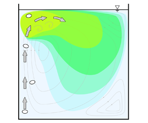
This prompts us to propose a third potential mechanism for the transition in our flow. The mechanism we propose is based on the observation that the velocity fluctuations were strongest near the top of the bubble column, as seen in figure 8. This localisation of the velocity fluctuations suggests that disturbances are generated in the region where the bubbles approach the free surface and that these disturbances are then carried by the mean circulation to the bulk region of the tank. In other words, figure 8 suggests the transition is due to a convective instability above the bubble column. This convection is depicted schematically by step 4 in figure 9.
Colour maps showing the intensity of velocity fluctuations, standard deviation normalised by the mean, in the  $x$ and $y$ components for ${Ra}=3.4\times 10^4$. The $x$–
$x$– $y$ plane projection of the mean velocity field is shown as arrows. Both for the fluctuations and for the mean field, data are averaged in the $z$ direction. Black circles represent the approximate location of the bubble column.

A schematic diagram showing the mechanism proposed for the observed transition. Arrows represent the impinging jet of raising fluid, and coloured regions schematically represent areas with varying intensities of velocity fluctuations with intensity decreasing from yellow to light blue.

The question that still remains is what triggers the velocity fluctuations observed at the top of the bubble column. Since our measurements were concentrated only on the bulk of the tank, the region where the bubbles reach the free surface is inaccessible to our quantitative assessment. Hence, we presently suggest a mechanism aligned with the existing data, deferring quantitative validation for future investigations. Thus, a mechanism that could trigger the velocity fluctuations in this region is related to the interaction of the rising fluid in the bubble column region with the free surface. The bubble column forces the fluid in its vicinity upwards, driving a vertical stream of water in this region (steps 1 and 2 in figure 9). This rising jet of fluid then impinges on the free surface, imposing it to make a sharp turn (step 3 in figure 9). The turning of the jet thus introduces vorticity which increases with the bubble injection rate. Therefore, the main source of the instability scenario proposed here is the jet impingement on the free surface and its consequent turning, which amplifies vorticity fluctuations within the rising jet. It is well-documented that jet impingement is susceptible to instability, characterised by the emission of vortex pairs from the impingement region and the amplification of initial disturbances within the jet (e.g. Popiel & Trass (Reference Popiel and Trass1991), Tsubokura et al. (Reference Tsubokura, Kobayashi, Taniguchi and Jones2003) and citations therein). This mechanism is consistent with the flow visualisations in figure 1(d–f) and in supplementary movies 1 and 2, where spiralling particle trajectories emanating from the region in which the bubble column reaches the free surface and helical trajectories can be clearly seen across the free surface and the wall opposite to the bubble column. Indeed, the mechanism just described aligns best with our flow visualisations, and warrants further quantitative analysis in future investigations.
6. Discussion and conclusions
This work have presented an experimental characterisation of the flow driven by buoyant bubbles rising at moderate Reynolds numbers in a water tank. The flow was studied through quantitative 3D-PTV measurements and flow visualisations, as the system was driven at Rayleigh numbers covering roughly two orders of magnitude. Despite the seemingly simple settings, the flow presents complex dynamics. The first feature is the appearance of a tank-scale circulation. The circulation is balanced by the wall friction, which leads to a power law of  ${Re}\sim {Ra}^{2/5}$ (3.5), as confirmed in our measurements (figure 3). Due to the discrete nature of the forcing the circulation is unsteady even at the lowest Rayleigh number used as it exhibits slow temporal fluctuations with an intensity of approximately 30 % of the mean circulation. Furthermore, the topology of the mean circulation was seen, through flow visualisations, to be rather complex, three dimensional and lacking symmetry with respect to $z$. We believe that this lack of symmetry is responsible for a lack of ergodicity in our flow, which manifested itself in the scatter around the trend observed in figure 3(a). As the Rayleigh number was increased by increasing the bubble injection rate, a transition to a state of fluctuation growth occurred. Above this transition, the energy of the fluctuating flow component grew with the Rayleigh number scaling of ${Ra}^\gamma$ with $\gamma =1.05\pm 0.05$, reaching approximately 150 % of the mean circulating flow energy at the highest Rayleigh number tested. Increasing Rayleigh number above the transition caused increasing fractions of the fluctuation energy to appear in smaller scales; this coincided with the emergence of helical trajectories in the flow visualisations (figure 3(e,f), and in supplementary movies 1 and 2). Notably, despite the observed instability and growth of fluctuations, turbulence was never fully developed in the sense that no inertial range was found in the structure functions (figure 5). This is in concurrence with the relatively low Reynolds numbers in our experiment.
Despite its apparent simplicity in configuration, this system has the capacity to generate intricate physical behaviours. First, the forcing applied on the flow is ‘free’ in the sense that the flow in the tank has a feedback effect on the bubble column. This could change the system behaviour in complex, unexpected ways, as for example was observed by the scatter of the  $A$ value in figure 3. An analogous kind of feedback loop occurs in cavity flows, where interactions of the free shear layer with the flow impingement on the downstream cavity wall is known to produce coherent acoustic oscillations through a feedback mechanism (Rockwell & Naudascher Reference Rockwell and Naudascher1978). Second, the forcing in our bubble system is applied in a temporally discrete fashion, so oscillations and fluctuations can occur already at very low Reynolds numbers. Furthermore, the fluid agitation in the bubble wakes, that is known to lead to pseudo-turbulence states in bubbly flows (Risso Reference Risso2018) could make the problem even more difficult, as energy is injected to the system at various scales. All in all, these issues are expected to lead to significant difficulties should low-order modelling of this system be attempted.
The system under investigation in this study presents several interesting features, including flow oscillations and fluctuations at low Reynolds numbers, and a transition to a regime of highly disturbed flow. The potential to manipulate these features could be utilised in applications such as bio-reactors used for growing aquatic organisms, such as plankton. In these systems, bubbles play a crucial role in oxygenation and nutrient mixing. By precisely adjusting air flow rates, one could potentially achieve desired mixing rates while ensuring that the flow remains below the transition point. This strategy could be leveraged to prevent excessive flow fluctuations that might harm the organisms being cultivated in the reactor. For the flow conditions tested here, velocity fluctuations are moderate and representative of turbulence levels in the ocean (Franks et al. Reference Franks, Inman, MacKinnon, Alford and Waterhouse2021). This set-up could thus also serve as a platform to systematically investigate interactions between turbulence and phytoplankton or zooplankton.
There exist various parameters beyond the airflow rate utilised in this study that could impact the behaviour of the system, including the bubble size, the tank aspect ratio and the bubble injector position. Indeed, studying the phase space of this system holds potential for other flow regimes to be discovered. Several questions, such as verifying the mechanism behind the observed transition, remain open for future research.
Supplementary movies
Supplementary movies are available at https://doi.org/10.1017/jfm.2024.712.
Acknowledgements
We are grateful to M.N. Halic, S. Brizzolara and A. Gambino for fruitful discussions. R.S. was a Rothschild postdoctoral fellow during the initial parts of this work.
Declaration of interests
The authors report no conflict of interest.


 Open access