


1. Introduction and data sets used
Interest in characterising the normal stress of turbulent fluctuations and its relationship to large-scale eddies has significantly increased over the last five to ten years. Two models have been proposed to represent the trends for normal stresses of turbulence in wall-bounded flows, and they are the focus of recent research and publications. Nagib, Vinuesa & Hoyas (Reference Nagib, Vinuesa and Hoyas2024) used indicator functions with carefully selected direct numerical simulation (DNS) data for channel and pipe flows to examine the validity of both models and their potential applicable ranges. The indicator function approach was also tried for experimental data by Monkewitz (Reference Monkewitz2023). The current work is also motivated by recent findings regarding an extended overlap region of the mean velocity profile for wall-bounded turbulent flows by Monkewitz & Nagib (Reference Monkewitz and Nagib2023), revealing that not all such flows exhibit a pure logarithmic profile and a linear term of the same order should be considered. One potential implication from the additional linear term in the mean flow is that it would require eddies that do not strictly scale with their distance from the wall in this overlap region.
One model is based on the attached-eddy concept described by Marusic & Monty (Reference Marusic and Monty2019). Here, we will refer to this model as the ‘wall-scaled eddies model’ or simply the ‘logarithmic trend’ model. For the streamwise normal stress, the trend based on this model is given by
 \begin{equation} \small \langle u^+u^+\small\rangle (Y) = B_1 - A_1\ln (Y). \end{equation}
The outer-scaled distance from the wall $Y$
is defined as
$Y$
is defined as $y/R$
for the pipe flow and as
$y/R$
for the pipe flow and as $y/\delta$
for the zero-pressure-gradient (ZPG) turbulent boundary layer data, where
$y/\delta$
for the zero-pressure-gradient (ZPG) turbulent boundary layer data, where $R$
is the pipe radius and
$R$
is the pipe radius and $\delta$
is the boundary layer thickness. The
$\delta$
is the boundary layer thickness. The $\delta$
used here is the same as that used by Samie et al. (Reference Samie, Marusic, Hutchins, Fu, Fan, Hultmark and Smits2018), which was based on the composite profile proposed by Chauhan, Monkewitz & Nagib (Reference Chauhan, Monkewitz and Nagib2009). Recently, Baxerras, Vinuesa & Nagib (Reference Baxerres, Vinuesa and Nagib2024) compared values based on this composite profile for a wide range of favourable, adverse and ZPG boundary layers, and consistently found
$\delta$
used here is the same as that used by Samie et al. (Reference Samie, Marusic, Hutchins, Fu, Fan, Hultmark and Smits2018), which was based on the composite profile proposed by Chauhan, Monkewitz & Nagib (Reference Chauhan, Monkewitz and Nagib2009). Recently, Baxerras, Vinuesa & Nagib (Reference Baxerres, Vinuesa and Nagib2024) compared values based on this composite profile for a wide range of favourable, adverse and ZPG boundary layers, and consistently found $\delta /\delta _{99} \approx 1.25$
.
$\delta /\delta _{99} \approx 1.25$
.
Recent publications by Chen & Sreenivasan (Reference Chen and Sreenivasan2022, Reference Chen and Sreenivasan2023) on bounded dissipation introduce an alternative model, which we will refer to as the ‘power trend’ model. This model is represented by the following relation for the streamwise normal stress:
 \begin{equation} \big \langle u^+u^+\big \rangle (Y) = \alpha _1 - \beta _1\,(Y)^{0.25}. \end{equation}
Both models contain two parameters and, in addition, the power trend and its exponent are based on the bounding of dissipation near the wall at infinite Reynolds number. The subscript ‘ $1$
’ represents the streamwise component of the normal stresses of turbulence. Analysing velocity spectra obtained in pipe flow using direct numerical simulations, Pirozzoli (Reference Pirozzoli2024) suggests that the dissipation rate of the streamwise velocity reaches a limiting value of
$1$
’ represents the streamwise component of the normal stresses of turbulence. Analysing velocity spectra obtained in pipe flow using direct numerical simulations, Pirozzoli (Reference Pirozzoli2024) suggests that the dissipation rate of the streamwise velocity reaches a limiting value of $0.28$
for high
$0.28$
for high $Re_\tau$
. Hence, it is worthwhile to parametrically test for the power of the exponent in (1.2).
$Re_\tau$
. Hence, it is worthwhile to parametrically test for the power of the exponent in (1.2).
Agreement with the logarithmic trend is often evaluated in the literature, particularly with comparison to experimental data, by fitting a straight line over a segment of the normal stress data on a semi-log plot; examples are found from Marusic et al. (Reference Marusic, Monty, Hultmark and Smits2013), and more recently from Diwan & Morrison (Reference Diwan and Morrison2021) and Hwang, Hutchins & Marusic (Reference Hwang, Hutchins and Marusic2022). This approach makes it challenging to assess the accuracy and ranges of validity of the models, particularly due to the often sparse logarithmic spacing of results in the fitting and outer regions, as well as the limited accuracy of experimental data. For the $0.25$
-power trend, agreement with data is typically tested by iteratively adjusting the two parameters
$0.25$
-power trend, agreement with data is typically tested by iteratively adjusting the two parameters $\alpha _1$
and
$\alpha _1$
and $\beta _1$
, seeking minimum deviations over the widest possible range of distances from the wall in a fitting region between wall- and outer-flow parts. Equations (1.1) and (1.2) are independent of Reynolds number and
$\beta _1$
, seeking minimum deviations over the widest possible range of distances from the wall in a fitting region between wall- and outer-flow parts. Equations (1.1) and (1.2) are independent of Reynolds number and $Re_\tau$
enters into them through the inner limit of the fitting procedure in
$Re_\tau$
enters into them through the inner limit of the fitting procedure in $y^+$
. This is the main reason we use
$y^+$
. This is the main reason we use $Y = y^+ / Re_\tau$
for distance to the wall almost exclusively here.
$Y = y^+ / Re_\tau$
for distance to the wall almost exclusively here.
In the case of DNS data, indicator functions analogous to those used with mean velocity profiles by Monkewitz & Nagib (Reference Monkewitz and Nagib2023) were identified as having the best potential for normal stress analysis and were favoured by Nagib et al. (Reference Nagib, Vinuesa and Hoyas2024). However, just like with mean velocity, these indicator functions require taking derivatives of the discrete normal stress profiles. This approach is often unsuitable for most experimental data in the literature due to limited spatial resolution and experimental accuracy, which hamper the ability to obtain accurate derivatives of the profiles. The current work aims to develop a method for assessing the proposed relations using two of the most well-documented and reliable experimental results in zero-pressure-gradient boundary layers and pipe flows, as provided by Hultmark et al. (Reference Hultmark, Vallikivi, Bailey and Smits2012) and Samie et al. (Reference Samie, Marusic, Hutchins, Fu, Fan, Hultmark and Smits2018), respectively.
A new approach is introduced here and successfully implemented with these two experimental data sets over a ‘fitting region’ defined for this work by the following. Using accurate measurements with established uncertainty limits throughout the fitting region, the method is based on a normalisation scheme that uses the respective trend relations with adjustable parameters within defined bounds. The bounds are selected to establish a fitting region for each model between inner and outer flow parts. To meet this criterion, the current assessment of the streamwise normal stress primarily focuses on regions of the flow beyond the very near wall, specifically targeting ranges of $y^+$
larger than 400, which correspond to a nominal outer variable range in the case of ZPG of
$y^+$
larger than 400, which correspond to a nominal outer variable range in the case of ZPG of $0.004 \lessapprox Y \lessapprox 0.2$
for the logarithmic trend and
$0.004 \lessapprox Y \lessapprox 0.2$
for the logarithmic trend and $0.004 \lessapprox Y \lessapprox 0.4$
for the power trend in the
$0.004 \lessapprox Y \lessapprox 0.4$
for the power trend in the $Re_\tau$
range examined. For the logarithmic trend of normal stresses, the traditionally used overlap region extends up to
$Re_\tau$
range examined. For the logarithmic trend of normal stresses, the traditionally used overlap region extends up to $Y$
of
$Y$
of $0.1$
or
$0.1$
or $0.15$
, which is reflected in the mean velocity profiles. We extended the range for our examination of the data against the two models for a more thorough assessment. The inner-scaled wall distance is defined as
$0.15$
, which is reflected in the mean velocity profiles. We extended the range for our examination of the data against the two models for a more thorough assessment. The inner-scaled wall distance is defined as $y^+ = y u_\tau /\nu$
, where
$y^+ = y u_\tau /\nu$
, where $Re_\tau$
is equal to
$Re_\tau$
is equal to $u_\tau \delta /\nu$
for ZPG flows and
$u_\tau \delta /\nu$
for ZPG flows and $u_\tau R/\nu$
for pipes. The fluid kinematic viscosity
$u_\tau R/\nu$
for pipes. The fluid kinematic viscosity $\nu$
is determined from the fluid temperature and
$\nu$
is determined from the fluid temperature and $u_\tau$
is the wall friction velocity
$u_\tau$
is the wall friction velocity $\sqrt {\tau _w/\rho }$
, with
$\sqrt {\tau _w/\rho }$
, with $\tau _w$
measured by pressure drop in the fully developed pipe flow, and directly using oil-film interferometry (OFI) in the ZPG experiment. The experiments of Samie et al. (Reference Samie, Marusic, Hutchins, Fu, Fan, Hultmark and Smits2018) included values of
$\tau _w$
measured by pressure drop in the fully developed pipe flow, and directly using oil-film interferometry (OFI) in the ZPG experiment. The experiments of Samie et al. (Reference Samie, Marusic, Hutchins, Fu, Fan, Hultmark and Smits2018) included values of $u_\tau$
from both the direct measurement by OFI and by the composite profile approach of Chauhan et al. (Reference Chauhan, Monkewitz and Nagib2009). We used the results based on
$u_\tau$
from both the direct measurement by OFI and by the composite profile approach of Chauhan et al. (Reference Chauhan, Monkewitz and Nagib2009). We used the results based on $u_\tau$
values measured with OFI.
$u_\tau$
values measured with OFI.
It is important to establish the regions of validity for each of the two models. This will be discussed in § 5. We will focus initially on comparing the two models of (1.1) and (1.2) in the intermediate or overlap region where nearly all the literature has evaluated them with experimental or computational data as shown by Marusic et al. (Reference Marusic, Monty, Hultmark and Smits2013), Diwan & Morrison (Reference Diwan and Morrison2021), Hwang et al. (Reference Hwang, Hutchins and Marusic2022), Monkewitz (Reference Monkewitz2023) and Chen & Sreenivasan (Reference Chen and Sreenivasan2024). For the different wall-bounded turbulent flows, the outer part of the flow can differ a great deal from boundary layers to duct flows such as in channels and pipes. We hope that the approach described and tested in this work will reveal some differences among these fitting regions, although the near-wall flow may be quite similar. For these high- $Re_\tau$
experiments, the fitting region is selected to incorporate the majority of the inner part of the overlap region between inner and outer flow parts as defined by each model, while extending to wall distances in outer variable
$Re_\tau$
experiments, the fitting region is selected to incorporate the majority of the inner part of the overlap region between inner and outer flow parts as defined by each model, while extending to wall distances in outer variable $Y$
to include the range of agreement between the data and each model.
$Y$
to include the range of agreement between the data and each model.
Initial evaluations for the power trend model were made with the exponent of $0.25$
based on the bounded dissipation results. We also tested other exponents in the range from
$0.25$
based on the bounded dissipation results. We also tested other exponents in the range from $0.2$
to
$0.2$
to $0.32$
. For ZPG turbulent boundary layers, data from the Melbourne large wind tunnel by Marusic et al. (Reference Marusic, Chauhan, Kulandaivelu and Hutchins2015) and Samie et al. (Reference Samie, Marusic, Hutchins, Fu, Fan, Hultmark and Smits2018) were used, with emphasis on the recent results using more advanced hot wire anemometers that provided better spatial resolution.
$0.32$
. For ZPG turbulent boundary layers, data from the Melbourne large wind tunnel by Marusic et al. (Reference Marusic, Chauhan, Kulandaivelu and Hutchins2015) and Samie et al. (Reference Samie, Marusic, Hutchins, Fu, Fan, Hultmark and Smits2018) were used, with emphasis on the recent results using more advanced hot wire anemometers that provided better spatial resolution.
The earlier measurements of Marusic et al. (Reference Marusic, Chauhan, Kulandaivelu and Hutchins2015) used miniature conventional hot-wire sensors. Similarly for the normal stress data from the Princeton Superpipe facility, the more recent data by NSTAP hot-wire sensors with a smaller sensor length from Hultmark et al. (Reference Hultmark, Vallikivi, Bailey and Smits2012) were used.
For the DNS results, the various channel and pipe flows data recently examined with the indicator functions approach by Nagib et al. (Reference Nagib, Vinuesa and Hoyas2024) are used to re-evaluate both trend models by the new method. These results were also compared with the results for higher $Re_\tau$
from the two experiments examined in the next section.
$Re_\tau$
from the two experiments examined in the next section.
Streamwise turbulence stress versus inner-scaled wall distance for different $Re_\tau$
values from Marusic et al. (Reference Marusic, Chauhan, Kulandaivelu and Hutchins2015) and Samie et al. (Reference Samie, Marusic, Hutchins, Fu, Fan, Hultmark and Smits2018) ZPG (open symbols) data with 0.25-power parameters (9.2
$Re_\tau$
values from Marusic et al. (Reference Marusic, Chauhan, Kulandaivelu and Hutchins2015) and Samie et al. (Reference Samie, Marusic, Hutchins, Fu, Fan, Hultmark and Smits2018) ZPG (open symbols) data with 0.25-power parameters (9.2 $\pm$
0.22, 10.1
$\pm$
0.22, 10.1 $\pm$
0.13) and logarithmic parameters (−1.26, 1.93
$\pm$
0.13) and logarithmic parameters (−1.26, 1.93 $\pm$
0.05); C1 = 400 and C2 = 5000.
$\pm$
0.05); C1 = 400 and C2 = 5000.

2. Evaluating logarithmic and quarter-power relations
The collection of the streamwise normal stress profiles from the Melbourne ZPG experiments and the Princeton Superpipe are plotted against the logarithm of the inner-scale wall distance in figures 1 and 2, respectively. The logarithmic trend is represented by solid straight lines using (1.1) with typical $A_1$
and
$A_1$
and $B_1$
values for ZPG in figure 1 and for pipe flows in figure 2; with corresponding parameter values listed in the captions of all relevant figures in the format (
$B_1$
values for ZPG in figure 1 and for pipe flows in figure 2; with corresponding parameter values listed in the captions of all relevant figures in the format ( $A_1$
,
$A_1$
, $B_1$
). It is noted that in this paper, we consider the logarithmic relation for the streamwise normal stresses at face value, as it is predominantly considered in the literature. Some potential exists to improve on the logarithmic relation by including nonlinear scaling from the wall and viscous effects. More recent work by Baars & Marusic (Reference Baars and Marusic2020) and Deshpande, Monty & Marusic (Reference Deshpande, Monty and Marusic2021) has shown that a pure logarithmic relationship relies on first isolating the very-large-scale or ‘superstructure’ contributions that do not scale with their distance from the wall.
$B_1$
). It is noted that in this paper, we consider the logarithmic relation for the streamwise normal stresses at face value, as it is predominantly considered in the literature. Some potential exists to improve on the logarithmic relation by including nonlinear scaling from the wall and viscous effects. More recent work by Baars & Marusic (Reference Baars and Marusic2020) and Deshpande, Monty & Marusic (Reference Deshpande, Monty and Marusic2021) has shown that a pure logarithmic relationship relies on first isolating the very-large-scale or ‘superstructure’ contributions that do not scale with their distance from the wall.
Streamwise turbulence stress versus inner-scaled wall distance for different $Re_\tau$
values from Hultmark et al. (Reference Hultmark, Vallikivi, Bailey and Smits2012) superpipe data with 0.25-power parameters (9.3
$Re_\tau$
values from Hultmark et al. (Reference Hultmark, Vallikivi, Bailey and Smits2012) superpipe data with 0.25-power parameters (9.3 $\pm$
0.13, 10.0
$\pm$
0.13, 10.0 $\pm$
0.0.06), and logarithmic parameters (−1.26, 1.6
$\pm$
0.0.06), and logarithmic parameters (−1.26, 1.6 $\pm$
0.17); C1 = 400 and C2 = 5000.
$\pm$
0.17); C1 = 400 and C2 = 5000.

The power trend fits, (1.2), are depicted using dotted lines in figures 1 and 2, with both trends using colours corresponding to the data symbols for each $Re_\tau$
. Typical values of
$Re_\tau$
. Typical values of $\alpha _1$
and
$\alpha _1$
and $\beta _1$
as reported in the literature are used. The format in the captions of all relevant figures for the power trend coefficients is (
$\beta _1$
as reported in the literature are used. The format in the captions of all relevant figures for the power trend coefficients is ( $\beta _1$
,
$\beta _1$
, $\alpha _1$
). In the case of the Superpipe data, the parameters were slightly adjusted to optimise their fit for some of the
$\alpha _1$
). In the case of the Superpipe data, the parameters were slightly adjusted to optimise their fit for some of the $Re_\tau$
cases, over the very wide range of Reynolds numbers, and the standard deviation for each parameter is also listed in the caption following the corresponding mean value. The green and blue bars near the bottom of each figure represent the apparent agreement between the data and the trend models corresponding to logarithmic and power relations, respectively. Two parts of each bar with different shades of its colour are used to identify the apparent range of agreement with the corresponding trend for normal stress profiles with typical lower and higher
$Re_\tau$
cases, over the very wide range of Reynolds numbers, and the standard deviation for each parameter is also listed in the caption following the corresponding mean value. The green and blue bars near the bottom of each figure represent the apparent agreement between the data and the trend models corresponding to logarithmic and power relations, respectively. Two parts of each bar with different shades of its colour are used to identify the apparent range of agreement with the corresponding trend for normal stress profiles with typical lower and higher $Re_\tau$
values.
$Re_\tau$
values.
The thick grey lines are used to provide a visual indication of the boundary between the near-wall and fitting region of the flow, where the validity of the relation will be evaluated more carefully in the following figures. Using the information in figure 6 of Nagib et al. (Reference Nagib, Vinuesa and Hoyas2024) and identifying the fitting region as that to the right of the minimum peak in the profiles of turbulent stress gradient divided by viscous stress gradient, the following relation for the grey lines is used: $y^+ = C_1 (Re_\tau / C_2)^{0.5}$
. This relation recognises the square root dependence observed in figure 6 of Nagib et al. (Reference Nagib, Vinuesa and Hoyas2024). A conservative value of
$y^+ = C_1 (Re_\tau / C_2)^{0.5}$
. This relation recognises the square root dependence observed in figure 6 of Nagib et al. (Reference Nagib, Vinuesa and Hoyas2024). A conservative value of $C_1 = 400$
corresponding to
$C_1 = 400$
corresponding to $C_2 = 5000$
is used. This selects
$C_2 = 5000$
is used. This selects $y^+=400$
as a conservative lower limit of the fitting region for
$y^+=400$
as a conservative lower limit of the fitting region for $Re_\tau = 5000$
.
$Re_\tau = 5000$
.
The method introduced here is intended to have a more quantitative evaluation than that used in figures 1 and 2, or in most of the previous attempts in the literature. For each model, the normal stress profile measurements for a given $Re_\tau$
are divided at each data point by the corresponding value from the model and plotted against inner-scaled distance from the wall
$Re_\tau$
are divided at each data point by the corresponding value from the model and plotted against inner-scaled distance from the wall $y^+$
on a log scale or the outer-scaled distance from the wall
$y^+$
on a log scale or the outer-scaled distance from the wall $Y$
on a linear scale. To compare the two models, the resulting graphs for the logarithmic model are always placed in panel (a) of the composite figures 3–6, while the power model is shown in panel (b). The values of the parameters for both models (
$Y$
on a linear scale. To compare the two models, the resulting graphs for the logarithmic model are always placed in panel (a) of the composite figures 3–6, while the power model is shown in panel (b). The values of the parameters for both models ( $A_1$
,
$A_1$
, $B_1$
) and (
$B_1$
) and ( $\beta _1$
,
$\beta _1$
, $\alpha _1$
) are listed in the captions for each figure in this format. When various
$\alpha _1$
) are listed in the captions for each figure in this format. When various $Re_\tau$
cases required slight adjustments in these parameters, the standard deviation of the full range of
$Re_\tau$
cases required slight adjustments in these parameters, the standard deviation of the full range of $Re_\tau$
values is again listed after the mean value. Based on experience with the entire experimental data sets used here and recognising the uncertainties in the measurement of the streamwise normal stress using hot wire sensors, we selected a maximum deviation from the exact agreement ratio of
$Re_\tau$
values is again listed after the mean value. Based on experience with the entire experimental data sets used here and recognising the uncertainties in the measurement of the streamwise normal stress using hot wire sensors, we selected a maximum deviation from the exact agreement ratio of $1.0\,\%$ $\pm 2\, \%$
. In the next figures, this range of acceptable model representation of the data is depicted with horizontal grey bands.
$\pm 2\, \%$
. In the next figures, this range of acceptable model representation of the data is depicted with horizontal grey bands.
Streamwise turbulence stress normalised by both fitting relations versus inner-scaled wall distance for ZPG data of Marusic et al. (Reference Marusic, Chauhan, Kulandaivelu and Hutchins2015) and Samie et al. (Reference Samie, Marusic, Hutchins, Fu, Fan, Hultmark and Smits2018) for different $Re_\tau$
values: (a) using (1.1) with logarithmic parameters (−1.26, 1.93
$Re_\tau$
values: (a) using (1.1) with logarithmic parameters (−1.26, 1.93 $\pm$
0.05); (b) using (1.2) with 0.25-power parameters (9.2
$\pm$
0.05); (b) using (1.2) with 0.25-power parameters (9.2 $\pm$
0.22, 10.1
$\pm$
0.22, 10.1 $\pm$
0.13).
$\pm$
0.13).

Figure 3 summarises the evaluation of the ZPG data using the method described in the previous paragraph. The vertical axis represents the ratio between the measured streamwise normal stress and the expected values based on the fitting trend relation, $\langle u^+u^+ \rangle / \langle u^+u^+ \rangle _{fitting}$
. Just as in figures 1 and 2, the green and blue bars near the bottom identify the range of validity with the respective fitting trend, but more quantitatively now with the help of the horizontal grey bars establishing agreement of the ratio of the data to the relation at the same location of wall distance with
$\langle u^+u^+ \rangle / \langle u^+u^+ \rangle _{fitting}$
. Just as in figures 1 and 2, the green and blue bars near the bottom identify the range of validity with the respective fitting trend, but more quantitatively now with the help of the horizontal grey bars establishing agreement of the ratio of the data to the relation at the same location of wall distance with $1.0 \pm 0.02$
. A similar evaluation is carried out in figure 4 using the outer scaled distance
$1.0 \pm 0.02$
. A similar evaluation is carried out in figure 4 using the outer scaled distance $Y$
on a linear horizontal axis. In figures 5 and 6, the two sets of evaluations versus
$Y$
on a linear horizontal axis. In figures 5 and 6, the two sets of evaluations versus $y^+$
and
$y^+$
and $Y$
are repeated for the Superpipe data. We find from these four figures that the lower limit of fitting of validity in inner variables for both logarithmic and power relations changes weakly for
$Y$
are repeated for the Superpipe data. We find from these four figures that the lower limit of fitting of validity in inner variables for both logarithmic and power relations changes weakly for $Re_\tau \gtrapprox 10\,000$
within the scatter of the results.
$Re_\tau \gtrapprox 10\,000$
within the scatter of the results.
ZPG data. Same as figure 3 but with outer-scaled wall distance.

Streamwise turbulence stress normalised by both fitting relations versus inner-scaled wall distance for Superpipe data of Hultmark et al. (Reference Hultmark, Vallikivi, Bailey and Smits2012) for different $Re_\tau$
values: (a) using (1.1) with logarithmic parameters (−1.26, 1.6
$Re_\tau$
values: (a) using (1.1) with logarithmic parameters (−1.26, 1.6 $\pm$
0.17); (b) sing (1.2) with 0.25-power parameters (9.3
$\pm$
0.17); (b) sing (1.2) with 0.25-power parameters (9.3 $\pm$
0.13, 10.0
$\pm$
0.13, 10.0 $\pm$
0.06).
$\pm$
0.06).

Examining the minimum peak in both parts of figure 6 of Nagib et al. (Reference Nagib, Vinuesa and Hoyas2024) and relating them to an arbitrary fractional power of $Re_\tau$
with an adjustable proportionality coefficient, we find that a best fit is
$Re_\tau$
with an adjustable proportionality coefficient, we find that a best fit is $y^+ = 1.5 \cdot Re_\tau ^{0.5}$
. In the figure, this minimum peak is readily identified with a transition between the near wall flow and the overlap region over the range
$y^+ = 1.5 \cdot Re_\tau ^{0.5}$
. In the figure, this minimum peak is readily identified with a transition between the near wall flow and the overlap region over the range $1000 \lt Re_\tau \lt 16\,000$
based on DNS of channel flow and, therefore, readily with
$1000 \lt Re_\tau \lt 16\,000$
based on DNS of channel flow and, therefore, readily with $y^+_{in}$
.
$y^+_{in}$
.
Consistent with the analysis of Klewicki, Fife & Wei (Reference Klewicki, Fife and Wei2009) and Nagib et al. (Reference Nagib, Vinuesa and Hoyas2024), we will thus consider $y^+_{in} \sim (Re_\tau )^{0.5}$
, with the provision that
$y^+_{in} \sim (Re_\tau )^{0.5}$
, with the provision that $y^+_{in} \gtrapprox 400$
for the ZPG and Superpipe data. This corresponds to
$y^+_{in} \gtrapprox 400$
for the ZPG and Superpipe data. This corresponds to $0.004 \lessapprox Y_{in} \lessapprox 0.04$
for the range of
$0.004 \lessapprox Y_{in} \lessapprox 0.04$
for the range of $Re_\tau$
considered here. The upper limit of fitting validity in outer variables
$Re_\tau$
considered here. The upper limit of fitting validity in outer variables $Y_{out}$
, for both logarithmic and power relations, appears to be independent of
$Y_{out}$
, for both logarithmic and power relations, appears to be independent of $Re_\tau$
in the Superpipe and ZPG data; see figures 4, 6 and 7. We find bounds for the logarithmic relation that incorporate the region of the flow where the classical pure-logarithmic relation of the mean velocity profiles can be identified (see region
$Re_\tau$
in the Superpipe and ZPG data; see figures 4, 6 and 7. We find bounds for the logarithmic relation that incorporate the region of the flow where the classical pure-logarithmic relation of the mean velocity profiles can be identified (see region $Y \lessapprox 0.1$
in figure 4 of Baxerras et al. Reference Baxerres, Vinuesa and Nagib2024 and figure 7 of Monkewitz & Nagib Reference Monkewitz and Nagib2023), and therefore, consistent with the wall-scaled (attached) eddy model (Marusic et al. Reference Marusic, Monty, Hultmark and Smits2013). However, it is significant to note that the upper limit of fitting validity in outer variable
$Y \lessapprox 0.1$
in figure 4 of Baxerras et al. Reference Baxerres, Vinuesa and Nagib2024 and figure 7 of Monkewitz & Nagib Reference Monkewitz and Nagib2023), and therefore, consistent with the wall-scaled (attached) eddy model (Marusic et al. Reference Marusic, Monty, Hultmark and Smits2013). However, it is significant to note that the upper limit of fitting validity in outer variable $Y_{out}$
is considerably higher for the power relation compared with the logarithmic relation. For ZPG,
$Y_{out}$
is considerably higher for the power relation compared with the logarithmic relation. For ZPG, $Y_{out}$
is
$Y_{out}$
is $0.39$
compared with
$0.39$
compared with $0.22$
and for the Superpipe data is
$0.22$
and for the Superpipe data is $0.5$
versus
$0.5$
versus $0.27$
; see figures 4 and 6. The corresponding limits in
$0.27$
; see figures 4 and 6. The corresponding limits in $y^+$
values are easily obtained from the
$y^+$
values are easily obtained from the $Re_\tau$
conditions. For example, when
$Re_\tau$
conditions. For example, when $Re_\tau \approx 20\,000$
, the logarithmic trend is found only up to
$Re_\tau \approx 20\,000$
, the logarithmic trend is found only up to $y^+\approx 5000$
, while the power relation extends the agreement to
$y^+\approx 5000$
, while the power relation extends the agreement to $y^+\approx 9000$
.
$y^+\approx 9000$
.
Superpipe data. Same as figure 5 but with outer-scaled wall distance.

Streamwise turbulence stress normalised by both fitting relations versus outer-scaled wall distance for different $Re_\tau$
values. (a) ZPG data of Samie et al. (Reference Samie, Marusic, Hutchins, Fu, Fan, Hultmark and Smits2018) with 0.28-power parameters (8.9
$Re_\tau$
values. (a) ZPG data of Samie et al. (Reference Samie, Marusic, Hutchins, Fu, Fan, Hultmark and Smits2018) with 0.28-power parameters (8.9 $\pm$
0.21, 9.6
$\pm$
0.21, 9.6 $\pm$
0.26). (b) ZPG data of Samie et al. (Reference Samie, Marusic, Hutchins, Fu, Fan, Hultmark and Smits2018) with 0.22-power parameters (9.6
$\pm$
0.26). (b) ZPG data of Samie et al. (Reference Samie, Marusic, Hutchins, Fu, Fan, Hultmark and Smits2018) with 0.22-power parameters (9.6 $\pm$
0.23, 10.6
$\pm$
0.23, 10.6 $\pm$
0.13).
$\pm$
0.13).

Streamwise turbulence stress normalised by both fitting relations versus outer-scaled wall distance for different $Re_\tau$
values. (a) Superpipe data of Hultmark et al. (Reference Hultmark, Vallikivi, Bailey and Smits2012) with 0.28-power parameters (8.6
$Re_\tau$
values. (a) Superpipe data of Hultmark et al. (Reference Hultmark, Vallikivi, Bailey and Smits2012) with 0.28-power parameters (8.6 $\pm$
0.1, 9.10
$\pm$
0.1, 9.10 $\pm$
0.23). (b) Superpipe data of Hultmark et al. (Reference Hultmark, Vallikivi, Bailey and Smits2012) with 0.22-power parameters (9.8
$\pm$
0.23). (b) Superpipe data of Hultmark et al. (Reference Hultmark, Vallikivi, Bailey and Smits2012) with 0.22-power parameters (9.8 $\pm$
0.1, 10.5
$\pm$
0.1, 10.5 $\pm$
0.26).
$\pm$
0.26).

3. Power-relation exponent, intermittency effects and comparison to DNS
In figures 7 and 8, the variation of the exponent of the power model is tested. Panel (a) of each figure displays the evaluation of the experimental data by a power relation with $0.28$
exponent, while panel (b) uses an exponent of
$0.28$
exponent, while panel (b) uses an exponent of $0.22$
. The ZPG data are evaluated in figure 7 and the range of potential impact of the outer intermittency is indicated for reference by a yellow bar near the top of the figure. The function developed by Chauhan et al. (Reference Chauhan, Philip, de Silva, Hutchins and Marusic2014) is used here with all data corrected for intermittency. The function starts at a value of
$0.22$
. The ZPG data are evaluated in figure 7 and the range of potential impact of the outer intermittency is indicated for reference by a yellow bar near the top of the figure. The function developed by Chauhan et al. (Reference Chauhan, Philip, de Silva, Hutchins and Marusic2014) is used here with all data corrected for intermittency. The function starts at a value of $1.0$
from the wall, then decreases to
$1.0$
from the wall, then decreases to $0.96, 0.84, 0.57, 0.24\;\textrm{and}\;0.04$
near the outer scale distances
$0.96, 0.84, 0.57, 0.24\;\textrm{and}\;0.04$
near the outer scale distances $Y$
of
$Y$
of $0.47, 0.55, 0.64, 0.76\;\textrm{and}\;0.89$
, respectively.
$0.47, 0.55, 0.64, 0.76\;\textrm{and}\;0.89$
, respectively.
In contrast, for the Superpipe data shown in figure 8, no influence of intermittency is expected and the agreement with the power relation extends to half the pipe radius. Comparing the results from both ZPG and Superpipe data for power relations with exponents of $0.22$
,
$0.22$
, $0.25$
and
$0.25$
and $0.28$
reveals that an exponent of
$0.28$
reveals that an exponent of $0.28$
represents the data somewhat better than the original
$0.28$
represents the data somewhat better than the original $0.25$
-power relation based on the bounded dissipation model; see also figures 11 and 12. Several other exponents were tested with both data sets, but the
$0.25$
-power relation based on the bounded dissipation model; see also figures 11 and 12. Several other exponents were tested with both data sets, but the $0.28$
appears to yield the best agreement. Applying the intermittency correction used for figure 9 to the
$0.28$
appears to yield the best agreement. Applying the intermittency correction used for figure 9 to the $0.28$
-power relation yields the best agreement with the measured data including for large
$0.28$
-power relation yields the best agreement with the measured data including for large $y^+$
values. The fitting range agreement with the
$y^+$
values. The fitting range agreement with the $0.28$
-power model and the intermittency correction extends to
$0.28$
-power model and the intermittency correction extends to $Y$
over
$Y$
over $0.5$
, consistent with the result of the ratio method in figure 9. A generalisation or extension of the defect power model to explain the
$0.5$
, consistent with the result of the ratio method in figure 9. A generalisation or extension of the defect power model to explain the $0.28$
power found here for channel and ZPG boundary layer flows and suggested through analysis of spectra from pipe data by Pirozzoli (Reference Pirozzoli2024), instead of the
$0.28$
power found here for channel and ZPG boundary layer flows and suggested through analysis of spectra from pipe data by Pirozzoli (Reference Pirozzoli2024), instead of the $0.25$
power of bounded dissipation, appears to be most desirable.
$0.25$
power of bounded dissipation, appears to be most desirable.
Correcting ZPG data for outer intermittency effects using the function of Chauhan et al. (Reference Chauhan, Philip, de Silva, Hutchins and Marusic2014) does not change $Y_{out}$
for the logarithmic relation while extending
$Y_{out}$
for the logarithmic relation while extending $Y_{out}$
for the power relation to approximately
$Y_{out}$
for the power relation to approximately $0.44$
; see figure 9. The correction is simply applied by dividing the ratio
$0.44$
; see figure 9. The correction is simply applied by dividing the ratio $\langle u^+u^+ \rangle / \langle u^+u^+ \rangle _{fitting}$
by the intermittency function that ranges from one at the wall to zero beyond
$\langle u^+u^+ \rangle / \langle u^+u^+ \rangle _{fitting}$
by the intermittency function that ranges from one at the wall to zero beyond $y = \delta$
.
$y = \delta$
.
Streamwise turbulence stress normalised by both fitting relations versus outer-scaled wall distance for different $Re_\tau$
values, with intermittency correction applied. (a) ZPG data of Marusic et al. (Reference Marusic, Chauhan, Kulandaivelu and Hutchins2015) and Samie et al. (Reference Samie, Marusic, Hutchins, Fu, Fan, Hultmark and Smits2018) (open symbols) with logarithmic parameters (–1.26, 1.93
$Re_\tau$
values, with intermittency correction applied. (a) ZPG data of Marusic et al. (Reference Marusic, Chauhan, Kulandaivelu and Hutchins2015) and Samie et al. (Reference Samie, Marusic, Hutchins, Fu, Fan, Hultmark and Smits2018) (open symbols) with logarithmic parameters (–1.26, 1.93 $\pm$
0.05). (b) ZPG data of Marusic et al. (Reference Marusic, Chauhan, Kulandaivelu and Hutchins2015) and Samie et al. (Reference Samie, Marusic, Hutchins, Fu, Fan, Hultmark and Smits2018) (open symbols) with 0.28-power parameters (8.9
$\pm$
0.05). (b) ZPG data of Marusic et al. (Reference Marusic, Chauhan, Kulandaivelu and Hutchins2015) and Samie et al. (Reference Samie, Marusic, Hutchins, Fu, Fan, Hultmark and Smits2018) (open symbols) with 0.28-power parameters (8.9 $\pm$
0.21, 9.6
$\pm$
0.21, 9.6 $\pm$
0.16).
$\pm$
0.16).

In figure 10, DNS results of pipe flow are displayed with dashed lines and channel flow data with continuous lines. Dashed lines with experimental data points identified by solid circles are used for Superpipe data and continuous lines with experimental data points marked by solid circles are used for ZPG data. The colour pattern for the experimental data for different $Re_\tau$
conditions are the same as in earlier figures.
$Re_\tau$
conditions are the same as in earlier figures.
Comparing the ZPG and Superpipe experimental data with DNS data for pipe flow in the range $2000 \lt Re_\tau \lt 6000$
and channel flow in the range
$2000 \lt Re_\tau \lt 6000$
and channel flow in the range $2000 \lt Re_\tau \lt 10\,000$
, reveals general agreement for results of both logarithmic and power relations as displayed in figure 10. The DNS results are based on the recent work of Nagib et al. (Reference Nagib, Vinuesa and Hoyas2024) and all the parameters of the various cases are given in tables included by them.
$2000 \lt Re_\tau \lt 10\,000$
, reveals general agreement for results of both logarithmic and power relations as displayed in figure 10. The DNS results are based on the recent work of Nagib et al. (Reference Nagib, Vinuesa and Hoyas2024) and all the parameters of the various cases are given in tables included by them.
Figure 10 is a further demonstration that, especially near the wall, $Re_\tau \gtrapprox 10\,000$
is required for the two proposed relations to achieve agreement with the streamwise normal stress in the fitting region. This is in contrast to a lower value of
$Re_\tau \gtrapprox 10\,000$
is required for the two proposed relations to achieve agreement with the streamwise normal stress in the fitting region. This is in contrast to a lower value of $Re_\tau \gtrapprox 5\,000$
we find for the indicator functions of the mean velocity profile, as demonstrated by Hoyas et al. (Reference Hoyas, Vinuesa, Schmid and Nagib2024) and figure 1 of Nagib et al. (Reference Nagib, Vinuesa and Hoyas2024).
$Re_\tau \gtrapprox 5\,000$
we find for the indicator functions of the mean velocity profile, as demonstrated by Hoyas et al. (Reference Hoyas, Vinuesa, Schmid and Nagib2024) and figure 1 of Nagib et al. (Reference Nagib, Vinuesa and Hoyas2024).
Streamwise turbulence stress normalised by both fitting relations versus outer-scaled wall distance for different $Re_\tau$
values. (a) Superpipe data of Hultmark et al. (Reference Hultmark, Vallikivi, Bailey and Smits2012) with logarithmic parameters (−1.26, 1.6
$Re_\tau$
values. (a) Superpipe data of Hultmark et al. (Reference Hultmark, Vallikivi, Bailey and Smits2012) with logarithmic parameters (−1.26, 1.6 $\pm$
0.17), ZPG data of Samie et al. (Reference Samie, Marusic, Hutchins, Fu, Fan, Hultmark and Smits2018) (open symbols and dotted lines) and channel DNS data from Nagib et al. (Reference Nagib, Vinuesa and Hoyas2024). (b) Superpipe data of Hultmark et al. (Reference Hultmark, Vallikivi, Bailey and Smits2012) with 0.25-power parameters (9.3
$\pm$
0.17), ZPG data of Samie et al. (Reference Samie, Marusic, Hutchins, Fu, Fan, Hultmark and Smits2018) (open symbols and dotted lines) and channel DNS data from Nagib et al. (Reference Nagib, Vinuesa and Hoyas2024). (b) Superpipe data of Hultmark et al. (Reference Hultmark, Vallikivi, Bailey and Smits2012) with 0.25-power parameters (9.3 $\pm$
0.13, 10.0
$\pm$
0.13, 10.0 $\pm$
0.06), ZPG data of Samie et al. (Reference Samie, Marusic, Hutchins, Fu, Fan, Hultmark and Smits2018) and channel DNS data of Nagib et al. (Reference Nagib, Vinuesa and Hoyas2024).
$\pm$
0.06), ZPG data of Samie et al. (Reference Samie, Marusic, Hutchins, Fu, Fan, Hultmark and Smits2018) and channel DNS data of Nagib et al. (Reference Nagib, Vinuesa and Hoyas2024).

Next, we use the $Re_\tau = 5200$
DNS data of Lee & Moser (Reference Lee and Moser2015) for channel flow and the indicator function for the power trend given by Nagib et al. (Reference Nagib, Vinuesa and Hoyas2024) for
$Re_\tau = 5200$
DNS data of Lee & Moser (Reference Lee and Moser2015) for channel flow and the indicator function for the power trend given by Nagib et al. (Reference Nagib, Vinuesa and Hoyas2024) for $0.25$
power. We focus on the streamwise normal stress and use its indicator function,
$0.25$
power. We focus on the streamwise normal stress and use its indicator function, $\zeta _{uu}$
, defined as
$\zeta _{uu}$
, defined as
 \begin{equation} \zeta _{uu} = y^+\frac {\textrm {d}{\big \langle u_x^+u_x^+\big \rangle }}{\textrm {d}y^+} = Y\frac {\textrm {d}{\big \langle u_x^+u_x^+\big\rangle }}{\textrm {d}Y}. \end{equation}
Finally, to examine whether the power of $1/4$
is reflected in normal stress profiles, the indicator function of the trend of the defect power,
$1/4$
is reflected in normal stress profiles, the indicator function of the trend of the defect power, $\zeta _{uu,BD}$
, based on the bounded-dissipation predictions of (1.1), is defined by
$\zeta _{uu,BD}$
, based on the bounded-dissipation predictions of (1.1), is defined by
 \begin{equation} \zeta _{uu,BD} = 4Re_\tau ^{0.25}(y^+)^{0.75}\frac {\textrm {d}{\Big\langle u^+u^+\Big\rangle }}{\textrm {d}y^+} = 4Y^{0.75}\frac {\textrm {d}{\Big\langle u^+u^+\Big\rangle }}{\textrm {d}Y}. \end{equation}
To evaluate the different values of the exponent using such an indicator function, we use
 \begin{align}\nonumber\\[-24pt]\zeta _{uu,power} = F_{power} \cdot \zeta _{uu,BD}, \end{align}
and select $F_{power}$
for each exponent to bring the indicator functions close to the value of
$F_{power}$
for each exponent to bring the indicator functions close to the value of $-10.5$
reported often in the literature for channel flow (Monkewitz Reference Monkewitz2023; Nagib et al. Reference Nagib, Vinuesa and Hoyas2024) to achieve an optimum visual comparison with increasing value of the exponent. The best agreement, with widest range in
$-10.5$
reported often in the literature for channel flow (Monkewitz Reference Monkewitz2023; Nagib et al. Reference Nagib, Vinuesa and Hoyas2024) to achieve an optimum visual comparison with increasing value of the exponent. The best agreement, with widest range in $Y$
, found with the data for several values of the power exponent is clearly the exponent of
$Y$
, found with the data for several values of the power exponent is clearly the exponent of $0.28$
, for which we select
$0.28$
, for which we select $F_{0.28}$
to match the
$F_{0.28}$
to match the $-10.5$
value for
$-10.5$
value for $\zeta _{uu,power}$
. The results are summarised in figure 11 for four different exponents of the power relation. They reveal that a value of
$\zeta _{uu,power}$
. The results are summarised in figure 11 for four different exponents of the power relation. They reveal that a value of $0.28$
for the exponent, instead of the
$0.28$
for the exponent, instead of the $0.25$
value predicted by Chen & Sreenivasan (Reference Chen and Sreenivasan2022, Reference Chen and Sreenivasan2023), produces the widest range in wall distance with agreement. This result is also supported by the data of Samie et al. (Reference Samie, Marusic, Hutchins, Fu, Fan, Hultmark and Smits2018) for ZPG boundary layers as demonstrated by figure 12, where the dashed lines are closer to the data especially at large
$0.25$
value predicted by Chen & Sreenivasan (Reference Chen and Sreenivasan2022, Reference Chen and Sreenivasan2023), produces the widest range in wall distance with agreement. This result is also supported by the data of Samie et al. (Reference Samie, Marusic, Hutchins, Fu, Fan, Hultmark and Smits2018) for ZPG boundary layers as demonstrated by figure 12, where the dashed lines are closer to the data especially at large $y^+$
values.
$y^+$
values.
Indicator functions of normal stress computed from DNS results of Lee & Moser (Reference Lee and Moser2015) for power relations with exponent varying between $0.2$
and
$0.2$
and $0.32$
.
$0.32$
.

Streamwise normal stress versus $Re_\tau$
for ZPG data of Samie et al. (Reference Samie, Marusic, Hutchins, Fu, Fan, Hultmark and Smits2018), comparing trends of 0.25-power with parameters (9.2
$Re_\tau$
for ZPG data of Samie et al. (Reference Samie, Marusic, Hutchins, Fu, Fan, Hultmark and Smits2018), comparing trends of 0.25-power with parameters (9.2 $\pm$
0.22, 10.1
$\pm$
0.22, 10.1 $\pm$
0.13), 0.28-power with parameters (8.9
$\pm$
0.13), 0.28-power with parameters (8.9 $\pm$
0.21, 9.6
$\pm$
0.21, 9.6 $\pm$
0.26) and intermittency correction of 0.28-power trend.
$\pm$
0.26) and intermittency correction of 0.28-power trend.

4. Projecting peak streamwise normal stress
As presented by Nagib, Monkewitz & Sreenivasan (Reference Nagib, Monkewitz and Sreenivasan2023) and recently discussed by Nagib (Reference Nagib2025), the difference in the predictions between the two models for streamwise normal stress may not allow for confirmation of either model even at the highest achievable Reynolds numbers that allow sufficiently accurate measurements. Since the two models are formulated based on substantially different assumptions, with one based on inviscid foundations and the other on viscous foundations, it is important to understand and confirm the validity of the models with existing data. The conclusions of Nagib et al. (Reference Nagib, Monkewitz and Sreenivasan2023) relied partly on DNS data. Here, we aimed at further documentation of this conclusion using the two best experimental data sets currently available at sufficiently high Reynolds numbers. Due to the limited overlap in $Re_\tau$
between accurate values of normal stress between DNS and experiments, we also examine, to our knowledge for the first time, agreement or correlation of predicted values of normal stress by the two models with increasing Reynolds number.
$Re_\tau$
between accurate values of normal stress between DNS and experiments, we also examine, to our knowledge for the first time, agreement or correlation of predicted values of normal stress by the two models with increasing Reynolds number.
We start by considering possible implications of the fitted trends of the two relations, logarithmic and defect power, on the near-wall region. The rationale for this is that a connection or interaction between the two regions has previously been considered (Marusic, Mathis & Hutchins Reference Marusic, Mathis and Hutchins2010; Mathis et al. Reference Mathis, Marusic, Chernyshenko and Hutchins2013), where the effects of the motions in the logarithmic and outer region extend down to the wall. Therefore, here we propose an estimation procedure for the inner peak of the streamwise normal stress, which is usually found at $y^+ \approx 15$
, based on data in the overlap region of the wall-bounded flow. This will be done by both ‘extending’ or ‘projecting’ the values of the normal stress from the fitting region with
$y^+ \approx 15$
, based on data in the overlap region of the wall-bounded flow. This will be done by both ‘extending’ or ‘projecting’ the values of the normal stress from the fitting region with $y^+ \gt 400$
, to obtain estimated values for each model around the inner peak in the very near wall region. In the first approach, each model fit is simply extended down to the near-wall region. When ‘projecting’ the trends, the values for each
$y^+ \gt 400$
, to obtain estimated values for each model around the inner peak in the very near wall region. In the first approach, each model fit is simply extended down to the near-wall region. When ‘projecting’ the trends, the values for each $Re_\tau$
along the grey line of figures 1 and 2 are all offset using one accurately measured inner peak value at a corresponding
$Re_\tau$
along the grey line of figures 1 and 2 are all offset using one accurately measured inner peak value at a corresponding $Re_\tau$
and set as a benchmark. Any line similar to such grey lines obtained with a larger
$Re_\tau$
and set as a benchmark. Any line similar to such grey lines obtained with a larger $C_1$
coefficient and falling within the fitting region, where both models represent the data within the tolerance of figures 3–10, can be used for such a projection approach.
$C_1$
coefficient and falling within the fitting region, where both models represent the data within the tolerance of figures 3–10, can be used for such a projection approach.
Careful examination of figures 1, 2, 3 and 5 suggests that the fitting region where the two models may be applicable starts a distance from the wall $y^+_{in} \sim (Re_\tau )^{0.5}$
;
$y^+_{in} \sim (Re_\tau )^{0.5}$
; $y^+_{in} \gtrapprox 400$
for the range of Reynolds numbers of the ZPG data. The outer limit of this fitting region scales with outer-scaled distance
$y^+_{in} \gtrapprox 400$
for the range of Reynolds numbers of the ZPG data. The outer limit of this fitting region scales with outer-scaled distance $Y$
. From figure 6 of Nagib et al. (Reference Nagib, Vinuesa and Hoyas2024) and recalling that
$Y$
. From figure 6 of Nagib et al. (Reference Nagib, Vinuesa and Hoyas2024) and recalling that $y^+ = Y \cdot Re_\tau$
, we tested several coefficients for the dependence of the lower limit of the fitting region on
$y^+ = Y \cdot Re_\tau$
, we tested several coefficients for the dependence of the lower limit of the fitting region on $(Re_\tau )^{0.5}$
. First, we used the best fit of each model, with the data in the fitting region, to ‘extend’ the fit for each model down to
$(Re_\tau )^{0.5}$
. First, we used the best fit of each model, with the data in the fitting region, to ‘extend’ the fit for each model down to $y^+ = 15$
to obtain the two red lines in figure 13. Extending the trends of the two models, fitted to the overlap region, in the case of the Superpipe data to the region of the inner peak, neither model is found to directly represent the inner peak values and the difference between them can be as much as
$y^+ = 15$
to obtain the two red lines in figure 13. Extending the trends of the two models, fitted to the overlap region, in the case of the Superpipe data to the region of the inner peak, neither model is found to directly represent the inner peak values and the difference between them can be as much as $30\, \%$
.
$30\, \%$
.
It is clear that neither model, fitted outside of near-wall or viscous region, directly represents the measured conditions around the inner peak values. However, when ‘projection’ of the fitted trends is based on the normal stress value from a wall distance that varies with $(Re_\tau )^{0.5}$
and an offset is selected to match the highest
$(Re_\tau )^{0.5}$
and an offset is selected to match the highest $Re_\tau$
data point, and used for all Reynolds numbers, the respective projections for both models are the black open symbols and the dotted black line. For the logarithmic model, we initially tried a coefficient of
$Re_\tau$
data point, and used for all Reynolds numbers, the respective projections for both models are the black open symbols and the dotted black line. For the logarithmic model, we initially tried a coefficient of $2.6$
for the
$2.6$
for the $Re_\tau ^{0.5}$
relation from the results of Klewicki et al. (Reference Klewicki, Fife and Wei2009) based on channel DNS data of limited Reynolds numbers that provided a range
$Re_\tau ^{0.5}$
relation from the results of Klewicki et al. (Reference Klewicki, Fife and Wei2009) based on channel DNS data of limited Reynolds numbers that provided a range $203 \lt y^+_{in} \lt 365$
, which is not within the limits of the considered fitting region. We found a value of
$203 \lt y^+_{in} \lt 365$
, which is not within the limits of the considered fitting region. We found a value of $5.5$
with a larger offset to produce slightly better agreement with experimental data at higher Reynolds numbers in ZPG boundary layers based on
$5.5$
with a larger offset to produce slightly better agreement with experimental data at higher Reynolds numbers in ZPG boundary layers based on $y^+_{in} \gt 400$
. In summary, figure 13 demonstrates that the measured ZPG data of Samie et al. (Reference Samie, Marusic, Hutchins, Fu, Fan, Hultmark and Smits2018) display a trend of the peak of streamwise normal stress with
$y^+_{in} \gt 400$
. In summary, figure 13 demonstrates that the measured ZPG data of Samie et al. (Reference Samie, Marusic, Hutchins, Fu, Fan, Hultmark and Smits2018) display a trend of the peak of streamwise normal stress with $Re_\tau$
comparable to that readily projected by the trend of the logarithmic relation and slightly faster than that of the
$Re_\tau$
comparable to that readily projected by the trend of the logarithmic relation and slightly faster than that of the $0.25$
-power trend. Although the difference between the projection of the two models up to
$0.25$
-power trend. Although the difference between the projection of the two models up to $Re_\tau$
around
$Re_\tau$
around $20\,000$
is approximately 20 %, as shown by the two red lines, compensating for each of them by a fixed amount as just described makes them agree with the data within the measurement tolerances. We decided to limit the projections of figure 13 to no more than twice the highest
$20\,000$
is approximately 20 %, as shown by the two red lines, compensating for each of them by a fixed amount as just described makes them agree with the data within the measurement tolerances. We decided to limit the projections of figure 13 to no more than twice the highest $Re_\tau$
value for which normal stress measurements are reported from the Superpipe; see figure 2 for the highest value of
$Re_\tau$
value for which normal stress measurements are reported from the Superpipe; see figure 2 for the highest value of $Re_\tau \approx 98\,000$
.
$Re_\tau \approx 98\,000$
.
Values of streamwise normal stress at peak from ZPG data of Samie et al. (Reference Samie, Marusic, Hutchins, Fu, Fan, Hultmark and Smits2018) compared with various projections from logarithmic and power relations, including from fitting region at positions selected using $430 \lt y^+ = 5.5 (Re_\tau )^{0.5} \lt 772$
.
$430 \lt y^+ = 5.5 (Re_\tau )^{0.5} \lt 772$
.

Lower- $Re_\tau$
normal stress data measured in the Superpipe and used to project the trends by both models to higher
$Re_\tau$
normal stress data measured in the Superpipe and used to project the trends by both models to higher $Re_\tau$
conditions achievable in facility using an offset of 4.2 for logarithmic trend and 3.8 for power trend. ZPG data from figure 13 are included to demonstrate near wall similarity.
$Re_\tau$
conditions achievable in facility using an offset of 4.2 for logarithmic trend and 3.8 for power trend. ZPG data from figure 13 are included to demonstrate near wall similarity.

The excellent agreement between the measured streamwise normal stress, around $y^+\,{\approx}\,15$
from ZPG data of Samie et al. (Reference Samie, Marusic, Hutchins, Fu, Fan, Hultmark and Smits2018) with projections at the same peak position, based on data from locations at
$y^+\,{\approx}\,15$
from ZPG data of Samie et al. (Reference Samie, Marusic, Hutchins, Fu, Fan, Hultmark and Smits2018) with projections at the same peak position, based on data from locations at $y^+ = 5.5\,(Re_\tau )^{0.5}$
, which are in the range
$y^+ = 5.5\,(Re_\tau )^{0.5}$
, which are in the range $430 \lt y^+ \lt 772$
, supports the concept of influence by the outer flow on the inner peak growth with
$430 \lt y^+ \lt 772$
, supports the concept of influence by the outer flow on the inner peak growth with $Re_\tau$
. The approach was also used to demonstrate the potential of predicting the degree of that influence by extending the Superpipe peak measurements to higher
$Re_\tau$
. The approach was also used to demonstrate the potential of predicting the degree of that influence by extending the Superpipe peak measurements to higher $Re_\tau$
values. Again, selecting the locations in the data to project using the same approach with data at
$Re_\tau$
values. Again, selecting the locations in the data to project using the same approach with data at $y^+ = 5.5\,(Re_\tau )^{0.5}$
, which are in the range
$y^+ = 5.5\,(Re_\tau )^{0.5}$
, which are in the range $400 \lt y^+ \lt 1,800$
, but adjusting the offset based on a few more reliable data points at lower
$400 \lt y^+ \lt 1,800$
, but adjusting the offset based on a few more reliable data points at lower $Re_\tau$
from the Superpipe, we obtain the red lines of figure 14. When each model trend is anchored by experimental data using the approach used in figure 13, the difference between the two relations at
$Re_\tau$
from the Superpipe, we obtain the red lines of figure 14. When each model trend is anchored by experimental data using the approach used in figure 13, the difference between the two relations at $Re_\tau$
of
$Re_\tau$
of $10^6$
is estimated to be approximately
$10^6$
is estimated to be approximately $7.5 \, \%$
, which is very challenging to accurately discriminate by measurements, especially at such high-
$7.5 \, \%$
, which is very challenging to accurately discriminate by measurements, especially at such high- $Re_\tau$
values; see figure 14, Marusic, Baars & Hutchins (Reference Marusic, Baars and Hutchins2017) and Nagib et al. (Reference Nagib, Monkewitz and Sreenivasan2023).
$Re_\tau$
values; see figure 14, Marusic, Baars & Hutchins (Reference Marusic, Baars and Hutchins2017) and Nagib et al. (Reference Nagib, Monkewitz and Sreenivasan2023).
Comparisons of experimental ZPG data of Samie et al. (Reference Samie, Marusic, Hutchins, Fu, Fan, Hultmark and Smits2018) with DNS data for channel flow of Lee & Moser (Reference Lee and Moser2015), coupled with projections for the peak normal stress values based on ‘fitting region’ values are shown in figure 15. The results reveal that high-Reynolds-number behaviour is only achieved at $Re_\tau$
of approximately
$Re_\tau$
of approximately $5000$
. The results also indicate that at lower
$5000$
. The results also indicate that at lower $Re_\tau$
, the projected power trend at the peak is slightly more representative of the DNS data. For higher
$Re_\tau$
, the projected power trend at the peak is slightly more representative of the DNS data. For higher $Re_\tau$
, predictions of the peak value of streamwise normal stress by both the logarithmic and power trends are equally representative.
$Re_\tau$
, predictions of the peak value of streamwise normal stress by both the logarithmic and power trends are equally representative.
Comparison of projections by both models of peak streamwise normal stress values based on data from channel DNS of Lee & Moser (Reference Lee and Moser2015) and higher $Re_\tau$
data from ZPG experiments by Samie et al. (Reference Samie, Marusic, Hutchins, Fu, Fan, Hultmark and Smits2018), as developed in figure 13, including from the outer part of DNS using
$Re_\tau$
data from ZPG experiments by Samie et al. (Reference Samie, Marusic, Hutchins, Fu, Fan, Hultmark and Smits2018), as developed in figure 13, including from the outer part of DNS using $67\lt y^+=5.5(Re_\tau )^{0.5}\lt 360$
and at
$67\lt y^+=5.5(Re_\tau )^{0.5}\lt 360$
and at $y^+=400$
and
$y^+=400$
and $Y=0.1$
.
$Y=0.1$
.

5. Ranges of validity for two models
Throughout this paper, we have tested the two models considered over distances from the wall commonly used in the literature, including those used by Marusic et al. (Reference Marusic, Monty, Hultmark and Smits2013) and Hwang et al. (Reference Hwang, Hutchins and Marusic2022). For the logarithmic-trend model, the recent measurements of Deshpande et al. (Reference Deshpande, Monty and Marusic2021) reveal that the only regions where linear growth of wall-scaled eddies has been documented for $Re_\tau = 14\,000$
in zero-pressure-gradient (ZPG) boundary layers are found with predominantly linear scale eddies and a small
$Re_\tau = 14\,000$
in zero-pressure-gradient (ZPG) boundary layers are found with predominantly linear scale eddies and a small $k^{-1}$
spectral region up to
$k^{-1}$
spectral region up to $y^+ = 318$
. The
$y^+ = 318$
. The $k^{-1}$
spectral region is an essential ingredient of the logarithmic model, so is the requirement of a constant von Kármán coefficient. Linear scale eddies among other outer scale coherent structures are documented only up to
$k^{-1}$
spectral region is an essential ingredient of the logarithmic model, so is the requirement of a constant von Kármán coefficient. Linear scale eddies among other outer scale coherent structures are documented only up to $Y = 0.08$
, which corresponds to
$Y = 0.08$
, which corresponds to $y^+ = 1025$
.
$y^+ = 1025$
.
For the defect power law, Chen & Sreenivasan (Reference Chen and Sreenivasan2022, Reference Chen and Sreenivasan2023) produce models for inner, outer and intermediate regions of the wall-bounded flows. Using matched-asymptotic analysis, Monkewitz (Reference Monkewitz2023) also arrives at a power law with $0.25$
exponent for an overlap region. Figures 1, 2 and 13 demonstrate that the defect power trend does not extend to the inner region with the same power exponent for the two flows we examined of fully developed pipe and ZPG boundary layer flows.
$0.25$
exponent for an overlap region. Figures 1, 2 and 13 demonstrate that the defect power trend does not extend to the inner region with the same power exponent for the two flows we examined of fully developed pipe and ZPG boundary layer flows.
It is clear, therefore, that the two models are not applicable to the same region of wall-bounded flows and should not be compared in manners used by Marusic et al. (Reference Marusic, Monty, Hultmark and Smits2013), Smits et al. (Reference Smits, Hultmark, Lee, Pirozzoli and Wu2021), Hwang et al. (Reference Hwang, Hutchins and Marusic2022), Monkewitz (Reference Monkewitz2023) and many others.
6. Conclusions
To extend the work of Nagib et al. (Reference Nagib, Vinuesa and Hoyas2024) to higher $Re_\tau$
values in wall-bounded flows, it was necessary to develop a new method to evaluate two models with proposed trends for streamwise normal stress using experimental results. Two of the best available experimental data sets in ZPG boundary layers and pipe flows were identified, and provided a wide range of Reynolds numbers with
$Re_\tau$
values in wall-bounded flows, it was necessary to develop a new method to evaluate two models with proposed trends for streamwise normal stress using experimental results. Two of the best available experimental data sets in ZPG boundary layers and pipe flows were identified, and provided a wide range of Reynolds numbers with $2500 \lessapprox Re_\tau \lessapprox 20\,000$
in ZPG boundary layers and
$2500 \lessapprox Re_\tau \lessapprox 20\,000$
in ZPG boundary layers and $3000 \lessapprox Re_\tau \lessapprox 1\,00\,000$
for fully developed pipe flows.
$3000 \lessapprox Re_\tau \lessapprox 1\,00\,000$
for fully developed pipe flows.
We find that to establish a significant region of validity by either relation, $Re_\tau \gtrapprox 10\,000$
. The two parameters for both models of (1.1) and (1.2) are found to be similar for the two flows, and using the same parameters for the full range of
$Re_\tau \gtrapprox 10\,000$
. The two parameters for both models of (1.1) and (1.2) are found to be similar for the two flows, and using the same parameters for the full range of $Re_\tau$
in each flow results in a lower limit of wall distance independent of Reynolds number. For both flows and models, the lower limit in distance to the wall is
$Re_\tau$
in each flow results in a lower limit of wall distance independent of Reynolds number. For both flows and models, the lower limit in distance to the wall is $y^+_{in} \gtrapprox 400$
, which corresponds to
$y^+_{in} \gtrapprox 400$
, which corresponds to $0.004 \lessapprox Y_{in} \lessapprox 0.04$
for the range of Reynolds numbers for both measurements in the ZPG boundary layer and the Superpipe examined here. However, the outer limit of validity for the power trend is nearly double that of the logarithmic trend, and is identified at
$0.004 \lessapprox Y_{in} \lessapprox 0.04$
for the range of Reynolds numbers for both measurements in the ZPG boundary layer and the Superpipe examined here. However, the outer limit of validity for the power trend is nearly double that of the logarithmic trend, and is identified at $Y_{out} \approx 0.39$
versus
$Y_{out} \approx 0.39$
versus $\approx 0.22$
for ZPG and
$\approx 0.22$
for ZPG and $Y_{out} \approx 0.5$
versus
$Y_{out} \approx 0.5$
versus $\approx 0.27$
for Superpipe data. Both models are not valid outside of this fitting region identified between
$\approx 0.27$
for Superpipe data. Both models are not valid outside of this fitting region identified between $y^+_{in}$
and
$y^+_{in}$
and $Y_{out}$
. The power trend, which is based on Chen & Sreenivasan (Reference Chen and Sreenivasan2021), has an explicit formulation of the inner region, but that is not the subject of this paper. We also find that the standard deviation from the mean values of the two parameters for each of the proposed relations was quite small for all the data analysed and did not exceed
$Y_{out}$
. The power trend, which is based on Chen & Sreenivasan (Reference Chen and Sreenivasan2021), has an explicit formulation of the inner region, but that is not the subject of this paper. We also find that the standard deviation from the mean values of the two parameters for each of the proposed relations was quite small for all the data analysed and did not exceed $2.5\, \%$
of the mean values of the respective parameters; see captions of figures 1–10.
$2.5\, \%$
of the mean values of the respective parameters; see captions of figures 1–10.
Interestingly, a somewhat larger exponent for the power law of streamwise normal stress equal to $0.28$
, instead of
$0.28$
, instead of $0.25$
obtained by the bounded dissipation assumption of Chen & Sreenivasan (Reference Chen and Sreenivasan2022) and Chen & Sreenivasan (Reference Chen and Sreenivasan2023), is found to extend its range of validity. This finding is in agreement with the recent DNS results in pipe flow by Pirozzoli (Reference Pirozzoli2024). Also, recognising that the outer part of boundary layers is intermittent between laminar and turbulent conditions, a correction to the normal stress is applied by dividing it by the intermittency factor as representative of the fraction of time the flow is turbulent. The resulting validity of the power trend is extended from
$0.25$
obtained by the bounded dissipation assumption of Chen & Sreenivasan (Reference Chen and Sreenivasan2022) and Chen & Sreenivasan (Reference Chen and Sreenivasan2023), is found to extend its range of validity. This finding is in agreement with the recent DNS results in pipe flow by Pirozzoli (Reference Pirozzoli2024). Also, recognising that the outer part of boundary layers is intermittent between laminar and turbulent conditions, a correction to the normal stress is applied by dividing it by the intermittency factor as representative of the fraction of time the flow is turbulent. The resulting validity of the power trend is extended from $Y_{out} \approx 0.4$
to approximately half the boundary layer thickness.
$Y_{out} \approx 0.4$
to approximately half the boundary layer thickness.
While it was not part of the initial objectives of the work, we attempted to project the expected normal stress at the inner peak around $y^+ \approx 15$
using normal stress values from within the fitting region to the right of the curved grey line of figures 1 and 2. This approach can be beneficial as it leverages more easily and accurately measured normal stress values in wall-bounded flows. We relied on both models examined here, using the parameters established for each, and successfully tested the approach in the ZPG boundary layers. Although the work of Chen & Sreenivasan (Reference Chen and Sreenivasan2023) on the power model provides separate inner, outer and intermediate trends, the inner trend is not readily accessible from the intermediate trend without separate benchmark data from the near-wall region. Applying this approach to the limited range of inner-peak measurements from the Superpipe, we project the expected peak normal stress up to
$y^+ \approx 15$
using normal stress values from within the fitting region to the right of the curved grey line of figures 1 and 2. This approach can be beneficial as it leverages more easily and accurately measured normal stress values in wall-bounded flows. We relied on both models examined here, using the parameters established for each, and successfully tested the approach in the ZPG boundary layers. Although the work of Chen & Sreenivasan (Reference Chen and Sreenivasan2023) on the power model provides separate inner, outer and intermediate trends, the inner trend is not readily accessible from the intermediate trend without separate benchmark data from the near-wall region. Applying this approach to the limited range of inner-peak measurements from the Superpipe, we project the expected peak normal stress up to $Re_\tau = 200\,000$
, covering nearly the full range of available conditions in the facility, as shown in figure 14. The differences between the projections by the two models are small over the available range of data, as pointed out by Nagib et al. (Reference Nagib, Monkewitz and Sreenivasan2023). When the trends of the models are anchored by experimental data, even at the higher
$Re_\tau = 200\,000$
, covering nearly the full range of available conditions in the facility, as shown in figure 14. The differences between the projections by the two models are small over the available range of data, as pointed out by Nagib et al. (Reference Nagib, Monkewitz and Sreenivasan2023). When the trends of the models are anchored by experimental data, even at the higher $Re_\tau$
conditions typical of neutral atmospheric boundary layers around
$Re_\tau$
conditions typical of neutral atmospheric boundary layers around $Re_\tau = 10^6$
, the two relations provide projected values with a relative difference approximately equal to
$Re_\tau = 10^6$
, the two relations provide projected values with a relative difference approximately equal to $7.5\, \%$
. Therefore, to differentiate in favour of either would require measurement accuracy beyond our reach.
$7.5\, \%$
. Therefore, to differentiate in favour of either would require measurement accuracy beyond our reach.
The excellent comparison of channel DNS data of Lee & Moser (Reference Lee and Moser2015) up to $Re_\tau = 5200$
and the higher Reynolds numbers data in ZPG boundary layers by Samie et al. (Reference Samie, Marusic, Hutchins, Fu, Fan, Hultmark and Smits2018) for the peak streamwise normal stress, along with projections by both models, in figure 15 is encouraging. Such comparison was also performed by Chen & Sreenivasan (Reference Chen and Sreenivasan2021), but not using the more rigorous technique developed and applied here. These results are supportive of the recommendations by Hoyas et al. (Reference Hoyas, Vinuesa, Schmid and Nagib2024) and Nagib et al. (Reference Nagib, Vinuesa and Hoyas2024), that well-resolved and converged DNS data in fully developed duct flows with adequate domain size up to approximately
$Re_\tau = 5200$
and the higher Reynolds numbers data in ZPG boundary layers by Samie et al. (Reference Samie, Marusic, Hutchins, Fu, Fan, Hultmark and Smits2018) for the peak streamwise normal stress, along with projections by both models, in figure 15 is encouraging. Such comparison was also performed by Chen & Sreenivasan (Reference Chen and Sreenivasan2021), but not using the more rigorous technique developed and applied here. These results are supportive of the recommendations by Hoyas et al. (Reference Hoyas, Vinuesa, Schmid and Nagib2024) and Nagib et al. (Reference Nagib, Vinuesa and Hoyas2024), that well-resolved and converged DNS data in fully developed duct flows with adequate domain size up to approximately $Re_\tau = 5000$
may be sufficient and more valuable to obtain accurate mean flow and turbulence statistics. DNS at higher Reynolds numbers may only be required for studies of structure and scales of turbulence, but they also need to be well resolved and converged and in long domains. The smooth continuation between the channel DNS data and the experimental ZPG boundary layer measurements for the peak of the normal stresses in figure 15 is further confirmation of the universality of the near-wall region across different wall-bounded flows (pipes, channels, boundary layers, etc.). The channel DNS data at
$Re_\tau = 5000$
may be sufficient and more valuable to obtain accurate mean flow and turbulence statistics. DNS at higher Reynolds numbers may only be required for studies of structure and scales of turbulence, but they also need to be well resolved and converged and in long domains. The smooth continuation between the channel DNS data and the experimental ZPG boundary layer measurements for the peak of the normal stresses in figure 15 is further confirmation of the universality of the near-wall region across different wall-bounded flows (pipes, channels, boundary layers, etc.). The channel DNS data at $Y = 0.1$
for the lowest two
$Y = 0.1$
for the lowest two $Re_\tau$
values reflect the very-low-Reynolds-number conditions of
$Re_\tau$
values reflect the very-low-Reynolds-number conditions of $182$
and
$182$
and $543$
where an overlap is not sufficiently established as for
$543$
where an overlap is not sufficiently established as for $Re_\tau \gtrapprox 1000$
.
$Re_\tau \gtrapprox 1000$
.
Finally, while both models may be used to represent the general trends of the streamwise normal-stress data, the power relation conforms to the experimental data more closely throughout its wider range of validity as demonstrated in figures 1 and 2. The current results and those of Monkewitz & Nagib (Reference Monkewitz and Nagib2023) and Baxerras et al. (Reference Baxerres, Vinuesa and Nagib2024) on the mean flow, revealing a linear term of the same order as the logarithmic term in the fitting region of the mean velocity profile, suggest that beyond the inner flow, $y^+ \gtrapprox 400$
, consideration of nonlinear scale growth from the wall and accounting for some viscous effects are important for modelling overlap/inertial region of wall-bounded flows. Such effects also apply to potential refinements of the logarithmic trend along ideas advanced by Deshpande et al. (Reference Deshpande, Monty and Marusic2021).
$y^+ \gtrapprox 400$
, consideration of nonlinear scale growth from the wall and accounting for some viscous effects are important for modelling overlap/inertial region of wall-bounded flows. Such effects also apply to potential refinements of the logarithmic trend along ideas advanced by Deshpande et al. (Reference Deshpande, Monty and Marusic2021).
Acknowledgement.
H.N. acknowledges the support of the Rettaliata Chair Professorship at ILLINOIS TECH and accommodations provided by University of Melbourne during a short sabbatical period when the authors worked to complete this work.
Funding.
I.M. received financial support from the Office of Naval Research (ONR) through ONR global grant: N62909-23-1-2068. The support of the King Abdullah University of Science and Technology, Saudi Arabia, is also acknowledged for organising a three-day workshop at KAUST on ‘Outstanding challenges in wall turbulence and lessons to be learned from pipes’, from Monday 26 to Wednesday 28 February 2024, where the interaction between the authors on this topic was energised and led to the work included here.
Declaration of interests.
The authors report no conflict of interest.
Data availability.
The data used for this paper can be obtained by contacting H. Nagib at nagib@illinoistech.edu.


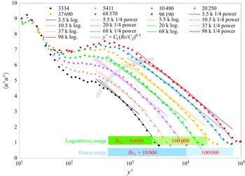


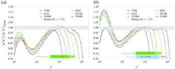


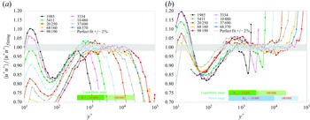


 Open access