2. Prior research

The no-slip boundary condition remains a dependable boundary condition for many macroscopic Newtonian flows. However, when liquids are confined to channels of a width of only a few molecular diameters, the conventional hydrodynamic theories based on the Navier–Stokes equations may fail, and the no-slip boundary condition may no longer be valid (Travis, Todd & Evans Reference Travis, Todd and Evans1997; Travis & Gubbins Reference Travis and Gubbins2000; Zhu & Granick Reference Zhu and Granick2002). Experimental, analytical and numerical studies showed the now well-known slip: that liquids adjacent to a solid move with a finite velocity relative to the solid surface (Lauga et al. Reference Lauga, Brenner and Stone2007; Shu, Teo & Chan Reference Shu, Teo and Chan2018; Wang et al. Reference Wang, Chai, Luo, Liu, Zhang, Wu, Wei and Ma2021). Recently, Hadjiconstantinou (Reference Hadjiconstantinou2024) presented a discussion of the state of the art of the theoretical understanding of slip. Here, we further discuss prior works that are most relevant to our study.

Together with the equations that now bear his name, (Navier Reference Navier1822) derived what became known as the Navier slip condition:

(2.1)\begin{equation} E U + \epsilon\,\frac{{\rm d} U}{{\rm d} z} = 0, \end{equation}

shown here for the tangential component of the liquid velocity $U$ above a flat wall whose normal is in the $z$-direction. Navier delegated constants $E$ and $\epsilon$ as sliding resistances: $\epsilon$ as the sliding resistance between fluid molecules in adjacent layers, the present-day dynamic viscosity, and $E$ as the sliding resistance between the molecules in the vicinal liquid layer and the wall itself, the present-day liquid–solid friction coefficient. The ratio $\epsilon /E$ is the slip length. Navier's presentation was in terms of molecules moving in layers, a point of view that we also use in defining the first liquid layer (FLL) in § 3. In fact, near a wall, the liquid density is layered (Rowley, Nicholson & Parsonage Reference Rowley, Nicholson and Parsonage1976; Abraham Reference Abraham1978). Careful formulations and analyses of the slip boundary condition can be found in Miksis & Davis (Reference Miksis and Davis1994), Brenner & Ganesan (Reference Brenner and Ganesan2000) and Bolaños & Vernescu (Reference Bolaños and Vernescu2017), including over textured and patterned surfaces (Priezjev & Troian Reference Priezjev and Troian2006; Kamrin, Bazant & Stone Reference Kamrin, Bazant and Stone2010; Luchini Reference Luchini2013; Zampogna, Magnaudet & Bottaro Reference Zampogna, Magnaudet and Bottaro2019).

Koplik, Banavar & Willemsen (Reference Koplik, Banavar and Willemsen1989) provided an early yet thorough MD simulation of liquid slip, including examination of Couette and Poiseuille flows, contact line motion, and the trajectories of the individual liquid atoms. Our MD simulation methodology is similar to theirs in that we make use of molecular trajectories to identify the atomic-level mechanisms of liquid slip, as described in § 4.

Models of surface diffusion at the liquid–solid interface have presented the dependence of slip on shear rate, temperature and molecular interaction parameters (Hsu & Patankar Reference Hsu and Patankar2010; Shu et al. Reference Shu, Teo and Chan2018; Wang & Hadjiconstantinou Reference Wang and Hadjiconstantinou2019; Wang et al. Reference Wang, Chai, Luo, Liu, Zhang, Wu, Wei and Ma2021; Shan et al. Reference Shan, Wang, Wang, Zhang and Guo2022). Hadjiconstantinou (Reference Hadjiconstantinou2021) formulated and solved the Fokker–Planck dynamics of a point particle moving in one dimension, driven by shear, slowed by friction with a periodic substrate, and interacting with a thermal background. As shear force is increased, these results reveal slip length at first insensitive to shear, then rapidly increasing to a higher value that once again is invariant to shear. As pointed out by Hadjiconstantinou, these general features of the slip length are consistent with those that were found by other means (Martini et al. Reference Martini, Roxin, Snurr, Wang and Lichter2008b).

Motions more complex than simple diffusion have been anticipated to contribute to the surface transport at the liquid–solid interface. In particular, several types of mechanisms have been described, whereby atoms’ correlated motion with neighbouring atoms has been described as gliding, reptation and dislocation motions (Oura et al. Reference Oura, Lifshits, Saranin, Zotov and Katayama2013). Studies of monolayers range from numerical studies of atoms on atomically structured substrates (Çam, Lichter & Goedde Reference Çam, Lichter and Goedde2021) to micron-sized beads over a laser-generated interference pattern (Reguzzoni et al. Reference Reguzzoni, Ferrario, Zapperi and Righi2010; Brazda et al. Reference Brazda, Silva, Manini, Vanossi, Guerra, Tosatti and Bechinger2018). These studies reveal that even at low levels of forcing, patches of molecules will slip due to the incommensurate alignment between the particles and the surface. In contrast, observations of coordinated motion at the liquid–solid interface under macroscopic flows such as Couette or Poiseuille flow are lacking. It is precisely to seek such coordinated motion that we undertook this investigation.

3. The MD simulations of liquid slip

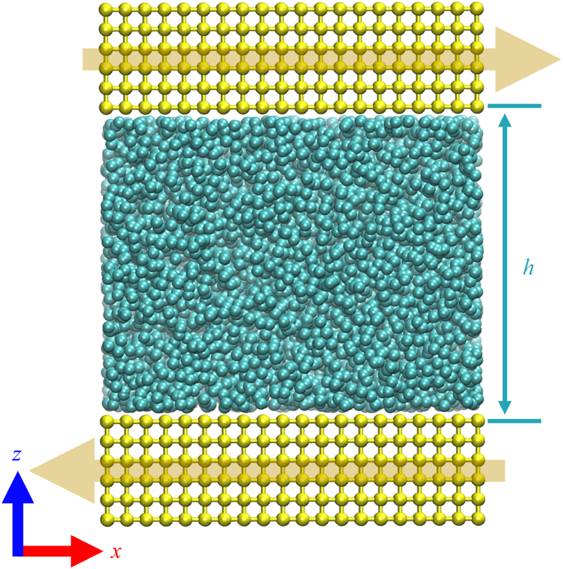
Our non-equilibrium MD simulations are performed using the nanoscale MD (NAMD) programme (Phillips et al. Reference Phillips, Braun, Wang, Gumbart, Tajkhorshid, Villa, Chipot, Skeel, Kale and Schulten2005). We simulate a liquid confined between two thermal solid walls, shown in figure 1. Each wall consists of six $20\times 20$ layers of atoms in the $x$- and $y$-directions. The solid atoms are maintained on a cubic lattice with lattice spacing $\lambda$ by nearest-neighbour linear springs of stiffness 20 N m$^{-1}$. Periodic boundary conditions are implemented along the $x$- and $y$-directions of the square domain, which has dimensions $L_{x} = L_{y} = 20\lambda$. Periodic boundary conditions are also used in the $z$-direction, with the periodic box size chosen to be large enough that the periodic images of the upper and lower walls are always separated by a distance greater than the NAMD non-bonded interaction cutoff distance 1.4 nm. The channel width $h$, equal to the $z$ distance between the mean positions of the innermost solid layers, is 18 liquid molecular diameters.

Figure 1. Snapshot of the Couette flow set-up. Liquid and solid atoms are shown as cyan and yellow spheres, respectively. Solid yellow lines indicate the linear bonds between the nearest-neighbour solid atoms. The direction of motion of each solid wall is shown by a large yellow arrow. The channel width $h$ is the $z$ distance between the mean positions of the innermost solid layers.

The non-bonded interaction potentials are given by

(3.1)\begin{equation} \phi_{ij}(r) = 4\epsilon_{ij} [(\sigma_{ij}/r)^{12} -(\sigma_{ij}/r)^{6}], \end{equation}

where $\phi _{ij}$ indicates the Lennard-Jones interaction strength between atoms of types $i$ and $j$. Indices $i$ and $j$ are chosen to indicate the atomic species, liquid (L) or solid (S). The Lennard-Jones potential provides a simple model of atomic interaction, with only an energy parameter $\epsilon _{ij}$ and a length parameter $\sigma _{ij}$. The energy and length parameters associated with the interactions between the liquid and solid atoms are determined using the Lorentz–Berthelot combining rules (Allen Reference Allen2004):

(3.2a,b)\begin{equation} \sigma_{LS} = \frac{\sigma_{LL} + \sigma_{SS}}{2} \quad \mathrm{and} \quad \epsilon_{LS} = \sqrt{\epsilon_{LL}\epsilon_{SS}}. \end{equation}

Table 1 summarizes the energy and length parameters, and the masses of the liquid and solid atoms. In all simulations, the length parameter for the solid–solid interaction is chosen such that the non-bonded equilibrium spacing of the solid atoms, $r_{0}^{SS}\equiv 2^{1/6}\sigma _{SS}$, is equal to the solid lattice spacing $\lambda$.

Table 1. Lennard-Jones energy $\epsilon _{ij}$ and length $\sigma _{ij}$ parameters associated with the liquid–liquid (LL), solid–solid (SS) and liquid–solid (LS) interactions as well as the masses of liquid and solid atoms. Here, $k_{B}$ is the Boltzmann constant.

In some MD simulations, the solid atoms bounding the liquid flow are fixed in their lattice positions and not given the freedom to fluctuate, constituting a so-called rigid or athermal wall. Martini et al. (Reference Martini, Hsu, Patankar and Lichter2008a) have shown that at high shear rates, slip is more accurately reproduced by allowing the wall atoms to possess their thermal energy and fluctuate, as we do in this study. Furthermore, liquid atomic trajectories are most faithfully simulated when the viscous heat generated by the sheared liquid is allowed to flow to the solid boundaries and, only there, be thermostatted (Bernardi, Todd & Searles Reference Bernardi, Todd and Searles2010; Yong & Zhang Reference Yong and Zhang2013). Therefore, in this study, we thermostat neither the liquid itself nor the adjacent solid layers, but thermostat only the outer solid layers most distant from the liquid.

The simulation protocol consists of three stages. In the first stage, the walls are not yet set into motion while the entire system is coupled to the Langevin thermostat. This first stage allows the liquid atoms to diffuse into random positions. In the second stage, the thermostat is restricted to the two outer solid layers in each wall. During this stage, the top and bottom solid walls accelerate to their target velocities $U_{WALL}$ in the $x$-direction, as shown by the horizontal yellow arrows in figure 1. Target velocities of the top and bottom solid walls are equal in magnitude but opposite in direction. In the third stage, both solid walls move with constant velocity in the $x$-direction. We report only the results obtained during the third stage, in which the average properties of the liquid and solid remain constant.

As discussed in detail below, we carry out two parametric studies. In one, the wall velocity $U_{WALL}$ is systematically varied from 0.2 to 220 m s$^{-1}$. For these studies, we present the slip velocity as a function of shear rate. We calculate the shear rate by finding the slope of a straight-line fit to the liquid velocity profile in $z$-direction near the centre of the channel.

In the second study, we present results where the Lennard-Jones size of the liquid atoms $r_{0}^{LL}\equiv 2^{1/6}\sigma _{LL}$ is kept constant while the lattice spacing $\lambda$ and the solid–solid length parameter $\sigma _{SS}$ are varied, yielding the ratio $r_{0}^{LL}/\lambda$ of the relative size of the liquid atoms to the solid atoms as the control parameter.

For data collection at sampling rate 1 ps, the duration of the third stage is 4–26 ns, depending on the shear rate. For each value of $r_{0}^{LL}/\lambda$, we run four or five simulations with distinct initial positions and velocities for the liquid atoms, while all other simulation parameters remained the same. Sampling at 1 ps would be sufficient if our only objective is to measure the average properties of the system such as temperature, density, slip velocity and slip length. However, it typically takes less than a picosecond for a liquid atom to move from one substrate equilibrium site to the next. Consequently, for our goal to resolve the detailed trajectories of the coordinated motion of individual atoms, femtosecond resolution in atomic positions is needed. In simulations where we gather data on these dynamics, we use sampling rate 10 fs and run the simulations up to 2 ns.

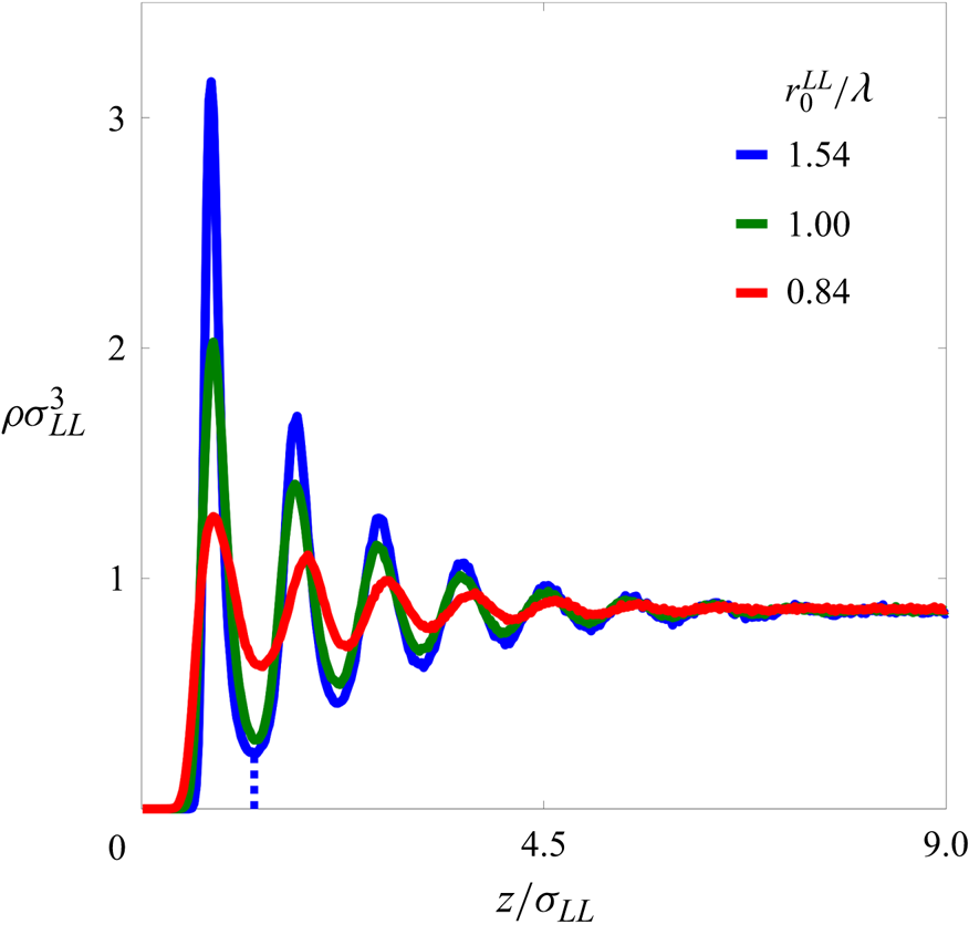
A well-established observation of atomic-level structure is the variation in liquid density near a solid (Rowley et al. Reference Rowley, Nicholson and Parsonage1976; Abraham Reference Abraham1978; Barrat & Bocquet Reference Barrat and Bocquet1999; Morciano et al. Reference Morciano, Fasano, Nold, Braga, Yatsyshin, Sibley, Goddard, Chiavazzo, Asinari and Kalliadasis2017). We too find this layering, and make use of it in our analysis. In particular, we define the FLL as the volume between the mean positions of the innermost solid layer and the first minima of the liquid density profile, as shown in figure 2. Liquid atoms whose positions lie within this volume constitute the FLL. Far enough from the solid walls, the variations disappear and the liquid density becomes constant. The total number of liquid atoms in the channel is chosen such that the liquid density, denoted by $\rho$, has the constant value $\rho =0.87\sigma _{LL}^{-3}$ at the centre of the channel.

Figure 2. The liquid density profiles $\rho \sigma _{LL}^{3}$ as functions of the $z$-position of the liquid atoms $z/\sigma _{LL}$. Here, $z$ is measured relative to the innermost solid layer. Blue, green and red solid lines indicate the liquid density profiles of $r_{0}^{LL}/\lambda = 1.54$, 1.00 and 0.84, respectively. The first minimum defining the upper boundary of the FLL is nearly the same for all densities, and is shown by a dotted blue line for $r_{0}^{LL}/\lambda =1.54$. Far enough from the solid walls, the liquid densities asymptote to a common value $\rho \sigma _{LL}^{3}=0.87$.

Averaging the velocities relative to the moving substrate of all FLL atoms in the $x$-direction over a long enough interval of time yields the slip velocity $U_{FLL}$, shown in figure 3. At lower shear rates, longer simulations are required to resolve the ever-decreasing slip velocity. Simulations at zero shear rate yield zero slip velocity approximately ${\pm }$1 m s$^{-1}$. Thus from zero shear rate to all but the largest shear rates shown in the inset of figure 3, our data are consistent with the proportionality of shear rate and slip velocity. The slopes of the straight-line fit to the data shown in figure 3 yield the Navier slip lengths $(6.47, 0.54, 0.84) \sigma _{LL}$ for the three values of $r_0^{LL}/\lambda$, $(1.54, 1.0, 0.84)$, respectively.

Figure 3. The slip velocity $U_{FLL}$ of the FLL, as a function of the shear rate $\dot {\gamma }$. Blue circles, green triangles and red squares indicate the slip velocities as the substrate wavelength $\lambda$ increases relative to the size $r_0^{LL}$ of the liquid atoms, i.e. $r_{0}^{LL}/\lambda = 1.54$, 1.00 and 0.84, respectively. The dashed lines are linear fits to $U_{FLL}$ for shear rates $\dot {\gamma }<10^{10}\,\mathrm {s}^{-1}$. The slopes of these lines yield Navier slip lengths $(6.47, 0.54, 0.84) \sigma _{LL}$ for blue, green and red, respectively. The inset shows $U_{FLL}$ over a larger range of shear rates.

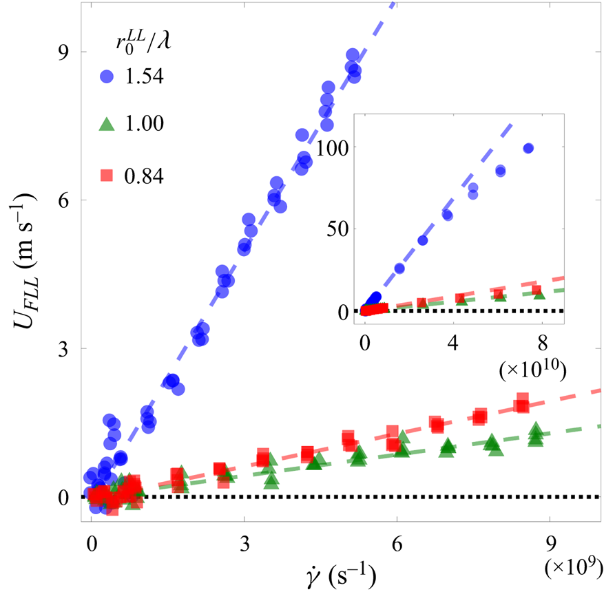
As also shown in the figure, the slip length depends on the lattice spacing of the substrate, with the slip length increasing as the lattice spacing of the substrate decreases. Other researchers have shown the dependence of slip velocity (and slip length) on the geometrical and chemical properties of the substrate (Thompson & Troian Reference Thompson and Troian1997; Barrat & Bocquet Reference Barrat and Bocquet1999). In general, then, we find that slip velocity is not a universal value independent of the spacing of the atoms along the surface, but is dependent on the atomic type and the wavelength of the solid substrate.

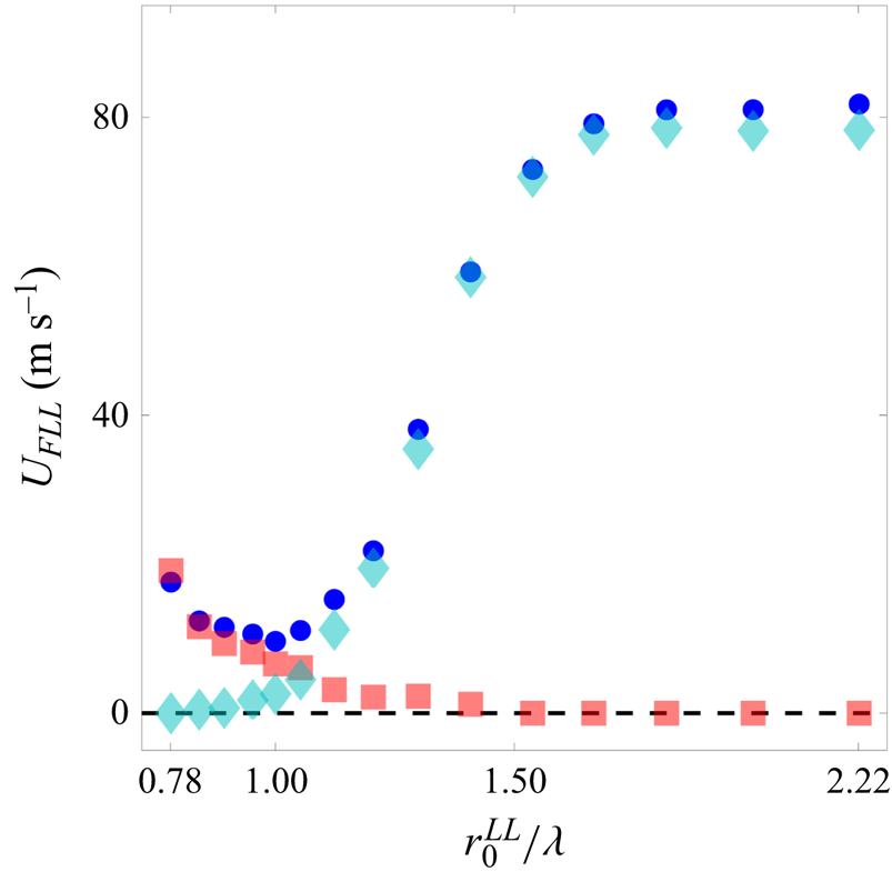
Figure 4 shows the dependence of slip velocity on $r_0^{LL}/\lambda$ for wall speed $U_{WALL}=180$ m s$^{-1}$. Ratios $r_0^{LL}/\lambda <1$ indicate that the substrate lattice spacing is greater than the equilibrium spacing of the liquid atoms. Conversely, ratios $r_0^{LL}/\lambda >1$ indicate that the equilibrium spacing of the solid atoms is smaller than the equilibrium spacing of the liquid atoms. Each data point represents the average of five simulations of duration 6 ns; the error bars represent the standard deviations of each set of five simulations. A minimum in the slip velocity occurs at $r_{0}^{LL}/\lambda =1$, where the substrate wavelength is equal to the equilibrium spacing of the liquid atoms.

Figure 4. A close-up of the slip velocity $U_{FLL}$ of the FLL for $r_{0}^{LL}/\lambda$ near unity. The slip velocity has a minimum at $r_{0}^{LL}/\lambda =1$. Error bars are the standard deviations of five simulations for each $r_{0}^{LL}/\lambda$. Atomic positions and velocities are sampled every 1 ps. Wall speed is $U_{WALL}=180$ m s$^{-1}$. The inset shows $U_{FLL}$ across a wider range, $0.78 \leq r_{0}^{LL}/\lambda \leq 2.22$.

4. Mechanisms of liquid slip

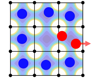
The simple cubic arrangement of the substrate atoms creates a square-symmetric potential energy landscape through which the liquid atoms move, as illustrated in figure 5. On a plane at a small height above the substrate, the largest values of the potential energy are found directly above the substrate atoms. Conversely, the minimum values of the potential energy are located equidistant from four neighbouring solid atoms. We denote these locations, shown as white crosses in the figure, as substrate equilibrium sites. Due to this pattern in the potential energy landscape, the atoms in the FLL are most likely to be found near the substrate equilibrium sites, and they are least likely to be found directly over the locations of the solid atoms. As a result, it is unusual to find more than one liquid atom crowded into the neighbourhood of an equilibrium site. Indeed, a doubly occupied neighbourhood of an equilibrium site is the critical event for localized slip, as we will show.

Figure 5. Potential energy landscape as a function of the $x$- and $y$-positions of a liquid atom at a fixed height above the substrate. The strength of the potential energy is colour-coded as dark blue for low and bright yellow for high potential energy locations. White cross markers indicate the substrate equilibrium sites. Horizontal and vertical white dashed lines indicate low-energy corridors connecting neighbouring equilibrium sites. Filled black circles indicate the lattice positions of the solid substrate atoms. Solid vertical and horizontal black lines indicate the boundaries of substrate cells, as defined in the text. A patch of only 9 cells of 400 is shown here.

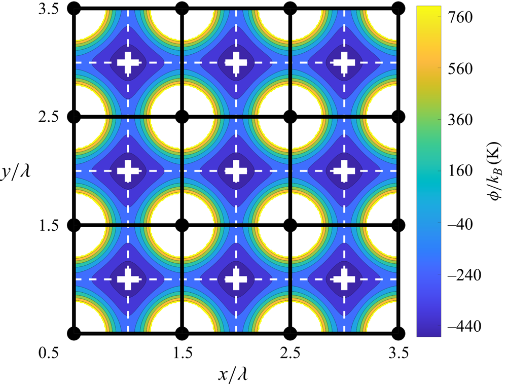
Using the pattern shown in figure 5, we divide the FLL into 400 cuboidal substrate cells, each centred over a substrate equilibrium site. The base of each cell is bounded by four substrate atoms (the black circles in figure 5) and the (black) lines connecting them. The height of the cells is equal to the height of the FLL. In figure 5, we show a top view of a patch of 9 neighbouring cells (out of 400 total for our $20\times 20$ periodic lattice) superimposed on the substrate potential energy landscape.

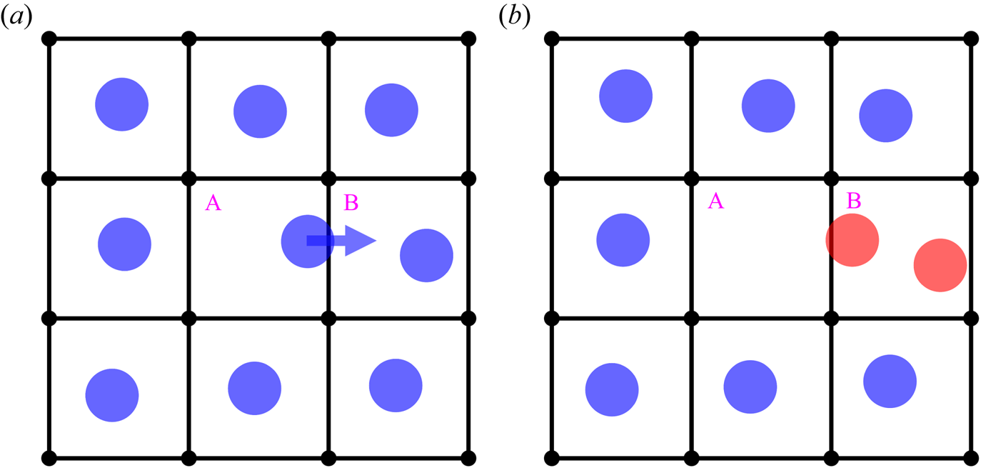
Using the data from simulations sampled every 10 fs, we label and identify all the liquid atoms in the FLL, and track the position of each uniquely labelled atom in time, paying particular attention to the cell that each liquid atom occupies. This allows us to follow each atom in the FLL as it moves between substrate cells. Figure 6 shows a schematic view of a typical event as an atom in the FLL hops from one cell to the next. In figure 6(a), each cell is occupied by a single liquid atom, which is a common configuration of atomic positions in the FLL. However, a liquid atom can spontaneously move from its current cell into an already-occupied cell, creating a doubly occupied cell. Figure 6 shows an example in which a liquid atom moves from the cell labelled A to the cell labelled B in the time between Figures 6(a,b), creating doubly occupied cell B, and leaving behind vacant cell A.

Figure 6. Schematic representation of liquid atoms (blue circles) on a small square grid of cells at two consecutive instants of time, shown in (a,b), respectively. Due to the $x$-motion of a liquid atom, shown by the horizontal blue arrow from cell A to cell B, cell A becomes vacant, and cell B becomes doubly occupied. In (a), each cell is occupied by a single liquid atom. In (b), cell A is not occupied by any liquid atom and is a vacant cell, and cell B, occupied by two liquid atoms (each coloured red), is designated as a doubly occupied cell. (The diameter of the liquid atoms is chosen for clarity and does not represent their characteristic size.)

After an atom moves into an already-occupied cell, the original occupant of the now doubly occupied cell can become dislodged and move forward, so the double occupancy moves onwards into the adjacent cell. This process can repeat itself, as shown schematically in figure 7. As the doubly occupied cell propagates, atoms advance by one cell forwards. Therefore, the mean motion of the entire layer can be produced by the few atoms moving quickly and sequentially from one doubly occupied cell to the next, in a coordinated fashion.

Figure 7. Schematic representation of a doubly occupied cell moving in the $x$-direction. A horizontal strip of seven neighbouring cells in the $x$-direction is shown, sampled at four consecutive instants, from (a) to (d). As the doubly occupied cell moves, atoms advance by one cell in the $x$-direction, and the pair of atoms in the doubly occupied cell (coloured red) evolves sequentially. Horizontal red arrows indicate the atoms that advance into the next cell. Also shown by the horizontal blue arrow, in the time between (c) and (d), is the motion of a liquid atom from a singly occupied cell into a vacant cell, resulting in the vacant cell moving one cell to the left.

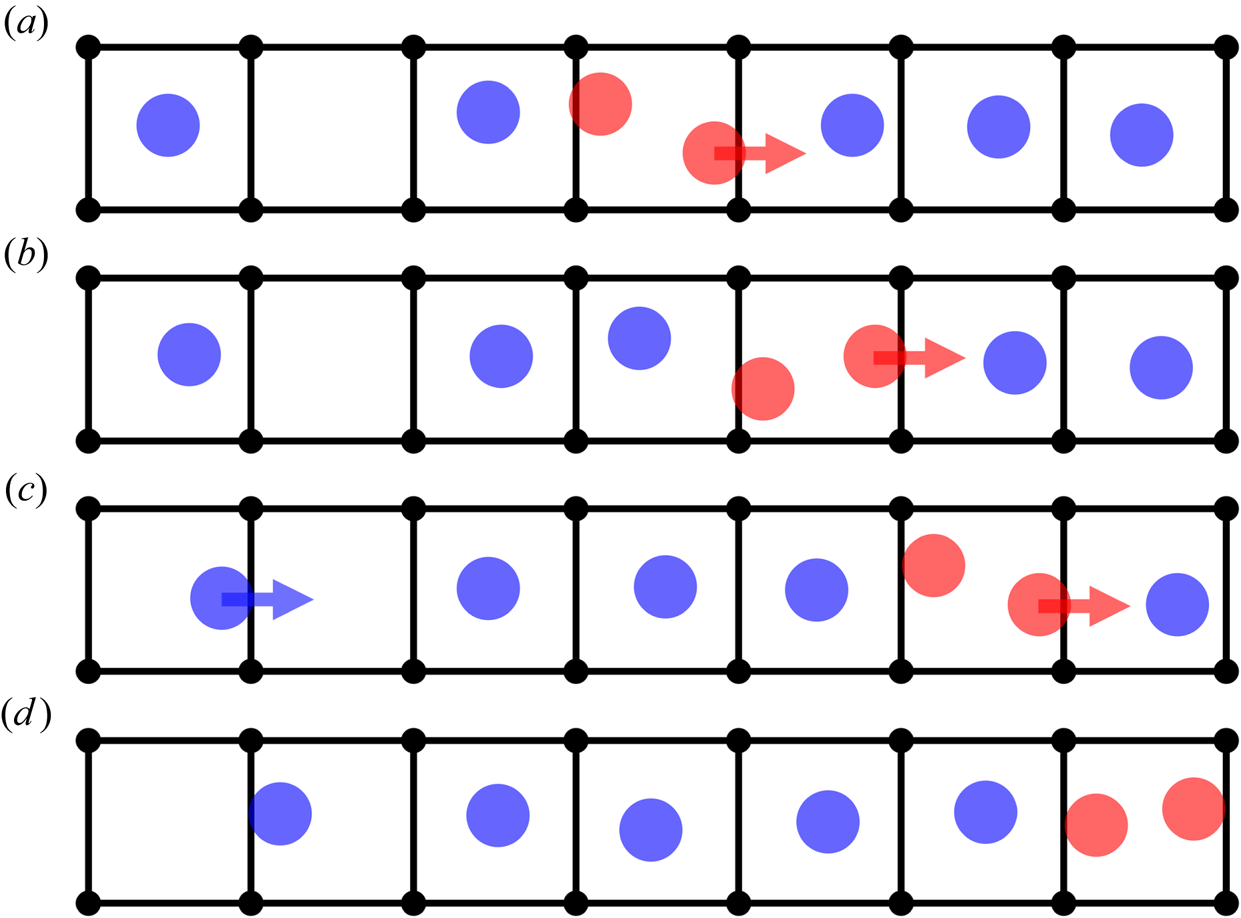
The motion of a liquid atom into a vacant (unoccupied) cell is quite different from the motion of an atom into an already-occupied cell. When a liquid atom moves into a vacant cell, nearby liquid atoms are nearly unaffected. Therefore, such motion represents an uncoordinated, independent atomic motion over the substrate, which is the typical description of surface diffusion as a mechanism of slip.

We identify and distinguish every instance of an atomic hop either into an already-occupied cell or into a vacant cell. We track the motion in both the $x$- and $y$-directions. However, as there is no net motion in the transverse $y$-direction, we restrict our analysis here to the $x$-direction only.

Using the data from simulations sampled at 10 fs, we separately calculate the net liquid displacement in the $x$-direction due to (i) atomic motion involving doubly occupied cells, and (ii) atomic motion into vacant cells. When divided by the duration of the simulation and the time-averaged number of atoms in the FLL, these displacements provide the fractional contributions to slip due to atomic motion into doubly occupied or vacant cells.

In figure 8, we show the slip velocity of the FLL over the range $0.78 \leq r_0^{LL}/\lambda \leq 2.22$ for wall speed $U_{WALL}=180\,\mathrm {m}\,\mathrm {s}^{-1}$. For each value of $r_0^{LL}/\lambda$, we run a single simulation with sampling rate 10 fs and simulation duration 2 ns. The blue circles show the slip velocity for the layer as calculated directly from the atomic velocities. (This is the same range of data as shown in figure 4.) The red squares show the slip velocity due only to motion involving doubly occupied cells. The cyan diamonds show only the slip due to atomic motion into vacant cells. Taken together, the sum of these two contributions accounts for the totality of the slip. Liquid slip due to doubly occupied cells becomes increasingly predominant as $r_{0}^{LL}/\lambda$ decreases. The cross-over value of $r_{0}^{LL}/\lambda$ at which the contributions to slip are equally divided between doubly occupied cells and atoms hopping into vacant cells occurs near $r_{0}^{LL}/\lambda \simeq 1$. Slip is overwhelmingly due to doubly-occupied cells for $r_{0}^{LL}/\lambda < 1$, and continues to contribute significantly to slip even for values of $r_{0}^{LL}/\lambda$ above unity.

Figure 8. The slip velocity $U_{FLL}$ of the FLL, as a function of $r_{0}^{LL}/\lambda$, at the wall speed $U_{WALL}=180$ m s$^{-1}$. Blue circles indicate the slip velocity as determined by the direct measurement of the atomic velocities. Red squares indicate the slip velocity due to the mass propagation involving doubly occupied cells alone. Cyan diamonds indicate the slip velocity due to the mass propagation by atoms hopping into vacant cells. Atomic positions and velocities are sampled every $10$ fs.

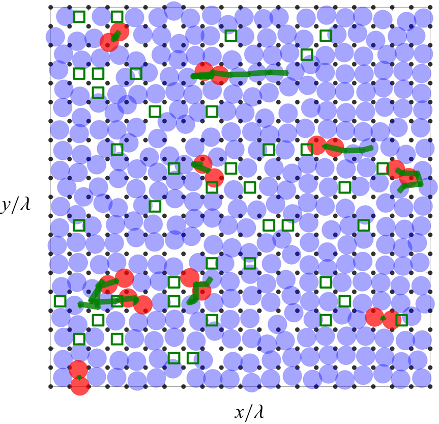
To provide a sense of the role played by vacant and doubly occupied cells in the generation of slip, figure 9 shows an annotated view of the entire FLL obtained from the simulation with $r_{0}^{LL}/\lambda =1$ at wall speed $U_{WALL}=20$ m s$^{-1}$ and sampling rate 10 fs. Approximately 5 % of the liquid atoms are in a doubly occupied cell, while approximately 95 % of the atoms merely fluctuate around their equilibrium sites. Also shown are the trajectories of doubly occupied cells as they were tracked moving over several cells; for these parameter values, the lifetime of the motion involving a doubly occupied cell is typically a few picoseconds.

Figure 9. Portrait of the FLL constructed from the MD data. The blue translucent circles indicate the instantaneous positions of the liquid atoms. Liquid atoms in doubly occupied cells are coloured red. The thick green lines indicate the trajectories over time of doubly occupied cells. The open green squares indicate vacant cells. The black dots indicate the lattice positions of the solid substrate atoms. The mean slip direction is to the right. Here, the wall speed is $U_{WALL}=20$ m s$^{-1}$, $r_{0}^{LL}/\lambda =1$, and the atomic positions are sampled every 10 fs.

To highlight the sequential nature of the atomic motion involving doubly occupied cells, we show in figure 10 the $x$-positions of six neighbouring liquid atoms as a function of time as the atoms hop in the $x$-direction between doubly-occupied sites. The atomic positions shown are obtained from the same simulation that is used to generate figure 9. The actual atomic trajectories are shown in figure 10(a); a schematic representation of the motion is shown in figure 10(b) for clarity.

Figure 10. Atomic trajectories illustrating coordinated atomic motion into or out of doubly occupied cells. (a) Excerpt from our MD data, simplified in (b) to highlight the advance of each liquid atom 1–5 from one equilibrium site to the downstream site. Each atom 1–5 is advanced one substrate lattice spacing in the $x$-direction by the passage of the doubly occupied cell, instantaneously located at the thickened red portion of the atomic trajectories. The thin vertical orange lines mark the first and final times of the occurrence of the doubly occupied cell. The $x$-boundaries between cells are marked by dashed grey lines. Note that the liquid atoms tend to remain near the substrate minima located halfway between adjacent dashed lines. Magenta portions of the atomic trajectories mark when the atom has drifted out of the FLL. Here, the wall speed is $U_{WALL}=20$ m s$^{-1}$, $r_{0}^{LL}/\lambda =1$, and the atomic positions are sampled at every 10 fs.

In this example, atom 1 starts in cell A and hops to cell B near $t=5$ ps, creating a doubly occupied cell, which is indicated by highlighting the trajectories for atoms 1 and 2 in red. The interaction of atoms 1 and 2 results in atom 2 hopping from cell B to cell C (already occupied by atom 3). In this manner, the doubly occupied site propagates from cell B to cell F. The sequence terminates when atom 6 moves into the unoccupied cell G at the top of the diagram. The sequence of doubly occupied cells exists during the time interval between the two vertical orange lines, for approximately 0.5 ps. During this period, the doubly occupied cell translates by five substrate wavelengths, and five atoms propagate by one lattice spacing forwards.

5. Frenkel–Kontorova model of slip

The two atoms in doubly occupied cells are part of a larger number of atoms whose motion is correlated. When properly visualized, this group of atoms is seen to take on a shape that is characteristic of nonlinear waves in the sine-Gordon equation and Frenkel–Kontorova (FK) model (Braun & Kivshar Reference Braun and Kivshar1998).

We define an offset for each atom near the doubly occupied cell,

(5.1)\begin{equation} \textrm{[offset of atom $k$]}=\frac{x_k(t)-k\lambda}{\lambda}, \end{equation}

where $x_k(t)$ is the $x$-coordinate of atom $k$, and $k\lambda$ is the position of the atom's initial substrate equilibrium site.

Figure 11 shows the offsets of the atoms in the neighbourhood of a propagating doubly occupied cell. Downstream of the doubly occupied cell, atoms gradually move away from their equilibrium sites as they are swept into the doubly occupied cell. As the doubly occupied cell propagates onwards, upstream atoms relax into new equilibrium sites after being transported one cell forward. These profiles, such as shown in figure 11, thereby refer to the distribution of atomic offsets relative to the atoms’ initial equilibrium positions. So offset 0 shows that atom $k$ has not moved away from its initial site, while offset 1 indicates that the atom has been transported forwards by the distance of one substrate cell. Thus the doubly occupied cell marks a larger propagating structure of displaced atoms that we call a kink.

Figure 11. Time-averaged kink profiles derived from atomic positions in the FLL of the MD simulations. Data points of blue triangles, green circles and red squares are the mean values of atomic offsets from MD simulations with $r_{0}^{LL}/\lambda$ for 1.08, 1.00 and 0.87, respectively. The wave profiles are well described by (5.2), shown as solid curves, with steepnesses $A=0.27$ (blue triangles), $A=0.44$ (green circles) and $A=0.85$ (red squares). The location of the doubly occupied cell that marks the centre of the propagating kink is shown by the diamond at the top of the figure.

The profiles seen in figure 11 can be fitted to the sigmoid function

(5.2)\begin{equation} \textrm{[offset of atom $k$]}=\frac{2}{\rm \pi}\tan^{{-}1} \{\exp[{-}A(k-k_0)]\}, \end{equation}

where the parameters $A$ and $k_0$ describe the steepness of the profile and the location of its centre, respectively. This function is the discrete version of the soliton solution to the sine-Gordon equation, which is the continuum limit of the standard FK model (Braun & Kivshar Reference Braun and Kivshar1998).

For each of the three curves shown in figure 11, the data points are the time-averaged atomic positions over the lifetime of one kink. All frames are centred by aligning the location of the doubly occupied cell. The curves are then generated by fitting the averaged atomic positions to the sigmoidal (5.2) to find $A$ and $k_0$ for each profile.

To understand the shape and behaviour of the kinks observed in the MD simulations, we model the FLL using a modified version of the one-dimensional FK model. The FK model describes $N$ particles along the $x$-axis at positions $x_k(t)$, $k=1, 2, \ldots, N$, that are interacting through a linear spring force with their neighbouring particles, and are also interacting with a sinusoidal force that arises from the periodic potential of the adjacent substrate (Braun & Kivshar Reference Braun and Kivshar1998). If the spacing between the particles is precisely equal to the wavelength of the potential, then the particles achieve their lowest energy state with each particle at the periodically located potential minima. When an additional particle is present, such that there are one too few minima to host each of the particles, the FK model predicts that the spacing between particles is no longer uniform. While most particles remain periodically placed close to substrate potential minima, a few particles within a narrow spatial interval are crowded together. Thus the FK model can be used to understand the profiles shown in figure 11.

For our application, the particles of the FK model are the liquid atoms, and the potential is due to the substrate of solid atoms. Prior work showed that the FK model provides a description of the dependence of slip on shear rate (Lichter, Roxin & Mandre Reference Lichter, Roxin and Mandre2004; Martini et al. Reference Martini, Roxin, Snurr, Wang and Lichter2008b). Furthermore, predictions of the FK model agree with the observations that slip is bounded in the limit of large shear rates over thermalized solid substrates (Martini et al. Reference Martini, Hsu, Patankar and Lichter2008a). Though these studies gave evidence that the FK model could describe certain aspects of mean slip, there was little comparison with the observations at the molecular scale. This was due to the lack of data on molecular trajectories and the absence of a conceptual framework that permitted the localized propagating structures to be identified and extracted from the noisy MD data. These deficiencies have been overcome in the present work through the recognition of the doubly occupied cell.

To more realistically model the interactions between neighbouring atoms in a liquid, we replace the linear nearest-neighbour coupling of the classical FK equation with a nearest-neighbour force arising from the 12-6 Lennard-Jones potential. In addition, the liquid atoms are forced into motion by a shear force of the form $\eta _{LL}(V-\dot {x}_k)$, where $V$ is the constant velocity of the liquid layer above, and $\eta _{LL}$ is the friction coefficient between the adjacent liquid layers. As the liquid atoms move with speed $\dot {x}_k$ over the substrate, they are also subject to a frictional force proportional to their speed $\eta _{LS}\dot {x}$, where $\eta _{LS}$ is the liquid–solid friction coefficient.

With these modifications, the FK model becomes

(5.3)\begin{align} \ddot{x}_k &={-}\sin{(x_k)} \nonumber\\ &\quad + g\left[\left(\frac{\sigma}{x_{k+1}-x_k}\right)^7- 2\left(\frac{\sigma}{x_{k+1}-x_k}\right)^{13} -\left(\frac{\sigma}{x_k-x_{k-1}}\right)^7+ 2\left(\frac{\sigma}{x_k-x_{k-1}}\right)^{13}\right] \nonumber\\ &\quad +\eta_{LL}(V-\dot{x}_k) - \eta_{LS}\dot{x}_k, \end{align}

where

(5.4a,b)\begin{equation} g=\frac{12\epsilon_{LL}\lambda}{{\rm \pi} \sigma_{LL} \phi_{0}} \quad \mathrm{and} \quad \sigma = \frac{2{\rm \pi}\sigma_{LL}}{\lambda}, \end{equation}

and where the particle positions and time have been non-dimensionalized in the usual way (Braun & Kivshar Reference Braun and Kivshar1998). The non-dimensional parameter $g$ signifies the strength of the liquid–liquid interaction relative to that of the liquid–substrate interaction. The ratio of the characteristic size of the liquid atoms relative to the lattice spacing, $\sigma$, plays an important role in setting the ground state and the dynamics of the solutions to the FK equation (Aubry Reference Aubry1983; Braun & Kivshar Reference Braun and Kivshar1998).

The dimensionless parameters defined in (5.4a,b) depend on the dimensional liquid–liquid Lennard-Jones energy $\epsilon _{LL}$, the length parameter of the liquid–liquid interaction $\sigma _{LL}$, the substrate wavelength $\lambda$, and the dimensional amplitude of the sinusoidal substrate potential energy $\phi _{0}$. While the first three can be taken directly from the input parameters for the MD simulations, the substrate potential amplitude used in the FK model must be estimated from the MD interaction potential between all the substrate atoms and an atom in the FLL. We do this by calculating the potential energy above two $(x,y)$-locations in the MD simulations: (i) a substrate equilibrium site, yielding $\phi _{eqb}(z)$; and (ii) halfway between two neighbouring equilibrium sites, yielding $\phi _{jump}(z)$. Atoms in the FLL of the MD simulations are expected to tend towards heights at which the potentials are at a minimum. We therefore take the substrate potential amplitude for the modified FK model to be one-half of the difference between the minimum values of $\phi _{eqb}(z)$ and $\phi _{jump}(z)$, yielding

(5.5)\begin{equation} \phi_{0} = \frac{\min{[\phi_{jump}(z)]} - \min{[\phi_{eqb}(z)]}}{2}. \end{equation}

This results in a substrate potential amplitude for the modified FK model $\phi _{0}/k_{B} \simeq 35.5(1.1-r_{0}^{LL}/\lambda ) + 66$ K.

We use the modified FK model to describe the dynamics of the atoms near a doubly occupied substrate cell. As in our MD simulations, we use periodic boundary conditions in the modified FK model, with periodic domain length $(N-1)\lambda$, where $N$ is the number of particles. This assures that there is an extra particle in the FK chain relative to the number of substrate potential minima. Figure 12(a) shows numerical solutions of the FK equations (5.3) at multiple instants of time. We call these nonlinear wave solutions to the FK model ‘FK kinks’. FK kinks propagate at a constant speed with an invariant profile. The FK kink profiles are closely approximated by the sine-Gordon soliton solution (dotted curves) from the sigmoid function (5.2). The profile can be characterized succinctly by its steepness parameter $A$, which indicates the narrowness of the FK kink profiles, three of which are shown in figure 12(b).

Figure 12. Numerical results from the FK model. (a) The propagation of a single FK kink through 52 contiguous atoms is shown at intervals of 0.7 ps. The two atoms instantaneously inside a doubly occupied cell are highlighted in red, and the locations of their centres of mass are shown by diamonds at the top of the figure. The dotted lines at the initial and final frames are the nearly identical sine-Gordon soliton profiles, fitted with $A=0.27$ for $r_{0}^{LL}/\lambda =1$. (b) Time-averaged FK kink profiles for three different values of $r_{0}^{LL}/\lambda$, showing the steepening profile as $r_{0}^{LL}/\lambda$ decreases: blue triangles for $r_{0}^{LL}/\lambda = 1.08$, $A=0.17$; green circles for $r_{0}^{LL}/\lambda = 1.00$, $A=0.27$; red squares for $r_{0}^{LL}/\lambda = 0.87$, $A=0.56$. Data points are from numerical solutions to the FK model, and correspondingly coloured curves are best fits from the sigmoid function (5.2).

To compare the wave properties of MD kinks to FK kinks, we compare their velocities and narrowness. Figure 13(a) shows the velocity of the kinks, $v_{k}$, in both the MD and FK simulations as a function of $r_{0}^{LL}/\lambda$. We calculate kink velocities in the MD simulations by dividing the kink displacements in the $x$-direction by their lifetimes. It is observed that the kink velocities in MD simulations increase as $r_{0}^{LL}/\lambda$ increases. This trend is also observed in our FK simulations. The agreement between the kink velocities from MD and FK simulations gets better as $r_{0}^{LL}/\lambda$ decreases, where we can sample a larger number of propagating kinks, which is signified by smaller error bars. Figure 13(b) shows the steepness parameter $A$ of the kinks of both the MD and FK simulations as a function of $r_{0}^{LL}/\lambda$. Kinks get narrower as $r_{0}^{LL}/\lambda$ decreases.

Figure 13. Results from the MD simulations compared with those from the FK model. (a) The kink velocity $v_{k}$ as a function of $r_{0}^{LL}/\lambda$. Filled red circles indicate the average MD kink velocities. The thick green line indicates the velocities of the FK kinks obtained from the FK simulations. (b) The steepness parameter $A$ of the kinks as a function of $r_{0}^{LL}/\lambda$. The MD data (filled red circles) were averaged over all kinks that propagated at least four substrate wavelengths. Error bars are the standard deviations of all those kinks for each $r_{0}^{LL}/\lambda$. For the green line of the FK model, we set $V=1$, and use values $\epsilon _{LL}/k_{B}=188\,\mathrm {K}$, $\sigma _{LL}=(2{\rm \pi} )2^{-1/6}$, $\phi _{0}/{k}_{B}\simeq 70\,\mathrm {K}$, identical to those of the MD simulation. The friction factors were chosen to comply with the high shear rate limit of the FK equation, $\eta _{LL}/\eta _{LS}={O}(1)$; see Appendix A.

When compared with the predictions of the modified FK model, both the profile shape, as measured by $A$, and the velocity of the kinks seen in the MD simulations, show similar trends and comparable values as a function of $r_{0}^{LL}/\lambda$. In assessing the agreement between the two sets of data, the extreme simplicity of the FK model should be recalled. In the FK model, particles move in only one dimension and the system is closed. This is to be contrasted with the three-dimensional motion of atoms in the MD simulations in which atoms continually move into and out of the FLL. In the FK model, the particles experience the substrate through a potential with a simple sinusoidal variation. This is to be compared with a substrate potential due to the summation of the Lennard-Jones potentials of the solid substrate atoms. Not only is the Lennard-Jones potential itself more complex than that of the sinusoidal FK potential, but the potential experienced by the liquid atoms further varies as they fluctuate along their $y$ and $z$ degrees of freedom. Additionally, the MD simulation incorporates finite temperature and heat fluxes that are absent in the FK model. Given these differences, the rather striking degree of similarity delivered by the FK model can be taken as evidence of the importance of geometry, particularly the ratio $r_{0}^{LL}/\lambda$, in governing the dynamics.

Finally, we note that unlike the coordinated kink motion described above, atomic motion into an unoccupied cell does not create the same extended atomic profile as seen in figure 12 and is not described by an FK kink. This difference is due to the asymmetry of the Lennard-Jones potential in the modified FK model (5.3). The Lennard-Jones potential produces the nonlinear wave profile of a kink because its nonlinear repulsive force is huge for liquid atoms brought close together. In contrast, it produces no such profile in the neighbourhood of a vacant cell, because it is only slightly attractive for liquid atoms separated across a vacant cell.