





Introduction
Site-specific weed management (SSWM) is a method wherein weed control treatments are adjusted within a crop field to match the variation in location, density, and composition of the weed population (Wiles Reference Wiles2009). Weed spatial distribution within a crop can be mapped using remote sensing technologies, such as aerial or satellite imagery, or through proximal sensing techniques, which involve in-field sensors mounted on machines like harvesters, tractors, or robots (López-Granados Reference López-Granados2010). Weed maps play a crucial role in SSWM strategies, enabling practices such as targeted application with postemergence herbicides (Allmendinger et al. Reference Allmendinger, Spaeth, Saile, Peteinatos and Gerhards2024; Hunter et al. Reference Hunter, Gannon, Richardson, Yelverton and Leon2020), adjustment of herbicide applications according to weed species composition (López-Granados Reference López-Granados2010), and variable-rate application of preemergence herbicides to target persistent weed patches (Koller and Lanini Reference Koller and Lanini2005).
Recent advancements in machine vision, particularly through deep learning algorithms, have facilitated the development of more efficient weed mapping systems. Convolutional neural networks (CNNs) are deep learning architectures that can identify and learn spatial hierarchies of features, such as edges, textures, and shapes, from image data. CNNs have been utilized in both pixel-level and object-level approaches for detecting and identifying weeds. Pixel-level approaches, such as semantic segmentation, classify each pixel in an image into a specific class, such as weeds, crop, or soil. Semantic segmentation has been widely applied for weed mapping, particularly using imagery collected with unmanned aerial systems (UAS) (Huang et al. Reference Huang, Lan, Yang, Zhang, Wen and Deng2020; Liu et al. Reference Liu, Jin, Han, He, Wang, Chen, Kong and Yu2024; Lottes et al. Reference Lottes, Behley, Milioto and Stachniss2018; Sa et al. Reference Sa, Popović, Khanna, Chen, Lottes, Liebisch, Nieto, Stachniss, Walter and Siegwart2018). This approach enables the generation of weed cover maps, representing the spatial extent of weed canopy cover across the field (Zou et al. Reference Zou, Chen, Zhang, Zhou and Zhang2021). While semantic weed mapping has proven valuable for creating prescription maps for targeted application with postemergence herbicides (Huang et al. Reference Huang, Deng, Lan, Yang, Deng, Wen, Zhang and Zhang2018), it is unable to separate individual weeds and therefore cannot be used to predict the number of weeds present within an image (Coleman et al. Reference Coleman, Bender, Hu, Sharpe, Schumann, Wang, Bagavathiannan, Boyd and Walsh2022). Additionally, it typically classifies all weeds as a single category, rather than distinguishing species or groups (e.g., grasses and sedges), limiting effective analysis of weed distribution as spatial and temporal patterns vary by species (Blank et al. Reference Blank, Rozenberg and Gafni2023; Cardina et al. Reference Cardina, Johnson and Sparrow1997).
Object-level approaches identify individual objects within images, facilitating tasks like weed counting. Bounding-box detection algorithms, for instance, generate pixel coordinates for boxes around each object, providing spatial information for every object within an image. You Only Look Once (YOLO) is a family of architectures comprising state-of-the-art object detection algorithms that have proven highly effective for weed detection (Barnhart et al. Reference Barnhart, Lancaster, Goodin, Spotanski and Dille2022; Dang et al. Reference Dang, Chen, Lu and Li2023; Pérez-Porras et al. Reference Pérez-Porras, Torres-Sánchez, López-Granados and Mesas-Carrascosa2023; Sharpe et al. Reference Sharpe, Schumann, Yu and Boyd2020; Wu et al. Reference Wu, Wang, Zhao and Qian2023). YOLO streamlines the detection process by integrating feature extraction and bounding-box prediction into a single network pass (Redmon et al. Reference Redmon, Divvala, Girshick and Farhadi2016), enabling fast and accurate identification and localization of weeds in agricultural settings. YOLO models have been applied to UAS imagery for weed detection, achieving high detection accuracy and enabling the generation of weed maps (Khan et al. Reference Khan, Tufail, Khan, Khan and Anwar2021; Luo et al. Reference Luo, Chen, Wang, Fu, Mi, Wang, Li, Shi and Su2025; Pei et al. Reference Pei, Sun, Huang, Zhang, Sheng and Zhang2022; Zhang et al. Reference Zhang, Wang, Hu, Liu, Chen and Su2020). However, achieving the fine detail necessary to distinguish individual weeds often requires flying at very low altitudes, which in turn increases flight duration and operational complexity. In contrast, ground-based platforms with cameras offer significantly higher resolution, enabling the detection of individual weeds with YOLO models, and have been used in tasks such as real-time targeted herbicide application (Buzanini et al. Reference Buzanini, Schumann and Boyd2024, Reference Buzanini, Furlanetto, Schumann and Boyd2025; Partel et al. Reference Partel, Charan Kakarla and Ampatzidis2019). Coupling object detection algorithms with GPS data can enable the estimation of the real-world coordinates of detected weeds within georeferenced images. This process can enable the creation of weed population maps at the individual-weed level and could be integrated into tractor-mounted camera systems to monitor weeds during routine field operations such as spraying and fertilizer application.
Despite the widespread application of object detection models for weed recognition, this approach still faces limitations in detecting weeds across varying growth stages and densities, which can affect the accuracy and reliability of weed population maps generated from detection outputs. A significant challenge is weed occlusion, where overlapping vegetation obscures key morphological features, reducing detection accuracy (Gao et al. Reference Gao, French, Pound, He, Pridmore and Pieters2020). This problem becomes more pronounced in high-density weed infestations and with larger plants, where extensive overlap complicates the identification of individual weed instances. Barnhart et al. (Reference Barnhart, Lancaster, Goodin, Spotanski and Dille2022) found a linear decline in YOLOv5 detection performance with increasing Palmer amaranth (Amaranthus palmeri S. Watson) density up to approximately 30 plants m−2, maintaining F1 scores above 0.8 at the highest density across all heights evaluated. While this demonstrates that model performance is sensitive to weed density, it remains unclear whether this relationship would persist under more severe infestations or dense clusters that can occur in field conditions. Moreover, object detection models for weed recognition are typically trained on images with low to moderate plant densities, where individual weeds are clearly visible and can be accurately annotated. However, object detection models are used in fields with heterogeneous weed distributions, where areas of high density and dense vegetation may occur, conditions typically absent from training data due to the difficulty of labeling such scenarios. Therefore, understanding how detection performance degrades with increasing weed density and canopy coverage is essential for defining the practical limits of these models for weed mapping.
The present study focuses on evaluating the impact of increasing weed density on an object detection model performance, using purple nutsedge (Cyperus rotundus L.) as a model species. Cyperus rotundus is one of the most troublesome weeds worldwide, affecting multiple crops in more than 90 countries in tropical and subtropical regions (Bendixen and Nandihalli Reference Bendixen and Nandihalli1987). It features shiny, dark-green, three-ranked leaves emerging in an unfolded triangular fascicle from basal bulbs, forming a basal rosette as they gradually unfurl outward (Wills Reference Wills1987; Wills and Briscoe Reference Wills and Briscoe1970). The rachis is erect, solid, and triangular in cross section, supporting terminal inflorescences with reddish-brown spikelets (Wills Reference Wills1987). Cyperus rotundus spreads primarily through a complex underground system of tubers and basal bulbs connected by rhizomes, with limited seed dispersal (Calderon and Odero Reference Calderon and Odero2021; Horak et al. Reference Horak, Holt and Ellstrand1987; Stoller and Sweet Reference Stoller and Sweet1987). This vegetative propagation often results in clusters with high density of C. rotundus causing the occlusion of morphological features due to overlapping plants within the cluster. Given the increased feature occlusion under higher density and larger size of C. rotundus, we hypothesize that these factors significantly affect model performance. Therefore, this study aimed to (1) evaluate the impact of increased density and canopy coverage of C. rotundus on a detection model, including density scenarios that extend beyond the range represented in the training dataset; (2) quantify limitations in density for achieving reliable weed counts within images; and (3) assess the overall robustness of a C. rotundus detection model.
Materials and Methods
Experimental Setup and Design
Greenhouse experiments were conducted at the University of Florida, Gulf Coast Research and Education Center (GCREC) in Wimauma, FL (27.7601°N, 82.2286°W) from April to December 2023 to develop a density test dataset for evaluating the performance of a YOLOv8 model in detecting C. rotundus at increasing plant density. Tubers of C. rotundus were collected from naturally occurring populations in strawberry [Fragaria × ananassa (Weston) Duchesne ex Rosier ssp. ananassa] and cantaloupe (Cucumis melo L.) fields at the GCREC research farm. Tubers of C. rotundus were planted on growing trays filled with a commercial potting medium (Peatlite Mix, Speedling, Ruskin, FL, USA) on April 21, 2023, and November 8, 2023, for the first and second experimental iterations, respectively, in a greenhouse maintained at a maximum temperature of 27 C. Cyperus rotundus plants with three unfolded leaves were transplanted into 46 by 33 cm trays filled with commercial potting medium (Peatlite Mix, Speedling) on April 28, 2023, and November 19, 2023, for the first and second experimental iterations, respectively.
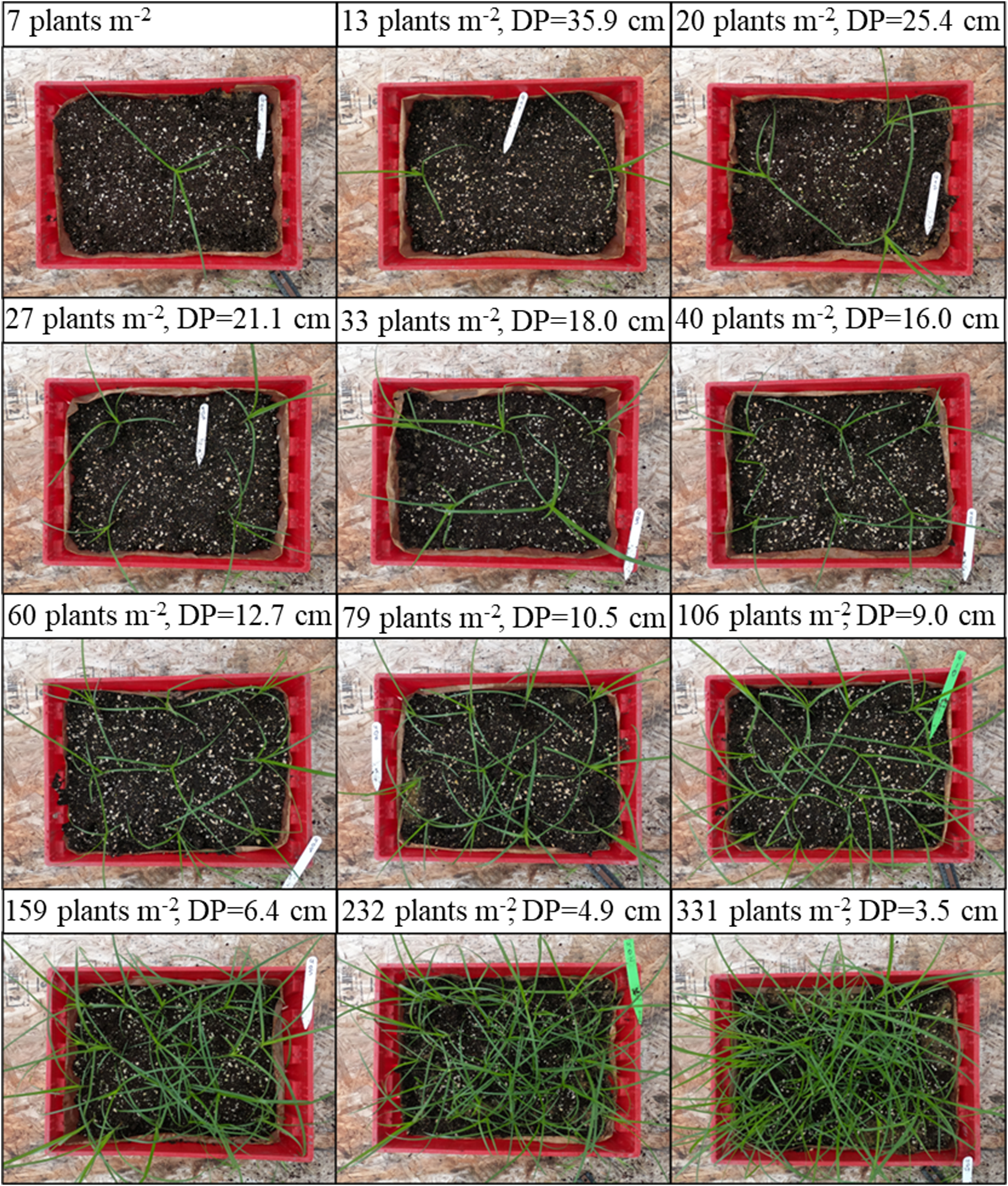
The experimental design was a randomized complete block design with four replications, repeated twice. A total of 12 densities were assessed, consisting of an increasing number of C. rotundus plants per tray at 7, 13, 20, 27, 33, 40, 60, 79, 106, 159, 232, and 331 plants m−2, (Figure 1). This setup was designed to ensure that each increase in density leads to a proportional reduction in the distance between plants. Due to the prolific tuber production and subsequent emergence of new C. rotundus plants, manual hand-pulling was performed daily to maintain the predetermined plant densities. Trays were watered as needed.
Cyperus rotundus density levels and corresponding distance between plants (DP).

Preparation of Density Test Dataset
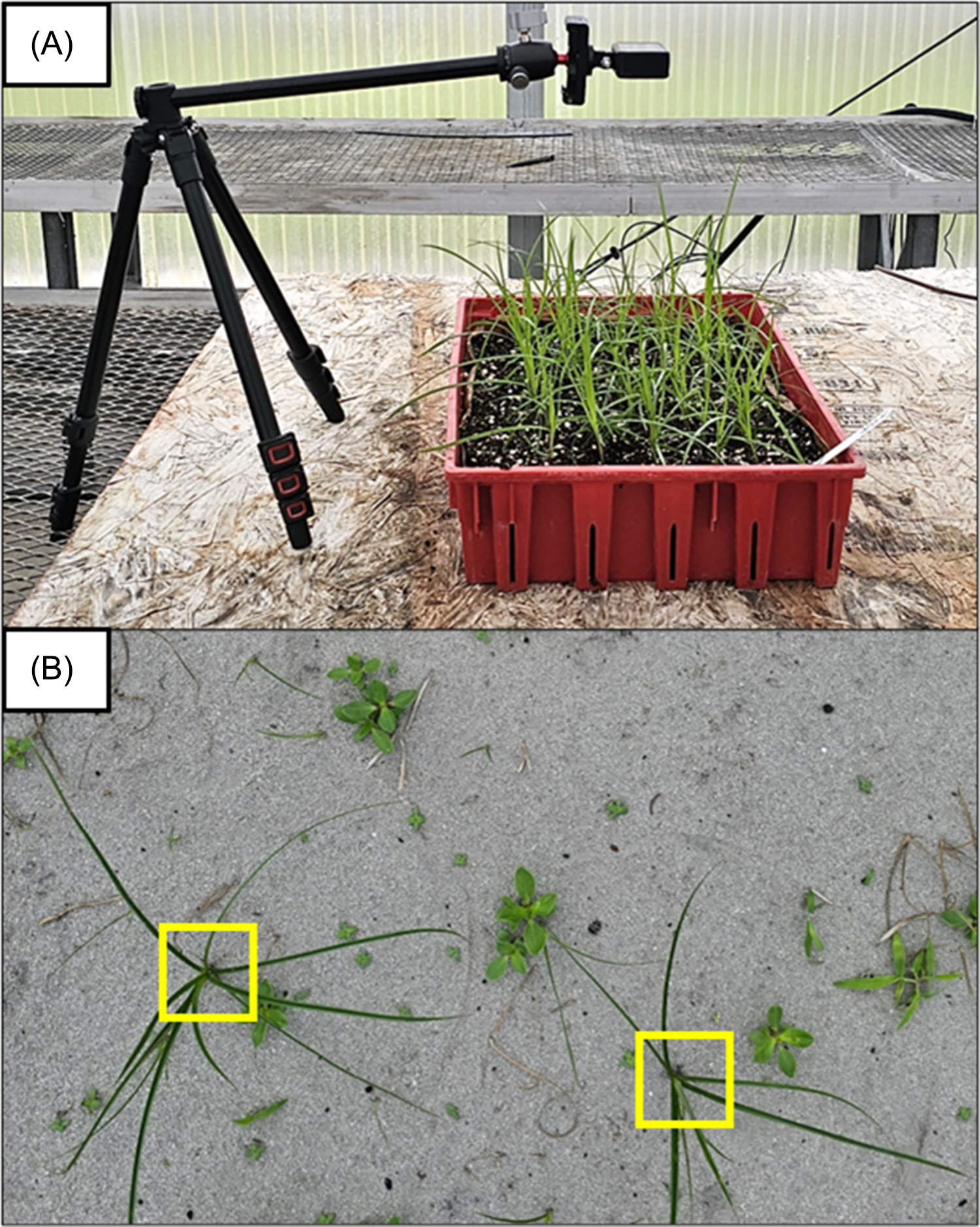
The density test dataset was generated by photographing all density treatments at transplant and at 3, 6, 10, and 17 d after transplanting (DATr) during both experimental iterations. Photographs of individual trays were captured using a GoPro Hero 8 camera (GoPro, San Mateo, CA, USA) with a resolution of 2,704 by 1,520 pixels. The camera was placed on a tripod pointing directly toward the ground at a height of 36 cm from the soil surface within the tray (Figure 2A). A total of 240 images were collected for each experimental iteration, resulting in a total density test dataset of 480 images. Importantly, images from the density test dataset were not manually annotated because the extensive overlap and occlusion of plant structures in high-density and dense-canopy conditions made accurate labeling unreliable. As a result, subsequent evaluations using this dataset were conducted through visual inspection of the detection outputs.
(A) Camera setting for image collection for the density test dataset. (B) Cyperus rotundus annotation with bounding boxes, focusing on basal rosette.

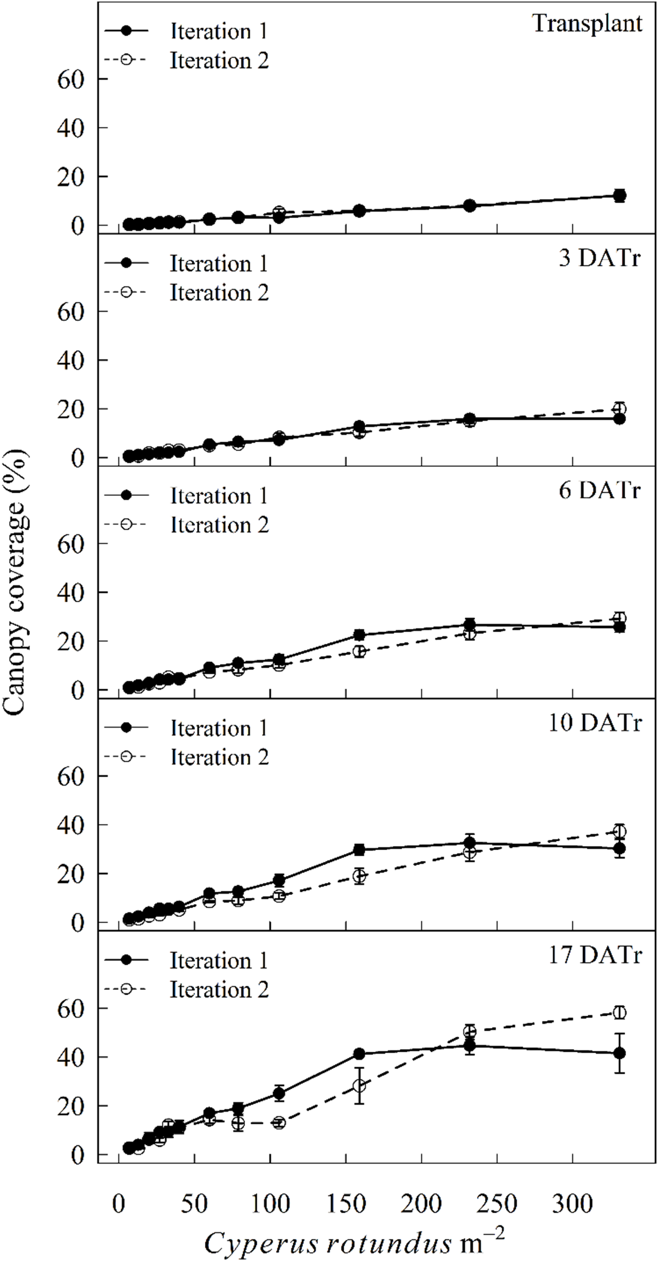
Canopy coverage for each tray was quantified to confirm consistent growth patterns between experimental iterations. A custom Python script was used to analyze the digital images by segmenting vegetation pixels and comparing them with a standardized background image captured under identical conditions but without vegetation. This process produced a percentage-based estimate of canopy coverage for each image at every evaluation time point, allowing verification that both experimental iterations exhibited comparable growth and canopy development across all densities (Figure 3).
Canopy coverage of Cyperus rotundus across densities at transplant and at 3, 6, 10, and 17 d after transplanting (DATr) for each iteration.

Preparation of Training and Validation Dataset
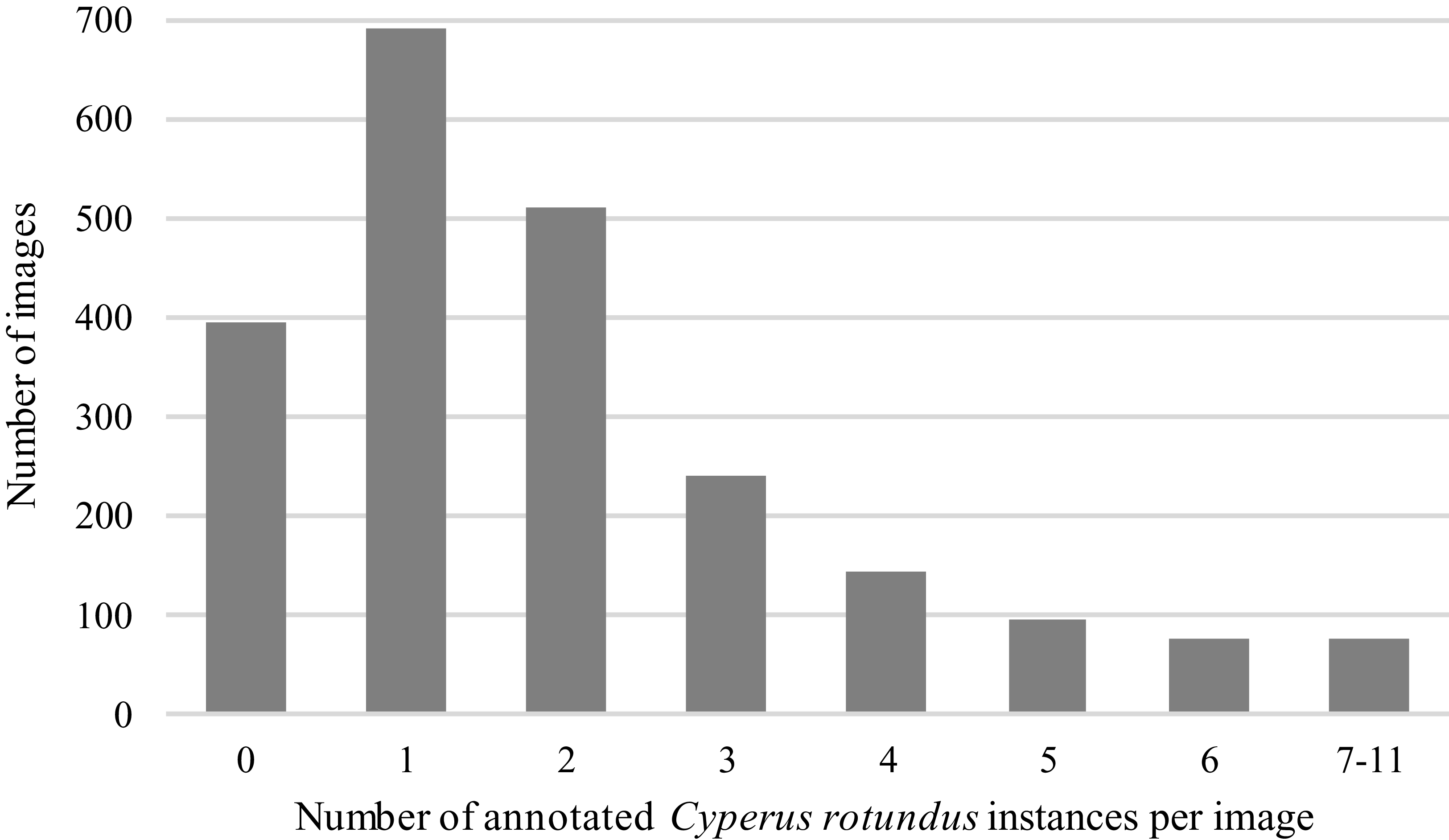
A dataset of 2,221 images, independent from the density test dataset, was used for model training and validation. Images were acquired using a GoPro Hero 8 and an Akaso V50 Pro (Akaso Tech, Shenzhen, China) at the GCREC and in commercial strawberry fields in Dover, FL. The dataset included images captured under both field and greenhouse conditions (Table 1). The field images included scenes from tomato (Solanum lycopersicum L.) and strawberry fields with polyethylene mulch–covered beds at early crop stages, showing C. rotundus growing on the beds, in sandy row middles, and in fallow areas with sandy soils. Greenhouse images were incorporated to align with the visual domain of the density test dataset and minimize potential effects of background variation. These images were obtained from a different C. rotundus population than those used in the density test dataset but were captured under identical conditions, including trays, potting medium, and camera setup. All annotated C. rotundus plants across both field and greenhouse images were in the vegetative growth stage, from when the first three leaves unfolded to advanced canopy development, with no flowering stage present. All images with the presence of C. rotundus across both field and greenhouse conditions contained between 1 and 11 C. rotundus plants (Figure 4). In the greenhouse subset, specifically, the number of plants per tray ranged from 1 to 9, corresponding to 7 to 60 plants m−2. This upper limit was established because scenes with higher densities and dense canopies, which caused partial or complete occlusion of target structures, made consistent labeling difficult, thereby maintaining a comparable representation of plant densities across different levels of canopy development.
Summary of the image subsets used for YOLOv8 model training and validation for Cyperus rotundus detection.

Distribution of annotated Cyperus rotundus instances per image in the training and validation dataset (n = 2,221).

The images were manually annotated using the YOLO-Label software (https://github.com/developer0hye/Yolo_Label). The labeling approach consisted of drawing bounding boxes around the basal leaf rosette, where the leaves originate and are most concentrated, focusing on capturing the characteristic triangular stem and leaf arrangement of C. rotundus while minimizing background inclusion (Figure 2B). This approach resulted in limited variation in object sizes across annotated instances, as bounding boxes were consistently centered on the basal region rather than scaled to overall plant size; thus, object dimensions did not vary in proportion to canopy expansion. Of the 2,221 images, 1,826 contained annotated C. rotundus instances, while the remaining 395 images did not contain any C. rotundus plants and therefore had no class labels assigned. These images were added as unlabeled background samples to reduce false positives during detection and enhance robustness. These included trays with potting medium but no C. rotundus plants, collected under the same conditions as the density test dataset, as well as field scenes with soil, mulch, and unannotated vegetation (Table 1). The dataset of 2,221 images was randomly split into 90% for training and 10% for validation to monitor performance and guide model selection. Data augmentation was performed before training using Roboflow (Roboflow, Des Moines, IA, USA) to increase dataset diversity and improve model generalization. Augmentations included random horizontal and vertical flips, bright adjustments between −20% and +20%, and blur up to 10 px. A total of 6,017 augmented images were generated and added to the dataset for model training.
Model Training
The training dataset was used to train a single-class YOLOv8 extra-large model (Ultralytics, Los Angeles, CA, USA) using the Ultralytics 8.1.46 package on the HiPerGator high-performance computing cluster. The system operated on Linux with software libraries including CUDA 12.1 (NVIDIA Corp.), Python 3.11.4 (Python Software Foundation), Open CV 4.8.0 (Open Source Vision Foundation), PyTorch 2.1.0+cu121 (Pytorch Foundation), and the Jupyter Notebook (Project Juypter) as an interactive computing environment. The model was trained with an auto batch size, an initial learning rate of 0.01, a final learning rate of 0.001, and an image resolution of 640 by 640 pixels. Training consisted of 250 epochs with a momentum of 0.9, and early stopping was applied with a patience of 50 epochs to prevent overfitting. All default augmentation parameters were disabled, except for mosaic augmentation, which remained active with its default settings. All other parameters remained at their default values.
Detection Model Evaluation and Statistical Analysis
The validation dataset, which is 10% of the annotated training data, was used during training to monitor performance and select the best model. The best model was selected based on the epoch in which it achieved the highest mean average precision (mAP) across intersection over union (IoU) thresholds ranging from 0.5 to 0.95 (mAP@[0.5:0.95]) on the validation dataset. IoU measures the overlap between the predicted and ground-truth bounding boxes, calculated as the area of intersection divided by the area of their union. After training, the independent density test dataset was used to evaluate detection performance across increasing C. rotundus densities and canopy coverage. The confidence threshold for the density test dataset, referring to the probability that a prediction must exceed to be considered positive, was selected based on the F1 score curve of the validation dataset.
The detection outputs of each image in the density test dataset were manually inspected to record the counts of true positives, false positives, and false negatives in each of the 480 images. True positives represent instances where the model correctly identified C. rotundus, false positives indicate instances where the model incorrectly identified as C. rotundus, and false positives indicate instances where the model incorrectly identified C. rotundus where it was not present in the images. These values were aggregated across all 480 images to calculate precision, recall, and F1 score, providing an estimate of model robustness across the full range of densities and canopy cover. Precision, recall, and F1 score were calculated using the following equations:
 $${\rm{Precision}} = \;{{{\rm{True}}\;{\rm{positives}}} \over {{\rm{True}}\;{\rm{positives}} + {\rm{False}}\;{\rm{positives}}}}$$
 $${\rm{Recall}} = \;{{{\rm{True}}\;{\rm{positives}}} \over {{\rm{True}}\;{\rm{positives}} + {\rm{False}}\;{\rm{negatives}}}}$$
 $$\!\!\!\!\!\!\!\!\!\!\!\! {\rm{F}}1\;{\rm{score}} = \;2\; \times \;{{{\rm{Precision}}\; \times {\rm{Recall}}} \over {{\rm{Precision}} + {\rm{Recall}}}}$$
Precision measures the accuracy of the positive predictions made by the model, indicating the proportion of correct positive identifications out of all positive identifications made. Recall measures the ability of the model to identify all actual positive instances, indicating the proportion of true positives out of all actual instances. The F1 score is the harmonic mean of precision and recall, providing a single metric that balances the trade-off between precision and recall.
To assess the impact of density on model performance at each data-collection time point, precision, recall, and F1 score were calculated for every image and averaged within each density treatment at each time point. These metrics were analyzed for interactions between experimental iterations with a linear mixed-effect model using the lme4 package in R v. 4.4.1 (R Core Team 2022). Nonlinear regression analysis was conducted using the Regression Wizard in SigmaPlot 15 software (Systat Software, San Jose, CA, USA). A four-parameter logistic sigmoidal model was fit to assess the F1 score as a function of increasing density of C. rotundus at each data-collection time point, defined by the equation:
 $${\rm{\widehat {\it y}}} = {y_0} + {\rm{\;}}{a \over {1 + {\rm{\;}}{e^{ - \left( {{{x - {x_0}} \over b}} \right)}}}}$$
where ${\rm{\widehat {\it y}}}$
represents F1 score, and x represents C. rotundus density. The parameter y 0 is the minimum asymptote, a represents the range of the F1 score, x 0 represents the inflection point, and b is the slope of the curve at the inflection point.
${\rm{\widehat {\it y}}}$
represents F1 score, and x represents C. rotundus density. The parameter y 0 is the minimum asymptote, a represents the range of the F1 score, x 0 represents the inflection point, and b is the slope of the curve at the inflection point.
Results and Discussion
Model Performance on Validation Dataset
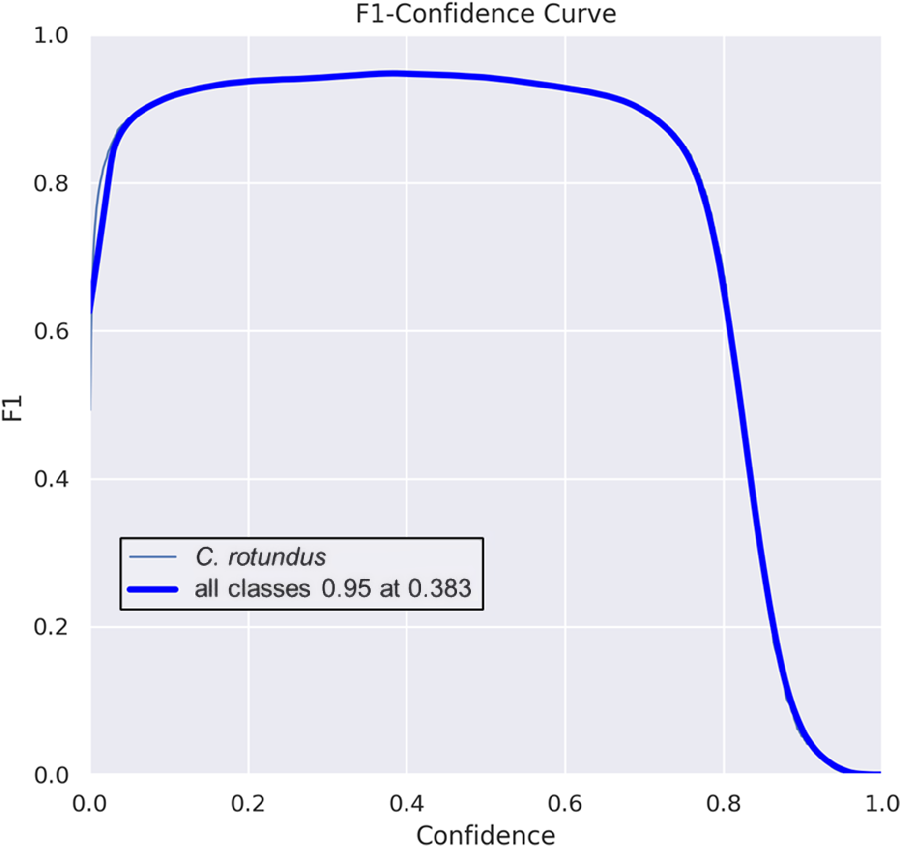
The selected model achieved a mAP of 0.58, computed across IoU thresholds from 0.5 to 0.95 (mAP@[0.5:0.95]), and a precision and recall of 0.96 and 0.93, respectively, on the validation dataset. Precision and recall are highly sensitive to the confidence level used for predictions, as the choice of confidence threshold significantly impacts the number of false positives and false negatives (Wenkel et al. Reference Wenkel, Alhazmi, Liiv, Alrshoud and Simon2021). A low confidence threshold could result in fewer false negatives at the expense of an increased number of false positives. Conversely, a high confidence threshold would result in fewer false positives but more false negatives. When mapping weeds, it is likely that a low confidence threshold would overestimate the weed population, while a high confidence threshold would underestimate it, impacting the accuracy of the estimated weed population. Therefore, it is crucial to determine a confidence threshold that ensures the best prediction accuracy and balance between precision and recall. In the selected model, the F1 score, the harmonic mean of precision and recall, remained high across a broad range of confidence levels, dropping sharply when confidence exceeded 0.75 (Figure 5). The F1 score was maximized at 0.95 with a confidence level of 0.383; therefore, this value was used as the confidence threshold for making predictions on all images within the density test dataset.
F1 score vs. confidence level curve for Cyperus rotundus classification.

Model Robustness
Evaluation of the trained model on the complete density test dataset, which included images with C. rotundus densities ranging from 7 to 331 plants m−2 and covers all data-collection time points, resulted in a precision of 0.97, a recall of 0.49, and an F1 score of 0.65. The lower performance on the density test dataset can be attributed to the differences between the validation and density test datasets. The validation dataset, derived from a subset of the training data, primarily includes images with minimal overlapping vegetation and limited variability in basal rosette development. In contrast, the density test dataset was designed to represent more complex scenarios with greater canopy overlap and occlusion that are rarely included in training datasets due to the difficulty of accurate labeling at high densities. In agricultural settings, weeds are typically present in patches within the field (Dieleman et al. Reference Dieleman, Mortensen and Martin1999), meaning cameras may capture anything from sparse weed areas to dense clusters with significant occlusion. The evaluation on the density test dataset provided a more comprehensive assessment of detection performance across a wide range of weed densities and canopy overlap likely to occur under field conditions.
Density and Canopy Coverage Impact on Model Performance
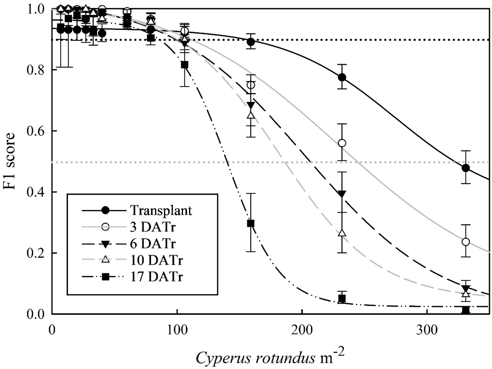
No significant interactions with experimental iteration were observed for any of the model evaluation metrics (P > 0.05); therefore, both experimental iterations were combined for analysis. There were sigmoidal relationships between F1 score and C. rotundus density for all data-collection time points (R2 = 0.988 to 0.998) (Table 2). The F1 score remained high at low C. rotundus densities and declined as density increased at each time point (Figure 6). Except for at transplant and 3 DATr, when minimum F1 scores were 0.43 and 0.24, respectively, all other time points showed a decline in F1 score to nearly 0 at the highest C. rotundus density. Similarly, a study on the detection of A. palmeri using a YOLOv5 model showed decreased algorithm performance at higher densities (Barnhart et al. Reference Barnhart, Lancaster, Goodin, Spotanski and Dille2022). In high-density environments, the presence of overlapping structures, such as leaves, leads to occluded or partially occluded plants. This poses a significant challenge for the model, which is designed to detect within the basal leaf rosette of nutsedge plants. The complete or partial occlusion of features in these conditions increases the likelihood of false negatives. Previous research has highlighted similar challenges. Dyrmann et al. (Reference Dyrmann, Jørgensen and Midtiby2017) found that the performance of weed detection models declines significantly when weeds experience severe overlap. Gao et al. (Reference Gao, French, Pound, He, Pridmore and Pieters2020) also noted the increased difficulty in accurately detecting weeds under conditions of heavy overlap. More recently, Wu et al. (Reference Wu, Wang, Zhao and Qian2023) reported that in high-density weed scenarios, the decreased performance of detection models is attributed to a reduced ability to extract features, leading to inaccurate predictions of the target. These findings underscore the complexity of accurately detecting weeds in dense, overlapping conditions. Although a decrease in F1 score due to missed individuals in high-density areas is a limitation for weed mapping, it does not necessarily translate to reduced effectiveness in real-time targeted herbicide applications, as the herbicide may be deposited on neighboring weeds even if they were not individually identified.
Estimated parameters for the four-parameter logistic sigmoid model characterizing the impact of Cyperus rotundus density on the F1 score of a YOLOv8x detection model across combined density test dataset experimental iterationsa.

a  , where ${\rm{\hat y}}$
represents F1 score, and x represents C. rotundus density. The parameter y 0 is the minimum asymptote, a represents the range of the F1 score, x 0 represents the inflection point, and b is the slope of the curve at the inflection point. SEs are in parentheses.
${\rm{\hat y}}$
represents F1 score, and x represents C. rotundus density. The parameter y 0 is the minimum asymptote, a represents the range of the F1 score, x 0 represents the inflection point, and b is the slope of the curve at the inflection point. SEs are in parentheses.
b DATr, days after transplanting.
c RMSE, root mean-square error.
Influence of Cyperus rotundus density on detection model F1 score at each time point, combined for both experimental iterations. The dotted horizontal lines indicate F1 score thresholds of the optimal model performance (black, 0.9 F1 score) and marginal model performance (gray, 0.5 F1 score).

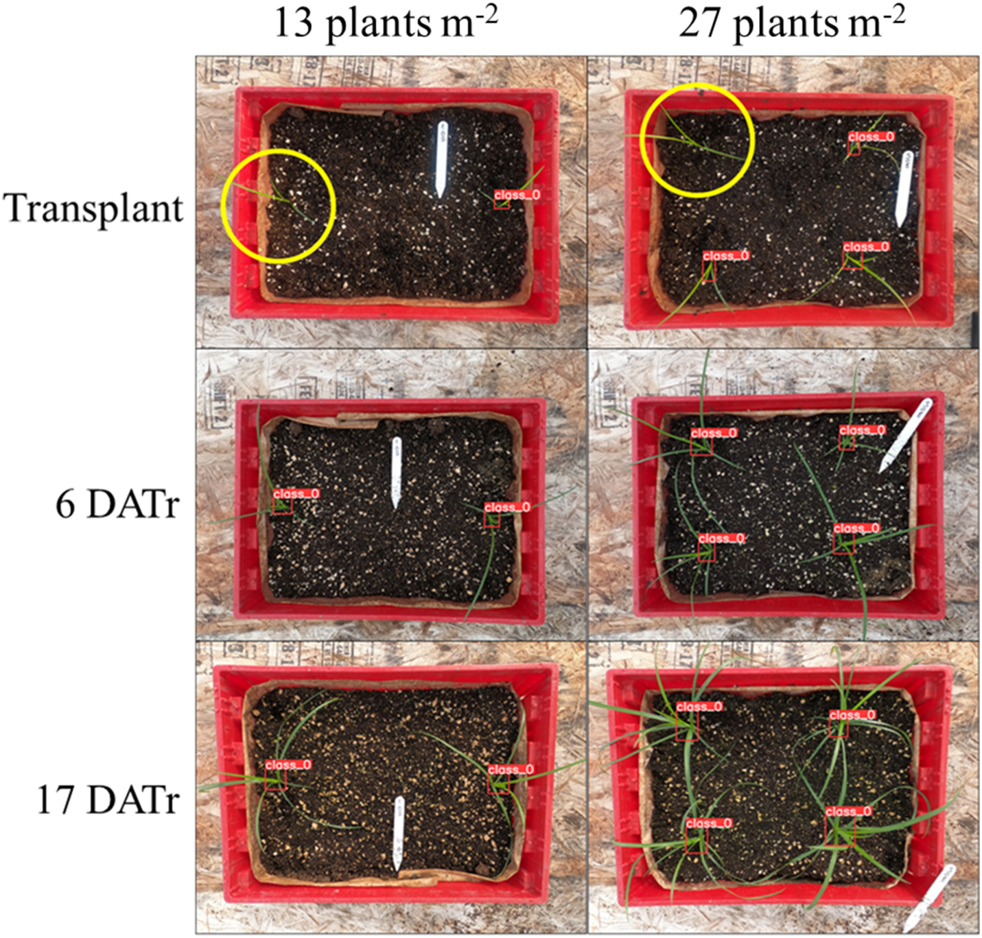
At low densities, where overlapping of plant parts is minimized, an F1 score above 0.90 was achieved at all time points (Figure 6). However, detection performance showed greater variation at transplant, with a higher number of false negatives compared to later time points, as shown in Figure 7. This inconsistency had a great impact on the F1 score at low densities, as missing a single plant had a larger effect on accuracy due to the smaller number of plants in the image. These results suggest potential limitations in reliability and detection accuracy during early development, when the basal rosette is less distinct and bounding boxes include a larger proportion of background relative to plant tissue. Furlanetto et al. (Reference Furlanetto, Schumann and Boyd2024) reported that a YOLOv4 model, with a limited number of small plants in its training dataset, had difficulties identifying early stages of poison ivy [Toxicodendron radicans (L.) Kuntze] due to the absence of distinctive characteristics typical of developed plants. Conversely, Barnhart et al. (Reference Barnhart, Lancaster, Goodin, Spotanski and Dille2022) reported better predictions for smaller A. palmeri, potentially attributed to a greater number of instances of smaller plants in the training dataset. In our study, we did not explicitly ensure balanced representation of C. rotundus plants with different degrees of basal rosette development, which may have contributed to variable performance in detecting plants at early development. Other factors, such as image resolution and model selection, may influence the detection of early-developing C. rotundus plants. These are characterized by narrow leaves and smaller fascicles. As the plants mature and produce additional leaves, the fascicles become denser, forming a more prominent basal leaf rosette and a more distinct triangular arrangement. Small objects, which occupy fewer pixels and contain less available information compared to larger objects, often exhibit significantly lower detection performance (Wei et al. Reference Wei, Cheng, He and Zhu2024). Coleman et al. (Reference Coleman, Kutugata, Walsh and Bagavathiannan2024) suggested that smaller model architectures combined with higher image resolutions are more effective for detecting seedlings of A. palmeri. Additionally, enhancements to YOLOv8 models, such as incorporating small-target detection layers and optimizing feature extraction mechanisms, have been shown to significantly improve performance for small-weed detection (Guo et al. Reference Guo, Ling, Tan, Wang, Wu and Yang2023). For weed mapping and geospatial analysis, recognizing both early and later stages of weed growth is critical for understanding weed population dynamics within fields and for designing site-specific weed management strategies for subsequent years. Thus, future research should focus on evaluating different YOLO versions, implementing model enhancements, and developing balanced training datasets to improve the detection of C. rotundus plants with less prominent basal rosettes without compromising the accuracy of detecting more-developed plants.
Comparison of the model performance in detecting Cyperus rotundus at different densities at transplant and 6 and 17 d after transplanting (DATr). Red bounding boxes indicate predictions made by the model. The yellow circles highlight plants where the model resulted in false negatives.

Thresholds for Optimal and Marginal Model Performance
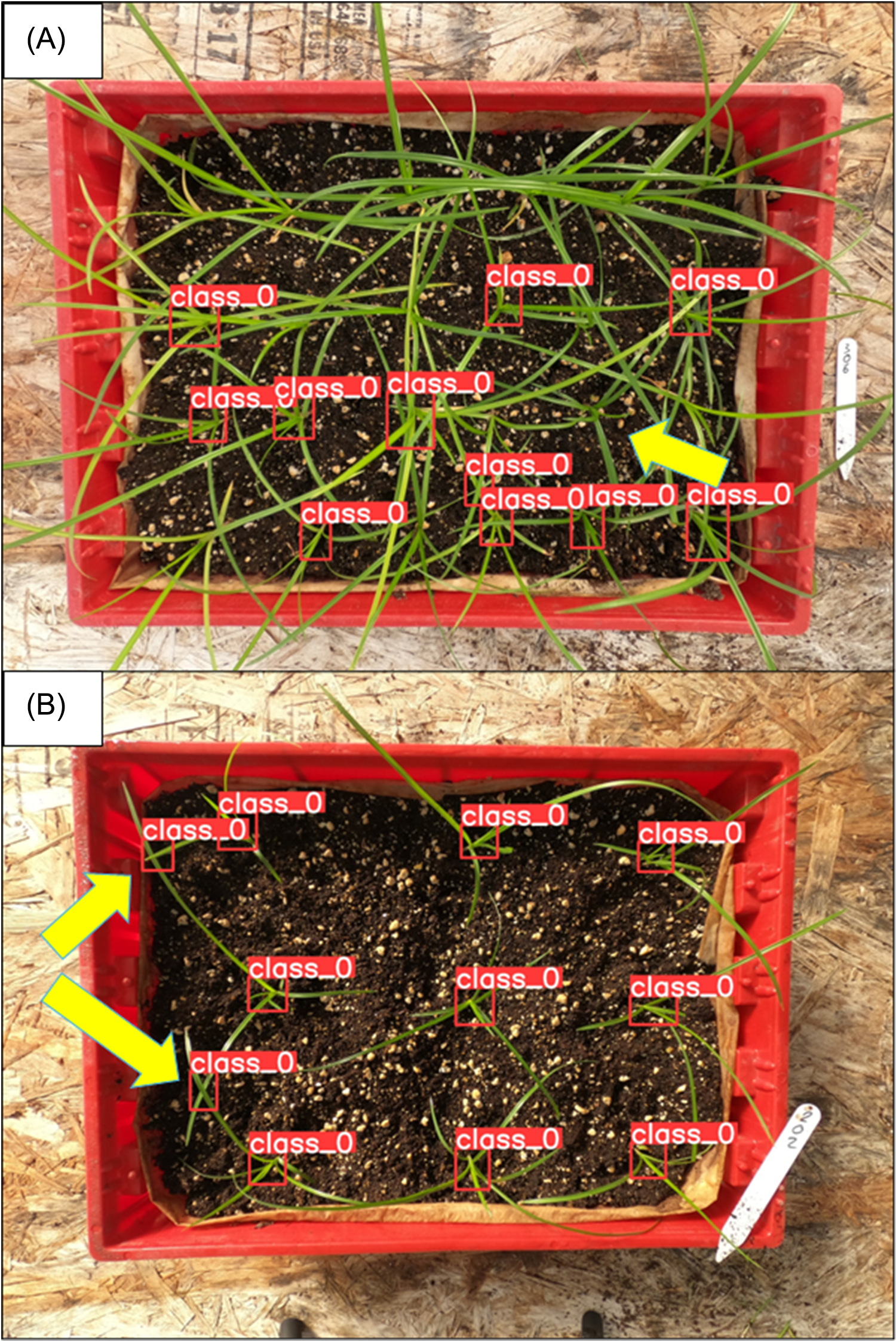
To address the impact of both density and canopy coverage, we selected two F1 score thresholds to identify the density at which these effects occur (Figure 6). The optimal model performance (OMP), defined as an F1 score ≥0.90, indicates strong model performance. In contrast, the marginal model performance (MMP), defined as an F1 score of 0.50, indicates that densities above this threshold result in unreliable model performance. At transplant, OMP was maintained up to a density of 157 plants m−2. This threshold decreased to 111 plants m−2 at 3 DATr, and further to 99 plants m−2 at 6 DATr, remaining consistent at 10 DATr. At 17 DATr, the OMP threshold dropped to 86 plants m−2. Despite the relatively unbalanced representation of the number of instances in the training dataset (Figure 4), the model maintained F1 scores above 0.90 across all densities corresponding to this range of instance counts. Similar performance was observed at considerably higher densities during early evaluations, when canopy coverage and occlusion were still limited. However, OMP decreased substantially as canopy coverage increased, suggesting that the decline in performance was primarily associated with overlapping vegetation, occlusion, and changes in plant morphology resulting from the increased proximity between plants, rather than the exclusion of higher instance counts from the training dataset. Furthermore, there was a consistent decline in the density for achieving the MMP threshold across changes in canopy coverage. At transplant, MMP was achieved at 322 plants m−2. This decreased to 244 plants m−2 at 3 DATr, 203 plants m−2 at 6 DATr, 182 plants m−2 at 10 DATr, and 140 plants m−2 at 17 DATr. The impact of changes in plant morphology and canopy coverage had a bigger effect on the density threshold to achieve MMP compared with achieving OMP. In contrast to the stabilization of OMP between 6 and 10 DATr, MMP is consistently influenced by greater canopy coverage. Although most false negatives were associated with increased overlap and occlusion of features at higher densities and greater canopy coverage, a few cases were observed where the basal leaf rosette was clear, but the model still failed to detect it, as illustrated in Figure 8A. These cases were relatively uncommon and may reflect limitations in model generalization.
Red bounding boxes indicate predictions made by the model. (A) Yellow arrow shows a model failure to detect the basal leaf rosette of Cyperus rotundus despite clear visibility. (B) Yellow arrows highlight false positives due to overlap between leaves.

The inflection point at transplant, where the F1 score began to decline most rapidly, occurred at 275 plants m−2, decreasing to 230 plants m−2 at 3 DATr. Inflection points further decreased to 203, 182, and 140 plants m−2 at 6, 10, and 17 DATr, respectively. The closer alignment of the inflection points with the MMP density thresholds as canopy coverage increased, along with the increased steepness, indicates that the model deteriorates significantly faster as density increases at later time points and suggests larger inaccuracies in density estimation by the model. This could result in a less reliable population map if there were severe C. rotundus infestation clusters in the field. Alternative strategies can be evaluated to address these limitations. For instance, a continuous density map could be generated by aggregating point-based estimates from multiple images covering a given area into larger grid cells, rather than relying solely on individual point data. Assigning density categories to each cell may help smooth out inaccuracies and provide a more robust representation of infestation severity. Unlike weed maps produced via semantic segmentation, which primarily quantify the proportion of ground area occupied by weeds, this density-based approach emphasizes the distribution and intensity of weed occurrences, allowing for a more detailed analysis of infestation patterns. Future research should employ datasets representing entire fields to enable a comprehensive evaluation of weed maps generated by ground-based detection models and explore methods that address inaccuracies under high-density scenarios.
Precision and Recall
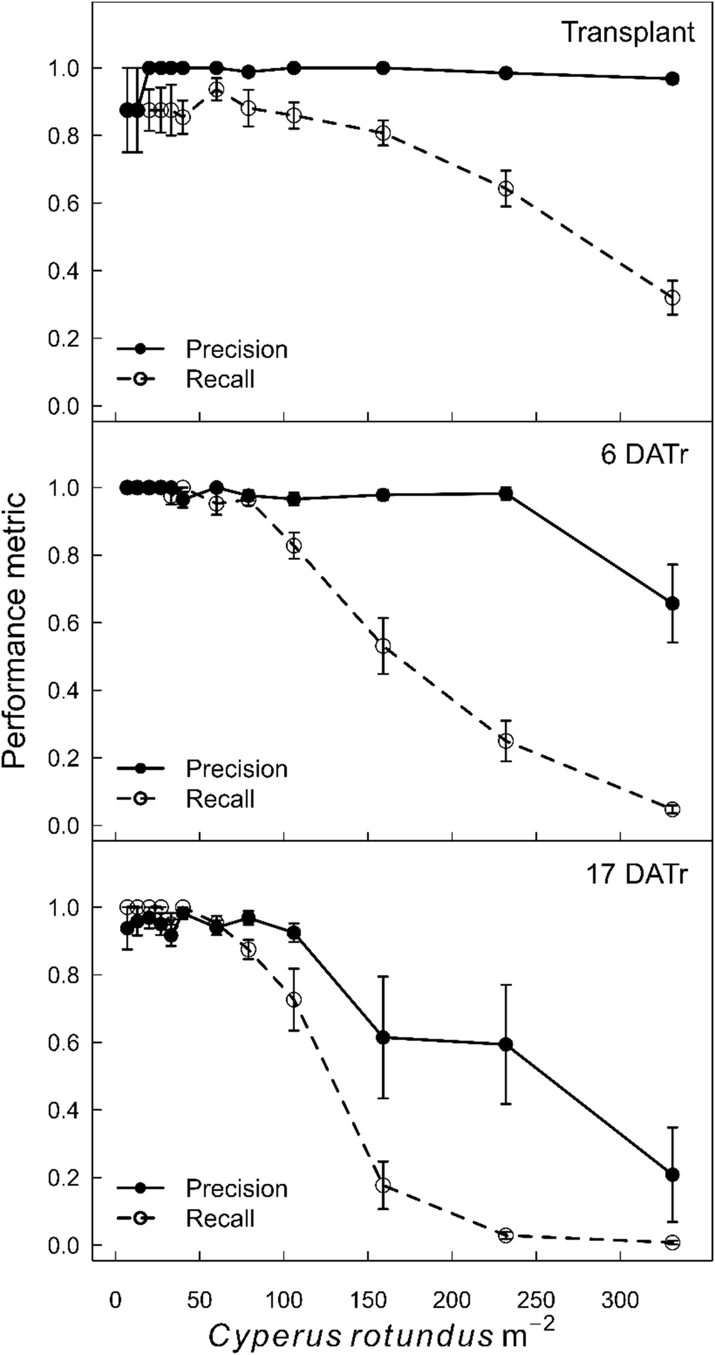
In weed mapping, a decline in the F1 score suggests inaccuracies in estimating weed density, but it is unclear whether this indicates an overestimation or underestimation of the weed population. Therefore, examining both precision and recall is crucial to understanding the nature of the decline in F1 score at increased densities of C. rotundus. Figure 9 illustrates how increasing C. rotundus density impacts the precision and recall of the model at transplant and 6 and 17 DATr. The primary factor impacting the model performance at higher densities of C. rotundus is the increase in false negatives, as evidenced by the sharper decline in recall at all time points. At transplant, there is a sharp decline in recall as the density increases, while precision remains consistently high. This indicates a significant increase in false negatives without a corresponding increase in false positives. A similar trend is observed at 6 DATr. However, there is a significant decrease in precision at 331 plants m−2, indicating an increase in false positives only at the highest density evaluated. At 17 DATr, both precision and recall decline significantly with increasing density, with recall still playing a more critical role in the F1 score decline as density increases. Most false positives occurred on overlapping C. rotundus leaves, potentially caused by shapes resembling the triangular arrangement of target structures (Figure 8B). This, along with the lower number of correct predictions, accounts for the drop in precision as density increases and plants grow larger. While overlapping leaves occasionally resulted in false detections, their frequency did not appear to increase with the degree of leaf overlap. This can be observed in Figure 8A, where despite a substantially higher level of overlap than in Figure 8B, no false positives were observed. Expanding the training data to include more overlapping conditions could help reduce such occurrences.
Precision and recall metrics at transplant and 6 and 17 d after transplanting (DATr), evaluated across varying Cyperus rotundus densities.

Another factor influencing the precision of our model is the absence of other weed species in the density test dataset, which was intentionally limited to a single species to minimize potential confounding factors. Buzanini et al. (Reference Buzanini, Schumann and Boyd2024) noted that a targeted sprayer, using a multi-class YOLO model trained to recognize Cyperus spp., grasses, and broadleaves, often produced false positives by misidentifying small, narrow-leaved grasses as Cyperus spp. Although our model was trained solely to detect Cyperus spp., other plants, including grass and broadleaf weed species, were present in the training data but were not annotated. However, the lack of weed diversity in the density test dataset may lead to an overestimation of precision. If other weed species were included, there could be an increase in false positives, resulting in lower precision and providing a more accurate evaluation of the model performance in natural, mixed-species environments. Therefore, creating density test datasets with different weed species could improve our approach to evaluating model robustness and enhance the assessment of multi-class weed detection models.
The ability of detection models to localize and distinguish individual weeds in images could support the generation of fine-scale weed maps in agricultural fields. However, the accuracy of these maps would depend heavily on the performance and reliability of the detection model. This study demonstrated that model performance is significantly influenced by the morphological characteristics of C. rotundus and the level of infestation. Model performance varied across different canopy coverage of C. rotundus; lower canopy coverage showed greater variability in accurate identification, while higher canopy coverage required lower density thresholds for optimal performance. The YOLOv8 extra-large model trained in this study demonstrated strong detection performance (F1 ≥ 0.90) at densities up to 157 plants m−2 when C. rotundus plants have three leaves. Under these conditions, marginal performance (F1 = 0.50) was observed at 322 plants m−2. While it is difficult to define exact density thresholds due to natural variability in C. rotundus growth and canopy overlap under field conditions, our findings suggest that under more challenging scenarios involving mature plants and dense infestations, optimal performance is maintained up to 86 plants m−2, with marginal performance occurring at 140 plants m−2. Timely field assessments are therefore crucial to map weeds before they grow larger and increase canopy coverage, ensuring reliable detection and supporting highly accurate weed maps. Although model accuracy could be improved by increasing training data to enhance feature identification under varied canopy conditions, feature occlusion common in dense infestations remains a substantial limitation. Therefore, field-specific validation of detection models and weed maps will remain essential, as additional factors beyond canopy coverage may influence overall mapping reliability. Future research should explore mixed–weed species density test datasets and evaluate different model versions and approaches, such as instance segmentation or transformer-based detectors, to identify differences in their ability to detect weeds under complex canopy conditions and varying infestation levels.
Acknowledgments
The authors would like to acknowledge Cecilia Lopez and Emily Witt for their technical assistance during experiment setup and data collection.
Funding statement
This project was funded by the Florida Strawberry Research and Education Foundation.
Competing interests
The authors declare no conflicts of interest.



 Open access

