Introduction

Over the last two decades considerable effort has been expended to develop convincing ice-sheet models. These range from two-dimensional, steady-stale snapshot models (e.g. Reference Whillans and JohnsenWhillans and Johnsen, 1983; Reference Waddington and ClarkeWaddington and Clarke, 1988; Reference Jóhannesson, Raymond and WaddingtonJóhannesson and others, 1989) to three-dimensional time-evolving thermomechanical models (e.g. Budd and Jenssen, 1989; Reference Huybrechts and CaschettoHuybrechts, 1993; Fahre and others, 1995; Reference Greve and HutterGreve and Hutter, 1995). Together, these models form a hierarchy of tools tuned to answer particular glaciological questions. While the trend is towards more complex models that include more mechanisms and interactions, it is arguably true that we have not yet fully exploited the simple models for the insight that they can provide into the behaviour of the ice sheet.

In this study we use a model that is simple in concept and application to predict the surface elevation of the ice sheet. While this model ignores many of the physical processes that would be required to reproduce the details of the ice flow, most notably basal topography and drag conditions, it can usefufly be considered as a zero-order model of the ice sheet. We then compare the predicted surface elevation with the best available continental DEM to highlight the grossest model/observation differences. Finally, we attempt to ascribe these gross distortions of the ice-sheet surface to known areas of basal sliding and rock outcrop.

Antarctic Digital Elevation Model: Observed Dem

This study arose from an attempt to assess a new digital elevation model (DEM) of Antarctica (Fig. 1) previously presented and discussed by Bamber (1994) and Bamber and Huybrechts (1996). For most of the continent, the DEM was derived from over 20000000 measurements of surface elevation retrieved from eight 35 day repeat cycles of the ERS-1 satellite radar altimeter. The spacing of satellite tracks and considerable footprint of the altimeter beam mean that short wavelength features are lost from the satellite altimetry, and the derived DEM is smoothed. Bamber (1994) estimated the random error in the altimeter measurements to be ±2.4 m, with similar magnitude for the biases. in areas of higher surface slope, accuracy is further reduced. Around the coast and in mountainous areas where the altimeter failed to maintain track on the ice-sheet surface, the altimeter measurements were supplemented with data taken from the Antarctic Digital Database (SCAR, 1993).

Beyond the orbital limit of ERS-1, south of 81.5°S, data from the Scott Polar Research Institute Folio Series (Reference Drewry, J. R. and DrewryDrewry, 1983) and data from the original airborne radar sounding flights have been used. in some areas the only data available were collected during the Tropical Wind Energy Conversion Reference Level Experiment (TW^rERLE) 1975-76 (Lcvanon and others, 1977; Reference LevanonLevanon, 1982). While being an order of magnitude less accurate than satellite altimetry, these data are still valuable, having a worst-case error of around ±60 m (Reference Levanon, Julian and SuomiLevanon and others, 1977).

Fig. 1. Location map for Antarctica, with areas of rock outcrop filled. 1. Institute Ice Stream, 2. Foundation Ice Stream, 3. Patuxent Ice Stream, 4. Amery Ice Shelf, 5. Bailey Ice Stream, 6. Slessor Ice Stream, 7. Evans Ice Stream, 8. Lambert Glacier, 9. Dome Argus, 10. Transantarctic Mountains, 11. Byrd Glacier, 12. David Glacier, 13. Siple Coast, 14. Pine Island Glacier, 15. Thwaites Glacier.

Fig. 2. Digital elevation model of Antarctica: the observed DEM. (a) Shaded surface relief with illumination from top of page. (b) Shaded surface relief with illumination from right side of page, (c) Shaded to show magnitude of surface slope, with steeper slopes shaded darker, (d) Shaded to show direction of surface slope.

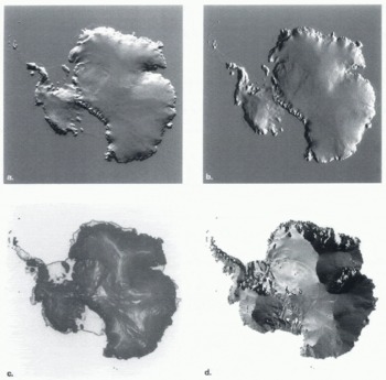
All these data were gridded to 10 km resolution using methods described by Bamber and Huybrechts (1996). Throughout the paper we shall refer to this DEM as the observed DEM. Figure 2 presents the observed DEM as a series of images designed to highlight complementary aspects of the topography. The two shaded-relief maps (Fig. 2a and b) give an impression of the overall shape of the ice sheet, while the map showing magnitude of surface slope (Fig. 2c) highlights flatter areas such as ridges, domes and lakes. Figure 2d shows the direction of maximum slope and serves to highlight the exact position of the ice divides and ridges.

Ice-Sheet Topography Models: Modelled Dem

The model of ice-sheet topography used in this study is the simple combination of two two-dimensional models. A plan-view model based on a continentality argument yields the shape of the predicted contours across the ice sheet. Elevations are then assigned to these contours using a theoretical two-dimensional ice-surface profile, to give a surface-elevation contour map of the predicted ice sheet. Interpolating the contours onto the same grid as the observed DEM gives the modelled DEM.

Continentality model

Reference MartinMartin (1976) gave a practical demonstration of the way that the positions of ice divides are controlled by the shape of the margins of the ice sheet. As an analogue of ice he used sand, which he poured onto a platform with a complex shape reminiscent of the bed beneath an ice rise. As the addition ofsand was gradual, a maximum load was eventually reached. in this state of self-ordered criticalily the maximum supportable surface slope was achieved everywhere, except for those areas very close to the crests of the ridges. The positions of the crests/divides in this maximal system were easily observed under low-angle illumination and shown to occur midway between the edges of the platform. in this demonstration the sand behaves as a plastic material, which can support only a certain maximum critical stress before failure, making it a reasonable first-order analogue of ice (Reference PatersonPaterson, 1994, ch. 5).

Reference ReehReeh (1982) formalised and extended this analysis and showed analytically, assuming a plastic rheology and the absence of a strong bedrock slope, that an ice divide should occur equidistant from the margins. He went on to show that for the central Greenland ice sheet there are significant departures from the idealised divide positions. He concluded that this was due to a strong trend in bedrock elevation, the positoni of the ice divide being drawn towards bedrock ridges.

The experiment performed by Martin can now be simulated digitally. Given the shape of the margin of an ice sheet, it is an easy procedure to draw “contours of continentality": normals are constructed inland from the grounding line, and continentality is defined as the distance along that normal to the grounding line. This was done for Berkner Island, Antarctica, by Vaughan and others (1996) who showed that the pattern of the divides predicted in this way was indeed very similar to that seen in reality. For the present study the margin is taken to be the grounding line extracted from the Antarctic Digital Database (SCAR, 1993). in this case the contours of continentality were drawn (Fig. 3a) using the “buffering” algorithm available in the ARC/ Info Geographical Information System (GIS), but also in many similar products. Contours of continentality correspond to the elevation contours predicted by Reeh's plastic ice-sheet model, assuming a flat ice-sheet bed.

Fig. 3. (a) Contours of continentality used as elevation contours to produce the modelled DEM. Generated from Antarctic Digital Database grounding line, buffered at 50 km intervals. The figure shows graphically that the Pole of Relative Inaccessibility for the contiguous continent is located at 82°50' S, 48°20' E (marked by triangle). This point is 1090 km away from that previously identified (marked by a star; BAS, 1993). (b) Ice flow drainage basins derived from observed DEM (full lines) and from contours of continentality (grey lines).

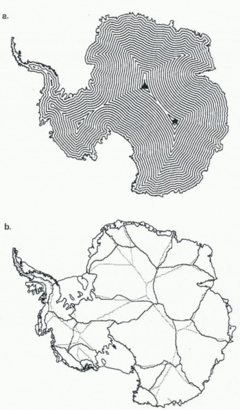
Figure 3b shows a comparison of the drainage basins predicted by the continentality model with those derived from the observed DEM (cf. Fig. 2d). in many areas the correspondence between the positions of modelled and observed DEMs is good, with the largest areas of mismatch occurring in Dronning Maud Land and West Antarctica.

Ice-sheet surface-elevation profile model

A two-dimensional ice-sheet profile model (Reference VialovVialov, 1958) was used to assign predicted surface elevations to the contours of continentality. Vialov (1958) showed that a model based on a power-law flow for ice yields a surface profile

where h is the ice-sheet surface elevation, H is surface elevation at the ice-sheet centre, x is the distance from the ice-sheet margin, and L is the distance from the ice-sheet centre to the margin. The flow-law parameter n is taken to be 3. We tunc the overall surface elevation by matching the elevation at the Pole of Relative Inaccessibility (Fig. 3a) to the elevation of Dome Argus (4050 m). Having applied this elevation profile to the contours of continentality we interpolated the contour map onto a grid, to produce the modelled DEM.

One inconsistency in the approach is that the model assumes a zero ice-sheet thickness at the ice-sheet margin, which is assumed to be the grounding line. Since ice thickness at the grounding line is not generally zero, there will be a model/observed mismatch near the grounding line. How-ever, the grounding-line ice thicknesses arealmost everywhere less than 2000 m, and around 1800 m of this is below sea level, so the mismatch due to this effect will only rarely exceed 200 m. We will see later that this is not significant compared to other sources of mismatch.

Below we shall present results for power-law flow. We have also produced a modelled DEM using a theoretical two-dimensional surface profile derived for plastic flow (Reference NyeNye, 1952), with very similar results. We therefore believe that our conclusions are largely insensitive to the choice of flow law.

Comparison of Observed Dem and Modelled Dem

Figure 4a and b shows the difference between observed DEM and modelled DEM. Only the areas of greatest mismatch (greater than +500m) are shaded, together with areas of mapped rock outcrop extracted from the Antarctic Digital Database (SCAR, 1993). The modelled DEM is on average only 300 m above the observed DEM. It is likely that accounting for variations in temperature and accumulation would have little effect on the model results, and we conclude that the gross areas of mismatch shown in Figure 4a and b are mainly the result of variations in bedrock conditions.

Areas for which observed DEM is higher than modelled DEM

Over much of the Antarctic ice sheet, the surface elevation does not closely reflect the topography of the bed that lies beneath it. in other words, the bed topography is generally buried so deep that it fails to redirect the ice flow at the surface. This can be seen by comparing the flowlines and bed-rock topography given by Drewry (1983) and Drewry and Jordan (1983). This is, however, not the case where the bed protrudes through the ice-sheet surface, forming an outcrop or nunatak; here the ice flow is necessarily diverted around the bed obstacle. Two effects cause outcrops to dam the ice flow and raise the icc-shcet surface upstream of outcrops. First, flow past the outcrop is genuinely obstructed and so the ice is at least partially dammed in the interior. To drive the ice through gaps between the outcrops requires a large local surface slope. Secondly, where ice flow is diverted around the outcrop, the actual distance which the ice must travel to reach the grounding line is increased. Here continentality underestimates the distance ice must flow to reach the grounding line. The ice surface is thus higher than would be predicted by the model used here, which causes an apparent damming. Together these two effects are largely responsible for the areas shown in Figure 4a, where the observed ice-sheet surface elevation is more than 500 m higher than the predicted surface elevations.

Fig. 4. Areas of difference between observed DEM and modelled DEM. (a) Areas where observed DEM is more than 500 m higher than modelled DEM (grey), with areas of rock outcrop (black) and extent of ERS-1 altimetry (circle) and drainage basins (full lines), (b) Areas where observed DEM is more than 500 m lower than modelled DEM (grey), and extent of ERS-1 altimetry (circle) and drainage basins (full lines). The labels identify areas discussed in the text.

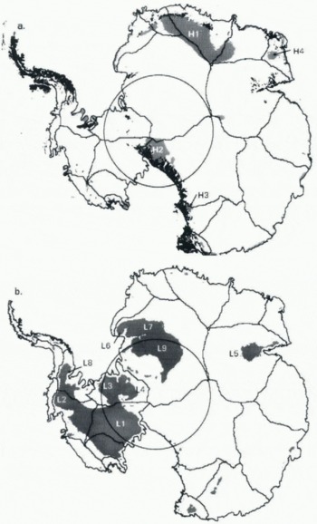
Areas HI, H2, H3 are directly upstream of extensive areas of rock outcrop associated with extensive mountain ranges. The distributions of these areas shows up several noteworthy points. The damming effect of mountain ranges in Dronning Maud Land (HI) appears to reach back into the drainage basin and beyond the ice divide into the neighbouring basins. The area of damming produced by the Transantarctic Mountains is not continuous, and the large glaciers that cut through the range (e.g. Byrd Glacier, David Glaciery appear to be powerful enough to lower ice-surface elevation on their hinterlands.

Area H4 and some smaller unlabelled areas on coastal promontories are not so easily interpreted as the result of damming by rock outcrops; rather, they are probably associated with elevated areas of bedrock.

L9: A Low-Profile Ice Sheet in East Antarctica?

almost all the areas of damming and areas of low-profile ice sheet identified in this exercise are easily explained in terms of known outcrops and known or suspected basal lubrication. Only area L9, an extensive region (250 000 km²) of low-profile ice sheet within East Antarctica, remains unexplained. Such a large area of low-profile ice sheet has hitherto only been found in West Antarctica, where it is believed to be caused by massive ice-stream activity and basal lubrication. If L9 is the result of similar processes then it might cause us to rethink our ideas about the stability of the East Antarctic ice sheet.

It should be noted that much of area L9 lies beyond the limit of the ERS-1 altimeter data, and so the observed DEM in this region is less precise than elsewhere. Over this area it is derived largely from TWERLE balloon data, with a worst-case error of ±60 m (Levanon and others, 1977). Thus, while the inaccuracy of the observed DEM in this area may contribute to the surface-elevation anomaly, it is unlikely that it can account for most of the difference between observed DEM and modelled DEM (>500m). in the event that L9 is the result of defective TWERLE balloon data, then this in itself constitutes a substantial result when we remember flow many other studies have directly or indirectly relied on these data.

Figure 3 shows that the positions of the modelled and observed ice divides exhibit greatest disagreement in the basin containing L9. This is, however, not a significant factor in disturbing the modelled elevations in L9, for two reasons. First, at any point on the ice sheet only the downstream distance to the grounding line is significant in determining the model elevation. Thus application oi the observed ice-divide position in the model would cause no change in the modelled DEM in L9. Secondly, as surface slopes are low close to the ice divides of East Antarctica, divide position is sensitive to even modest differences in elevation.

We have found very few data of any type collected in this area which might confirm the interpretation of arca L9. Only a few ice-thickness measurements areavailable, and so ice-bed elevation maps have been compiled from only a handful of points (e.g. Drewry and Jordan, 1983). Furthermore, no ice-velocity measurements appear to be available. There does, however, appear to be some corroborative evidence available from other modelling studies.

An area approximately corresponding to L9 was identified as having an unusually high sliding fraction by the model fitting of Reference Fastook and PrenticeFastook and Prentice (1994). A similar effect can be seen in the results of Huybrechts (1993, fig. 7) where it was interpreted as a region of anomalously high basal temperature. in neither of these studies was the area explained or discussed in any particular detail, or even noted as being contrary to current wisdom.

Budd and Warner (1996) used an ice-surface DEM derived from Drewry (1983) to calculate the ice flux required to balance observed surface accumulation data over the entire ice sheet. Their map of balance fluxes (Budd and Warner, 1996, fig. 1) does appear to show an area of high ice flux roughly coinciding with area L9. It is not, however, correct to simply interpret this high flux as high velocity, when the ice thickness is so poorly known. Furthermore, since Budd and Warner's DEM and the observed DEM were derived largely from the same data in this area, the two efforts cannot be seen as entirely independent results.

Clearly, area L9 deserves the attention of fieldworkers but would require a high logistical commitment. Perhaps the best hope for obtaining the required velocity data in the near future will come from the Canadian satellite Radarsat which carries a synthetic aperture radar (SAR). Il has already been shown that fracture produced at ice-stream margins is visible in SAR imagery (Vaughan and others, 1994) and that ice-stream velocities can be derived from SAR images (Reference Goldstein, Engelhardt, Kamb and FrolichGoldstein and others, 1993). Radarsat is scheduled to be reconfigured to acquire complete Antarctic coverage in September 1997.

Conclusions

This study has shown the value of even simple models when used in conjunction with good observational data, especially on a continental scale. in general, the results of the comparison are confirmation of our intuitive expectations based on known regional flow characteristics. Rock out-crops have a damming effect on the ice sheet which may dramatically shift the ice divide. Conversely, areas of basal sliding lower the ice-sheet surface and give rise to low-profile ice sheets. The study has, however, been of further value, since it has identified an extensive region of low-profile ice sheet reaching into the heart of the East Antarctic ice sheet (area L9), which needs to be checked by some other method at the earliest possible date.