





1. Introduction
Görtler vortices are streamwise-aligned vortical structures that arise within the boundary layer over a concave wall (Görtler Reference Görtler1940). Their significance, extensively reviewed for example by Floryan (Reference Floryan1991), Saric (Reference Saric1994) and Xu, Ricco & Duan (Reference Xu, Ricco and Duan2024a ), continues to draw attention due to their critical role for the design of high-speed vehicles and jet engines (Es-Sahli et al. Reference Es-Sahli, Sescu, Afsar and Hattori2022; Li, Choudhari & Paredes Reference Li, Choudhari and Paredes2022; Xu, Ricco & Marensi Reference Xu, Ricco and Marensi2024b ; Zhang, Hao & Uy Reference Zhang, Hao and Uy2025). Pioneering experiments by Swearingen & Blackwelder (Reference Swearingen and Blackwelder1987), hereafter referred to as SB87, demonstrated that the downstream transition process involves the gradual development of Görtler vortices, followed by the emergence of short-scale wavy fluctuations that eventually break down into turbulence. Although the initial stages of the transition process are relatively well understood, a complete understanding has not yet been achieved.
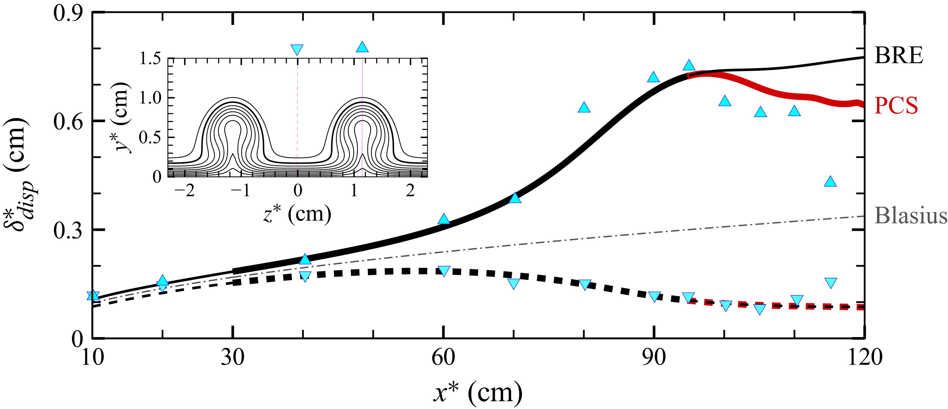
Displacement boundary layer thickness $\delta ^*_{\textit{disp}}$
measured at the spanwise locations corresponding to the peaks (up triangle, solid lines) and valleys (down triangle, dashed lines) of the Görtler vortices. The symbols are the experimental results taken from figure 9 of SB87, while the lines show our computational results. The inset shows the streamwise velocity from the BRE computation at
$\delta ^*_{\textit{disp}}$
measured at the spanwise locations corresponding to the peaks (up triangle, solid lines) and valleys (down triangle, dashed lines) of the Görtler vortices. The symbols are the experimental results taken from figure 9 of SB87, while the lines show our computational results. The inset shows the streamwise velocity from the BRE computation at $x^*=90$
cm (in the same format as figure 4). The magenta lines and symbols indicate the positions of the peaks and valleys of the mushroom-shaped vortices.
$x^*=90$
cm (in the same format as figure 4). The magenta lines and symbols indicate the positions of the peaks and valleys of the mushroom-shaped vortices.

Asymptotic analysis has long been an invaluable tool for examining the initial stages of transition. A milestone was Hall (Reference Hall1983), who pointed out that unless the local Görtler number is sufficiently large, linear growth of Görtler vortices could not be determined solely from the eigenvalue analysis of the local flow field. In such cases, numerical integration of a parabolic leading order problem along the streamwise direction is necessary. Hall (Reference Hall1988) solved the nonlinear version of the spatial-marching problem, which is now known as the boundary region equations (BRE). As shown by the black line in figure 1, the BRE predictions agree remarkably well with the experiments of SB87 (symbols) up to a certain streamwise location.
In the numerical boundary layer community, the discrepancy in figure 1 beginning at $x^*=$
95 cm is believed to be caused, at least in part, by secondary instability. Hall & Horseman (Reference Hall and Horseman1991) showed that when nonlinear Görtler vortices emerge, the streamwise velocity exhibits pronounced streaky modulations, which in turn trigger inviscid instabilities. In subsequent studies, spatial marching computations of Görtler vortices, combined with their local linear stability analysis, have become a standard framework (Yu & Liu Reference Yu and Liu1994; Li & Malik Reference Li and Malik1995; Girgis & Liu Reference Girgis and Liu2006; Ren & Fu Reference Ren and Fu2015; Xu, Zhang & Wu Reference Xu, Zhang and Wu2017). However, stability analysis applies only to very small wave amplitudes and no quantitative study has examined the nonlinear effects of finite-amplitude waves on the flow.
$x^*=$
95 cm is believed to be caused, at least in part, by secondary instability. Hall & Horseman (Reference Hall and Horseman1991) showed that when nonlinear Görtler vortices emerge, the streamwise velocity exhibits pronounced streaky modulations, which in turn trigger inviscid instabilities. In subsequent studies, spatial marching computations of Görtler vortices, combined with their local linear stability analysis, have become a standard framework (Yu & Liu Reference Yu and Liu1994; Li & Malik Reference Li and Malik1995; Girgis & Liu Reference Girgis and Liu2006; Ren & Fu Reference Ren and Fu2015; Xu, Zhang & Wu Reference Xu, Zhang and Wu2017). However, stability analysis applies only to very small wave amplitudes and no quantitative study has examined the nonlinear effects of finite-amplitude waves on the flow.
In this paper, we addresses this challenge using the parabolised coherent structures (PCS) method recently proposed by Song & Deguchi (Reference Song and Deguchi2025). To incorporate the feedback from fast-scale finite-amplitude waves into the slowly developing vortices within a spatial marching scheme, the PCS couples the BRE with the computation of exact coherent structures. This approach is motivated by recent studies of parallel shear flows (Wang, Gibson & Waleffe Reference Wang, Gibson and Waleffe2007; Hall & Sherwin Reference Hall and Sherwin2010; Deguchi & Hall Reference Deguchi and Hall2014b ), which revealed that simple nonlinear Navier–Stokes solutions (i.e. exact coherent structures) embody the vortex–wave interaction (VWI, Hall & Smith Reference Hall and Smith1991), also known as the self-sustaining process of coherent structures (Hamilton, Kim & Waleffe Reference Hamilton, Kim and Waleffe1995; Waleffe Reference Waleffe1997). Our aim is to demonstrate that the detailed understanding of coherent structures accumulated within the asymptotic and dynamical systems theory community is indeed useful for explaining experimental results by SB87, even beyond the point at which secondary instabilities arise.
The paper is organised as follows. Section 2 presents the formulation of the PCS, along with its justification via asymptotic analysis and the details of the computational set-up. Section 3 reports the computational results and compares them with the experiment of SB87. We mainly use experimental data because incompressible direct numerical simulation (DNS) studies that record wave amplitudes are rare; one such exception is Souza (Reference Souza2017). Finally, § 4 briefly discusses the implications of our computations.
2. Formulation of the problem
Consider a boundary layer developing over a concave wall with a dimensional radius of curvature $a^*$
. The incompressible Navier–Stokes equations in cylindrical coordinates
$a^*$
. The incompressible Navier–Stokes equations in cylindrical coordinates $(r^*,\theta ,z^*)$
serve as the starting point of our analysis. In boundary layer flows, the Reynolds number is typically defined as
$(r^*,\theta ,z^*)$
serve as the starting point of our analysis. In boundary layer flows, the Reynolds number is typically defined as $\textit{Re}={U_{\infty }^*L^*}/{\nu ^*}$
, where
$\textit{Re}={U_{\infty }^*L^*}/{\nu ^*}$
, where $U_{\infty }^*$
is the free strem velocity,
$U_{\infty }^*$
is the free strem velocity, $L^*$
is a characteristic streamwise length scale and
$L^*$
is a characteristic streamwise length scale and $\nu ^*$
is the kinematic viscosity of the fluid. The flow field is assumed to be periodic in
$\nu ^*$
is the kinematic viscosity of the fluid. The flow field is assumed to be periodic in $z^*$
with a period of
$z^*$
with a period of $\lambda ^*$
.
$\lambda ^*$
.
By using the characteristic boundary layer thickness $\delta ^*=\textit{Re}^{-1/2}L^*$
as the length scale,
$\delta ^*=\textit{Re}^{-1/2}L^*$
as the length scale, $U_{\infty }^*$
as the velocity scale and the fluid density
$U_{\infty }^*$
as the velocity scale and the fluid density $\rho ^*$
as the density scale, one obtains the Navier–Stokes equations for the velocity
$\rho ^*$
as the density scale, one obtains the Navier–Stokes equations for the velocity $\boldsymbol{u}=u_r\boldsymbol{e}_r+u_{\varphi }\boldsymbol{e}_{\varphi }+u_z\boldsymbol{e}_z$
and pressure
$\boldsymbol{u}=u_r\boldsymbol{e}_r+u_{\varphi }\boldsymbol{e}_{\varphi }+u_z\boldsymbol{e}_z$
and pressure $p$
fields. In this well-known non-dimensional formulation in
$p$
fields. In this well-known non-dimensional formulation in $(r,\varphi ,z)$
, where
$(r,\varphi ,z)$
, where $r=r^*/\delta ^*$
and
$r=r^*/\delta ^*$
and $z=z^*/\delta ^*$
, the viscous terms appear multiplied by
$z=z^*/\delta ^*$
, the viscous terms appear multiplied by $1/R_{\delta }$
, where
$1/R_{\delta }$
, where $R_{\delta }$
is the Reynolds number based on the boundary layer thickness:
$R_{\delta }$
is the Reynolds number based on the boundary layer thickness:
 \begin{eqnarray} R_{\delta }=\frac {U_{\infty }^*\delta ^*}{\nu ^*}=\textit{Re}^{1/2}. \end{eqnarray}
Further, setting $[u,v,w]=[u_{\varphi },u_r,u_z]$
,
$[u,v,w]=[u_{\varphi },u_r,u_z]$
, $y=r-a$
and
$y=r-a$
and $x=a\varphi$
with
$x=a\varphi$
with $a=a^*/\delta ^*$
, the governing equations are recast in a suitable coordinate system that forms the basis for deriving the reduced equations for the PCS. For convenience, we introduce
$a=a^*/\delta ^*$
, the governing equations are recast in a suitable coordinate system that forms the basis for deriving the reduced equations for the PCS. For convenience, we introduce $x^*=\delta ^*x$
, which represents the dimensional distance from the leading edge.
$x^*=\delta ^*x$
, which represents the dimensional distance from the leading edge.
The VWI theory by Hall & Smith (Reference Hall and Smith1991) and Hall & Sherwin (Reference Hall and Sherwin2010) provides the most rational way to identify the dominant terms in the governing equations when $\textit{Re}\gg 1$
. However, numerical computation of the resulting leading-order system is highly challenging. As we shall see in § 2.2, the PCS method therefore employs a reduced system that lies between the full equations and the VWI system. In other words, the PCS retains some higher-order terms, which is advantageous both for simplifying numerical computations and for improving accuracy of the approximation (see Song & Deguchi Reference Song and Deguchi2025).
$\textit{Re}\gg 1$
. However, numerical computation of the resulting leading-order system is highly challenging. As we shall see in § 2.2, the PCS method therefore employs a reduced system that lies between the full equations and the VWI system. In other words, the PCS retains some higher-order terms, which is advantageous both for simplifying numerical computations and for improving accuracy of the approximation (see Song & Deguchi Reference Song and Deguchi2025).
2.1. Vortex–wave interaction
In the VWI theory, the velocity and pressure fields are decomposed as
 \begin{eqnarray} [\boldsymbol{u},p]=[\overline {\boldsymbol{u}},\overline {p}](X,y,z)+[\tilde {\boldsymbol{u}}, { \tilde {p}]}(X,\theta ,y,z), \end{eqnarray}
using the slow variable $X=R_{\delta }^{-1}x=x^*/L^*$
and the fast phase variable
$X=R_{\delta }^{-1}x=x^*/L^*$
and the fast phase variable
 \begin{eqnarray} \theta =R_{\delta }\int ^X_0 \alpha (s)\,{\rm d}s- \varOmega t. \end{eqnarray}
Here, $\alpha (X)$
is the local wavenumber and
$\alpha (X)$
is the local wavenumber and $\varOmega$
is the frequency; both are assumed to be real-valued. The overline denotes the steady vortex part, while the tilde denotes the time-dependent wave part; their asymptotic expansions are given by
$\varOmega$
is the frequency; both are assumed to be real-valued. The overline denotes the steady vortex part, while the tilde denotes the time-dependent wave part; their asymptotic expansions are given by
 \begin{eqnarray} [\overline {u},\overline {v},\overline {w},\overline {p}]&=& \big[U,R_{\delta }^{-1}V,R_{\delta }^{-1}W,R_{\delta }^{-2}P\big](X,y,z)+{\cdots} , \end{eqnarray}
 \begin{eqnarray} [\tilde {\boldsymbol{u}},\tilde {p}]&=&\epsilon ^{1/2} R_{\delta }^{-1}e^{i\theta }[\hat {\boldsymbol{u}},\hat {p}](X,y,z)+\text{c.c.}+{\cdots} , \end{eqnarray}
where c.c. stands for complex conjugate and $\epsilon =R_{\delta }^{-1/3}$
denotes the critical layer thickness. In the self-sustaining process,
$\epsilon =R_{\delta }^{-1/3}$
denotes the critical layer thickness. In the self-sustaining process, $U$
and
$U$
and $[V,W]$
are referred to as the streak and roll components, respectively. As shown by Hall & Smith (Reference Hall and Smith1991) and Hall & Sherwin (Reference Hall and Sherwin2010), a wave amplitude of
$[V,W]$
are referred to as the streak and roll components, respectively. As shown by Hall & Smith (Reference Hall and Smith1991) and Hall & Sherwin (Reference Hall and Sherwin2010), a wave amplitude of $O(R_{\delta }^{-7/6})$
is required to drive
$O(R_{\delta }^{-7/6})$
is required to drive $O(1)$
streaks.
$O(1)$
streaks.
By substituting (2.4) into the governing equations, defining the Görtler number as $G=2R_{\delta }^2/a$
and retaining only the leading-order terms, we obtain
$G=2R_{\delta }^2/a$
and retaining only the leading-order terms, we obtain
 \begin{eqnarray} \big[U\partial _X +V\partial _y +W\partial _z-\partial _y^2-\partial _z^2\big] \left [ \begin{array}{c} U\\ V\\ W \end{array} \right ] + \left [ \begin{array}{c} 0\\[3pt] \partial _y P+ \textit{GU}^2/2 \\[3pt] \partial _z P \end{array} \right ] =\boldsymbol{F},\quad \end{eqnarray}
 \begin{eqnarray} \partial _XU+\partial _yV+\partial _zW=0,\quad \end{eqnarray}
from the mean part and
 \begin{eqnarray} i\alpha (U-c)\hat {u}+\hat {v}\partial _y U+\hat {w}\partial _z U=-i\alpha \hat {p},\quad i\alpha (U-c)\hat {v}=-\partial _y \hat {p}, \end{eqnarray}
 \begin{eqnarray} i\alpha (U-c)\hat {w}=-\partial _z \hat {p},\quad i\alpha \hat {u}+\partial _y\hat {v}+\partial _z\hat {w}=0, \end{eqnarray}
from the fluctuation part. The right-hand side of (2.5) is the Reynolds stress produced by the wave and we retain the higher-order terms for later use; without this term, (2.5) reduces to the BRE used by Hall (Reference Hall1988). While (2.6) represents the inviscid secondary instability equations used by Hall & Horseman (Reference Hall and Horseman1991), with $c(X)=\varOmega /\alpha (X)$
being the local phase speed, this quantity is real-valued, according to the assumption stated just after (2.3).
$c(X)=\varOmega /\alpha (X)$
being the local phase speed, this quantity is real-valued, according to the assumption stated just after (2.3).
Careful analysis shows that the feedback from the wave to the roll-streak field occurs solely within the critical layer of thickness $\epsilon$
, which regularises the singularity of (2.6) at
$\epsilon$
, which regularises the singularity of (2.6) at $U=c$
by reintroducing the viscous effect. The method of Frobenius expansion shows that the eigenfunction of the inviscid wave problem becomes singular (see e.g. Deguchi Reference Deguchi2019). The regularised wave within the critical layer thus acquires a larger size and the magnitude of
$U=c$
by reintroducing the viscous effect. The method of Frobenius expansion shows that the eigenfunction of the inviscid wave problem becomes singular (see e.g. Deguchi Reference Deguchi2019). The regularised wave within the critical layer thus acquires a larger size and the magnitude of $\boldsymbol{F}$
increases accordingly. After a long algebra, it can be shown that the Reynolds stress term affects
$\boldsymbol{F}$
increases accordingly. After a long algebra, it can be shown that the Reynolds stress term affects $V,W,P$
through jump conditions across the critical layer (see (2.15) and (B16) of Song & Deguchi Reference Song and Deguchi2025, for example). The
$V,W,P$
through jump conditions across the critical layer (see (2.15) and (B16) of Song & Deguchi Reference Song and Deguchi2025, for example). The $\epsilon ^{1/2}$
factor in (2.4) arises from the stress balance within the critical layer.
$\epsilon ^{1/2}$
factor in (2.4) arises from the stress balance within the critical layer.
The jump conditions, together with the BRE and (2.6), form a closed system determining the leading-order approximation of the solution. However, numerical computation of this problem requires handling the singular behaviour of the solutions at the critical layer, whose location is not known a priori. For this reason, even more than 30 years after the leading-order problem was derived for boundary-layer flows by Hall & Smith (Reference Hall and Smith1991), no solution has yet been obtained.
2.2. Parabolised coherent structures method
In the PCS approach, the jump conditions in the VWI are replaced by the Reynolds stress
 \begin{eqnarray} \boldsymbol{F}=-[R_{\delta }\overline {(\tilde {\boldsymbol{u}}\boldsymbol{\cdot }\tilde {\boldsymbol{\nabla }})\tilde {u}},R_{\delta }^2\overline {(\tilde {\boldsymbol{u}}\boldsymbol{\cdot }\tilde {\boldsymbol{\nabla }})\tilde {v}},R_{\delta }^2\overline {(\tilde {\boldsymbol{u}}\boldsymbol{\cdot }\tilde {\boldsymbol{\nabla }})\tilde {w}}], \end{eqnarray}
and (2.6) is replaced by
 \begin{eqnarray} (\overline {\boldsymbol{u}}\boldsymbol{\cdot }\tilde {\boldsymbol{\nabla }}-c\alpha \partial _{\theta })\tilde {\boldsymbol{u}}+ (\tilde {\boldsymbol{u}}\boldsymbol{\cdot }\tilde {\boldsymbol{\nabla }})\overline {\boldsymbol{u}} +(\tilde {\boldsymbol{u}}\boldsymbol{\cdot }\tilde {\boldsymbol{\nabla }})\tilde {\boldsymbol{u}}-\overline {(\tilde {\boldsymbol{u}}\boldsymbol{\cdot }\tilde {\boldsymbol{\nabla }})\tilde {\boldsymbol{u}}} =-\tilde {\boldsymbol{\nabla }}\! \tilde {p}+R_{\delta }^{-1}\tilde {{\nabla} }^2 \tilde {\boldsymbol{u}},\quad \end{eqnarray}
 \begin{eqnarray} \tilde {\boldsymbol{\nabla }}\boldsymbol{\cdot }\tilde {\boldsymbol{u}}=0,\quad \end{eqnarray}
where $\tilde {\boldsymbol{\nabla }}=[\alpha \partial _{\theta },\partial _y,\partial _z]$
. The PCS approach solves (2.5), (2.7) and (2.8) with
$\tilde {\boldsymbol{\nabla }}=[\alpha \partial _{\theta },\partial _y,\partial _z]$
. The PCS approach solves (2.5), (2.7) and (2.8) with $[\overline {u},\overline {v},\overline {w},\overline {p}]=[U,R_{\delta }^{-1}V,R_{\delta }^{-1}W,R_{\delta }^{-2}P]$
. The PCS system can be derived directly from the Navier–Stokes equations by making the following assumptions: (i) the effect of wall curvature on the flow field enters solely through the so-called Görtler term; (ii) the mean part of the governing equations can be parabolised; and (iii) derivatives with respect to the slow variable
$[\overline {u},\overline {v},\overline {w},\overline {p}]=[U,R_{\delta }^{-1}V,R_{\delta }^{-1}W,R_{\delta }^{-2}P]$
. The PCS system can be derived directly from the Navier–Stokes equations by making the following assumptions: (i) the effect of wall curvature on the flow field enters solely through the so-called Görtler term; (ii) the mean part of the governing equations can be parabolised; and (iii) derivatives with respect to the slow variable $X$
can be neglected when acting on the fluctuation components.
$X$
can be neglected when acting on the fluctuation components.
The PCS system possesses some remarkable properties. First, its asymptotic analysis yields the same leading-order VWI system. Thus, the PCS computes approximate solutions when $\textit{Re}\gg 1$
. A detailed discussion on the relationship between the VWI theory and the PCS method can be found in Song & Deguchi (Reference Song and Deguchi2025). As discussed in that paper, assumptions (i)–(iii) can be justified through asymptotic analysis (note that some higher order terms are retained in (2.7) and (2.8)). Second, the PCS formulation allows spatial marching (i.e. integration in
$\textit{Re}\gg 1$
. A detailed discussion on the relationship between the VWI theory and the PCS method can be found in Song & Deguchi (Reference Song and Deguchi2025). As discussed in that paper, assumptions (i)–(iii) can be justified through asymptotic analysis (note that some higher order terms are retained in (2.7) and (2.8)). Second, the PCS formulation allows spatial marching (i.e. integration in $X$
), similar to the BRE. Hence, the numerical computation is significantly more efficient than obtaining a statistically steady state via a DNS. Third, if the system is independent of
$X$
), similar to the BRE. Hence, the numerical computation is significantly more efficient than obtaining a statistically steady state via a DNS. Third, if the system is independent of $X$
, as is the case in parallel flows, travelling-wave solutions of the Navier–Stokes equations satisfy it exactly. This allows the self-sustaining process of exact coherent structures to be naturally incorporated into spatial marching. Fourth, under the constant freestream speed considered here, the system admits the Blasius boundary-layer solution. The PCS, therefore, do not require artificial forcing to maintain the base flow, unlike local periodic box computations of spatially developing flows (e.g. Kozul, Chung & Monty Reference Kozul, Chung and Monty2016; Ruan & Blanquart Reference Ruan and Blanquart2021).
$X$
, as is the case in parallel flows, travelling-wave solutions of the Navier–Stokes equations satisfy it exactly. This allows the self-sustaining process of exact coherent structures to be naturally incorporated into spatial marching. Fourth, under the constant freestream speed considered here, the system admits the Blasius boundary-layer solution. The PCS, therefore, do not require artificial forcing to maintain the base flow, unlike local periodic box computations of spatially developing flows (e.g. Kozul, Chung & Monty Reference Kozul, Chung and Monty2016; Ruan & Blanquart Reference Ruan and Blanquart2021).
Using an implicit finite-difference scheme in the $X$
-direction, updating the fields is equivalent to solving a travelling-wave problem in a parallel flow, with contributions from the previous step treated as a forcing term. Thus, Song & Deguchi (Reference Song and Deguchi2025) build on a code that computes exact coherent structures by finding the root of a discretised system using the Newton–Raphson method. The descretisation uses Fourier–Galerkin in the
$X$
-direction, updating the fields is equivalent to solving a travelling-wave problem in a parallel flow, with contributions from the previous step treated as a forcing term. Thus, Song & Deguchi (Reference Song and Deguchi2025) build on a code that computes exact coherent structures by finding the root of a discretised system using the Newton–Raphson method. The descretisation uses Fourier–Galerkin in the $\theta$
and
$\theta$
and $z$
directions, and Chebyshev collocation in the
$z$
directions, and Chebyshev collocation in the $y$
direction.
$y$
direction.
In addition to the modifications due to the finite-difference in the $X$
-direction, a few more adjustments are necessary. In the numerical computations, the
$X$
-direction, a few more adjustments are necessary. In the numerical computations, the $y$
-domain must be truncated at a finite value
$y$
-domain must be truncated at a finite value $H$
. For accurate computation,
$H$
. For accurate computation, $H$
must be chosen large enough while ensuring sufficient resolution within the boundary layer. To satisfy both requirements, the Chebyshev expansion is first performed in
$H$
must be chosen large enough while ensuring sufficient resolution within the boundary layer. To satisfy both requirements, the Chebyshev expansion is first performed in $Y\in [-1,1]$
and then mapped to
$Y\in [-1,1]$
and then mapped to $y\in [0,H]$
via
$y\in [0,H]$
via $y=({\textit{HB}(1+Y)})/({(1-Y)H+2\textit{BY}})$
. By choosing the constant
$y=({\textit{HB}(1+Y)})/({(1-Y)H+2\textit{BY}})$
. By choosing the constant $B$
to be sufficiently smaller than
$B$
to be sufficiently smaller than $H/2$
, the Chebyshev collocation points can be clustered near the wall at
$H/2$
, the Chebyshev collocation points can be clustered near the wall at $y=0$
. No-slip boundary conditions are imposed at
$y=0$
. No-slip boundary conditions are imposed at $y=0,H$
on the perturbation to the Blasius boundary layer.
$y=0,H$
on the perturbation to the Blasius boundary layer.
Also, in the Newton method for exact coherent structures, $\alpha$
is prescribed and
$\alpha$
is prescribed and $c$
is obtained as part of solution. In the PCS, however, the product
$c$
is obtained as part of solution. In the PCS, however, the product $\alpha c$
must equal to the prescribed constant
$\alpha c$
must equal to the prescribed constant $\varOmega$
, which provides a natural update condition for
$\varOmega$
, which provides a natural update condition for $\alpha (X)$
. It should also be noted that, unlike in the parabolised stability equations (PSE) approach,
$\alpha (X)$
. It should also be noted that, unlike in the parabolised stability equations (PSE) approach, $\alpha$
is purely real. A brief comment on the difference between the BRE and the PSE can be found in Xu & Wu (Reference Xu and Wu2021) and Song & Deguchi (Reference Song and Deguchi2025).
$\alpha$
is purely real. A brief comment on the difference between the BRE and the PSE can be found in Xu & Wu (Reference Xu and Wu2021) and Song & Deguchi (Reference Song and Deguchi2025).
2.3. Computational set-up
To simulate the experimental conditions of SB87, we choose $U_{\infty }^*=5$
m s−1,
$U_{\infty }^*=5$
m s−1, $a^*=3.2$
m,
$a^*=3.2$
m, $\lambda ^*=2.3$
cm and
$\lambda ^*=2.3$
cm and $\nu ^*=1.6\times 10^{-5}$
m
$\nu ^*=1.6\times 10^{-5}$
m $^2$
s−1. The kinematic viscosity is estimated for dry air around 288 K. Using
$^2$
s−1. The kinematic viscosity is estimated for dry air around 288 K. Using $L^*=10$
cm, we obtain
$L^*=10$
cm, we obtain $\textit{Re}=31\,250$
and
$\textit{Re}=31\,250$
and $G=11.0485$
. The map parameters are
$G=11.0485$
. The map parameters are $(H,B)=(900,40)$
, which place the upper boundary of the domain at
$(H,B)=(900,40)$
, which place the upper boundary of the domain at $y^*=50.9$
cm. Most of the computations are performed using up to 150th Chebyshev modes in
$y^*=50.9$
cm. Most of the computations are performed using up to 150th Chebyshev modes in $y$
and 24th Fourier harmonics in
$y$
and 24th Fourier harmonics in $z$
. Resolution was verified by increasing these numbers to 210 and 28, respectively. Following the VWI theory, only a single Fourier mode is retained in
$z$
. Resolution was verified by increasing these numbers to 210 and 28, respectively. Following the VWI theory, only a single Fourier mode is retained in $\theta$
. Including up to the second harmonic did not quantitatively change the results, except for a slight effect on the stability of the marching procedure.
$\theta$
. Including up to the second harmonic did not quantitatively change the results, except for a slight effect on the stability of the marching procedure.
We follow the approach of Hall & Horseman (Reference Hall and Horseman1991) for generating Görtler vortices. First, the linearised BRE is solved from $x^*=10$
cm to 30 cm (thin solid and dashed lines in figure 1) using a simple analytic initial perturbation of the form
$x^*=10$
cm to 30 cm (thin solid and dashed lines in figure 1) using a simple analytic initial perturbation of the form $A_0 y^6\exp (-y^2/2X)$
added to the Blasius profile. The nonlinear BRE is then solved from
$A_0 y^6\exp (-y^2/2X)$
added to the Blasius profile. The nonlinear BRE is then solved from $x^*=30$
cm onward (thick lines). The amplitude
$x^*=30$
cm onward (thick lines). The amplitude $A_0$
in the initial condition is adjusted so that the numerical results at
$A_0$
in the initial condition is adjusted so that the numerical results at $x^*=40$
cm matches the experimental data in figure 1. Note that the SB87 experiment is most likely subject to free stream turbulence, which is not included in our computations. However, as shown by Hall (Reference Hall1988), even when a simple analytic profile is used, the BRE shows good agreement with the experimental data. Following Hall (Reference Hall1983), we checked slightly different analytical initial conditions, but our conclusions remained unchanged.
$x^*=40$
cm matches the experimental data in figure 1. Note that the SB87 experiment is most likely subject to free stream turbulence, which is not included in our computations. However, as shown by Hall (Reference Hall1988), even when a simple analytic profile is used, the BRE shows good agreement with the experimental data. Following Hall (Reference Hall1983), we checked slightly different analytical initial conditions, but our conclusions remained unchanged.
The secondary instability can be analysed by substituting the BRE solution for $\overline {\boldsymbol{u}}$
in (2.8) and neglecting the quadratic terms in
$\overline {\boldsymbol{u}}$
in (2.8) and neglecting the quadratic terms in $\tilde {\boldsymbol{u}}$
. The simplest way to obtain a finite-amplitude wave solution in the PCS system is to introduce a small external forcing near the streamwise location at which the secondary instability analysis indicate neutrality (Song & Deguchi Reference Song and Deguchi2025). This forcing is not intended to reproduce free stream turbulence in the experiment, but is merely a means to obtain the finite-amplitude wave solution via marching. When the forcing amplitude is small, the resulting PCS solution is insensitive to the details of the imposed forcing, except in the immediate vicinity of the linear critical point (see Appendix A). The frequency of the forcing nevertheless has important implications as it determines which neutral point of the secondary instability analysis is used to initiate the PCS computation.
$\tilde {\boldsymbol{u}}$
. The simplest way to obtain a finite-amplitude wave solution in the PCS system is to introduce a small external forcing near the streamwise location at which the secondary instability analysis indicate neutrality (Song & Deguchi Reference Song and Deguchi2025). This forcing is not intended to reproduce free stream turbulence in the experiment, but is merely a means to obtain the finite-amplitude wave solution via marching. When the forcing amplitude is small, the resulting PCS solution is insensitive to the details of the imposed forcing, except in the immediate vicinity of the linear critical point (see Appendix A). The frequency of the forcing nevertheless has important implications as it determines which neutral point of the secondary instability analysis is used to initiate the PCS computation.
As can be seen from the above-mentioned set-up, our computations aim to capture the intrinsic response of the system in the simplest possible configuration, assuming that the effects of free stream turbulence are of limited significance. The difference between our computations and the experiments will be highlighted in § 4. In the same section, the physical role of the PCS analyses in the boundary-layer transition process will also be discussed. Recall that in the PCS formulation, $c$
is real, so the resultant finite-amplitude states are necessarily neutral on the fast scale. This contrasts with secondary instability analysis, where
$c$
is real, so the resultant finite-amplitude states are necessarily neutral on the fast scale. This contrasts with secondary instability analysis, where $c$
may be complex. Therefore, these methods capture different stages of the transition.
$c$
may be complex. Therefore, these methods capture different stages of the transition.
3. Results
In figure 1, for $x^*\lt 95$
cm, the fluctuation field is zero, so the flow corresponds to the Görtler vortex captured by the BRE. Both the displacement thickness and the flow fields at
$x^*\lt 95$
cm, the fluctuation field is zero, so the flow corresponds to the Görtler vortex captured by the BRE. Both the displacement thickness and the flow fields at $x^*=60$
, 80 and 90 cm are in excellent agreement with the results presented in SB87, consistent with the observations of Hall & Horseman (Reference Hall and Horseman1991) and Xu et al. (Reference Xu, Zhang and Wu2017).
$x^*=60$
, 80 and 90 cm are in excellent agreement with the results presented in SB87, consistent with the observations of Hall & Horseman (Reference Hall and Horseman1991) and Xu et al. (Reference Xu, Zhang and Wu2017).
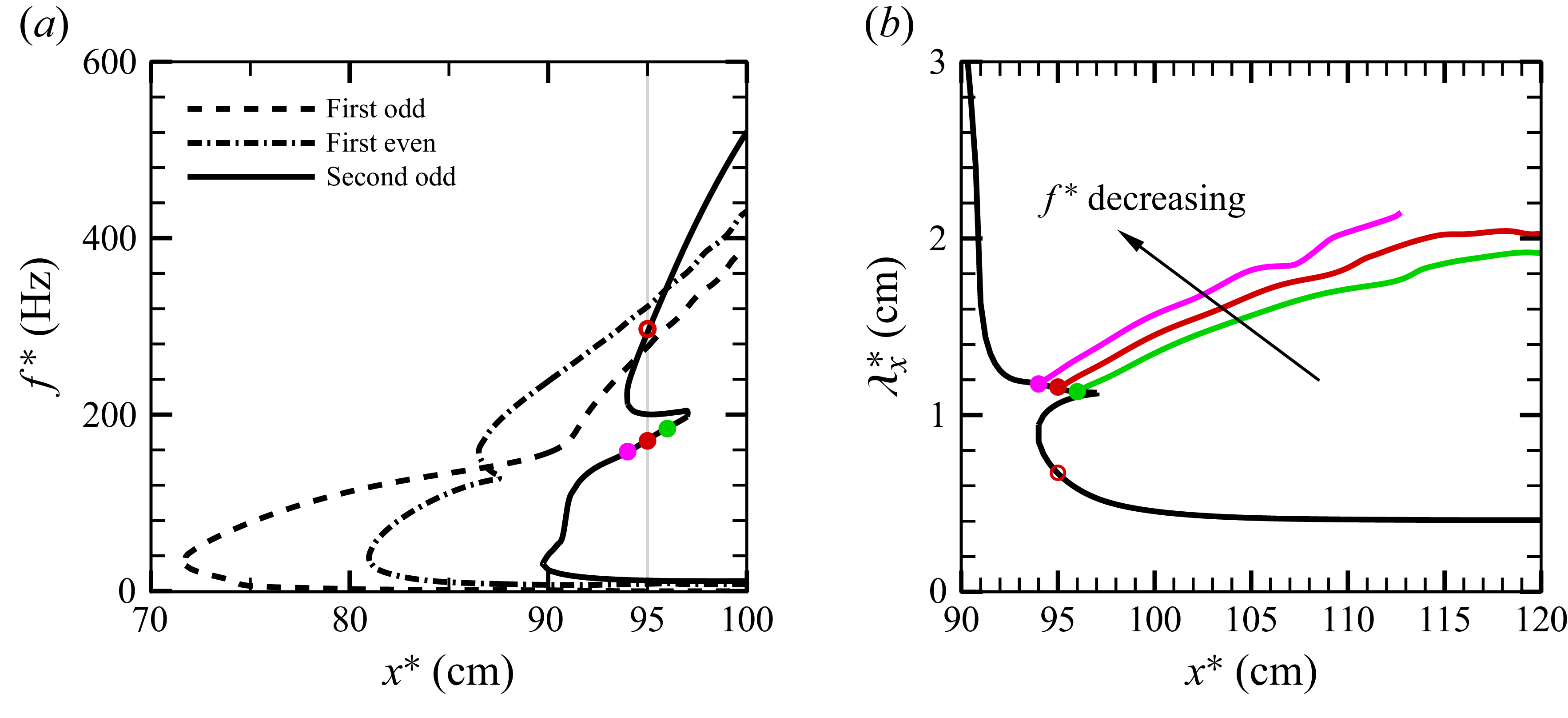
(a) Neutral curve in the $x^*$
–
$x^*$
– $f^*$
plane resulting from the secondary instability analysis. The filled circles are the linear critical points used in the PCS computations in panel (b). The open circle corresponds to the analysis in figure 6(b). (b) Local wavelength of the finite-amplitude wave obtained using the PCS method (the magenta, red and green lines correspond to
$f^*$
plane resulting from the secondary instability analysis. The filled circles are the linear critical points used in the PCS computations in panel (b). The open circle corresponds to the analysis in figure 6(b). (b) Local wavelength of the finite-amplitude wave obtained using the PCS method (the magenta, red and green lines correspond to $f^* = 157$
, 170 and 185 Hz, respectively). The black line shows the secondary instability analysis results for the second odd mode.
$f^* = 157$
, 170 and 185 Hz, respectively). The black line shows the secondary instability analysis results for the second odd mode.

To obtain the PCS result (red lines in figure 1), the secondary instability of the Görtler vortex must first be analysed. As reported in the previous studies, the instability exhibits three modes: the first odd, the first even and the second odd modes (see figures 19 and 21 of Xu et al. Reference Xu, Zhang and Wu2017, for example). Figure 2(a) shows the neutral curve obtained from our eigenvalue analysis. At each $x^*$
, we computed the values of
$x^*$
, we computed the values of $\alpha$
and
$\alpha$
and $c$
that yield neutrality (hereafter referred to as the linear critical point), and plotted the corresponding frequency
$c$
that yield neutrality (hereafter referred to as the linear critical point), and plotted the corresponding frequency $f^*=( { U^*_{\infty }}/{2\pi \delta ^*})c\alpha$
Hz. The first odd, first even and second odd modes instability appear around
$f^*=( { U^*_{\infty }}/{2\pi \delta ^*})c\alpha$
Hz. The first odd, first even and second odd modes instability appear around $x^* = 70$
,
$x^* = 70$
, $80$
and
$80$
and $90$
cm, respectively. At
$90$
cm, respectively. At $x^* = 95$
cm, several linear critical points exist. One of these, corresponding to the second odd mode and marked by the red circle, has a frequency comparable to the 130 Hz observed by SB87 at
$x^* = 95$
cm, several linear critical points exist. One of these, corresponding to the second odd mode and marked by the red circle, has a frequency comparable to the 130 Hz observed by SB87 at $x^* = 100$
cm. Hence, the vicinity of this point provides a suitable starting location for the PCS spatial marching including the finite-amplitude waves.
$x^* = 100$
cm. Hence, the vicinity of this point provides a suitable starting location for the PCS spatial marching including the finite-amplitude waves.
The magenta, red and green curves in figure 2(b) show the PCS results obtained using the frequencies $f^* = 157$
, 170 and 185 Hz, respectively. The corresponding linear critical points are approximately at
$f^* = 157$
, 170 and 185 Hz, respectively. The corresponding linear critical points are approximately at $x^* = 94$
, 95 and 96 cm. Recall that in the PCS calculations, we must fix
$x^* = 94$
, 95 and 96 cm. Recall that in the PCS calculations, we must fix $\varOmega = ( {2\pi \delta ^*}/{ U^*_{\infty }})f^*$
and this condition yields the local wavenumber
$\varOmega = ( {2\pi \delta ^*}/{ U^*_{\infty }})f^*$
and this condition yields the local wavenumber $\alpha$
at each streamwise location. The corresponding local wavelengths
$\alpha$
at each streamwise location. The corresponding local wavelengths $\lambda _x^* = 2\pi \delta ^*/\alpha$
shown in figure 2(b) are comparable to the 2–2.5 cm reported in SB87. All subsequent calculations in this section and the results shown in figure 1 use the PCS solution beginning at
$\lambda _x^* = 2\pi \delta ^*/\alpha$
shown in figure 2(b) are comparable to the 2–2.5 cm reported in SB87. All subsequent calculations in this section and the results shown in figure 1 use the PCS solution beginning at $x^* \approx 95$
cm (the red line,
$x^* \approx 95$
cm (the red line, $f^*=170$
Hz), unless otherwise stated. Computations starting too far upstream terminate before reaching
$f^*=170$
Hz), unless otherwise stated. Computations starting too far upstream terminate before reaching $x^* = 120$
cm, as indicated by the magenta line. Conversely, if the starting point is chosen too far downstream, the linear critical point corresponding to the relevant frequency disappears (see figure 2
a).
$x^* = 120$
cm, as indicated by the magenta line. Conversely, if the starting point is chosen too far downstream, the linear critical point corresponding to the relevant frequency disappears (see figure 2
a).
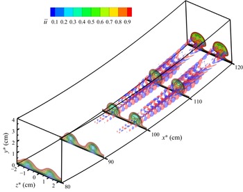
A snapshot of the flow field computed using the PCS. The colourmap at the selected streamwise positions shows the steady streak field $\overline {u}$
. Red/blue isosurfaces are 20 % maximum/minimum of the streamwise vorticity of the wave component,
$\overline {u}$
. Red/blue isosurfaces are 20 % maximum/minimum of the streamwise vorticity of the wave component, $\partial _y\tilde {w}-\partial _z \tilde {v}$
.
$\partial _y\tilde {w}-\partial _z \tilde {v}$
.

Figure 3 illustrates the flow field obtained from the PCS computation. Recall that in the decomposition (2.2), the roll-streak part $\overline {\boldsymbol{u}}$
is stationary, while the wave field
$\overline {\boldsymbol{u}}$
is stationary, while the wave field $\tilde {\boldsymbol{u}}$
is time-periodic with period
$\tilde {\boldsymbol{u}}$
is time-periodic with period $2\pi /\varOmega$
. The colourmap of
$2\pi /\varOmega$
. The colourmap of $\overline {u}$
depicts the development of the Görtler vortices, which nonlinearly interact with the finite-amplitude waves represented by the isosurfaces.
$\overline {u}$
depicts the development of the Görtler vortices, which nonlinearly interact with the finite-amplitude waves represented by the isosurfaces.
Flow field at $x^*=100$
cm: (a) BRE; (b) PCS; (c) experimental results from figures 11 and 16 of SB87. The black lines show contours of
$x^*=100$
cm: (a) BRE; (b) PCS; (c) experimental results from figures 11 and 16 of SB87. The black lines show contours of $\overline {u}$
at
$\overline {u}$
at $0.1,0.2,\ldots ,0.9$
, with the thick line indicating 0.8. The red lines are contours of
$0.1,0.2,\ldots ,0.9$
, with the thick line indicating 0.8. The red lines are contours of $\tilde {u}_{\textit{rms}}=0.01,0.02$
and 0.03, with the thick line highlighting 0.02.
$\tilde {u}_{\textit{rms}}=0.01,0.02$
and 0.03, with the thick line highlighting 0.02.

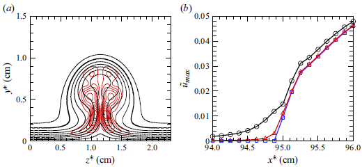
The black contours in figures 4(a) and 4(b) compare the BRE and PCS results for $\overline {u}$
at
$\overline {u}$
at $x = 100$
cm. The interaction between the vortex and the wave reduces the displacement thickness at the peak of the mushroom vortices, as seen in figure 1. Figure 4(a) presents the experimental results from SB87. The red contours in this figure, representing the root-mean-square velocity of the wave field
$x = 100$
cm. The interaction between the vortex and the wave reduces the displacement thickness at the peak of the mushroom vortices, as seen in figure 1. Figure 4(a) presents the experimental results from SB87. The red contours in this figure, representing the root-mean-square velocity of the wave field
 \begin{eqnarray} \tilde {u}_{\textit{rms}}(X,y,z)=\sqrt {\frac {1}{2\pi }\int ^{2\pi }_0\tilde {u}^2 \,{\rm d}\theta }, \end{eqnarray}
exhibit two peaks indicated by the arrows. The structures of peaks 1 and 2 resemble the first and second odd modes of the secondary instability, respectively (Xu et al. Reference Xu, Zhang and Wu2017). As expected, $\tilde {u}_{\textit{rms}}$
of the PCS result, continued from the second odd modes and shown in panel (b), closely resembles peak 2.
$\tilde {u}_{\textit{rms}}$
of the PCS result, continued from the second odd modes and shown in panel (b), closely resembles peak 2.
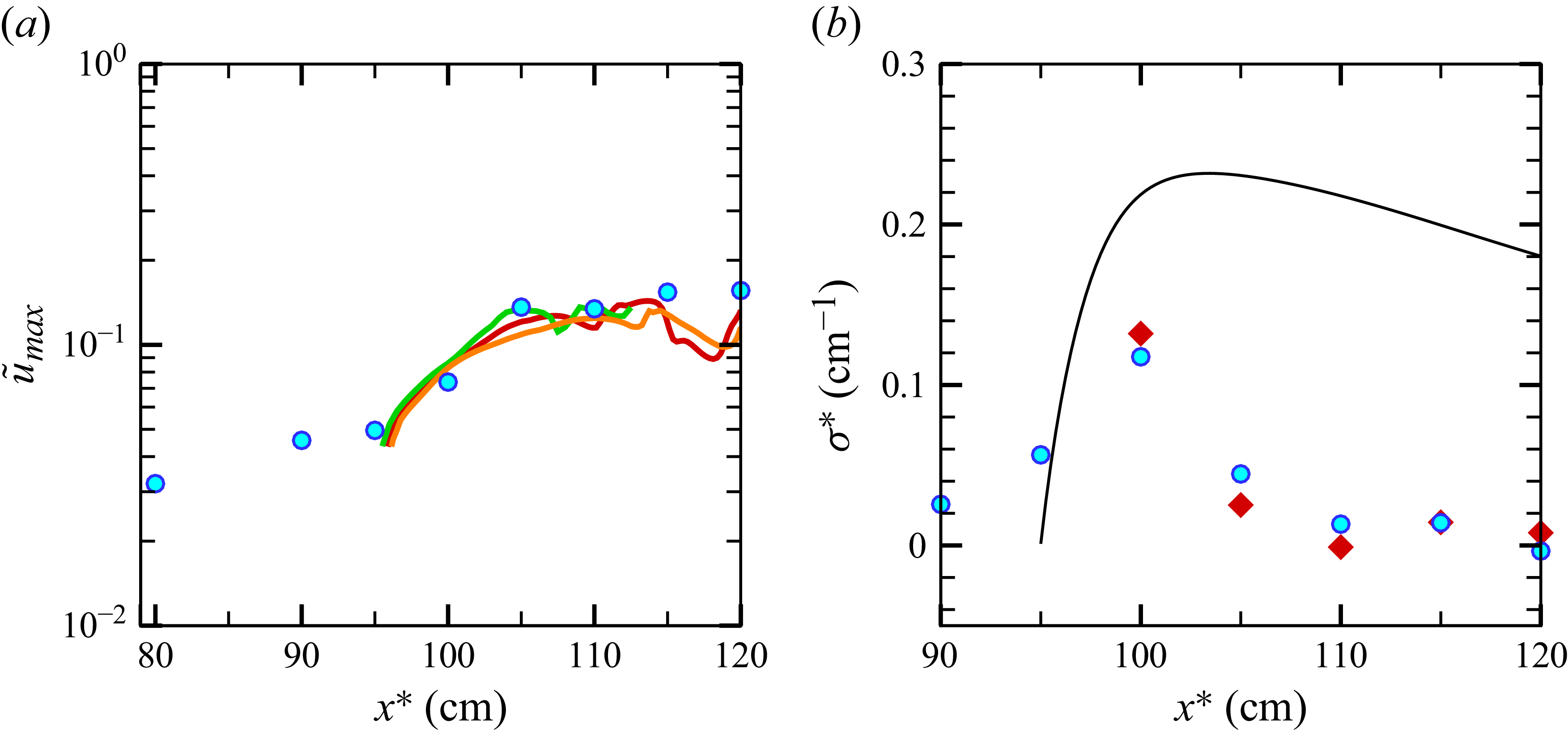
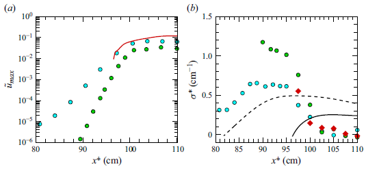
Downstream growth of the wave amplitude. (a) Amplitude of the wave field. Circles denote the experimental results taken from figure 17 in SB87. Lines are the PCS results shown in figure 2(b). (b) Growth rate $\sigma ^*=\sigma /L^*$
, where
$\sigma ^*=\sigma /L^*$
, where $\sigma (X)=( {1}/{\tilde {u}_{\textit{max}}})( {{\rm d} \tilde {u}_{\textit{max}}}/{{\rm d}X})$
. For a fair comparison, finite-difference approximations are applied to both the experimental (circles) and PCS (diamonds) results. The line shows the growth rate of the second odd mode predicted by the secondary instability analysis. Both computational results are for
$\sigma (X)=( {1}/{\tilde {u}_{\textit{max}}})( {{\rm d} \tilde {u}_{\textit{max}}}/{{\rm d}X})$
. For a fair comparison, finite-difference approximations are applied to both the experimental (circles) and PCS (diamonds) results. The line shows the growth rate of the second odd mode predicted by the secondary instability analysis. Both computational results are for $f^*=170$
Hz.
$f^*=170$
Hz.

SB87 noted that peak 1 emerges first, followed by the development of peak 2 for $x^*\geqslant 90$
cm, consistent with figure 2(a). Although peak 2 was less dominant at
$x^*\geqslant 90$
cm, consistent with figure 2(a). Although peak 2 was less dominant at $x^*=100$
cm in figure 4(c), it ultimately attained the highest amplitude in the experiments. The downstream growth of this peak can be quantified by the wave amplitude
$x^*=100$
cm in figure 4(c), it ultimately attained the highest amplitude in the experiments. The downstream growth of this peak can be quantified by the wave amplitude $\tilde {u}_{\textit{max}}(X)=\max _{y,z}\tilde {u}_{\textit{rms}}$
. As figure 5(a) indicates, the amplitude obtained by PCS agrees very well with the experimental results of SB87.
$\tilde {u}_{\textit{max}}(X)=\max _{y,z}\tilde {u}_{\textit{rms}}$
. As figure 5(a) indicates, the amplitude obtained by PCS agrees very well with the experimental results of SB87.
The experiments of SB87 strongly suggest that both of the two odd modes participate in the nonlinear interaction simultaneously. While it is possible to incorporate such multiple finite-amplitude waves in the PCS, this lies beyond the scope of the present work.
Yu & Liu (Reference Yu and Liu1994) attributed the seemingly linear growth around $x^* = 100$
cm shown in figure 5(a) to secondary instability. However, as shown in figure 5(b), the dimensional growth rate predicted by the secondary instability analysis (
$x^* = 100$
cm shown in figure 5(a) to secondary instability. However, as shown in figure 5(b), the dimensional growth rate predicted by the secondary instability analysis ( $\sigma ^* = -\Im (\alpha )/\delta ^*$
, indicated by the line) tends to be significantly larger than that observed experimentally; a similar conclusion was reached by Xu et al. (Reference Xu, Zhang and Wu2017). On the other hand, the PCS results are much closer to the experimental observations (red diamonds). The corresponding values of
$\sigma ^* = -\Im (\alpha )/\delta ^*$
, indicated by the line) tends to be significantly larger than that observed experimentally; a similar conclusion was reached by Xu et al. (Reference Xu, Zhang and Wu2017). On the other hand, the PCS results are much closer to the experimental observations (red diamonds). The corresponding values of $\sigma ^*$
are computed from the spatial evolution of the wave amplitude
$\sigma ^*$
are computed from the spatial evolution of the wave amplitude $\tilde {u}_{\textit{max}}(X)$
defined earlier; see the figure caption also. The physical roles of PCS and secondary instabilities in Navier–Stokes computations will be discussed in § 4.
$\tilde {u}_{\textit{max}}(X)$
defined earlier; see the figure caption also. The physical roles of PCS and secondary instabilities in Navier–Stokes computations will be discussed in § 4.
PCS results for various Reynolds numbers. Panels (a) and (c) show the same computational results for the wave amplitude and the displacement thickness at the peak vortex location, respectively. The computations are performed from the linear critical point $x^*\approx 95$
cm using
$x^*\approx 95$
cm using $\varOmega \approx 0.1$
(
$\varOmega \approx 0.1$
( $\varOmega =0.1080,0.1216$
and
$\varOmega =0.1080,0.1216$
and $0.1262$
for
$0.1262$
for $\textit{Re}=15\,625, 31\,250$
and
$\textit{Re}=15\,625, 31\,250$
and $40\,000$
, respectively). Panels (b) and (d) present results corresponding to panels (a) and (c), respectively, but at a higher frequency
$40\,000$
, respectively). Panels (b) and (d) present results corresponding to panels (a) and (c), respectively, but at a higher frequency $\varOmega \approx 0.2$
(
$\varOmega \approx 0.2$
( $\varOmega =0.2079,0.2126,0.2180$
and
$\varOmega =0.2079,0.2126,0.2180$
and $0.2269$
for
$0.2269$
for $\textit{Re}=31\,250, 40\,000, 50\,000$
and
$\textit{Re}=31\,250, 40\,000, 50\,000$
and $60\,000$
, respectively).
$60\,000$
, respectively).

Finally, we examine the dependence of the computational results on the Reynolds number. The PCS system retains not only the leading order terms, but also higher order terms. Therefore, studying whether the PCS solution attains asymptotic convergence is necessary. The red line in figure 6(a) shows the same result as the $f^* = 170$
Hz line in figure 5(a). In addition, we include results for two different
$f^* = 170$
Hz line in figure 5(a). In addition, we include results for two different $\textit{Re}$
, adjusting
$\textit{Re}$
, adjusting $\varOmega$
so that the neutral point occurs at approximately
$\varOmega$
so that the neutral point occurs at approximately $x^*=95$
cm. According to the VWI theory (Hall & Smith Reference Hall and Smith1991; Hall & Sherwin Reference Hall and Sherwin2010), the wave amplitude acquires a larger magnitude within the critical layer by a factor of
$x^*=95$
cm. According to the VWI theory (Hall & Smith Reference Hall and Smith1991; Hall & Sherwin Reference Hall and Sherwin2010), the wave amplitude acquires a larger magnitude within the critical layer by a factor of $\epsilon ^{-1}$
so that
$\epsilon ^{-1}$
so that $\tilde {u}_{\textit{max}}$
scales as
$\tilde {u}_{\textit{max}}$
scales as $\epsilon ^{-1}\times \epsilon ^{1/2}R_{\delta }^{-1}=R_{\delta }^{-5/6}$
. After rescaling the computationally obtained
$\epsilon ^{-1}\times \epsilon ^{1/2}R_{\delta }^{-1}=R_{\delta }^{-5/6}$
. After rescaling the computationally obtained $\tilde {u}_{\textit{max}}$
by
$\tilde {u}_{\textit{max}}$
by $R_{\delta }^{5/6}$
, the two highest
$R_{\delta }^{5/6}$
, the two highest $\textit{Re}$
results lie close each other, at least up to approximately
$\textit{Re}$
results lie close each other, at least up to approximately $x^*=110$
cm, which is the range of interest in this study. Figure 6(c) shows a similar comparison, but for the displacement thickness at the peaks of the Görtler vortices (the same format as figure 1). Again, a reasonably good level of convergence can be observed. We performed the same test using a higher frequency,
$x^*=110$
cm, which is the range of interest in this study. Figure 6(c) shows a similar comparison, but for the displacement thickness at the peaks of the Görtler vortices (the same format as figure 1). Again, a reasonably good level of convergence can be observed. We performed the same test using a higher frequency, $f^*\approx 280$
Hz, for which another critical point appears around
$f^*\approx 280$
Hz, for which another critical point appears around $x^*=95$
cm (open circle in figure 2
a). The results are shown in figures 6(b) and 6(d). This second test shows the asymptotic convergence more clearly, probably because in the first test, the neutral curve exhibits relatively complex behaviour at the onset of finite amplitude waves (see figure 2
a).
$x^*=95$
cm (open circle in figure 2
a). The results are shown in figures 6(b) and 6(d). This second test shows the asymptotic convergence more clearly, probably because in the first test, the neutral curve exhibits relatively complex behaviour at the onset of finite amplitude waves (see figure 2
a).
Hall (Reference Hall1988) showed that the residual in the BRE approximation is very small and is $O(R_{\delta }^{-2})$
relative to the leading order. However, in the PCS, we also need to take into account the asymptotic convergence of the wave part (2.8). This part has the same structure as the secondary instability equations, and its leading order part was recently solved by Deguchi (Reference Deguchi2019) for a model base flow and compared with finite Reynolds number results. Based on the results of Deguchi (Reference Deguchi2019), a Reynolds number of
$O(R_{\delta }^{-2})$
relative to the leading order. However, in the PCS, we also need to take into account the asymptotic convergence of the wave part (2.8). This part has the same structure as the secondary instability equations, and its leading order part was recently solved by Deguchi (Reference Deguchi2019) for a model base flow and compared with finite Reynolds number results. Based on the results of Deguchi (Reference Deguchi2019), a Reynolds number of $O(10^4)$
, defined using the characteristic length and velocity scales of the base flow, is sufficient to achieve good asymptotic convergence. In our computation, with a typical height of the Görtler vortices
$O(10^4)$
, defined using the characteristic length and velocity scales of the base flow, is sufficient to achieve good asymptotic convergence. In our computation, with a typical height of the Görtler vortices $d^*\approx 1$
cm (see figure 1), the effective local Reynolds number can be estimated as
$d^*\approx 1$
cm (see figure 1), the effective local Reynolds number can be estimated as $d^* U_{\infty }^*/\nu ^*\approx O(10^3)$
–
$d^* U_{\infty }^*/\nu ^*\approx O(10^3)$
– $O(10^4)$
, which supports the observations in figure 6.
$O(10^4)$
, which supports the observations in figure 6.
Note that in figure 6, the horizontal axis is $x^*=L^*X$
, where
$x^*=L^*X$
, where $L^*=10$
cm is used for dimensionalisation. Convergence of the wave amplitude/roll-streaks in this coordinate thus implies convergence in the
$L^*=10$
cm is used for dimensionalisation. Convergence of the wave amplitude/roll-streaks in this coordinate thus implies convergence in the $X$
coordinate. By contrast, the wavelength is scaled with
$X$
coordinate. By contrast, the wavelength is scaled with $\delta ^*=\textit{Re}^{-1/2}L^*$
; thus, increasing
$\delta ^*=\textit{Re}^{-1/2}L^*$
; thus, increasing $\textit{Re}$
leads to a shorter wavelength in the
$\textit{Re}$
leads to a shorter wavelength in the $x^*$
coordinate. For example, in figure 6(b), the typical wavelength is 0.7–1.2 cm for
$x^*$
coordinate. For example, in figure 6(b), the typical wavelength is 0.7–1.2 cm for $\textit{Re}=31\,250$
and decreases to 0.4–0.7 cm for
$\textit{Re}=31\,250$
and decreases to 0.4–0.7 cm for $\textit{Re}=60\,000$
.
$\textit{Re}=60\,000$
.
4. Discussion
This paper presents a theoretical and computational study of the development of finite-amplitude waves on Görtler vortices in a boundary layer over a concave wall. Conventionally, the evolution of such waves is explained by tracing the spatial growth of dominant secondary instability modes. In contrast, the PCS determine the wave amplitude by requiring the waves to be self-sustained neutral modes: the Reynolds stresses arising from the interaction of the travelling waves modify rolls and streaks, and the resulting streaks, in turn, render the waves neutral.
The growth rate $\sigma (X)=( {1}/{\tilde {u}_{\textit{max}}})( {{\rm d} \tilde {u}_{\textit{max}}}/{{\rm d}X})$
computed by the slow-scale variation of the wave amplitude
$\sigma (X)=( {1}/{\tilde {u}_{\textit{max}}})( {{\rm d} \tilde {u}_{\textit{max}}}/{{\rm d}X})$
computed by the slow-scale variation of the wave amplitude $\tilde {u}_{\textit{max}}$
agrees better with the SB87 experimental results than the prediction from the secondary instability analysis (figure 5). Moreover, as shown in figure 1, the PCS method successfully reproduces the displacement thickness observed in the experiments up to
$\tilde {u}_{\textit{max}}$
agrees better with the SB87 experimental results than the prediction from the secondary instability analysis (figure 5). Moreover, as shown in figure 1, the PCS method successfully reproduces the displacement thickness observed in the experiments up to $x^*$
= 110 cm, where vortex breakdown to turbulence is reported. These results are intriguing, as they show that the PCS approach, which intrinsically incorporates an extension of exact coherent structures, can yield meaningful results for non-parallel flows.
$x^*$
= 110 cm, where vortex breakdown to turbulence is reported. These results are intriguing, as they show that the PCS approach, which intrinsically incorporates an extension of exact coherent structures, can yield meaningful results for non-parallel flows.
While the PCS predictions perform well, some caution is nevertheless required when interpreting our results. In particular, our results are generated using a rather arbitrary initial condition, chosen primarily for simplicity. Görtler vortices can also be generated by vortical perturbations passively advected from upstream in the oncoming uniform flow (Wu, Zhao & Luo Reference Wu, Zhao and Luo2011; Xu et al. Reference Xu, Zhang and Wu2017) or coherent structures self-sustained in free stream (Deguchi & Hall Reference Deguchi and Hall2014a , Reference Deguchi and Hall2017; Dempsey, Hall & Deguchi Reference Dempsey, Hall and Deguchi2017). Using those more realistic and complex conditions may lead to improved predictions.
In the PCS marching, we used a small artificial forcing (see Appendix A) near the neutral point of the secondary instability analysis. This forcing is introduced merely as a means to generate finite-amplitude states and, as long as its amplitude is small, the downstream PCS results are unaffected by the distribution of the forcing. However, in experiments, the external perturbations are not always small; in fact, the experiments of SB87 appear to be exposed to non-negligible finite-amplitude free stream turbulence. Therefore, it is of interest to replace the forcing in the PCS with a physically meaningful, large-amplitude signal. Several external effects for inducing wave-like activities have been proposed in the shear flow transition community. These include unsteady free stream vortical disturbances in boundary-layer flows (Zhang, Dong & Zhang Reference Zhang, Dong and Zhang2018), as well as oscillatory pressure gradients and sinusoidal wavy walls in plane channel flows (Luo & Wu Reference Luo and Wu2004).
The PCS approach requires the value of $\varOmega$
to be prescribed. In the experiments, the frequency of the wave-like activity appears to be set by an external perturbation, the nature of which is not described in SB87. We therefore estimate
$\varOmega$
to be prescribed. In the experiments, the frequency of the wave-like activity appears to be set by an external perturbation, the nature of which is not described in SB87. We therefore estimate $\varOmega$
from the experiments. That said, the range of admissible frequencies in the PCS computation is not entirely free: a corresponding neutral point must exist in the secondary instability analysis and the spatial integration must proceed stably.
$\varOmega$
from the experiments. That said, the range of admissible frequencies in the PCS computation is not entirely free: a corresponding neutral point must exist in the secondary instability analysis and the spatial integration must proceed stably.
We also remark that the conventional transition route via the modally unstable modes certainly play a major role in boundary layer transitions and should not be dismissed (see the review papers by Reed, Saric & Arnal Reference Reed, Saric and Arnal1996 and Saric, Reed & White Reference Saric, Reed and White2003 for the primal instability in flat-plate or swept-wing boundary layers, and Li et al. Reference Li, Choudhari and Paredes2022 and references therein for the secondary instability in the Görtler vortex problem). The absence of this behaviour in the SB87 experiment can be explained by two factors: (i) the experimental set-up is subjected to relatively large oncoming disturbances; and (ii) in the Görtler vortex problem, even very small wave amplitudes can significantly affect the streaks.
The need to consider factor (i) is apparent from figure 5(a), where $\tilde {u}_{\textit{max}}$
is not small, being of order
$\tilde {u}_{\textit{max}}$
is not small, being of order $O(10^{-2})$
, even upstream of the transition point. The external perturbation level can be more easily controlled in DNS and Souza (Reference Souza2017) reported a case in which the upstream
$O(10^{-2})$
, even upstream of the transition point. The external perturbation level can be more easily controlled in DNS and Souza (Reference Souza2017) reported a case in which the upstream $\tilde {u}_{\textit{max}}$
is
$\tilde {u}_{\textit{max}}$
is $O(10^{-5})$
. Using the parameters from this simulation, we confirmed that the secondary instability analysis reasonably explains the initial growth of wave perturbations (see Appendix B).
$O(10^{-5})$
. Using the parameters from this simulation, we confirmed that the secondary instability analysis reasonably explains the initial growth of wave perturbations (see Appendix B).
Factor (ii) can be understood by a feature of VWI theory that even very small wave amplitudes significantly affect the streaks. As is well known, VWI inherently contains the self-sustained process (Hamilton et al. Reference Hamilton, Kim and Waleffe1995; Waleffe Reference Waleffe1997), in which the waves drive the rolls through the Reynolds stress, the rolls modify the streaks via the lift-up mechanism and the resulting modulation of the streaks then influences the waves. Among these, the lift-up mechanism is the key for amplifying small perturbations and it can exist only for three-dimensional perturbations. VWI is also relevant to bypass transition and it is noteworthy that the scenario described here may be applicable.
The previous argument implies that exponentially growing perturbations rapidly violate the small-amplitude assumption underlying linear analysis and thus persist only over short spatiotemporal scales. From a physical perspective, the locally neutral solution may therefore be the one that tends to survive the longest. Indeed, a closer look at the analysis of § 2.1 shows that local neutrality is an essential requirement for constructing the rational asymptotic theory; without it, the Reynolds stress would depend on the fast variable $\theta$
, contradicting the assumption that the roll-streak field
$\theta$
, contradicting the assumption that the roll-streak field $\overline {\boldsymbol{u}}$
is independent of
$\overline {\boldsymbol{u}}$
is independent of $\theta$
. The consistency with the VWI is precisely what enables the PCS method to combine the efficiency of the spatial marching approach with the robustness of exact coherent-structure computations.
$\theta$
. The consistency with the VWI is precisely what enables the PCS method to combine the efficiency of the spatial marching approach with the robustness of exact coherent-structure computations.
In conclusion, the PCS describes the saturated stage of the finite amplitude waves, while the earlier substantial amplification phase is not captured. On the other hand, only when the wave amplitude is extremely small, the most amplified mode in the linear stability analysis dominates the initial transition process. Thus, the two methods are complementary.
Finally, we note that the significance of our results also lies in the long-awaited achievement of the first numerical computation of VWI in spatially growing boundary-layer flows, originally formulated by Hall & Smith (Reference Hall and Smith1991). The solution obtained in § 3 approximates a time-periodic exact coherent structure, which is very likely unstable. It is noteworthy that, in the parallel flow research community, such unstable periodic orbits are now recognised as fundamental building blocks for understanding turbulence from a dynamical systems theory perspective (Kawahara, Uhlmann & van Veen Reference Kawahara, Uhlmann and van Veen2012). We expect that a similar approach will, in the future, become increasingly popular for realistic flows with non-parallel effects, where the efficient computational strategy of the PCS will play a key role.
Acknowledgements
This research was supported by the Australian Research Council Discovery Project DP230102188.
Declaration of interests
The authors report no conflicts of interest.
Appendix A. Generation of finite amplitude waves by external forcing
Here, we elaborate on the forcing approach for obtaining a finite amplitude wave solution in the PCS system. All the results presented here are obtained for $f^*=170$
Hz. For this frequency, the secondary instability analysis identifies a zero growth rate for the second odd mode at
$f^*=170$
Hz. For this frequency, the secondary instability analysis identifies a zero growth rate for the second odd mode at $x^* \approx 94.88$
cm. Figure 7(a) shows the corresponding neutral eigenfunction, normalised so that
$x^* \approx 94.88$
cm. Figure 7(a) shows the corresponding neutral eigenfunction, normalised so that $\tilde {u}_{\textit{max}}=1$
. We denote this normalised function by
$\tilde {u}_{\textit{max}}=1$
. We denote this normalised function by $[\tilde {\boldsymbol{u}}_c,\tilde {p}_c]$
.
$[\tilde {\boldsymbol{u}}_c,\tilde {p}_c]$
.
(a) Analysis near the linear critical point of the second odd mode at $f^*=170$
Hz. The red lines are contours of
$f^*=170$
Hz. The red lines are contours of $|\hat u|$
associated with the neutral eigenfunction found by the secondary instability analysis. The black lines denote the contours of the base flow
$|\hat u|$
associated with the neutral eigenfunction found by the secondary instability analysis. The black lines denote the contours of the base flow $\bar {u}$
at the linear critical point (the same format as figure 4). (b) PCS computation near the linear critical point
$\bar {u}$
at the linear critical point (the same format as figure 4). (b) PCS computation near the linear critical point $x^*=94.88$
cm. The external forcing term is added to (2.8a
). The blue, red and black lines correspond to
$x^*=94.88$
cm. The external forcing term is added to (2.8a
). The blue, red and black lines correspond to $A=2\times 10^{-5}$
,
$A=2\times 10^{-5}$
, $2\times 10^{-4}$
and
$2\times 10^{-4}$
and $2\times 10^{-3}$
, respectively.
$2\times 10^{-3}$
, respectively.

Now, let us consider the spatial marching step near the neutral point. In the BRE computation, the Newton–Raphson method yields the updated field $[\overline {\boldsymbol{u}},\overline {p}]$
. This is, of course, the solution of the PCS system with no wave component. We then substitute
$[\overline {\boldsymbol{u}},\overline {p}]$
. This is, of course, the solution of the PCS system with no wave component. We then substitute $[A\tilde {\boldsymbol{u}}_c,A\tilde {p}_c]$
with the prescribed finite amplitude
$[A\tilde {\boldsymbol{u}}_c,A\tilde {p}_c]$
with the prescribed finite amplitude $A$
; this introduces a small but non-zero residual. The residual in the wave momentum equation (2.8a
) is the external forcing term mentioned at the end of § 2. That is, the forcing enters (2.8a
) as an inhomogeneous term and is a function of
$A$
; this introduces a small but non-zero residual. The residual in the wave momentum equation (2.8a
) is the external forcing term mentioned at the end of § 2. That is, the forcing enters (2.8a
) as an inhomogeneous term and is a function of $A$
.
$A$
.
Figure 7(b) shows the spatial marching result near the neutral point, where the forcing is switched on at $x^*=94$
cm. As shown by the blue curve, even a very small value of
$x^*=94$
cm. As shown by the blue curve, even a very small value of $A=2\times 10^{-5}$
allows the finite amplitude wave solution branch to be captured. The frequency of the PCS solution emanated from the neutral point matches that of the applied forcing. When the amplitude is increased to
$A=2\times 10^{-5}$
allows the finite amplitude wave solution branch to be captured. The frequency of the PCS solution emanated from the neutral point matches that of the applied forcing. When the amplitude is increased to $A=2\times 10^{-4}$
(red curve), the effect of the forcing becomes apparent in the vicinity of the neutral point. In dynamical system analysis, the region near a bifurcation point is often most sensitive to inhomogeneous terms. This phenomenon is known as imperfect bifurcation, which we have exploited in our approach. The black curve corresponds to an even larger amplitude,
$A=2\times 10^{-4}$
(red curve), the effect of the forcing becomes apparent in the vicinity of the neutral point. In dynamical system analysis, the region near a bifurcation point is often most sensitive to inhomogeneous terms. This phenomenon is known as imperfect bifurcation, which we have exploited in our approach. The black curve corresponds to an even larger amplitude, $A=2\times 10^{-3}$
; at this forcing level, the small deviation from the blue curve persists downstream.
$A=2\times 10^{-3}$
; at this forcing level, the small deviation from the blue curve persists downstream.
We have tested several different transverse structures for the forcing and obtained qualitatively the same results; as long as the amplitude is small, the effect of the forcing does not appear downstream. In § 3, we use the result obtained with $A=2\times 10^{-5}$
in figure 6(b) and switch off the forcing at
$A=2\times 10^{-5}$
in figure 6(b) and switch off the forcing at $x^*=95.5$
cm.
$x^*=95.5$
cm.
Appendix B. Comparison with DNS
Figure 8 presents a comparison similar to that in figure 5, using the DNS of Souza (Reference Souza2017). In the DNS, the Görtler vortices are first generated by a steady disturbance generator and an unsteady perturbation is then introduced at $x^* \in [75.05,78.25]$
cm via a second disturbance generator. The second generator is driven by oscillatory blowing and suction on the wall, producing a wide range of frequencies (from 20 to 320 Hz). In figure 13 of Souza (Reference Souza2017), the downstream evolution of the wave amplitude for each frequency is recorded. Initially, low frequency modes near 120 Hz are excited around
$x^* \in [75.05,78.25]$
cm via a second disturbance generator. The second generator is driven by oscillatory blowing and suction on the wall, producing a wide range of frequencies (from 20 to 320 Hz). In figure 13 of Souza (Reference Souza2017), the downstream evolution of the wave amplitude for each frequency is recorded. Initially, low frequency modes near 120 Hz are excited around $x^*=80$
cm, followed by the higher frequency modes, such as those around 180 Hz. The green and blue circles in figure 8 are representative data from DNS.
$x^*=80$
cm, followed by the higher frequency modes, such as those around 180 Hz. The green and blue circles in figure 8 are representative data from DNS.
Comparison with DNS. (a) Amplitude of the wave field. Blue and green circles represent the DNS data reported by Souza (Reference Souza2017) for 120 and 180 Hz, respectively. The red line shows the PCS result for $f^*=180$
Hz. (b) Growth rate. The circles and diamonds are computed from the DNS and PCS data, respectively. The lines are the secondary instability analysis results. The dashed line is the first odd mode at 120 Hz; the solid line is the second odd mode at 180 Hz.
$f^*=180$
Hz. (b) Growth rate. The circles and diamonds are computed from the DNS and PCS data, respectively. The lines are the secondary instability analysis results. The dashed line is the first odd mode at 120 Hz; the solid line is the second odd mode at 180 Hz.

Souza (Reference Souza2017) used the spanwise period $\lambda ^*=1.8$
cm and the Reynolds number
$\lambda ^*=1.8$
cm and the Reynolds number $\textit{Re}=331\,24$
, which differ slightly from those used in § 3. Therefore, we produced the PCS results using these parameters as shown by the red line in figure 8(a). We used
$\textit{Re}=331\,24$
, which differ slightly from those used in § 3. Therefore, we produced the PCS results using these parameters as shown by the red line in figure 8(a). We used $f^*=180$
Hz, for which the linear critical point exists around
$f^*=180$
Hz, for which the linear critical point exists around $x^*=96$
cm. Since the forcing approach is used (see Appendix A), we show only the amplitude levels where the results are unaffected by the forcing. The red diamonds in figure 8(b) represent the growth rates calculated from PCS and show good agreement with the results from DNS when the wave amplitude is sufficiently large. Note that some discrepancy is expected, because the BRE computation uses rather arbitrary analytic initial condition as mentioned in § 2. Introduction of the steady disturbance generator used by Souza (Reference Souza2017) would require substantial modifications to the BRE code, which are beyond the scope of this paper.
$x^*=96$
cm. Since the forcing approach is used (see Appendix A), we show only the amplitude levels where the results are unaffected by the forcing. The red diamonds in figure 8(b) represent the growth rates calculated from PCS and show good agreement with the results from DNS when the wave amplitude is sufficiently large. Note that some discrepancy is expected, because the BRE computation uses rather arbitrary analytic initial condition as mentioned in § 2. Introduction of the steady disturbance generator used by Souza (Reference Souza2017) would require substantial modifications to the BRE code, which are beyond the scope of this paper.
We also performed secondary instability analyses and confirmed that the results are similar to those shown in figure 2(a). The first odd mode appears initially and its growth rate at 120 Hz is obtained as the black dashed line in figure 8(b). This result appears reasonably close to the DNS results when the wave amplitude remains very small. We also examined the second odd mode at 180 Hz (black solid line), but it does not yield particularly meaningful results.
In our survey, we found only a few references for the validation of secondary instability analysis: Li et al. (Reference Li, Choudhari, Chang, Greene and Wu2010) compared it with the results by the nonlinear parabolised equations and Chen, Huang & Lee (Reference Chen, Huang and Lee2019) compared it with DNS. In both cases, agreement comparable to ours was observed. If linear parabolised stability equations are used, the incorporation of non-parallel effects significantly improves agreement with DNS (see Song, Zhao & Huang Reference Song, Zhao and Huang2020).












 Open access

