


1. Introduction
The study of thermoacoustic instabilities has attracted considerable interest in the past (Rayleigh Reference Rayleigh1878; Markstein Reference Markstein1951; Veiga-López et al. Reference Veiga-López, Martínez-Ruiz, Kuznetsov and Sánchez-Sanz2020), with a vast range of approaches and efforts to provide a better understanding of the phenomenon (Pelcé & Rochwerger Reference Pelcé and Rochwerger1992; Assier & Wu Reference Assier and Wu2014). Besides the physical interest, its thermochemical character is tightly linked to the acoustics and flow dynamics, resulting in a very complex process. Furthermore, engineers engaged in the development of thermal power technologies are keenly interested in this phenomenon, as it has the potential to cause significant deterioration in performance and severe structural damage to combustion chambers. Thermoacoustic instability issues frequently arise in industrial combustion systems, including burners (Morgans, Goh & Dahan Reference Morgans, Goh and Dahan2013), boilers, combustion furnaces (Altay et al. Reference Altay, Park, Wu, Wee, Annaswamy and Ghoniem2009) and in aerospace propulsion systems (Xia et al. Reference Xia, Laera, Jones and Morgans2019; Hashimoto et al. Reference Hashimoto, Shibuya, Gotoda, Ohmichi and Matsuyama2019).
Continuous efforts are typically oriented towards the effects of chamber configuration (Srikanth et al. Reference Srikanth, Sahay, Pawar, Manoj and Sujith2022), new visualisation techniques (Choudhury, Syam & Joarder Reference Choudhury, Syam and Joarder2023), material properties such as heat-transfer (Mejia et al. Reference Mejia, Selle, Bazile and Poinsot2015) or elastic dissipation mechanisms (Rubio-Rubio et al. Reference Rubio-Rubio, Veiga-López, Martínez-Ruiz, Fernández-Tarrazo and Sánchez-Sanz2023) and mixture properties (Ananthakrishnan et al. Reference Ananthakrishnan, Choudhury, Syam, Joarder, Krishna Mohan, Dutta, Subudhi and Singh2024). In fact, a wide variety of control mechanisms are available for the dissipation of thermoacoustic waves, which are typically classified into passive and active categories. Passive control mechanisms entail the introduction of additional acoustic losses or damping into combustion chambers with the objective of mitigating the effects of acoustic disturbances. Typical examples of such dissipators include Helmholtz resonators (Yang, Wang & Zhu Reference Yang, Wang and Zhu2014; Zhang et al. Reference Zhang, Zhao, Han, Wang and Li2015; Cai & Mak Reference Cai and Mak2018) and expansion chambers or cavities (Jo, Choi & Kim Reference Jo, Choi and Kim2019). The primary limitation of these passive control methods is that they are designed to mitigate a specific set of frequencies, which restricts the method’s range of applicability and efficiency when a wide range of frequencies is present. Conversely, active control mechanisms employ pressure monitoring systems and sequential dynamic actuators, such as valves and loudspeakers, to interrupt the coupling phenomena associated with thermoacoustic waves (Li et al. Reference Li, Li, Tang, Yang, Fu, Clarke, Jin, Ji and Zhao2016). One of the primary limitations of active controllers is the requirement for rapid response, especially in high-frequency regimes. Furthermore, these control mechanisms depend on electronic devices to prevent instabilities, which can introduce further complexity and potential points of failure.
In this paper, we explore the fundamental effects of enhanced viscous dissipation on a thermoacoustically unstable flow via porous structures. The placement of these plugs inside the combustion chamber produces variations in the natural acoustic modes and additional energy dissipation, which are here characterised in the presence of simple and well-controlled experimental set-ups. To this end, different types of porous structures are designed and selected to tune their properties and help explain the variations of such mitigation behaviours for the flame propagating in thin channels. A key safety concern motivating this work is the propagation of flames in combustion set-ups where the excitation of instabilities can lead to hazardous conditions. Furthermore, from a fundamental perspective, the acoustic response of a propagating flame is thought to influence the formation of complex flame structures, such as tulip flames (Xiao, Houim & Oran Reference Xiao, Houim and Oran2015). In our experiments, the flame front undergoes a rapid evolution driven by changes in the flame surface area and cellular structures (Pelcé & Rochwerger Reference Pelcé and Rochwerger1992). Although a simpler configuration, such as a Rijke tube, with a fixed heat-release location could be used, it would not capture these intricate interactions between flame dynamics and acoustics, and would be subject to a specific acoustic frequency prescribed by the tube length and the heat-release position. Therefore, a propagating flame tube is used here to serve as a dynamic benchmark of acoustic-mitigation testing in a wide range of frequencies and provides, as a side product, further valuable information for their application in combustion chambers and accidental reactive events.
In recent years, advancements in additive manufacturing techniques have enabled the design and fabrication of components that would be unfeasible using traditional methods (Braun & Iváñez Reference Braun and Iváñez2020; Braun, Iváñez & Aranda-Ruiz Reference Braun, Iváñez and Aranda-Ruiz2020). One such example is the fabrication of metamaterials based on lattice structures (Liao et al. Reference Liao, Luan, Wang, Liu, Yao and Fu2021; Gao et al. Reference Gao, Zhang, Deng, Guo, Cheng and Hou2022). In this study, we have employed the advantages of this technique to design porous plugs that have been manufactured using low-force stereolithography. The efficacy of these devices has been evaluated in relation to different pore sizes and their positions within the tube. Furthermore, experimental tests were conducted to determine the characteristic permeability of the porous structures and provide a theoretical representation of the effect at hand.
The advantage of incorporating porous pieces in burners, in comparison with alternative methods of instability control, is their wide robustness and simplicity, as they are not limited to dissipating waves within a specific frequency range, nor do they require the use of additional electronic devices. In addition, 3-D printing technology allows their easy adaptation to applications with different geometries. The experimental results show the effectiveness of this passive control mechanism for thermoacoustic instabilities in such tubes and the optimal design parameters and placement that enhance their performance. They warn, as well, about the alteration produced in the system’s eigenfrequencies upon the introduction of porous plugs.
Moreover, a one-dimensional theoretical model, based on the formulation presented by Flores-Montoya et al. (Reference Flores-Montoya, Muntean, Sánchez-Sanz and Martínez-Ruiz2022), is proposed to estimate the energy dissipation capacity of these porous media and their effect on the natural frequencies of the tube. The strong correlation between the proposed model and the experimental results serves to validate the theoretical model’s capacity to optimise the design of porous media as a mechanism for controlling thermoacoustic instabilities. Furthermore, it provides a more profound understanding of the underlying physical processes relevant to the current problem.
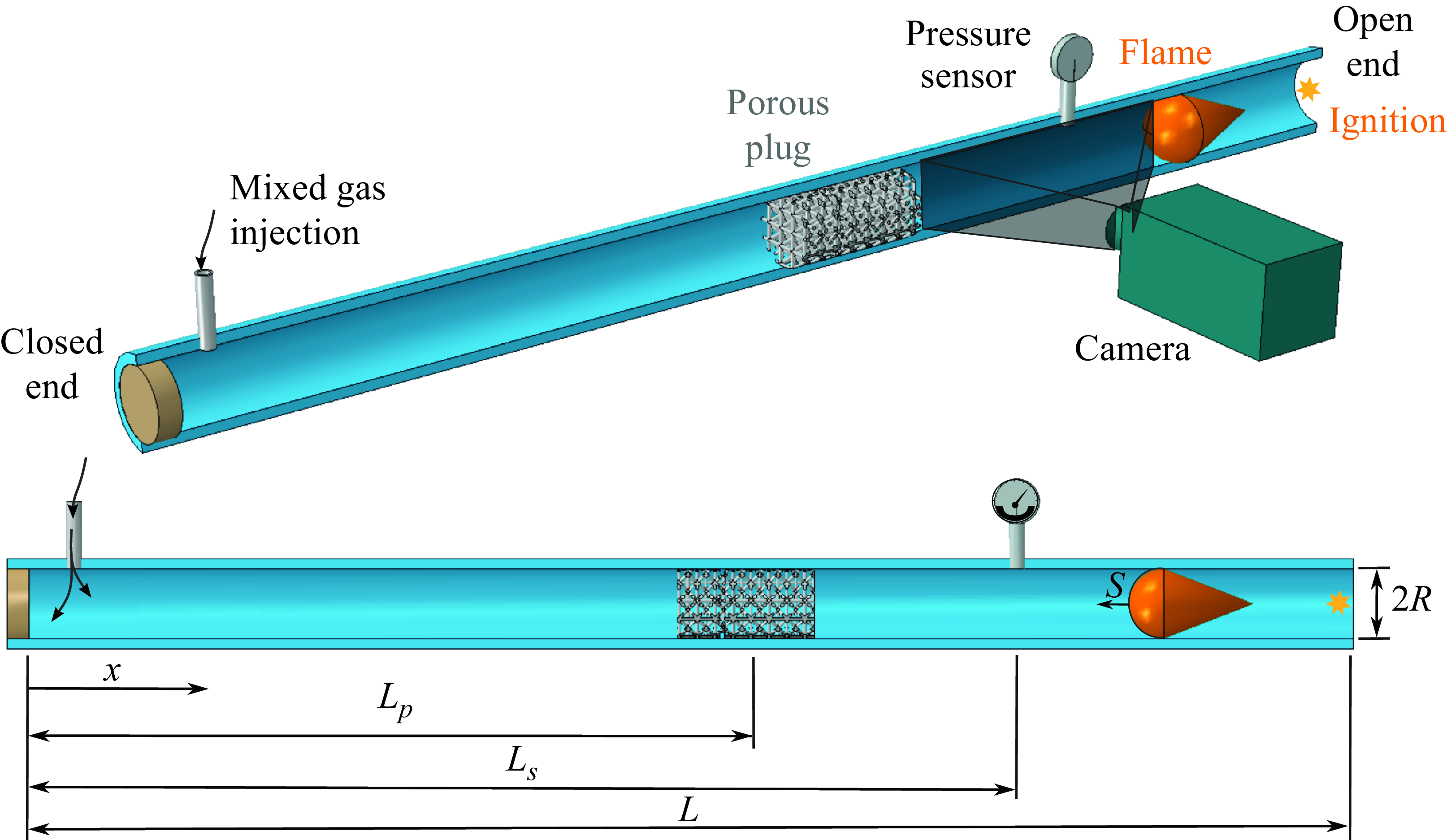
2. Experimental set-up and procedure
The objective of this study is to investigate the ability of a porous structure to mitigate thermoacoustic waves, discerning between acoustic mode alteration and viscous dissipation effects. A schematic of the experimental set-up and the combustion chamber is shown in figure 1. It consists of a polymethyl methacrylate (PMMA) slender tube with an inner diameter $D = 1.55\,\textrm{cm}$
and length
$D = 1.55\,\textrm{cm}$
and length $L = 160\,\textrm{cm}$
. At first, the tube is filled with a premixed methane and air mixture at a stoichiometric equivalence ratio prepared with two Bronkhorst EL-Flow mass flow controllers. After allowing for the gases to reach thermal equilibrium with the room and a state free from any inertial effects (60 s at
$L = 160\,\textrm{cm}$
. At first, the tube is filled with a premixed methane and air mixture at a stoichiometric equivalence ratio prepared with two Bronkhorst EL-Flow mass flow controllers. After allowing for the gases to reach thermal equilibrium with the room and a state free from any inertial effects (60 s at $25\,^\circ$
C), the ignition is produced at the open end with a low-energy piezoelectric spark plug, resulting in the propagation of a premixed flame towards the closed end of the tube. As the flame advances, the oscillations appear and spontaneously change in intensity and frequency along the combustion tube.
$25\,^\circ$
C), the ignition is produced at the open end with a low-energy piezoelectric spark plug, resulting in the propagation of a premixed flame towards the closed end of the tube. As the flame advances, the oscillations appear and spontaneously change in intensity and frequency along the combustion tube.
Diagram of the experimental set-up showing the ignition point, the porous plug, the high-speed camera and the pressure sensor. The flame propagates from the open end towards the closed end of the tube.
2.1. Pressure and flame-velocity measurements
The flame propagation is recorded using a Phantom VEO 710L high-speed camera with a resolution of $1280\times 150$
pixels and a frame rate of 2000 frames per second. Owing to the slenderness of the combustion chamber, where
$1280\times 150$
pixels and a frame rate of 2000 frames per second. Owing to the slenderness of the combustion chamber, where $L\gg D$
, and the need for spatial resolution across the flame front, only partial longitudinal visualisation of the set-up is possible during each run of the experiment. The position of the camera was fixed for all the experiments, capturing a field of view of the tube between
$L\gg D$
, and the need for spatial resolution across the flame front, only partial longitudinal visualisation of the set-up is possible during each run of the experiment. The position of the camera was fixed for all the experiments, capturing a field of view of the tube between $30$
and
$30$
and $60$
cm from the open end. Moreover, pressure oscillations inside the tube, above and below ambient pressure values, are measured with a couple of integrated silicon pressure transducers MPX5050 that are placed at a fixed position
$60$
cm from the open end. Moreover, pressure oscillations inside the tube, above and below ambient pressure values, are measured with a couple of integrated silicon pressure transducers MPX5050 that are placed at a fixed position $L_s = 2L/3$
, i.e. at a distance of 106.6 cm from the closed end. The sensors’ response time is
$L_s = 2L/3$
, i.e. at a distance of 106.6 cm from the closed end. The sensors’ response time is $1$
ms and pressure was sampled at
$1$
ms and pressure was sampled at $10$
kHz.
$10$
kHz.
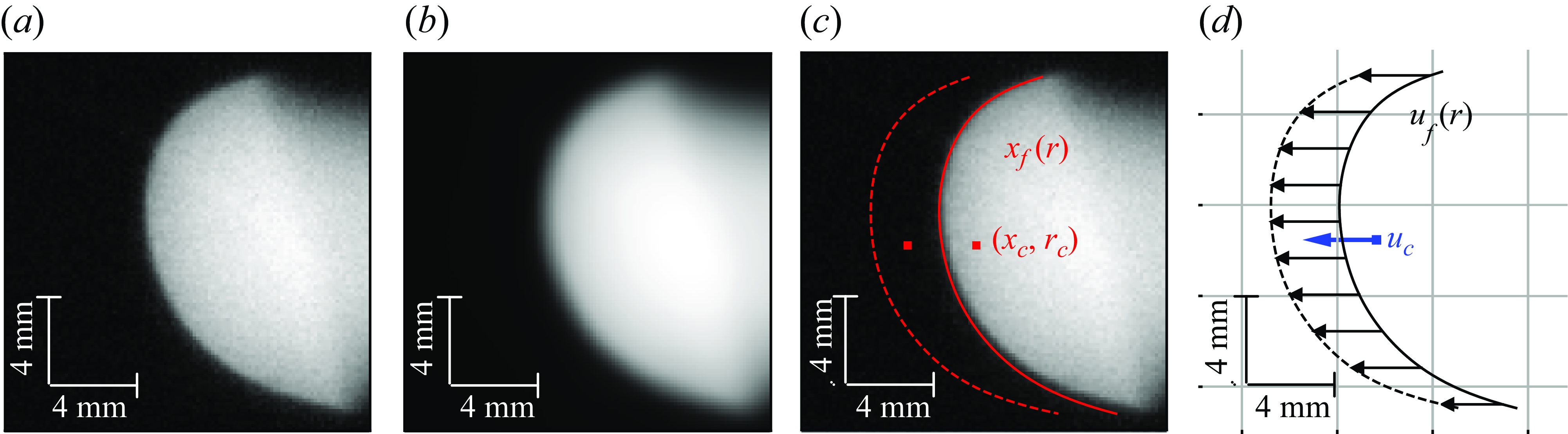
Each frame of the recorded video registers the instantaneous luminosity of the flame providing its position. The images are preprocessed using the denoising algorithm proposed by Rudin, Osher & Fatemi (Reference Rudin, Osher and Fatemi1992). This filter comprises an optimisation algorithm that solves a numerically derived Euler–Lagrange equation, using a priori information on noise statistics. The objective is to reduce the standard deviation of the image caused by the noise, while conserving flame-shape features. Subsequently, a detection algorithm is employed to extract the flame front from each image, as shown in figure 2. This is achieved by delineating a border between the light and dark pixels of the binarised image and retaining only the advancing-front side of the contour. The in-house algorithm is written in Python using the OpenCV library. The detected flame fronts are fitted by an eighth-degree polynomial which is enough to capture the flame’s deformation while removing the detection noise and improving subpixel resolution (Flores-Montoya et al. Reference Flores-Montoya, Muntean, Sánchez-Sanz and Martínez-Ruiz2022).
Raw image of the flame (a), filtered image (b), detection of the flame front as a function of the radial distance to the axis of the tube, $x_f(r)$
, and centroid’s position,
$x_f(r)$
, and centroid’s position, $(x_c,r_c)$
(c), flame and centroid velocity,
$(x_c,r_c)$
(c), flame and centroid velocity, $u_f(r)$
and
$u_f(r)$
and $u_c$
respectively (d).
$u_c$
respectively (d).
Once all the frames are filtered, the velocity of the flame along the axial direction can be computed by tracking its displacement between consecutive frames, separated by a time $t= 1/2000$
s. Therefore, the axial component of the velocity at each point
$t= 1/2000$
s. Therefore, the axial component of the velocity at each point $u_f$
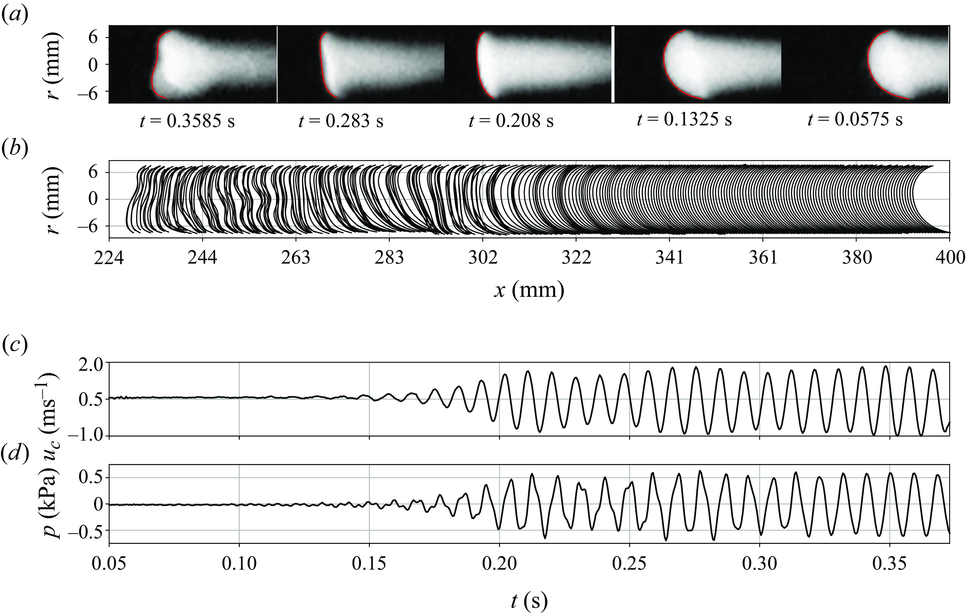
in the flame front is available, as well as the velocity of the centroid, which serves as a global flame variable. The flame oscillations and the modified flame shape that the thermoacoustic coupling produces in the unstable process are recorded as presented in figure 3. The (a) and (b) panels show the evolution of the flame propagation from right to left over time, together with the front detection in red superposed lines, and reproduced below for every two frames to track the propagation along
$u_f$
in the flame front is available, as well as the velocity of the centroid, which serves as a global flame variable. The flame oscillations and the modified flame shape that the thermoacoustic coupling produces in the unstable process are recorded as presented in figure 3. The (a) and (b) panels show the evolution of the flame propagation from right to left over time, together with the front detection in red superposed lines, and reproduced below for every two frames to track the propagation along $x$
. The (c) and (d) panels show the velocity oscillations as extracted from image processing and centroid detection
$x$
. The (c) and (d) panels show the velocity oscillations as extracted from image processing and centroid detection $u_c(t)$
, and pressure measurements of the experimental run
$u_c(t)$
, and pressure measurements of the experimental run $p(t)$
. The good accordance between both signals indicates that the flame-front dynamics behave initially as a passive interface subject to acoustic oscillations. However, these so-called primary instabilities can undergo a transition towards secondary regimes, where the flame is folded and actively modifies the coupling with the pressure oscillations that grow an order of magnitude larger. The characteristic behaviour and dynamics involved in this process have long been studied by different authors theoretically (Pelcé & Rochwerger Reference Pelcé and Rochwerger1992; Markstein & Squire Reference Markstein and Squire1955), in two-phase flows (Clanet, Searby & Clavin Reference Clanet, Searby and Clavin1999) and experimentally for various fuels (Martínez-Ruiz et al. Reference Martínez-Ruiz, Veiga-López and Sánchez-Sanz2019; Veiga-López et al. Reference Veiga-López, Martínez-Ruiz, Fernández-Tarrazo and Sánchez-Sanz2019).
$p(t)$
. The good accordance between both signals indicates that the flame-front dynamics behave initially as a passive interface subject to acoustic oscillations. However, these so-called primary instabilities can undergo a transition towards secondary regimes, where the flame is folded and actively modifies the coupling with the pressure oscillations that grow an order of magnitude larger. The characteristic behaviour and dynamics involved in this process have long been studied by different authors theoretically (Pelcé & Rochwerger Reference Pelcé and Rochwerger1992; Markstein & Squire Reference Markstein and Squire1955), in two-phase flows (Clanet, Searby & Clavin Reference Clanet, Searby and Clavin1999) and experimentally for various fuels (Martínez-Ruiz et al. Reference Martínez-Ruiz, Veiga-López and Sánchez-Sanz2019; Veiga-López et al. Reference Veiga-López, Martínez-Ruiz, Fernández-Tarrazo and Sánchez-Sanz2019).
Characteristic flame-front oscillation as observed from (a) high-speed images, (b) front tracking, (c) centroid propagation velocity $u_c$
and (d) pressure measurements
$u_c$
and (d) pressure measurements $p$
.
$p$
.
2.2. Porous plugs characterisation
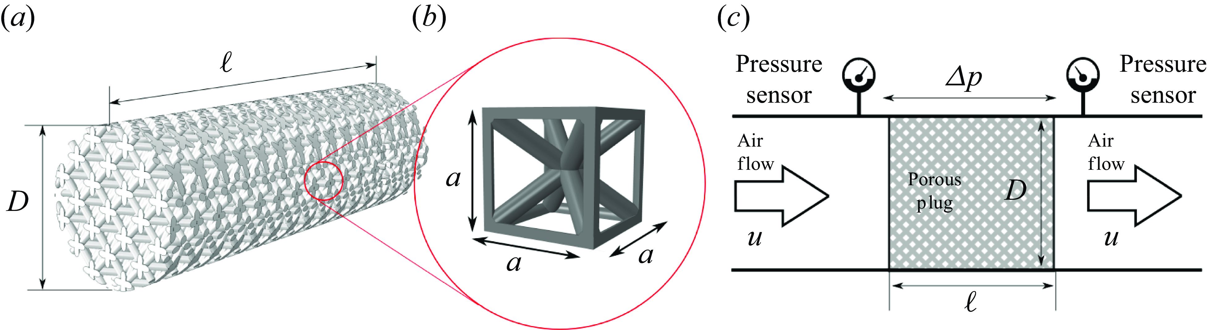
Prior to filling the tube with the gas mixture, a porous plug of diameter $D = 1.55\,\textrm{cm}$
, matching the inner diameter of the tube, is introduced and tightened in place by a rubber O-ring to prevent it from sliding. The position of the plug in the tube is fixed for each experimental run at a distance
$D = 1.55\,\textrm{cm}$
, matching the inner diameter of the tube, is introduced and tightened in place by a rubber O-ring to prevent it from sliding. The position of the plug in the tube is fixed for each experimental run at a distance $L_p$
from the closed end, measured at the border of the porous plug facing the open end. The lattice structure is displayed in figure 4(a), and is based on a combination of body-centred cubic and single cubic (BCC-SC) arrangements. Three unit-cell sizes
$L_p$
from the closed end, measured at the border of the porous plug facing the open end. The lattice structure is displayed in figure 4(a), and is based on a combination of body-centred cubic and single cubic (BCC-SC) arrangements. Three unit-cell sizes $a$
were considered, with values of
$a$
were considered, with values of $a=$
4.0, 3.0 and 2.0 mm. These elements are fabricated using low-force stereolithography and made of FormLabs© Clear Resin, which emulates the strength and rigidity of polyethylene. The diameter of the structure bars is 0.20 mm in all cases, while the printing layer resolution is 25 microns in height. Different unit-cell layouts, sizes
$a=$
4.0, 3.0 and 2.0 mm. These elements are fabricated using low-force stereolithography and made of FormLabs© Clear Resin, which emulates the strength and rigidity of polyethylene. The diameter of the structure bars is 0.20 mm in all cases, while the printing layer resolution is 25 microns in height. Different unit-cell layouts, sizes $a$
and plug lengths
$a$
and plug lengths $\ell$
, were characterised and tested in a predesign study. In fact, each unit-cell size
$\ell$
, were characterised and tested in a predesign study. In fact, each unit-cell size $a\in (2,3,4)$
mm was tested for different lengths of the porous plug
$a\in (2,3,4)$
mm was tested for different lengths of the porous plug $\ell \in (20,30,45)$
mm.
$\ell \in (20,30,45)$
mm.
The porous structures of this work were manufactured specifically to alter the thermoacoustic behaviour of the premixed-flame system at hand by means of viscous dissipation. In order to quantify this effect, some prior testing was required to characterise the permeability $K$
of the structures which is defined in accordance with Darcy’s law as
$K$
of the structures which is defined in accordance with Darcy’s law as
 \begin{equation} u = -\frac {K}{\mu } \frac {\Delta p}{\ell }, \end{equation}
where $\mu$
is the dynamic viscosity,
$\mu$
is the dynamic viscosity, $\Delta p$
is the pressure drop across the plug, and
$\Delta p$
is the pressure drop across the plug, and $u$
is the flow velocity. It should be noted that a constant pressure loss is considered, with linear velocity variation in the axial direction. Furthermore, figure 4(c) shows a schematic of the experimental set-up carried out to determine the permeability of different porous plug designs. The utilisation of linearised Darcy’s law as a model for the acoustic response is substantiated under the premise of low permeability and negligible inertial effects, conditions under which the flow remains within the linear regime. Despite the fact that this approximation may be subject to loss of accuracy at high frequencies, it remains valid within the operating range that has been considered in this work.
$u$
is the flow velocity. It should be noted that a constant pressure loss is considered, with linear velocity variation in the axial direction. Furthermore, figure 4(c) shows a schematic of the experimental set-up carried out to determine the permeability of different porous plug designs. The utilisation of linearised Darcy’s law as a model for the acoustic response is substantiated under the premise of low permeability and negligible inertial effects, conditions under which the flow remains within the linear regime. Despite the fact that this approximation may be subject to loss of accuracy at high frequencies, it remains valid within the operating range that has been considered in this work.
Illustration of the 3-D-printed porous plug (a), the lattice structure of a BCC-SC unit cell (b) and the experimental characterisation arrangement (c).
The characterisation experiments are performed by forcing a controlled mass flow rate of air through the porous plug, once fixed inside the PMMA tube. Pressure measurements were taken inside the tube at both ends of the plugs to measure the pressure drop for varying air velocity, $u \in (0.0,0.7)\,\textrm{m s}^-{^1}$
, which is in the range of the amplitude of the velocity oscillations observed in the thermoacoustic instabilities from the experiments.
$u \in (0.0,0.7)\,\textrm{m s}^-{^1}$
, which is in the range of the amplitude of the velocity oscillations observed in the thermoacoustic instabilities from the experiments.
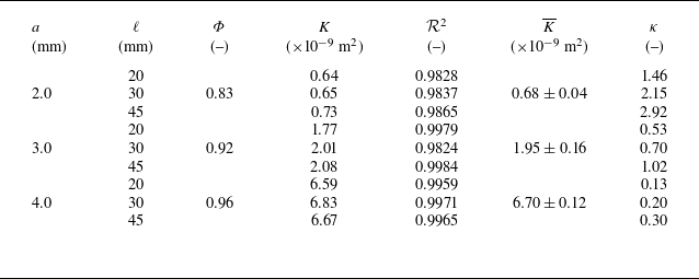
Table 1 presents the unit-cell size $a$
, the plug length
$a$
, the plug length $\ell$
, porosity
$\ell$
, porosity $\Phi$
as the ratio of empty to total volume, the experimentally obtained permeability
$\Phi$
as the ratio of empty to total volume, the experimentally obtained permeability $K$
and the coefficient of determination
$K$
and the coefficient of determination $\mathcal{R}^2$
, together with the mean and standard deviation value
$\mathcal{R}^2$
, together with the mean and standard deviation value $\overline {K}$
for each of the porous types considered in the study. In addition, we shall use a dimensionless parameter
$\overline {K}$
for each of the porous types considered in the study. In addition, we shall use a dimensionless parameter $\kappa ={\mu \ell }/(\rho _u c_u K)$
, which will be utilised to characterise the porous plugs. Here,
$\kappa ={\mu \ell }/(\rho _u c_u K)$
, which will be utilised to characterise the porous plugs. Here, $\mu$
,
$\mu$
, $\rho _u$
and
$\rho _u$
and $c_u$
are dynamic viscosity, density and speed of sound in the unburnt gas, respectively. The parameter
$c_u$
are dynamic viscosity, density and speed of sound in the unburnt gas, respectively. The parameter $\kappa$
represents the resistance to the flow and the porous plugs with the larger
$\kappa$
represents the resistance to the flow and the porous plugs with the larger $\kappa$
are those that produce a larger pressure drop. Finally, the linear fit of the experimental permeability returned an
$\kappa$
are those that produce a larger pressure drop. Finally, the linear fit of the experimental permeability returned an $\mathcal{R}^2$
value higher than 0.97.
$\mathcal{R}^2$
value higher than 0.97.
Unit-cell size $a$
, length
$a$
, length $\ell$
, porosity
$\ell$
, porosity $\Phi$
, permeability
$\Phi$
, permeability $K$
, the
$K$
, the $\mathcal{R}^2$
fit quality and dimensionless parameter
$\mathcal{R}^2$
fit quality and dimensionless parameter $\kappa$
for each porous structure. The values
$\kappa$
for each porous structure. The values $\overline {K}$
represent the mean values of permeability with their associated standard deviations.
$\overline {K}$
represent the mean values of permeability with their associated standard deviations.
Furthermore, the relationship between the pressure drop, $\Delta p$
, and the flow velocity,
$\Delta p$
, and the flow velocity, $u$
, can be expressed as
$u$
, can be expressed as
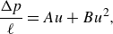 \begin{equation} \frac {\Delta p}{\ell } = {A} u + {B} u^2, \end{equation}
where $A$
and
$A$
and $B$
are constants determined by least-squares fitting. This model considers non-Darcy flow effects in single-phase flow by introducing relative permeability in the viscous term and the
$B$
are constants determined by least-squares fitting. This model considers non-Darcy flow effects in single-phase flow by introducing relative permeability in the viscous term and the $B$
factor in the inertial term (Fourar & Lenormand Reference Fourar and Lenormand2001; Bhattacharya, Calmidi & Mahajan Reference Bhattacharya, Calmidi and Mahajan2002; Nowamooz, Radilla & Fourar Reference Nowamooz, Radilla and Fourar2009). In fact, the constants enable the definition of the permeability
$B$
factor in the inertial term (Fourar & Lenormand Reference Fourar and Lenormand2001; Bhattacharya, Calmidi & Mahajan Reference Bhattacharya, Calmidi and Mahajan2002; Nowamooz, Radilla & Fourar Reference Nowamooz, Radilla and Fourar2009). In fact, the constants enable the definition of the permeability $K = \mu /{A}$
and the inertial coefficient
$K = \mu /{A}$
and the inertial coefficient $C_E = {B}\sqrt {K}/\rho _u$
(Ekade & Krishnan Reference Ekade and Krishnan2019).
$C_E = {B}\sqrt {K}/\rho _u$
(Ekade & Krishnan Reference Ekade and Krishnan2019).
Table 2 presents the permeability and inertia coefficient values determined based on the quadratic non-Darcy relationship for each of the porous plugs. The table also includes the corresponding mean values and standard deviations. The $\mathcal{R}^2$
parameter of the fit has been excluded from the presented data set, as it consistently exhibited a constant value of 0.99 in all cases.
$\mathcal{R}^2$
parameter of the fit has been excluded from the presented data set, as it consistently exhibited a constant value of 0.99 in all cases.
Geometric parameters of the unit cell ( $a$
) and characteristic length (
$a$
) and characteristic length ( $\ell$
), along with the permeability (
$\ell$
), along with the permeability ( $K$
) and the coefficient of inertia (C
$K$
) and the coefficient of inertia (C $_E$
) for each porous structure, as obtained from the non-Darcy flow relationship. The values
$_E$
) for each porous structure, as obtained from the non-Darcy flow relationship. The values $\overline {K}$
and
$\overline {K}$
and $\overline {{C}}_E$
represent the mean values of permeability and coefficient of inertia, respectively, with their associated standard deviations.
$\overline {{C}}_E$
represent the mean values of permeability and coefficient of inertia, respectively, with their associated standard deviations.

The results obtained from the characterisation tests for various porous structures are shown in figure 5. The symbols show the experimental measurements for $\ell= 20\,\textrm{mm}$
(triangles), 30 mm (squares) and 45 mm (circles), confirming that the permeability is governed only by the cell size
$\ell= 20\,\textrm{mm}$
(triangles), 30 mm (squares) and 45 mm (circles), confirming that the permeability is governed only by the cell size $a$
, regardless of the length
$a$
, regardless of the length $\ell$
. In addition, the graphs include the linear (dashed line) and quadratic (continuous line) fits for each series of experiments, which is the mean value obtained from three different lengths of each unit-cell size.
$\ell$
. In addition, the graphs include the linear (dashed line) and quadratic (continuous line) fits for each series of experiments, which is the mean value obtained from three different lengths of each unit-cell size.
Flow velocity as a function of pressure drop as tested experimentally (symbols) for unit-cell sizes of $a=4\,\textrm{mm}$
(green),
$a=4\,\textrm{mm}$
(green), $a=3\,\textrm{mm}$
(red) and
$a=3\,\textrm{mm}$
(red) and $a=2\,\textrm{mm}$
(blue), with their respective least-squares linear (dashed line) and quadratic (continuous line) fits.
$a=2\,\textrm{mm}$
(blue), with their respective least-squares linear (dashed line) and quadratic (continuous line) fits.
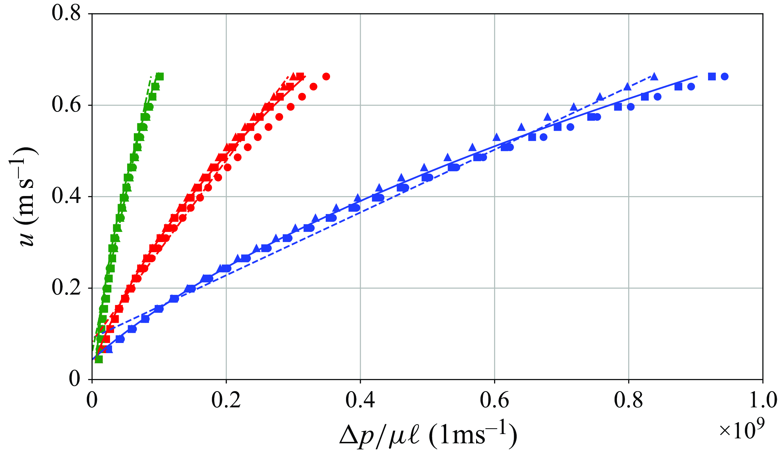
The linear and parabolic fittings return different values for the permeability $K$
. Among these options, the linear fitting is considered sufficient to describe the porous plug in this application since the acoustic velocity is much smaller than one for most of an acoustic cycle during primary instabilities. As a final remark, this characterisation using a steady flow is deemed acceptable to describe the porous plug’s properties under an oscillating flow. This is because the response time of a viscous flow in the pores which are approximately
$K$
. Among these options, the linear fitting is considered sufficient to describe the porous plug in this application since the acoustic velocity is much smaller than one for most of an acoustic cycle during primary instabilities. As a final remark, this characterisation using a steady flow is deemed acceptable to describe the porous plug’s properties under an oscillating flow. This is because the response time of a viscous flow in the pores which are approximately $\delta _p=0.2\,\textrm{mm}$
wide is of the order of
$\delta _p=0.2\,\textrm{mm}$
wide is of the order of $t_v\sim \rho _u\delta _p^2/\mu \approx 1 \times 10^{-3}$
s smaller than the typical acoustic period from the experiments
$t_v\sim \rho _u\delta _p^2/\mu \approx 1 \times 10^{-3}$
s smaller than the typical acoustic period from the experiments $t_a\approx 1 \times 10^{-2}$
s.
$t_a\approx 1 \times 10^{-2}$
s.
3. Theoretical model: non-isothermal acoustics with porous plug
This section presents a one-dimensional acoustic perturbation analysis developed from first principles to predict the effect on thermoacoustic instability eigenmodes of a porous structure and a premixed flame in a slender tube.
3.1. Governing equations
Firstly, the flow is considered to be one-dimensional due to the large aspect ratio of the tube, $L\gg D$
. The characteristic length scale of the acoustic problem is the tube length
$L\gg D$
. The characteristic length scale of the acoustic problem is the tube length $L$
, along which the acoustic waves travel at the local speed of sound
$L$
, along which the acoustic waves travel at the local speed of sound $c=\sqrt {\gamma p/ \rho }$
, where
$c=\sqrt {\gamma p/ \rho }$
, where $\gamma$
is the ratio of specific heats of the gas. Consequently, the length scales of the plugs
$\gamma$
is the ratio of specific heats of the gas. Consequently, the length scales of the plugs $\ell$
, and flame thickness
$\ell$
, and flame thickness $\delta _T$
are much smaller than the tube length,
$\delta _T$
are much smaller than the tube length, $L\gg \ell \gg \delta _T$
. Therefore, both the porous plugs and the flame are treated as surfaces of discontinuity in the acoustics problem. Acoustics within the porous plug are neglected based on the length difference
$L\gg \ell \gg \delta _T$
. Therefore, both the porous plugs and the flame are treated as surfaces of discontinuity in the acoustics problem. Acoustics within the porous plug are neglected based on the length difference $\ell /L \ll 1$
.
$\ell /L \ll 1$
.
The subscript ‘ $u$
’ refers to the unburnt gas conditions where
$u$
’ refers to the unburnt gas conditions where $\rho _u$
and
$\rho _u$
and $T_u$
define the density and temperature of the unburnt gas, respectively. The characteristic acoustic time
$T_u$
define the density and temperature of the unburnt gas, respectively. The characteristic acoustic time $t_a=L/c_u$
is referred to the cold-gas speed of sound
$t_a=L/c_u$
is referred to the cold-gas speed of sound $c_u$
, and is much shorter than the flame residence time
$c_u$
, and is much shorter than the flame residence time $t_r = L/S$
, where
$t_r = L/S$
, where $S$
is the flame propagation speed. In terms of the acoustic problem, the flame-induced flow field can be considered as quasi-steady. The dimensionless coordinate and time are given by
$S$
is the flame propagation speed. In terms of the acoustic problem, the flame-induced flow field can be considered as quasi-steady. The dimensionless coordinate and time are given by $\xi ={x/L}$
and
$\xi ={x/L}$
and $\tau ={t}/{t_a}$
, respectively. Furthermore, the dimensionless flow variables such as velocity
$\tau ={t}/{t_a}$
, respectively. Furthermore, the dimensionless flow variables such as velocity $\hat {u}$
, density
$\hat {u}$
, density $\hat {\rho }$
, temperature
$\hat {\rho }$
, temperature $\hat {T}$
and pressure
$\hat {T}$
and pressure $\hat {p}$
arise from rescaling with the characteristic flame speed
$\hat {p}$
arise from rescaling with the characteristic flame speed $S$
, unburnt density
$S$
, unburnt density $\rho _u$
, temperature
$\rho _u$
, temperature $T_u$
and acoustic pressure
$T_u$
and acoustic pressure $\rho _u c_u S$
. Dimensionless conservation equations for mass, momentum and energy are written, with viscous and dissipative terms neglected, as
$\rho _u c_u S$
. Dimensionless conservation equations for mass, momentum and energy are written, with viscous and dissipative terms neglected, as
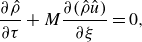 \begin{align} \frac {\partial \hat {\rho }}{\partial \tau } + M \frac {\partial ( \hat {\rho } \hat {u})}{\partial \xi }= 0, \end{align}
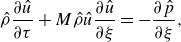 \begin{align} \hat {\rho }\frac {\partial \hat {u}}{\partial \tau } + M \hat {\rho } \hat {u} \frac {\partial \hat {u}}{\partial \xi } = -\frac {\partial \hat {p}}{\partial \xi }, \end{align}
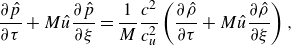 \begin{align} \frac {\partial \hat {p}}{\partial \tau } + M \hat {u} \frac {\partial \hat {p} }{\partial \xi } = \frac {1}{M}\frac {c^2}{c_u^2}\left ( \frac {\partial \hat {\rho }}{\partial \tau } + M \hat {u}\frac {\partial \hat {\rho }}{\partial \xi }\right ), \end{align}
where the flame propagation Mach number $M = S/c_u$
is low, and use is made of the ideal gas equation of state.
$M = S/c_u$
is low, and use is made of the ideal gas equation of state.
These flow-field variables are split into a quasi-steady base flow and acoustic perturbations, as $\hat {\psi }(x,t) = \psi _0(x) + \psi '(x,t)$
. It should be noted that from linearised isentropic acoustics, density perturbations
$\hat {\psi }(x,t) = \psi _0(x) + \psi '(x,t)$
. It should be noted that from linearised isentropic acoustics, density perturbations $\rho ' \simeq p' M\ll p'$
should not be retained. First-order perturbations in the linearised system enable writing the wave equations for velocity and pressure as
$\rho ' \simeq p' M\ll p'$
should not be retained. First-order perturbations in the linearised system enable writing the wave equations for velocity and pressure as
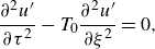 \begin{align}\frac {\partial ^2 u'}{\partial \tau ^2} - T_0 \frac {\partial ^2 u'}{\partial \xi ^2} = 0,\end{align}
 \begin{align} \frac {\partial ^2 p'}{\partial \tau ^2} - \frac {\partial }{\partial \xi } \left ( T_0 \frac {\partial p'}{\partial \xi }\right ) = 0, \end{align}
where $T_0 = c^2/c_u^2$
arises from consideration of non-isothermal acoustics and local variation of the speed of sound. Note that the characteristic time variation of the temperature profile along the tube is, in first order, directly linked to the flame residence time. The latter is much longer than the acoustic time of pressure wave propagation,
$T_0 = c^2/c_u^2$
arises from consideration of non-isothermal acoustics and local variation of the speed of sound. Note that the characteristic time variation of the temperature profile along the tube is, in first order, directly linked to the flame residence time. The latter is much longer than the acoustic time of pressure wave propagation, $t_r/t_a \sim O(M^{-1})\gg 1$
. Therefore, the one-dimensional temperature distribution can be considered as a quasi-steady function of the flame position
$t_r/t_a \sim O(M^{-1})\gg 1$
. Therefore, the one-dimensional temperature distribution can be considered as a quasi-steady function of the flame position $\xi _f = L_f/L$
. Finally, the domain is split in two regions at either side of the porous plug location,
$\xi _f = L_f/L$
. Finally, the domain is split in two regions at either side of the porous plug location, $\xi _p= L_p/L$
, which will be referred to as closed side and open side depending on their end of the tube.
$\xi _p= L_p/L$
, which will be referred to as closed side and open side depending on their end of the tube.
In order to close the set of wave equations, the following boundary conditions are applied. At the porous discontinuity, the flame is always arrested and the density remains equal to the initial reactant mixture, hence a constant mass flow must be imposed $u'({\xi _p^-}) = u'({\xi _p^+})$
, where superscripts
$u'({\xi _p^-}) = u'({\xi _p^+})$
, where superscripts $+$
and
$+$
and $-$
indicate a position slightly after or before
$-$
indicate a position slightly after or before $\xi _p$
. Moreover, the pressure drop therein is set by Darcy’s law in (2.1), specifically
$\xi _p$
. Moreover, the pressure drop therein is set by Darcy’s law in (2.1), specifically $[p'(\xi _p^+) - p'(\xi _p^-)] = - \kappa u'(\xi _p)$
, where the dimensionless parameter of the porous structure
$[p'(\xi _p^+) - p'(\xi _p^-)] = - \kappa u'(\xi _p)$
, where the dimensionless parameter of the porous structure $\kappa ={\mu \ell }/({\rho _u c_u K})$
is recalled here for convenience. Then, additional boundary conditions are prescribed at the closed end,
$\kappa ={\mu \ell }/({\rho _u c_u K})$
is recalled here for convenience. Then, additional boundary conditions are prescribed at the closed end, $u'(\xi =0) = 0$
, and open end, that in first approximation remains at atmospheric pressure,
$u'(\xi =0) = 0$
, and open end, that in first approximation remains at atmospheric pressure, $p'(\xi =1) = 0$
.
$p'(\xi =1) = 0$
.
The acoustics solution of (3.4)–(3.5) at either side of $\xi _p$
is expected to be of the form
$\xi _p$
is expected to be of the form $p'= e^{i\Omega \tau } [A \phi (\xi ) + B ]$
, with the normalised eigenvalue
$p'= e^{i\Omega \tau } [A \phi (\xi ) + B ]$
, with the normalised eigenvalue $\Omega =\omega t_a$
, referred to the angular frequency of an oscilation
$\Omega =\omega t_a$
, referred to the angular frequency of an oscilation $\omega$
and the acoustic time
$\omega$
and the acoustic time $t_a$
. The real part
$t_a$
. The real part $\Omega _r$
of the complex eigenvalue indicates the frequency of each mode, whereas the imaginary part
$\Omega _r$
of the complex eigenvalue indicates the frequency of each mode, whereas the imaginary part $\Omega _i$
denotes the damping or amplification of the modes. When the imaginary part is positive the modes are damped.
$\Omega _i$
denotes the damping or amplification of the modes. When the imaginary part is positive the modes are damped.
Moreover, $\phi (\xi )$
represents the eigenfunctions which, for isothermal porousless acoustic problems, recover the classic
$\phi (\xi )$
represents the eigenfunctions which, for isothermal porousless acoustic problems, recover the classic $\sin$
–
$\sin$
– $\cos$
solutions. Since the time dependence of the variable profiles is prescribed, Euler momentum (3.2) can be used as
$\cos$
solutions. Since the time dependence of the variable profiles is prescribed, Euler momentum (3.2) can be used as $i\Omega u' =- T_0 {\partial p'}/{\partial \xi }$
to replace the variable
$i\Omega u' =- T_0 {\partial p'}/{\partial \xi }$
to replace the variable $u'$
by
$u'$
by $p'$
. The end-tube and additional porous boundary conditions over the pressure perturbation variable are
$p'$
. The end-tube and additional porous boundary conditions over the pressure perturbation variable are
 \begin{align} \left .\frac {\partial p'}{\partial \xi }\right |_{\xi _p^-} = \left .\frac {\partial p'}{\partial \xi }\right |_{\xi _p^+}; \quad p'(\xi _p^+) - p'(\xi _p^-) =\left . \frac {\kappa }{i\Omega }\frac {\partial p'}{\partial \xi }\right |_{\xi _p}; \quad \left .\frac {\partial p'}{\partial \xi }\right |_{0} = 0; \quad p'(1) = 0.\nonumber\\[-5pt] \end{align}
Accurate modelling calls for incorporating the slowly varying temperature field owing to the propagation of the flame. The classical strategy followed by Clavin, Pelcé & He (Reference Clavin, Pelcé and He1990) incorporates two distinct regions separated by the flame position at unburnt $T_0=1$
and burnt
$T_0=1$
and burnt $T_0 = \epsilon$
temperatures, where
$T_0 = \epsilon$
temperatures, where $\epsilon$
is defined as the temperature ratio through the flame. However, experimental evidence in slender tubes shows a non-negligible mismatch of the self-excited acoustic frequencies owing to the non-adiabatic nature of the system and temperature decay after the flame as proposed by Flores-Montoya et al. (Flores-Montoya et al. Reference Flores-Montoya, Muntean, Sánchez-Sanz and Martínez-Ruiz2022). Therein, good frequency agreement with experimental results is provided via the estimation of the length affected by conductive heat losses through the tube’s wall
$\epsilon$
is defined as the temperature ratio through the flame. However, experimental evidence in slender tubes shows a non-negligible mismatch of the self-excited acoustic frequencies owing to the non-adiabatic nature of the system and temperature decay after the flame as proposed by Flores-Montoya et al. (Flores-Montoya et al. Reference Flores-Montoya, Muntean, Sánchez-Sanz and Martínez-Ruiz2022). Therein, good frequency agreement with experimental results is provided via the estimation of the length affected by conductive heat losses through the tube’s wall $l_c ={4 u_b D^2}/({Nu} D_T)$
. This length is extracted from the solution of a section-averaged heat transport problem in a tube with the burnt-gas speed
$l_c ={4 u_b D^2}/({Nu} D_T)$
. This length is extracted from the solution of a section-averaged heat transport problem in a tube with the burnt-gas speed $u_b$
, thermal diffusivity
$u_b$
, thermal diffusivity $D_T$
and characteristic Nusselt number value in pipe flows,
$D_T$
and characteristic Nusselt number value in pipe flows, ${Nu}=3.66$
. Therefore, the region ahead of the flame (
${Nu}=3.66$
. Therefore, the region ahead of the flame ( $\xi \lt \xi _f$
) remains at initial temperature
$\xi \lt \xi _f$
) remains at initial temperature $T_0=1$
, while the burnt region (
$T_0=1$
, while the burnt region ( $\xi \gt \xi _f$
) can be described as
$\xi \gt \xi _f$
) can be described as
 \begin{equation} T_0(\xi ) = 1 + (\epsilon -1)\exp [-\sigma (\xi - \xi _f)], \end{equation}
with use made of the dimensionless parameter $\sigma ={L}/{l_c}={({Nu}/{Pe}) (L/D)^2}$
, constant for a given flame temperature (or air–fuel mixture) and tube aspect ratio
$\sigma ={L}/{l_c}={({Nu}/{Pe}) (L/D)^2}$
, constant for a given flame temperature (or air–fuel mixture) and tube aspect ratio $L/D$
, with
$L/D$
, with ${Pe}={L u_b}/{D_T}$
the Péclet number. If an average flame velocity of 0.50 m s–1 is considered, and for the testing conditions analysed in this work, it can be obtained that
${Pe}={L u_b}/{D_T}$
the Péclet number. If an average flame velocity of 0.50 m s–1 is considered, and for the testing conditions analysed in this work, it can be obtained that $\sigma =11$
.
$\sigma =11$
.
In our generic non-isothermal acoustics, a new pair of boundary conditions are required at the flame location $\xi _f$
, assuming small pressure variations through the flame in the low-Mach propagation regime and continuity in velocity perturbations:
$\xi _f$
, assuming small pressure variations through the flame in the low-Mach propagation regime and continuity in velocity perturbations:
 \begin{equation} p'\big(\xi _f^-\big) = p'\big(\xi _f^+\big); \qquad \left .\frac {\partial p'}{\partial \xi }\right |_{\xi _f^-} = \left .\epsilon \frac {\partial p'}{\partial \xi }\right |_{\xi _f^+}. \end{equation}
This set of boundary conditions along with $T_0(\xi )$
successfully predicts the system’s eigenmodes in the cited works. Thermoacoustic instabilities originate from the flame’s unsteady heat release which depends on the flame-front dynamics during the propagation, and no information on it is included in the model. Most importantly, the frequency of oscillation is prescribed by the set-up, tube length, boundary conditions and gas temperature distribution, which can be defined with a passive flame front. The self-amplification arises only when the flame is in certain areas such that the propagation time of a pressure wave from the flame to the end of the tube and back matches the flame response delay (Crocco Reference Crocco1951; Poinsot Reference Poinsot2005; Flores-Montoya et al. Reference Flores-Montoya, Muntean, Pozo-Estivariz and Martínez-Ruiz2023). These regions of instability inside the tube are expected to be slightly shifted due to the presence of the porous plugs, but these corrections go beyond the scope of this work.
$T_0(\xi )$
successfully predicts the system’s eigenmodes in the cited works. Thermoacoustic instabilities originate from the flame’s unsteady heat release which depends on the flame-front dynamics during the propagation, and no information on it is included in the model. Most importantly, the frequency of oscillation is prescribed by the set-up, tube length, boundary conditions and gas temperature distribution, which can be defined with a passive flame front. The self-amplification arises only when the flame is in certain areas such that the propagation time of a pressure wave from the flame to the end of the tube and back matches the flame response delay (Crocco Reference Crocco1951; Poinsot Reference Poinsot2005; Flores-Montoya et al. Reference Flores-Montoya, Muntean, Pozo-Estivariz and Martínez-Ruiz2023). These regions of instability inside the tube are expected to be slightly shifted due to the presence of the porous plugs, but these corrections go beyond the scope of this work.
Given these two surfaces of discontinuity at $\xi _p$
and
$\xi _p$
and $\xi _f$
, the domain is subdivided into three regions, namely the closed end to porous plug (
$\xi _f$
, the domain is subdivided into three regions, namely the closed end to porous plug ( $\xi \lt \xi _p$
), porous plug to flame (
$\xi \lt \xi _p$
), porous plug to flame ( $\xi _p\lt \xi \lt \xi _f$
) and flame to open end (
$\xi _p\lt \xi \lt \xi _f$
) and flame to open end ( $\xi _f\lt \xi$
), where (3.5) must be solved for six unknown constants,
$\xi _f\lt \xi$
), where (3.5) must be solved for six unknown constants, $A_i$
and
$A_i$
and $B_i$
, with the six boundary conditions written in the pressure perturbation variable, as defined in (3.6) and (3.8).
$B_i$
, with the six boundary conditions written in the pressure perturbation variable, as defined in (3.6) and (3.8).
Then, the eigenvalue problem must be computed numerically as a function of the non-homogeneous temperature, density and speed of sound. The spatial function $\phi$
and its derivatives are discretised over equispaced
$\phi$
and its derivatives are discretised over equispaced $\xi$
coordinates with a second-order finite difference scheme. The numerical eigenvalues,
$\xi$
coordinates with a second-order finite difference scheme. The numerical eigenvalues, $\lambda _n=-\Omega _n^2$
, and eigenfunctions
$\lambda _n=-\Omega _n^2$
, and eigenfunctions $\phi _n$
of (3.5) carry the additional complexity of
$\phi _n$
of (3.5) carry the additional complexity of $\Omega$
appearing as a parameter in the algebraic system through the boundary conditions in (3.6), which calls for an iterative solver.
$\Omega$
appearing as a parameter in the algebraic system through the boundary conditions in (3.6), which calls for an iterative solver.
Figure 6(a) shows the frequency variation of different modes, fundamental and first harmonic, with the position of the flame $\xi _f$
in the absence of porous media. In particular, the isothermal solution in the absence of the porous plug is plotted (solid line) in comparison with the adiabatic flame model of Clavin (Clavin et al. Reference Clavin, Pelcé and He1990) (dashed line) and the complete numerical solution with heat losses of Flores-Montoya (Flores-Montoya et al. Reference Flores-Montoya, Muntean, Sánchez-Sanz and Martínez-Ruiz2022) (dash-dotted line). In addition, figure 6(b–d) shows the new effect of permeability through the variation of
$\xi _f$
in the absence of porous media. In particular, the isothermal solution in the absence of the porous plug is plotted (solid line) in comparison with the adiabatic flame model of Clavin (Clavin et al. Reference Clavin, Pelcé and He1990) (dashed line) and the complete numerical solution with heat losses of Flores-Montoya (Flores-Montoya et al. Reference Flores-Montoya, Muntean, Sánchez-Sanz and Martínez-Ruiz2022) (dash-dotted line). In addition, figure 6(b–d) shows the new effect of permeability through the variation of $\kappa$
for three different locations of the porous plug,
$\kappa$
for three different locations of the porous plug, $\xi _p = 1/6$
,
$\xi _p = 1/6$
, $\xi _p = 1/3$
and
$\xi _p = 1/3$
and $\xi _p = 1/2$
, respectively. It can be noted that the eigenmode frequencies drift away from the porousless case for increasing
$\xi _p = 1/2$
, respectively. It can be noted that the eigenmode frequencies drift away from the porousless case for increasing $\kappa$
and
$\kappa$
and $\xi _p$
.
$\xi _p$
.
Real part of the eigenvalues $\Omega$
depending on the flame location
$\Omega$
depending on the flame location $\xi _f$
for
$\xi _f$
for ${(a)}$
adiabatic (
${(a)}$
adiabatic ( $\sigma =0$
) and non-adiabatic (
$\sigma =0$
) and non-adiabatic ( $\sigma \gt 0$
) wall solutions without porous plug,
$\sigma \gt 0$
) wall solutions without porous plug, ${(b)}$
for porous location
${(b)}$
for porous location $\xi _p=1/6$
and various
$\xi _p=1/6$
and various $\kappa$
,
$\kappa$
, ${(c)}$ $\xi _p=1/3$
,
$\xi _p=1/3$
, ${(d)}$ $\xi _p=1/2$
. In all cases the heat-loss parameter is
$\xi _p=1/2$
. In all cases the heat-loss parameter is $\sigma =11$
. Horizontal solid lines are the eigenvalues of the porousless, flameless case. The colour of the markers indicates the damping
$\sigma =11$
. Horizontal solid lines are the eigenvalues of the porousless, flameless case. The colour of the markers indicates the damping $\Omega _i$
.
$\Omega _i$
.

Moreover, $\Omega$
is as sensitive to the location of the porous plug
$\Omega$
is as sensitive to the location of the porous plug $\xi _p$
as it is to
$\xi _p$
as it is to $\kappa$
, but the effect of these two parameters on
$\kappa$
, but the effect of these two parameters on $\Omega$
shows a complex trend that is hard to infer from figure 6 alone. To address this effect, the analysis of a simplified case of acoustics in the absence of flame, with
$\Omega$
shows a complex trend that is hard to infer from figure 6 alone. To address this effect, the analysis of a simplified case of acoustics in the absence of flame, with $\epsilon =1$
,
$\epsilon =1$
, $T_0=1$
(isothermal) and without imposing jump conditions (3.8), reduces to the analytic expression
$T_0=1$
(isothermal) and without imposing jump conditions (3.8), reduces to the analytic expression
 \begin{equation} i\kappa \sin (\Omega (2\xi _p-1))-2\cos (\Omega ) + i\kappa \sin (\Omega )=0. \end{equation}
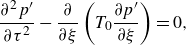
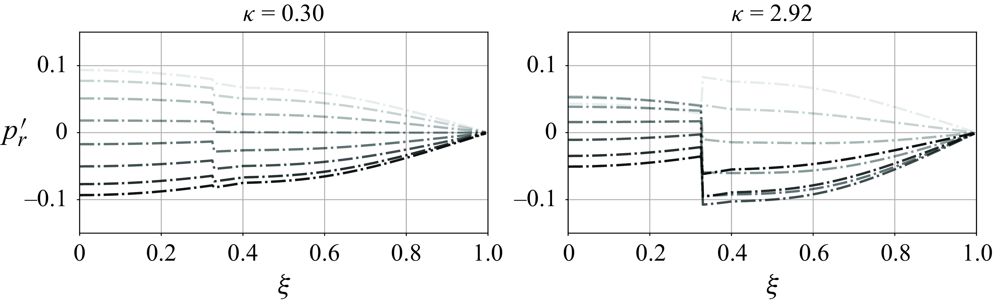
Here, the solution eigenfrequencies and damping of the system depend only on the permeability and location of the porous plug, represented together in figure 7. The limits of small $\kappa$
and
$\kappa$
and $\kappa \rightarrow \infty$
correspond respectively to a porousless case and the case with an impermeable wall at
$\kappa \rightarrow \infty$
correspond respectively to a porousless case and the case with an impermeable wall at $\xi _p$
. For
$\xi _p$
. For $\kappa =0.30$
, the
$\kappa =0.30$
, the $\Omega _r(\xi _p)$
curves remain on top of the porousless frequencies, while the damping
$\Omega _r(\xi _p)$
curves remain on top of the porousless frequencies, while the damping $\Omega _i$
takes its largest values when
$\Omega _i$
takes its largest values when $\xi _p$
sits near the pressure nodes, which are at
$\xi _p$
sits near the pressure nodes, which are at $\xi =1$
for the fundamental mode,
$\xi =1$
for the fundamental mode, $\xi =1/3$
and
$\xi =1/3$
and $\xi =1$
for the first harmonic and
$\xi =1$
for the first harmonic and $\xi =1/5$
,
$\xi =1/5$
, $\xi =3/5$
and
$\xi =3/5$
and $\xi =1$
for the second harmonic. It is not surprising that these are the most-dissipating placements as the velocity of the standing waves is maximal there, causing the greatest dissipation at the porous plug. For
$\xi =1$
for the second harmonic. It is not surprising that these are the most-dissipating placements as the velocity of the standing waves is maximal there, causing the greatest dissipation at the porous plug. For $\kappa = 2.92$
, the
$\kappa = 2.92$
, the $\Omega _r(\xi _p)$
curves change dramatically, approaching those of a solid plug. This is visible in the formation of a series of increasing branches of
$\Omega _r(\xi _p)$
curves change dramatically, approaching those of a solid plug. This is visible in the formation of a series of increasing branches of $\Omega _r$
that correspond to the modes on the open side of the tube becoming shorter, meanwhile a set of decreasing branches correspond to modes of the closed side of the tube whose frequency decreases as this side becomes larger.
$\Omega _r$
that correspond to the modes on the open side of the tube becoming shorter, meanwhile a set of decreasing branches correspond to modes of the closed side of the tube whose frequency decreases as this side becomes larger.
Real $\Omega _r$
and imaginary
$\Omega _r$
and imaginary $\Omega _i$
(colourbar) parts of the eigenmodes of a flameless tube (
$\Omega _i$
(colourbar) parts of the eigenmodes of a flameless tube ( $T_0=1$
) against the location of the porous plug location for
$T_0=1$
) against the location of the porous plug location for $\kappa = 0.3$
(a) and
$\kappa = 0.3$
(a) and $\kappa = 2.92$
(b). Horizontal solid lines are the eigenvalues of the porousless, flameless case.
$\kappa = 2.92$
(b). Horizontal solid lines are the eigenvalues of the porousless, flameless case.
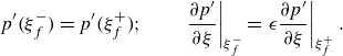
The eigenfunctions $\phi (\xi )=\phi _r(\xi )+i\phi _i(\xi )$
are complex-valued as well as the eigenvalues, so the real part of the solution for the pressure perturbations is
$\phi (\xi )=\phi _r(\xi )+i\phi _i(\xi )$
are complex-valued as well as the eigenvalues, so the real part of the solution for the pressure perturbations is $p'_r=e^{-\Omega _i\tau } [\phi _r(\xi )\cos (\Omega _r \tau )-\phi _i(\xi )\sin (\Omega _r\tau ) ]$
. In
$p'_r=e^{-\Omega _i\tau } [\phi _r(\xi )\cos (\Omega _r \tau )-\phi _i(\xi )\sin (\Omega _r\tau ) ]$
. In $p'_r$
, two standing waves
$p'_r$
, two standing waves $\phi _r$
and
$\phi _r$
and $\phi _i$
coexist and they oscillate with a
$\phi _i$
coexist and they oscillate with a $\pi /2$
phase lag one to the other. The shape of the fundamental and first-harmonic modes can be observed in figure 8, where
$\pi /2$
phase lag one to the other. The shape of the fundamental and first-harmonic modes can be observed in figure 8, where $\Omega _i$
is set to zero to represent the oscillating part of
$\Omega _i$
is set to zero to represent the oscillating part of $p'$
aside from the damping process. The symbols correspond to the location of the mode in the frequency panel of figure 7(b). It can be noted that both modes involve a greater number of nodes when placing the porous plug closer to the open end (figure 8
b,d). Therefore, a modification of both the frequencies and the characteristic acoustic pressure modes are expected when including this kind of dissipative media in the experimental set-up.
$p'$
aside from the damping process. The symbols correspond to the location of the mode in the frequency panel of figure 7(b). It can be noted that both modes involve a greater number of nodes when placing the porous plug closer to the open end (figure 8
b,d). Therefore, a modification of both the frequencies and the characteristic acoustic pressure modes are expected when including this kind of dissipative media in the experimental set-up.
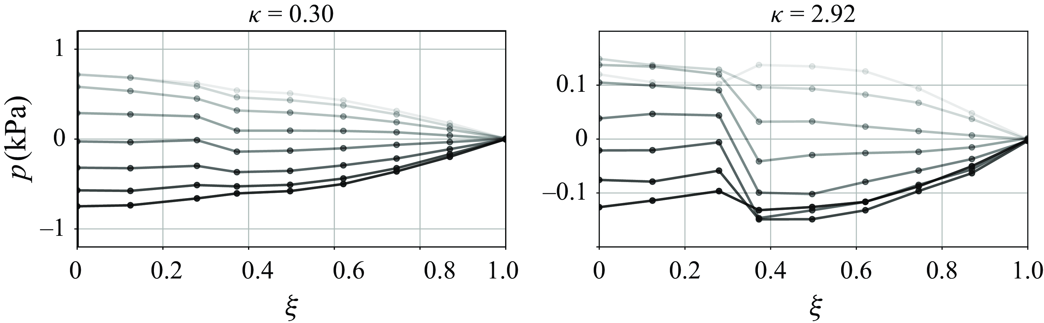
Theoretical acoustic perturbations $p'$
in the absence of a flame of the fundamental (a,b) and first-harmonic (c,d) modes for two locations of the porous plug
$p'$
in the absence of a flame of the fundamental (a,b) and first-harmonic (c,d) modes for two locations of the porous plug $\xi _p = 0.2$
(a,c) and
$\xi _p = 0.2$
(a,c) and $\xi _p = 0.85$
(b,d) with
$\xi _p = 0.85$
(b,d) with $\kappa =2.92$
. Instantaneous values are shown every one twentieth of the acoustic period from the lighter to the darker shades of grey.
$\kappa =2.92$
. Instantaneous values are shown every one twentieth of the acoustic period from the lighter to the darker shades of grey.
Porous plugs are often modelled through their impedance in Fourier space. The impedance is a complex number whose real part (the resistance) is related to the damping while its imaginary part (the reactance) is related to the lag of the pressure signal across the porous plug (Morse & Ingard Reference Morse and Ingard1986). Nevertheless, the present description in the time domain using Darcy’s law implicitly contains the equivalent damping $\Omega _i$
and lag effects of the impedance, as shown in figure 8.
$\Omega _i$
and lag effects of the impedance, as shown in figure 8.
4. Results
This section presents the experimental measurements and the agreement of the theoretical model, with the aim of providing further insight into the control of flame instabilities. The results regarding the efficiency of the porous plugs in mitigating thermoacoustic waves are evaluated based on the characteristics of the porous plug, acoustic measurements and high-speed camera recordings. Thereafter, the predictions of the proposed model and the physical analyses are discussed.
4.1. Pressure measurements
First, figure 9 shows the theoretical prediction of the fundamental mode of acoustic pressure for two porous plugs of different $\kappa$
placed at the same location
$\kappa$
placed at the same location $\xi _p=1/3$
and with the same flame position
$\xi _p=1/3$
and with the same flame position $\xi _f=0.4$
. Both cases show similar changes of slope at
$\xi _f=0.4$
. Both cases show similar changes of slope at $\xi _f$
owing to the same flame discontinuity but are noticeably different around the porous position. Curves are taken every
$\xi _f$
owing to the same flame discontinuity but are noticeably different around the porous position. Curves are taken every $\Delta \tau =0.2$
from the lightest shade of grey with
$\Delta \tau =0.2$
from the lightest shade of grey with $\Omega _i=0$
to avoid including damping dynamics. The pressure wave at the closed side of the porous plug lags behind the open side’s, providing a greater difference for higher
$\Omega _i=0$
to avoid including damping dynamics. The pressure wave at the closed side of the porous plug lags behind the open side’s, providing a greater difference for higher $\kappa$
values. Moreover, figure 10 presents the experimental validation of the acoustic mode when recording pressure variations at nine positions of the tube simultaneously. Curves are plotted every
$\kappa$
values. Moreover, figure 10 presents the experimental validation of the acoustic mode when recording pressure variations at nine positions of the tube simultaneously. Curves are plotted every $\Delta t = 1 \times 10^{-3}$
s during approximately half an acoustic period, starting from the lighter shade of grey, during the propagation of the flame around
$\Delta t = 1 \times 10^{-3}$
s during approximately half an acoustic period, starting from the lighter shade of grey, during the propagation of the flame around $\xi _f = 0.4$
. It can be noted that the discrete measurement qualitatively reproduces the shape of acoustic mode prediction with very good agreement, including the pressure jump at the porous discontinuity and slope change at the flame position. Therefore, it should be noted that the boundary conditions proposed at flame and porous positions may suffice to analyse the thermoacoustic problem at hand. The experiment yielded the finding that the frequency of the pressure signals on either side of the porous plug is identical, and that the lag among them remains constant over time. The absence of non-acoustic frequencies or modulations on the pressure signal at the porous location when the flow direction changes confirms the absence of viscous flow hysteresis. This finding validates the hypothesis of nearly instantaneous adaptation of the viscous flow within the pores.
$\xi _f = 0.4$
. It can be noted that the discrete measurement qualitatively reproduces the shape of acoustic mode prediction with very good agreement, including the pressure jump at the porous discontinuity and slope change at the flame position. Therefore, it should be noted that the boundary conditions proposed at flame and porous positions may suffice to analyse the thermoacoustic problem at hand. The experiment yielded the finding that the frequency of the pressure signals on either side of the porous plug is identical, and that the lag among them remains constant over time. The absence of non-acoustic frequencies or modulations on the pressure signal at the porous location when the flow direction changes confirms the absence of viscous flow hysteresis. This finding validates the hypothesis of nearly instantaneous adaptation of the viscous flow within the pores.
Theoretical prediction of $p'$
fundamental mode oscillations for
$p'$
fundamental mode oscillations for $\xi _p=1/3$
,
$\xi _p=1/3$
, $\xi _f=0.4$
and
$\xi _f=0.4$
and $\sigma =11$
.
$\sigma =11$
.
Experimental measurements $p'$
at several locations along the tube under fundamental mode excitation with
$p'$
at several locations along the tube under fundamental mode excitation with $\xi _p=1/3$
,
$\xi _p=1/3$
, $\xi _f=0.4$
and
$\xi _f=0.4$
and $\sigma =11$
.
$\sigma =11$
.
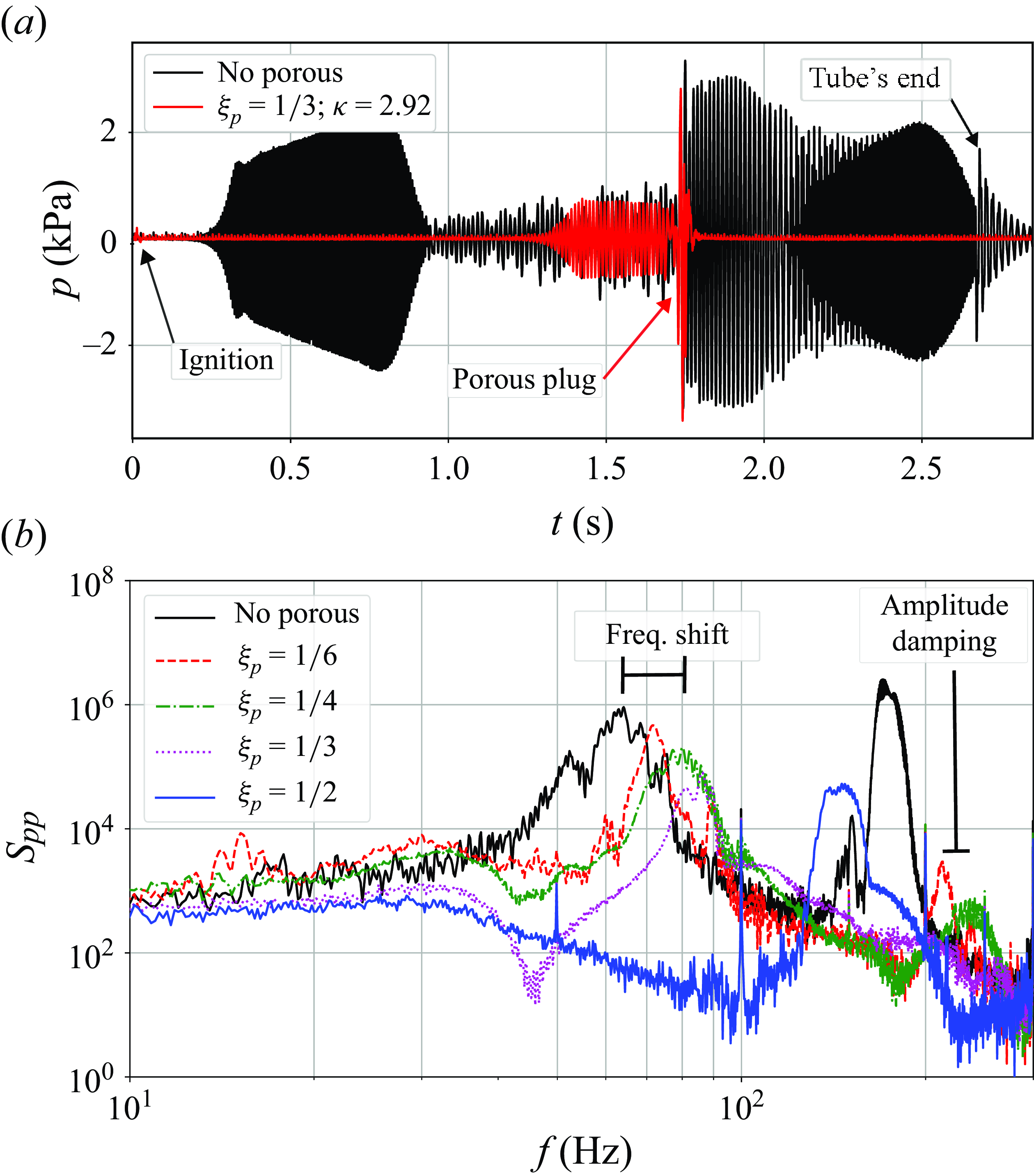
Regarding the frequencies, figure 11(a) presents the comparison of pressure signals between two experimental runs without (black) and with (red) a porous plug at $\xi _p= 1/3$
. It can be noted that the flame oscillation is controlled, with no noticeable transition to large-amplitude oscillations, with estimated porous properties that yield a value
$\xi _p= 1/3$
. It can be noted that the flame oscillation is controlled, with no noticeable transition to large-amplitude oscillations, with estimated porous properties that yield a value $\kappa = 2.92$
. Figure 11(b) shows the frequency spectra of the experimental pressure signals for a porous plug of dimensionless parameter
$\kappa = 2.92$
. Figure 11(b) shows the frequency spectra of the experimental pressure signals for a porous plug of dimensionless parameter $\kappa =2.92$
positioned at different
$\kappa =2.92$
positioned at different $\xi _p$
. The pressure data in the absence of the porous plug inside the pipe has been included (solid black). Two distinct frequency peaks are noticeable in this figure, corresponding to the fundamental mode and the first-harmonic mode. The fundamental frequency can be easily approximated in an open–closed tube as
$\xi _p$
. The pressure data in the absence of the porous plug inside the pipe has been included (solid black). Two distinct frequency peaks are noticeable in this figure, corresponding to the fundamental mode and the first-harmonic mode. The fundamental frequency can be easily approximated in an open–closed tube as $f_0 = {c_u}/{4 L}$
, given that the equivalent sinusoidal eigenfunction for isothermal acoustics exhibits a span quarter-wavelength, while the first harmonic is given by
$f_0 = {c_u}/{4 L}$
, given that the equivalent sinusoidal eigenfunction for isothermal acoustics exhibits a span quarter-wavelength, while the first harmonic is given by $f_1 = 3 c_u/4 L$
. In the case under examination, the fundamental frequency derived from the experimental data is approximately
$f_1 = 3 c_u/4 L$
. In the case under examination, the fundamental frequency derived from the experimental data is approximately $64\,\textrm{Hz}$
, higher than the approximate theoretical value of
$64\,\textrm{Hz}$
, higher than the approximate theoretical value of $53\,\textrm{Hz}$
, with
$53\,\textrm{Hz}$
, with $c_u =343\,\textrm{m s}^{-1}$
. Furthermore, as illustrated in figure 11(b), the introduction of the porous plug results in a reduction in power spectral density (
$c_u =343\,\textrm{m s}^{-1}$
. Furthermore, as illustrated in figure 11(b), the introduction of the porous plug results in a reduction in power spectral density ( $S_{pp}$
), accompanied by a shift in the peak frequency as the porous plug approaches the open end. The spectrum of each part of the pressure signal is computed as the product of the Fourier transform of the pressure
$S_{pp}$
), accompanied by a shift in the peak frequency as the porous plug approaches the open end. The spectrum of each part of the pressure signal is computed as the product of the Fourier transform of the pressure $\mathscr{F}[p]=\tilde {p}$
by its complex conjugate
$\mathscr{F}[p]=\tilde {p}$
by its complex conjugate $\tilde {p}^*$
:
$\tilde {p}^*$
: $S_{pp} = \tilde {p} \circ {\tilde {p}^*}$
.
$S_{pp} = \tilde {p} \circ {\tilde {p}^*}$
.
(a) Pressure signal evolution with time for a tube without (black) and with (red) a porous structure of $\kappa = 2.92$
at
$\kappa = 2.92$
at $\xi _p=1/3$
. (b) Power spectral density for a slender tube with a length of 160 cm and a porous plug with
$\xi _p=1/3$
. (b) Power spectral density for a slender tube with a length of 160 cm and a porous plug with $\kappa =2.92$
at different positions along the tube.
$\kappa =2.92$
at different positions along the tube.
Furthermore, the outcomes of the pressure sensor measurements are collated from a series of experiments in which the non-dimensional porous plug position, $\xi _p = L_p/L$
, is varied along the tube. In fact, figure 12 illustrates the pressure signal and spectrogram as a function of the flame location,
$\xi _p = L_p/L$
, is varied along the tube. In fact, figure 12 illustrates the pressure signal and spectrogram as a function of the flame location, $\xi _f$
, considering three positions of porous plugs,
$\xi _f$
, considering three positions of porous plugs, $\xi _p=$
1/6 (panels a,b), 1/3 (panels c,d) and 1/2 (panels e,f), respectively. The figures present the pressure signals as a function of the flame position. These are translated from the temporal measurements of pressure to spatial reconstruction, assuming a constant mean propagation velocity. Then, pressure signals and their spectrograms are represented with respect to the flame location,
$\xi _p=$
1/6 (panels a,b), 1/3 (panels c,d) and 1/2 (panels e,f), respectively. The figures present the pressure signals as a function of the flame position. These are translated from the temporal measurements of pressure to spatial reconstruction, assuming a constant mean propagation velocity. Then, pressure signals and their spectrograms are represented with respect to the flame location, $\xi _f=x_f/L$
, where
$\xi _f=x_f/L$
, where $x_f$
corresponds to the distance between the flame front and the closed end of the tube. Moreover, each panel in figure 12 represents a specific porous plug with a given value of permeability parameter
$x_f$
corresponds to the distance between the flame front and the closed end of the tube. Moreover, each panel in figure 12 represents a specific porous plug with a given value of permeability parameter $\kappa = 0.30$
(panels a,c,e) and
$\kappa = 0.30$
(panels a,c,e) and $\kappa =2.92$
(panels b,d,f).
$\kappa =2.92$
(panels b,d,f).
Pressure signal and spectrogram as a function of the flame position $\xi _f$
for various plug positions
$\xi _f$
for various plug positions $\xi _p =1/6$
(a,b),
$\xi _p =1/6$
(a,b), $\xi _p=1/3$
(c,d) and
$\xi _p=1/3$
(c,d) and $\xi _p = 1/2$
(e,f) and different porous properties
$\xi _p = 1/2$
(e,f) and different porous properties $\kappa = 0.3$
(a,c,e) and
$\kappa = 0.3$
(a,c,e) and $\kappa = 2.92$
(b,d,f). The model prediction (symbols) includes frequency responses and the dissipation
$\kappa = 2.92$
(b,d,f). The model prediction (symbols) includes frequency responses and the dissipation $\Omega _i$
(colourbar).
$\Omega _i$
(colourbar).
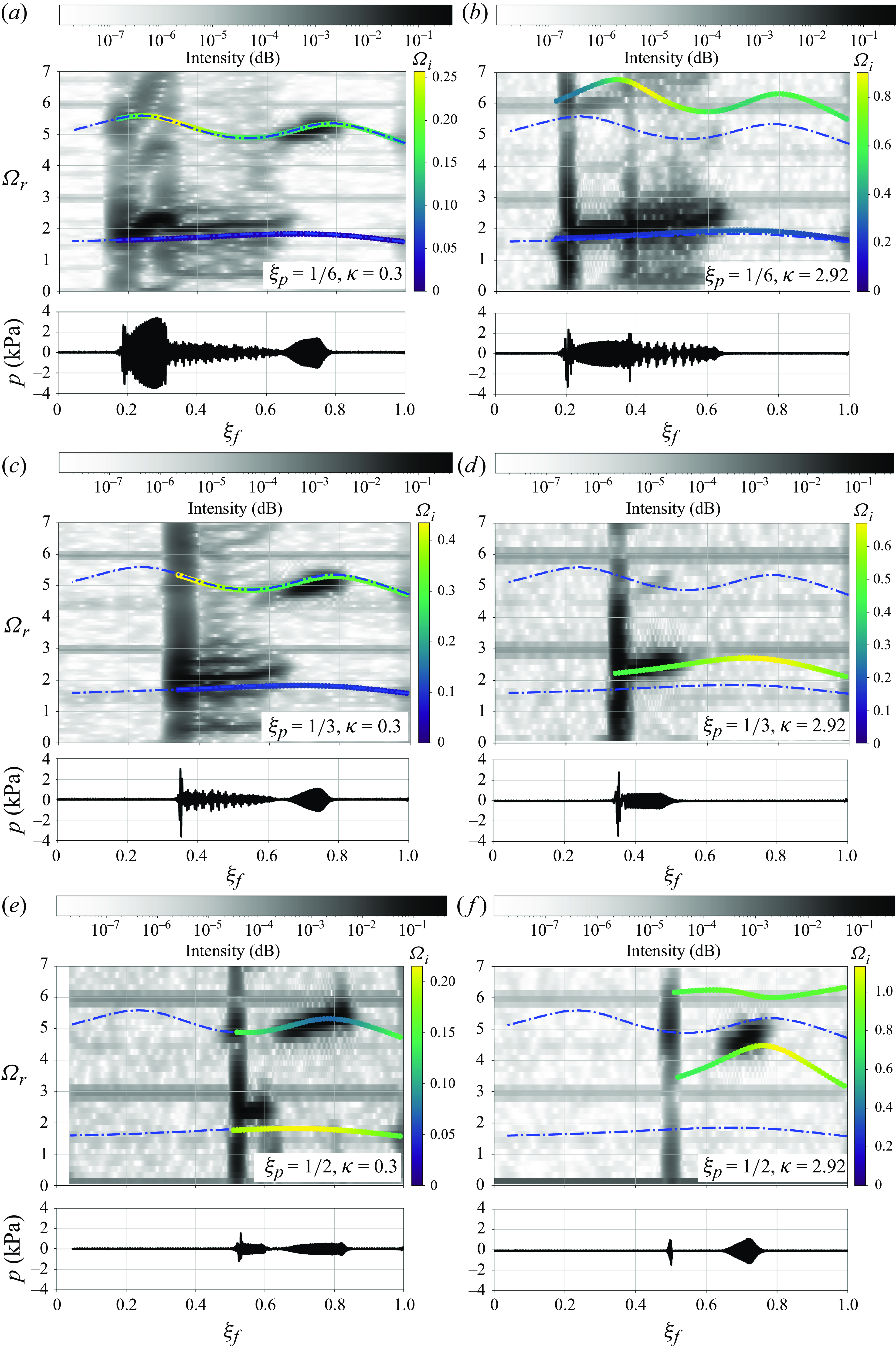
Additionally, the solutions obtained with the theoretical model proposed in this study have been included in the spectrogram with colour symbols, encompassing both the frequencies and the dissipation capacity (colourmap). In turn, the most dissipative flame positions (yellow symbols) are not excited in the experimental spectrogram (dark areas). Nevertheless, all the frequencies of experimentally self-excited regions show a great agreement with the theoretical frequency prediction. Also, it can be observed that as the porous plug becomes denser (higher $\kappa$
values) and is positioned closer to the open end (increasing
$\kappa$
values) and is positioned closer to the open end (increasing $\xi _p$
), the frequencies increase. This behaviour is more evident in the first harmonic, where the least dense porous plug generates a frequency change of approximately 5 %, and the frequency of the most dense increases up to 35 %. This behaviour can be attributed to the fact that as the density of the porous plug increases, the acoustic problem begins to behave like a wall of decreasing permeabilities, resulting in higher frequencies corresponding to shorter tubes. The prediction for the natural frequencies of the porousless model with heat losses in a tube length of 160 cm has been included (dot-dashed blue) for comparison, showing a lack of agreement as the porous parameter is increased. Finally, the spectrograms show the presence of spurious frequencies at specific values of
$\xi _p$
), the frequencies increase. This behaviour is more evident in the first harmonic, where the least dense porous plug generates a frequency change of approximately 5 %, and the frequency of the most dense increases up to 35 %. This behaviour can be attributed to the fact that as the density of the porous plug increases, the acoustic problem begins to behave like a wall of decreasing permeabilities, resulting in higher frequencies corresponding to shorter tubes. The prediction for the natural frequencies of the porousless model with heat losses in a tube length of 160 cm has been included (dot-dashed blue) for comparison, showing a lack of agreement as the porous parameter is increased. Finally, the spectrograms show the presence of spurious frequencies at specific values of $\Omega \approx 3$
(and its multiples), which correspond to frequencies of approximately 100 Hz associated with measurement equipment.
$\Omega \approx 3$
(and its multiples), which correspond to frequencies of approximately 100 Hz associated with measurement equipment.
The normalised spectrum $S_{pp}$
of the first (a) and second (b) spectrum peaks as a function of the porous plug position for different porous properties
$S_{pp}$
of the first (a) and second (b) spectrum peaks as a function of the porous plug position for different porous properties $\kappa$
.
$\kappa$
.
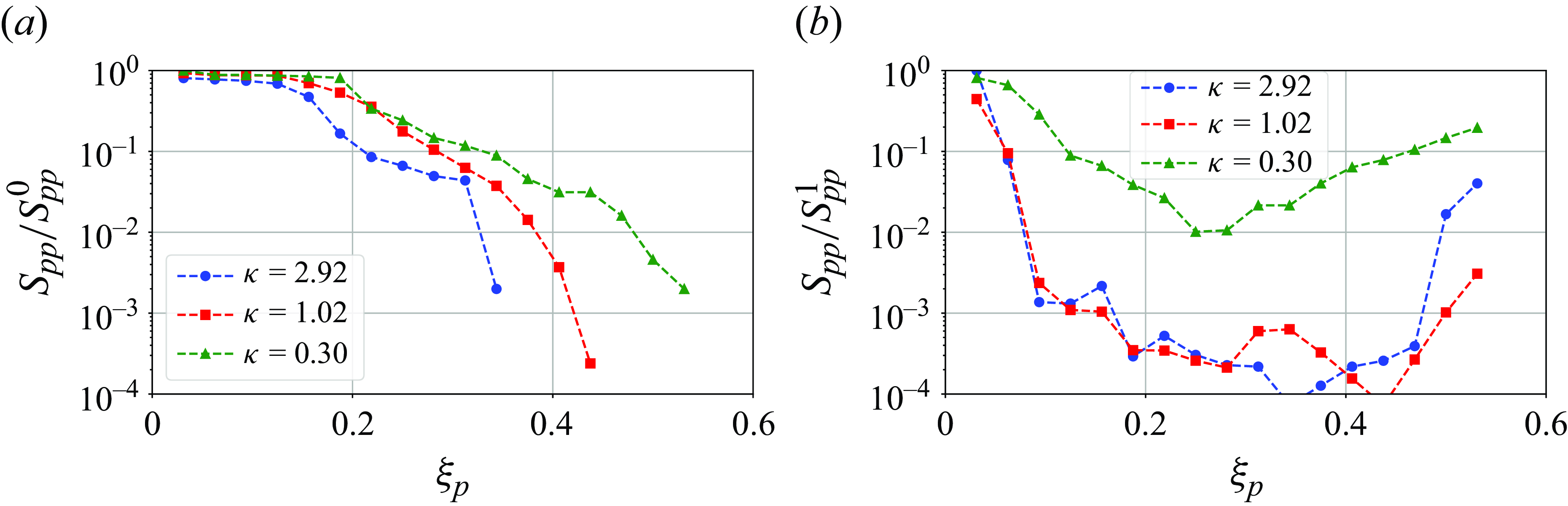
Next, a global measure of the decay of the excited frequencies, based on the position of the porous plug, is provided in figure 13. There, the amplitude of the power spectral density, denoted by $S_{pp}$
, normalised with respect to the porousless case is represented as a function of the porous plug position
$S_{pp}$
, normalised with respect to the porousless case is represented as a function of the porous plug position $\xi _p$
for the first (panel a) and second (panel b) frequency peaks. The spectrum values have been normalised respectively with respect to the amplitude of the fundamental mode’s peak in the spectrum,
$\xi _p$
for the first (panel a) and second (panel b) frequency peaks. The spectrum values have been normalised respectively with respect to the amplitude of the fundamental mode’s peak in the spectrum, $S_{pp}^0$
, and the first-harmonic mode’s peak,
$S_{pp}^0$
, and the first-harmonic mode’s peak, $S_{pp}^1$
, in the absence of the porous plug. As illustrated in figure 13(a), the dissipation efficiency of the porous plug appears to increase as the plug is displaced from the closed end of the slender tube. With regard to the first harmonic, the structure dissipates a greater quantity of energy at approximately one-third of the tube length, which is the approximate location of the pressure node of the first-harmonic mode, or velocity maximum where dissipation can be the greatest.
$S_{pp}^1$
, in the absence of the porous plug. As illustrated in figure 13(a), the dissipation efficiency of the porous plug appears to increase as the plug is displaced from the closed end of the slender tube. With regard to the first harmonic, the structure dissipates a greater quantity of energy at approximately one-third of the tube length, which is the approximate location of the pressure node of the first-harmonic mode, or velocity maximum where dissipation can be the greatest.
This information can also be extracted in an approximate manner from the theoretical model. Given the position of the porous dissipator, the frequencies as the flame position advances inside the tube can be predicted. The mean values of the imaginary part of the eigenvalues of the flame propagating inside the tube for each plug position $\xi _p$
are represented in figure 14. Here, a position-averaged damping factor is obtained which provides a qualitative agreement with the spectral power density decay in the experimental data in figure 13. However, it should be noted that when averaging the theoretical damping, all the flame positions with the local value of
$\xi _p$
are represented in figure 14. Here, a position-averaged damping factor is obtained which provides a qualitative agreement with the spectral power density decay in the experimental data in figure 13. However, it should be noted that when averaging the theoretical damping, all the flame positions with the local value of $\Omega _i$
are equally relevant, although in real experiments the amplitude of the oscillations varies among different regions of the tube, (figure 12
a,b). In any case, the experimental results cannot be compared directly with the model’s because they are essentially different; the experiments show amplitude deficit compared with the porousless case, instead of linear damping. It is useful to present the model’s damping
$\Omega _i$
are equally relevant, although in real experiments the amplitude of the oscillations varies among different regions of the tube, (figure 12
a,b). In any case, the experimental results cannot be compared directly with the model’s because they are essentially different; the experiments show amplitude deficit compared with the porousless case, instead of linear damping. It is useful to present the model’s damping $\Omega _i$
as
$\Omega _i$
as $e^{-\Omega _i}$
so as to represent it in the form of how the energy would decrease under linear damping. In any case, in figure 14, a band of uncertainty is shown around the averaged values whose limits correspond to the extreme values of the damping for all the flame positions. Its thinness indicates that the flame location in the tube is of little significance compared with the porous plug location.
$e^{-\Omega _i}$
so as to represent it in the form of how the energy would decrease under linear damping. In any case, in figure 14, a band of uncertainty is shown around the averaged values whose limits correspond to the extreme values of the damping for all the flame positions. Its thinness indicates that the flame location in the tube is of little significance compared with the porous plug location.
Theoretical damping $e^{-\bar {\Omega }_i}$
as a function of
$e^{-\bar {\Omega }_i}$
as a function of $\xi _p$
, averaged across all flame locations for the fundamental (a) and first-harmonic (b) modes and various
$\xi _p$
, averaged across all flame locations for the fundamental (a) and first-harmonic (b) modes and various $\kappa$
values.
$\kappa$
values.
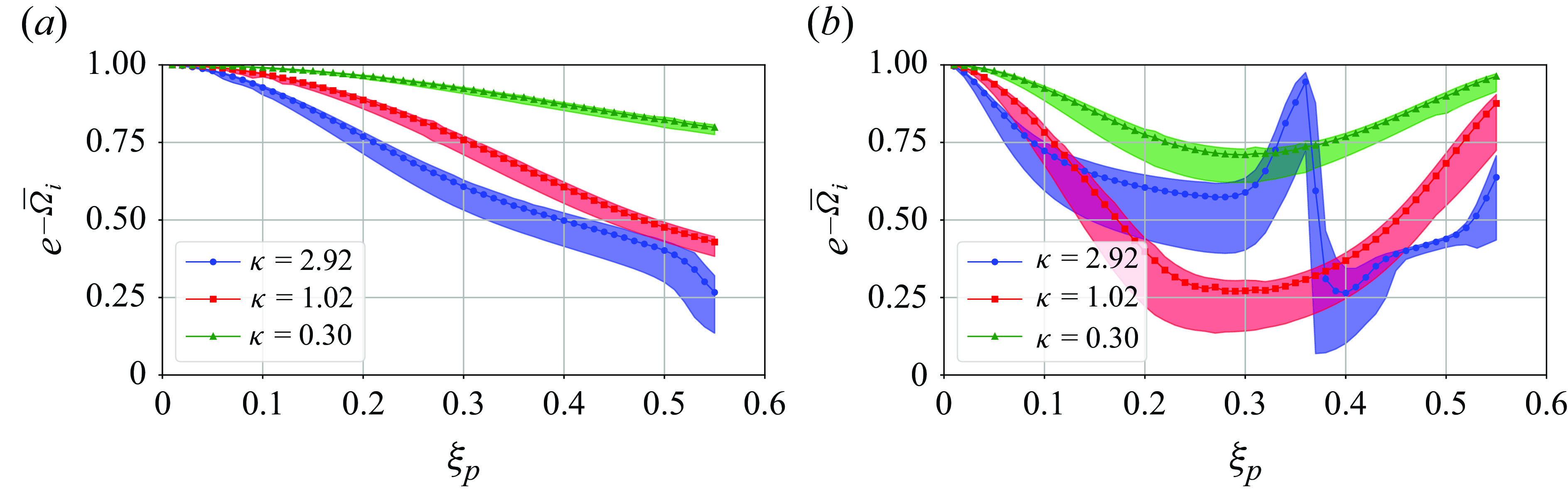
4.2. High-speed video data
The experimental tests were also recorded with the high-speed camera presented earlier, and the aforementioned image analysis was conducted to detect the contour of the flame front and centroid for each frame. The data processing enables the computation of the instantaneous flame velocity in each experiment by applying centred finite differences. As the velocity variable of the oscillatory motion is a function of time, the average value and standard deviation (calculated as the deviation of all data points with respect to the average propagation velocity) at each experimental configuration is discussed next.
Figure 15(a) presents the averaged flame propagation velocity, as a function of the porous plug parameter $\kappa$
and position at the tube
$\kappa$
and position at the tube $\xi _p$
. The value is normalised with respect to the averaged velocity in the absence of a porous plug within the tube (
$\xi _p$
. The value is normalised with respect to the averaged velocity in the absence of a porous plug within the tube ( $\overline {u}_0=0.552\,\textrm{m s}^-{^1})$
. These results illustrate that as the porosity
$\overline {u}_0=0.552\,\textrm{m s}^-{^1})$
. These results illustrate that as the porosity $\Phi$
decreases, smaller unit cell
$\Phi$
decreases, smaller unit cell $a$
, lower permeability
$a$
, lower permeability $K$
or greater porous parameter
$K$
or greater porous parameter $\kappa$
, the mean flame velocity also increases. In fact, the mean velocity is observed to increase by up to 10 % in comparison with the mean velocity in the absence of the porous plug. In figure 15(b), the normalised velocity standard deviation,
$\kappa$
, the mean flame velocity also increases. In fact, the mean velocity is observed to increase by up to 10 % in comparison with the mean velocity in the absence of the porous plug. In figure 15(b), the normalised velocity standard deviation, $SD$
, is presented as an indicator of the flame’s instability level in relation to the position of the porous plug. The
$SD$
, is presented as an indicator of the flame’s instability level in relation to the position of the porous plug. The $SD$
values have been normalised with respect to the standard deviation of the tube in the absence of the porous plug (
$SD$
values have been normalised with respect to the standard deviation of the tube in the absence of the porous plug ( $SD_0$
= 0.676 m s–1). Oscillations in flame-front velocities are directly associated directly with combustion instability issues, with higher
$SD_0$
= 0.676 m s–1). Oscillations in flame-front velocities are directly associated directly with combustion instability issues, with higher $SD$
showing greater instability. It can be observed that instabilities are lower when the porous plug is located around one-third of the tube length. Additionally, a direct relationship between pressure readings and image analysis can be observed when comparing the results from figures 15 and 13, showing consistent trends. Furthermore, an increase in the
$SD$
showing greater instability. It can be observed that instabilities are lower when the porous plug is located around one-third of the tube length. Additionally, a direct relationship between pressure readings and image analysis can be observed when comparing the results from figures 15 and 13, showing consistent trends. Furthermore, an increase in the $SD$
is accompanied by a decrease in the mean velocity. This finding is consistent with the results of previous studies on flames propagating under primary regime conditions (Flores-Montoya et al. Reference Flores-Montoya, Muntean, Pozo-Estivariz and Martínez-Ruiz2023), where the retracting period of the oscillating dynamics and the reduction in period-averaged flame surface produce a noticeable decay in overall flame propagation speed.
$SD$
is accompanied by a decrease in the mean velocity. This finding is consistent with the results of previous studies on flames propagating under primary regime conditions (Flores-Montoya et al. Reference Flores-Montoya, Muntean, Pozo-Estivariz and Martínez-Ruiz2023), where the retracting period of the oscillating dynamics and the reduction in period-averaged flame surface produce a noticeable decay in overall flame propagation speed.
Normalised mean flame velocity (a), and standard deviation as a function of the porous plug position (b).
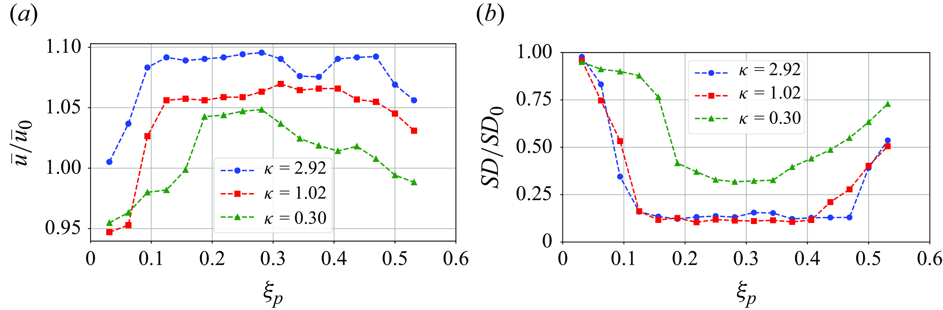
5. Summary and concluding remarks
The objective of this study was to conduct an experimental investigation into the efficacy of a porous plug in mitigating thermoacoustic waves associated with the propagation of a flame in a slender tube with a premixed air and methane mixture. The porous plugs were constructed using a lattice structure and were manufactured via additive 3-D printing. This study considered various porous plugs with varying porosity percentages. First, some characterisation tests were carried out to ascertain the properties of the porous plugs. A linear fit of the permeability coefficient was conducted for each configuration. Finally, the dissipation capacity of the porous plug was evaluated based on its position within the tube and its impact on the natural frequencies of flame propagation. To assess the efficacy of the porous plug, pressure readings and video analysis were conducted at high speeds.
Furthermore, a theoretical one-dimensional acoustic model was developed to estimate the variation in the natural frequencies of flame propagation and the capacity of the porous media to dissipate waves based on the position of the porous medium. Great agreement was achieved through the characterisation of the porous plug properties through parameter $\kappa$
. It was determined that the linear model aligns with the theoretical model in accordance with the experimental results. In fact, the incorporation of porous media with a high relative density results in a greater change in the natural frequencies of flame propagation, acting as a piston that alters the length of the tube. The theoretical model proposed in this work allows for the accurate prediction of acoustic frequencies and the qualitative estimation of the capacity of porous plugs to dissipate thermoacoustic waves based on their location and permeability.
$\kappa$
. It was determined that the linear model aligns with the theoretical model in accordance with the experimental results. In fact, the incorporation of porous media with a high relative density results in a greater change in the natural frequencies of flame propagation, acting as a piston that alters the length of the tube. The theoretical model proposed in this work allows for the accurate prediction of acoustic frequencies and the qualitative estimation of the capacity of porous plugs to dissipate thermoacoustic waves based on their location and permeability.
All things considered, porous materials may serve as a control mechanism for thermoacoustic instabilities, capable of dissipating up to $80\,\%$
of the energy generated through fundamental and first-harmonic modes in tubes. The precise location of the porous plug within the tube is of critical importance for the optimal mitigation of thermoacoustic waves. The most efficient location for the incorporation of porous plugs is approximately one-third of the length of the tube, where the pressure node and the maximum velocities of the first harmonic are located. This fact indicates that the mitigation mechanism of the porous plugs is based on viscous dissipation. This phenomenon is particularly evident in porous plugs with the lowest permeability. The conclusion is that this strategy can be employed and optimised as a chamber-based approach, considering the placement and design of the plugs, not an operational approach targeting specific modes and frequencies.
$80\,\%$
of the energy generated through fundamental and first-harmonic modes in tubes. The precise location of the porous plug within the tube is of critical importance for the optimal mitigation of thermoacoustic waves. The most efficient location for the incorporation of porous plugs is approximately one-third of the length of the tube, where the pressure node and the maximum velocities of the first harmonic are located. This fact indicates that the mitigation mechanism of the porous plugs is based on viscous dissipation. This phenomenon is particularly evident in porous plugs with the lowest permeability. The conclusion is that this strategy can be employed and optimised as a chamber-based approach, considering the placement and design of the plugs, not an operational approach targeting specific modes and frequencies.
Notwithstanding the aforementioned advantages of porous plugs in comparison with other solutions, such as Helmholtz resonators, there are several issues that limit their range of applicability. The long-term usage of porous plugs can be compromised by the accumulation of dirt particles that may clog the pores, and there is a risk of mechanical failure of the thin, porous walls under harsh conditions. Additionally, when deployed in devices with high mass flow rates, porous plugs may cause additional head losses if the bulk flow is forced through. Furthermore, the efficacy of the system is expected to decrease for frequencies much higher than those presented in this work, as the wavelengths could approach the length of the pores, thereby reducing the plug’s ability to attenuate acoustic waves. Therefore, a great design effort that grants further studies must be addressed in the case of considering sufficient advantages to apply these configurations to combustion systems.
A primary limitation of employing the porous plug as a means of mitigating combustion instability is that the flame does not traverse it. Therefore, our experimental set-up may be taken as a sort of cavity. Nevertheless, this is not the case in the sense of prescribing the reduction of one particular frequency through the design and size of the cavity, with a consistent damping of all the acoustic modes. Future experimental research will entail the incorporation of a hole in the porous plugs to permit the flame to pass through them, enabling the propagation in the closed part of the tube.
Acknowledgements
The authors would like to thank J.M. Velasco and A. Lloret del Blanco for their technical support in the construction of the experimental set-up.
Funding
This work was funded by the Regional Government of Madrid and by MCIN of Spain with funding from the European Union NextGenerationEU (PRTR-C17.I1) and through project TED2021-129446B-C43 funded by MCIN/AEI/ 10.13039/ 501100011033.
Declaration of interests
The authors report no conflict of interest.
Data availability statement
The data supporting this study’s findings are available from the corresponding author upon reasonable request.
Author contributions
Conceptualisation and methodology, P.G.P., M.B., V.M. and D.M.R.; software and validation, P.G.P. and M.B.; formal analysis, P.G.P., M.B. and D.M.R.; investigation, P.G.P., M.B., V.M. and D.M.R.; writing – original draft preparation, P.G.P., M.B. and D.M.R.; writing – review and editing, P.G.P., M.B., S.P.C., V.M. and D.M.R.; visualisation, P.G.P., M.B.; supervision, D.M.R.; project administration, resources and funding acquisition, D.M.R. and V.M.


 Open access