


1. Introduction
Roughness characterizes a plethora of turbulent flows at various scales – from the smallest scales encountered in geophysical flow (such as the roughness of individual surfaces, tree leaves, etc.) via the bulk roughness of real surfaces to the largest scales in the Earth system, where topographic undulations present a roughness for synoptic-scale systems. While under strong conditions on the surface properties, a flow can be considered hydraulically smooth (Pope Reference Pope2000), atmospheric flows are virtually always rough due to the small-scale heterogeneity of the underlying Earth's surface in combination with the low viscosity of air. The atmospheric boundary layer (ABL) is the lowest part of the Earth's atmosphere with a thickness of  $0.1$ to $2$ km (Garratt Reference Garratt1992) and a prototype rough ABL is the objective of this study.
Rotation of the Earth is a unique feature of the ABL; despite the small Rossby number, it causes significant departures in comparison with simpler canonical flows (e.g. closed channel or pipe flow). It is commonly considered by background rotation around the vertical axis – giving rise to Ekman flow (Ekman Reference Ekman1905). For a statistical two-point description of the flow, such rotation breaks the symmetry in the spanwise direction. Near the ground, surface friction comes into play and decelerates the flow, and the mean wind rotates in favour of the pressure gradient force, forming the Ekman spiral. Given the friction velocity  $u_\tau$ and the Coriolis parameter f, the outer scale of the Ekman flow $\delta =u_\tau /f$, a scale for the boundary-layer thickness, forms as a consequence of shear growth and rotational suppression of the boundary layer; though unknown a priori, it is a constant for neutrally stratified flow and depends on the Reynolds number only – in stark contrast to spatially evolving boundary layers. Further, the turbulent boundary layer is complemented by an infinite reservoir of non-turbulent fluid aloft, which can be entrained into the boundary layer, causing departures of mean-flow statistics with respect to non-external canonical flows.
Direct numerical simulation (DNS) of Ekman flow is a viable model for ABL turbulence. Following the seminal work of Coleman, Ferziger & Spalart (Reference Coleman, Ferziger and Spalart1990), it was studied for hydraulically smooth configurations (Coleman Reference Coleman1999; Shingai & Kawamura Reference Shingai and Kawamura2004; Miyashita, Iwamoto & Kawamura Reference Miyashita, Iwamoto and Kawamura2006; Spalart, Coleman & Johnstone Reference Spalart, Coleman and Johnstone2008, Reference Spalart, Coleman and Johnstone2009; Ansorge & Mellado Reference Ansorge and Mellado2014, Reference Ansorge and Mellado2016; Deusebio et al. Reference Deusebio, Brethouwer, Schlatter and Lindborg2014; Shah & Bou-Zeid Reference Shah and Bou-Zeid2014; Ansorge Reference Ansorge2019). Considerations over non-smooth surfaces are scarce: to the authors’ knowledge, Lee, Gohari & Sarkar (Reference Lee, Gohari and Sarkar2020), who conduct DNS of the Ekman flow for sinusoidal surface topography under neutral and stable density stratification, is the only example. They investigate two-dimensional periodic bumps with  $H^+=15$ at $Re_\tau =700$, where $H^+$ is the height of the bumps in viscous units and $Re_\tau$ the friction Reynolds number, i.e. in the transitionally rough regime and find increased turbulent kinetic energy (TKE) production with an increasing slope of the bumps – counteracting buoyancy-induced suppression of turbulence. Limitations of the study are the absence of sharp edges, thus limiting flow instability and flow turbulence enhancement, the two-dimensional shape of their roughness elements and limited scale separation ( $Re_\tau$). Here, we complement this approach by (i) adding square surface elements to represent the small-scale roughness over homogeneous surfaces encountered frequently underneath the ABL and (ii) by an increased scale separation.
The effect of a rough boundary in turbulent flow is reviewed by Raupach, Antonia & Rajagopalan (Reference Raupach, Antonia and Rajagopalan1991), Finnigan (Reference Finnigan2000), Jiménez (Reference Jiménez2004), Kadivar, Tormey & McGranaghan (Reference Kadivar, Tormey and McGranaghan2021) and Chung et al. (Reference Chung, Hutchins, Schultz and Flack2021). Homogeneously rough flow, i.e. flow with a statistically homogeneous description of the roughness elements, is governed by two dimensionless parameters: (i) a roughness Reynolds number
 \begin{equation} H^+ = \frac{H}{\delta_\nu}, \end{equation}
where  $H$ is the height of roughness, $\delta _\nu =\nu /u_\tau$ the viscous length scale with $u_\tau$ the friction velocity and $\nu$ the kinematic viscosity, and (ii) the blocking ratio $H/\delta$, where $\delta$ is the boundary-layer thickness. Different roughness regimes are encountered for increasing $H^+$, ranging from hydraulically smooth – where no roughness effects are found in the flow statistics above the viscous layer – via transitionally rough to fully rough – where pressure drag outweighs the skin frictional drag and the buffer layer is replaced by a roughness sublayer. Values for the regime transitions are reported based on experiments (cf. table 2 in Kadivar et al. Reference Kadivar, Tormey and McGranaghan2021). These are based on the pioneering work of Nikuradse (Reference Nikuradse1933), who studied pipe flow with uniform sand-grain roughness and on the later work by Schlichting (Reference Schlichting1936), who introduced the equivalent sand-grain roughness with the aim of transferring Nikuradse's theory to other roughness geometries. In essence, the latter work suggests there exists an approximate scale $z_{0{m}}$ representing roughness effects also for less ideal configurations. This equivalent parameter, the aerodynamic roughness length for momentum $z_{0{m}}$, defines an empirical roughness Reynolds number $z_{0{m}}^+$ which is commonly used in studies of rough configurations. The ABL flow is considered hydraulically smooth flow for $z_{0{m}}^+ \lesssim 0.135$ and fully rough for $z_{0{m}}^+ \gtrsim 2-2.5$ with the transitionally rough regime in between (Brutsaert Reference Brutsaert1982; Andreas Reference Andreas1987). The zero-plane displacement height $d$ reflects a virtual shift of the effective underlying surface for high packing densities when fitting the logarithmic law. In the essence of classical scaling theory, the logarithmic law of the wall for the mean velocity $\bar {u}(z)$ under neutral conditions is
 \begin{equation} \bar{u}(z) = \frac{u_\tau}{\kappa}\ln \left(\frac{z}{z_0}\right), \end{equation}
following the notation of Monin (Reference Monin1970) (cf. their equation 9a), with the von Kármán constant  $\kappa$. For flow over rough surfaces, $z$ is substituted by $z-d$ (in 1.2), for consideration of the zero-plane displacement height $d$. This form of the logarithmic law – with the roughness parameter $z_0$ – forms the cornerstone of the Monin–Obukhov similarity theory (MOST, cf. Monin Reference Monin1970; Foken Reference Foken2006).
The second parameter of the roughness, the blocking ratio  $H/\delta$, can be used to describe the influence of roughness on the logarithmic layer and wall similarity (based on Townsend Reference Townsend1961, Reference Townsend1976, and elaborated by Raupach et al. Reference Raupach, Antonia and Rajagopalan1991). Jiménez (Reference Jiménez2004) found that wall similarity holds if $\delta /H > \delta _{crit}/H$ for $\delta _{crit}/H \approx 40\unicode{x2013}80$. Notably, for the friction Reynolds number $Re_\tau =\delta ^+$, it is
 \begin{equation} Re_\tau = \frac{\delta}{H} H^+ = \delta^+. \end{equation}
However, this suggests that the total turbulent scale separation measured in terms of  $Re_\tau$ is to be considered as geometrically composed of, first, a separation between large eddies and the roughness scale and, second, a separation between the roughness scale and viscosity. The scale separation between the inner viscous scale $\delta _{inner}$ and the outer scale $\delta _{outer}$ of the problem in a general formulation is given as
 \begin{equation} Re_{gen} = \frac{\delta_{outer}}{\delta_{inner}} = \frac{\delta}{F(\delta_\nu, H)}, \end{equation}
in the form of the general-Reynolds number  $Re_{gen}$. In the smooth limit, it is ${\delta _{inner}\sim \delta _\nu }$, $Re_{gen}$ is the friction Reynolds number $Re_\tau$. However, in the fully rough limit ${\delta _{inner}\sim H}$ and $Re_{gen}$ is the blockage ratio $\delta /H$. An overlap and logarithmic layer is only present if the scale separation in terms of $Re_{gen}$ is sufficiently large.
When interpreting turbulent Ekman flow as an idealized representation of the ABL, a DNS approach inevitably resorts to the concept of Reynolds-number similarity: the scale separation necessary for a direct representation of geophysical problems at scale is out of reach, even using the most modern computational approaches. The common representation of a prototype turbulent flow shows a cascade of motions from large-scale energy-containing eddies to the dissipation range (figure 1). If there is sufficient scale separation in between the two, the inertial range develops a self-similar scaling. In this regime of fully developed turbulence, i.e. when a sufficiently large inertial range exists (Dimotakis Reference Dimotakis2005), the spectral properties are well described by the seminal theory put forward by Kolmogorov (Reference Kolmogorov1941) and Obukhov (Reference Obukhov1941). Further, some statistics of the flow – in particular low-order statistics, such as dissipation (Dimotakis Reference Dimotakis2005) and mean velocity profiles (Barenblatt Reference Barenblatt1993) – will cease to depend on the separation of scales, viz. Reynolds number. While these scales, and thus also  $Re_\tau$, exist and bear a physical meaning in the rough configuration, the roughness parameter $L_r$ (characteristic roughness length scale) defines a new length scale. For all problems of relevance, it is $L\gg L_r$, with $L$ the scale of the largest eddies and in our specific problem we identify $L\sim {{O}}(\delta )$ with the boundary-layer thickness, and $L_r\gtrsim {{O}}(\delta _\nu )$ (if $L_r \ll \delta _\nu$, the surface must be aerodynamically smooth; and if $L_r$ reaches ${{O}}(\delta )$, an obstacle is no longer considered a roughness element). In analogy to the decomposition of the Reynolds number $Re_\tau$ proposed above (1.3), this gives rise to a roughness Reynolds number $Re_r\propto L_r/\delta _\nu$ which can be interpreted as a range of eddy sizes locally ‘occupied’ by roughness. This range is not available for an undisturbed continuation of the inertial range as roughness alters the scales of turbulent production, as measured by $u_\tau$, and local dissipation of turbulence kinetic energy (Davidson & Krogstad Reference Davidson and Krogstad2014). From the perspective of large-scale motions, this limitation is similar to reducing the Reynolds number by ${{O}}(Re_r^{-1})$. In our study we will hence resort to cases with $Re_r={{O}}(1)$ such that the turbulence instability of the large-scale eddies is retained despite the intermediate Reynolds number achieved in our DNS. While this limits us to relatively small roughness elements, we retain a proper turbulent interaction between the inner and outer scales as is observed in the real-world ABL.
Schematic of the scale separation in a turbulent flow as a function of the eddy sizes, with roughness acting at a range of scale  ${{O}}(L_r)$. The energy-containing eddies are ${{O}}(\delta )$ for a turbulent Ekman layer and the onset of the dissipation range is located at ${{O}}(\delta _\nu )$, with the viscous scale $\delta _\nu =\nu /u_\tau$. The Reynolds numbers $Re_{\tau }$ and $Re_r$ in this schematic give rise to a reduced Reynolds number $Re_{\tau } \propto Re_{\tau }/Re_r$, capturing the scale separation available for large-scale eddies until they hit the effects of bulk roughness.

The investigation of roughness gives rise to a huge parameter space, as the geometry, distribution and arrangement of roughness elements impact on the turbulent flow (Kadivar et al. Reference Kadivar, Tormey and McGranaghan2021). Cubical roughness elements are one preferred set-up for studying the effect of three-dimensional roughness on wall-bounded turbulent flow in vegetation and urban canopies, and we choose them also here as the building blocks of the rough surface. There are several numerical studies with staggered or aligned arrays, varying the roughness density and the size of roughness elements. The problem is investigated through DNS for channel flow (Coceal et al. Reference Coceal, Thomas, Castro and Belcher2006; Leonardi & Castro Reference Leonardi and Castro2010), and for a turbulent boundary layer (Lee, Sung & Krogstad Reference Lee, Sung and Krogstad2011b). It was also assessed by large-eddy simulation (LES) (Stoesser et al. Reference Stoesser, Mathey, Fröhlich and Rodi2003; Kanda, Moriwaki & Kasamatsu Reference Kanda, Moriwaki and Kasamatsu2004; Cheng & Porté-Agel Reference Cheng and Porté-Agel2015) and through wind tunnel measurements (Castro Reference Castro2007; Cheng et al. Reference Cheng, Hayden, Robins and Castro2007; Perret et al. Reference Perret, Basley, Mathis and Piquet2019). Coceal et al. (Reference Coceal, Thomas, Castro and Belcher2006) emphasize the difference between two- and three-dimensional roughness: mixing and transport are different for a two-dimensional setting. For flow orthogonal to the elements, there are unrealistically large sheltering effects; for flow parallel to elements, secondary motions become unrealistically large. Furthermore, their findings imply that a variable height of the roughness elements is needed to capture real-world conditions. Indeed, LES studies of Xie, Coceal & Castro (Reference Xie, Coceal and Castro2008) and Yang et al. (Reference Yang, Sadique, Mittal and Meneveau2016), investigated flows over blocks with a Gaussian height distribution. In this study, we chose blocks with a uniform height and width distribution to represent the randomness of individual roughness elements. Individual roughness elements are randomly offset from an equidistant, regular grid to also break symmetry due their positioning. The height of roughness elements can be considered with respect to the outer scale  $\delta$ (giving rise to the blocking ratio) and the inner scale $\nu /u_\tau$ (yielding the roughness Reynolds number $H^+$; cf. (1.3)). The present work is limited to rectangular roughness blocks with a small blocking ratio ( $H/\delta \lesssim 1.5\,\%$) such that sufficient scale separation exists for a logarithmic layer to form.
The packing density of roughness elements – and hence the mutual sheltering– gives rise to three different flow regimes: isolated roughness, wake interference and skimming flow (Hussain & Lee Reference Hussain and Lee1980; Grimmond & Oke Reference Grimmond and Oke1999). In the skimming regime, the packing density is sufficiently high such that the flow ‘slides’ over the roughness crests. In the other extreme case, the isolated roughness, the flow interaction between roughness elements is negligible and roughness elements can be considered as individual bluff bodies. Leonardi & Castro (Reference Leonardi and Castro2010) found the drag maximum for a packing density of  $15\,\%$, which is in agreement with Kanda et al. (Reference Kanda, Inagaki, Miyamoto, Gryschka and Raasch2013), whereas Ahn, Lee & Sung (Reference Ahn, Lee and Sung2013) measured a value of $11.1\,\%$ to $12.5\,\%$ and Cheng & Porté-Agel (Reference Cheng and Porté-Agel2015) a value of $~10\,\%$. In the present study, we use a packing density of approximately $10\,\%$, which falls in between isolated and wake interference roughness according to Grimmond & Oke (Reference Grimmond and Oke1999) (cf. their figure 1).
In the current work, we aim to answer the following research questions regarding the quantitative effects of surface roughness on a prototype ABL: (i) What is the impact of a controlled and fully resolved surface roughness on bulk parameters and mean flow properties in the inner and outer layer? (ii) Do the rough-wall scaling and log-layer scaling follow the expected and widely used approaches in MOST for neutral conditions? (iii) Can we arrive at meaningful estimates for the zero-plane displacement and roughness length for momentum and scalar? (iv) How different is the enhanced mixing of the momentum and of the scalar in the presence of surface roughness? To do so, we extend a well-established modelling set-up for turbulent Ekman flow by an immersed boundary method (IBM) and deploy the problem on the supercomputing system Hawk at Höchstleistungsrechenzentrum Stuttgart (HLRS, Germany) to reach scale separation of up to  $Re_\tau \approx 2700$.
2. Methodology
We consider Ekman flow of an incompressible fluid over a horizontal plate on the f-plane, that is, the Coriolis force only affects the horizontal velocity components and is constant. Far away from the wall, shear effects vanish and the flow is in geostrophic equilibrium, i.e. the pressure gradient is balanced by the Coriolis force.
2.1. Governing equations and parameters
The three-dimensional Navier–Stokes equations are numerically solved for an incompressible, Newtonian fluid with constant fluid properties (density  $\rho$, viscosity $\nu$) subject to steady system rotation about the vertical axis. The problem is discretized on the Cartesian coordinate system ${X_i=(X,Y,Z )^{\rm T}}$, where $X,Y$ is the streamwise, spanwise and $Z$ the wall-normal coordinate, and we solve it on a cubic domain of size ${[0,0,0]\leq [X,Y,Z]\leq [L_x,L_y,L_z]}$. The streamwise direction is defined with respect to the smooth-wall flow; the flow direction deviates with increasing height and surface roughness. The dynamical system is governed by the following parameters: (i) the geostrophic wind vector ${\boldsymbol {G}=(G_1,G_2,0)^{\rm T}}$ and force ${G=\sqrt {G_1^2 + G_2^2}}$, and (ii) the Coriolis parameter f. Both scales yield the Rossby radius ${\varLambda _{Ro} = G/f}$ as a length scale. Thus, the governing flow equations are non-dimensionalized with the characteristic scales $G, f,\ \varLambda _{Ro}$ and read
 \begin{equation} \frac{\partial u_i}{\partial x_i} = 0, \quad \frac{\partial u_i}{\partial t} + u_j\frac{\partial u_i}{\partial x_j} ={-}\frac{\partial {\rm \pi}}{\partial x_i} + \frac{1}{Re_\varLambda}\frac{\partial^2 u_i}{\partial x_j^2} + f\epsilon_{ik3}(u_k-g_k). \end{equation}
Here,  $t$ is the non-dimensional time, ${\boldsymbol {u}=(u,v,w)^{\rm T}}=(u_1,u_2,u_3)^{\rm T}$ is the non-dimensional velocity vector, ${x_i=(x,y,z)^{\rm T}}$ the non-dimensional coordinates and $\partial {\rm \pi}/\partial x_i$ the non-dimensional, non-hydrostatic, ageostrophic pressure gradient. Further, $\boldsymbol {g}=(g_1,g_2,0)^{\rm T}$ with $g_j=G_j/G$ is the normalized geostrophic wind (by construction ${g=\|\boldsymbol {g}\|=1}$) and $\epsilon _{ijk}$ is the alternating unit tensor. The boundary conditions for the velocities are no slip at the bottom and free slip at the top boundary; periodic boundary conditions are applied in the horizontal directions. Equations (2.1b) solely depend on the Reynolds number ${Re_{\varLambda }=\varLambda _{Ro}G/\nu }$. For comparison with other studies, we refer to the Reynolds number
 \begin{equation} Re_D = \frac{GD}{\nu}=\sqrt{2 Re_\varLambda}, \end{equation}
with  $D = \sqrt {2\nu f^{-1}}$ the laminar Ekman layer thickness. Both Rossby and Ekman scalings lose their relevance once the system is in a fully turbulent state. Then, the system is scaled by the friction velocity $u_\tau$ (non-dimensionalized form ${u_\star =u_\tau /G}$), the turbulent boundary-layer thickness ${\delta =u_\tau /f}$ (non-dimensionalized form ${\delta _\star =\delta /\varLambda _{Ro}=u_\star }$) and the eddy-turnover scale ${f^{-1}}$. These turbulent scales result in the friction Reynolds number $Re_\tau =u_\tau \delta /\nu$ with
 \begin{equation} u_\star^2 = \frac{1}{Re_\varLambda} \sqrt{ \left( \left.\frac{\partial \langle u \rangle }{\partial z}\right \rvert_{z=0} \right) ^2 + \left(\left. \frac{\partial \langle v \rangle}{\partial z}\right\rvert_{z=0} \right) ^2}, \end{equation}
such that  $Re_\tau$ equals the non-dimensional wind-speed gradient at the surface. The definition (2.3) of $u_\star$ is valid for a smooth wall located at ${z=0}$. Over a non-flat surface, it is ${u_\star ^2=\|\boldsymbol{\tau}_w\| /( \rho G^2)=\|\boldsymbol{\tau}_\star \| }$, where $\boldsymbol{\tau}_w$ is the total surface shear stress (non-dimensional form $\boldsymbol{\tau}_\star$) and $\rho$ the constant fluid density. As a consequence of rotation, the surface shear stress is not aligned with the geostrophic wind vector and the wind veers towards the surface as
 \begin{equation} \alpha(z) \sphericalangle(\langle\overline{\boldsymbol{u}}(z)\rangle ,\boldsymbol{g}) \quad \text{and} \quad \alpha_\star \sphericalangle(-\boldsymbol{\tau}_\star, \boldsymbol{g}). \end{equation}
The values  $u_\star$, $\alpha _\star$ and $\delta _\star$ are unknown a priori but can be approximated as functions of $Re_D$ (Spalart Reference Spalart1989). In external flow, there is a duality of scales, where the inner layer scales in inner units and the corresponding normalized quantities are denoted by $({\cdot })^+$, while the outer layer scales in outer units, denoted by $({\cdot })^-$. The non-dimensional length and velocity scales are defined as
 \begin{equation} x_i^+ = x_i u_\star Re_\varLambda = \frac{X_i}{\delta_\nu}, \quad u_i^+ = \frac{u_i}{u_\star}, \quad x_i^- = \frac{x_i}{u_\star} = \frac{X_i}{\delta}, \quad u_i^- = u_i. \end{equation}
The scalings are mapped by  ${x_i^+=Re_\tau x_i^-}$ and ${u_i^- = u_\star u_i^+}$. Spatial averaging of flow variables in the horizontal is denoted by ${\langle ({\cdot } ) \rangle }$ and temporal averaging by ${\overline {( {\cdot } )}}$.
Along with the conservation equation of momentum, we solve the transport equation of a passive scalar  $s$. Boundary conditions for the passive scalar are of Dirichlet type, with a constant difference between the lower and upper walls ${\Delta s=s|_{z=L_z} - s|_{z=w}}$, with ${s|_{z=L_z}=1}$ and ${s|_{z=w}=0}$. The conservation equation of the scalar is non-dimensionalized with the additional characteristic scale $\Delta s$, and it reads as
 \begin{equation} \frac{\partial s}{\partial t} + u_j\frac{\partial s}{\partial x_j} = \frac{1}{Re_\varLambda Sc}\frac{\partial^2 s}{\partial x_j^2}, \end{equation}
with
 \begin{equation} Sc=\frac{\nu}{\kappa_d}, \end{equation}
where  $Sc$ is the Schmidt number and $\kappa _d$ the constant molecular diffusivity for the scalar. Analogously to the friction velocity we define a non-dimensional reference friction value for the scalar with
 \begin{equation} s_\star = \frac{q_\star}{u_\star} \quad \text{and} \quad q_\star = \frac{1}{Re_\varLambda Sc} \left.\frac{\partial s}{\partial z}\right|_{z=0}, \end{equation}
where  $q_\star$ is the surface flux of the scalar for a smooth surface at $z=0$. The scalar in inner units is given by ${s^+=s/s_\star }$ and in outer units by ${s^-=s}$, since $s$ is scaled by $\Delta s$.
Following Ansorge (Reference Ansorge2017), a Rayleigh-damping layer is introduced on the uppermost 20 grid points to suppress spurious boundary effects, that may occur as a consequence of a finite domain height.
2.2. Intrinsic averaging
Intrinsic averaging implies that only values inside the fluid domain are considered for averaging, in contrast to extrinsic averaging, where all values in the whole domain are taken into account. Since there is a mismatch between the volume share covered by roughness elements (figure 2a, red and blue shaded area) and the corresponding share of grid points, a volume approach (figure 2b) yielding a fluid fraction for the volume in the box around each grid point is used and described in detail in Appendix A. In this study, we apply intrinsic averaging to all mean vertical profiles and global flow parameters, within the roughness layer  ${z\leq H_{max}}$, where $H_{max}$ is the height of the largest roughness element.
(a) Two-dimensional schematic of a solid object (red points) covering the area  $A^1$ immersed in a fluid domain (black points) covering the area $A^0$. The blue-shaded area belongs to the fluid, but field values in the area would be represented by the value on the solid surface. (b) Corresponding indicator field with volume fractions of the fluid ${\epsilon ^F(x_i )=[1- \epsilon ^S(x_i )]}$.

2.3. Numerical approach of the DNS code
Simulations in this study use the open source DNS code tlab (https://github.com/turbulencia/tlab). The governing equations are advanced in time with a fourth-order five-stage low-storage Runge–Kutta scheme (Williamson Reference Williamson1980). Spatial derivatives are computed with finite differences of sixth-order accuracy (Lele Reference Lele1992). Biased compact schemes of reduced order are used at the vertical (non-periodic) boundaries. The applied discretization results in an overall fourth-order accuracy of the code. Incompressibility is enforced with the fractional step method (Chorin Reference Chorin1968; Témam Reference Témam1969) to ensure divergence-free velocity fields up to machine accuracy. The Poisson solver uses a Fourier-spectral approach in the periodic horizontal directions, and an inverse-compact approach along the vertical (Mellado & Ansorge Reference Mellado and Ansorge2012). Originally, pressure and velocities are computed on the same grid in tlab. This collocated arrangement is well known to cause spurious pressure oscillations (Laizet & Lamballais Reference Laizet and Lamballais2009) in combination with an IBM. Hence, the existing code was extended by a partially staggered pressure grid in the horizontal and a compact filter (Lele Reference Lele1992) for the pressure in the vertical to circumvent the deterioration of the data by numerical artefacts in the pressure.
2.4. Immersed boundary method
The representation of flow obstacles with vertical walls and rigid boundaries challenges DNS codes of high-order accuracy and may cause numerical artefacts, referred to as spurious force oscillations (SFOs). With the aim of using Cartesian grids, an IBM is implemented in tlab and tested against reference data to ensure sufficient resolution and absence of SFOs that deteriorate the flow statistics.
The Gibbs phenomenon and SFOs are known artefacts to occur in moving-body problems (Lee et al. Reference Lee, Kim, Choi and Yang2011a), but also for non-moving bodies represented through an IBM (Li, Bou-Zeid & Anderson Reference Li, Bou-Zeid and Anderson2016). The SFOs appear as high-frequency oscillations near a solid boundary (Fornberg Reference Fornberg1996, p. 11). They can severely deteriorate the numerical solution. Not only may this impact instantaneous realizations of the flow, but also the long-time averages of flow quantities. In our case of rigid bodies represented by an IBM, SFOs are caused by a stepwise signal of the IBM forcing at the solid boundary in combination with a spectral-like compact differencing scheme. The oscillations may contaminate the flow field due to the non-local character of these schemes. Filtering and smoothing procedures in physical and frequency space can be used to reduce or control SFOs (Goldstein, Handler & Sirovich Reference Goldstein, Handler and Sirovich1993; Kim, Kim & Choi Reference Kim, Kim and Choi2001; Lamballais & Silvestrini Reference Lamballais and Silvestrini2002; Tseng, Meneveau & Parlange Reference Tseng, Meneveau and Parlange2006; Fang et al. Reference Fang, Diebold, Higgins and Parlange2011).
The direct forcing IBM approach was introduced by Mohd-Yusof (Reference Mohd-Yusof1997) and Fadlun et al. (Reference Fadlun, Verzicco, Orlandi and Mohd-Yusof2000). It tries to avoid SFOs through an artificial flow in the solid regions that reduces discontinuities at the interface while fulfilling the boundary conditions. This leaves the external flow unaffected by the artificial flow (Fadlun et al. Reference Fadlun, Verzicco, Orlandi and Mohd-Yusof2000). While the method was extended towards higher-order derivative schemes (Parnaudeau et al. Reference Parnaudeau, Lamballais, Heitz, Silvestrini, Friedrich, Geurts and Métais2004, Reference Parnaudeau, Carlier, Heitz and Lamballais2008), it remains limited to simple geometries like cylinders, and is problematic for objects with sharp edges (Giannenas & Laizet Reference Giannenas and Laizet2021, figure 2 on p. 610).
The alternating direction reconstruction (ADR) IBM, proposed by Gautier, Laizet & Lamballais (Reference Gautier, Laizet and Lamballais2014), allows simulations with more complex geometries while preserving the homogeneity of spatial operators. The flow is artificially expanded into solid regions to ensure the smoothness of fields across the interface, while the boundary conditions  ${u_i |_{interface}=0}$ are met. Gautier et al. (Reference Gautier, Laizet and Lamballais2014) used one-dimensional Lagrangian polynomials for interpolation, which are evaluated in the respective direction before a spatial derivative of the governing equations is evaluated in this direction. This procedure is repeated anew for each derivative and the values within the solid regions are not considered for subsequent calculations.
Lagrangian polynomials suffer from Runge's phenomenon (Runge Reference Runge1901), where large amplitudes occur at the boundaries for equidistant grids. As objects get wider, numerical instabilities can occur due to unphysically large derivatives at the interface and corresponding large pressure signals inside the solid. Giannenas & Laizet (Reference Giannenas and Laizet2021) use cubic splines, avoiding the Runge phenomenon at boundary nodes, which results in reduced amplitudes of the auxiliary field within the solid. They demonstrate that the ADR IBM with cubic splines is well suited for sixth-order compact schemes and does not degrade the overall convergence order of the DNS code. Further, no additional stability constraints emerge and the computational overhead is marginal. Finally, the ADR IBM is highly scalable on high-performance computing systems, as the communication overhead of the parallel algorithm does not increase.
The ADR IBM is well tested for flow around a cylinder against both experimental and simulation data (Parnaudeau et al. Reference Parnaudeau, Carlier, Heitz and Lamballais2008; Gautier, Biau & Lamballais Reference Gautier, Biau and Lamballais2013; Gautier et al. Reference Gautier, Laizet and Lamballais2014; Giannenas & Laizet Reference Giannenas and Laizet2021) and across different DNS codes (Schäfer et al. Reference Schäfer, Forooghi, Straub, Frohnapfel, Stroh, García-Villalba, Kuerten and Salvetti2020; Theobald et al. Reference Theobald, Schäfer, Yang, Frohnapfel, Stripf, Forooghi and Stroh2021). More recently, the ADR IBM was also applied for moving objects (Giannenas & Laizet Reference Giannenas and Laizet2021), to wavy channel turbulence (Khan & Jayaraman Reference Khan and Jayaraman2019; Jayaraman & Khan Reference Jayaraman and Khan2020), jet control with microjets (Gautier et al. Reference Gautier, Laizet and Lamballais2014), LES of a circular cylinder wake flow (Resseguier et al. Reference Resseguier, Mémin, Heitz and Chapron2017; Chandramouli et al. Reference Chandramouli, Heitz, Laizet and Mémin2018), flow over periodic hill (Xiao et al. Reference Xiao, Wu, Laizet and Duan2020) and to channel flow over streamwise-aligned ridges (Schäfer et al. Reference Schäfer, Stroh, Frohnapfel and Gatti2019) and with free convection (Schäfer et al. Reference Schäfer, Stroh, Forooghi and Frohnapfel2022b).
The implementation of the ADR IBM based on cubic splines in tlab enables DNS of Ekman flow with fully resolved roughness. An indicator field  $\epsilon (x_i)$ is used to fully describe the spatial properties of the immersed roughness geometry in the computational domain $\varOmega$, which is decomposed into the solid and interface $\varOmega _\mathbb {S}$ and fluid $\varOmega _\mathbb {F}$ regions (figure 2), given by
 \begin{equation} \epsilon(x_i)=\begin{cases} 1, & \text{if } x_i\in\varOmega_\mathbb{S},\\ 0, & \text{if } x_i\in\varOmega_\mathbb{F}. \end{cases} \end{equation}
Objects are bound to the location of the grid node positions, where the outer grid nodes labelled as solid represent the exterior of the solid. Hence, a minimum of two solid points is required for the solid to have a finite size; further, three fluid points at each side are used to define the cubic spline. The ADR IBM is used to compute the derivatives (advection, diffusion) for the provisional velocity in the fractional step method, which is not divergence free. Next, the Poisson equation
 \begin{equation} \Delta {\rm \pi}= \boldsymbol{\nabla} \{ [1-\epsilon(x_i)]\, f_{\rm \pi} \}, \end{equation}
is solved for  ${\rm \pi}$ on the staggered grid where no reconstruction is applied when calculating the pressure forcing $\boldsymbol {\nabla } f_{\rm \pi}$. The continuity equation in the presence of the IBM is now $~{[ 1-\epsilon ( x_i)]\partial u_i / \partial x_i = 0}$ and the Dirichlet boundary conditions of the velocity fields are $~{[ 1-\epsilon ( x_i)] u_i( x_i) }=0$. In addition, the ADR IBM is also implemented for a passive scalar, with the following boundary conditions $~{s(x_i) = [ 1-\epsilon ( x_i)] s(x_i) + s_{BCs}\epsilon (x_i)}$, where ${s_{BCs}}$ describes the fixed boundary values of the scalar. Here, the reconstruction is used for the derivatives in the advection and diffusion terms of (2.6a).
3. Surface roughness configuration
The targeted examination of small-scale roughness requires a small blocking ratio  $H/\delta$ (Jiménez Reference Jiménez2004), and is in contrast to urban-like geometries or other canopy flows where obstacles may cover a considerable portion of the boundary layer. This necessitates sufficient scale separation to yield values of $H$ of the order of tens of wall units while keeping the blocking ratio limited below $\approx$1/100. In comparison with simulations over aerodynamically smooth surfaces, the grid resolution needs consideration in all three directions: first, the viscous sublayer is not restricted to $z^+ \lesssim 5$ (Pope Reference Pope2000) but forms around the obstacles, also on top of the elements such that we may expect a viscous sublayer up to $z^+ < H^+ + 5$. Second, the flow is also forced to rest at vertical walls, accompanied by sharp velocity gradients in the spanwise direction and an upward deflection in the streamwise direction. Hence, the horizontal grid must be sufficient for resolution of viscous sublayers at the vertical walls, which imposes additional constraints on the horizontal resolution.
We consider four simulations, one smooth and three rough cases with labels [s, r1, r2, r3]. The roughness properties are defined a priori in terms of the inner scaling of the smooth case (subscript  $({\cdot })_s$), since the drag over the rough surface is unknown. The roughness consists of $56^2$ elements of horizontally squared shape. The centroids of these elements are slightly displaced according to the roughness grid by up to $\pm$2 grid points in the horizontal directions, to break the symmetry (figure 3a). Heights and widths of the elements are uniformly distributed in the range of $\Delta H^+_s \approx 10$ and $\Delta W^+_s \approx 20$, that is $H_s \in [H_s^+ - {\Delta H_s^+}/{2}, H_s^+ + {\Delta H_s^+}/{2}]$ and similar for $W_s$, with mean heights of ${H^+_{s}=[9.9,19.8,29.5]}$ and a uniform width of ${W^+_{s}=[39.8,39.8,39.9]}$. The volume fraction covered by the roughness (A3d) at the ground is ${\gamma ^S=1 -\gamma ^F=0.099}$ and equals the plan area density $\lambda _p \,\hat =\, \gamma ^S$. The frontal solidities of the three rough cases are $\lambda _f = [0.023,0.047,0.071]$. The surface area increases with respect to the horizontal $L_{xy}$-plane for the rough cases by $\Delta A_{eff}=4 \lambda _f$, since the roughness elements have a square base.
(a) Top view of the horizontal distribution of elements for case r1 and close-up view, colour coded according to their height; the horizontal axes are scaled by outer units of the smooth case. (b) Fluid fraction  ${\gamma ^F(z^+_s )}$ as a function of the distance from the wall for the rough cases r1, r2, r3 to illustrate the uniform height distribution of the elements; the vertical distance is scaled in smooth inner units. Round markers indicate the vertical position of grid nodes.

For consistency, we use the same computational grid and forcing parameters at  ${Re_D=1000}$ (note that simulation parameters are listed in table 1) for all four cases. The large-scale forcing is such that the mean velocity of the smooth case on the ground is approximately shear aligned, thus $\tau _{\star s}=\tau _{\star s,x}$. In the vertical, the grid spacing is $\Delta z^+_s \approx 1$ up to the top of the roughness elements with ${z^+_s \geq 35}$, where stretching begins. In the horizontal it is ${[\Delta x^+_s,\Delta y^+_s] \approx 2.3}$. Obstacles increase the drag, therefore the resolution in terms of wall units is expected to be coarser, which results in slight oscillations in velocities close to the roughness elements. Preliminary simulations showed that this effect is resolution dependent and is suppressed by a spectral cutoff filter at highest frequencies.
Upper table: grid, domain parameters and external Reynolds number for all cases presented in this study (subscript  $({\cdot })_s$ relates to the smooth case), and the computational domain size normalized with the Rossby radius is $( L_{xy} \times L_z)/ \varLambda _{Ro}^3 = 0.27^2 \times 0.26$. Lower table: average height $H_s^+$ and width $W_s^+$ of the roughness elements for the rough cases, and their range of heights $\Delta H_s^+$ and widths $\Delta W_s^+$. Also given are the plan area density $\lambda _p$, frontal solidity $\lambda _f$ and the effective increase of the surface area $\Delta A_{eff}$.

Interpolated turbulent fields from precursor simulations are used as initial conditions for the smooth simulation. In rotating systems, disturbances from the equilibrium state cause pervasive inertial oscillations with a period  ${2{\rm \pi} /f}$ (Appendix B, figure 17). We reduce those by replacing the mean in the three-dimensional velocity fields by a time and horizontal average over one inertial period. Once the smooth case has converged, we use velocity and passive scalar fields to initialize the rough simulations. The insertion of roughness elements in fully turbulent fields is possible since the numerical methods are stable and robust. Statistics of rough simulations are collected once the flow has adapted to the new boundary conditions. In eddy-turnover times, $f^{-1}$, flow statistics are collected for a timespan of ${[6.8, 2.3, 1.9, 6.3 ]}$ (Appendix B); scalar statistics are considered over the final eddy-turnover time (§ 4.7).
The data used for statistical analyses in the remainder of this study are available for download at Kostelecky & Ansorge (Reference Kostelecky and Ansorge2024) (http://dx.doi.org/10.17169/refubium-43215).
4. Results
4.1. Momentum budget and wall shear stress
For our configuration, roughness enhances the drag in comparison with smooth flow. However, the quantitative impact of our roughness arrangement (§ 3) on scalar and momentum transfer is unknown a priori. Total surface drag is the sum of pressure drag (also called ‘form’ drag), acting normal to the vertical walls of the cuboids, and of skin friction drag, acting tangentially. The frictional drag may further be decomposed into ground-surface drag at  ${z=0}$ and roughness-element-surface drag (Shao & Yang Reference Shao and Yang2008). The vertical component of the frictional drag on the roughness elements, the lift, is not of interest here.
Accurate quantification of horizontal drag exerted by roughness is essential for the subsequent analysis. A key feature of the Ekman flow is the veering of the wind with greater distance from the ground, due to the triadic balance of Coriolis, pressure gradient and frictional forces. This manifests in a non-zero spanwise component  $\tau _{zy}$ such that
 \begin{equation} {\langle\bar{\tau}\rangle(z) =\sqrt{\langle\bar{\tau}\rangle^2_{zx} + \langle\bar{\tau}\rangle^2_{zy}}}. \end{equation}
Over smooth surfaces, the wall shear stress  ${\tau _{\star s}= \langle \bar {\tau }\rangle |_{z=0}}$ reduces to the streamwise component ${\tau _{\star s}=\langle \bar {\tau }\rangle _{zx}\equiv 1/Re_\varLambda \partial \langle \bar {u} \rangle / \partial z |_{z=0}}$, since we align the streamwise direction of the computational grid with $\tau _{\star s}$ (§ 3 and figure 4, dashed lines). Over rough surfaces, we determine the total drag from the vertically integrated momentum equations (2.1b) in the streamwise and spanwise directions
 \begin{equation} \langle\bar{\tau}\rangle_{zi}(z) = \underbrace{-\int_{0}^{z}\frac{\partial\langle\bar{u} \rangle_i}{\partial t}\,\mathrm{d}z}_{{\mathcal{T}}} +\underbrace{f \int_0^z \epsilon_{ik3} ( \langle\bar{u}\rangle_k - g_k)\, \mathrm{d}z\vphantom{\int_{0}^{z}\frac{\partial\left\langle\bar{u} \right\rangle_i}{\partial t}\,\mathrm{d}z}}_{{\mathcal{C}}} + \underbrace{\frac{1}{Re_\varLambda} \frac{\partial \langle\bar{u}\rangle_i}{\partial z}\vphantom{\int_{0}^{z}\frac{\partial\langle\bar{u} \rangle_i}{\partial t}\,\mathrm{d}z}}_{{\mathcal{V}}} -\underbrace{\langle \overline{u^{\prime}_i w^\prime}\rangle\vphantom{\int_{0}^{z}\frac{\partial\langle\bar{u} \rangle_i}{\partial t}\,\mathrm{d}z}}_{{\mathcal{R}}}. \end{equation}
The total surface drag is composed of the temporal tendency ( ${\mathcal {T}}$), Coriolis ( ${\mathcal {C}}$), viscous ( ${\mathcal {V}}$) and turbulent stress contributions ( ${\mathcal {R}}$) (figure 4). Here, we define the turbulent contribution as the sum of turbulent (Reynolds) and dispersive stresses, since we study small-scale roughness.
Integration of the mean momentum conservation in the streamwise (a,c) and spanwise directions (b,d), the terms according to (4.2). For clarity case r2 is not shown and the total drag  $\langle \bar {\tau }\rangle _{zi}(z)$ is moved to the lower panels of the plots. Colour shaded areas in the near-wall region in (a,b) correspond to the range of top heights of the roughness elements (cf. colour coding figure 3b), mean heights are displayed by vertical dotted lines. Shear stress components of the cases in the near-wall region (a,b) are scaled with the respective ${1/u_\star ^2}$ and in the outer region in (c,d) with ${10^{-3}/G^2}$.

The integrated temporal tendency is a measure of the convergence of a simulation towards its statistically steady equilibrium, and indeed cases s and r3 appear as statistically converged ( ${\partial _t({\cdot })/\partial t\approx 0}$). For the rough cases r1, r2, we observe that they have not fully converged towards equilibrium in the outer layer, whereas in the near-wall region $z^+<300$ the integrated tendency is negligible. This behaviour is attributed to the different averaging times of the cases (Appendix B). Disturbances from the ground, i.e. the introduction of roughness elements into the flow, slowly progress to the outer layer, starting at $z^-\gtrsim 0.12$ and the relatively slower process of equilibration in the outer layer is apparently not converged after approximately 2–3 eddy-turnover periods.
Viscous friction dominates the momentum budget close to the wall (figure 4a), where the largest velocity gradient for the smooth case appears at  ${z=0}$, followed by a rapid decrease. With increasing roughness height a second peak develops for the cases r2, r3, linked to large velocity gradients at the top of the roughness elements. The turbulent stress dominates in the near-wall region away from the wall, with a maximum located above the roughness elements and a share of up to $~80\,\%$. Turbulent stress increases with the roughness height in absolute values, pointing to enhanced turbulent mixing. The contribution of the Coriolis term is non-negligible within the roughness layer. At the top of the elements its contribution reaches up to $~10\,\%$. With increasing roughness height, the veering of the wind inside the roughness layer is enhanced, underpinning the importance of the term ${\mathcal {C}}$ to close the momentum budget in the roughness sublayer. Above the boundary-layer height, (4.2) is a balance between the Coriolis term, the total friction term, and for the non-converged cases the temporal tendency term.
The total surface drag of the smooth case is  ${\tau _{\star s}}=2.82\times 10^{-3}$, as estimated from the velocity gradient at $z=0$. For the rough cases, $\tau$ reaches its maximum at the crest height of the highest elements, and it is ${\left\| \boldsymbol{\tau}_\star \right\|=[ 3.36, 4.39, 5.38]\times10^{-3}}$. This gives a relative increase of the drag with respect to the smooth case of ${\Delta _{rel} \left\|\boldsymbol{\tau}_\star \right\|=[19.1\,\%, 55.7\,\%, 90.8\,\% ]}$; this corresponds to an increase of geostrophic drag of approximately 10 %–40 % (table 2). Notably, when the surface stress is determined from the values of the maximum turbulent stress in the constant-flux layer (where turbulent fluxes vary less than $10\,\%$, Stull Reference Stull1988; Garratt Reference Garratt1992), approximately 20 %–30 $\%$ of the total stress is neglected (cf. figure 4a) for the configurations considered here. While this figure is likely on the upper end of expected outcomes for atmospheric conditions at higher Reynolds number, this illustrates that estimates of skin friction from inner-layer stress may experience considerable biased over rough surfaces.
Integral flow properties of the cases. The boundary-layer thickness  $\delta _{95}$ refers to the height, where the total vertical flux is ${\sqrt {\langle \overline {u^\prime w^\prime }\rangle ^2 + \langle \overline {v^\prime w^\prime }\rangle ^2}=0.05u_\star ^2}$. The constant-flux layer $\delta _{CF}^+$ refers to the layer between the maximum of the total vertical flux and the height where it is reduced by $10\,\%$ of the maximum, and given as [start, end, extend] in inner units. The maximum for the Reynolds number of isotropic turbulence $Re_t$ (defined in Ansorge & Mellado Reference Ansorge and Mellado2014, table 2, equation 5b) is always located above the highest roughness elements, and the Reynolds number for turbulence intensity $Re_k$ is defined according to Schäfer, Frohnapfel & Mellado (Reference Schäfer, Frohnapfel and Mellado2022a), where ${K=\int _0^\delta e \, \mathrm {d}z}$ is the integrated TKE ${e\equiv 0.5\langle \overline {u_i^\prime u_i^\prime }\rangle }$ within the boundary layer.

4.2. Scalar budget and scalar wall stress
The scalar flux is determined by the vertical integration of the scalar budget (2.6a)
 \begin{equation} \overline{\langle{q}\rangle(z)}={-} \underbrace{\overline{\int_{0}^{z}\frac{\partial\langle{s} \rangle}{\partial t}\,\mathrm{d}z}}_{{\mathcal{T}}_s} +\underbrace{\overline{\frac{1}{Re_\varLambda Sc} \frac{\partial \langle{s}\rangle}{\partial z}\vphantom{\int_{0}^{z}\frac{\partial\langle\bar{s} \rangle}{\partial t}\,\mathrm{d}z}}}_{{\mathcal{V}}_s} -\underbrace{\overline{\langle {w^{\prime} s^{\prime}}\rangle}\vphantom{\int_{0}^{z}\frac{\partial\langle\bar{s} \rangle}{\partial t}\,\mathrm{d}z}}_{{\mathcal{R}}_s}, \end{equation}
with the temporal tendency  ${\mathcal {T}}_s$, the viscous term ${\mathcal {V}}_s$ and the scalar flux term ${\mathcal {R}}_s$ (cf. their behaviour in figure 5), which incorporates again the Reynolds and dispersive stresses. Unlike the momentum budget, the passive scalar concentration in the boundary layer evolves in time. Hence, the vertical integration (4.3) precedes time averaging. Near the wall, again the tendency ${\mathcal {T}}_s$ is small and the viscous contribution is relevant. For increasing roughness, the viscous stress is smeared out over the height of the roughness sublayer and a second peak similar to the one discussed for the momentum budget forms. This second peak becomes more dominant for increasing roughness and will eventually govern the viscous stress for large roughness elements or skimming flow. While the share of the turbulent contribution ${\mathcal {R}}$ was limited to $\approx$80 % for momentum, mixing of the scalar is by far turbulence dominated, with a share of $\gtrsim$90 %. In the outer region, the balance – in the absence of a rotational term – is governed by the turbulent scalar flux ${\mathcal {R}}_s$ and the integrated tendency ${\mathcal {T}}_s$.
Integration of the mean passive scalar conservation (4.3). For clarity r2 is not shown and the scalar flux  $\overline {\langle {q}\rangle (z)}$ is moved to the lower panels of the plots. (a) Terms in the near-wall region and (b) terms in the outer region are scaled with the respective ${1/ q_\star }$ and temporal averaging over the final eddy-turnover time (cf. colour coding and shaded areas in figure 4).

The surface flux of the scalar  ${q_{\star s}}$ is estimated for the smooth case at $z=0$ and for the rough cases, $q$ reaches its maximum and at the same time constant value at the height of the highest elements, where ${q_{\star }}$ is estimated. If temporal averaging of (4.3) is omitted, the development of ${q_{\star }(t)}$ and the friction of the scalar ${s_{\star }(t)=q_{\star }(t)/u_{\star }(t)}$ with the respective friction velocity $u_\star (t)$ are estimated (§ 4.7 and figure 14).
4.3. Global flow properties
The most prominent features when the turbulent flow is exposed to a rough surface are an increase in turbulence production associated with increased bulk shear stress  $\left\| \boldsymbol{\tau}_\star \right\|$, a deeper boundary layer and higher turbulent Reynolds numbers (table 2). As $\delta ^+=Re_\tau$ and $\left\| \boldsymbol{\tau}_\star \right\|$ are linearly related, also $Re_\tau$ grows by up to $91\,\%$ (for the case r3). For the range of blocking ratios considered here, $Re_\tau$ appears to be a linear function of the height of the roughness elements; with $Re_D=\text {const.}=1000$, this implies $u_\star \propto (H^+)^{1/2}$. As a consequence of increased $u_\star$, the grid resolution of case r3 in wall units is ${\Delta {xy}^+ \times \Delta {z}_{min}^+=3.2^2\times 1.4}$ (compared with $2.3^2\times 1.0$ for the smooth case). In inviscid units, i.e. normalized with $\varLambda _{Ro}$, the boundary-layer thickness ${\delta _{\varLambda }=u_\tau/(f \varLambda _{Ro})}$ also increases with $H^+$ (not shown in table 2). This illustrates an enhanced level of turbulence in the rough cases, quantifiable by an increase of $Re_t$ and $Re_k$ (table 2). Changes in global flow properties of case r1 are comparatively small, underpinning that the set-up is close to the aerodynamically smooth case s.
4.4. Wind veer in the surface layer
Due to surface friction, the wind veers in favour of the pressure gradient force as it approaches the surface (figure 6), giving rise to the Ekman spiral. While  $\alpha _\star$, the veer of the near-surface wind with respect to the outer layer is commonly taken into account by a rotation of the reference frame for surface-layer similarity (Ansorge Reference Ansorge2019), wind veer within the atmospheric surface (Prandtl) layer, is commonly neglected (Monin Reference Monin1970). Under this neglect, the surface layer becomes a componentwise ‘constant’-flux layer, i.e. the total vertical turbulent flux and its partitioning to the components is constant with height (commonly, a deviation of less than $10\,\%$ from the maximum value, usually measured close to the ground, is accepted). For the rough cases, the position of the constant-flux layer shifts upwards with $H^+$, and it grows in extent when measured in inner units. Consistently with the increased scale separation, manifest in larger $Re_\tau$, $Re_k$ and $Re_t$, the constant-flux layer's thickness increases both when expressed relative to $\varLambda _{Ro}$ and when expressed in wall units by approximately $15\,\%$.
(a) Hodograph and (b) veering of the wind shown by means of the turning angle  $\alpha$ (2.4a) of the surface shear stress to the geostrophic wind. Symbols in panel (b) correspond to the heights as labelled in panel (a), i.e. the end of the constant-flux layer as defined by a $10\,\%$ stress reduction and the upper bound of the inner layer $z^-=0.15$ are marked.

Within the roughness sublayer, the direct effect of surface friction is strong, and we observe a veer of up to approximately  $33^\circ$ for case r3, nearly twice the veer of the smooth case ( $18^\circ$). Close to the ground, for ${z^+< H^+}$, both streamwise and spanwise velocity are slower compared with the smooth case (figure 6a), but the reduction of streamwise velocity is relatively stronger – manifest in the increased veer. In reach of the roughness tops, the turning angle $\alpha$ stays constant for r3, visible in the kink of the green curve in figure 6(b), which occurs for cases r2 and r3. As a consequence of the different wind veers within the surface roughness, the roughness field is approached at different angles for the cases presented here.
We find here that wind veer within the surface layer is not negligible for the current rough cases – and this effect appears to become stronger with increasing roughness. From previous studies on smooth Ekman flow and scaling arguments (Rossby & Montgomery Reference Rossby and Montgomery1935; Coleman et al. Reference Coleman, Ferziger and Spalart1990), it is known that  $u_\star$ and $\alpha _\star$ decrease with higher $Re$ (Shingai & Kawamura Reference Shingai and Kawamura2004) and increases for stably stratified conditions (Ansorge & Mellado Reference Ansorge and Mellado2014). Roughness, which acts to increase the scale separation in terms of $Re_\tau$ counteracts this relation by an increase in $u_\star$ and $\alpha _\star$; that means, the dependence of $\alpha$ on the Reynolds number is outweighed by a stronger coupling of the outer and inner layers in the case of a rough surface such that overall the veering decreases. Roughness apparently comes into play as another important factor in real-world conditions for the strong dependence of both $\alpha$ and $u_\star$ on the height of the roughness elements (figure 6). In fact, our simulations suggest that the dependence of wind veer on both roughness and surface friction is stronger than the effects of intermediate Reynolds number (a change of $u_\star$ and $\alpha$ by 50 % due to variation of the Reynolds number requires a change of $Re$ by several orders of magnitude while we have only varied the roughness height by approximately a factor three).
4.5. Aerodynamic parameters of the momentum
For the subsequent estimation of aerodynamic parameters, we use the total magnitude of the horizontal wind, defined as
 \begin{equation} {\langle\bar{u}_{h}\rangle^+ =\sqrt{(\langle\bar{u}\rangle^+)^2 + (\langle\bar{v}\rangle^+)^2}}. \end{equation}
This choice is in accordance both with atmospheric observations, where the wind magnitude is measured at different heights, and with previous numerical studies of Ekman flow (Shingai & Kawamura Reference Shingai and Kawamura2004; Deusebio et al. Reference Deusebio, Brethouwer, Schlatter and Lindborg2014; Jiang, Wang & Sullivan Reference Jiang, Wang and Sullivan2018). For reference, we commence by consideration of the mean velocity profile for the smooth case s (figure 7) in inner and outer units. This profile agrees well with previous work (Spalart et al. Reference Spalart, Coleman and Johnstone2008, Reference Spalart, Coleman and Johnstone2009; Ansorge & Mellado Reference Ansorge and Mellado2014; Ansorge Reference Ansorge2019): in the vicinity of the ground ( $0< z^+\lesssim 5$), the viscous sublayer has a linear velocity profile ${\langle \bar {u}_{h}\rangle ^+ = z^+}$. Above the viscous sublayer and the adjacent buffer layer, where turbulent production peaks, the logarithmic layer is found (Von Kármán Reference Von Kármán1930; Prandtl Reference Prandtl, Tollmien, Schlichting, Görtler and Riegels1961; Zanoun, Durst & Nagib Reference Zanoun, Durst and Nagib2003)
 \begin{equation} \frac{\partial \langle\bar{u}_{h}\rangle^+}{\partial z^+} = \frac{1}{\kappa_{m} z^+} \quad \text{or in the integrated form} \quad \langle\bar{u}_{h}\rangle^+ = \frac{1}{\kappa_{m}}\ln (z^+) + A. \end{equation}
Here,  $\kappa_m$ is the von Kármán constant and $A$ an integration constant encoding the lower boundary condition, i.e. the integrated velocity profile of the viscous and buffer layers. The exact vertical bounds of the logarithmic layer are a matter of debate; following Marusic et al. (Reference Marusic, Monty, Hultmark and Smits2013), the logarithmic region for the streamwise turbulent intensity is located at $3\sqrt {Re_\tau }< z^+<0.15 Re_\tau$. For the smooth case, we choose $z^+>30$ as a common value for the lower boundary (Tennekes & Lumley Reference Tennekes and Lumley1972) and $z^+<0.15Re_\tau$ as the upper boundary. Within this region, we estimate $\kappa _{m}=0.42$ and $A=5.44$ from a least squares fit.
Intrinsically averaged velocity profiles in inner units. Displayed are the mean streamwise ( $\langle \bar {u}\rangle ^+$, dash-dotted lines), spanwise ( $\langle \bar {v}\rangle ^+$, dashed lines) and total horizontal velocity magnitudes ( $\langle \bar {u}_h\rangle ^+$, solid lines). For reference, the logarithmic and viscous laws are shown for the smooth case by thin dash-dotted and dotted lines, respectively. Parameters of the smooth logarithmic law are ${\kappa _{m}=0.42}$, ${A=5.44}$.

Over rough surfaces, the logarithmic law is expressed as
 \begin{equation} \langle\bar{u}_{h}\rangle^+ = \frac{1}{\kappa_{m}}\ln (z-d_{m})^+ + A - \Delta \langle\bar{u}_{h}\rangle^+ = \frac{1}{\kappa_{m}}\ln\left(\frac{z-d_{m}}{z_{0{m}}} \right), \end{equation}
where  $d_{m}$ is the zero-plane displacement height, a function of the packing density of roughness elements (Placidi & Ganapathisubramani Reference Placidi and Ganapathisubramani2015), and ${\Delta \langle \bar {u}_{h}\rangle ^+} = A + \kappa _{m}^{-1} \ln (z_{0{m}}^+)$ is the roughness function (Clauser Reference Clauser1954; Hama Reference Hama1954), which describes the additional momentum loss due to roughness. Also, $A$ is an integration constant. The roughness function measures the deceleration of the velocity with respect to smooth flow within the logarithmic region (figure 8a). If the surface is smooth, the parameters ${d_{m}, \ \Delta \langle \bar {u}_{h}\rangle ^+}$ are zero. The aerodynamic roughness length $z_{0{m}}$ for the smooth case is $z_{0{m}}^+={\rm e}^{-\kappa _{m} A}\approx 0.1$. Traditionally, the equivalent sand-grain roughness Reynolds number $k_s^+=k_s u_\star /\nu$ is used to compare different roughness set-ups. The roughness function follows, in the fully rough regime, a logarithmic law ${\Delta \langle \bar {u}_{h}\rangle ^+= \kappa _{m}^{-1} \ln (k_s^+) +A - A^\prime _{FR}}$ (cf. equation 2.2 in Squire et al. Reference Squire, Morrill-Winter, Hutchins, Schultz, Klewicki and Marusic2016). With the constant ${A^\prime _{FR}=8.5}$ (Nikuradse Reference Nikuradse1933) the relation ${k_s^+\approx 35.5z^+_{0{m}}}$ directly appears and is valid under fully rough conditions. Both forms of the rough log law (4.6) are interchangeable, whereas the first expression is preferably used in an engineering context and the second in a meteorological context.
(a) Roughness function for the horizontal velocity magnitude. (b) Relative error  $\epsilon _{L_2}$ of the present velocity profiles and the logarithmic law fit for an optimal $z_{0{m}}$ as a function of the normalized displacement height $d_{m}/H$.

In the quest for a universal scaling for the mean velocity profiles in the logarithmic region, an optimization problem over the set of parameters  ${\{\kappa _{m}, \ z_{0{m}}, d_{m}\} }$ arises, which is challenging to solve. Therefore, the following assumptions are drawn. First, the von Kármán constant is universal in this study, since the only difference in the simulation set-ups of the cases are in the surface conditions. The observed dependence of the von Kármán constant on the roughness Reynolds number ${\kappa _{m} = f(z_0^+)}$ in atmospheric measurement data in the fully rough regime (Frenzen & Vogel Reference Frenzen and Vogel1995a,Reference Frenzen and Vogelb) is according to Andreas et al. (Reference Andreas, Claffey, Jordan, Fairall, Guest, Persson and Grachev2006) an artificial consequence of correlation when calculating the parameters. We follow the notion of $\kappa _{m}$ as a universal constant for canonical flows over smooth (Nagib & Chauhan Reference Nagib and Chauhan2008) and rough surfaces (Castro & Leonardi Reference Castro, Leonardi and Nickels2010). As shown below, the roughness Reynolds number varies by approximately one decade in the current cases. The increase of roughness heights among cases r1–r3 is considered via an adjusted fitting interval for the logarithmic law (4.6). That is, second, we assume the logarithmic layer is located in the range ${z^+_{\log,{m}} < z^+ < 0.15 Re_\tau }$, where we use ${z^+_{\log,{m}}=30 + d_{m}^+}$. (Due to the small value of H, the choice of $z^{+}_{\text{log},m}$ fits the data, and should not be interpreted as predictive or general; great care should be taken with respect to higher-order statistics.) The subsequent analysis shows that we are still well within the logarithmic range of the flow with the choice of the lower limit $z^+_{\log,{m}}$. Third, the normalized displacement height ${d_{m}/H}$ is assumed to be constant for all rough cases. In fact, this ratio is known to be mainly governed by the roughness density $\lambda _p$ and an unclear relation of $\lambda _f$ for $\lambda _f<0.1$ (Placidi & Ganapathisubramani Reference Placidi and Ganapathisubramani2015, figure 11).
To determine the optimal value of  ${d_{m}/H}$, an error norm $\epsilon _{L_2}$ is defined for each of the corresponding intervals in (figure 8b)
 \begin{equation} \epsilon_{L_2}( \langle \bar{u}_{h} \rangle^+ )|_{d_{m},z_{0{m}}} = \frac{1}{n} \sqrt{\sum^n_{i \in \{ z^+| z^+_{\log,{m}} < z^+{<} 0.15 Re_\tau \}} \left[ \langle \bar{u}_{h} \rangle^+_i - \frac{1}{\kappa_{m}}\ln\left( \frac{z_i-d_{m}}{z_{0{m}}} \right)\right]^2}. \end{equation}
The optimum value of  ${d_{m}/H}$ minimizes the expression $\{ \sum _{k \in \{ \texttt {r1},\texttt {r2},\texttt {r3}\} }^{n}\epsilon _{L_2}\}$. We find the optimal value of ${d_{m}/H}\approx 0.59$ (cf. black curve in figure 8b) in accordance with literature data for $\lambda _p=0.1$ (Kanda et al. (Reference Kanda, Moriwaki and Kasamatsu2004) with LESs over cube roughness ${d_{m}/H\approx 0.65}$, Leonardi & Castro (Reference Leonardi and Castro2010) with DNS over staggered cube roughness with $d_{m}/H\approx 0.6$ and Brutsaert (Reference Brutsaert1982) for crop covered surfaces ${d_{m}/H\approx 2/3}$). Excluding case r1 (which is almost aerodynamically smooth) from the sum would result in a negligible change of the optimal value of ${d_{m}/H\approx 0.61}$.
The mean velocity profiles collapse onto the proposed rough log law (4.6) when scaled with  $u_\star$ and the vertical distance with ${z^-_{m}=(z-d_{m})/z_{0{m}}}$ (figure 9). We obtain values of the normalized aerodynamic roughness length of $z_{0{m}}/H=[ 0.022, 0.034, 0.049 ]$ and scaled in inner units $z_{0{m}}^+=Re_{z_{0{m}}}=[ 0.24, \ 0.84, \ 2.01 ]$. In the ABL, the onset of the fully rough regime is assumed for ${z^+_{0{m}}\gtrsim 2\unicode{x2013}2.5}$, and the transitionally rough regime for ${0.135\lesssim z^+_{0{m}}\lesssim 2\unicode{x2013}2.5}$ (Brutsaert Reference Brutsaert1982; Andreas Reference Andreas1987). By this definition, cases r1, r2 are transitionally rough and r3 is on the edge of being fully rough when considered in terms of $z^+_{0{m}}$. Taking into account that the transition between roughness regimes is highly dependent on the type of roughness, we conclude that case r3 is fully rough for (i) its sharp-edged geometry, (ii) the occurrence of a dual peak in the viscous stress and (iii) the strong signature of roughness in all turbulent statistics. Figure 9 illustrates that the increase of $Re_\tau$ for the rough cases also manifests in a deeper logarithmic layer, i.e. the common bounds of the logarithmic region also hold over the rough surface. In fact, the previous lower limit of ${z^+>z^+_{\log,{m}}}$ can be adjusted downward to ${z^+>25+d_{m}^+}$ or to ${z^+>0.8\sqrt {Re_\tau }}$ as a function of the Reynolds number, without $z^+_{0{m}}$ differing by more than $\pm$5 % from the above values. The proposed procedure of estimating the aerodynamic properties of the flow is robust to the choice of the displacement height, since changing ${d_{m}/H=0.6 \pm 0.1}$ results in maximum deviation of the presented $z^+_{0{m}}$ values of $\pm$4.5 % (cf. small variation of $\epsilon _{L_2}$ vs $d_{m}/H$ in figure 8b).
Collapse of the mean horizontal velocity profiles onto the logarithmic law of the wall, with the zero-plane displacement height  $d_{m}/H=0.59$. Coloured arrows and vertical dotted lines indicate the fitting interval for the logarithmic law of each case.

4.6. Aerodynamic parameters of the passive scalar
Despite the temporal evolution of mean scalar profiles  $\langle s\rangle^-$ (figure 10a), $\langle \bar {s}\rangle ^+$ is statistically steady in the logarithmic layer: the inner layer is in quasi-equilibrium with the scalar evolution in the outer layer. In the immediate vicinity of a smooth wall (case s) we resolve the conductive sublayer with $\langle \bar {s}\rangle ^+=z^+ Sc$. In analogy with the momentum logarithmic layer (4.6), the scalar one reads as
 \begin{equation} \langle\bar{s}\rangle^+ = \frac{1}{\kappa_{h}}\ln (z-d_{h})^+ + \mathbb{A}(Sc) - \Delta \langle\bar{s}\rangle^+ = \frac{1}{\kappa_{h}}\ln\left(\frac{z-d_{h}}{z_{0{h}}} \right), \end{equation}
where  $\kappa _{h}$ is the von Kármán constant and the constant of integration $\mathbb {A}(Sc)$ encodes the surface information. For (aerodynamically) smooth surfaces, it is $d_{h}=0$ and $\Delta \langle \bar {s}\rangle ^+ =0$; for rough surfaces, the displacement height $d_{h}>0$, the roughness function $\Delta \langle \bar {s}\rangle ^+\ne 0$ and an aerodynamic roughness length $z_{0{h}}$ emerges. We determine the parameters from our simulation data following the procedure described above and find the von Kármán constant $\kappa _{h}\approx 0.35$. While existing data of experiments appear to agree on $\kappa _{h}\approx 0.47$, DNS data yield a large spread in the range ${0.28\lesssim \kappa _{h}\lesssim 0.46}$ (table 3). The experimental data available (table 3) do, however, not consider external flow while externality of the flow is known to impact estimates of $\kappa$ and can explain a substantial share of the variation in $\kappa$ from simulation data (Ansorge & Mellado Reference Ansorge and Mellado2016).
(a) Temporal evolution of the horizontally averaged scalar profile in inner units, shown together with the temporal mean (solid black lines). The viscous law (magenta dotted line) with  ${\langle \bar {s}\rangle ^+=z^+ Sc}$ and the logarithmic law (magenta dashed-dotted line) ${\langle \bar {s}\rangle ^+=\kappa _{h}^{-1} \ln ( z^+) + \mathbb {A}}$ with ${\kappa _{h}=0.35}$, ${\mathbb {A}=4.2}$ are shown for case s. (b) Relative error $\epsilon _{L_2}$ of the present scalar profiles and the logarithmic law fit for an optimal $z_{0{h}}$ as a function of the normalized displacement height $d_{h}/H$.

Parameters  ${\{\kappa _{h},\mathbb {A}(Sc)\} }$ for the logarithmic law of the passive scalar. If known, boundary conditions (BCs) for the scalar are indicated with (v) for constant value or (f) for constant flux. All DNS of turbulent channel flow are closed channels. Kader (Reference Kader1981) gives a function for the integration constant with $\mathbb {A}(Sc)=(3.85 Sc^{1/3} - 1.3 )^2 + 2.12 \ln Sc$.

The constants  $\kappa _{m}$ and $A$ of the logarithmic law for the mean velocity are known to be strongly correlated for the momentum log law (4.5; Ansorge & Mellado Reference Ansorge and Mellado2016; Ansorge Reference Ansorge2017), which also holds for the scalar and is quantified in figure 11(a). For the smooth case s, the rather flat curve of the error norm $\epsilon _{L_2}$ (evaluated similar to (4.7)) for the scalar allows values of the von Kármán constant $\kappa _{h}$ in the range of $0.34\lesssim \kappa _{h}\lesssim 0.37$ (figure 11b). For the rough cases, we again pose universality of $\kappa _{h}=0.35$ and minimize the error norm analogous to (4.7), which is shown in figure 10(b), to estimate the scalar displacement height ${(d_{h}/H)_{opt}=0.41}$ for all rough cases; as expected, this height is substantially lower than that of the momentum, which illustrates the absence of pressure-blocking effects for the scalar exchange in comparison with momentum exchange.
(a) Shading of the error norm  $\epsilon _{L_2}$ (according to (4.7)) for the least squares fit of $\{ \kappa _{h}, \mathbb {A}\}$ of the passive scalar of the smooth case s. The red line indicates a polynomial fit to the minimum error norm and the best fit is marked with red dotted lines. (b) The error norm $\epsilon _{L_2}$ as a function of $\mathbb {A}$ for an optimal value of $\kappa _{h,{opt}}$ in black and $\kappa _{h,{opt}}$ as function of $\mathbb {A}$ in red.

The collapse of profiles to the proposed logarithmic law is shown in figure 12 with  ${z^+_{\log,{h}} < z^+ < 0.12 Re_\tau }$ for rough cases, where ${z^+_{\log,{h}}=30+d_{h}^+}$. (Due to the small value of $H$, the choice of ${z^+_{\log,{h}}}$ fits the data, and should not be interpreted as predictive or general. Great care should be taken with respect to higher-order statistics.) For the smooth case, we find ${z_{0{h}}^+={\rm e}^{-\kappa _{h} \mathbb {A}}=0.23}$, more than twice the momentum roughness length $z_{0{m}}$. And for the rough cases, it is ${z_{0{h}}/H=[ 0.035, 0.037, 0.040 ]}$ or, in inner units, ${z_{0{h}}^+=[ 0.38, 0.91, 1.69 ]}$. In contrast to the momentum roughness length $z_{0{m}}/H$, which increases by more than a factor two, the normalized scalar roughness length $z_{0{h}}/H$ depends only weakly on the blocking ratio. This difference is due to the absence of pressure-blocking effects in the scalar budgets that hamper vertical momentum exchange in the viscous region.
Collapse of the mean scalar profiles onto the logarithmic law of the wall, with the zero-plane displacement height  $d_{h}/H=0.41$. Coloured arrows and vertical dotted lines indicate the fitting interval for the logarithmic law of each case.

4.7. Scaling behaviour of aerodynamic parameters
The  $z$-nought concept with parameters $z_{0{m}}$, $z_{0{h}}$ lumps the roughness effects for the near-surface transport of scalar and momentum (in addition to their displacement heights $d_{m}$ and $d_{h}$ commonly considered to be related to the covered volume only). These $z$-nought parameters are key for the modelling of surface momentum and scalar exchange (Monin Reference Monin1970; Foken Reference Foken2006). The mixing of momentum is determined by both pressure drag and viscous drag over rough surfaces, while scalar mixing lacks the pressure-blocking effect and is therefore described by molecular diffusion alone (Cebeci & Bradshaw Reference Cebeci and Bradshaw1984, p.168), as already discussed when determining $z_{0{h}}$ (§ 4.6; cf. also Brutsaert Reference Brutsaert1982, § 5; Garratt Reference Garratt1992, § 4). In the ABL $z_{0{m}}>z_{0{h}}$, since mixing of momentum is more efficient than scalar mixing due to pressure gradients in the roughness sublayer (cf. also LES studies with cubical roughness by Li & Bou-Zeid Reference Li and Bou-Zeid2019 and Li et al. Reference Li, Bou-Zeid, Grimmond, Zilitinkevich and Katul2020).
Commonly,  $z_{0{m}}$ is determined as a site-specific parameter from wind profiles, with due regard of roughness geometry and arrangement. Different approaches exist to parametrize $z_{0{h}}$ based on $z_{0{m}}$. Conventionally, $\ln (z_{0{m}}/z_{0{h}}) \propto Re_{z_{0{m}}}^n$ is assumed for constant Schmidt number. A review of classical theories is given by Li et al. (Reference Li, Rigden, Salvucci and Liu2017). Zilitinkevich (Reference Zilitinkevich1995) proposed an exponent $n=1/2$ and Brutsaert (Reference Brutsaert1975a,Reference Brutsaertb) an exponent of $n=1/4$. For the roughest case r3 we observe the proposed behaviour of $z_{0{m}}>z_{0{h}}$ (figure 13a), which supports our assertion that case r3 is in between the transitionally and fully rough regimes, where pressure drag dominates. For the other cases, the scalar roughness length exceeds the aerodynamic one. Following the scalings of Brutsaert (Reference Brutsaert1982) and Kanda et al. (Reference Kanda, Kanega, Kawai, Moriwaki and Sugawara2007), we estimate the scaling for the log ratio of roughness lengths as $\ln ({z_{0{m}}}/{z_{0{h}}})= 1.96 Re_{z_{0{m}}}^{1/4}-2$, whereas the best fit collapses on $\ln ({z_{0{m}}}/{z_{0{h}}})= 1.53 Re_{z_{0{m}}}^{1/4}-1.61$. An extrapolation to the fully rough regime $z_{0{m}}^+>2$ is, however, delicate due to the lack of data.
(a) Aerodynamic roughness lengths of momentum  $z_{0{m}}^+$ and scalar $z_{0{h}}^+$ as a function of the friction Reynolds number. (b) Log ratio of the momentum and scalar roughness length plotted as a function of the logarithm of the roughness Reynolds number $\ln (Re_{z_{0{m}}})$, with exponential fitting functions (solid and dotdashed black lines) and the corresponding values of $r^2$ (coefficient of determination). The dashed and dotted lines are according to Zilitinkevich (Reference Zilitinkevich1995) and Kanda et al. (Reference Kanda, Kanega, Kawai, Moriwaki and Sugawara2007).

We observe a linear relation of  $u_\star$ as a function of the height of roughness elements expressed in external units $\varLambda _{Ro}$ (figure 14a) in the transitionally rough regime. This scaling appears despite the change in wind direction with which the roughness field is approached for the cases (cf. figure 6b). The scaling behaviour of the friction values of the passive scalar is not as conclusive as for $u_\star$, since the scalar is evolving in time (figure 14b) and processes act on different time scales. The imposed initial state of the passive scalar adapts to the imposed boundary conditions on the shortest possible, namely the viscous, time scale (cf. near-sudden increase for the rough cases at $tf=0$, and strong increase for the smooth case at $tf\approx -2.7$, figure 14b). Following this initial transition, the scalar gets mixed vertically across the boundary layer by turbulence at the turbulent time scale $f^{-1}$. If time is allowed to get sufficiently large, processes at the largest time scale $\propto Re_\varLambda$ become relevant. Here, the scalar is mixed by laminar diffusion between the top of the boundary layer and the top of the computational domain at a time scale $\nu /G^2$ (here, ${\sim } Re_{\varLambda }$). This separation of time scales is indeed supported by the process of scalar mixing across the ABL (figure 15): after the initial transient, disturbances propagate upwards through the logarithmic layer and above. Mixing in the upper part of the boundary layer is visible for case r3 (figure 15a) at time $tf\gtrsim 6.5$. This is also seen in figure 14(b) in terms of a decreased rate in $q_\star$ and $u_\star$ for $tf\gtrsim 6.5$. The less rough cases have not reached this quasi-steady regime, which points to enhanced turbulent mixing for the roughest case. Nevertheless, mean passive scalar statistics are sufficiently converged in the logarithmic layer so they have reached a quasi-equilibrium, and they are analysed for the period of the final eddy-turnover time of each case.
(a) Scaling of the friction velocity  $u_\star$ as function of the mean height $H/\varLambda _{Ro}$ of the roughness elements, normalized with the Rossby radius $\varLambda _{Ro}$. The linear function is derived by fitting the slope parameter, whereby the vertical offset parameter is equal to the value of the smooth case s. With the corresponding $r^2$ value of the linear fit. (b) Temporal evolution of the friction scalar $s_\star (t)$ and the surface flux $q_\star (t)$. Time is scaled with eddy-turnover times $f^{-1}$ (cf. Appendix B for $u_\star (t)$).

Temporal evolution of the horizontally averaged gradient of the passive scalar for (a) case r3 and (b) case s, scaled in inner units. The upper boundary of the logarithmic layer is indicated with  $z^+=0.12\delta ^+$, the lower boundary with $z^+=z_{\log,{h}}^+$ ( $d_{h}^+=0$ for case s) and the boundary-layer thickness with $\delta ^+$. The lowest part $0\leq z^+<30$ of the boundary layer is not shown.

Based on figure 14(b), we find that the change of  $s_\star$ with respect to $H/\varLambda _{Ro}$ in equilibrium is small in comparison with the change of $u_\star$. From the data available it is, however, not clear whether $s_{\star }$ becomes a constant or changes weakly with respect to $H/\varLambda _{Ro}$. The key difference between the conservation equations for momentum (2.1b) and passive scalar (2.6a) is the pressure gradient term $-\partial {\rm \pi}/\partial x_i$. The friction velocity $u_\star$ changes by up to $38\,\%$ while the change of $q_\star$ is largely explained by a change of $u_\star$ such that $s_\star$ remain approximately constants. This behaviour underlines the strong link between roughness effects on the momentum conservation and the pressure drag.
5. Discussion and conclusions
Direct numerical simulations of turbulent Ekman flow with a passive scalar are carried out for a rough surface resembling a typical ABL configuration over homogeneous roughness. The roughness is fully resolved and considered through an ADR IBM, which allows us to maintain a high order of spatial discretization while avoiding SFOs. The fully resolved small-scale roughness (blocking ratio  $H/\delta$ of the order of $\textit {O}(1\,\%)$) has the form of $56^2$ rectangular blocks on the surface; these blocks feature a uniform height and width distribution. In total, four simulations with identical large-scale forcing are performed: one smooth case s at $Re_\tau =1408$ and three rough cases r1, r2, r3 with increasing roughness heights ${H^+=[10.8, 24.7, 40.8]}$. Regarding our research questions posed in § 1, we find the following:
(i) For a controlled and fully resolved surface roughness, friction velocity $u_\star$ and scalar $s_\star$ can be determined by integration of the scalar and momentum budgets. The increase for $u_\star$ is up to $38\,\%$ and for $Re_\tau$ up to $91\,\%$. The results of the passive scalar indicate the importance of the pressure drag on the momentum, especially for the fully rough case r3, in which momentum transfer is dominated by pressure drag and scalar transfer by molecular diffusion (Cebeci & Bradshaw Reference Cebeci and Bradshaw1984, p. 168). With increasing roughness height the turbulent activity and therefore mixing is enhanced. The influence of roughness on the turning of the wind and hence the Ekman spiral manifests in an enhanced turning angle $\alpha$. This is despite an increasing scale separation in viscous units, and it illustrates that, in terms of outer scaling, roughness acts to reduce the Reynolds number; i.e. the scale separation for large eddies is governed by $Re_\tau /Re_{z_0}$ rather than by $Re_\tau$. This means that – from the perspective of large eddies – the ABL has a lower Reynolds number than is usually assumed by a factor $Re_{z_0}$.
(ii) The DNS data collapse onto the rough-wall scaling in the logarithmic layer for the mean horizontal velocity and passive scalar. The estimated von Kármán constants and offset parameters are
$\kappa _{m}=0.42, A=5.44$ and $\kappa _{h}=0.35, \mathbb {A}=4.2$. A strong correlation between the von Kármán constant $\kappa$ and the offset parameter $A$ is quantified. In the presence of roughness, the extent of the logarithmic layer in inner units grows with increasing roughness height and therefore scale separation. We, however, find that the commonly assumed representation of the total drag by the maximum of the turbulent drag in the lower part of the surface layer may constitute a substantial bias in rough boundary layers as a substantial fraction of up to 20 % of the drag is neglected when considering the turbulent drag only. The substantial variation of drag in the inner layer (below $z^-\approx 0.15$) comes with rotational effects (due to the triadic balance between the Coriolis force, pressure gradient and viscous drag) in the roughness sublayer that manifest in a wind veer across the lowest part of the ABL, even below the logarithmic layer.(iii) Based on our data, we estimate the zero-plane displacement height for momentum to
$d_{m}/H \approx 0.6$ and for the scalar to $d_{h}/H \approx 0.4$ and roughness Reynolds numbers of ${z_{0{m}}^+=[ 0.1, 0.24, 0.84, 2.01 ]}$ and ${z_{0{h}}^+=[0.23, 0.38, 0.91, 1.69 ]}$. This leaves the cases r1, r2 in the transitionally rough regime and the roughest case r3 at the edge of the fully rough regime.(iv) The log ratios of the roughness lengths
$\ln (z_{0{m}}/z_{0{h}})$ exhibit a clear scaling $\propto Re^{1/4}$, which fits the known exponent of Brutsaert (Reference Brutsaert1975a,Reference Brutsaertb). For the smooth and transitionally rough regime scalar mixing is enhanced ${z_{0{m}}< z_{0{h}}}$, whereas in the fully rough regime ${z_{0{m}}>z_{0{h}}}$ is recovered, due to the importance of the pressure.


With the framework prescribed in this study, we are now able to study the impact of roughness on the ABL at meaningful scale separations. The extension of these results to the fully rough regime for the scaling of aerodynamic parameters outside the transitionally rough regime as well as the effects of heterogeneous surface conditions on the stably stratified flow are interesting aspects for future work.
Acknowledgements
We are grateful for the comments of the anonymous reviewers who helped shape this article. Simulations were performed on the resources of the High-Performance Computing Center Stuttgart (HLRS) on the Hawk cluster, founded by the Baden–Württemberg Ministry for Science, Research, and the Arts and the German Federal Ministry of Education and Research through the Gauss Centre for Supercomputing. The computing time and storage facilities were provided by the project trainABL with the project number 44187.
Funding
The authors acknowledge financial support through the ERC grant trainABL with the project number 851374; DOI: https://doi.org/10.3030/851374.
Declaration of interests
The authors report no conflict of interest.
Data availability statement
The data supporting the findings of this study are published in Kostelecky & Ansorge (Reference Kostelecky and Ansorge2024).
Author contributions
J.K. performed the code implementation, carried out the numerical simulations, performed the post-processing of the data, worked on visualization and interpretation of results and wrote the original draft. Both authors contributed to the conceptualization of the study. C.A. supervised the research, contributed with discussion and interpretation of results, reviewed and edited the original draft and was responsible for acquisition of funding.
Appendix A. Intrinsic averaging in an inhomogeneous domain
Let us consider a square object immersed in a fluid domain (cf. figure 2a, red shaded area), which covers a normalized solid area of  $A^1=4$ and fluid area of $A^0=21$ and $N^1=9$, $N^0=16$ grid points (superscripts $({\cdot })^{0,1}$ are used according to (2.8)). The mean of any flow variable $\varphi _i$ in the solid and fluid region is defined as follows:
 \begin{equation} \langle \varphi_i \rangle^0 = \frac{1}{N^0}\sum_{i \in A^0}\varphi_i, \quad \text{and} \quad \langle \varphi_i \rangle^1 = \frac{1}{N^1}\sum_{i \in A^1}\varphi_i. \end{equation}
Evidently, this approach neglects contributions to the fluid, because of the mismatch in  $~{A^0/(A^0+A^1) \neq N^0/(N^0+N^1)}$ (red, blue shaded area), therefore a volume-based approach (for the three-dimensional case) is needed to take precisely the covered space into account. Depending on the location of a certain grid point, the distinction between solid and fluid is augmented by grid points on corners, edges and plane interfaces (cf. figure 2b) with
 \begin{equation} \epsilon^S(x_j)
=\begin{cases} 1, & \text{if } x_i\in \text{fluid},\\
\dfrac{1}{2}, & \text{if } x_i\in \text{plane interface},\\
\dfrac{1}{4}, & \text{if } x_i\in \text{edge},\\
\dfrac{1}{8}, & \text{if } x_i\in \text{corner},\\ 0, &
\text{if } x_i\in \text{solid}, \end{cases}\quad \text{and}
\quad \epsilon^F(x_i ) = [1- \epsilon^S(x_i )].
\end{equation}
\begin{equation} \epsilon^S(x_j)
=\begin{cases} 1, & \text{if } x_i\in \text{fluid},\\
\dfrac{1}{2}, & \text{if } x_i\in \text{plane interface},\\
\dfrac{1}{4}, & \text{if } x_i\in \text{edge},\\
\dfrac{1}{8}, & \text{if } x_i\in \text{corner},\\ 0, &
\text{if } x_i\in \text{solid}, \end{cases}\quad \text{and}
\quad \epsilon^F(x_i ) = [1- \epsilon^S(x_i )].
\end{equation}Expanding the approach to the three-dimensional case leads to height-dependent volume fractions
 \begin{gather} \gamma^0( z ) = \langle 1 - \epsilon(x_i)\rangle, \quad \gamma^F( z ) = \langle 1 - \epsilon^S(x_i)\rangle, \end{gather}
 \begin{gather}\gamma^1( z ) = 1 - \gamma^0( z ),\quad \gamma^S( z ) = 1 - \gamma^F( z ), \end{gather}
 \begin{gather}\gamma^{rel}( z ) = \frac{\gamma^0( z )}{\gamma^1( z )}, \end{gather}
which are easily validated by  $~{\gamma ^F( z) - \gamma ^0( z) = \gamma ^1( z) - \gamma ^S( z)}$. We are interested in the mean conditional statistical moments in the fluid region, since any statistics inside the solid regions are irrelevant. The statistical output of the DNS code provides only the unconditional mean $~{\langle \varphi _{i}\rangle ^{code}}$ and (co-)variances $~{\langle {\varphi ^\prime _i \varphi ^\prime _j}\rangle ^{code}}$ of the flow variables. Following the conditional averaging approach in Pope (Reference Pope2000, p. 169f), the mean can be easily conditioned to the fluid region with
 \begin{equation} \langle \varphi\rangle ^F_{i} = \frac{1}{\gamma^F} ( \langle \varphi_{i}\rangle ^{code} - \gamma^S \langle \varphi_{i}\rangle^{S}), \end{equation}
with
 \begin{equation} \langle {\varphi}_{i}\rangle^S =\begin{cases} \text{const.}, & \text{if } \varphi_i \text{ is passive scalar},\\ 0, & \text{if } \varphi_i \text{ is velocity}. \end{cases} \end{equation}
Advancing this approach for the (co-)variances gives
 \begin{equation} \langle \varphi^\prime_i \varphi^\prime_j\rangle ^F = \gamma^{rel} [\langle {\varphi^\prime_i \varphi^\prime_j}\rangle^0 + ( 1- \gamma^{rel} ) (\langle {\varphi_i}\rangle ^0 - \langle {\varphi_i}\rangle ^S)( \langle {\varphi_j}\rangle ^0 - \langle {\varphi_j}\rangle ^S)], \end{equation}
with
 \begin{gather} \langle {\varphi^\prime_i \varphi^\prime_j}\rangle^0 = \frac{\langle {\varphi^\prime_i \varphi^\prime_j}\rangle ^{code}}{\gamma^0} - \gamma^1(\langle {\varphi_i}\rangle^1 - \langle {\varphi_i}\rangle^0)( \langle {\varphi_j}\rangle^1 - \langle {\varphi_j}\rangle^0), \end{gather}
 \begin{gather}\langle {\varphi}_{i}\rangle ^0 = \frac{1}{\gamma^0}( \langle {\varphi}_i\rangle ^{code} - \gamma^1 \langle {\varphi}_{i}\rangle^{1} ), \end{gather}
 \begin{gather}\langle {\varphi}_{i}\rangle ^1 =\begin{cases} \text{const.}, & \text{if } \varphi_i \text{ is passive scalar},\\ 0, & \text{if } \varphi_i \text{ is velocity}. \end{cases} \end{gather}
The values of  $~{\langle {\varphi }_{i}\rangle ^{S}}$ and $~{\langle {\varphi }_{i}\rangle ^{1}}$ have to be known in advance and the (co-)variances $~{\langle \varphi ^\prime _i \varphi ^\prime _j\rangle ^S\equiv 0}$ and $~{\langle \varphi ^\prime _i \varphi ^\prime _j\rangle ^1\equiv 0}$ are always zero.
Appendix B. Time integration for statistical analysis and inertial oscillations
For initialization of the smooth case s we take the fully turbulent velocity fields of a previous simulation, which was in a statistically converged state of similar Reynolds number. Those original fields are interpolated to the current computational grid (table 1). The passive scalar of the smooth case is introduced with an initial exponentially decaying profile. The rough cases are initialized to the time instance  $t=0$ with fully turbulent, three-dimensional fields (velocities and passive scalar) from the smooth case s, and were already in a statistically converged state.
A measurement for determining statistical convergence of the cases is the temporal evolution of the friction velocity  $u_\star (t)$ (figure 16), following the method described in § 4.1. After an initial transient (adaptation phase of new boundary conditions), $u_\star (t)$ reaches a quasi-steady state, which is determined by visual inspection, and from which flow statistics are collected for temporal integration.
Temporal evolution of the friction velocity  $u_\star$ for the smooth (grey) and the three rough cases (red, blue, green), with $tf=0$ for the start of the rough cases. Thick transparent lines denote the intervals for time integration of the flow variables. Time is scaled in eddy-turnover times $f^{-1}$. The averaging time of cases s and r3 is a full inertial cycle.

Inertial oscillations of the conducted cases. (a) Mean hodographs are shown with thick solid lines, and the thin lines show the temporal evolution of  $\langle u \rangle$, $\langle v \rangle$ at specific heights (scaled in inner smooth units). (b) Temporal streamwise (top half) and spanwise (bottom half) bulk velocities $u_{i,{bulk}}(t) = L_z^{-1}\int _{0}^{L_z}\langle u_i(t,z)\rangle \,\mathrm {d}z$, with time in eddy-turnover times $f^{-1}$. Dotted lines in (a) and (b) depict the initial transient of the cases, which is excluded from time averaging.

Another helpful tool for diagnosing statistical convergence and gradual adaptation of the simulations to the new boundary conditions is the visualizations of inertial oscillations with the period of  $2{\rm \pi} /f$, which are visible in the hodographs and horizontal bulk velocities (figure 17). The smooth case s is statistically converged and therefore the amplitude of the inertial oscillation is negligible. This is also valid in the near-wall region (figure 17a). Adjusting the boundary conditions by introducing surface roughness increases inertial oscillations, which then slowly decay over time. Cases s and r3 are averaged over approximately one full inertial period, whereas r1, r2 are averaged over $0.4$, $0.3$ inertial periods.


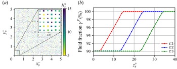


 Open access