


1. Introduction
Screech tones are observed in jets operating away from their design Mach number, appearing as high-amplitude discrete peaks in the acoustic spectrum. Along with broadband shock-associated noise (BBSAN) and turbulent-mixing noise, they form the three components of supersonic jet noise (Tam Reference Tam1995). The appearance of screech tones is undesirable due to both the high intensity noise emitted and the potential to induce vibrations in the surrounding structure, which can lead to failure (Berndt Reference Berndt1984; Raman, Panickar & Chelliah Reference Raman, Panickar and Chelliah2012). These characteristics of screech tones have led to many studies on understanding and mitigating the phenomenon, as shown by reviews from Raman (Reference Raman1999) and Edgington-Mitchell (Reference Edgington-Mitchell2019).
Jets from round convergent nozzles exhibit screech in discrete modal stages that can be classified into the A1 and A2 axisymmetric modes, the C helical mode and the B and D flapping modes (Merle Reference Merle1957; Davies & Oldfield Reference Davies and Oldfield1962; Powell, Umeda & Ishii Reference Powell, Umeda and Ishii1992). Powell (Reference Powell1953a,Reference Powellb) first described screech as arising from a resonance feedback loop within the jet. This loop is comprised of four stages (Edgington-Mitchell Reference Edgington-Mitchell2019). The first is a downstream-propagating disturbance, which travels with the flow until reaching some point downstream. At this downstream point there is a conversion from a downstream-propagating disturbance into an upstream-propagating one. This upstream-propagating disturbance then travels back until reaching an upstream reflection point, where it creates a new downstream-propagating disturbance, completing the resonance loop. The present work here considers free jets and, thus, the upstream and downstream reflection points take the form of the nozzle plane and shock-cell structure, respectively.
A better understanding of screech can only be achieved through knowledge of the underlying physics involved in each step of the resonance cycle. Since the identification of coherent structures in high-speed jets, by Mollo-Christensen (Reference Mollo-Christensen1967) and Crow & Champagne (Reference Crow and Champagne1971), was previously considered to be dominated by stochastic processes, considerable effort has been directed towards the modelling and prediction of these structures. For jet screech, such modelling involves considering the forms that the downstream- and upstream-propagating disturbances take. Initially these were modelled to take the form of a Kelvin–Helmholtz (KH) instability and a free-stream sound wave, respectively (Powell Reference Powell1953b). Recent results have shown that the upstream-travelling mode is a guided jet mode, first studied by Tam & Hu (Reference Tam and Hu1989) and known to exist over a finite frequency range (Towne et al. Reference Towne, Cavalieri, Jordan, Colonius, Schmidt, Jaunet and Brès2017). The work of Shen & Tam (Reference Shen and Tam2002) was the first to consider the upstream-propagating guided jet mode ( $k^{-}_{p}$) as the closure mechanism for the resonance loop in a free jet. They proposed that whilst screech modes A1 and B were still closed by the free-stream acoustic mode, it was the $k^{-}_{p}$ mode that closed resonance for the A2 and C modes. The finite existence region, frequencies over which the mode is propagative for a given set of jet parameters, of the $k_{p}^{-}$ mode was considered by both Gojon, Bogey & Mihaescu (Reference Gojon, Bogey and Mihaescu2018) and Edgington-Mitchell et al. (Reference Edgington-Mitchell, Jaunet, Jordan, Towne, Soria and Honnery2018) for a single jet. In these works the A1 and A2 screech modes were shown to be encompassed by the frequencies defining this existence region, and so could be explained by the characteristics of the $k_{p}^{-}$ mode.
Screech-frequency predictions were then performed using a vortex-sheet model for a single jet by Mancinelli et al. (Reference Mancinelli, Jaunet, Jordan and Towne2019). This followed the resonance criteria set out in Landau & Lifshitz (Reference Landau and Lifshitz2013), later applied to the case of jet-edge interactions by Jordan et al. (Reference Jordan, Jaunet, Towne, Cavalieri, Colonius, Schmidt and Agarwal2018). These predictions were made considering a  $k^{-}_{p}$ mode and showed close agreement with experiments, in contrast with the poor agreement achieved by considering resonance to be closed by free-stream sound waves. Later, Mancinelli et al. (Reference Mancinelli, Jaunet, Jordan and Towne2021) showed that improvements could be made in these screech-frequency predictions by instead considering a finite-thickness model. The presence of the $k^{-}_{p}$ mode in the resonance cycle was also confirmed both experimentally and by linear stability analysis in Edgington-Mitchell et al. (Reference Edgington-Mitchell, Wang, Nogueira, Schmidt, Jaunet, Duke, Jordan and Towne2021). Following the hypothesis of Tam & Tanna (Reference Tam and Tanna1982) they showed that the interaction between the KH mode and the shock-cell structure gives rise to new waves in the flow that may close the resonance loop. Recent work by Edgington-Mitchell et al. (Reference Edgington-Mitchell, Li, Liu, He, Wong, Mackenzie and Nogueira2022) expanded on this and demonstrated that the modal staging behaviour of screech could be explained when considering interactions involving the sub-optimal wavenumbers describing the shock-cell structure. Such sub-optimal wavenumbers arise when taking a Fourier transform of the mean flow in the axial direction and represent the axial variations of the shock-cell structure (Nogueira et al. Reference Nogueira, Jaunet, Mancinelli, Jordan and Edgington-Mitchell2022a). Nogueira et al. (Reference Nogueira, Jordan, Jaunet, Cavalieri, Towne and Edgington-Mitchell2022b) has verified the hypothesis of Tam & Tanna (Reference Tam and Tanna1982), showing how screech is underpinned by an absolute instability mechanism involving the $k_{p}^{-}$ mode and the KH mode, providing a characterisation of the phenomenon in line with early descriptions based on experiments such as Powell (Reference Powell1953b).
Additional complexities arise when considering a twin jet due to acoustic and hydrodynamic interactions between the two jets. This is highlighted in an early study by Seiner, Manning & Ponton (Reference Seiner, Manning and Ponton1988), where pressure amplitudes where found to be more than double the single jet equivalent. Screech tones in a twin-jet system use the same naming convention as for the single jet, with the exception that C is a flapping mode as the system has been shown not to support helical modes (Rodríguez et al. Reference Rodríguez, Stavropoulos, Nogueira, Edgington-Mitchell and Jordan2022). Previous studies (Bell et al. Reference Bell, Soria, Honnery and Edgington-Mitchell2018; Knast et al. Reference Knast, Bell, Wong, Leb, Soria, Honnery and Edgington-Mitchell2018) considered the coupling dynamics at play between the two jets. Bell et al. (Reference Bell, Cluts, Samimy, Soria and Edgington-Mitchell2021) later showing that a round twin-jet system exhibits intermittent coupling and at some jet operating conditions can uncouple entirely. This behaviour was proposed to be due to competition between modes of the flow associated with the different symmetries. The twin-jet vortex sheet was considered previously first by Sedel'Nikov (Reference Sedel'Nikov1967a), Morris (Reference Morris1990) and later Du (Reference Du1993). While in these works the characteristics of both the upstream- and downstream-propagating waves were considered, their roles in resonance were not explored directly. Interest in modelling was renewed by Rodríguez, Jotkar & Gennaro (Reference Rodríguez, Jotkar and Gennaro2018) and Nogueira & Edgington-Mitchell (Reference Nogueira and Edgington-Mitchell2021). The former studied KH instabilities in subsonic twin jets using parabolised stability equations, whilst the latter applied a spatial stability analysis to explore coupling and resonance behaviour of a supersonic twin-jet system with an ideally expanded jet Mach number ( $M_{j}$) of 1.7. This latter study linked the $k^{-}_{p}$ mode to twin-jet resonance at those specific conditions. The analysis was limited to a single set of jet conditions for which experimental data was available. The success of linear stability analysis in predicting the coherent structures and screech characteristics in this previous work suggests such a framework may shed light on the underlying resonance mechanism for other conditions.
In this work, linear stability analysis will be performed for the twin-jet system using both vortex-sheet and finite-thickness models, with comparisons made to experimental acoustic data. The parameter space will be limited to relatively low supersonic Mach numbers where the system exhibits axisymmetric screech modes, as prior modelling efforts for single screeching jets indicate that the vortex-sheet approximation performs best at these conditions (Mancinelli et al. Reference Mancinelli, Jaunet, Jordan and Towne2019, Reference Mancinelli, Jaunet, Jordan and Towne2021).
The paper is organised as follows. The twin-jet set-up and experimental methodology are detailed in § 2. In § 3 the mathematical models for both the vortex-sheet, finite-thickness and screech-frequency prediction models are outlined. Results are shown in § 4, with concluding remarks made in § 5.
2. Set-up
The round twin-jet set-up considered here is as shown in figure 1(a) with  $x$ the axial direction orientated out of the page. Each jet is of diameter $D$ and has an individual coordinate system, $(r_{1},\theta _{1})$ and $(r_{2},\theta _{2})$, in $r$ and $\theta$. The separation of the jets is measured centre-to-centre and denoted by $S$, which is normalised by $D$. In this configuration solutions can be classified based on their symmetries about the $x$–
$x$– $y$ and $x$–
$x$– $z$ planes. These solutions are classified as SS, SA, AS and AA (Rodríguez et al. Reference Rodríguez, Jotkar and Gennaro2018), which is the convention now commonly used in the literature among both round (Nogueira & Edgington-Mitchell Reference Nogueira and Edgington-Mitchell2021; Stavropoulos et al. Reference Stavropoulos, Mancinelli, Jordan, Jaunet, Edgington-Mitchell and Nogueira2022) and rectangular (Yeung, Schmidt & Brès Reference Yeung, Schmidt and Brès2022) twin-jet studies. The first letter (S or A) denotes symmetry or antisymmetry about the $x$–
$x$– $y$ plane and the second about the $x$–
$x$– $z$ plane. These symmetries are visualised in figure 2. In the present work attention is focused solely on the axisymmetric, A1 and A2, screech modes. As such, only twin-jet symmetries that allow axisymmetric solutions will be investigated. This results in only the SS and SA symmetries being considered as AS and AA symmetries cannot support axisymmetric solutions.
(a) Twin-jet set-up and (b) experimental set-up.

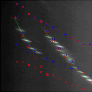
Visualisation of the twin-jet solution symmetries considered in this work, (a) SS and (b) SA. Shown are the real components of the  $k_{p}^{-}$ $(0,2)$ pressure eigenfunctions found using the finite-thickness twin-jet model with $S = 2$, $Mj = 1.16$, $St = 0.69$, $\delta = 0.2$.

Acoustic measurements were taken at the supersonic jet anechoic facility (SJAF) in the Laboratory for Turbulence Research in Aerospace and Combustion (LTRAC) at Monash University. Details on the facility can be found in Wong et al. (Reference Wong, Kirby, Jordan and Edgington-Mitchell2020) with the nozzle plate design described in Knast et al. (Reference Knast, Bell, Wong, Leb, Soria, Honnery and Edgington-Mitchell2018). The twin-jet nozzles have an exit diameter of 8 mm and are purely converging unheated jets. Measurements are taken using a GRAS Type 46BE 1/4 in. pre-amplified free-field microphone with a frequency range of 4 Hz–100 kHz, calibrated using a GRAS 42AB sound calibrator. It is positioned at a distance of  $33D$ downstream and $29D$ in the radial direction, taken from the centre of the system as seen in figure 1(b). For each spacing, the nozzle pressure ratio (NPR) was varied from 2–2.5 in increments of 0.025, with a total of 1M samples obtained at an acquisition frequency of 200 kHz for each NPR. Acoustic power spectral densities (PSD) are obtained through a fast Fourier transform applied using the Welch method (Welch Reference Welch1967) with 75 % overlap for 4096 points to ensure a fine discretisation in frequency.
3. Mathematical models
3.1. Vortex-sheet model
In the vortex-sheet approximation the jet boundary is represented by an infinitesimal shear layer (Lessen, Fox & Zien Reference Lessen, Fox and Zien1965; Sedel'Nikov Reference Sedel'Nikov1967b; Michalke Reference Michalke1970; Morris Reference Morris2010). Within the locally parallel framework, the streamwise velocity is taken as constant within the jet and zero outside of it. Following Morris (Reference Morris1990) and Du (Reference Du1993) the flow is divided into mean and perturbed components. Applying the normal mode ansatz to the perturbed component, the pressure field may be written as
 \begin{equation} \tilde{P}(x,r_{1,2},\theta_{1,2},t)=P(r_{1,2},\theta_{1,2})\, {\rm e}^{{-{\rm i} \omega t + {\rm i} k x}}, \end{equation}
with  $k$ the wavenumber and $\omega$ the angular frequency. Upon substitution into the Euler equations this allows an equation for the perturbed pressure amplitude to be written as
 \begin{equation} \frac{\partial^2 P}{\partial r_{1,2}^2}+\frac{1}{r_{1,2}}\frac{\partial P}{\partial r_{1,2}}+\frac{1}{r_{1,2}^2}\frac{\partial^2 P}{\partial \theta_{1,2}^2}-\lambda^2_{i,o}P = 0, \end{equation}
where subscripts  $i$ and $o$ denote inner, within the jet, and outer, outside of the jet, solutions, respectively, and
 \begin{equation} \left.\begin{gathered} \lambda_{i} = \sqrt{k^2 -\frac{1}{T}(\omega-Mk)^2}, \\ \lambda_{0} = \sqrt{k^2 -\omega^2}. \end{gathered}\right\} \end{equation}
Here  $M$ is the acoustic Mach number and $T$ the temperature ratio between jet and free stream. Quantities are normalised using the free-stream density, free-stream sound speed and jet diameter. Solutions of this equation for both inner and outer regions expressed in forms consistent with the symmetry classification defined above are given by
 \begin{align} P_{i}(r_{1,2},\theta_{1,2})&= \sum_{m=0}^{\infty}\hat{A}_{m}{\rm I}_{m}(\lambda_{i}r_{1,2})\cos(m\theta_{1,2}) + \hat{B}_{m}{\rm I}_{m}(\lambda_{i}r_{1,2})\sin(m\theta_{1,2}), \end{align}
 \begin{align} P_{o}(r_{1},\theta_{1},r_{2},\theta_{2}) &=\sum_{m=0}^{\infty}A_{m}[{\rm K}_{m}(\lambda_{0}r_{1})\cos(m\theta_{1})+({-}1)^m {\rm K}_{m}(\lambda_{0}r_{2})\cos(m\theta_{2})] \nonumber\\ &\quad +\sum_{m=0}^{\infty}B_{m}[{\rm K}_{m}(\lambda_{0}r_{1})\cos(m\theta_{1})-({-}1)^m {\rm K}_{m}(\lambda_{0}r_{2})\cos(m\theta_{2})]\nonumber\\ &\quad +\sum_{m=1}^{\infty}C_{m}[{\rm K}_{m}(\lambda_{0}r_{1})\sin(m\theta_{1})-({-}1)^m {\rm K}_{m}(\lambda_{0}r_{2})\sin(m\theta_{2})]\nonumber\\ &\quad +\sum_{m=1}^{\infty}D_{m}[{\rm K}_{m}(\lambda_{0}r_{1})\sin(m\theta_{1})+({-}1)^m {\rm K}_{m}(\lambda_{0}r_{2})\sin(m\theta_{2})], \end{align}
with  $m$ the azimuthal mode number and $\textrm {I}_{m}$, $\textrm {K}_{m}$ the modified Bessel functions of first and second kind, respectively. Each line of (3.5) corresponds to one of the four solutions, SS, SA, AS, AA mentioned previously. In (3.4) the first term corresponds to SS and SA symmetry, whilst the second to AS and AA symmetry.
To proceed further it is necessary to re-cast the outer solution into a function of only a single coordinate system. This is shown just for the SS symmetry solution and can be achieved through the Bessel addition formula (Lee & Chen Reference Lee and Chen2011), such that
 \begin{equation} {\rm K}_{m}(\lambda_{0}r_{2})\cos(m\theta_2) = \sum_{n={-}\infty}^{\infty}({-}1)^n {\rm K}_{m-n}(\lambda_{0}S) {\rm I}_{n}(\lambda_{0}r_{1})\cos(n\theta_1). \end{equation}
Equation (3.6) can then be substituted into (3.5) which, after simplification, yields
 \begin{align} P_{o}(r_{1},\theta_{1}) &=\sum_{n=0}^{\infty}A_{n}\delta_{mn}{\rm K}_{n}(\lambda_{0}r_{1})\cos(n\theta_{1})\nonumber\\ &\quad +({-}1)^n \epsilon_{n} {\rm I}_{n}(\lambda_{0}r_{1})\cos(n\theta_{1}) \sum_{m=0}^{\infty}A_{m}({-}1)^m [{\rm K}_{m-n}(\lambda_{0}S)+{\rm K}_{m+n}(\lambda_{0}S)], \end{align}
with  $\delta _{mn}$ the Kronecker delta and $\epsilon _{n} = 0.5$ for $n = 0$, and $\epsilon _{n} = 1$ otherwise. Inner and outer solutions are matched at the ideally expanded jet diameter, $D_{j}$, itself normalised by jet diameter and calculated following Tam & Tanna (Reference Tam and Tanna1982) with a design Mach number of 1. Boundary conditions applied are continuity of pressure and displacement (Morris Reference Morris2010). These are given by
 \begin{gather} P_{i}\left(\frac{D_{j}\lambda_{i}}{2}\right) = P_{o}\left(\frac{D_{j}\lambda_{o}}{2}\right), \end{gather}
 \begin{gather}\frac{\partial P_{i}}{\partial r_{1,2}}_{|r_{1,2}=0.5D_{j}} = \frac{1}{T}\frac{(\omega-kM)^2}{\omega^2}\frac{\partial P_{0}}{\partial r_{1,2}}_{|r_{1,2}=0.5D_{j}}. \end{gather}
Equations (3.4), (3.7), (3.8) and (3.9) can now be combined into a single dispersion relation for the twin-jet system as
 \begin{equation} \sum_{m=0}^{\infty}A_{m}[a_{nn}\delta_{mn}\pm ({-}1)^m c_{mn}] = 0, \end{equation}
with
 \begin{equation} a_{nn} = \frac{1}{\left(1-\dfrac{kM}{\omega}\right)^2}-\frac{1}{T} \frac{\lambda_o}{\lambda_i}\frac{{\rm K}_n^{\prime}\left(\dfrac{D_{j}\lambda_0}{2}\right) {\rm I}_n\left(\dfrac{D_{j}\lambda_i}{2}\right)}{{\rm I}_n^{\prime}\left(\dfrac{D_{j}\lambda_i}{2}\right) {\rm K}_n\left(\dfrac{D_{j}\lambda_0}{2}\right)},\\ \end{equation}
 \begin{align} c_{mn}&= ({-}1)^n\epsilon_n[{\rm K}_{m-n}(\lambda_0S)\nonumber\\ &\quad \pm {\rm K}_{m+n}(\lambda_0S)]\left[\frac{{\rm I}_n\left(\dfrac{D_{j}\lambda_0}{2}\right)}{{\rm K}_n \left(\dfrac{D_{j}\lambda_0}{2}\right)}\frac{1}{\left(1-\dfrac{kM}{\omega}\right)^2}- \frac{1}{T}\frac{\lambda_o}{\lambda_i}\frac{{\rm I}_n\left(\dfrac{D_{j}\lambda_i}{2}\right) {\rm I}_n^{\prime}\left(\dfrac{D_{j}\lambda_0}{2}\right)}{{\rm K}_n\left(\dfrac{D_{j}\lambda_o}{2}\right) {\rm I}_n^{\prime}\left(\dfrac{D_{j}\lambda_i}{2}\right)}\right]. \end{align}
 The  $\pm$ in (3.10) and (3.12) are used to define symmetry or antisymmetry about both the $x$–
$x$– $z$ and $x$–
$x$– $y$ planes as detailed in table 1. A key difference between the dispersion relation for the twin jet and the single jet, studied by Lessen et al. (Reference Lessen, Fox and Zien1965), Michalke (Reference Michalke1970) and Towne et al. (Reference Towne, Cavalieri, Jordan, Colonius, Schmidt, Jaunet and Brès2017), is that the former is unable to be solved for only a single azimuthal mode number, $m$. Instead, by truncating (3.10) to a finite value ( $N$) the system is solved for all $m$ up to $N-1$ for both SS and SA modes.
Value of  $\pm$ terms in twin-jet vortex-sheet model for each solution symmetry.

Equation (3.10) is solved with  $N=20$ for all calculations, with convergence checked up to $N=50$. It is worth noting that (3.11) takes the exact same form as the dispersion relation for a single jet as shown by Towne et al. (Reference Towne, Cavalieri, Jordan, Colonius, Schmidt, Jaunet and Brès2017). This allows for recovery of the single-jet solution at large $S$, as (3.12) tends to 0 as $S\rightarrow \infty$. On this basis, classification of twin-jet solutions is defined based on the equivalent single-jet solution they tend to at large spacing. For a given $\omega$, any value of $k$ that satisfies (3.10) is an eigenvalue of the vortex sheet, and (3.4) and (3.5) are used to build the corresponding pressure eigenfunctions.
3.2. Finite-thickness model
The finite-thickness formulation used here was developed initially by Lajús et al. (Reference Lajús, Sinha, Cavalieri, Deschamps and Colonius2019) and later applied to twin-jet systems by Nogueira & Edgington-Mitchell (Reference Nogueira and Edgington-Mitchell2021). All parameters are non-dimensionalised by the free-stream sound speed and density, and jet diameter. The compressible Euler equations in polar coordinates are linearised assuming disturbances of the form
 \begin{equation} \tilde{P}(x,r,\theta,t) = P(r,\theta)\,{\rm e}^{{{\rm i}(kx-\omega t)}}, \end{equation}
with  $k$ and $\omega$ the non-dimensional streamwise wavenumber and frequency, respectively, and $\tilde {P}$ representing the pressure perturbations. With the linearised Euler equations written in polar coordinates, the symmetry of the mean flow imposes a $\theta$ periodicity in the coefficients of the equations, as $\bar {P}(r,\theta )=\bar {P}(r,\theta +n{\rm \pi} )$ with $n$ an integer. Using this periodicity, disturbances may be written with the Floquet ansatz
 \begin{equation} P(r,\theta) = \hat{P}(r,\theta) \mathrm{e}^{\mathrm{i}\mu\theta}, \end{equation}
where  $\mu$ is the Floquet exponent, associated with the different symmetries supported by the flow. Computations then need only be done on a subsection of the azimuthal domain (for this case, in the interval $\theta =[{-{\rm \pi} }/{2},{{\rm \pi} }/{2})$ from figure 1a), reducing the computational cost; disturbances are extended to the entire cross-plane via (3.14). This leads to a generalised eigenvalue problem, expressed here in terms of pressure, of the form
 \begin{equation} \boldsymbol{L}\hat{P} = k\boldsymbol{R}\hat{P}, \end{equation}
with operators  $\boldsymbol {L}$ and $\boldsymbol {R}$ functions of the mean flow, its derivatives and flow variables $\omega$, $M_{j}$, $S$,
$S$,  $\mu$ and the ratio of specific heats $\gamma$. When solving, a Fourier discretisation is used in azimuth and Chebyshev polynomials in radius (Trefethen Reference Trefethen2000), with boundary conditions imposed following Nogueira & Edgington-Mitchell (Reference Nogueira and Edgington-Mitchell2021), and the matrix operators described in Appendix A. The numerical mapping of Bayliss & Turkel (Reference Bayliss and Turkel1992) is applied to ensure appropriate resolution in the shear layer of the jets. Sparsity of the system is also considered, which further reduces the computational cost of the method.
This formulation introduces the need for a velocity profile as an input, which is not required when using the vortex-sheet model. Two hyperbolic tangent velocity profiles, one for each jet, of the same form used in Michalke (Reference Michalke1971),
 \begin{equation} U(r) = M\left[0.5+0.5\tanh\left(\left(\frac{R_{j}}{r}-\frac{r}{R_{j}}\right)\frac{1}{2\delta}\right)\right], \end{equation}
are considered following Nogueira et al. (Reference Nogueira, Jaunet, Mancinelli, Jordan and Edgington-Mitchell2022a) with  $M$ the acoustic Mach number, $R_{j}$ the ideally expanded jet radius and $\delta$ used to characterise the shear-layer thickness. The corresponding twin-jet mean flow is then constructed through the addition of these two single-jet mean flows, following Rodríguez (Reference Rodríguez2021). In each case, the mean temperature is obtained from (3.16) through the Crocco–Busemann relation. An example of a typical mean flow used is provided in figure 3, here visualised over both jets. Equation (3.15) is solved over a domain length of 4 $S$; a domain length of 8 $S$ was found to yield negligible change in the computed wavenumbers.
Sample twin-jet mean flow,  $U$, used for the finite-thickness model for $M_j = 1.16$, $S = 3$, $\delta = 0.2$.

3.3. Prediction model
Screech-frequency predictions are performed using the model developed in Jordan et al. (Reference Jordan, Jaunet, Towne, Cavalieri, Colonius, Schmidt and Agarwal2018) and Mancinelli et al. (Reference Mancinelli, Jaunet, Jordan and Towne2019, Reference Mancinelli, Jaunet, Jordan and Towne2021), applied in these previous works to jet-edge interaction tones and for single-jet screech, respectively. This model considers two reflection points in the flow: the first (upstream) is the nozzle lip, where the KH mode is excited; the second (downstream) is the  $s$th shock cell, where the upstream wave is considered to be generated (Mancinelli et al. Reference Mancinelli, Martini, Jaunet, Jordan, Towne and Gervais2023). It may be used to impose both phase and amplitude criteria (Jordan et al. Reference Jordan, Jaunet, Towne, Cavalieri, Colonius, Schmidt and Agarwal2018; Mancinelli et al. Reference Mancinelli, Jaunet, Jordan and Towne2019, Reference Mancinelli, Jaunet, Jordan and Towne2021). Following the neutral-mode assumption (Mancinelli et al. Reference Mancinelli, Jaunet, Jordan and Towne2021), only the phase criterion is considered here,
 \begin{equation} k^{+}-k_{p}^{-} = \frac{(2p+\phi){\rm \pi}}{L_{s}}, \end{equation}
with  $k^{+}$ the real component of the KH mode wavenumber, $p$ the number of cycles included in the resonance loop, $\phi$ the phase between reflection coefficients as a fraction of ${\rm \pi}$ and $L_{s}$ the distance between the nozzle lip and the $s$th shock cell. This distance is given by
 \begin{equation} \left.\begin{gathered} L_{1} = \frac{\rm \pi}{2.4048}\sqrt{M_{j}^{2}-1},\\ L_{s} = ((1-\alpha)s+\alpha)L_{1}, \end{gathered}\right\}\end{equation}
with  $\alpha = 0.06$ the shock-cell length decrease rate with downstream distance (Harper-Bourne & Fisher Reference Harper-Bourne and Fisher1974) and $L_{1}$ the first shock-cell length from Pack (Reference Pack1950). More recent considerations of (3.18) have also shown the strong alignment with it when compared with experiments (Mancinelli et al. Reference Mancinelli, Jaunet, Jordan and Towne2021). The distances to each shock cell could also be computed via simulation, such as a Reynolds-averaged Navier–Stokes simulation (RANS); however, for the purpose of this work in drawing comparisons between the feedback loops in single and twin jets, the simple model of (3.18) is sufficient. For any pair of wavenumbers ( $k^{+}$, $k_{p}^{-}$), obtained by solving (3.10) or (3.15), that satisfy (3.17) for given $s$,
$s$,  $p$ and $\phi$, the corresponding frequency is then a prediction of the screech frequency. As shown in Mancinelli et al. (Reference Mancinelli, Jaunet, Jordan and Towne2021), this resonance model can lead to similar frequency predictions compared with the absolute instability framework for the right choice of parameters. Note, however, that the specific values of $p$ and $s$ used for a given prediction are less important than the ratio of the two, $p/s$. For the specific case of $\phi = 0$, this ratio is equivalent to the ratio between the standing-wave wavenumber ( $k_{sw}$) and the shock-cell wavenumber ( $k_s$) (Mancinelli et al. Reference Mancinelli, Jaunet, Jordan and Towne2021). As mentioned previously, multiple wavenumbers, dominant ( $k_{s1}$) and sub-optimal ( $k_{s2}$), are required to accurately describe the shock-cell variation (Nogueira et al. Reference Nogueira, Jaunet, Mancinelli, Jordan and Edgington-Mitchell2022a). Equation (3.17) does not consider sub-optimal wavenumbers and, thus, agreement between it and the wave interaction model outlined by Tam & Tanna (Reference Tam and Tanna1982) occurs only when considering $k_{s1}$. Such agreement occurs for a value of $p/s = 1$ (Mancinelli et al. Reference Mancinelli, Jaunet, Jordan and Towne2021). This indicates that any prediction using (3.17) with $p/s = 1$ corresponds to a consideration of the dominant wavenumber and anywhere $p/s\neq 1$ corresponds to the wavenumbers describing the axial variation in the shock-cell spacing.
4. Results
4.1. Comparison to past formulations
To validate the numerical implementation of (3.10), a comparison is performed with Morris (Reference Morris1990) and Du (Reference Du1993) who had both previously calculated dispersion relation eigenvalues of the twin-jet vortex-sheet model. These calculations were made for  $M_{j} = 1.32$, $St = 1/{\rm \pi}$ and a jet temperature ratio based on an isentropic expansion, where $St$ is the non-dimensional frequency defined by $St = f\kern0.7pt D/U_j$. Only the symmetries SS and SA are considered for $m = 0,1,2$. The nomenclature for solution symmetry used in these previous works differs from the current convention with a guide between them provided in table 2, note that Du (Reference Du1993) had mislabelled family 3 and 4 solutions that has been rectified in the present table. Figure 4(a) shows the results of Morris (Reference Morris1990) with those from (3.10) overlaid for SS symmetry. Plotted are the growth rates of the KH mode for the first three azimuthal modes. It can be seen that the results obtained here match the previous work. Conversely, in figure 4(b) the growth rates for SA do not match. A comparison between the current work and Du (Reference Du1993) for both SS and SA growth rates is shown in figure 5, they can be seen to be in agreement; Du (Reference Du1993) also noted a mismatch with the results of Morris (Reference Morris1990). Note that the formulation used here and in Du (Reference Du1993) is identical to that provided in Morris (Reference Morris1990), suggesting that the discrepancy may arise due to an implementation error in the earlier work rather than a theoretical one. With the current twin-jet vortex-sheet model validated, it can be used with confidence for the remainder of this study. Details about the finite-thickness formulation can be found in Nogueira & Edgington-Mitchell (Reference Nogueira and Edgington-Mitchell2021).
Symmetry notation for solutions of a twin-jet vortex sheet.

Comparison between the computed KH growth rates with those of Morris (Reference Morris1990) for (a) SS and(b) SA with  $M_j = 1.32$ and $St = 1/{\rm \pi}$. Note that growth rate values plotted here are scaled by jet radius.

Comparison between the computed KH growth rates with those of Du (Reference Du1993) for (a) SS and (b) SA with  $M_j = 1.32$ and $St = 1/{\rm \pi}$. Note that growth rate values plotted here are scaled by jet radius.

4.2. Waves involved in screech
4.2.1. Characteristics of KH and  $k_{p}^{-}$ modes

Before considering resonance, an overview of the behaviour of both the KH and  $k_{p}^{-}$ modes in a twin-jet system is considered. Eigenvalues of the dispersion relation calculated using (3.10) are plotted in figure 6, as in Tam & Hu (Reference Tam and Hu1989). Here results are presented for an isentropic temperature ratio, $M_{j} = 1.16$ and $S = 2$ and 50. In figure 6(a) classification in the form $(m,n_{r})$ of the relevant modes is highlighted, where $m$ is the azimuthal mode number and $n_{r}$ the radial mode number. The latter corresponds to the number of anti-nodes present in the pressure eigenfunction, as shown by (Tam & Hu Reference Tam and Hu1989; Towne et al. Reference Towne, Cavalieri, Jordan, Colonius, Schmidt, Jaunet and Brès2017; Edgington-Mitchell et al. Reference Edgington-Mitchell, Jaunet, Jordan, Towne, Soria and Honnery2018; Gojon et al. Reference Gojon, Bogey and Mihaescu2018). Since the modes plotted here are neutrally convectively stable with negative phase speed, the sign of the slope indicates their propagation direction (group velocity): downstream-propagating waves, denoted $k^{+}_{d}$, have a positive slope, and $k^{-}_{p}$ have a negative slope. Similar to the single-jet case (Tam & Hu Reference Tam and Hu1989), it is observed that the $k^{-}_{p}$ modes exist over a finite range of frequencies. The smallest frequency at which it exists is known as the branch point, and the highest frequency is characterised by a saddle point between $k^{+}_{d}$ and $k^{-}_{p}$ (Towne et al. Reference Towne, Cavalieri, Jordan, Colonius, Schmidt, Jaunet and Brès2017). Comparing the results between figures 6(a) and 6(c), $S = 2$, with figures 6(b) and 6(d), $S = 50$, the existence region of the $k^{-}_{p}$ ( $0,2$) mode is strongly affected by the jet spacing only for SA. The branch points for SA are seen to decrease in value significantly as $S$ increases, resulting in an increase in the $k_{p}^{-}$ ( $0,2$) existence region for increasing $S$. This trend suggests that coupling between the two jets may act to hinder the propagation of the SA symmetry $k_{p}^{-}$ mode. The changes observed for SS symmetry are significantly smaller, with a slight increase in the ( $1,1$) branch point and a slight (<1 %) decrease in the ( $0,2$) branch point. The existence region of the SA symmetry $k_{p}^{-}$ is smaller than that of SS symmetry throughout figure 6. The dispersion relation plots for SS and SA display non-negligible differences between the two symmetries even at $S = 15$; this suggests that resonant modes may be coupled for high inter-jet distances, which has also been observed experimentally (Shaw Reference Shaw1990; Knast et al. Reference Knast, Bell, Wong, Leb, Soria, Honnery and Edgington-Mitchell2018). The value of $S$ chosen for figures 6(b) and 6(d) is such that it represents a jet separation where the twin-jet system can be considered to behave as a single-jet system. There does not currently exist a unique metric for determining at which $S$ this occurs. For this work, we focus on the axisymmetric screech modes, for which the $k_{p}^{-}$ ( $0,2$) mode and its frequency band of existence is of importance. As such, the metric considered will be the frequency discrepancy, in $St$, between the SA $k^{-}_{p}$ ( $0,2$) branch point and that of the single jet. Figure 7(a) shows the change in SA branch point at $M_j = 1.16$ across $S$, where it can be seen to exhibit an asymptotic convergence towards the single-jet value. Highlighting that whilst it is at low $S$ where the effect of the second jet is most relevant, there is still a non-negligible effect from the second jet even at greater $S$. Note that at higher $S$ the difference in $St$ becomes lower than the resolution used ( $\Delta St = 0.0005$) resulting in the curve no longer appearing smooth. The fractional difference between the single- and twin-jet values is given across $S$ in figure 7(b). Given the asymptotic behaviour, the condition for the twin-jet system behaving as single jets is defined as when this difference is equal to 0.01 (1 % difference between twin-jet and single-jet values). From figure 7(b) this would correspond to an $S$ of 50. Hence, the use of $S = 50$ in figure 6 for comparison with the low spacing ( $S = 2$) case. It is, however, important to recognise that the value of $S = 50$ holds only for considerations of the $k_{p}^{-}$ ( $0,2$) branch point, for example, if instead the wavenumber or growth rates of the KH mode were considered then this would result in a much smaller value of $S$ as these values converge more quickly to the single-jet value (Morris Reference Morris1990; Rodríguez et al. Reference Rodríguez, Stavropoulos, Nogueira, Edgington-Mitchell and Jordan2022).
Dispersion relation eigenvalues for  $M_{j} = 1.16$ for (a) SS, $S = 2$; (b) SS, $S = 50$; (c) SA, $S = 2$; and (d) SA, $S = 50$, plotted here are just modes corresponding to $m = 0$ and 1. Branch (blue) and saddle (green) points are highlighted. Also shown is the sonic line (yellow) for sound waves travelling upstream. Note that the green and blue bounds for the $(1,1)$ mode appear to be almost superimposed due to the close proximity of the branch and saddle points.

Comparison of SA  $k_{p}^{-}$ ( $0,2$) branch point with the single-jet value for the $M_j = 1.16$ jet. This is compared directly in (a) and as a fraction in (b), also marked on (b) in red is the line corresponding to a 1 % divergence from the single-jet value.

The amplitude structure of the  $k_p^{-}$ ( $0,2$) and KH mode eigenfunctions can be obtained from the vortex-sheet model using (3.4) and (3.5). This allows for differences in structure between SS and SA type solutions to be visualised. In figure 8(a) the eigenfunction structure for the KH mode are compared for SS and SA plotted along the $y$ axis of figure 1. A key difference occurs in the region between the two jets: due to the symmetry of the problem, the SA solution is forced to reach zero pressure at the centre point, whereas the SS solution is forced to reach a zero pressure gradient. Outside of this region the two profiles are seen to be identical. Conversely, in figure 8(b) the eigenfunction structures of the $k^{-}_{p}$ ( $0,2$) modes exhibit significant differences between the SS and SA symmetries. Between the two jets the SS solution has higher amplitude than the SA, whilst the opposite occurs away from each jet where the SA solution has a higher amplitude than the SS. The general behaviour of both the KH and $k_{p}^{-}$ modes outside the inter-jet region, as would be expected, follows the single-jet case (Tam & Hu Reference Tam and Hu1989). The KH mode peaks along the jet boundary and decays away radially, whilst the $k^{-}_{p}$ mode peaks at the centreline before decaying away more slowly. Differences between single- and twin-jet eigenfunctions arise from the aforementioned behaviour in the inter-jet region.
Absolute value of normalised pressure eigenfunctions along the  $y$ axis for SS (red) and SA (black), (a) KH ( $m = 0$) and (b) $k^{-}_{p}$ ( $0,2$) mode. Here $M_j = 1.16$, $S = 3$ and $St = 0.67$. Jet edges are highlighted in blue.

Eigenfunctions for the KH and  $k_{p}^{-}$ ( $0,2$) modes can also be found using the finite-thickness model, which allows for insight into how the velocity profile affects the pressure eigenfunctions. These are plotted in figures 9 and 10 for the same jet parameters as in figure 8 with values of $\delta$ as 0.12, 0.2 and 0.4. There are two main behaviours that can be seen in figure 9. Within the jet itself, all the models agree well with each other and there is essentially no difference between them. This changes outside the jet core. For SS, figure 9(a), increasing shear-layer thickness causes a more rapid radial decay in both the inter-jet and outer regions. This trend is also observed for SA, figure 9(b). When considering the region between the jets, the SA eigenfunctions all converge to zero at the midpoint to satisfy the symmetry condition, with the change in $\delta$ seen to have only a small effect on the curvature here. There is less agreement observed between the vortex-sheet and finite-thickness model for the KH mode, as shown in figure 10. As was seen for the $k_{p}^{-}$ ( $0,2$) mode, the KH modes predicted using the finite-thickness model decrease in magnitude outside the jet more quickly than in the vortex-sheet model. Inside the jet, the KH modes all follow the same shape but lie apart from each other, with very little overlap of profiles. There is a dissymmetry seen in the amplitude peaks of the KH eigenfunction when considering the finite-thickness model, that is not seen for the vortex-sheet model. As the shear-layer thickness increases, the amplitude of the eigenfunction at the outer mixing layer is seen to decrease slightly.
Absolute value of normalised  $k_p^{-}$ ( $0,2$) pressure eigenfunctions along the $y$ axis for both the vortex-sheet model and varying velocity profiles in the finite-thickness model. Here $M_j = 1.16$, $S = 3$ and $St = 0.67$. Only one jet is shown for both the inter-jet ( $y/D <1$), inner ( $1< y/D<2$) and outer ( $y/D >2$) regions. Results are shown for (a) SS and (b) SA. Vortex sheet (black), $\delta = 0.12$ (blue), $\delta = 0.2$ (red) and $\delta = 0.4$ (green).

Absolute value of normalised KH ( $m = 0$) pressure eigenfunctions along the $y$ axis for both the vortex-sheet model and varying velocity profiles in the finite-thickness model. Here $M_j = 1.16$, $S = 3$ and $St = 0.67$. Only one jet is shown for both the inter-jet ( $y/D <1$), inner ( $1< y/D<2$) and outer ( $y/D >2$) regions. Results are shown for (a) SS and (b) SA. Vortex sheet (black), $\delta = 0.12$ (blue) and $\delta = 0.2$ (red). For $\delta = 0.4$, the KH mode has stabilised.

4.2.2. Branch and saddle point bounds
As was shown in § 4.2.1, and noted in Du (Reference Du1993), the existence region of the  $k_{p}^{-}$ mode is dependent on jet spacing in twin jets. Here this dependence is considered more closely across multiple $S$ and $M_j$ for the $k_{p}^{-}$ ( $0,2$) mode. This existence region is important when considering the $k_p^{-}$ mode to close the screech feedback loop, as it then serves as a bound for where screech modes may occur. Any variation in the frequency range over which the $k_p^{-}$ modes are propogative can be associated with variations in the frequency range over which screech tones are to be expected. In figure 11 the effect of $M_j$, $S$ and symmetry on the branch and saddle points are shown for $S = 2$, 3, 4, 6 using the vortex-sheet model. Only $M_j$ up to 1.16 are considered due to the focus of this paper on axisymmetric screech modes. As $M_j$ increases, both the branch and saddle points decrease smoothly, following the same trend as the single-jet case (Mancinelli et al. Reference Mancinelli, Jaunet, Jordan and Towne2019). For the SS symmetry, it is seen in figure 11(a) that changing $S$ influences neither the branch-point nor the saddle-point values. In contrast, the SA symmetry (figure 11b) is observed to be heavily dependent on $S$. As the jet spacing increases, the SA branch-point frequency decreases, resulting in an increase in the existence region of the $k_p^{-}$ ( $0,2$) mode. The saddle points of the SA modes remain unchanged with $S$.
$S$.
Variation in branch (blue) and saddle (green) points with  $M_j$ and $S$ for the $k_p^{-}$ ( $0,2$) mode using the vortex-sheet model. Computed for SS (a) and SA (b) with $+$
$+$  $S = 2$, $\times$ $S = 3$, $\circ$ $S = 4$ and $\square$ $S = 6$.

Variation of branch and saddle points with shear-layer thickness is considered in figure 12, this is achieved through varying the parameter  $\delta$ of (3.16) in the range 0.12, 0.2 and 0.4. These values were calculated using a $\Delta St$ of 0.01, which may lead to some uncertainty in the values obtained, causing the slight oscillations observed in figure 12. Both the SS, figure 12(a), and the SA symmetry, figure 12(b), have an existence region that varies with $\delta$. This is in line with the single-jet case, which also exhibited this behaviour (Mancinelli et al. Reference Mancinelli, Jaunet, Jordan and Towne2021). Across all values of $\delta$ the existence region of SS is greater than SA. In figure 12 the saddle points also have a dependence on $\delta$ and decrease slightly as it increases. When using the finite-thickness model, figure 12, the existence region of SA symmetry is noticeably greater than that found with the vortex-sheet model, figure 11. Thus, when considering a screech feedback loop closed by the $k_p^{-}$ ( $0,2$) mode, the finite-thickness model predicts a larger range over which SA symmetry screech tones may be supported.
Variation in branch (blue) and saddle (green) points with  $M_j$ and $\delta$ for the $k_p^{-}$ ( $0,2$) mode using the finite-thickness model. Computed for (a) SS and (b) SA. Here $S = 3$ with $+$
$+$  $\delta = 0.12$, $\times$ $\delta = 0.2$ and $\circ$ $\delta = 0.4$.

4.3. Predictions of screech frequency
4.3.1. Single jet
Screech-frequency predictions are first preformed for the single-jet system. Such an analysis has been done previously using both a vortex-sheet and finite-thickness model (Mancinelli et al. Reference Mancinelli, Jaunet, Jordan and Towne2021). The equivalent predictions are performed using the experimental set-up considered here for both models. Formulation for the single-jet vortex-sheet model is given by (3.11), whilst the finite-thickness formulation follows § 3.2 without the domain extension, and does not require a discretisation in  $\theta$. Predictions are performed using (3.17) over a parameter range of $s = 2- 6$, $p = 2- 6$ and $\phi = 0$, $\frac {1}{4}$, $\frac {1}{2}$, 1. Acoustics for the single jet are presented in figure 13 with predictions from the vortex-sheet model overlaid along with the branch and saddle points of the $k_p^{-}$ ( $0,2$) mode. Best agreement was observed for parameters $s = 4$, $\phi = 0$ and $p = 3$ for the A1 mode, and $s = 4$, $\phi = 0$ and $p = 4$ for the A2 mode. These values are summarised in table 3. Agreement between the model and experimental data is good; however, for each of the A1 and A2 screech modes, there is an over-prediction of the frequency at lower $M_j$ and an under-prediction at higher $M_j$. The branch points of the $k_p^{-}$ ( $0,2$) modes sit just above the end of each tone and so do not coincide precisely with the cutoff of the screech tones. Compared with the previous work of Mancinelli et al. (Reference Mancinelli, Jaunet, Jordan and Towne2021), the key difference is the value of the phase difference between reflection coefficients, $\phi$, used for the screech-frequency predictions. They had found best agreement using $\phi = 1/4$ whereas here that agreement is found for $\phi = 0$, the reflection coefficients being in-phase. This discrepancy would be due to differences in the two facilities, as the screech feedback loop has been noted to display facility sensitivity (Edgington-Mitchell Reference Edgington-Mitchell2019). In this case, an example being the lip thickness of the nozzle that is $15\,\%$ in the current work and $3\,\%$ previously (Mancinelli et al. Reference Mancinelli, Jaunet, Jordan and Towne2021).
Sound pressure levels (dB/St) measured for the single-jet system running at several  $M_j$. Screech-frequency predictions using the vortex-sheet model are shown, along with $k_{p}^{-}$ ( $0,2$) branch and saddle points. Lines highlighting the screech peaks are included. Parameters used for these predictions are $s = 4$, $p = 3$ (A1 mode), 4 (A2 mode) and $\phi = 0$.

Parameters used for single-jet vortex-sheet model predictions.

The equivalent predictions of screech frequency for a single jet using the finite-thickness model are overlaid on the experimental data in figure 14, also shown are the branch and saddle points of the  $k_p^{-}$ ( $0,2$) mode. The hyperbolic tangent profile of (3.16) is used with a value of $\delta = 0.2$ for the velocity profile. This value is chosen to match the value that will be used for twin-jet calculations, and a justification is provided in Appendices B and C. As before, the parameter range of $s = 2- 6$, $p = 2- 6$ and $\phi = 0$, $\frac {1}{4}$, $\frac {1}{2}$, 1 is considered. Best agreement is observed for $s = 4$, $\phi = 0$ and $p = 4$ for the A1 mode, and $s = 4$, $\phi = 0$ and $p = 5$ for the A2 mode, and these parameters are summarised in table 4. Compared with the previous results from the vortex sheet, figure 13, the predictions here align more closely with the experimental screech tones and match them in slope. Thus utilising a model with a more realistic velocity profile is seen to result in better agreement with the experimental data. This agrees with the previous study of Mancinelli et al. (Reference Mancinelli, Jaunet, Jordan and Towne2021) who observed best agreement between model and data for identical velocity profile and parameters as given in table 4. Comparing tables 3 and 4 highlights that the values of $p/s$ are $\neq 1$ (A1) and $=1$ (A2) for the vortex-sheet model, whilst $=1$ (A1) and $\neq 1$ (A2) for the finite-thickness model. This further indicates an improvement when moving to the finite-thickness model as these $p/s$ ratios align with results from Nogueira et al. (Reference Nogueira, Jaunet, Mancinelli, Jordan and Edgington-Mitchell2022a).
Sound pressure levels (dB/St) measured for the single-jet system running at several  $M_j$. Screech-frequency predictions using the finite-thickness model with $\delta = 0.2$ are shown, along with $k_{p}^{-}$ ( $0,2$) branch and saddle points. Lines highlighting the screech peaks are included. Parameters used for these predictions are $s = 4$, $p = 4$ (A1 mode), 5 (A2 mode) and $\phi = 0$.

Parameters used for single-jet finite-thickness model predictions.

4.3.2. Twin jet
Predictions made using a vortex-sheet model can achieve strong qualitative agreement with experiments, as seen previously for the single jet in § 4.3.1. Given the success of such a simple model in the prediction of single-jet screech, its performance is now considered for the twin-jet problem. In figure 15 predictions using the twin-jet vortex-sheet model are plotted over experimental acoustic data using (3.10) and (3.17). A parameter range of  $s = 2- 6$, $p = 2- 6$ and $\phi = 0$, $\frac {1}{4}$, $\frac {1}{2}$, 1 was considered with best agreement found between the model and experimental data for $s = 5$, $\phi = 0$ and $p = 4$ for A1 equivalent screech modes and $s = 5$, $\phi = 0$ and $p = 5$ for A2 equivalent screech modes.These parameters are summarised in table 5. The branch and saddle points for the $k_{p}^{-}$ ( $0,2$) mode are also shown in figure 15. The predictions for SS symmetry are qualitatively close to the experimental peaks. However, in a more quantitative evaluation, the model suffers from under-prediction at higher $M_j$ and over-prediction at lower $M_j$ for both the A1 and A2 branches. This results in the difference in screech tone variation with $M_j$ between predictions and data in figure 15. These results are comparable to those of the single jet, figure 13 and Mancinelli et al. (Reference Mancinelli, Jaunet, Jordan and Towne2021), which displayed the same level of agreement between model and experiment. A key difference between the single- and twin-jet predictions are the parameters used, given in tables 3 and 5. When moving from the single jet to the twin jet, best agreement is found at greater values of $s$ and $p$, suggesting that the downstream reflection point of resonance increases for a twin jet. There is a sharp bounding of both the A1 and A2 axisymmetric screech modes by the SS $k_{p}^{-}$ ( $0,2$) branch points in figure 15, and these screech modes lie entirely within the propagative range of the SS $k_{p}^{-}$ ( $0,2$). This is in contrast to the single-jet vortex-sheet model where the branch points were unable to bound the screech tones, highlighting the improvements found when moving to a twin-jet model. When considering the SA $k_p^{-}$ ( $0,2$) propagative region, the screech modes are observed to lie predominantly outside of it. At $S = 2$, figure 15(a), there is no overlap, whereas a slight overlap is seen for $S$ = 3, figure 15(b), which increases with increasing $S$ in figures 15(c) and 15(d). Thus, the vortex-sheet model suggests that the axisymmetric screech modes observed in a twin-jet system are predominantly SS symmetry for low spacings, and that there are only small regions where SA symmetry could be supported. In the regions where both SS and SA symmetry are permitted the model produces identical predictions for both symmetries, providing no clear way to determine which symmetry the screech mode is expected to be.
Sound pressure levels (dB/St) measured for the twin-jet system running at several  $M_j$ and spacings (a) $S = 2$, (b) $3$, (c) $4$ and (d) $6$. Screech-frequency predictions using the vortex-sheet model are shown for both SS ( $\circ$, red) and SA ( $\square$, blue) symmetries. Along with $k_{p}^{-}$ ( $0,2$) branch and saddle points for SS ( $\times$, red) and SA ( $+$, blue). Lines highlighting the screech peaks are included. Parameters used for these predictions are $s = 5$, $p=4$ (A1 mode), 5 (A2 mode) and $\phi = 0$.

Parameters used for twin-jet vortex-sheet model predictions.

Predictions of the screech frequency for the finite-thickness model are obtained using (3.17) with the  $k_{p}^{-}$ ( $0,2$) and KH wavenumbers computed from (3.15). The value of $\delta$ used in (3.16) is 0.2, which is justified through fitting velocity profiles to experimental particle image velocimetry (PIV) data and considering the region in which the KH mode is unstable (see Appendix B). The same parameter range of $s = 2- 6$, $p = 2- 6$ and $\phi = 0$, $\frac {1}{4}$, $\frac {1}{2}$, 1 was considered; with best agreement found for $s = 4$, $\phi = 0$ and $p = 4$ for the A1 equivalent screech modes, and $s = 4$, $\phi = 0$ and $p = 5$ for the A2 equivalent screech modes, summarised in table 6. These screech-frequency predictions, along with the branch and saddle points of the $k_{p}^{-}$ ( $0,2$) mode, are plotted over the experimental data in figure 16. The parameters used here for best agreement match those found for the single-jet finite-thickness model, table 4. This results in the same $p/s$ ratios ( $=1$ or $\neq 1$) as were seen for the single jet, suggesting that the shock-cell wavenumber (dominant or sub-optimal) associated with each of the A1 or A2 screech modes is the same for the twin-jet system as it is for the single jet. Considering first the branch and saddle points of the $k_{p}^{-}$ ( $0,2$) mode, the screech modes lie entirely within the SS propagative region but there is a less-sharp bounding by the branch and saddle points for this value of $\delta$. The SA propagative region is larger for the finite-thickness model than the vortex-sheet model for all $S$ and, by $S = 6$ (figure 16d), the screech tones are completely bounded by it. Although there is not a sharp lower bound on the screech tones by the SS branch points, as was observed using the vortex-sheet model in figure 15, the saddle points lie significantly closer to the screech tones. Overall this serves as a closer bounding of the screech tones by the SS branch and saddle points, highlighting an immediate improvement in moving from the vortex-sheet model to the finite-thickness model for twin jets. In addition, changing the parameter $\delta$ (or equivalently, choosing a position further upstream/downstream for the analysis) may lead to branch points closer to the lower bounds of the screech tones observed experimentally (Mancinelli et al. Reference Mancinelli, Jaunet, Jordan and Towne2021; Nogueira & Edgington-Mitchell Reference Nogueira and Edgington-Mitchell2021). Predictions obtained with the finite-thickness model offer a clear improvement over those found with the vortex-sheet model, with the slope of the prediction curve aligning closely with the screech tones themselves. This improvement when moving from a vortex-sheet to finite-thickness model matches what was observed for the single jet in § 4.3.1. In regions where the twin-jet finite-thickness model predicts both SS and SA symmetry there are only slight differences seen between the predictions. While this differs from the vortex-sheet model that saw identical predictions, it is still not enough to give any indication of a preferential screech symmetry.
Sound pressure levels (dB/St) measured for the twin-jet system running at several  $M_j$ and spacings (a) $S = 2$, (b) $3$, (c) $4$ and (d) $6$. Screech-frequency predictions using the finite-thickness model are shown for both SS ( $\circ$, red) and SA ( $\square$, blue) symmetries. Along with $k_{p}^{-}$ ( $0,2$) branch and saddle points for SS ( $\times$, red) and SA ( $+$, blue). Lines highlighting the screech peaks are included. Parameters used for these predictions are $s = 4$, $p = 4$ (A1 mode), 5 (A2 mode) and $\phi = 0$.

Parameters used for twin-jet finite-thickness model predictions.

4.3.3. Discussion
In figure 17(a) the screech frequencies of the A1 and A2 axisymmetric screech modes, obtained experimentally, are compared across multiple jet separations and with the single jet. It can be seen that there is near negligible change in screech frequency for the A1 mode, whilst the A2 mode exhibits some slight differences but is also mostly unchanged with spacing. This suggests, primarily for the A1 mode, that the screech frequency is not affected by the jet separation. Figures 17(b) and 17(c) compare the finite-thickness model screech-frequency predictions for both SS and SA symmetry. For SS symmetry, it is seen that the prediction lines lie together with no difference for  $S$, aside from the single-jet prediction that sits just above the others. The SA symmetry, however, exhibits small differences in the prediction lines with spacing and these differences display a noticeable trend with the screech-frequency prediction decreasing with increasing $S$. From this it could be suggested that the A1 screech mode is of SS symmetry, as both the experiment and model predictions are unchanged with $S$. These results do not provide any suggestion for the symmetry of the A2 mode.


The branch points of the  $k_{p}^{-}$ ( $0,2$) SA modes are seen to be sensitive to two main geometric characteristics of the system: $S$ and the shear-layer thickness. From figure 12 these branch points, for the twin-jet finite-thickness model, decrease in frequency as the shear-layer thickness of the mean flow is increased. This then influences where the model predicts SA symmetry modes to occur, as by considering axial locations further downstream when constructing the mean flow it increases the range of frequencies over which the SA $k_{p}^{-}$ mode exists. As such, it could be possible to observe a screech tone of SA symmetry outside of the region predicted by the finite-thickness model in figure 16. This would then indicate that the $k_{p}^{-}$ mode is generated at a distance further downstream than was considered by the mean flow utilised here. The dependence on $S$ by the SA branch points was observed using both twin-jet vortex-sheet and finite-thickness models in figures 11 and 12. It is not currently clear why the SA modes in particular are affected so strongly. The trend, decreasing branch point frequency with increasing $S$, suggests that for lower jet separations, where the jets may be assumed more strongly coupled, this coupling interferes with the propagation of the SA $k_{p}^{-}$ ( $0,2$) mode in some way. Further work to determine the precise nature of this interaction is required and should shed light more generally on the behaviour of the $k_{p}^{-}$ mode.
When considering the vortex-sheet model screech-frequency predictions for both a single jet, § 4.3.1, and twin jet, § 4.3.2, it becomes clear that a single-jet model could not be applied in an attempt to understand twin-jet screech tones. A primary difference for this is the performance of the two models. The twin-jet model is able to bound the screech modes with the branch points of the SS  $k_{p}^{-}$ ( $0,2$) mode (figure 15), whereas such agreement cannot be seen for the single jet where the branch points lie just above the lowest frequencies of the screech modes (figure 13). Additionally, a single-jet model, by construction, cannot provide any information about symmetry. This would leave an important aspect of the twin-jet system unable to be considered. By moving to the twin-jet vortex-sheet model it provides an indication of where each symmetry, SS or SA, could be expected to occur for the screech modes.
Vortex-sheet models utilise an idealised ‘top-hat’ velocity profile that is most accurate very close to the nozzle. For considerations of phenomena that occur at axial locations further downstream, using a finite-thickness model allows for a more realistic velocity profile to be used. Increasing the complexity of the model, by moving to a twin-jet finite-thickness model, results in better agreement with data (figure 16) and allows for the effect of the mean flow to be considered. The region in which SA symmetry screech modes could be expected to occur also increases when moving to the twin-jet finite-thickness model.
The present results indicated the potential for both SS and SA symmetries to be observed experimentally for the A1 and A2 screech modes. In regions where both symmetries are supported, either by the vortex-sheet or finite-thickness twin-jet model, neither model provides enough information to clearly determine a preferred symmetry. The twin-jet finite-thickness model does propose slight differences between SS and SA screech frequencies, with the SA symmetry always occurring at the higher frequency (figure 16), whereas screech frequencies from the twin-jet vortex-sheet model are near identical for the two symmetries (figure 15). The difficulty in discerning symmetry may be due to a competition between screech tones of opposing symmetry. The dominant resonance loop will then be determined by the gain of the resonance loop associated with either SS or SA symmetry. Such a competition between modes was previously put forth by Bell et al. (Reference Bell, Cluts, Samimy, Soria and Edgington-Mitchell2021) as a possible explanation for the intermittent coupling they observed for round twin jets at higher  $Mj$. For the lower $M_j$ considered here, similar intermittency between symmetry may also be occurring, with the current models only able to indicate the competing symmetries. An alternative method could be required, such as the complex-valued model of Mancinelli et al. (Reference Mancinelli, Jaunet, Jordan and Towne2021) or the spatially periodic analysis of Nogueira et al. (Reference Nogueira, Jordan, Jaunet, Cavalieri, Towne and Edgington-Mitchell2022b), to determine the dominant symmetry in such regions where both SS and SA are supported.
Finally, both twin-jet models, vortex sheet and finite thickness, assume that the twin-jet system is coupled. Due to this the models cannot provide any insight into potential uncoupling of the jets, a behaviour that has been observed to occur at higher  $M_j$ (Bell et al. Reference Bell, Cluts, Samimy, Soria and Edgington-Mitchell2021).
5. Conclusions
This investigation used both a vortex-sheet and finite-thickness model to analyse resonance in an under-expanded supersonic twin-jet system running at low supersonic Mach numbers, where the flow is expected to be dominated by axisymmetric disturbances in each jet. Characteristics of both the KH and  $k^{-}_{p}$ ( $0,2$) modes were studied using the models, allowing identification of the frequency range over which resonance may occur. The range over which the $k^{-}_{p}$ ( $0,2$) mode is propagative differs depending on the jet symmetry, SS or SA, the jet spacing, $S$, and the velocity profile used when considering the finite-thickness model. These propagative regions in the vortex-sheet model, for SS and SA, bound the experimental screech tones well, in particular the SS branch points that provide a sharp lower bound for the A1 and A2 modes. For each $S$, the vortex-sheet model generally over-predicts the screech frequency for low $M_j$ and under-predicts them for high $M_j$, but still provides qualitative agreement to the data. Better agreement was seen for the finite-thickness model with predictions closely aligning with the experimental data, resulting in stronger agreement than the vortex-sheet model. Neither model was able to distinguish between predictions of SS and SA symmetry for the screech tones, with only slight differences observed for the finite-thickness model, indicating a potential limitation. It is worth recalling that the screech-frequency predictions made in § 4.3 use linear locally parallel models, and the agreement observed between them and the experimental data is very favourable. The improvement seen in moving from a vortex-sheet to finite-thickness model, along with the prediction parameters used for best agreement, follows what was seen for the single-jet case. This similarity with the single-jet case, along with the strong agreement between the twin-jet models and data, suggests that the feedback loop operating in single and twin jets share similarities and the resonance feedback loop for axisymmetric screech tones in round twin-jets is closed through the twin-jet $k_p^{-}$ ( $0,2$) mode.
Funding
This work was supported by the Australian Research Council under the Discovery Project Scheme: DP190102220. M.N.S. is supported through an Australian Government Research Training Program Scholarship. Computational facilities supporting this project include the Multi-modal Australian ScienceS Imaging and Visualisation Environment (MASSIVE).
Declaration of interests
The authors report no conflict of interest.
Appendix A. Matrix operators for finite-thickness formulation
The spatial eigenvalue problem described by (3.15) is a simplified representation of a third-order eigenvalue polynomial problem and as such can be expressed as (Lajús et al. Reference Lajús, Sinha, Cavalieri, Deschamps and Colonius2019; Nogueira & Edgington-Mitchell Reference Nogueira and Edgington-Mitchell2021)
 \begin{equation} \begin{bmatrix} \boldsymbol{0} & \boldsymbol{I} & \boldsymbol{0}\\ \boldsymbol{0} & \boldsymbol{0} & \boldsymbol{I}\\ \boldsymbol{-A_{0}} & \boldsymbol{-A_{1}} & \boldsymbol{-A_{2}} \end{bmatrix} \begin{bmatrix} \hat{P}\\ k\hat{P}\\ k^{2}\hat{P} \end{bmatrix} = k \begin{bmatrix} \boldsymbol{I} & \boldsymbol{0} & \boldsymbol{0}\\ \boldsymbol{0} & \boldsymbol{I} & \boldsymbol{0}\\ \boldsymbol{0} & \boldsymbol{0} & \boldsymbol{-A_{3}} \end{bmatrix} \begin{bmatrix} \hat{P}\\ k\hat{P}\\ k^{2}\hat{P} \end{bmatrix}, \end{equation}
with each operator  $\boldsymbol {A_i}$ being the coefficient of $k^{i}\hat {P}$, respectively (Bridges & Morris Reference Bridges and Morris1984), and defined as
 \begin{equation} \left.\begin{gathered}
\boldsymbol{A_3} ={-}U +
\frac{\bar{\rho}U^{3}}{\gamma\bar{P}}, \\ \boldsymbol{A_2}
=
\omega\left(1-\frac{3U^{2}\bar{\rho}}{\gamma\bar{P}}\right),
\\ \begin{array}{@{}l@{}}\boldsymbol{A_1} = U\dfrac{\partial^{2}}{\partial r^{2}}
+ \dfrac{U}{r^{2}}\dfrac{\partial^{2}}{\partial \theta^{2}} +
\left(\dfrac{U}{r} +
\dfrac{U}{\gamma\bar{P}}\dfrac{\partial\bar{P}}{\partial r}
-\dfrac{U}{\bar{\rho}}\dfrac{\partial\bar{\rho}}{\partial r}
-2\dfrac{\partial U}{\partial
r}\right)\dfrac{\partial}{\partial r} \\ \qquad\ \,+\left(\dfrac{2{\rm
i}\mu U}{r^{2}} + \dfrac{U}{\gamma
\bar{P}r^{2}}\dfrac{\partial\bar{P}}{\partial \theta} -
\dfrac{U}{\bar{\rho}r^{2}}\dfrac{\partial\bar{\rho}}{\partial\theta}
-\dfrac{2}{r^{2}}\dfrac{\partial U}{
\partial\theta}\right)\dfrac{\partial}{\partial\theta} \\
\qquad\ \,+\dfrac{3U\omega^{2}\bar{\rho}}{\gamma\bar{P}} -
\dfrac{\mu^{2}U}{r^{2}}+\dfrac{{\rm i}\mu U}{ \gamma
\bar{P}r^{2}}\dfrac{\partial\bar{P}}{\partial\theta}
-\dfrac{{\rm i}\mu U}{
\bar{\rho}r^{2}}\dfrac{\partial\bar{\rho}}{\partial\theta}
-\dfrac{2{\rm i}\mu}{r^{2}} \dfrac{\partial
U}{\partial\theta},\end{array} \\ \begin{array}{@{}l@{}}\boldsymbol{A_0}
={-}\omega\dfrac{\partial^{2}}{\partial r^{2}}
-\dfrac{\omega}{r^{2}}
\dfrac{\partial^{2}}{\partial\theta^{2}} +
\left(-\dfrac{\omega}{r} -
\dfrac{\omega}{\gamma\bar{P}}\dfrac{\partial\bar{P}}{\partial
r} +
\dfrac{\omega}{\bar{\rho}}\dfrac{\partial\bar{\rho}}{\partial
r}\right)\dfrac{\partial}{\partial r} \\
\qquad\ \,+\left(-\dfrac{2i\mu\omega}{r^{2}}
-\dfrac{\omega}{\gamma\bar{P}r^{2}}
\dfrac{\partial\bar{P}}{\partial\theta} +
\dfrac{\omega}{\bar{\rho}r^{2}}
\dfrac{\partial\bar{\rho}}{\partial\theta}\right)\dfrac{\partial}{\partial\theta}
\\ \qquad\ \,+\dfrac{\omega\mu^{2}}{r^{2}}
-\dfrac{\bar{\rho}\omega^{3}}{\gamma\bar{P}} - \dfrac{{\rm
i}\mu\omega}{\gamma\bar{P}r^{2}}\dfrac{\partial\bar{P}}{\partial\theta}
+ \dfrac{{\rm
i}\mu\omega}{\bar{\rho}r^{2}}\dfrac{\partial\bar{\rho}}{\partial\theta},\end{array}
\end{gathered}\right\} \end{equation}
\begin{equation} \left.\begin{gathered}
\boldsymbol{A_3} ={-}U +
\frac{\bar{\rho}U^{3}}{\gamma\bar{P}}, \\ \boldsymbol{A_2}
=
\omega\left(1-\frac{3U^{2}\bar{\rho}}{\gamma\bar{P}}\right),
\\ \begin{array}{@{}l@{}}\boldsymbol{A_1} = U\dfrac{\partial^{2}}{\partial r^{2}}
+ \dfrac{U}{r^{2}}\dfrac{\partial^{2}}{\partial \theta^{2}} +
\left(\dfrac{U}{r} +
\dfrac{U}{\gamma\bar{P}}\dfrac{\partial\bar{P}}{\partial r}
-\dfrac{U}{\bar{\rho}}\dfrac{\partial\bar{\rho}}{\partial r}
-2\dfrac{\partial U}{\partial
r}\right)\dfrac{\partial}{\partial r} \\ \qquad\ \,+\left(\dfrac{2{\rm
i}\mu U}{r^{2}} + \dfrac{U}{\gamma
\bar{P}r^{2}}\dfrac{\partial\bar{P}}{\partial \theta} -
\dfrac{U}{\bar{\rho}r^{2}}\dfrac{\partial\bar{\rho}}{\partial\theta}
-\dfrac{2}{r^{2}}\dfrac{\partial U}{
\partial\theta}\right)\dfrac{\partial}{\partial\theta} \\
\qquad\ \,+\dfrac{3U\omega^{2}\bar{\rho}}{\gamma\bar{P}} -
\dfrac{\mu^{2}U}{r^{2}}+\dfrac{{\rm i}\mu U}{ \gamma
\bar{P}r^{2}}\dfrac{\partial\bar{P}}{\partial\theta}
-\dfrac{{\rm i}\mu U}{
\bar{\rho}r^{2}}\dfrac{\partial\bar{\rho}}{\partial\theta}
-\dfrac{2{\rm i}\mu}{r^{2}} \dfrac{\partial
U}{\partial\theta},\end{array} \\ \begin{array}{@{}l@{}}\boldsymbol{A_0}
={-}\omega\dfrac{\partial^{2}}{\partial r^{2}}
-\dfrac{\omega}{r^{2}}
\dfrac{\partial^{2}}{\partial\theta^{2}} +
\left(-\dfrac{\omega}{r} -
\dfrac{\omega}{\gamma\bar{P}}\dfrac{\partial\bar{P}}{\partial
r} +
\dfrac{\omega}{\bar{\rho}}\dfrac{\partial\bar{\rho}}{\partial
r}\right)\dfrac{\partial}{\partial r} \\
\qquad\ \,+\left(-\dfrac{2i\mu\omega}{r^{2}}
-\dfrac{\omega}{\gamma\bar{P}r^{2}}
\dfrac{\partial\bar{P}}{\partial\theta} +
\dfrac{\omega}{\bar{\rho}r^{2}}
\dfrac{\partial\bar{\rho}}{\partial\theta}\right)\dfrac{\partial}{\partial\theta}
\\ \qquad\ \,+\dfrac{\omega\mu^{2}}{r^{2}}
-\dfrac{\bar{\rho}\omega^{3}}{\gamma\bar{P}} - \dfrac{{\rm
i}\mu\omega}{\gamma\bar{P}r^{2}}\dfrac{\partial\bar{P}}{\partial\theta}
+ \dfrac{{\rm
i}\mu\omega}{\bar{\rho}r^{2}}\dfrac{\partial\bar{\rho}}{\partial\theta},\end{array}
\end{gathered}\right\} \end{equation}
with parameters as described in § 3.2.
Appendix B. Choice of velocity profile
When using the finite-thickness model, a hyperbolic tangent velocity profile given by (3.16) is applied to each jet. A required parameter of the profile is  $\delta$, which characterises the shear-layer thickness. To determine an appropriate value for this parameter, PIV data from Mancinelli et al. (Reference Mancinelli, Jaunet, Jordan and Towne2021) for the single jet at $M_j$ 1.08, 1.12 and 1.16 is considered and (3.16) is fit to the data at different axial locations. The results of this procedure are presented in figure 18 and assist in locating an appropriate value of $\delta$. A further consideration is that the KH mode stabilises as $\delta$ increases that suggests an upper bound to the value of $\delta$ that can be chosen. This effect is illustrated in figure 19 and it can be seen that the growth rate of the KH mode decreases quickly with $\delta$ at higher St number. With the focus of this paper on the axisymmetric screech modes, that occur at high St, the value of $\delta$ must be chosen such that the KH mode is still unstable at these St. As such, when considering both figures 18 and 19, $\delta =0.2$ seems to be an appropriate value that follows both constrains. This value corresponds to the region within the first few axial diameters of the jet, from figure 18, which is where screech modes are expected to be dominant (Edgington-Mitchell et al. Reference Edgington-Mitchell, Wang, Nogueira, Schmidt, Jaunet, Duke, Jordan and Towne2021) and maintains an unstable growth rate of the KH mode at high St, from figure 19. Considerations of the finite-thickness model for a single jet use the same value of $\delta$ for consistency. A full parameterisation outlining the regions where the KH mode becomes stable for a twin jet will form part of a future work.
Values of the shear-layer characterisation parameter  $\delta$ obtained when fitting the hyperbolic tangent profile to single-jet PIV data. Several axial locations ( $x/D$) are considered for $M_j$ 1.08, 1.12 and 1.16.

Growth rate of the axisymmetric twin-jet KH instability with shear-layer characterisation parameter  $\delta$ for SS symmetry, $S = 3$ and $M_j = 1.12$ at $St = 0.5$, 0.6, 0.7 and 0.72.

Appendix C. Validation of velocity profile
To validate the superimposed  $\tanh$ velocity profile chosen in Appendix B, it is compared with experimental twin-jet PIV data. The data was collected at the same facility as described in § 2. Seeding of the flow used paraffin oil delivered via an in-house seeder. Images were captured using an ImperX B6640M camera with resolution $6576 \times 4400$ pixels. A total of 8000 images were taken at both $M_j$ considered, 1.1 and 1.16, for $S = 2$, resulting in 4000 velocity snapshots. Image pairs were processed with the PIVLab toolbox of MATLAB using a multi-grid cross-correlation algorithm (Soria Reference Soria1996). In figure 20 the velocity profiles of both the PIV and superimposed $\tanh$ profile are compared at $S = 2$ for both $M_j = 1.1$ and 1.16, representing the range of jet Mach numbers considered herein. Here the mean velocity field is for an axial position of $x/D = 2$. Strong agreement between the modelled and experimental velocity profiles is observed. This shows that within this work the velocity profile chosen is accurate for modelling waves at $x/D = 2$. Further justification in using a superimposed $\tanh$ profile can be found when considering greater axial locations. This is shown in figure 21 for the same jet separation and Mach numbers at axial positions of $x/D = 3$ and $5$. A close fit can be obtained here also by adjusting $\delta$ to values of 0.5 and 0.9, respectively. Of particular note is the ability of the model to accurately capture the velocity profile in the inter-jet region. From this it is clear that over the low $M_j$ range considered in this work, use of a superimposed $\tanh$ profile can accurately model a twin-jet mean flow. Whilst other methods of obtaining a mean flow exist, such as utilising RANS, the availability of the twin-jet PIV data and agreement observed in figures 20 and 21 facilitate the use of a superimposed $\tanh$ profile. For completeness, an example screech-frequency prediction is calculated using the superimposed $\tanh$ profile of figure 21(a) ( $\delta = 0.5$) for computing the $k_{p}^{-}$ mode wavenumbers, with the wavenumbers of the KH mode obtained as before using $\delta = 0.2$. This is compared with the previous prediction from figure 16(a) at $M_j = 1.1$ in figure 22. It indicates how utilising different values of $\delta$, corresponding to different axial positions, can lead to differences in the screech-frequency predictions or even lead to predictions at jet conditions where they did not previously exist (figure 22). This suggests that in future work it may be beneficial to consider the specific axial locations where the $k_{p}^{-}$ ( $0,2$) and KH modes are thought to be generated and compute their respective wavenumbers there for use in prediction models.
Comparison between the modelled,  $\tanh$ superposition and experimental, PIV data, velocity profiles for an $S = 2$ twin jet at $x/D = 2$. Results are shown for (a) $M_j = 1.1$ and (b) $M_j = 1.16$.

Comparison between the modelled ( $\tanh$ superposition), and experimental (PIV), velocity profiles for an $S = 2$ twin jet at, (a) $M_j = 1.1$ and $x/D = 3$, (b) $M_j = 1.1$ and $x/D = 5$, (c) $M_j = 1.16$ and $x/D = 3$ and, (d) $M_j = 1.16$ and $x/D = 5$. Values of $\delta$ used for the $\tanh$ superposition are 0.5 and 0.9 respectively for $x/D = 3$ and 5.

Sound pressure levels (dB/St) measured for the twin-jet system running at several  $M_j$ for $S = 2$. A line highlighting the A1 screech peaks is included. The $k_{p}^{-}$ ( $0,2$) branch and saddle points are computed at $M_j = 1.1$ for the SA symmetry using a $\delta$ of 0.2 ( ${+}$, blue), and 0.5 (×, red), respectively. A screech-frequency prediction using the finite-thickness model is shown ( $\circ {}$, red), with the KH and $k_{p}^{-}$ wavenumbers computed using a $\delta$ of 0.2 and 0.5, respectively. Parameters used for this prediction are $s = 4$, $p = 4$ and $\phi = 0$.


 Open access