


1. Introduction
The shallow ice approximation (SIA) problem is a commonly used momentum balance model which describes the non-Newtonian, viscous, gravity driven flow of the ice in grounded ice sheets (Hutter, Reference Hutter1983). The model is typically used either as a standalone model or in combination with the shallow shelf approximation (SSA) in hybrid models for sea-level rise predictions (Goelzer and others, Reference Goelzer2020, Seroussi and others, Reference Seroussi2020) on time scales of a few hundred years. Another use case is paleoclimate spin-up simulations (Seroussi and others, Reference Seroussi2019) and paleosimulations with duration 10 000 years (Weber and others, Reference Weber, Golledge, Fogwill, Turney and Thomas2021) and 5 million years (Pollard and DeConto, Reference Pollard and DeConto2009). The SIA model is a simplification of the nonlinear (full) Stokes problem on the premise that an ice sheet is thin, neglecting all stress-components except vertical shear stresses. The advantages of the SIA problem over the nonlinear full Stokes problem are that the standard SIA problem is linear with respect to the velocity and computationally less expensive to solve. Some of the disadvantages when compared to the nonlinear Stokes problem are (i) the degraded model accuracy and (ii) that when coupled to the free-surface equation the simulation time steps have to be taken very small at high mesh resolutions. The time-step restriction for an SIA model with an explicit or a semi-implicit discretization of the free-surface equation is of the form  $\Delta t \lt C \Delta x^2$, where
  $\Delta t$ is the time step, and
  $\Delta x$ is the horizontal mesh resolution (Hindmarsh and Payne, Reference Hindmarsh and Payne1996, Hindmarsh, Reference Hindmarsh2001, Bueler and others, Reference Bueler, Lingle, Kallen-Brown, Covey and Bowman2005, Cheng and others, Reference Cheng, Lotstedt and von Sydow2017). Only for extremely thin ice or steep surface gradients, a linear time-step restriction occurs (Cheng and others, Reference Cheng, Lotstedt and von Sydow2017). A recent study showed that this quadratic behaviour carries over to hybrid models combining the SIA model with the SSA model (Robinson and others, Reference Robinson, Goldberg and Lipscomb2022). Resolving complex coastal ice dynamics requires a fine spatial resolution in the horizontal direction, so that
  $\Delta x$ may be less than 1 km locally, and a time resolution of around 0.1–10 years (Bueler, Reference Bueler2023). Using the SIA velocity fields, the simulations, however, require significantly finer time resolutions due to numerical instabilities, rather than physical instabilities (Bueler, Reference Bueler2023). To alleviate the problem when considering moving ice margins, the SIA model was combined with a fully implicit time stepping scheme in Bueler Reference Bueler(2016). This requires an implementation of a nonlinear iteration increasing the computational cost and is not guaranteed to converge for bedrocks with steep gradients when the horizontal resolution is fine.
The SIA model is most commonly posed in strong form from which a closed-form solution (explicit expressions) is obtained. Evaluating the closed-form solution requires (i) numerical differentiation of the ice surface position and (ii) numerical integration in the vertical direction, observed from the bedrock to the ice surface. To facilitate (ii), the mesh vertices have to be aligned over lines following the vertical direction, i.e. extruded meshes are needed. A simpler approach to implementing the SIA model in software based on finite element method (FEM) is to pose the SIA model in weak form and solve the problem as a coupled system. This is computationally more expensive as compared to evaluating a closed-form solution, but the weak form SIA models are still a linear problem with respect to the velocity, in addition allowing for fully unstructured meshes and an easier implementation using one of the FEM libraries. SIA models are implemented in a weak form in at least two of the large-scale FEM ice sheet models (Larour and others, Reference Larour, Seroussi, Morlighem and Rignot2012, Gagliardini and others, Reference Gagliardini and Zwinger2013).
FSSA (free-surface stabilization algorithm) is an easy-to-implement, computationally inexpensive method for overcoming the small time steps invented for mantle convection simulations (Kaus and others, Reference Kaus, Mühlhaus and May2010) and later introduced in the scope of ice sheet modelling for the nonlinear (full) Stokes problem (Löfgren and others, Reference Löfgren, Ahlkrona and Helanow2022, Reference Lofgren, Zwinger, Raback, Helanow and Ahlkrona2023). One of the requirements of the stabilization method is that the governing equations are written as a system of equations in weak form.
In this paper, we consider the SIA models written as a system of equations in weak form. This makes it possible to add the FSSA stabilization terms. We discuss how the weak SIA formulation can best be implemented using FEM and how it can be combined with FSSA. We show computationally that when the SIA problem is stabilized by using the FSSA terms, the time-step restriction is improved from quadratic to linear scaling in terms of the horizontal mesh size. We further modify the weak SIA formulation to the weak linear Stokes formulation, which is a full Stokes model using the SIA viscosity function. The model does not require evaluating nonlinear iterations but at the same time includes all stress components in the momentum balance. We argue that this improves the model robustness in terms of the numerical stability but also improves the model accuracy (as compared to the weak SIA formulation) for a negligible increase in the computational cost. For all the enhanced SIA formulations, we give a theoretical performance analysis estimating the operation count and draw a comparison towards the operation count of the standard SIA formulation. We focus our study on simplified two-dimensional (2-D) ice sheet domains: slab on a slope with a surface perturbation (Hindmarsh, Reference Hindmarsh2001, Cheng and others, Reference Cheng, Lotstedt and von Sydow2017), an idealized ice cap and a horizontal cross section of Greenland (Morlighem and others, Reference Morlighem2017).
The paper is organized as follows. In Section 2, we state the different SIA and Stokes formulations that we consider in this paper, together with the free-surface equation. In Section 3, we provide information on the semi-implicit time-stepping method for solving the free-surface equation. In Section 4, we outline the spatial discretization methods for solving the momentum balances. In Section 5, we define the FSSA stabilization terms and make indications on how their addition to the SIA model impacts the free-surface equation. In Section 6, we outline a computational cost analysis of the considered SIA formulations. In Section 7, we provide the results to a set of numerical experiments assessing the time-step restrictions and the error vs runtime ratios for all the considered SIA formulations. In Section 8, we give our final remarks.
2. Governing equations
In this paper, we consider ice sheets that evolve in their shape as a function of time t. A simplified 2-D ice sheet geometry is accounted for by a computational domain  $\Omega=\Omega(t)$. One of the approaches to advance
  $\Omega(t)$ from time tk to time
  $t_{k+1}$ is to:
(1) solve the momentum balance equations over
 $\Omega(t_k)$ for horizontal and vertical velocity components
$u_1^k$ and
$u_2^k$,
$\Omega(t_k)$ for horizontal and vertical velocity components
$u_1^k$ and
$u_2^k$,(2) extract the ice sheet surface velocities
$u_{1,s}^k$ and
$u_{2,s}^k$ from
$u_1^k$ and
$u_2^k$ respectively,(3) solve the free-surface equation using
$u_{1,s}^k, u_{2,s}^k$ as data coefficients to get a new ice sheet domain
$\Omega^{k+1}$.


In this section, we state the free-surface equation and all the different momentum balance equations that we consider in this paper.
2.1. Free-surface equation for advancing the ice surface in time
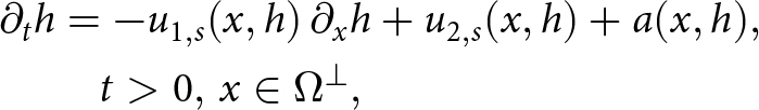
To compute the evolution of the ice surface function  $h=h(x,t)$ in time, we solve the free-surface equation:
 \begin{equation}
\begin{aligned}
\partial_t h &= - u_{1,s}(x,h)\, \partial_x h + u_{2,s}(x,h) + a(x,h),\\
&\quad t \gt 0,\, x \in \Omega^\perp,
\end{aligned}
\end{equation}
\begin{equation}
\begin{aligned}
\partial_t h &= - u_{1,s}(x,h)\, \partial_x h + u_{2,s}(x,h) + a(x,h),\\
&\quad t \gt 0,\, x \in \Omega^\perp,
\end{aligned}
\end{equation} where  $\Omega^\perp$ is a projected domain only taking into account the horizontal components of Ω. Furthermore,
  $u_{1,s}(x,h)$ and
  $u_{2,s}(x,h)$ are the surface horizontal and vertical velocity functions respectively. Term
  $a=a(x,h)$ is the surface mass balance in this paper set to
  $a(x,h) = 0$. We chose to work with the free-surface equation rather than the thickness equation (common when using the SIA models), as this allows for better flexibility in terms of using the free-surface equation discretizations already available from the existing full Stokes model codes such as Elmer or ISSM. The two equations can be derived one from another without any spurious residual terms. Their properties in terms of the largest feasible time step do not differ from an asymptotical perspective (comparing Cheng and others Reference Cheng, Lotstedt and von Sydow(2017) and Appendix A).
The evolution of the ice surface height h defines the evolution of shape of the domain Ω, where Ω is representing the volume of an ice sheet. The boundary of the domain 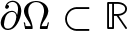 $\partial\Omega \subset \mathbb{R}$ consists of three disjoint parts:
 \begin{equation*}\partial\Omega = \Gamma_b \cup \Gamma_s \cup \Gamma_l ,\end{equation*}
 where  $\Gamma_b$ is the ice sheet bedrock,
  $\Gamma_s$ is the ice sheet free surface defined by the surface height h and
  $\Gamma_l$ is the ice sheet lateral boundary. A sketch of an ice sheet with the corresponding domain parts is given in Fig. 1.
A sketch representing the ice sheet boundary  $\partial\Omega$ subdivision into parts:
  $\Gamma_l$ (the two lateral boundaries),
  $\Gamma_s$ (the ice sheet free surface) and
  $\Gamma_b$ (the ice sheet bedrock).
As is observed from (1), the surface h is a function of the velocities u 1 and u 2. The velocities are computed before solving (1), by solving the momentum balance equations (SIA or Stokes) over Ω. The coupling between h, u 1 and u 2 has an important impact on the time-step restriction in the ice sheet simulations and is thus one of the main focus points of this paper.
When solving (1), we impose the boundary conditions as follows. We let the lateral margins of the ice sheet surface fixed and use either the periodic boundary conditions:
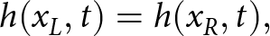 \begin{equation}
h(x_L,t) = h(x_R, t),
\end{equation}
\begin{equation}
h(x_L,t) = h(x_R, t),
\end{equation} where 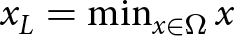 $x_L = \min_{x \in \Omega} x$ and
 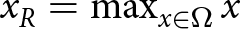 $x_R = \max_{x \in \Omega} x$ or Dirichlet boundary conditions:
 \begin{equation}
h(x_L, t) = 0,\quad h(x_R, t)=0.
\end{equation}
\begin{equation}
h(x_L, t) = 0,\quad h(x_R, t)=0.
\end{equation}This excludes influence from nonlinearities introduced by the moving lateral boundaries, which is a complex problem in itself (Werder and others, Reference Werder, Hewitt, Schoof and Flowers2013, Wirbel and Jarosch, Reference Wirbel and Jarosch2020, Bueler, Reference Bueler2023). The margins are sometimes fixed in practice for technical reasons, see some of the models in the ISMIP6 Antarctica benchmark (Seroussi and others, Reference Seroussi2020), but it is important to get the right physical response.
2.2. Strong form nonlinear full Stokes equations
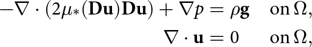
We use the full Stokes equations as a reference model for computing the velocity field 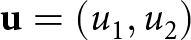 $\mathbf{u}=(u_1,u_2)$ over an ice sheet geometry, when drawing the comparison towards solutions of the different SIA model formulations. This is reasonable as the SIA model is an approximation of the full Stokes equations. The full Stokes equations are:
 \begin{equation}
\begin{aligned}
-\nabla \cdot \left(2 \mu_*(\mathbf{Du}) \mathbf{D}\mathbf{u} \right) + \nabla p &= \rho \mathbf{g} & \mathrm{on }\, \Omega,\\
\nabla \cdot \mathbf{u} &= 0& \mathrm{on }\, \Omega,
\end{aligned}
\end{equation}
\begin{equation}
\begin{aligned}
-\nabla \cdot \left(2 \mu_*(\mathbf{Du}) \mathbf{D}\mathbf{u} \right) + \nabla p &= \rho \mathbf{g} & \mathrm{on }\, \Omega,\\
\nabla \cdot \mathbf{u} &= 0& \mathrm{on }\, \Omega,
\end{aligned}
\end{equation} where ρ > 0 is the ice density,  $\mathbf{g}=(0,-9.81)\, {\mathrm{m }\mathrm{s}^{-2}}$ is the gravitational acceleration, p is the pressure and the symmetric strain rate tensor
  $\mathbf{D}\mathbf{u} = \frac{1}{2} \left (\nabla \mathbf{u} + \nabla \mathbf{u}^T \right )$ is defined through four components:
 \begin{equation}
\begin{aligned}
D_{11} &= \partial_x u_1,\quad D_{12} = \frac{1}{2}(\partial_y u_1 + \partial_x u_2), \\
\quad D_{21} &= D_{12}, \quad D_{22} = \partial_y u_2.
\end{aligned}
\end{equation}
\begin{equation}
\begin{aligned}
D_{11} &= \partial_x u_1,\quad D_{12} = \frac{1}{2}(\partial_y u_1 + \partial_x u_2), \\
\quad D_{21} &= D_{12}, \quad D_{22} = \partial_y u_2.
\end{aligned}
\end{equation} The viscosity function  $\mu_* = \mu_*(\mathbf{Du})$ relates the strain rates to the deviatoric stress tensor Su as
 \begin{equation}
\mathbf{Su}=2 \mu_*(\mathbf{D}\mathbf{u}) \mathbf{D}\mathbf{u},
\end{equation}
\begin{equation}
\mathbf{Su}=2 \mu_*(\mathbf{D}\mathbf{u}) \mathbf{D}\mathbf{u},
\end{equation}and is defined by:
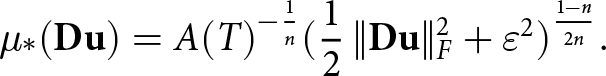 \begin{equation}
\mu_*(\mathbf{D} \mathbf{u}) = A(T)^{-\frac{1}{n}} (\frac{1}{2}\,\| \mathbf{D}\mathbf{u}\|_F^2 + {\varepsilon^2})^{\frac{1-n}{2n}}.
\end{equation}
\begin{equation}
\mu_*(\mathbf{D} \mathbf{u}) = A(T)^{-\frac{1}{n}} (\frac{1}{2}\,\| \mathbf{D}\mathbf{u}\|_F^2 + {\varepsilon^2})^{\frac{1-n}{2n}}.
\end{equation}Here n > 0 is Glen’s exponent (we use n = 3 throughout the paper), A(T) is constant since we consider isothermal conditions and ɛ is the regularization parameter (a small number) which we define as in Hirn Reference Hirn(2013).
In all the considered test cases, we impose stress-free boundary conditions 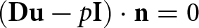 $(\mathbf{Du} - p\mathbf{I})\cdot \mathbf{n} = 0$ at the ice sheet surface
  $\Gamma_s$, where n is the normal vector pointing outwards of
  $\Gamma_s$. Depending on the test case, we impose either the periodic or the no-slip (
 $\mathbf{u} = \mathbf{0}$) boundary conditions over the ice sheet lateral boundary
  $\Gamma_l$. On the ice sheet bedrock
  $\Gamma_b$, we impose no-slip boundary conditions in all test cases.
In this paper, we use full Stokes equations written in weak form (abbreviated W-Stokes) defined later in the final paragraph of Section 2.5. The full Stokes equations are nonlinear which leads to an increase in computational cost when discretized and solved on a computer, as compared to a linear problem such as the SIA equations.
2.3. Strong form SIA equations (SIA)
The SIA model is derived by using that the normal stress deviators are negligible compared to vertical shear stress. Also, due to the disparity in the order of magnitudes of the spatial derivatives of velocity components, the horizontal derivative of the vertical velocity can be neglected. The stress tensor S as defined in (6) is then (Greve and Blatter, Reference Greve and Blatter2009):
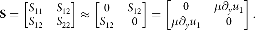 \begin{equation}
\mathbf{S}=\begin{bmatrix}
S_{11} & S_{12}\\
S_{12}& S_{22}
\end{bmatrix} \approx \begin{bmatrix}
0 & S_{12}\\
S_{12}& 0
\end{bmatrix} = \begin{bmatrix}
0 & \mu \partial_y u_1\\
\mu \partial_y u_1& 0
\end{bmatrix}.
\end{equation}
\begin{equation}
\mathbf{S}=\begin{bmatrix}
S_{11} & S_{12}\\
S_{12}& S_{22}
\end{bmatrix} \approx \begin{bmatrix}
0 & S_{12}\\
S_{12}& 0
\end{bmatrix} = \begin{bmatrix}
0 & \mu \partial_y u_1\\
\mu \partial_y u_1& 0
\end{bmatrix}.
\end{equation}The strong form SIA equations are:
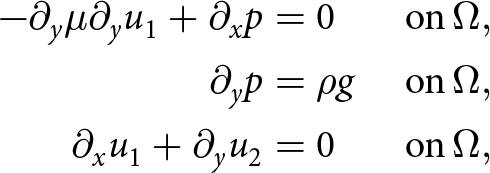 \begin{equation}
\begin{aligned}
- \partial_y \mu \partial_y u_1 + \partial_x p &= 0&\, \mathrm{on }\, \Omega, \\
\partial_y p &= \rho g&\, \mathrm{on }\, \Omega, \\
\partial_x u_1 + \partial_y u_2 &= 0&\, \mathrm{on }\, \Omega,
\end{aligned}
\end{equation}
\begin{equation}
\begin{aligned}
- \partial_y \mu \partial_y u_1 + \partial_x p &= 0&\, \mathrm{on }\, \Omega, \\
\partial_y p &= \rho g&\, \mathrm{on }\, \Omega, \\
\partial_x u_1 + \partial_y u_2 &= 0&\, \mathrm{on }\, \Omega,
\end{aligned}
\end{equation} where  $g = -9.81\, {\mathrm{m}\mathrm{s}^{-2}}$ is the second component of the gravity vector
  $\mathbf{g}$ defined in the scope of Section 2.2. The boundary conditions for (9) are:
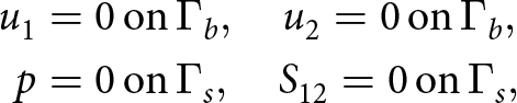 \begin{equation}
\begin{aligned}
u_1 &= 0\, \mathrm{on }\, \Gamma_b,\quad
u_2 = 0\, \mathrm{on }\, \Gamma_b,\quad \\
p &= 0\, \mathrm{on }\, \Gamma_s,\quad
S_{12} = 0 \, \mathrm{on }\, \Gamma_s,
\end{aligned}
\end{equation}
\begin{equation}
\begin{aligned}
u_1 &= 0\, \mathrm{on }\, \Gamma_b,\quad
u_2 = 0\, \mathrm{on }\, \Gamma_b,\quad \\
p &= 0\, \mathrm{on }\, \Gamma_s,\quad
S_{12} = 0 \, \mathrm{on }\, \Gamma_s,
\end{aligned}
\end{equation} where the different ice sheet domain parts are illustrated in Fig. 1. We let  $y \in [b(x), h(x)]$ be the vertical ice sheet coordinate, where b(x) and h(x) are the bedrock height and the free-surface height respectively, and where x is the horizontal coordinate of an ice sheet. As the pressure is decoupled from u 1 and u 2, we first solve the second equation of (9) for pressure. We vertically integrate the equation from y to h(x) and obtain:
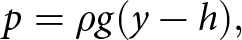 \begin{equation}
p=\rho g (y-h),
\end{equation}
\begin{equation}
p=\rho g (y-h),
\end{equation} where we additionally used that  $p(x,y=h)=0$. Inserting this hydrostatic pressure in the first equation of (9) and solving for
  $S_{12}=\mu \partial_y u_1$ using the vertical integration give:
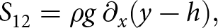 \begin{equation}
S_{12}=\rho g\, \partial_x (y-h),
\end{equation}
\begin{equation}
S_{12}=\rho g\, \partial_x (y-h),
\end{equation} where we also used that 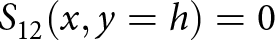 $S_{12}(x,y=h) = 0$. We then compute the SIA viscosity µ starting at the relation of fluidity (Greve and Blatter, Reference Greve and Blatter2009):
  $\mu^{-1} = 2 A(T) \sigma_e^{n-1} = 2 A(T) \|\mathbf{S}\|_F^{n-1}$. In the relation, we first use n = 3 and then
 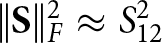 $\|\mathbf{S}\|_F^2 \approx S_{12}^2$ arising from (8). Simplifying
 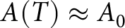 $A(T) \approx A_0$ and taking an inverse of the fluidity relation give
 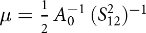 $\mu = \frac{1}{2}\, A_0^{-1}\, (S_{12}^{2})^{-1}$. Finally, inserting (12) gives the SIA viscosity:
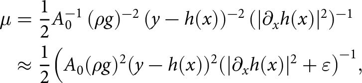 \begin{equation}
\begin{aligned}
\mu &= \frac{1}{2} A_0^{-1}\, (\rho g)^{-2}\, (y-h(x))^{-2}\, (|\partial_{x} h(x) |^{2})^{-1} \\
& \approx \frac{1}{2} \Big(A_0 (\rho g)^{2} (y-h(x))^{2} (|\partial_{x} h(x) |^2 + \varepsilon\big)^{-1},
\end{aligned}
\end{equation}
\begin{equation}
\begin{aligned}
\mu &= \frac{1}{2} A_0^{-1}\, (\rho g)^{-2}\, (y-h(x))^{-2}\, (|\partial_{x} h(x) |^{2})^{-1} \\
& \approx \frac{1}{2} \Big(A_0 (\rho g)^{2} (y-h(x))^{2} (|\partial_{x} h(x) |^2 + \varepsilon\big)^{-1},
\end{aligned}
\end{equation} where we have in the end also added Hirn’s regularization parameter preventing the viscosity from taking infinite values where  $|\partial_{x} h(x) |^2 \approx 0$. We observe that the SIA viscosity (13) only depends on y and h(x), but not on the velocity. To derive (13), we also assumed isothermal conditions
  $A(T) = A_0 = 100$
  $\mathrm{MPa}^{-3} \mathrm{yr}^{-1}$, where T is the temperature, but this is generally not a limitation of the SIA model. Using the viscosity function (13), the horizontal velocity u 1 is given by integrating the first equation of (9) along a vertical line from the bedrock height b(x) to y and inserting that
  $u_1|_{b(x)}=0$. The vertical velocity u 2 is obtained by inserting the computed u 1 into the third equation of (9), integrating over a vertical line from b(x) to y and inserting
  $u_2|_{b(x)}=0$. The closed-form expressions are:
 \begin{equation}
\begin{aligned}
u_1 &= - \frac{1}{2}A_0(\rho g)^3 (\partial_x h)^3 \left( (y-h)^4- (b-h)^4 \right)\\
u_2 &= \frac{1}{2}A_0\, (\rho g)^3 \\
&\quad \times \Bigg(\left(\frac{1}{5}(y-h)^5 - \frac{1}{5}(b-h)^5 - (b-h)^4\,(y-b)\right) \\
& \quad \times 3(\partial_x h)^2\, \partial_{xx} h + \cdots - (\partial_x h)^4\, ((y-h)^4 - (b-h)^4) \\
& \quad - 4 (\partial_x b - \partial_x h)\, (\partial_x h)^3 (b-h)^3\, \big((y-h) - (b-h) \big)\Bigg).
\end{aligned}
\end{equation}
\begin{equation}
\begin{aligned}
u_1 &= - \frac{1}{2}A_0(\rho g)^3 (\partial_x h)^3 \left( (y-h)^4- (b-h)^4 \right)\\
u_2 &= \frac{1}{2}A_0\, (\rho g)^3 \\
&\quad \times \Bigg(\left(\frac{1}{5}(y-h)^5 - \frac{1}{5}(b-h)^5 - (b-h)^4\,(y-b)\right) \\
& \quad \times 3(\partial_x h)^2\, \partial_{xx} h + \cdots - (\partial_x h)^4\, ((y-h)^4 - (b-h)^4) \\
& \quad - 4 (\partial_x b - \partial_x h)\, (\partial_x h)^3 (b-h)^3\, \big((y-h) - (b-h) \big)\Bigg).
\end{aligned}
\end{equation}These closed-form velocity expressions are computationally inexpensive to evaluate as compared to solving the full nonlinear Stokes system. The vertical integration, however, requires the mesh nodes to be aligned in the vertical direction in the case of adiabatic conditions, that is, when A varies with depth.
The free-surface equation requires the velocities to be evaluated at the surface. Setting y = h in (14) leads to:
 \begin{equation}
\begin{aligned}
u_{1,s} &= \frac{1}{2}A_0(\rho g)^3 (\partial_x h)^3 \left( (b-h)^4 \right)\\
u_{2,s} &= \frac{1}{2}A_0\, (\rho g)^3 \\
& \quad \times \Bigg(\Big(- \frac{3}{5}(b-h)^5 + 3(b-h)^5 \Big)\, (\partial_x h)^2\, \partial_{xx} h \\
& \quad + \Big(4(b-h)^4\, \partial_x b\, (\partial_x h)^2 - 3(b-h)^4(\partial_x h)^3 \Big)\, \partial_x h \Bigg).
\end{aligned}
\end{equation}
\begin{equation}
\begin{aligned}
u_{1,s} &= \frac{1}{2}A_0(\rho g)^3 (\partial_x h)^3 \left( (b-h)^4 \right)\\
u_{2,s} &= \frac{1}{2}A_0\, (\rho g)^3 \\
& \quad \times \Bigg(\Big(- \frac{3}{5}(b-h)^5 + 3(b-h)^5 \Big)\, (\partial_x h)^2\, \partial_{xx} h \\
& \quad + \Big(4(b-h)^4\, \partial_x b\, (\partial_x h)^2 - 3(b-h)^4(\partial_x h)^3 \Big)\, \partial_x h \Bigg).
\end{aligned}
\end{equation}The derivatives in this expression are evaluated by (i) interpolating the surface function onto a piecewise linear finite element space, (ii) taking a derivative within each element of a mesh and (iii) L 2-projecting the element-wise derivative back to the piecewise linear finite element space.
After inserting the SIA velocities from (14) to the free-surface Eqn. (1), we write the free-surface equation problem as a nonlinear advection-diffusion partial differential equation (PDE):
 \begin{equation}
\begin{aligned}
\partial_t h &= - u_{1,s}\,\partial_x h + u_{2,s}
= C_1(h)\, \partial_x h + C_2(h)\, \partial_{xx} h,
\end{aligned}
\end{equation}
\begin{equation}
\begin{aligned}
\partial_t h &= - u_{1,s}\,\partial_x h + u_{2,s}
= C_1(h)\, \partial_x h + C_2(h)\, \partial_{xx} h,
\end{aligned}
\end{equation}where:
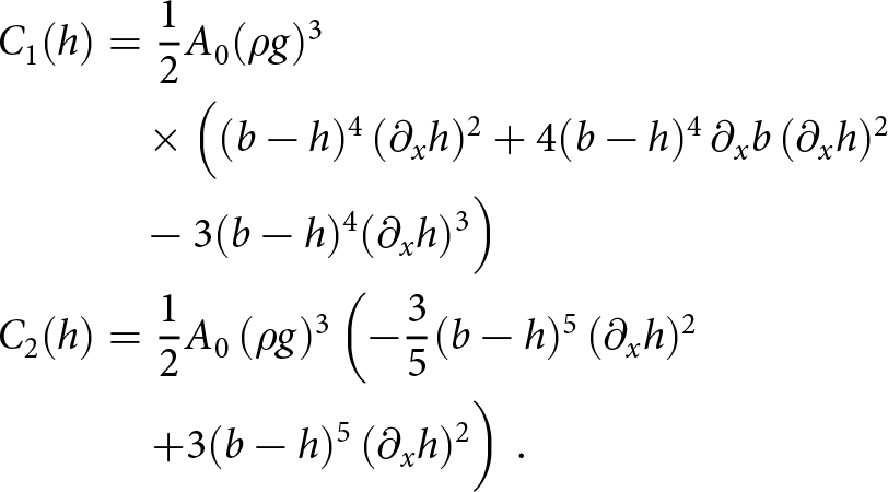 \begin{equation}
\begin{aligned}
C_1(h) &= \frac{1}{2}A_0(\rho g)^3 \\
& \quad \times \Big( (b-h)^4\, (\partial_x h)^2 + 4(b-h)^4\, \partial_x b\, (\partial_x h)^2 \\
& \quad -3(b-h)^4(\partial_x h)^3 \Big) \\
C_2(h) &= \frac{1}{2}A_0\, (\rho g)^3 \left(- \frac{3}{5}(b-h)^5\, (\partial_x h)^2 \right. \\
& \quad \left. + 3(b-h)^5\, (\partial_x h)^2 \vphantom{\left(- \frac{3}{5}(b-h)^5\, (\partial_x h)^2 \right.}\right)\, .
\end{aligned}
\end{equation}
\begin{equation}
\begin{aligned}
C_1(h) &= \frac{1}{2}A_0(\rho g)^3 \\
& \quad \times \Big( (b-h)^4\, (\partial_x h)^2 + 4(b-h)^4\, \partial_x b\, (\partial_x h)^2 \\
& \quad -3(b-h)^4(\partial_x h)^3 \Big) \\
C_2(h) &= \frac{1}{2}A_0\, (\rho g)^3 \left(- \frac{3}{5}(b-h)^5\, (\partial_x h)^2 \right. \\
& \quad \left. + 3(b-h)^5\, (\partial_x h)^2 \vphantom{\left(- \frac{3}{5}(b-h)^5\, (\partial_x h)^2 \right.}\right)\, .
\end{aligned}
\end{equation} The time-step restriction has a quadratic scaling in terms of the mesh size due to the second derivative term (diffusive term)  $\partial_{xx} h$ in (16). The standard way to theoretically assess the timestep restriction is to linearize (16) with respect to h and then perform a von Neumann (Fourier) analysis. This was done in, e.g., Cheng and others Reference Cheng, Lotstedt and von Sydow(2017) for the thickness equation in the case of a perturbed slab on a slope. We repeat this exercise for the free-surface equation in the appendix and will revisit it for a new SIA formulation where the FSSA stabilization of (Löfgren and others, Reference Löfgren, Ahlkrona and Helanow2022, Reference Lofgren, Zwinger, Raback, Helanow and Ahlkrona2023) is added.
2.4. Weak form SIA equations (W-SIA)
The easiest approach to implementing the SIA equations within an existing FEM code— such as Elmer, ISSM or FEniCS—is to write (9) in weak form and discretize the weak form using the standard FEMs. This also allows for fully unstructured meshes, which can be of higher quality on certain geometries, and is sometimes technically easier to construct. The weak SIA formulation is obtained by multiplying each equation of (9) using piecewise continuous test functions  $v_1=v_1(x,y),v_2=v_2(x,y)$,
 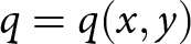 $q=q(x,y)$, respectively, and integrating over Ω. The first term of the first equation is additionally integrated by parts. In the end, the weak SIA formulation is:
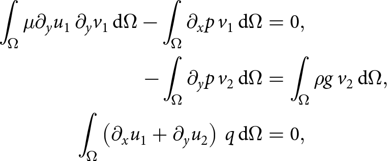 \begin{equation}
\begin{aligned}
\int_{\Omega} \mu \partial_y u_1\, \partial_y v_1\, \mathrm{d}\Omega - \int_\Omega \partial_x p\, v_1\, \mathrm{d}\Omega &= 0, \\
- \int_{\Omega} \partial_y p\, v_2\, \mathrm{d}\Omega &= \int_\Omega \rho g\, v_2\, \mathrm{d}\Omega, \\
\int_\Omega \left(\partial_x u_1 + \partial_y u_2\right)\, q\, \mathrm{d}\Omega &= 0,
\end{aligned}
\end{equation}
\begin{equation}
\begin{aligned}
\int_{\Omega} \mu \partial_y u_1\, \partial_y v_1\, \mathrm{d}\Omega - \int_\Omega \partial_x p\, v_1\, \mathrm{d}\Omega &= 0, \\
- \int_{\Omega} \partial_y p\, v_2\, \mathrm{d}\Omega &= \int_\Omega \rho g\, v_2\, \mathrm{d}\Omega, \\
\int_\Omega \left(\partial_x u_1 + \partial_y u_2\right)\, q\, \mathrm{d}\Omega &= 0,
\end{aligned}
\end{equation}where µ is the SIA viscosity defined in (13). In this paper, we abbreviate the weak SIA formulation as W-SIA. Solving W-SIA on a computer is cheaper as compared to solving the full nonlinear Stokes system (4), since W-SIA is a linear problem due to that the viscosity is not a function of the computed velocity. W-SIA is possible to solve in terms of three subsequent matrix systems: first for pressure, second for u 1 and last for u 2. This only holds as long as W-SIA is not further stabilized using the additional stabilization terms that couple the velocity functions. A disadvantage when solving W-SIA is that the many stress components are not present in (18). This implies that the full stress term Su is not guaranteed to have an upper bound when the problem is solved on a computer and the mesh size approaches zero. A consequence is potentially sharp velocity gradients that deteriorate the numerical stability as well as the solution accuracy.
Under the assumption that the PDE data are regular enough, the solution to the weak formulation is identical to that of the strong formulation. However, we do not expect this to be true numerically across W-SIA (18) and SIA (9), as the surface derivatives in the closed-form SIA solution (15) are evaluated numerically. The differences across the solutions are highly dependent on the choice of the numerical evaluation of the derivatives. This is also a potential source of the differences across the two formulations in the largest feasible time step when using the velocities to advance the surface function in time.
2.5. Weak form linear Stokes equations employing the SIA viscosity function (W-SIAStokes)
We add the missing stress components back to (18) resulting in the following weak formulation:
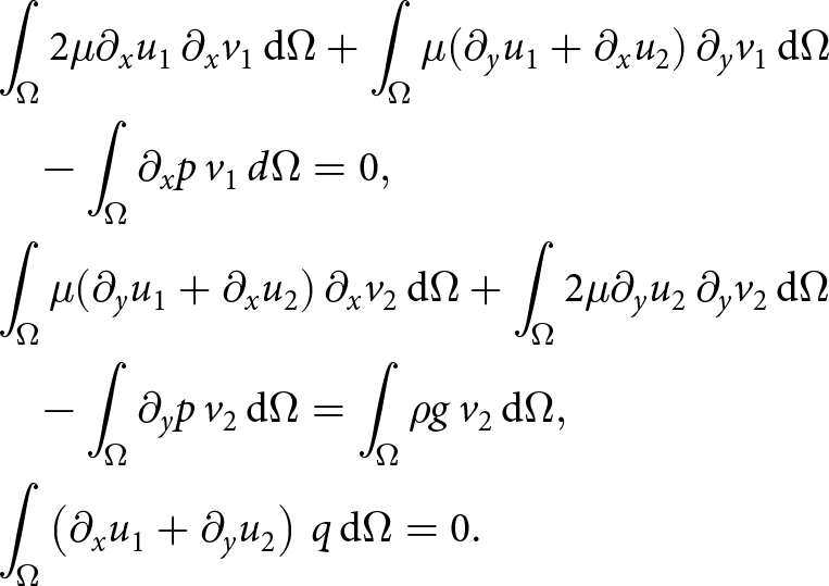 \begin{equation}
\begin{aligned}
&\int_{\Omega} 2\mu \partial_x u_1\, \partial_x v_1\, \mathrm{d}\Omega + \int_{\Omega} \mu (\partial_y u_1 + \partial_x u_2)\, \partial_y v_1\, \mathrm{d}\Omega \\
& \quad - \int_\Omega \partial_x p\, v_1\, d\Omega = 0, \\
&\int_{\Omega} \mu (\partial_y u_1 + \partial_x u_2)\, \partial_x v_2\, \mathrm{d}\Omega + \int_{\Omega} 2\mu \partial_y u_2\, \partial_y v_2\, \mathrm{d}\Omega \\
& \quad - \int_{\Omega} \partial_y p\, v_2\, \mathrm{d}\Omega = \int_\Omega \rho g\, v_2\, \mathrm{d}\Omega, \\
&\int_\Omega \left(\partial_x u_1 + \partial_y u_2\right)\, q\, \mathrm{d}\Omega = 0.
\end{aligned}
\end{equation}
\begin{equation}
\begin{aligned}
&\int_{\Omega} 2\mu \partial_x u_1\, \partial_x v_1\, \mathrm{d}\Omega + \int_{\Omega} \mu (\partial_y u_1 + \partial_x u_2)\, \partial_y v_1\, \mathrm{d}\Omega \\
& \quad - \int_\Omega \partial_x p\, v_1\, d\Omega = 0, \\
&\int_{\Omega} \mu (\partial_y u_1 + \partial_x u_2)\, \partial_x v_2\, \mathrm{d}\Omega + \int_{\Omega} 2\mu \partial_y u_2\, \partial_y v_2\, \mathrm{d}\Omega \\
& \quad - \int_{\Omega} \partial_y p\, v_2\, \mathrm{d}\Omega = \int_\Omega \rho g\, v_2\, \mathrm{d}\Omega, \\
&\int_\Omega \left(\partial_x u_1 + \partial_y u_2\right)\, q\, \mathrm{d}\Omega = 0.
\end{aligned}
\end{equation}We abbreviate (19) as W-SIAStokes, as that formulation combines the full Stokes problem and the SIA viscosity function. W-SIAStokes is a linear problem, computationally less expensive to solve as compared to the full nonlinear Stokes problem. However, the system can no longer be solved as three separate matrix systems as is the case in the unstabilized W-SIA formulation (18). An advantage of W-SIAStokes over W-SIA is a guaranteed bound over the full stress term Su, which improves the numerical stability properties as the mesh size goes to 0.
We note that the nonlinear full Stokes problem (4) but written in weak form (W-Stokes) takes exactly the same form as W-SIAStokes (19), where we use the (full) viscosity function (7) instead of the SIA viscosity (13).
3. Finite difference discretization of the free-surface equation
We first denote that  $h=h(x,t)$ and discretize the free-surface Eqn. (1) in time using the first order semi-implicit Euler method. This results in:
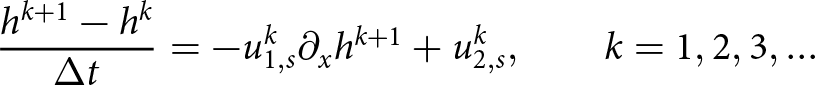 \begin{equation}
\frac{h^{k+1} - h^k}{\Delta t } = - u_{1,s}^k \partial_x h^{k+1} + u_{2,s}^k,\qquad k=1,2,3,\ldots
\end{equation}
\begin{equation}
\frac{h^{k+1} - h^k}{\Delta t } = - u_{1,s}^k \partial_x h^{k+1} + u_{2,s}^k,\qquad k=1,2,3,\ldots
\end{equation} where  $h^k, h^{k+1}$ are
  $h(x,t_k)$,
  $h(x,t_{k+1})$ respectively, and where
  $u_{1,s}^k$,
  $u_{2,s}^k$ are the surface velocities
  $u_1(x^k,y_s^k)$,
  $u_2(x^k,y_s^k)$ extracted from the bulk velocity functions defined over an ice sheet domain
  $\Omega^k$ at tk. We note that
  $x \in \Omega^\perp$, where this domain is defined in the scope of Section 2.1. Now we discretize the spatial derivatives in (20) using the second-order accurate centred finite difference stencil weights, resulting in the following system of equations:
 \begin{equation}
\frac{\mathbf{h}^{k+1} - \mathbf{h}^k}{\Delta t } = - \mathrm{diag}(\mathbf{u}_{1,s}^k) \mathbf{D}_x \mathbf{h}^{k+1} + \mathbf{u}_{2,s}^k,\qquad k=1,2,3,\ldots
\end{equation}
\begin{equation}
\frac{\mathbf{h}^{k+1} - \mathbf{h}^k}{\Delta t } = - \mathrm{diag}(\mathbf{u}_{1,s}^k) \mathbf{D}_x \mathbf{h}^{k+1} + \mathbf{u}_{2,s}^k,\qquad k=1,2,3,\ldots
\end{equation} where  $h^{k+1}_i = h(x_i,t_{k+1})$,
  $h^{k}_i = h(x_i,t_{k})$,
  $(u_1^{k+1})_i = u_1(x_i, y_s)$,
  $(u_2^{k+1})_i = u_2(x_i, y_s)$,
  $i=1,\ldots,N$. The components of the matrix
  $\mathbf{D}_x$ are defined by the second-order accurate finite difference stencil weights that discretize the first-order derivative operator. The final time-stepping iteration scheme is:
 \begin{equation}
\mathbf{h}^{k+1} = (\mathbf{I} + \Delta t\, \mathrm{diag}(\mathbf{u}_{1,s}^k) \mathbf{D}_x)^{-1}\, (\mathbf{h}^k + \Delta t\,\mathbf{u}_{2,s}^k),\qquad k=1,2,3,\ldots.
\end{equation}
\begin{equation}
\mathbf{h}^{k+1} = (\mathbf{I} + \Delta t\, \mathrm{diag}(\mathbf{u}_{1,s}^k) \mathbf{D}_x)^{-1}\, (\mathbf{h}^k + \Delta t\,\mathbf{u}_{2,s}^k),\qquad k=1,2,3,\ldots.
\end{equation} We impose the boundary conditions as described within the scope of Section 2.1 by reducing the system of equations (22) in the unknowns related to the Dirichlet conditions or by transforming the  $\mathbf{D}_x$ matrix into a circulant matrix in the case when we use the periodic boundary conditions.
Using a fully implicit scheme would require access to  $u_1^{k+1}$,
  $u_2^{k+1}$, but this is computationally expensive as the velocity functions and the surface position are coupled. The surface h depends on
  $u_1^{k+1}$,
  $u_2^{k+1}$ due to (20), while the velocities depend on the surface that determines the shape of the computational domain Ω on which we solve the momentum balance equations. As a consequence, computing
  $u_1^{k+1}$,
  $u_2^{k+1}$ requires an expensive nonlinear iteration as demonstrated in the SIA model case in Bueler Reference Bueler(2016).
4. Finite element discretization of the SIA/Stokes models
Throughout the paper, we use FEM not only to solve partial differential equations in weak form but also to evaluate the surface gradient functions. The meshes we use are extruded. To create a 2-D ice sheet mesh, we first generate a rectangular mesh with dimensions  $[x_{\mathrm{min}}, x_{\mathrm{max}}] \times [0, 1]$, where
  $x_{\mathrm{min}}$ and
  $x_{\mathrm{max}}$ are the minimum and maximum horizontal coordinates of the ice sheet geometry. Then we transform the vertical mesh coordinates using an ice sheet initial surface function.
When evaluating the SIA velocities using the closed-form expression (14), we employ FEM to evaluate  $\partial_x h$, the gradient of the ice sheet surface. We first interpolate h into a piecewise linear finite element space. After that, we compute the gradient
  $\partial_x h|_{K_i}$,
  $i=1,\ldots,N$ over each mesh element Ki. As the gradient of the piecewise linear function across the element interfaces is discontinuous (not well defined), we L 2 project the computed gradients back into a piecewise linear finite element space. By that, we compute a continuous (well-defined) surface gradient.
When solving the nonlinear Stokes problem (4) in the weak form, we use Taylor–Hood elements (P2P1) to fulfil the inf-sup condition (Babuska, Reference Babuska1973, Brezzi, Reference Brezzi1974), that is, piecewise quadratic polynomials for approximating the velocity functions and piecewise linear polynomials for approximating the pressure function. This is a requirement to make the finite element discretization numerically stable.
When solving W-SIAStokes (19), we use the same type of elements as in the nonlinear Stokes problem case, for the very same reasons related to numerical stability.
When solving W-SIA the inf-sup condition does not need to be fulfilled, and we can therefore use piecewise linear finite elements (P1P1) for approximating the velocity functions as well as the pressure function. This is an advantage as the amount of unknowns when using P1P1 elements is smaller as compared to when using P2P1 elements. This is attributed to the fact that P2 finite element spaces require an addition of three midpoints over the edges of a triangle in a mesh, which then increases the total count of the degrees of freedom.
5. FSSA for the SIA/Stokes models
In Löfgren and others (Reference Löfgren, Ahlkrona and Helanow2022, Reference Lofgren, Zwinger, Raback, Helanow and Ahlkrona2023), the authors introduced FSSA for the full nonlinear Stokes model to mimic an associated implicit solver advancing the ice surface from time tk to time  $t_{k+1}$,
 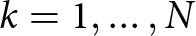 $k=1,\ldots,N$, where
  $t_{k+1} \gt t_k$. This is done by predicting the gravitational force in the weak form at
  $t_{k+1}$ by adding an extra surface force term:
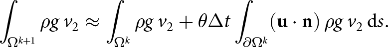 \begin{equation}
\int_{\Omega^{k+1}} \rho g\, v_2 \approx \int_{\Omega^{k}} \rho g\, v_2 + \theta \Delta t \int_{\partial \Omega^k} (\mathbf{u \cdot n})\, \rho g\, v_2\, \mathrm{d}s.
\end{equation}
\begin{equation}
\int_{\Omega^{k+1}} \rho g\, v_2 \approx \int_{\Omega^{k}} \rho g\, v_2 + \theta \Delta t \int_{\partial \Omega^k} (\mathbf{u \cdot n})\, \rho g\, v_2\, \mathrm{d}s.
\end{equation} Here  $\theta \in [0,1]$ is a user-defined constant parameter. The relation (23) was derived from a finite difference discretization of the Reynolds transport theorem (the multi-dimensional Leibniz rule). The FSSA thus relies on the assumption that the flow is predominantly gravity-driven so that computing the gravitational force at
  $t_{k+1}$ leads to a good approximation of the ice flow at
  $t_{k+1}$. This, in turn, enables taking larger time steps when solving the free-surface equation. Hence it is an implicit discretization (Löfgren and others, Reference Löfgren, Ahlkrona and Helanow2022, Reference Lofgren, Zwinger, Raback, Helanow and Ahlkrona2023). From a physics standpoint, the FSSA term is an extra surface pressure term acting as a damping term—when the ice is rising, the FSSA term acts as an extra surface pressure, and when the ice is sinking, it reduces the pressure. FSSA was originally introduced by Kaus and others Reference Kaus, Mühlhaus and May(2010) for mantle convection simulations.
In this paper, we add the FSSA stabilization term to the vertical momentum balance equation. In the W-SIAStokes case (19) (and similar in the W-Stokes case), the vertical momentum balance equation becomes:
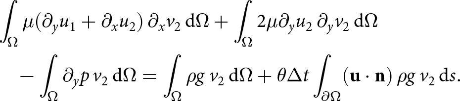 \begin{equation}
\begin{aligned}
&\int_{\Omega} \mu (\partial_y u_1 + \partial_x u_2)\, \partial_x v_2\, \mathrm{d}\Omega + \int_{\Omega} 2\mu \partial_y u_2\, \partial_y v_2\, \mathrm{d}\Omega \\
& \quad - \int_{\Omega} \partial_y p\, v_2\, \mathrm{d}\Omega = \int_\Omega \rho g\, v_2\, \mathrm{d}\Omega + \theta \Delta t \int_{\partial\Omega} (\mathbf{u \cdot n})\, \rho g\, v_2\, \mathrm{d}s.
\end{aligned}
\end{equation}
\begin{equation}
\begin{aligned}
&\int_{\Omega} \mu (\partial_y u_1 + \partial_x u_2)\, \partial_x v_2\, \mathrm{d}\Omega + \int_{\Omega} 2\mu \partial_y u_2\, \partial_y v_2\, \mathrm{d}\Omega \\
& \quad - \int_{\Omega} \partial_y p\, v_2\, \mathrm{d}\Omega = \int_\Omega \rho g\, v_2\, \mathrm{d}\Omega + \theta \Delta t \int_{\partial\Omega} (\mathbf{u \cdot n})\, \rho g\, v_2\, \mathrm{d}s.
\end{aligned}
\end{equation}In the W-SIA case (18), the vertical momentum balance, after adding the FSSA stabilization term, becomes:
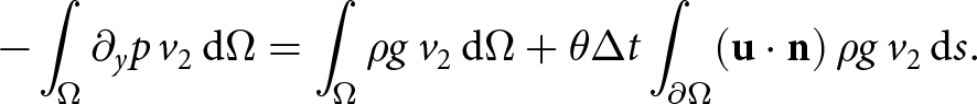 \begin{equation}
- \int_{\Omega} \partial_y p\, v_2\, \mathrm{d}\Omega = \int_\Omega \rho g\, v_2\, \mathrm{d}\Omega + \theta \Delta t \int_{\partial\Omega} (\mathbf{u \cdot n})\, \rho g\, v_2\, \mathrm{d}s.
\end{equation}
\begin{equation}
- \int_{\Omega} \partial_y p\, v_2\, \mathrm{d}\Omega = \int_\Omega \rho g\, v_2\, \mathrm{d}\Omega + \theta \Delta t \int_{\partial\Omega} (\mathbf{u \cdot n})\, \rho g\, v_2\, \mathrm{d}s.
\end{equation}In this case, it is the added FSSA term that couples the pressure to surface velocities us. Without the FSSA term, the pressure is decoupled from the velocity, reducing the computational cost of the solution procedure. The coupling is, however, essential for numerical stability reasons.
5.1. Effects of the added FSSA terms on W-SIA
The FSSA term is using the discretized free-surface equation (22) to estimate how the force of gravity will change between times tk and  $t_{k+1}$. The argumentation is provided as follows. Assume the domain Ω is such that the horizontal and vertical integration can be separated, i.e.
  $\int_{\Omega} (\cdot) \mathrm{d}\Omega=\int_{\Omega^\perp} \int_y (\cdot) \mathrm{d}y\, \mathrm{d}x$, where
  $\Omega^\perp$ only contains the horizontal coordinates of Ω and is defined in the scope of (1). Then the vertical momentum equation (25), after setting θ = 1, becomes:
 \begin{equation}
\begin{aligned}
- \int_{\Omega^\perp} \int_b^{h^k} \partial_y p\, v_2\, \mathrm{d}y\, \mathrm{d}x &= \int_{\Omega^\perp} \int_b^{h^k} \rho g\, v_2\, \mathrm{d}y\, \mathrm{d}x \\
&\quad + \Delta t \int_{\Gamma_s^k} (\mathbf{u \cdot n})\, \rho g\, v_2\, \mathrm{d}s.
\end{aligned}
\end{equation}
\begin{equation}
\begin{aligned}
- \int_{\Omega^\perp} \int_b^{h^k} \partial_y p\, v_2\, \mathrm{d}y\, \mathrm{d}x &= \int_{\Omega^\perp} \int_b^{h^k} \rho g\, v_2\, \mathrm{d}y\, \mathrm{d}x \\
&\quad + \Delta t \int_{\Gamma_s^k} (\mathbf{u \cdot n})\, \rho g\, v_2\, \mathrm{d}s.
\end{aligned}
\end{equation} As the normal vector and the arc length of a surface are, respectively, defined as  $\mathbf{n}=(-\partial_x h, 1)/\sqrt{\partial_x h)^2+1^2}$ and
  $\mathrm{d}s=\sqrt{\partial_x h)^2+1^2}\,dx$, we have that
  $(\mathbf{u} \cdot \mathbf{n})\, \mathrm{d}s = (- u_{1,s}\partial_x h + u_{2,s})\, \mathrm{d}x$. Using that, and (20) to make an additional relation to the discretized free-surface equation, we write the FSSA term in (26) as:
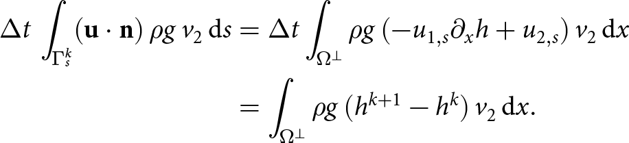 \begin{equation}
\begin{aligned}
\Delta t\, \int_{\Gamma_s^k} (\mathbf{u \cdot n})\, \rho g\, v_2\, \mathrm{d}s &= \Delta t \int_{\Omega^\perp}\rho g\, (- u_{1,s}\partial_x h + u_{2,s})\, v_2\, \mathrm{d}x \\
&= \int_{\Omega^\perp}\rho g\, (h^{k+1} - h^k)\, v_2\, \mathrm{d}x.
\end{aligned}
\end{equation}
\begin{equation}
\begin{aligned}
\Delta t\, \int_{\Gamma_s^k} (\mathbf{u \cdot n})\, \rho g\, v_2\, \mathrm{d}s &= \Delta t \int_{\Omega^\perp}\rho g\, (- u_{1,s}\partial_x h + u_{2,s})\, v_2\, \mathrm{d}x \\
&= \int_{\Omega^\perp}\rho g\, (h^{k+1} - h^k)\, v_2\, \mathrm{d}x.
\end{aligned}
\end{equation} We now look at the expression  $\left(h^{k+1}-h^k\right) v_2$ as a left point rule approximation of the integral
  $\int_{h^k}^{h^{k+1}} v_2\,dy$. Then we have
  $\int_{\Omega^\perp}\rho g\, (h^{k+1} - h^k)\, v_2\, \mathrm{d}x \approx
\int_{\Omega^\perp} \int_{h^k}^{h^{k+1}} \rho g\, v_2\, \mathrm{d}y\, \mathrm{d}x$. Combining this with (27) and then with (26), we obtain:
$\int_{\Omega^\perp}\rho g\, (h^{k+1} - h^k)\, v_2\, \mathrm{d}x \approx
\int_{\Omega^\perp} \int_{h^k}^{h^{k+1}} \rho g\, v_2\, \mathrm{d}y\, \mathrm{d}x$. Combining this with (27) and then with (26), we obtain:
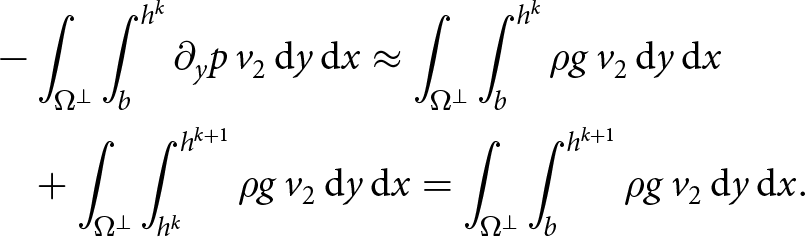 \begin{equation}
\begin{aligned}
&- \int_{\Omega^\perp} \int_b^{h^k} \partial_y p\, v_2\, \mathrm{d}y\, \mathrm{d}x \approx \int_{\Omega^\perp} \int_b^{h^k} \rho g\, v_2\, \mathrm{d}y\, \mathrm{d}x \\
& \quad + \int_{\Omega^\perp} \int_{h^k}^{h^{k+1}} \rho g\, v_2\, \mathrm{d}y\, \mathrm{d}x = \int_{\Omega^\perp} \int_b^{h^{{k+1}}} \rho g\, v_2\, \mathrm{d}y\, \mathrm{d}x.
\end{aligned}
\end{equation}
\begin{equation}
\begin{aligned}
&- \int_{\Omega^\perp} \int_b^{h^k} \partial_y p\, v_2\, \mathrm{d}y\, \mathrm{d}x \approx \int_{\Omega^\perp} \int_b^{h^k} \rho g\, v_2\, \mathrm{d}y\, \mathrm{d}x \\
& \quad + \int_{\Omega^\perp} \int_{h^k}^{h^{k+1}} \rho g\, v_2\, \mathrm{d}y\, \mathrm{d}x = \int_{\Omega^\perp} \int_b^{h^{{k+1}}} \rho g\, v_2\, \mathrm{d}y\, \mathrm{d}x.
\end{aligned}
\end{equation}Rewriting the double integration in the equation above back to integration over Ω and inserting that to the FSSA-stabilized vertical momentum balance (25), we have that:
 \begin{equation}
\begin{aligned}
- \int_{\Omega^k} \partial_y p\, v_2\, \mathrm{d}\Omega &= \int_{\Omega^k} \rho g\, v_2\, \mathrm{d}\Omega + \Delta t \int_{\partial\Omega^k} (\mathbf{u} \cdot \mathbf{n})\, \rho g\, v_2\, \mathrm{d}s \\
&\approx \int_{\Omega^{k+1}} \rho g\, v_2\, \mathrm{d}\Omega.
\end{aligned}
\end{equation}
\begin{equation}
\begin{aligned}
- \int_{\Omega^k} \partial_y p\, v_2\, \mathrm{d}\Omega &= \int_{\Omega^k} \rho g\, v_2\, \mathrm{d}\Omega + \Delta t \int_{\partial\Omega^k} (\mathbf{u} \cdot \mathbf{n})\, \rho g\, v_2\, \mathrm{d}s \\
&\approx \int_{\Omega^{k+1}} \rho g\, v_2\, \mathrm{d}\Omega.
\end{aligned}
\end{equation} The left-hand-side integral of (29) is integrated over  $\Omega^k$. However, we observe that the addition of the FSSA terms implies that the right-hand-side forcing term of (29) is integrated over
  $\Omega^{k+1}$ in place of
  $\Omega^k$. Thus, we expect that the solution p from (29) is approximated at time
  $t_{k+1}$. When this p is used to compute the velocity in (18), we expect the computed velocities to also be approximated at time
  $t_{k+1}$. Using such velocities when advancing the free surface in time through (22) renders an approximately implicit time stepping treatment, which in turn allows taking larger time steps. A more precise observation on this effect is given for the strong form SIA model, which is the focus of the next section.
5.2. Stability analysis of SIA combined with FSSA
In the following section, we show how a strong form version of the FSSA terms impacts numerical stability of SIA. The strong setting allows us to derive formulas for the FSSA-stabilized pressure and also for Fourier analysis. We note that the analysis is meant to give a better insight into how FSSA works. The results, however, cannot be directly transferred to the weak setting.
We construct a strong form of FSSA for the strong SIA vertical momentum equation (9). We do that by starting at the SIA pressure (11) evaluated at tk, and then adding a scaled normal velocity term, inspired by the FSSA stabilization term in (25). We have:
 \begin{equation}
p_*^k = \rho g (y - h^k) - \Delta t\, \rho g\, (\mathbf{u} \cdot \mathbf{n})|_{y=h^k(x)}.
\end{equation}
\begin{equation}
p_*^k = \rho g (y - h^k) - \Delta t\, \rho g\, (\mathbf{u} \cdot \mathbf{n})|_{y=h^k(x)}.
\end{equation} Assuming that the free surface is close to flat we have that  $(\partial_x h)^2 \approx 0$ (equivalent to
  $(\partial_x h)^2 \ll 1$). The surface normal is then
  $\mathbf{n}=(-\partial_x h, 1)/\sqrt{(\partial_x h)^2+1^2} \approx (-\partial_x h, 1)$. Using this in (30), we have:
 \begin{equation}
p_*^k \approx \rho g\, (y - h^k) - \Delta t\, \rho g\, (- u_{1,s}\, \partial_x h + u_{2,s}).
\end{equation}
\begin{equation}
p_*^k \approx \rho g\, (y - h^k) - \Delta t\, \rho g\, (- u_{1,s}\, \partial_x h + u_{2,s}).
\end{equation}Using (22) on the second term of the right-hand side of equation above, we arrive at:
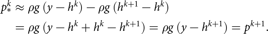 \begin{equation}
\begin{aligned}
p_*^k &\approx \rho g\, (y - h^k) - \rho g\, (h^{k+1} - h^k) \\
&= \rho g\, (y - h^k + h^k - h^{k+1}) = \rho g\,(y - h^{k+1}) = p^{k+1}.
\end{aligned}
\end{equation}
\begin{equation}
\begin{aligned}
p_*^k &\approx \rho g\, (y - h^k) - \rho g\, (h^{k+1} - h^k) \\
&= \rho g\, (y - h^k + h^k - h^{k+1}) = \rho g\,(y - h^{k+1}) = p^{k+1}.
\end{aligned}
\end{equation} Hence, the FSSA-inspired correction to the SIA pressure in (30) contributes to approximating pressure at time  $t^{k+1}$. In Appendix A, we perform the Fourier analysis to show that when using
  $p^{k+1}$ to compute the strong SIA velocities (i.e. using an implicit representation of the pressure) is enough to alleviate the quadratic time-step restriction
  $\Delta t \lt C \Delta x^2$ when solving the free-surface equation. To derive this result, we extended the von Neumann type analysis for a slab on a slope test case from (Cheng and others, Reference Cheng, Lotstedt and von Sydow2017). In Cheng and others Reference Cheng, Lotstedt and von Sydow(2017), the authors show that, assuming thick ice with low surface inclination, the quadratic dependence on
  $\Delta x$ is:
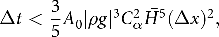 \begin{equation}
\Delta t \lt \frac{3}{5}A_0 |\rho g|^3 C_\alpha^2 \bar{H}^5 (\Delta x)^2,
\end{equation}
\begin{equation}
\Delta t \lt \frac{3}{5}A_0 |\rho g|^3 C_\alpha^2 \bar{H}^5 (\Delta x)^2,
\end{equation} where Cα is the average surface slope and H the ice thickness. The result stems from that the vertical velocity u 2 contains a second derivative of the surface  $\partial_{xx} h$. Furthermore, the second derivative of the surface origins from the vertical velocity is a function of
  $\partial_x u_1$, which is in turn a function of the horizontal pressure derivative
 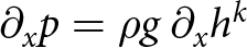 $\partial_x p= \rho g\, \partial_x h^k$. Following the derivation of the compact form free-surface equation (16) with the coefficients (17), we now write the time discretized free-surface equation when assuming that the velocities are derived from
  $p^{k+1}$, but that the intermediate integration steps involve hk. We have:
 \begin{equation}
h^{k+1} = h^k + C_0\, \partial_x h^{k} + C_1\, \partial_x h^{k+1} + C_2\, \partial_{xx} h^{k+1}
\end{equation}
\begin{equation}
h^{k+1} = h^k + C_0\, \partial_x h^{k} + C_1\, \partial_x h^{k+1} + C_2\, \partial_{xx} h^{k+1}
\end{equation}where:
 \begin{equation}
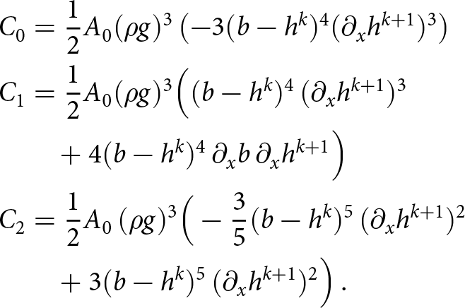
\begin{aligned}
C_0 &= \frac{1}{2}A_0(\rho g)^3 \left( - 3(b-h^k)^4(\partial_x h^{k+1})^3 \right) \\
C_1 &= \frac{1}{2}A_0(\rho g)^3 \Big( (b-h^k)^4\, (\partial_x h^{k+1})^3 \\
& \quad + 4(b-h^k)^4\, \partial_x b\, \partial_x h^{k+1} \Big ) \\
C_2 &= \frac{1}{2}A_0\, (\rho g)^3 \Big(- \frac{3}{5}(b-h^k)^5\, (\partial_x h^{k+1})^2 \\
& \quad + 3(b-h^k)^5\, (\partial_x h^{k+1})^2 \Big)\, .
\end{aligned}
\end{equation}
\begin{equation}
\begin{aligned}
C_0 &= \frac{1}{2}A_0(\rho g)^3 \left( - 3(b-h^k)^4(\partial_x h^{k+1})^3 \right) \\
C_1 &= \frac{1}{2}A_0(\rho g)^3 \Big( (b-h^k)^4\, (\partial_x h^{k+1})^3 \\
& \quad + 4(b-h^k)^4\, \partial_x b\, \partial_x h^{k+1} \Big ) \\
C_2 &= \frac{1}{2}A_0\, (\rho g)^3 \Big(- \frac{3}{5}(b-h^k)^5\, (\partial_x h^{k+1})^2 \\
& \quad + 3(b-h^k)^5\, (\partial_x h^{k+1})^2 \Big)\, .
\end{aligned}
\end{equation} We now have an implicit treatment of the leading diffusive  $\partial_{xx} h$ term in (34) which leads to a linear time-step constraint:
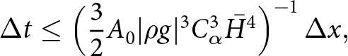 \begin{equation}
\Delta t \leq \Big(\frac{3}{2}A_0 |\rho g|^3 C_\alpha^3 \bar{H}^4 \Big)^{-1}\, \Delta x,
\end{equation}
\begin{equation}
\Delta t \leq \Big(\frac{3}{2}A_0 |\rho g|^3 C_\alpha^3 \bar{H}^4 \Big)^{-1}\, \Delta x,
\end{equation}where Cα is the average surface slope. We derive the above time-step restriction for the slab on a slope with a perturbed ice surface case in Appendix A and validate the estimate numerically for W-SIA and W-SIAStokes in the numerical experiments section.
6. Computational cost estimation for the different SIA/Stokes formulations
The computational work when solving momentum balance models is highly dependent on both software and hardware. However, it is still possible to make estimates of the computational cost, for instance, a type of performance analysis approach of Bueler Reference Bueler(2023). In this section, we make rough estimates of the computational cost for ice sheet simulations, where the velocity functions are computed using SIA (9), W-SIA (18), W-SIAStokes (19) and W-Stokes (7), and the ice surface is advanced from time tk to time  $t_{k+1}$,
  $k=1,\ldots,N_{\Delta t}$, using the discretized free-surface equation (22). We write the approximate computational cost on the form:
 \begin{equation*}\mathrm{Computational\,cost} = C(d,\alpha)\, C_S\, m^{1 + \gamma/(d-1) + \alpha },\end{equation*}
where:
• m is the number of mesh vertices (nodes) in the horizontal direction,
•
$\alpha \in [0, 2]$ denotes the choice of a linear solver (α = 2 dense direct solver, α = 1 sparse direct solver, α = 0.05 algebraic multigrid solver (Bueler, Reference Bueler2023)). For pure SIA, no linear solver is needed and α = 0.• γ is the scaling exponent in the simulation time-step restriction
$\Delta t \leq C_t\, \Delta x^\gamma$, where
$\Delta x$ is the horizontal internodal distance.• CS is a constant specific to the computational cost of the nonlinear Stokes problem which involves the nonlinear iteration count and the choice of hardware,
•
$C(d,\alpha)$ is a constant depending on α and d, where d is the dimension count of the considered ice sheet geometry.


Following Bueler Reference Bueler(2023), we have that W-Stokes requires  $C_{S}\, m^{1+\alpha}$ floating point operations until convergence per one time step.
In the W-SIAStokes case, the computational cost is the same as in W-Stokes but divided by the nonlinear iteration count  $N_{\mathrm{iter}}$. The cost is
 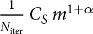 $\frac{1}{N_{\mathrm{iter}}}\, C_{S}\, m^{1+\alpha}$. This is due to that W-SIAStokes only differs from W-SIA in the choice of the viscosity function (linear) (13) and thus requires one iteration to be solved. When making the estimate we also assumed that the different viscosity function preserves the preconditioning quality.
When W-SIA (18) is not FSSA stabilized, then the three (d + 1 equations in general) equations are solved one by one, and so, in this case, 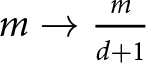 $m \to \frac{m}{d+1}$. This gives the estimate
 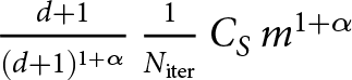 $\frac{d+1}{(d+1)^{1+\alpha}}\, \frac{1}{N_{\mathrm{iter}}}\, C_{S}\, m^{1+\alpha}$. When W-SIA is FSSA stabilized, then the decoupled solution procedure is not possible to perform anymore and the computational cost is the same as in the W-SIAStokes case, that is,
  $\frac{1}{N_{\mathrm{iter}}}\, C_{S}\, m^{1+\alpha}$.
Computing the SIA velocities by means of the closed-form expressions (9) requires 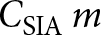 $C_{\mathrm{SIA}}\, m$ floating point operations.
The computational cost for advancing the ice surface from the initial state to time t = T is proportional to the number of time steps  $N_{\Delta t}$ we take along the way. The number of time steps itself is given by
 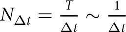 $N_{\Delta t} = \frac{T}{\Delta t} \sim \frac{1}{\Delta t}$. For a time-step restriction on the form
 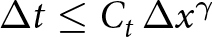 $\Delta t \leq C_t\, \Delta x^\gamma$, we have that
  $N_{\Delta t} \sim \frac{1}{\Delta x^\gamma} \sim m^{\gamma/(d-1)}$.
We now combine the computational cost estimates for obtaining the velocity functions, with the computational cost estimate for advancing the ice surface in time. The estimates for all the considered formulations are gathered in Table 1. All the parameters to evaluate the computational costs in the above table are known, except for the time-step restriction exponent γ in the case of some SIA formulations. We numerically compute the exponents γ in Section 7, and then compare the computational cost across the different formulations.
Computational cost estimates for obtaining the numerical solutions to a set of considered models. Here, m is the number of mesh vertices in the horizontal direction, d is the number of dimensions, α denotes the choice of a linear solver, γ is the time-step vs mesh size scaling exponent, CS is a constant, related to the choice of the nonlinear solver, that scales the number of nonlinear iterations used to solve the reference nonlinear Stokes problem (W-Stokes) and  $N_{\mathrm{iter}}$ is the number of iterations to solve W-Stokes
7. Numerical study
In this section, we solve SIA (9), W-SIA (18) and W-SIAStokes (19). We numerically compute the largest stable time-step size  $\Delta t$ when the free surface of an ice sheet is advected in time as described in Section 7.1. We find the dependence between
  $\Delta t$ and the horizontal mesh size
  $\Delta x$ (the Courant–Friedrich–Levy [CFL] condition), compare the errors of the different SIA solutions to the nonlinear Stokes solution and relate them to runtimes. We do this for three different geometries. The experiments are performed by using the FEniCS 2019 library (Alnaes and others, Reference Alnaes, Logg, Olgaard, Rognes and Wells2014, Alnæ s and others, Reference Alnaes2015) on a laptop with the AMD Ryzen 7 PRO 6850U processor and 16 GB RAM.
7.1. An algorithm for computing the largest feasible time step when solving the free-surface equation
In this section, we provide the criterion which we use to numerically compute the largest feasible time step  $\Delta t_*$ when updating the ice sheet surface in time using the free-surface Eqn. (1) over domain
  $\Omega^\perp$ as defined in the scope of Section 2.1. CFL condition limits
  $\Delta t_*$ in terms of the mesh size
  $\Delta x$:
 \begin{equation}
\Delta t_* = C\, \min_{x_i \in \Omega^\perp} (\Delta x)^p,\, p \gt 0,
\end{equation}
\begin{equation}
\Delta t_* = C\, \min_{x_i \in \Omega^\perp} (\Delta x)^p,\, p \gt 0,
\end{equation}where C > 0 is the CFL number depending on the type of the discretization of (1) and the data in (1), and the mesh size is:
 \begin{equation}
\Delta x = \min_{(x_i \neq x_j) \in \Omega^\perp_h} \|x_i - x_j\|_2.
\end{equation}
\begin{equation}
\Delta x = \min_{(x_i \neq x_j) \in \Omega^\perp_h} \|x_i - x_j\|_2.
\end{equation} We are interested in the exponent p from (37), where the severity of the time-step restriction increases with an increased p, whereas p = 0 implies no dependence of  $\Delta t_*$ on
  $\Delta x$. To compute
  $\Delta t_*$ numerically, we use the stability criterion:
 \begin{equation}
\int_{\Omega^\perp} (h(x,t_{k+1}))^2\, \mathrm{d}\Omega^\perp - \int_{\Omega^\perp} (h(x,t_{k}))^2\, \mathrm{d}\Omega^\perp \leq 0,\, k=1,2,3,\ldots
\end{equation}
\begin{equation}
\int_{\Omega^\perp} (h(x,t_{k+1}))^2\, \mathrm{d}\Omega^\perp - \int_{\Omega^\perp} (h(x,t_{k}))^2\, \mathrm{d}\Omega^\perp \leq 0,\, k=1,2,3,\ldots
\end{equation} which has to hold for each time  $t_k \lt T$, where
  $k=1,2,3,\ldots$. The above stability criterion measures the difference in the energy of the free-surface function across two consecutive time samples. The relation between (39) and the von Neumann analysis is the following. Within the von Neumann analysis, the surface function is written as
  $h(x,t_k) = \sum_{j=-M}^M \delta_j(t_k)\, \mathrm{e}^{i w_j x}$, where
  $w_j = \frac{2\pi\, j}{|P|}$ are wavenumbers,
  $|P|$ is the domain (interval) size and
  $\delta_j^k = \frac{1}{|P|} \int_P h(x,t_k)\, \mathrm{e}^{-i w_j x}\, \mathrm{d}x$ are the Fourier coefficients. The final statement of the von Neumann analysis is that there exists
  $\Delta t \gt 0$ such that:
 \begin{equation*}|\delta_j^{k+1}| \leq |\delta_j^{k}|.\end{equation*}
 Thus,  $\sum_{j=1}^N |\delta_j^{k+1}| \leq \sum_{j=1}^N |\delta_j^{k}|$, and using Parseval’s identity
 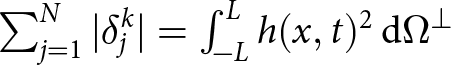 $\sum_{j=1}^N |\delta_j^{k}| = \int_{-L}^L h(x,t)^2\, \mathrm{d}\Omega^\perp$ on each side of the inequality, and then moving the right-hand-side term to the left-hand-side we obtain (39). We pose the computation of
  $\Delta t_*$ as the following optimization problem. Find
  $\max \Delta t_*$ subject to:
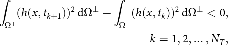 \begin{equation}
\begin{aligned}
\int_{\Omega^\perp} (h(x,t_{k+1}))^2\, \mathrm{d}\Omega^\perp - \int_{\Omega^\perp} (h(x,t_k))^2\, \mathrm{d}\Omega^\perp \lt 0,\\
k=1,2,\ldots,N_T,
\end{aligned}
\end{equation}
\begin{equation}
\begin{aligned}
\int_{\Omega^\perp} (h(x,t_{k+1}))^2\, \mathrm{d}\Omega^\perp - \int_{\Omega^\perp} (h(x,t_k))^2\, \mathrm{d}\Omega^\perp \lt 0,\\
k=1,2,\ldots,N_T,
\end{aligned}
\end{equation} where  $\int_{\Omega^\perp} (h(x,t_{k+1}))^2\, \mathrm{d}\Omega^\perp$ and
  $\int_{\Omega^\perp} (h(x,t_k))^2\, \mathrm{d}\Omega^\perp$ are the free-surface energies evaluated in two consecutive time steps, and NT is the number of time steps to perform the simulations in time
  $t \in (0, T]$. The stability criterion (40) applies to simulations where the physical (exact) surface energy does not grow in time.
To understand how  $\Delta t_*$ depends on
  $\Delta x$, we discretize (1) using different mesh sizes
  $(\Delta x)_j$,
  $j=1,2,\ldots$, and then for each
  $(\Delta x)_j$ compute
  $(\Delta t_*)_j$ by solving one optimization problem (40). We solve the optimization problem using the bisection method. Once all the data pairs
  $((\Delta x_*)_j, \Delta t_*)_j)$,
  $j=1,2,\ldots$, are known, we approximate the exponent p in (37) by fitting a linear function to the transformed data pairs
  $((\log_{10} \Delta x_*)_j, (\log_{10} \Delta t_*)_j)$,
  $j=1,2,\ldots$, where p takes the value of the slope of the fitted linear function. Note that this is a fairly computationally expensive procedure, which is the reason why we restrict ourselves to two dimensions in this study.
7.2. Slab on a slope with perturbed surface
7.2.1. Configuration
First, we run experiments for a slab on a slope with a perturbed surface, as this is the setting of the von Neumann analysis in (A). The ice sheet is a 2-D slab,  $L=80{\times} 10^3\,\mathrm{{m}}$ long and
  $H=1 {\times} 10^3\,\mathrm{{m}}$ thick, inclined with
  $\alpha=0.75^{\circ}$ measured in the clockwise direction, with the initial surface:
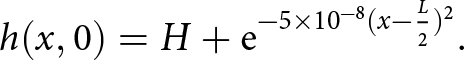 \begin{equation*}h(x,0) = H + \mathrm{e}^{-5 {\times} 10^{-8} (x - \frac{L}{2})^2}.\end{equation*}
 For the free-surface Eqn. (1), we impose periodic boundary conditions (2) as this is required for the von Neumann analysis. We impose no-slip boundary conditions on  $\Gamma_b$, stress-free boundary conditions on
  $\Gamma_s$ and periodic boundary conditions on
  $\Gamma_l$.
The relation between the number of discretization points in the horizontal direction  $n_x=m$ and
  $\Delta x$ that we use to perform the experiments is given in Table 2. Note that
 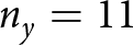 $n_y=11$ (corresponding to
 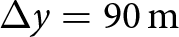 $\Delta y = 90\,\mathrm{{m}}$) is fixed for all experiments and the FSSA scaling parameter is fixed at θ = 1, unless stated otherwise.
Number of the discretization points in the horizontal direction nx and the corresponding horizontal mesh size  $\Delta x$ for the slab on a slope surface case
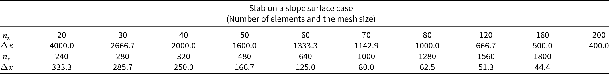
7.2.2. Accuracy
In Fig. 2, we show how the perturbed surface evolves in time, where the final simulation time is t = 100 years. Here the solution is computed using the nonlinear Stokes problem which we consider a reference, with a small time step  $\Delta t=0.1$ years, the horizontal mesh size
  $\Delta x=250\,\mathrm{{m}}$ and the vertical mesh size
  $\Delta y = 90\,\mathrm{{m}}$. In Fig. 3, we plot the solutions of the different SIA problem formulations to the reference solution, where all the solutions are evaluated at t = 6 years. We observe that all the solutions are close to the reference solution. The solution to W-SIAStokes appears overall closest to the reference. The addition of the FSSA stabilization term increases the error, but not significantly.
Propagation of the surface elevation function in time when computed as a solution to the nonlinear Stokes problem (reference), where the simulation time step is  $\Delta t = 0.1$ years. Horizontal mesh size and vertical mesh size are
  $\Delta x = 250\,\mathrm{{m}}$ and
  $\Delta y = 90\,\mathrm{{m}}$, respectively.
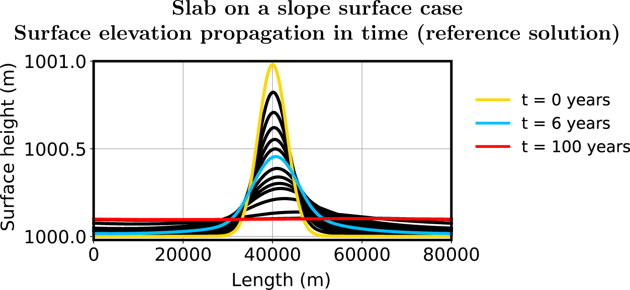
Surface elevations at simulation time t = 6 years for different SIA problem formulations and the reference formulation (nonlinear Stokes problem). Horizontal and vertical mesh sizes are  $\Delta x = 250\,\mathrm{{m}}$ and
  $\Delta y = 90\,\mathrm{{m}}$, respectively. The largest feasible time step
  $\Delta t_*$ for the given
  $\Delta x$ and
  $\Delta y$ is chosen for each formulation:
  $\Delta t_* = 6$ years,
  $\Delta t_* = 12$ years,
  $\Delta t_* = 1.8$ years,
  $\Delta t_* = 0.04$ years,
  $\Delta t_* = 0.008$ years,
  $\Delta t = 0.1$ years for W-SIAStokes-FSSA, W-SIA-FSSA, W-SIAStokes, W-SIA, SIA, Reference, respectively.
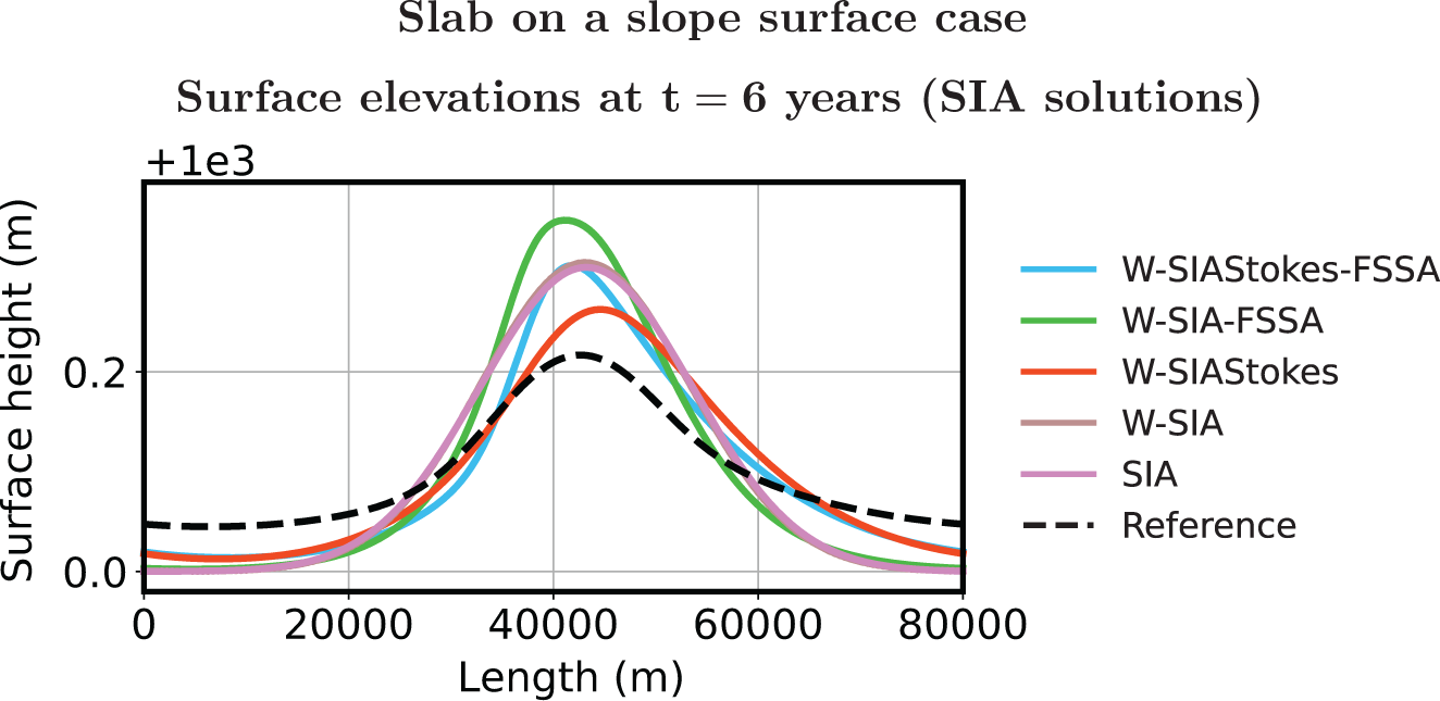
7.2.3. Time-step restriction scaling
Now we compute  $\Delta t_*$ as a function of
  $\Delta x$ as described in Section 7.1. We run the simulations with and without the FSSA terms defined in the scope of Section 5. The final simulation times are adjusted to the magnitude of the largest time-step sizes making the comparison more realistic. We use the final simulation times: t = 100 years (W-SIAStokes-FSSA and W-SIA-FSSA), t = 12 years (W-SIAStokes and W-SIA) and t = 5 years (SIA). The results are shown in the first plot of Fig. 4. We observe that the largest stable time step
  $\Delta t_*$ is allowed to be from 10 times (coarse resolution) to 100 times (fine resolution) larger when using W-SIAStokes as compared to W-SIA. Furthermore, in W-SIAStokes,
  $\Delta t_*$ has a constant relation to
  $\Delta x$ over the whole range of the chosen
  $\Delta x$ except for the finest resolution where the relation becomes linear. The allowed time steps when using SIA and W-SIAStokes are small. The
  $\Delta_* t$ vs
  $\Delta x$ scaling in the latter two formulations is quadratic which is less desired.
(a) Scaling of the largest feasible time step  $\Delta t_*$ as a function of the horizontal mesh size
  $\Delta x$ when the vertical mesh size
  $\Delta y = 90\,\mathrm{{m}}$ is fixed. (b) The model error as a function of the wall clock runtime when the nonlinear Stokes solution is taken as a reference. In all cases, the final time is fixed at t = 20 years. Mesh sizes
  $\Delta x = 250\,\mathrm{{m}}$ and
  $\Delta y = 90\,\mathrm{{m}}$ are also fixed. The time step is refined starting at the formulation largest feasible time step
  $\Delta t = \Delta t_*, \Delta t_*/2, \Delta t_*/4,\ldots.$ The time step for the reference solution is fixed at
  $\Delta t = 0.1$ years.
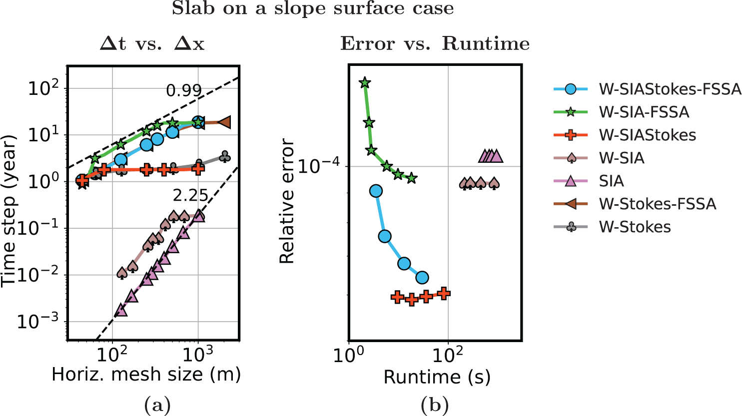
7.2.4. Run-time versus accuracy
Next, we perform an experiment measuring the ratio between the relative model error and the computational (wall clock) runtime for each of the SIA formulations. This is important as a small  $\Delta t$ does not necessarily imply a small computational time for the whole simulation. This depends on the computational time required to evaluate the velocity functions in each time step. We set the final simulation time to t = 20 years. For W-SIAStokes-FSSA, we used
  $\Delta t = 6, 3, 1.5, 0.75$. For W-SIA-FSSA, we used
  $\Delta t = 12, 6, 3, 1.5, 0.75, 0.4$. For W-SIAStokes, we used
  $\Delta t = 1.8, 0.9, 0.45, 0.2$. For W-SIA, we used
  $\Delta t = 0.04, 0.03, 0.02, 0.01$, and for SIA we used
  $\Delta t = 0.008, 0.007, 0.006, 0.005$. The error is computed with the nonlinear Stokes solution as a reference with
  $\Delta t = 0.1$ years. In all cases, the mesh sizes
  $\Delta x = 250\,\mathrm{{m}}$ and
  $\Delta y = 90\,\mathrm{{m}}$ are fixed. The result is given in the second plot of Fig. 4. We observe that W-SIAStokes-FSSA allows small computational runtimes with only a mild increase in the model error. W-SIA-FSSA also allows for small computational runtimes, but the model error is larger than in the W-SIAStokes-FSSA case. The unstabilized (weak nor strong) SIA formulations do not allow for small computational runtimes, except in the case when we use the W-SIAStokes formulation.
7.2.5. Impact of the FSSA parameter θ on the time-step restriction scaling
As we demonstrated in the previous paragraphs, W-SIAStokes-FSSA allows for the largest time steps among all the considered formulations. The FSSA parameter in those experiments was fixed at θ = 1. In Fig. 5, we illustrate the effect of the choice of θ on the scaling of the largest feasible time step  $\Delta t_*$ as a function of
  $\Delta x$. We observe that choice of small θ leads to a non-robust
  $\Delta t_*$ vs
  $\Delta x$ scaling behaviour, where
  $\Delta t_*$ has to be taken around 10 times smaller as θ → 0. As the FSSA parameter approaches θ = 0.2 then the
  $\Delta t_*$ vs
  $\Delta x$ scaling approaches the linear behaviour as also observed in Fig. 4. Furthermore, the scaling stays the same for θ > 0.2. This implies that, for the given test case, the choice of θ is not sensitive and can be left at θ = 1 without losing the length of the largest feasible time step.
Largest feasible time step  $\Delta t_*$ as a function of the horizontal mesh size
  $\Delta x$ for the W-SIAStokes-FSSA formulation, when the FSSA parameter θ varies. Vertical mesh size is fixed at
  $\Delta y = 83.3\,\mathrm{{m}}$ in (a) and at
  $\Delta y = 41.67\,\mathrm{{m}}$ in (b).
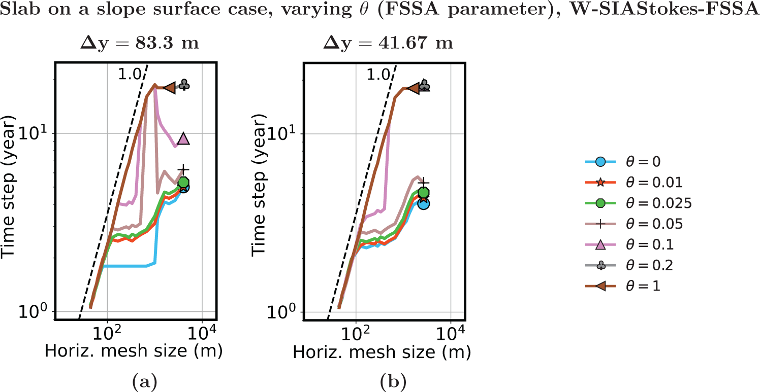
7.3. An idealized ice sheet surface case
7.3.1. Configuration
We now change the configuration to study the impact of ice sheet margins. The ice sheet configuration in this test case takes horizontal values  $x \in [-L, L]$ and vertical values
  $y \in [0, H]$, where the ice sheet half half-length is
  $L = 750 {\times} 10^{3}\,\mathrm{{m}}$ and the ice sheet height is
  $H = 3 {\times} 10^{3}\,\mathrm{{m}}$. To construct the ice sheet surface for this test case, we define the following auxiliary profile:
 \begin{equation*}h_1(x) = \left(3 - \left(\frac{x}{L}\right)^2 \right)^{0.58},\end{equation*}
and then use it in the initial surface definition:
 \begin{equation*}h (x,0) = H\, \frac{h_1(x) - h_1(-L)}{h_1(0)}.\end{equation*}
 When solving the free-surface Eqn. (1), we set Dirichlet boundary conditions  $h(-L,t) = h(-L,0)$ on the left boundary and
  $h(L,t) = h(L,0)$ on the right boundary. When solving one of the momentum balances, we impose no-slip boundary conditions on
  $\Gamma_b$ and
  $\Gamma_l$, whereas on
  $\Gamma_s$ we set stress-free boundary conditions.
The relation between the number of horizontal mesh elements nx and horizontal mesh size  $\Delta x$ that we use to perform the experiments is given in Table 3.
Number of the discretization points in the horizontal direction nx and the corresponding horizontal mesh size  $\Delta x$ for the idealized ice sheet surface case.
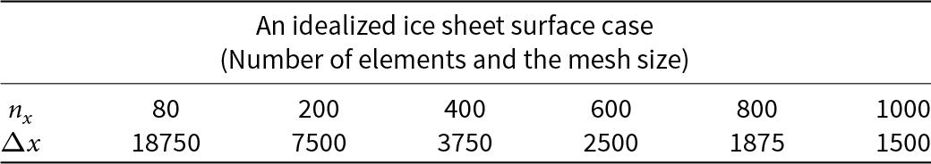
Note that the number of vertical mesh elements is  $n_y=12$ (corresponding to vertical mesh size
  $\Delta y = 250\,\mathrm{{m}}$) and is fixed for all experiments unless stated otherwise. The FSSA scaling parameter is always fixed at θ = 1.
7.3.2. Time-step restriction scaling
In the left plot of Fig. 6, we display the largest feasible time step  $\Delta t_*$ as a function of
  $\Delta x$ for the different SIA formulations. Time step
  $\Delta t_*$ scales linearly with respect to
  $\Delta x$ for W-SIAStokes and W-SIAStokes-FSSA. For SIA and W-SIA, we observe a quadratic scaling. The benefits when using the FSSA stabilization terms together with W-SIA disappear as the
  $\Delta x$ is fine enough. Among all the formulations, the largest time steps can be taken when W-SIAStokes W-SIAStokes-FSSA are used. For W-SIAStokes-FSSA, the time steps increase approximately 100 times, across the whole range of the considered mesh sizes. In the W-SIAStokes case, the addition of the FSSA stabilization terms allows for a significantly smaller computational time but gives rise to a (typically small) increase in the approximation error.
(a) Scaling of the largest feasible time step  $\Delta t_*$ as a function of the horizontal mesh size
  $\Delta x$ when the vertical mesh size
  $\Delta y = 90\,\mathrm{{m}}$ is fixed. (b) The model error as a function of the wall clock runtime when the nonlinear Stokes solution is taken as a reference. In all cases, the final time is fixed at t = 20 years. Mesh sizes
  $\Delta x = 250\,\mathrm{{m}}$ and
  $\Delta y = 90\,\mathrm{{m}}$ are also fixed.
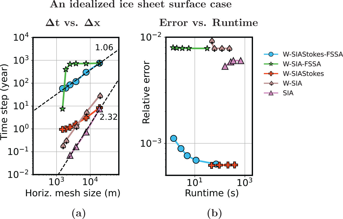
7.3.3. Run-time versus accuracy
In the next experiment, we compute the ratio between the computational runtime (wall clock) and the modelling error. For all formulations, we fixed the horizontal mesh size to  $\Delta x = 3750\,\mathrm{{m}}$ and ran the simulation until t = 100 years. The error is computed using the nonlinear Stokes solution as a reference, where the time step is
  $\Delta t = 0.1$ years. The maximum time steps for testing each SIA formulation is taken in line with the largest feasible time step for
  $\Delta x = 3750\,\mathrm{{m}}$ from Fig. 6. For both FSSA stabilized weak SIA formulations, we used
  $\Delta t = 50, 25, 12.5, 6, 1$. For W-SIAStokes, we used
  $\Delta t = 1.6, 0.8, 0.4, 0.2$. For W-SIA, we used
  $\Delta t = 1, 0.8, 0.4, 0.2$ and for SIA we used
  $\Delta t = 0.16, 0.1, 0.08, 0.04$. The results are presented in Fig. 6, plot on the right. Runtime vs error ratio of W-SIASTokes is favourable over all the other formulations that we consider. This is, both, when the FSSA terms are present, and when the FSSA terms are not present.
7.3.4. Long time simulations
We now compute the surface evolution over a long period: the final time is  $t=10^4$ years. We choose a fine mesh size
  $\Delta x = 1500\,\mathrm{{m}}$. The time step is chosen in line with Fig. 6 (left plot) for the given
  $\Delta x$, that is,
  $\Delta t = 58.2$ years for W-SIAStokes and
  $\Delta t = 7.5$ years for W-SIA. In Fig. 7, we show the solutions obtained from the two formulations. The solution obtained using W-SIAStokes does not entail any oscillations, whereas the solution in the W-SIA case entails oscillations close to the lateral boundaries. We have not fully explored the behaviour. However, we speculate that this is due to the lack of control over all strain components in W-SIA (see (18)) in contrast with W-SIAStokes (19), where all the strain components are present. This implies that a bound
 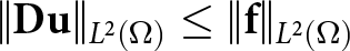 $\|\mathbf{D} \mathbf{u}\|_{L^2(\Omega)} \leq \| \mathbf{f}\|_{L^2(\Omega)}$, where
  $\mathbf{f}$ is the gravity field, can be obtained by using Korn’s inequality. This provides control over the derivatives of the velocities
  $\mathbf{u}$, which prevents
  $\mathbf{u}$ from being too oscillatory.
Two surface evolutions after  $t=10^4$ years. The horizontal mesh size is
  $\Delta x = 1500\,\mathrm{{m}}$, whereas the vertical mesh size is
  $\Delta y = 250\,\mathrm{{m}}$. The time steps take the largest feasible values for the given mesh sizes:
 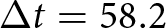 $\Delta t = 58.2$ years for W-SIAStokes in (a) and
  $\Delta t = 7.5$ years for W-SIA in (b). Both formulations are stabilized using the FSSA stabilization terms with the FSSA parameter set to θ = 1.
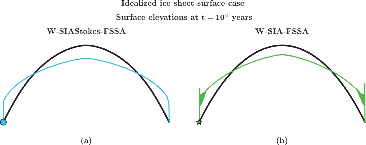
7.4. A 2-D cross section of Greenland
7.4.1. Configuration
In this test case, we still consider a 2-D ice sheet geometry, but with a more realistic initial surface elevation as well as a more realistic bedrock elevation. We simplify the full three-dimensional (3-D) Greenland geometry obtained from BedMachine Morlighem and others Reference Morlighem(2017) and intersect it with a horizontal line to get the boundary points over a cross section as displayed in Fig. 8. Then we represent the surface elevation and the bedrock elevation by using a cubic spline interpolation. This allows for evaluating the surfaces at an arbitrary location, which we employ when considering horizontally varying mesh sizes in our computational study.
Top view over the Greenland geometry (Morlighem and others, Reference Morlighem2017) (a), where the intersecting red line gives the boundary of the Greenland cross section (b) used as one of the computational domains in this paper.
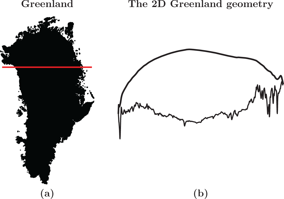
When solving the free-surface Eqn. (1), we set Dirichlet boundary conditions  $h(-L,t) = h(-L,0)$ on the left boundary and
  $h(L,t) = h(L,0)$ on the right boundary. When solving one of the momentum balances, we impose no-slip boundary conditions on
  $\Gamma_b$ and
  $\Gamma_l$, whereas on
  $\Gamma_s$ we set stress-free boundary conditions.
The relation between the number of horizontal mesh elements nx and horizontal mesh size  $\Delta x$ that we use to perform the experiments is given in Table 4.
Number of the discretization points in the horizontal direction nx and the corresponding horizontal mesh size  $\Delta x$ for the Greenland (2-D) profile case
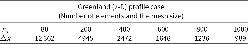
7.4.2. Time-step restriction scaling
In Fig. 9 (left plot), we investigate the scaling of  $\Delta t$ as a function of
  $\Delta x$. We observe that in the case of W-SIAStokes, the order of scaling is
  $\sim$$0.75$, whereas in the W-SIAStokes-FSSA case, the order of scaling is close to 0.5. The scaling in the W-SIA case is approximately of order 2, which is similar as in all previous test cases. When W-SIA-FSSA is used the scaling behaves unpredictably, similar as in Section 7.3. Among all the formulations, the time steps are the largest in the W-SIAStokes-FSSA.
(a) Scaling of the largest feasible time step  $\Delta t_*$ as a function of the horizontal mesh size
  $\Delta x$ when the vertical mesh size is fixed. (b) The model error as a function of the wall clock runtime when the nonlinear Stokes solution is taken as a reference. In all cases, the final time is fixed at t = 400 years. The horizontal mesh size is fixed at
  $\Delta x=2472\,\mathrm{{m}}$.
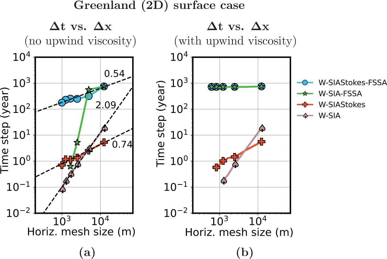
7.4.3. Upwinding
After visualizing the computed solutions using all the considered SIA formulations, we observed spurious oscillations over the western part of the 2-D Greenland geometry (see Fig. 10). For that reason, we in addition combined the SIA formulations with the first-order viscosity (also upwind viscosity) operator added to the free-surface equation. The role of that operator is dampening of the spurious oscillations. In Fig. 9 (right plot), we compute the scaling of  $\Delta t$ as a function of
  $\Delta x$ when the first-order viscosity operator is added to the free-surface equation, for each of the considered SIA formulations. We observe that the scaling does not change when no FSSA terms are added W-SIAStokes or W-SIA. However, the scaling, when the FSSA terms are employed, changes from linear (no first-order viscosity) to constant (with first-order viscosity). The latter is favourable.
Surface evolutions computed using different SIA formulations, after t = 400 years. The horizontal mesh size is  $\Delta x = 2472\,\mathrm{{m}}$. The time steps take the largest feasible values for the given mesh sizes (see Figure 9).
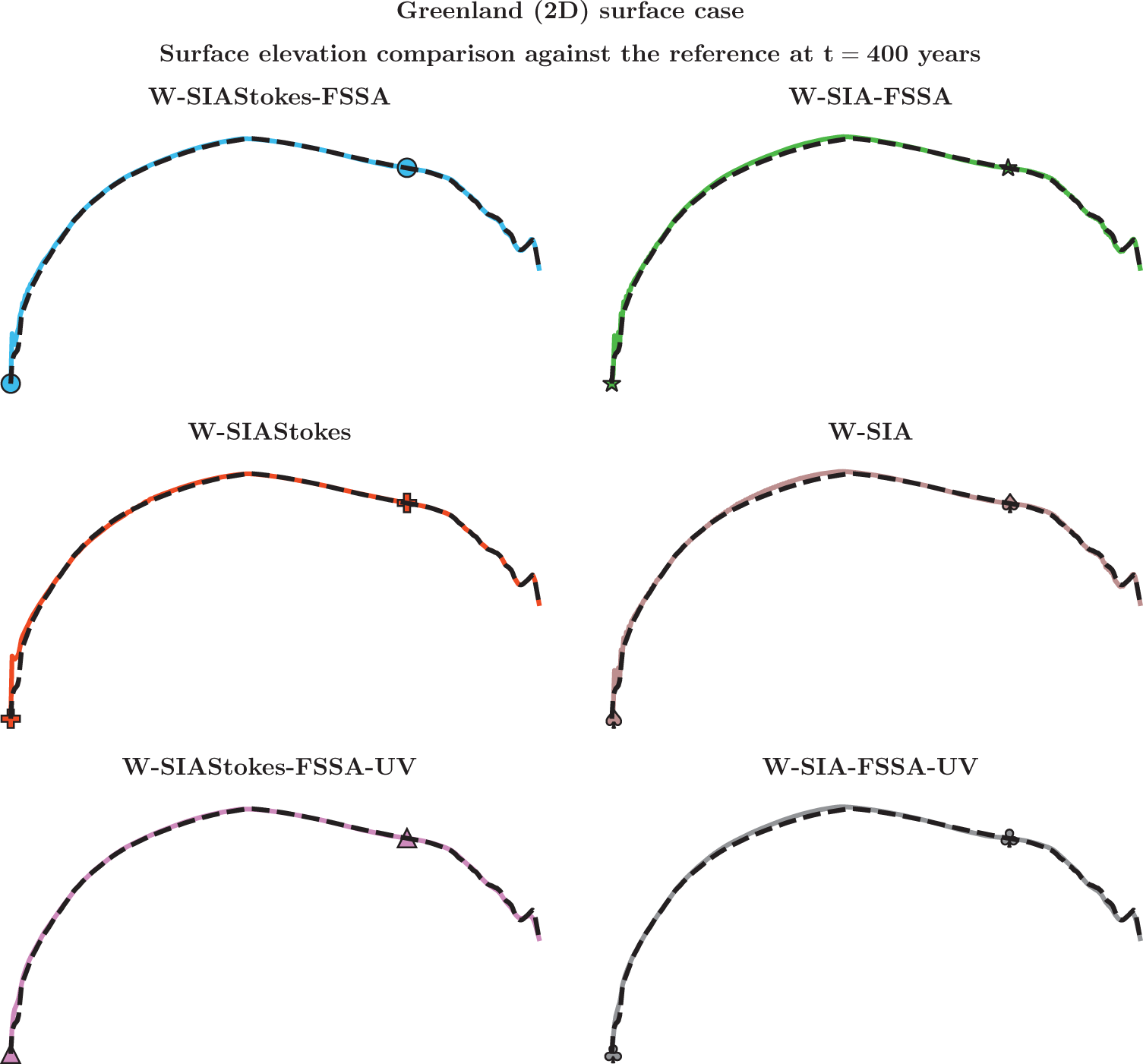
7.4.4. Long time simulations
In Fig. 10, we, for each of the considered SIA formulations, plot the surface elevations after t = 400 years of simulation time, at  $\Delta x = 2472\,\mathrm{{m}}$, and make a comparison towards the surface elevations computed using the nonlinear Stokes problem (reference). We observe that all the SIA formulation solutions are overall a good approximation to the reference solution. As stated in the previous paragraph, the solutions in cases W-SIAStokes-FSSA, W-SIA-FSSA, W-SIAStokes, and W-SIA, displayed in Fig. 10 involve spurious oscillation at the western part of the 2-D Greenland geometry. The plots in the last row of Fig. 10 display the viscous solutions, that is, W-SIAStokes-FSSA-UV and W-SIA-FSSA-UV, a where we observe that the oscillations have disappeared. The oscillations in the W-SIAStokes-FSSA-UV and W-SIA-FSSA-UV cases were also removed at $t=10000$ years, as
  $t=10\,000$ in Fig. 12
7.4.5. Run-time versus accuracy
In Fig. 11, compute the ratio between the computational runtime (wall clock) and the modelling error. For all formulations, we fixed the horizontal mesh size to  $\Delta x = 2472$ m and ran the simulation until t = 400 years. The error is computed using the nonlinear Stokes solution as a reference, where the time step is
  $\Delta t = 0.4$ years. The maximum time steps for testing each SIA formulation is taken in line with the largest feasible time step for
  $\Delta x = 2472\,\mathrm{{m}}$ from Fig. 9. For W-SIAStokes-FSSA, we used
  $\Delta t = 249, 125, 60, 30, 10, 1, 0.5$ years. For W-SIA-FSSA, we used
  $\Delta t = 5, 2.5, 1, 0.5, 0.4$ years. For W-SIAStokes, we used
  $\Delta t = 1.37, 0.9, 0.65, 0.4$ years. For W-SIA, we used
  $\Delta t = 0.76, 0.6, 0.5, 0.4$. When W-SIAStokes-FSSA and W-SIA-FSSA are further augmented with the with upwind viscosity in the free-surface equation, we used
  $\Delta t = 800, 400, 200, 100, 50, 25, 12.5$ years. We observe that the FSSA stabilized weak formulations augmented with the upwind viscosity term have by far the best error vs runtime ratio.
Approximate model error as a function of the wall clock runtime when the nonlinear Stokes solution is taken as a reference. In all cases, the final time is fixed at t = 400 years. The horizontal mesh size is  $\Delta x = 2472$.
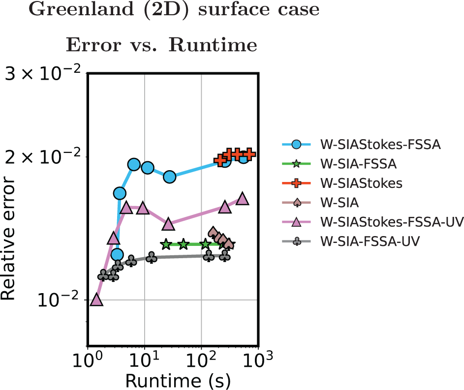
Surface elevations computed using the FSSA stabilized SIA formulations, with and without the first-order (upwind) viscosity added to the free-surface equation. The surface elevations are evaluated at  $t=10\,000$ years. The horizontal mesh size is
  $\Delta x = 2472\,\mathrm{{m}}$. The time steps take the largest feasible values for the given mesh sizes (see Figure 9).
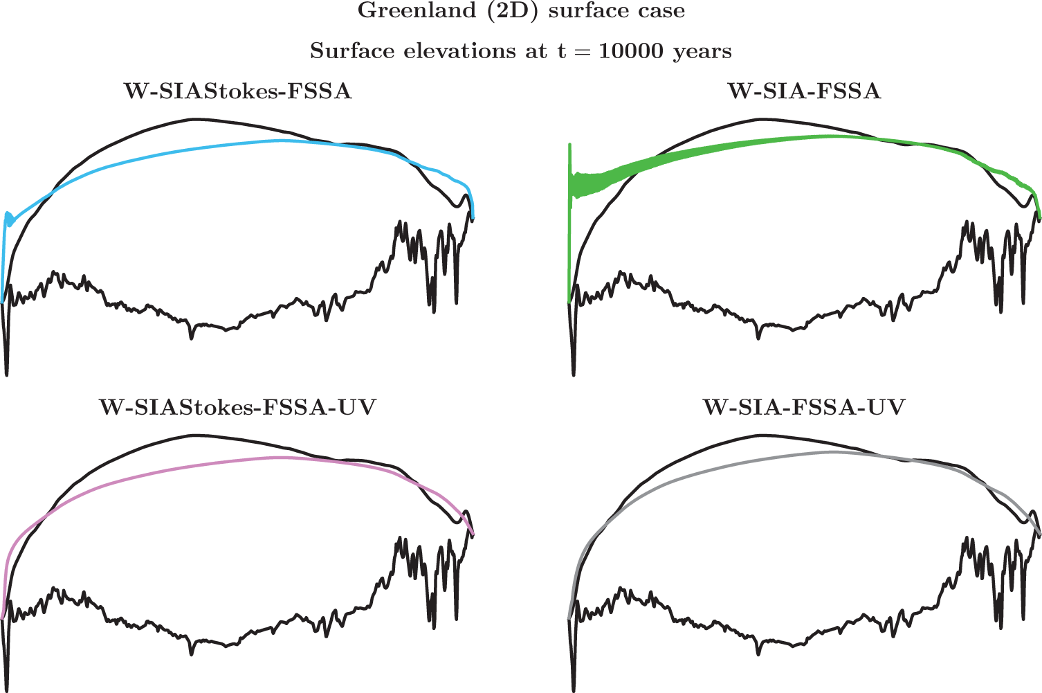
7.5. Computational cost estimates with the parameters inferred from the numerical experiments
In the subsections above, we gathered experimental data on the slope of the scaling of the time-step restriction as a function of the horizontal mesh size. In this subsection, we use those slopes in place of the parameter γ in Section 6, to speculate on the relation between computational work and the number of horizontal mesh nodes m for the different momentum models. Across the experiments, we observe that W-SIA-FSSA, W-SIAStokes and W-SIAStokes-FSSA have a linear time-step constraint γ = 1. On Greenland with upwind viscosity, we saw that γ can also be smaller than 1, but we here chose the worst-case scenario value (γ = 1) for W-SIA-FSSA and W-SIAStokes. In the W-SIA model case, the worst case is γ = 2. The same holds for the standard SIA model case. We gather these results in Table 5. In the W-Stokes-FSSA case, we get γ = 1, whereas in the W-Stokes case, we have γ = 1 when the horizontal mesh size is small and γ = 0 for larger horizontal mesh sizes—the worst case is then γ = 1.
Computational cost estimate comparison across the different formulations of the shallow ice approximation (SIA) model, when using the solution (the velocity) to advance the ice sheet surface in time. Here, m is the number of mesh vertices in the horizontal direction, d is the number of dimensions, α denotes the choice of a linear solver, γ is the time-step vs mesh size scaling exponent, CS is a constant, related to the choice of the nonlinear solver, that scales the number of nonlinear iterations used to solve the reference nonlinear Stokes problem (W-Stokes) and  $N_{\mathrm{iter}}$ is the number of iterations to solve W-Stokes
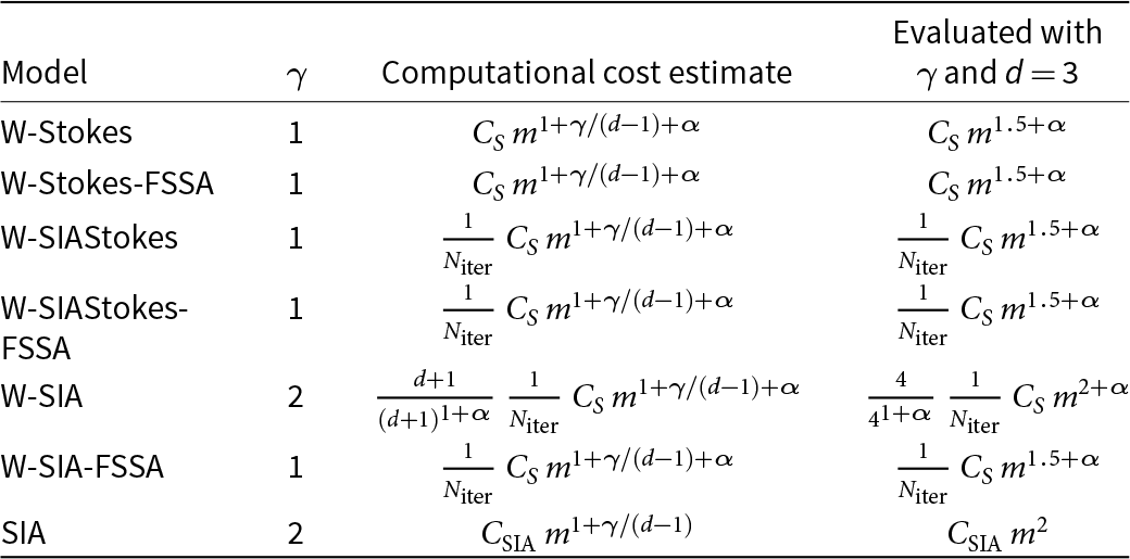
We observe that the SIA model has the lowest asymptotic cost scaling m 2. The next best is W-SIAStokes-FSSA with m 2.5 when α = 1 (sparse direct solver). We argue that the computational cost is in the two cases comparable when it comes to the asymptotic scaling as  $m\to\infty$. However, knowing that the SIA model is a crude simplification of the Stokes model (4), and that the W-SIAStokes model only carries minor simplified elements (the viscosity) as compared to W-Stokes, the W-SIAStokes model is more accurate as we could also observe from the runtime vs error experiments figures. The computational cost in the W-SIA model also scales as
  $m^{1.5+\alpha}$, but this does not hold for all the horizontal mesh size choices as observed from the experiments. We note that
  $N_\mathrm{nlin}$ is large for large
  $\Delta t$. This is due to that the nonlinear iteration initial guess to compute the solution at time
  $t_{k+1}$ is the solution from time tk, and the two solutions when
  $\Delta t = t_{k+1} - t_k$ is large are typically very different, implying that the nonlinear iteration count is large.
The time-step sizes can also be restricted by some other components of an ice sheet model, such as the temperature evolution or climate data. However, when these time-step sizes are small, it is still not certain that the velocity solution has to be updated at the same small time step as, e.g., the temperature. This study is out of the scope of this paper.
8. Final remarks
In this paper, we investigated the benefits when using the SIA momentum balance model (A1) written on different weak formulations. We referred to the weak SIA model (18) as W-SIA, the modified weak SIA model alias weak form linear Stokes equations employing the SIA viscosity function as W-SIAStokes, the weak full nonlinear Stokes problem as W-SIA and to the standard (strong form) SIA model as SIA. When the different SIA forms were additionally stabilized by mean of the FSSA terms (23), we appended an abbreviation FSSA to each of the form abbreviations.
The key outcomes of the present study are that in the considered test cases:
• W-SIA-FSSA allows for large time steps with linear scaling, but limited to coarse
$\Delta x$.• W-SIAStokes and W-SIAStokes-FSSA have linear time-step restriction scaling for all
$\Delta x$.• W-SIAStokes is numerically more robust and accurate compared to W-SIA for a small cost increase.


We expand on the list above in the paragraphs written below.
The first weak formulation is W-SIA (18). An immediate benefit when using W-SIA is that we were able to add the FSSA stabilization terms (23) (W-SIA-FSSA). This improved the time-step restriction from quadratic (W-SIA) to linear (W-SIA-FSSA) scaling in terms of the horizontal mesh size  $\Delta x$ when using the W-SIA velocities for solving the free-surface equation. Overall, the time-step sizes in all the considered test cases were increased by at least approximately 100 times as compared to the standard SIA formulation time-step sizes. However, we observed that when
  $\Delta x$ is small enough, the largest time-step size behaviour became unpredictable and started taking values similar to the standard SIA time-step sizes. We have not experimentally assessed the largest feasible time steps in 3-D. However, according to our computational cost estimates, the differences across SIA and W-SIA-FSSA are smaller in 3-D.
As a remedy, we modified W-SIA to W-SIAStokes (19) by adding the originally neglected stress terms back to W-SIA but kept the SIA viscosity (13) intact so that W-SIAStokes remained a linear problem. We observed predictable largest time-step size behaviour. The time step scaled linearly in terms of  $\Delta x$ without even adding the FSSA stabilization terms to the weak formulation. After we added the FSSA stabilization terms to W-SIAStokes (W-SIAStokes-FSSA), the scaling remained linear, but the largest time-step sizes have in general significantly increased, whereas the approximation error increased only slightly. In one of the tests we compared W-SIAStokes to W-Stokes and found that the time-step sizes, including the scaling in terms of
  $\Delta x$, were comparable.
When compared to the standard SIA model, W-SIA and W-SIAStokes models had a smaller error, taking the W-Stokes solution as a reference. This held also when the FSSA stabilization terms were added to the two weak formulations and very long time steps were used. The error vs runtime ratio was also favourable in the case of both weak formulations (with and without the FSSA stabilization) over the standard SIA solution. Among the two, W-SIAStokes had a better error vs runtime ratio (with and without the FSSA stabilization). We note that the runtime measurements could differ depending on the code implementation of the different SIA formulations.
To view the observed runtime measurements from another angle, we performed a theoretical computational cost estimation in Section 6. Based on that, we conclude that the computational cost of W-SIA and W-SIAStokes is comparable to that of the standard SIA model, in terms of the asymptotic behaviour, that is, when the number of the horizontal mesh vertices is increased.
Throughout the paper, we used no-slip boundary conditions for simplicity. The FSSA stabilization terms are effective also when using the moderate slip boundary conditions (Löfgren and others, Reference Lofgren, Zwinger, Raback, Helanow and Ahlkrona2023).
We anticipate that glaciologists interested in the ice spin-up simulations of which the simulation length is on the order of hundreds of thousands of years could benefit from using the W-SIA-FSSA model or the W-SIAStokes-FSSA model over the standard SIA model. Note that our results are for isothermal simulations. More studies are needed to investigate the time-step restrictions related to temperature evolution and other physical processes. However, we believe resolving the restriction due to the velocity-surface coupling is the most difficult problem.
We speculate that the W-SIAStokes model is a good choice to replace the standard SIA model within the scope of coupled models. One of them is the ISCAL (Ice Sheet Coupled Approximation Level) model (Ahlkrona and others, Reference Ahlkrona, Lötstedt, Kirchner and Zwinger2016) where the standard SIA model and the W-Stokes model are used dynamically over an ice sheet geometry, depending on the desired modelling accuracy. When both models are coupled together, the time-step restriction is bound to that of the SIA model (quadratic scaling in terms of  $\Delta x$), whereas the W-SIAStokes model allows for linear scaling.
Acknowledgements
We thank André Löfgren from Stockholm University for valuable discussions on FSSA. We thank Christian Helanow for providing parts of the code used to perform the numerical experiments. Josefin Ahlkrona and Igor Tominec were funded by the Swedish Research Council, grant number 2021-04001. Josefin Ahlkrona also received funding from Swedish e-Science Research Centre (SeRC).
Appendix A. Von Neumann stability analysis
A.1. Without FSSA
A.1.1. Coupling
The solution to the strong form SIA
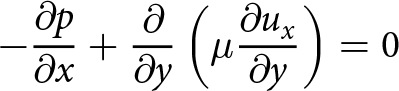 \begin{equation}
- \frac{\partial p}{\partial x}+\frac{\partial }{\partial y}\left(\mu\frac{\partial u_x}{\partial y}\right)=0
\end{equation}
\begin{equation}
- \frac{\partial p}{\partial x}+\frac{\partial }{\partial y}\left(\mu\frac{\partial u_x}{\partial y}\right)=0
\end{equation}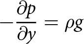 \begin{equation}
-\frac{\partial p}{\partial y} = \rho g
\end{equation}
\begin{equation}
-\frac{\partial p}{\partial y} = \rho g
\end{equation}is in the isothermal case
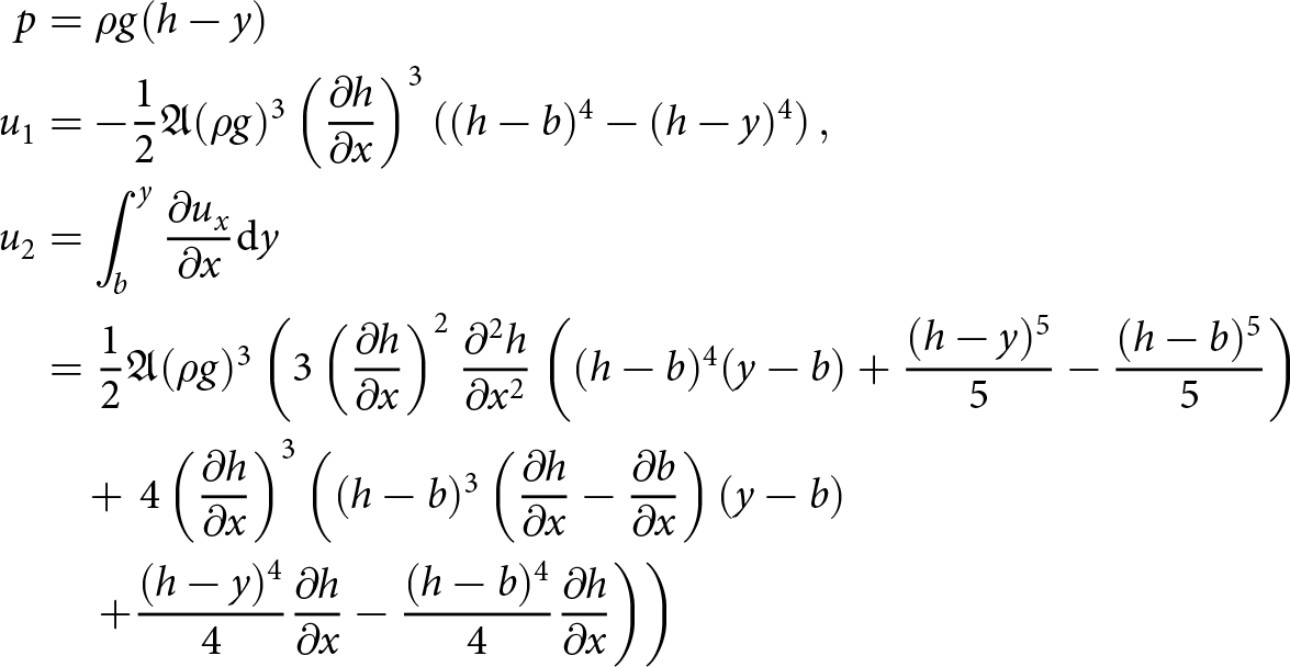 \begin{align*}
p &=\rho g (h-y)\\
u_1 &= - \frac{1}{2}\mathfrak{A} (\rho g)^3 \left(\frac{\partial h}{\partial x}\right)^3 \left( (h-b)^4- (h-y)^4 \right),\\
u_2&=\int_b^y \frac{\partial u_x}{\partial x} \mathrm{d}y \\
&= \frac{1}{2}\mathfrak{A} (\rho g)^3\left(3 \left( \frac{\partial h}{\partial x} \right)^2 \frac{\partial^2 h}{\partial x^2} \left( (h-b)^4 (y-b)+\frac{(h-y)^5}{5}-\frac{(h-b)^5}{5}\right) \right. \\
& \quad + \left.4 \left( \frac{\partial h}{\partial x} \right)^3 \left((h-b)^3\left( \frac{\partial h}{\partial x}-\frac{\partial b}{\partial x} \right) (y-b) \right.\right.\\
&\quad \left.\left.+ \frac{(h-y)^4}{4}\frac{\partial h}{\partial x}-\frac{(h-b)^4}{4}\frac{\partial h}{\partial x}\right)\right)
\end{align*}
\begin{align*}
p &=\rho g (h-y)\\
u_1 &= - \frac{1}{2}\mathfrak{A} (\rho g)^3 \left(\frac{\partial h}{\partial x}\right)^3 \left( (h-b)^4- (h-y)^4 \right),\\
u_2&=\int_b^y \frac{\partial u_x}{\partial x} \mathrm{d}y \\
&= \frac{1}{2}\mathfrak{A} (\rho g)^3\left(3 \left( \frac{\partial h}{\partial x} \right)^2 \frac{\partial^2 h}{\partial x^2} \left( (h-b)^4 (y-b)+\frac{(h-y)^5}{5}-\frac{(h-b)^5}{5}\right) \right. \\
& \quad + \left.4 \left( \frac{\partial h}{\partial x} \right)^3 \left((h-b)^3\left( \frac{\partial h}{\partial x}-\frac{\partial b}{\partial x} \right) (y-b) \right.\right.\\
&\quad \left.\left.+ \frac{(h-y)^4}{4}\frac{\partial h}{\partial x}-\frac{(h-b)^4}{4}\frac{\partial h}{\partial x}\right)\right)
\end{align*} defining  $H=(h-b)$ and considering only the surface y = h we get:
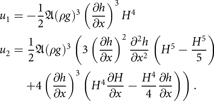 \begin{align*}
u_1 &=- \frac{1}{2}\mathfrak{A} (\rho g)^3 \left(\frac{\partial h}{\partial x}\right)^3 H^4 \\
u_2&=\frac{1}{2}\mathfrak{A} (\rho g)^3\left(3 \left( \frac{\partial h}{\partial x} \right)^2 \frac{\partial^2 h}{\partial x^2} \left( H^5 -\frac{H^5}{5}\right) \right.\\
&\quad \left.+4 \left( \frac{\partial h}{\partial x} \right)^3 \left(H^4 \frac{\partial H}{\partial x} -\frac{H^4}{4}\frac{\partial h}{\partial x}\right)\right).
\end{align*}
\begin{align*}
u_1 &=- \frac{1}{2}\mathfrak{A} (\rho g)^3 \left(\frac{\partial h}{\partial x}\right)^3 H^4 \\
u_2&=\frac{1}{2}\mathfrak{A} (\rho g)^3\left(3 \left( \frac{\partial h}{\partial x} \right)^2 \frac{\partial^2 h}{\partial x^2} \left( H^5 -\frac{H^5}{5}\right) \right.\\
&\quad \left.+4 \left( \frac{\partial h}{\partial x} \right)^3 \left(H^4 \frac{\partial H}{\partial x} -\frac{H^4}{4}\frac{\partial h}{\partial x}\right)\right).
\end{align*}Inserting the closed-form expressions into the time discretization of the free-surface equation (34) reveals the full coupled system
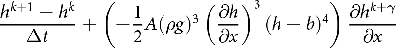 \begin{align*}
&\frac{h^{k+1}-h^k}{\Delta t}+\left(-\frac{1}{2}A(\rho g)^3 \left(\frac{\partial h}{\partial x}\right)^3 (h-b)^4\right) \frac{\partial h^{k+\gamma}}{\partial x}
\end{align*}
\begin{align*}
&\frac{h^{k+1}-h^k}{\Delta t}+\left(-\frac{1}{2}A(\rho g)^3 \left(\frac{\partial h}{\partial x}\right)^3 (h-b)^4\right) \frac{\partial h^{k+\gamma}}{\partial x}
\end{align*}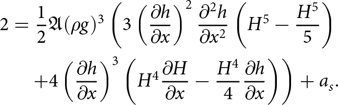 \begin{align}
{2}
&=\frac{1}{2}\mathfrak{A} (\rho g)^3\left(3 \left( \frac{\partial h}{\partial x} \right)^2 \frac{\partial^2 h}{\partial x^2} \left( H^5 -\frac{H^5}{5}\right) \right. \nonumber\\
&\quad \left.+4 \left( \frac{\partial h}{\partial x} \right)^3 \left(H^4 \frac{\partial H}{\partial x} -\frac{H^4}{4}\frac{\partial h}{\partial x}\right)\right) + a_s.
\end{align}
\begin{align}
{2}
&=\frac{1}{2}\mathfrak{A} (\rho g)^3\left(3 \left( \frac{\partial h}{\partial x} \right)^2 \frac{\partial^2 h}{\partial x^2} \left( H^5 -\frac{H^5}{5}\right) \right. \nonumber\\
&\quad \left.+4 \left( \frac{\partial h}{\partial x} \right)^3 \left(H^4 \frac{\partial H}{\partial x} -\frac{H^4}{4}\frac{\partial h}{\partial x}\right)\right) + a_s.
\end{align}This is a highly nonlinear equation and needs to be linearized before Fourier analysis can be used.
Without FSSA, all h and H-terms which do not have a superscript  $(\cdot)^{k+\gamma}$ are approximated explicitly, i.e. they all will have a superscript
  $(\cdot)^{k}$.
A.1.2. Linearization
Following Cheng and others Reference Cheng, Lotstedt and von Sydow(2017) (where the ice thickness equation was analysed), we consider a slab on a slope with a small surface perturbation δ around an average state  $\bar{h}$ which is just an inclined plane. We write:
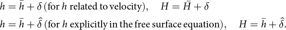 \begin{align*}
h&=\bar{h}+\delta \,\mathrm{(for}\ h\ \mathrm{related\,to\,velocity)}, \quad H=\bar{H}+\delta\\
h&=\bar{h}+\hat{\delta} \,\mathrm{(for}\ h\ \mathrm{explicitly\,in\,the\,free\,surface\,equation)} , \quad H=\bar{h}+\hat{\delta }.
\end{align*}
\begin{align*}
h&=\bar{h}+\delta \,\mathrm{(for}\ h\ \mathrm{related\,to\,velocity)}, \quad H=\bar{H}+\delta\\
h&=\bar{h}+\hat{\delta} \,\mathrm{(for}\ h\ \mathrm{explicitly\,in\,the\,free\,surface\,equation)} , \quad H=\bar{h}+\hat{\delta }.
\end{align*}Inserting in (A4) yields
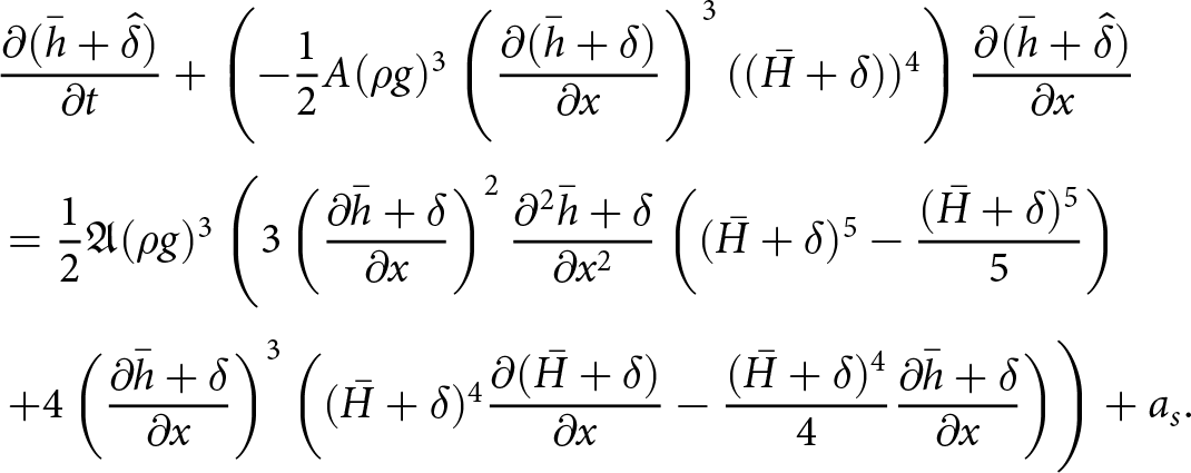 \begin{align*}
&\frac{\partial (\bar{h}+\hat{\delta})}{\partial t}+\left(-\frac{1}{2}A(\rho g)^3 \left(\frac{\partial (\bar{h}+\delta)}{\partial x}\right)^3 ((\bar{H}+\delta))^4\right) \frac{\partial (\bar{h}+\hat{\delta})}{\partial x} \\[3pt]
&= \frac{1}{2}\mathfrak{A} (\rho g)^3\left(3 \left( \frac{\partial \bar{h}+\delta}{\partial x} \right)^2 \frac{\partial^2 \bar{h}+\delta}{\partial x^2} \left( (\bar{H}+\delta)^5 -\frac{(\bar{H}+\delta)^5}{5}\right) \right.\\[3pt]
&\left.+4 \left( \frac{\partial \bar{h}+\delta}{\partial x} \right)^3 \left((\bar{H}+\delta)^4 \frac{\partial (\bar{H}+\delta)}{\partial x} -\frac{(\bar{H}+\delta)^4}{4}\frac{\partial \bar{h}+\delta }{\partial x}\right)\right) + a_s.
\end{align*}
\begin{align*}
&\frac{\partial (\bar{h}+\hat{\delta})}{\partial t}+\left(-\frac{1}{2}A(\rho g)^3 \left(\frac{\partial (\bar{h}+\delta)}{\partial x}\right)^3 ((\bar{H}+\delta))^4\right) \frac{\partial (\bar{h}+\hat{\delta})}{\partial x} \\[3pt]
&= \frac{1}{2}\mathfrak{A} (\rho g)^3\left(3 \left( \frac{\partial \bar{h}+\delta}{\partial x} \right)^2 \frac{\partial^2 \bar{h}+\delta}{\partial x^2} \left( (\bar{H}+\delta)^5 -\frac{(\bar{H}+\delta)^5}{5}\right) \right.\\[3pt]
&\left.+4 \left( \frac{\partial \bar{h}+\delta}{\partial x} \right)^3 \left((\bar{H}+\delta)^4 \frac{\partial (\bar{H}+\delta)}{\partial x} -\frac{(\bar{H}+\delta)^4}{4}\frac{\partial \bar{h}+\delta }{\partial x}\right)\right) + a_s.
\end{align*} Using that the second derivative of the steady state surface  $\bar{h}$ is zero we get
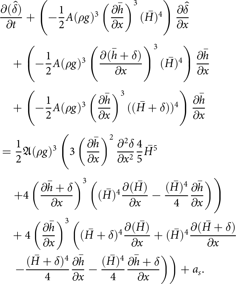 \begin{align*}
&\frac{\partial (\hat{\delta})}{\partial t}+\left(-\frac{1}{2}A(\rho g)^3 \left(\frac{\partial \bar{h}}{\partial x}\right)^3 (\bar{H})^4\right) \frac{\partial \hat{\delta}}{\partial x} \\[3pt]
&\quad +\left(-\frac{1}{2}A(\rho g)^3 \left(\frac{\partial (\bar{h}+\delta)}{\partial x}\right)^3 (\bar{H})^4\right) \frac{\partial \bar{h}}{\partial x} \\[3pt]
&\quad +\left(-\frac{1}{2}A(\rho g)^3 \left(\frac{\partial \bar{h}}{\partial x}\right)^3 ((\bar{H}+\delta))^4\right) \frac{\partial \bar{h}}{\partial x} \\[3pt]
&= \frac{1}{2}\mathfrak{A} (\rho g)^3\left(3 \left( \frac{\partial \bar{h}}{\partial x} \right)^2 \frac{\partial^2 \delta}{\partial x^2} \frac{4}{5}\bar{H}^5 \right.\\[3pt]
&\quad \left.+4 \left( \frac{\partial \bar{h}+\delta}{\partial x} \right)^3 \left((\bar{H})^4 \frac{\partial (\bar{H})}{\partial x} -\frac{(\bar{H})^4}{4}\frac{\partial \bar{h} }{\partial x}\right)\right) \\
&\quad +4 \left( \frac{\partial \bar{h}}{\partial x} \right)^3 \left((\bar{H}+\delta)^4 \frac{\partial (\bar{H})}{\partial x}+(\bar{H})^4 \frac{\partial (\bar{H}+\delta)}{\partial x} \right.\\
&\quad \left.\left.-\frac{(\bar{H}+\delta)^4}{4}\frac{\partial \bar{h} }{\partial x} -\frac{(\bar{H})^4}{4}\frac{\partial \bar{h}+\delta }{\partial x}\right)\right) + a_s.
\end{align*}
\begin{align*}
&\frac{\partial (\hat{\delta})}{\partial t}+\left(-\frac{1}{2}A(\rho g)^3 \left(\frac{\partial \bar{h}}{\partial x}\right)^3 (\bar{H})^4\right) \frac{\partial \hat{\delta}}{\partial x} \\[3pt]
&\quad +\left(-\frac{1}{2}A(\rho g)^3 \left(\frac{\partial (\bar{h}+\delta)}{\partial x}\right)^3 (\bar{H})^4\right) \frac{\partial \bar{h}}{\partial x} \\[3pt]
&\quad +\left(-\frac{1}{2}A(\rho g)^3 \left(\frac{\partial \bar{h}}{\partial x}\right)^3 ((\bar{H}+\delta))^4\right) \frac{\partial \bar{h}}{\partial x} \\[3pt]
&= \frac{1}{2}\mathfrak{A} (\rho g)^3\left(3 \left( \frac{\partial \bar{h}}{\partial x} \right)^2 \frac{\partial^2 \delta}{\partial x^2} \frac{4}{5}\bar{H}^5 \right.\\[3pt]
&\quad \left.+4 \left( \frac{\partial \bar{h}+\delta}{\partial x} \right)^3 \left((\bar{H})^4 \frac{\partial (\bar{H})}{\partial x} -\frac{(\bar{H})^4}{4}\frac{\partial \bar{h} }{\partial x}\right)\right) \\
&\quad +4 \left( \frac{\partial \bar{h}}{\partial x} \right)^3 \left((\bar{H}+\delta)^4 \frac{\partial (\bar{H})}{\partial x}+(\bar{H})^4 \frac{\partial (\bar{H}+\delta)}{\partial x} \right.\\
&\quad \left.\left.-\frac{(\bar{H}+\delta)^4}{4}\frac{\partial \bar{h} }{\partial x} -\frac{(\bar{H})^4}{4}\frac{\partial \bar{h}+\delta }{\partial x}\right)\right) + a_s.
\end{align*}Ignoring higher order terms in δ furthermore yields
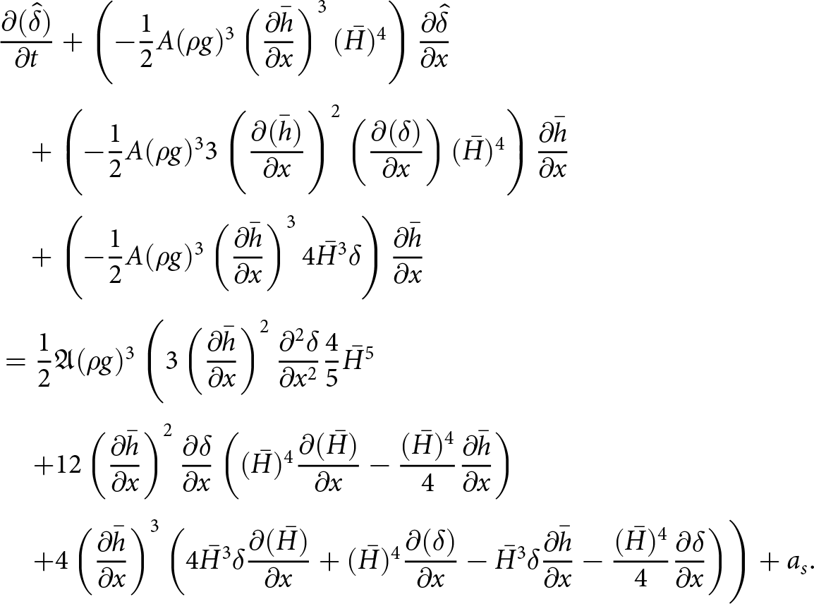 \begin{align*}
&\frac{\partial (\hat{\delta})}{\partial t}+\left(-\frac{1}{2}A(\rho g)^3 \left(\frac{\partial \bar{h}}{\partial x}\right)^3 (\bar{H})^4\right) \frac{\partial \hat{\delta}}{\partial x} \\[3pt]
&\quad +\left(-\frac{1}{2}A(\rho g)^3 3\left(\frac{\partial (\bar{h})}{\partial x}\right)^2\left(\frac{\partial (\delta)}{\partial x}\right) (\bar{H})^4\right) \frac{\partial \bar{h}}{\partial x} \\[3pt]
&\quad +\left(-\frac{1}{2}A(\rho g)^3 \left(\frac{\partial \bar{h}}{\partial x}\right)^3 4\bar{H}^3\delta \right) \frac{\partial \bar{h}}{\partial x} \\[3pt]
&= \frac{1}{2}\mathfrak{A} (\rho g)^3\left(3 \left( \frac{\partial \bar{h}}{\partial x} \right)^2 \frac{\partial^2 \delta}{\partial x^2} \frac{4}{5}\bar{H}^5 \right.\\[3pt]
&\quad \left.+12 \left( \frac{\partial \bar{h}}{\partial x} \right)^2 \frac{\partial \delta}{\partial x} \left((\bar{H})^4 \frac{\partial (\bar{H})}{\partial x} -\frac{(\bar{H})^4}{4}\frac{\partial \bar{h} }{\partial x}\right)\right. \\[3pt]
&\left.\quad +4 \left( \frac{\partial \bar{h}}{\partial x} \right)^3 \left(4\bar{H}^3\delta \frac{\partial (\bar{H})}{\partial x}+(\bar{H})^4 \frac{\partial (\delta)}{\partial x} -\bar{H}^3\delta \frac{\partial \bar{h} }{\partial x}-\frac{(\bar{H})^4}{4}\frac{\partial \delta }{\partial x}\right)\right) + a_s.
\end{align*}
\begin{align*}
&\frac{\partial (\hat{\delta})}{\partial t}+\left(-\frac{1}{2}A(\rho g)^3 \left(\frac{\partial \bar{h}}{\partial x}\right)^3 (\bar{H})^4\right) \frac{\partial \hat{\delta}}{\partial x} \\[3pt]
&\quad +\left(-\frac{1}{2}A(\rho g)^3 3\left(\frac{\partial (\bar{h})}{\partial x}\right)^2\left(\frac{\partial (\delta)}{\partial x}\right) (\bar{H})^4\right) \frac{\partial \bar{h}}{\partial x} \\[3pt]
&\quad +\left(-\frac{1}{2}A(\rho g)^3 \left(\frac{\partial \bar{h}}{\partial x}\right)^3 4\bar{H}^3\delta \right) \frac{\partial \bar{h}}{\partial x} \\[3pt]
&= \frac{1}{2}\mathfrak{A} (\rho g)^3\left(3 \left( \frac{\partial \bar{h}}{\partial x} \right)^2 \frac{\partial^2 \delta}{\partial x^2} \frac{4}{5}\bar{H}^5 \right.\\[3pt]
&\quad \left.+12 \left( \frac{\partial \bar{h}}{\partial x} \right)^2 \frac{\partial \delta}{\partial x} \left((\bar{H})^4 \frac{\partial (\bar{H})}{\partial x} -\frac{(\bar{H})^4}{4}\frac{\partial \bar{h} }{\partial x}\right)\right. \\[3pt]
&\left.\quad +4 \left( \frac{\partial \bar{h}}{\partial x} \right)^3 \left(4\bar{H}^3\delta \frac{\partial (\bar{H})}{\partial x}+(\bar{H})^4 \frac{\partial (\delta)}{\partial x} -\bar{H}^3\delta \frac{\partial \bar{h} }{\partial x}-\frac{(\bar{H})^4}{4}\frac{\partial \delta }{\partial x}\right)\right) + a_s.
\end{align*}Considering that the steady state thickness is zero further simplifies the expression into
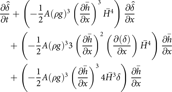 \begin{align*}
&\frac{\partial \hat{\delta}}{\partial t}+\left(-\frac{1}{2}A(\rho g)^3 \left(\frac{\partial \bar{h}}{\partial x}\right)^3 \bar{H}^4\right) \frac{\partial \hat{\delta}}{\partial x}\\
&\quad +\left(-\frac{1}{2}A(\rho g)^3 3\left(\frac{\partial \bar{h}}{\partial x}\right)^2\left(\frac{\partial (\delta)}{\partial x}\right) \bar{H}^4\right) \frac{\partial \bar{h}}{\partial x} \\
&\quad +\left(-\frac{1}{2}A(\rho g)^3 \left(\frac{\partial \bar{h}}{\partial x}\right)^3 4\bar{H}^3\delta \right) \frac{\partial \bar{h}}{\partial x}
\end{align*}
\begin{align*}
&\frac{\partial \hat{\delta}}{\partial t}+\left(-\frac{1}{2}A(\rho g)^3 \left(\frac{\partial \bar{h}}{\partial x}\right)^3 \bar{H}^4\right) \frac{\partial \hat{\delta}}{\partial x}\\
&\quad +\left(-\frac{1}{2}A(\rho g)^3 3\left(\frac{\partial \bar{h}}{\partial x}\right)^2\left(\frac{\partial (\delta)}{\partial x}\right) \bar{H}^4\right) \frac{\partial \bar{h}}{\partial x} \\
&\quad +\left(-\frac{1}{2}A(\rho g)^3 \left(\frac{\partial \bar{h}}{\partial x}\right)^3 4\bar{H}^3\delta \right) \frac{\partial \bar{h}}{\partial x}
\end{align*}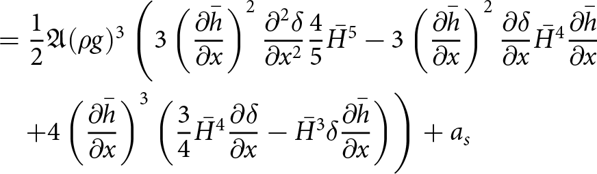 \begin{align*}
&= \frac{1}{2}\mathfrak{A} (\rho g)^3\left(3 \left( \frac{\partial \bar{h}}{\partial x} \right)^2 \frac{\partial^2 \delta}{\partial x^2} \frac{4}{5}\bar{H}^5 -3 \left( \frac{\partial \bar{h}}{\partial x} \right)^2 \frac{\partial \delta}{\partial x} \bar{H}^4\frac{\partial \bar{h} }{\partial x} \right.\\
&\quad \left.+4 \left( \frac{\partial \bar{h}}{\partial x} \right)^3 \left(\frac{3}{4}\bar{H}^4 \frac{\partial \delta}{\partial x} -\bar{H}^3\delta \frac{\partial \bar{h} }{\partial x}\right)\right) + a_s
\end{align*}
\begin{align*}
&= \frac{1}{2}\mathfrak{A} (\rho g)^3\left(3 \left( \frac{\partial \bar{h}}{\partial x} \right)^2 \frac{\partial^2 \delta}{\partial x^2} \frac{4}{5}\bar{H}^5 -3 \left( \frac{\partial \bar{h}}{\partial x} \right)^2 \frac{\partial \delta}{\partial x} \bar{H}^4\frac{\partial \bar{h} }{\partial x} \right.\\
&\quad \left.+4 \left( \frac{\partial \bar{h}}{\partial x} \right)^3 \left(\frac{3}{4}\bar{H}^4 \frac{\partial \delta}{\partial x} -\bar{H}^3\delta \frac{\partial \bar{h} }{\partial x}\right)\right) + a_s
\end{align*} rearranging and defining 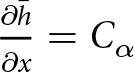 $\frac{\partial \bar{h}}{\partial x}=C_\alpha$ we get:
 \begin{align*}
&\frac{\partial \hat{\delta}}{\partial t}-\frac{1}{2}\mathfrak{A}(\rho g)^3 C_\alpha^3 \bar{H}^4 \frac{\partial \hat{\delta}}{\partial x} -\frac{3}{2}\mathfrak{A}(\rho g)^3 C_\alpha^3 \bar{H}^4 \frac{\partial \delta}{\partial x} = \frac{6}{5}\mathfrak{A} (\rho g)^3 C_\alpha^2 \bar{H}^5 \frac{\partial^2 \delta}{\partial x^2} + a_s
\end{align*}
\begin{align*}
&\frac{\partial \hat{\delta}}{\partial t}-\frac{1}{2}\mathfrak{A}(\rho g)^3 C_\alpha^3 \bar{H}^4 \frac{\partial \hat{\delta}}{\partial x} -\frac{3}{2}\mathfrak{A}(\rho g)^3 C_\alpha^3 \bar{H}^4 \frac{\partial \delta}{\partial x} = \frac{6}{5}\mathfrak{A} (\rho g)^3 C_\alpha^2 \bar{H}^5 \frac{\partial^2 \delta}{\partial x^2} + a_s
\end{align*}which we will write on the form
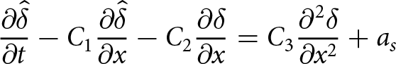 \begin{align*}
&\frac{\partial \hat{\delta}}{\partial t}-C_1 \frac{\partial \hat{\delta}}{\partial x} -C_2 \frac{\partial \delta}{\partial x} = C_3\frac{\partial^2 \delta}{\partial x^2} + a_s
\end{align*}
\begin{align*}
&\frac{\partial \hat{\delta}}{\partial t}-C_1 \frac{\partial \hat{\delta}}{\partial x} -C_2 \frac{\partial \delta}{\partial x} = C_3\frac{\partial^2 \delta}{\partial x^2} + a_s
\end{align*} with  $C_1=\frac{1}{2}\mathfrak{A}(\rho g)^3 C_\alpha^3 \bar{H}^4$,
  $C_2= \frac{3}{2}\mathfrak{A}(\rho g)^3 C_\alpha^3 \bar{H}^4$ and
  $C_3=\frac{6}{5}\mathfrak{A} (\rho g)^3 C_\alpha^2 \bar{H}^5 $. OBS! C 1 and C 2 are negative!
We can discretize  $\hat{\delta}$ using k or k + 1 (the latter is better of course), while δ must be taken from time step k as it originates from the velocity.
A.1.3. Fourier analysis
We will now consider the SIA solution in Fourier space. We will thus apply a Fourier transform, and consider one frequency at a time
 \begin{align*}
\delta^k_j \rightarrow \tilde{\delta}^k \mathrm{e}^{i n x_j}=\tilde{\delta} \mathrm{e}^{i n j \Delta x}\\
\delta^k_{j+1} \rightarrow \tilde{\delta}^k \mathrm{e}^{i n x_{j+1}}=\tilde{\delta}^k \mathrm{e}^{i n j \Delta x}e^{i n \Delta x}.
\end{align*}
\begin{align*}
\delta^k_j \rightarrow \tilde{\delta}^k \mathrm{e}^{i n x_j}=\tilde{\delta} \mathrm{e}^{i n j \Delta x}\\
\delta^k_{j+1} \rightarrow \tilde{\delta}^k \mathrm{e}^{i n x_{j+1}}=\tilde{\delta}^k \mathrm{e}^{i n j \Delta x}e^{i n \Delta x}.
\end{align*} The factor  $\mathrm{e}^{i n j \Delta x}$ will appear in every term of every equation, and we will hence divide by that and not write it out from here on. We will also consider the finite difference discretization which best corresponds to a P1 FEM discretization, meaning that second derivatives will be represented as central differences so that
  $\frac{\partial \delta}{\partial x}$ and
  $\frac{\partial^2 \delta}{\partial x^2} $ are discretized and transformed as:
 \begin{align*}
\frac{\partial \delta}{\partial x} \approx \frac{\delta_{j+1}-\delta_{j-1}}{2 \Delta x} \rightarrow \tilde{\delta}\frac{\mathrm{e}^{in \Delta x}-\mathrm{e}^{-in \Delta x}}{2 \Delta x} = \tilde{\delta}\frac{2i \mathrm{sin} (n\Delta x)}{2 \Delta x}\\
\frac{\partial^2 \delta}{\partial x^2}\approx \frac{\delta_{j+1}-2\delta_{j}+\delta_{j-1}}{(\Delta x)^2} \rightarrow \tilde{\delta} \frac{ \mathrm{e}^{in \Delta x}-2+\mathrm{e}^{-in \Delta x} }{(\Delta x)^2} = -\tilde{\delta}\frac{4 \sin^2 (n \Delta x/2)}{(\Delta x)^2 }.
\end{align*}
\begin{align*}
\frac{\partial \delta}{\partial x} \approx \frac{\delta_{j+1}-\delta_{j-1}}{2 \Delta x} \rightarrow \tilde{\delta}\frac{\mathrm{e}^{in \Delta x}-\mathrm{e}^{-in \Delta x}}{2 \Delta x} = \tilde{\delta}\frac{2i \mathrm{sin} (n\Delta x)}{2 \Delta x}\\
\frac{\partial^2 \delta}{\partial x^2}\approx \frac{\delta_{j+1}-2\delta_{j}+\delta_{j-1}}{(\Delta x)^2} \rightarrow \tilde{\delta} \frac{ \mathrm{e}^{in \Delta x}-2+\mathrm{e}^{-in \Delta x} }{(\Delta x)^2} = -\tilde{\delta}\frac{4 \sin^2 (n \Delta x/2)}{(\Delta x)^2 }.
\end{align*} Inserting this into the linearized equation, assuming implicit handling of the free-surface equation α = 1 itself and explicit handling of velocities, and setting  $a_s=0$ gives
 \begin{align*}
&\frac{\tilde{\delta}^{k+1}-\tilde{\delta}^{k}}{\Delta t}-C_1 \tilde{\delta}^{k+1}\frac{2i \mathrm{sin} (n\Delta x)}{2 \Delta x} -C_2 \tilde{\delta}^{k}\frac{2i \mathrm{sin} (n\Delta x)}{2 \Delta x} =- C_3 \tilde{\delta^k}\frac{4 \sin^2 (n \Delta x/2)}{(\Delta x)^2 }.
\end{align*}
\begin{align*}
&\frac{\tilde{\delta}^{k+1}-\tilde{\delta}^{k}}{\Delta t}-C_1 \tilde{\delta}^{k+1}\frac{2i \mathrm{sin} (n\Delta x)}{2 \Delta x} -C_2 \tilde{\delta}^{k}\frac{2i \mathrm{sin} (n\Delta x)}{2 \Delta x} =- C_3 \tilde{\delta^k}\frac{4 \sin^2 (n \Delta x/2)}{(\Delta x)^2 }.
\end{align*}Using Euler’s formulas and rearranging gives:
 \begin{align*}
&\tilde{\delta}^{k+1} \left(1 -\Delta t C_1 \frac{2i \mathrm{sin} (n\Delta x)}{2 \Delta x} \right) \\
&\quad =\tilde{\delta}^{k} \left(1 - \Delta tC_3 \frac{4 \sin^2 (n \Delta x/2)}{(\Delta x)^2 }+ \Delta t C_2 \frac{2i \mathrm{sin} (n\Delta x)}{2 \Delta x} \right) .
\end{align*}
\begin{align*}
&\tilde{\delta}^{k+1} \left(1 -\Delta t C_1 \frac{2i \mathrm{sin} (n\Delta x)}{2 \Delta x} \right) \\
&\quad =\tilde{\delta}^{k} \left(1 - \Delta tC_3 \frac{4 \sin^2 (n \Delta x/2)}{(\Delta x)^2 }+ \Delta t C_2 \frac{2i \mathrm{sin} (n\Delta x)}{2 \Delta x} \right) .
\end{align*} In order for each Fourier mode to stay bounded as the simulation runs, i.e. that  $|\tilde{\delta}^{k+1}|\leq |\tilde{\delta}^{k}|$, we require that
 \begin{equation}
\frac{\left|1 - \Delta tC_3 \frac{4 \sin^2 (n \Delta x/2)}{(\Delta x)^2 }+ \Delta t C_2 \frac{2i \mathrm{sin} (n\Delta x)}{2 \Delta x} \right| }{\left|1 -\Delta t C_1 \frac{2i \mathrm{sin} (n\Delta x)}{2 \Delta x} \right|} \leq 1.
\end{equation}
\begin{equation}
\frac{\left|1 - \Delta tC_3 \frac{4 \sin^2 (n \Delta x/2)}{(\Delta x)^2 }+ \Delta t C_2 \frac{2i \mathrm{sin} (n\Delta x)}{2 \Delta x} \right| }{\left|1 -\Delta t C_1 \frac{2i \mathrm{sin} (n\Delta x)}{2 \Delta x} \right|} \leq 1.
\end{equation}The denominator value of the parenthesis of the left-hand side is always larger than one (which is due to that α = 1). We thus only need to bound the nominator. The complex part of the nominator is bounded as long as
 \begin{align*}
\frac{|C_2| \Delta t }{2\Delta t}\leq 1,
\end{align*}
\begin{align*}
\frac{|C_2| \Delta t }{2\Delta t}\leq 1,
\end{align*}while the real part needs to fulfil
 \begin{align*}
\left|1 - \Delta tC_3 \frac{4 \sin^2 (n \Delta x/2)}{(\Delta x)^2 }\right| \lt 1 \Rightarrow \frac{C_3\Delta t}{(\Delta x)^2} \lt 0.5.
\end{align*}
\begin{align*}
\left|1 - \Delta tC_3 \frac{4 \sin^2 (n \Delta x/2)}{(\Delta x)^2 }\right| \lt 1 \Rightarrow \frac{C_3\Delta t}{(\Delta x)^2} \lt 0.5.
\end{align*}So depending on the balance between C 2 and C 3, we get a linear or parabolic time-step constraint. C 3 is big for thick ice with flat slopes, i.e. for the dynamics typical of the interior of an ice sheet, we get a parabolic constraint.
A.2. With FSSA
A.2.1. Coupling
As observed from (32), the addition of the FSSA terms makes the discretization of the pressure implicit:
 \begin{equation}
p(x,y,t) \approx \rho g (h^{k+1} - y).
\end{equation}
\begin{equation}
p(x,y,t) \approx \rho g (h^{k+1} - y).
\end{equation}The pressure yields u 1 and u 1 gives u 2, so this implicit discretization will propagate to the velocity solution in the following way
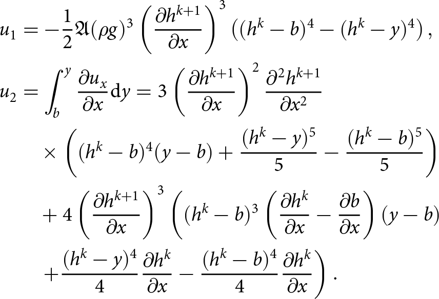 \begin{align*}
u_1 &= - \frac{1}{2}\mathfrak{A} (\rho g)^3 \left(\frac{\partial h^{k+1}}{\partial x}\right)^3 \left( (h^k-b)^4- (h^k-y)^4 \right),\\
u_2 & =\int_b^y \frac{\partial u_x}{\partial x} \mathrm{d}y = 3 \left( \frac{\partial h^{k+1}}{\partial x} \right)^2 \frac{\partial^2 h^{k+1}}{\partial x^2} \\
&\quad \times \left( (h^k-b)^4 (y-b)+\frac{(h^k-y)^5}{5}-\frac{(h^k-b)^5}{5}\right) \\
& \quad +4 \left( \frac{\partial h^{k+1}}{\partial x} \right)^3 \left((h^k-b)^3\left( \frac{\partial h^k}{\partial x}-\frac{\partial b}{\partial x} \right) (y-b) \right.\\
&\quad \left. + \frac{(h^k-y)^4}{4}\frac{\partial h^k}{\partial x}-\frac{(h^k-b)^4}{4}\frac{\partial h^k}{\partial x}\right).
\end{align*}
\begin{align*}
u_1 &= - \frac{1}{2}\mathfrak{A} (\rho g)^3 \left(\frac{\partial h^{k+1}}{\partial x}\right)^3 \left( (h^k-b)^4- (h^k-y)^4 \right),\\
u_2 & =\int_b^y \frac{\partial u_x}{\partial x} \mathrm{d}y = 3 \left( \frac{\partial h^{k+1}}{\partial x} \right)^2 \frac{\partial^2 h^{k+1}}{\partial x^2} \\
&\quad \times \left( (h^k-b)^4 (y-b)+\frac{(h^k-y)^5}{5}-\frac{(h^k-b)^5}{5}\right) \\
& \quad +4 \left( \frac{\partial h^{k+1}}{\partial x} \right)^3 \left((h^k-b)^3\left( \frac{\partial h^k}{\partial x}-\frac{\partial b}{\partial x} \right) (y-b) \right.\\
&\quad \left. + \frac{(h^k-y)^4}{4}\frac{\partial h^k}{\partial x}-\frac{(h^k-b)^4}{4}\frac{\partial h^k}{\partial x}\right).
\end{align*}Then the final expressions at y = h are:
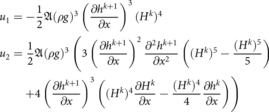 \begin{align*}
u_1 &=- \frac{1}{2}\mathfrak{A} (\rho g)^3 \left(\frac{\partial h^{k+1}}{\partial x}\right)^3 (H^k)^4 \\
u_2&=\frac{1}{2}\mathfrak{A} (\rho g)^3\left(3 \left( \frac{\partial h^{k+1}}{\partial x} \right)^2 \frac{\partial^2 h^{k+1}}{\partial x^2} \left( (H^k)^5 -\frac{(H^k)^5}{5}\right)\right.\\
&\quad \left. +4 \left( \frac{\partial h^{k+1}}{\partial x} \right)^3 \left((H^k)^4 \frac{\partial H^k}{\partial x} -\frac{(H^k)^4}{4}\frac{\partial h^k}{\partial x}\right)\right)
\end{align*}
\begin{align*}
u_1 &=- \frac{1}{2}\mathfrak{A} (\rho g)^3 \left(\frac{\partial h^{k+1}}{\partial x}\right)^3 (H^k)^4 \\
u_2&=\frac{1}{2}\mathfrak{A} (\rho g)^3\left(3 \left( \frac{\partial h^{k+1}}{\partial x} \right)^2 \frac{\partial^2 h^{k+1}}{\partial x^2} \left( (H^k)^5 -\frac{(H^k)^5}{5}\right)\right.\\
&\quad \left. +4 \left( \frac{\partial h^{k+1}}{\partial x} \right)^3 \left((H^k)^4 \frac{\partial H^k}{\partial x} -\frac{(H^k)^4}{4}\frac{\partial h^k}{\partial x}\right)\right)
\end{align*}and the fully coupled system is then
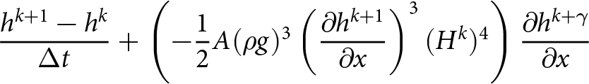 \begin{align*}
&\frac{h^{k+1}-h^k}{\Delta t}+\left(-\frac{1}{2}A(\rho g)^3 \left(\frac{\partial h^{k+1}}{\partial x}\right)^3 (H^k)^4\right) \frac{\partial h^{k+\gamma}}{\partial x}
\end{align*}
\begin{align*}
&\frac{h^{k+1}-h^k}{\Delta t}+\left(-\frac{1}{2}A(\rho g)^3 \left(\frac{\partial h^{k+1}}{\partial x}\right)^3 (H^k)^4\right) \frac{\partial h^{k+\gamma}}{\partial x}
\end{align*}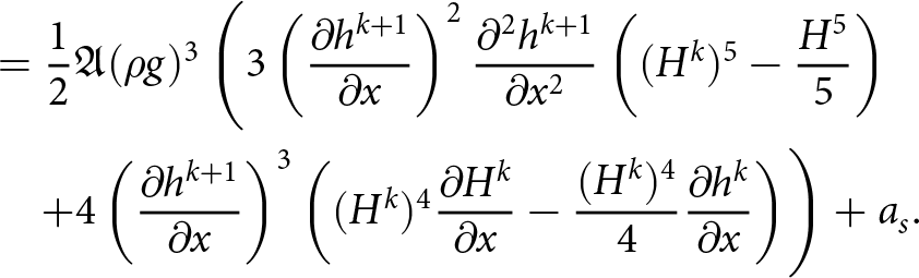 \begin{alignat}{2}
&=\frac{1}{2}\mathfrak{A} (\rho g)^3\left(3 \left( \frac{\partial h^{k+1}}{\partial x} \right)^2 \frac{\partial^2 h^{k+1}}{\partial x^2} \left( (H^k)^5 -\frac{H^5}{5}\right) \right.\nonumber\\
&\quad \left.+4 \left( \frac{\partial h^{k+1}}{\partial x} \right)^3 \left((H^k)^4 \frac{\partial H^k}{\partial x} -\frac{(H^k)^4}{4}\frac{\partial h^k}{\partial x}\right)\right) + a_s.
\end{alignat}
\begin{alignat}{2}
&=\frac{1}{2}\mathfrak{A} (\rho g)^3\left(3 \left( \frac{\partial h^{k+1}}{\partial x} \right)^2 \frac{\partial^2 h^{k+1}}{\partial x^2} \left( (H^k)^5 -\frac{H^5}{5}\right) \right.\nonumber\\
&\quad \left.+4 \left( \frac{\partial h^{k+1}}{\partial x} \right)^3 \left((H^k)^4 \frac{\partial H^k}{\partial x} -\frac{(H^k)^4}{4}\frac{\partial h^k}{\partial x}\right)\right) + a_s.
\end{alignat}A.2.2. Linearization
With the same approach as before we get
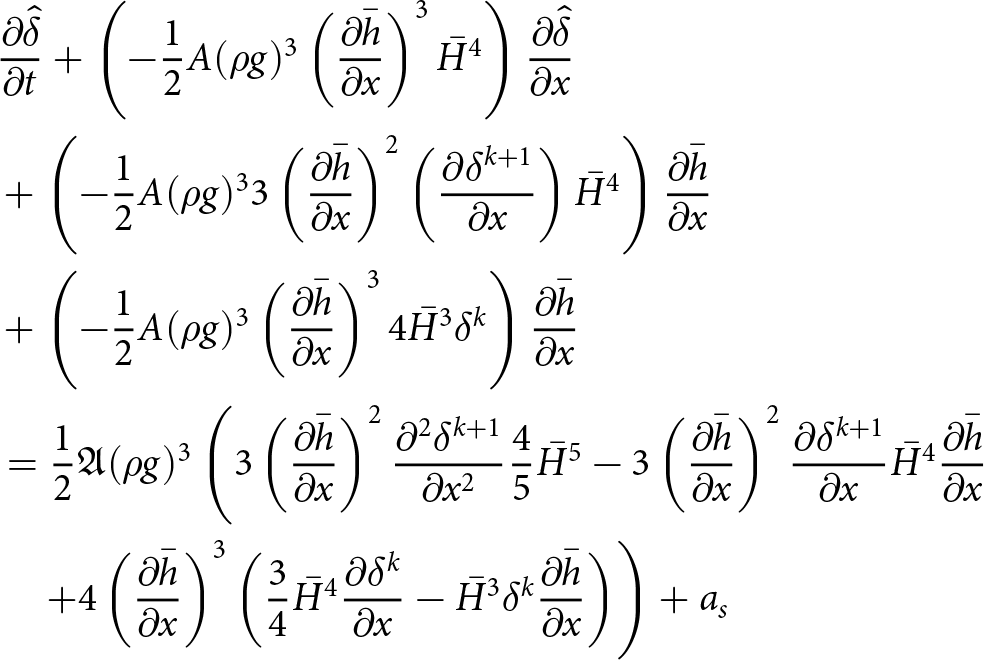 \begin{align*}
&\frac{\partial \hat{\delta}}{\partial t}+\left(-\frac{1}{2}A(\rho g)^3 \left(\frac{\partial \bar{h}}{\partial x}\right)^3 \bar{H}^4\right) \frac{\partial \hat{\delta}}{\partial x} \\
&+\left(-\frac{1}{2}A(\rho g)^3 3\left(\frac{\partial \bar{h}}{\partial x}\right)^2\left(\frac{\partial \delta^{k+1}}{\partial x}\right) \bar{H}^4\right) \frac{\partial \bar{h}}{\partial x} \\
&+\left(-\frac{1}{2}A(\rho g)^3 \left(\frac{\partial \bar{h}}{\partial x}\right)^3 4\bar{H}^3\delta^k \right) \frac{\partial \bar{h}}{\partial x} \\
&= \frac{1}{2}\mathfrak{A} (\rho g)^3\left(3 \left( \frac{\partial \bar{h}}{\partial x} \right)^2 \frac{\partial^2 \delta^{k+1}}{\partial x^2} \frac{4}{5}\bar{H}^5 -3 \left( \frac{\partial \bar{h}}{\partial x} \right)^2 \frac{\partial \delta^{k+1}}{\partial x} \bar{H}^4\frac{\partial \bar{h} }{\partial x} \right.\\
&\quad \left.+4 \left( \frac{\partial \bar{h}}{\partial x} \right)^3 \left(\frac{3}{4}\bar{H}^4 \frac{\partial \delta^k}{\partial x} -\bar{H}^3\delta^k \frac{\partial \bar{h} }{\partial x}\right)\right) + a_s
\end{align*}
\begin{align*}
&\frac{\partial \hat{\delta}}{\partial t}+\left(-\frac{1}{2}A(\rho g)^3 \left(\frac{\partial \bar{h}}{\partial x}\right)^3 \bar{H}^4\right) \frac{\partial \hat{\delta}}{\partial x} \\
&+\left(-\frac{1}{2}A(\rho g)^3 3\left(\frac{\partial \bar{h}}{\partial x}\right)^2\left(\frac{\partial \delta^{k+1}}{\partial x}\right) \bar{H}^4\right) \frac{\partial \bar{h}}{\partial x} \\
&+\left(-\frac{1}{2}A(\rho g)^3 \left(\frac{\partial \bar{h}}{\partial x}\right)^3 4\bar{H}^3\delta^k \right) \frac{\partial \bar{h}}{\partial x} \\
&= \frac{1}{2}\mathfrak{A} (\rho g)^3\left(3 \left( \frac{\partial \bar{h}}{\partial x} \right)^2 \frac{\partial^2 \delta^{k+1}}{\partial x^2} \frac{4}{5}\bar{H}^5 -3 \left( \frac{\partial \bar{h}}{\partial x} \right)^2 \frac{\partial \delta^{k+1}}{\partial x} \bar{H}^4\frac{\partial \bar{h} }{\partial x} \right.\\
&\quad \left.+4 \left( \frac{\partial \bar{h}}{\partial x} \right)^3 \left(\frac{3}{4}\bar{H}^4 \frac{\partial \delta^k}{\partial x} -\bar{H}^3\delta^k \frac{\partial \bar{h} }{\partial x}\right)\right) + a_s
\end{align*} rearranging and setting  $\frac{\partial \bar{h}}{\partial x}=\frac{\partial \bar{h}}{\partial x}=C_\alpha$ yields
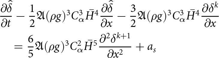 \begin{align*}
&\frac{\partial \hat{\delta}}{\partial t}-\frac{1}{2}\mathfrak{A}(\rho g)^3 C_\alpha^3 \bar{H}^4 \frac{\partial \hat{\delta}}{\partial x} -\frac{3}{2}\mathfrak{A}(\rho g)^3 C_\alpha^3 \bar{H}^4 \frac{\partial \delta^{k}}{\partial x} \\
&\quad = \frac{6}{5}\mathfrak{A} (\rho g)^3 C_\alpha^2 \bar{H}^5 \frac{\partial^2 \delta^{k+1}}{\partial x^2} + a_s
\end{align*}
\begin{align*}
&\frac{\partial \hat{\delta}}{\partial t}-\frac{1}{2}\mathfrak{A}(\rho g)^3 C_\alpha^3 \bar{H}^4 \frac{\partial \hat{\delta}}{\partial x} -\frac{3}{2}\mathfrak{A}(\rho g)^3 C_\alpha^3 \bar{H}^4 \frac{\partial \delta^{k}}{\partial x} \\
&\quad = \frac{6}{5}\mathfrak{A} (\rho g)^3 C_\alpha^2 \bar{H}^5 \frac{\partial^2 \delta^{k+1}}{\partial x^2} + a_s
\end{align*}which we will write on the form
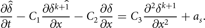 \begin{align*}
&\frac{\partial \hat{\delta}}{\partial t}-C_1 \frac{\partial \hat{\delta^{k+1}}}{\partial x} -C_2 \frac{\partial \delta}{\partial x} = C_3\frac{\partial^2 \delta^{k+1}}{\partial x^2} + a_s.
\end{align*}
\begin{align*}
&\frac{\partial \hat{\delta}}{\partial t}-C_1 \frac{\partial \hat{\delta^{k+1}}}{\partial x} -C_2 \frac{\partial \delta}{\partial x} = C_3\frac{\partial^2 \delta^{k+1}}{\partial x^2} + a_s.
\end{align*}So the difference in the linearized equation is that the second derivative is treated implicitly.
A.2.3. Fourier analysis
We get the same expression as without FSSA, only that the second derivative is now treated implicitly
 \begin{align*}
&\frac{\tilde{\delta}^{k+1}-\tilde{\delta}^{k}}{\Delta t}-C_1 \tilde{\delta}^{k+1}\frac{2i \mathrm{sin} (n\Delta x)}{2 \Delta x} -C_2 \tilde{\delta}^{k}\frac{2i \mathrm{sin} (n\Delta x)}{2 \Delta x} =- C_3 \tilde{\delta^k}\frac{4 \sin^2 (n \Delta x/2)}{(\Delta x)^2 }.
\end{align*}
\begin{align*}
&\frac{\tilde{\delta}^{k+1}-\tilde{\delta}^{k}}{\Delta t}-C_1 \tilde{\delta}^{k+1}\frac{2i \mathrm{sin} (n\Delta x)}{2 \Delta x} -C_2 \tilde{\delta}^{k}\frac{2i \mathrm{sin} (n\Delta x)}{2 \Delta x} =- C_3 \tilde{\delta^k}\frac{4 \sin^2 (n \Delta x/2)}{(\Delta x)^2 }.
\end{align*}Rearranging gives
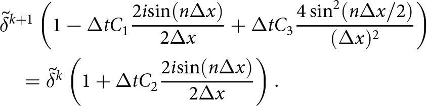 \begin{align*}
&\tilde{\delta}^{k+1} \left(1 -\Delta t C_1 \frac{2i \mathrm{sin} (n\Delta x)}{2 \Delta x}+ \Delta tC_3 \frac{4 \sin^2 (n \Delta x/2)}{(\Delta x)^2 } \right) \\
&\quad =\tilde{\delta}^{k} \left(1 + \Delta t C_2 \frac{2i \mathrm{sin} (n\Delta x)}{2 \Delta x} \right).
\end{align*}
\begin{align*}
&\tilde{\delta}^{k+1} \left(1 -\Delta t C_1 \frac{2i \mathrm{sin} (n\Delta x)}{2 \Delta x}+ \Delta tC_3 \frac{4 \sin^2 (n \Delta x/2)}{(\Delta x)^2 } \right) \\
&\quad =\tilde{\delta}^{k} \left(1 + \Delta t C_2 \frac{2i \mathrm{sin} (n\Delta x)}{2 \Delta x} \right).
\end{align*} The absolute value of the parenthesis to the left is negative, and the one on the right-hand side has an absolute value smaller than one if  $\frac{\Delta t}{\Delta x} C_2\leq 1\Rightarrow \Delta t \leq \frac{\Delta x}{\frac{3}{2}\mathfrak{A}(\rho g)^3 C_\alpha^3 \bar{H}^4}$, i.e. we get a linear time-step constraint.


 Open access