





1 Introduction
In (competitive) rowing athletes generate a propulsive force by means of a rowing oar blade. During propulsion the oar blade is submerged close to the surface and the athlete exerts a force on the handle of the oar. This causes a reaction force from the water at the other end of the oar, the oar blade, which together with the force at the handle generates the propulsive force at the oar lock, the pivot point on the boat. For optimal performance it is essential to maximise the propulsion caused by this hydrodynamic reaction force at the blade. To achieve this, understanding of the flow field around the oar blade during this propulsive phase is vital. Although it appears that a rowing oar blade moves along a circular path during the drive phase, its motion is all but trivial. The circular path is only observed when moving with the boat. When observed from an Earth-bound reference frame the blade moves along a complex cycloid path and is subject to large accelerations and decelerations (Caplan, Coppel & Gardner Reference Caplan, Coppel and Gardner2010). This makes the flow around an oar blade highly dynamic and complex with the presence of a free surface possibly further complicating the flow dynamics.
1.1 Previous work on hydrodynamics in rowing
The hydrodynamic forces in rowing, i.e. without the forces exerted by the athlete, has been subject of both experimental and numerical research numerous times in the past, as is shown in the review article by Caplan et al. (Reference Caplan, Coppel and Gardner2010). The force due to a steady flow on various rowing oar blades was investigated experimentally by Caplan & Gardner (Reference Caplan and Gardner2007a ,Reference Caplan and Gardner b ). In their research a comparison is made between various rowing oar blades using a water flume. Some differences in force response of the various blades are observed due to a change in curvature. However, the flow field itself was not investigated. A numerical study of a steady uniform flow over rowing oar blades was performed by Coppel et al. (Reference Coppel, Gardner, Caplan and Hargreaves2008) in which unfortunately the chosen turbulence model affected the obtained drag coefficients significantly and also the flow field itself was not investigated. In a later numerical study of steady uniform flow over an oar blade by Coppel et al. (Reference Coppel, Gardner, Caplan and Hargreaves2010) separation of the flow over the blade at high angles of attack was identified by releasing path lines. Although these experiments and simulations at steady flow conditions are a first step in understanding oar blade hydrodynamics, they do not investigate the flow itself and do not account for a free surface or acceleration of the oar blade.
Research on oar blade hydrodynamics that does account for a free surface and for accelerations of the oar blade was performed by Sliasas & Tullis (Reference Sliasas and Tullis2009). They investigated both steady flow over an oar blade as well as unsteady flow, i.e. simulating the actual path of a rowing oar blade, including a free surface using commercially available software. In their research they found that the obtained lift and drag coefficients in the steady and unsteady simulations differed substantially, which is to be expected since the observed large accelerations during rowing cause an increased force on the oar blade due to added mass. The deformation of the free surface obtained from the unsteady simulations was found to match qualitatively with actual rowing, but a detailed investigation of the flow field was not performed. Barré & Kobus (Reference Barré and Kobus2010) performed towing tank experiments in which a simplified oar blade model moved along a simplified path. Although the path was simplified, the motion was highly dynamic and near a free surface like in actual rowing. Although during these experiments only force data were acquired and no flow analysis was performed, in later research these force data were compared as a benchmark against numerical simulations by Leroyer et al. (Reference Leroyer, Barré, Kobus and Visonneau2010). From those numerical simulations it was concluded that both free surface and unsteadiness effects are crucial features in the generation of propulsive forces, since the simulations incorporating both these features were the only ones to match reasonably well with the experimental data. In a more recent study by Robert et al. (Reference Robert, Leroyer, Barré, Rongre, Queutey and Visonneau2014) a realistic oar blade path was simulated using the same software as Leroyer et al. (Reference Leroyer, Barré, Kobus and Visonneau2010). Again agreement between experiments and simulations was fair. Both Leroyer et al. (Reference Leroyer, Barré, Kobus and Visonneau2010) and Robert et al. (Reference Robert, Leroyer, Barré, Rongre, Queutey and Visonneau2014) note that viscosity appeared to play a minor role in the obtained drag and lift coefficients, and therefore an Euler method was used. Since vortex shedding is observed during on-water rowing and the generation of vorticity is strongly linked to viscosity, the choice of an inviscid method might be a reason why the numerical results only ‘fit fairly’ well when compared to experiments. On the other hand, inviscid numerical models have been successfully used to describe a start-up vortex during the self-similar stage, as reported by Pullin (Reference Pullin1978), Krasny & Nitsche (Reference Krasny and Nitsche2002) and Luchini & Tognaccini (Reference Luchini and Tognaccini2002). The above overview shows that, despite the many attempts, it proves difficult to determine the flow field around a rowing oar blade, and the flow phenomena governing propulsion in rowing are still largely unknown; reasons are the turbulent flow, i.e. a Reynolds number $Re=O(10^{5})$
–
$Re=O(10^{5})$
– $O(10^{6})$
, large accelerations, the presence of a free surface and viscosity-driven phenomena like vortex shedding which all complicate both experiments and numerical simulations.
$O(10^{6})$
, large accelerations, the presence of a free surface and viscosity-driven phenomena like vortex shedding which all complicate both experiments and numerical simulations.
1.2 A generalisation of the problem
In this study we investigate the effect of the free surface and the effect of the acceleration on the generated drag force in a simplified geometry. Instead of a rowing oar blade we use a rectangular plate with the same aspect ratio as an oar blade ( $AR=2$
) on a scale of 1 : 2, and instead of the complex cycloid path our plate follows a linear path as is shown in figure 1. This linear path may not be very representative of actual rowing at cruising velocity, but it is representative of the start stroke of a race (where the boat is starting from rest). In that case, the oar blade follows an approximately circular path and the oar blade is oriented perpendicular to the flow. The plate is then submerged at different depths
$AR=2$
) on a scale of 1 : 2, and instead of the complex cycloid path our plate follows a linear path as is shown in figure 1. This linear path may not be very representative of actual rowing at cruising velocity, but it is representative of the start stroke of a race (where the boat is starting from rest). In that case, the oar blade follows an approximately circular path and the oar blade is oriented perpendicular to the flow. The plate is then submerged at different depths $h$
and is accelerated with an acceleration
$h$
and is accelerated with an acceleration $a$
towards a uniform velocity
$a$
towards a uniform velocity $V$
, as shown in figure 2, such that the flow becomes turbulent, at a Reynolds number
$V$
, as shown in figure 2, such that the flow becomes turbulent, at a Reynolds number $Re>10^{4}$
. This enables the assessment of the effect of the free surface and acceleration on the plate drag in turbulent flow conditions. Although this fundamental approach may not capture the intricate detailed dynamics and flow patterns during actual rowing, it does isolate the principal effects of the free surface and acceleration on the drag on an oar-like object.
$Re>10^{4}$
. This enables the assessment of the effect of the free surface and acceleration on the plate drag in turbulent flow conditions. Although this fundamental approach may not capture the intricate detailed dynamics and flow patterns during actual rowing, it does isolate the principal effects of the free surface and acceleration on the drag on an oar-like object.
By using a more general definition, the applicability of this study becomes broader. For instance, in aquatic locomotion the Basilisk lizard, sometimes dubbed the J.C. lizard, is able to run over water by generating a highly dynamic flow close to the air–water interface (Hsieh Reference Hsieh2003) through a mechanism called ‘surface slapping’ which generates force by buoyancy, added mass and inertia (Bush & Hu Reference Bush and Hu2006). The same mechanism forms the inspiration for water running robots (Kim, Jeong & Seo Reference Kim, Jeong and Seo2017). Of course, also the design of more traditional maritime craft or the field of coastal engineering profits from a better understanding of the effect of an acceleration causing added mass and the presence of a free surface affecting the drag force. Also in other sports where athletes generate a highly dynamic flow close to the surface this study can be of interest, e.g. in swimming during breast stroke or front crawl (Matsuuchi et al. Reference Matsuuchi, Miwa, Nomura, Sakakibara, Shintani and Ungerechts2009) or in canoeing (Tullis, Galipeau & Morgoch Reference Tullis, Galipeau and Morgoch2018). Accelerating plates are also used to model insect flight or flapping wings of small birds that both appear to have a remarkably high aerodynamic performance due to a leading edge vortex enhancing lift (Dickinson & Götz Reference Dickinson and Götz1993; Fernandez-Feria & Alaminos-Quesada Reference Fernandez-Feria and Alaminos-Quesada2018).
Schematic of the experimental set-up. (a) Side view of the set-up with the robot arm holding the plate moving from $x_{1}$
to
$x_{1}$
to $x_{2}$
at velocity
$x_{2}$
at velocity $V$
at a distance from the free surface
$V$
at a distance from the free surface $h$
. (b) Plate dimensions and orientation. (c) The top view showing the horizontal light sheet used for particle image velocimetry (PIV) that crosses the plate at half-height. The PIV camera images the field of view via a mirror. Both the camera and mirror are positioned underneath the tank and are moved to different positions for each field of view (C1, C2, C3). Also, the anode and the camera moving with the plate for the flow visualisations are shown.
$h$
. (b) Plate dimensions and orientation. (c) The top view showing the horizontal light sheet used for particle image velocimetry (PIV) that crosses the plate at half-height. The PIV camera images the field of view via a mirror. Both the camera and mirror are positioned underneath the tank and are moved to different positions for each field of view (C1, C2, C3). Also, the anode and the camera moving with the plate for the flow visualisations are shown.
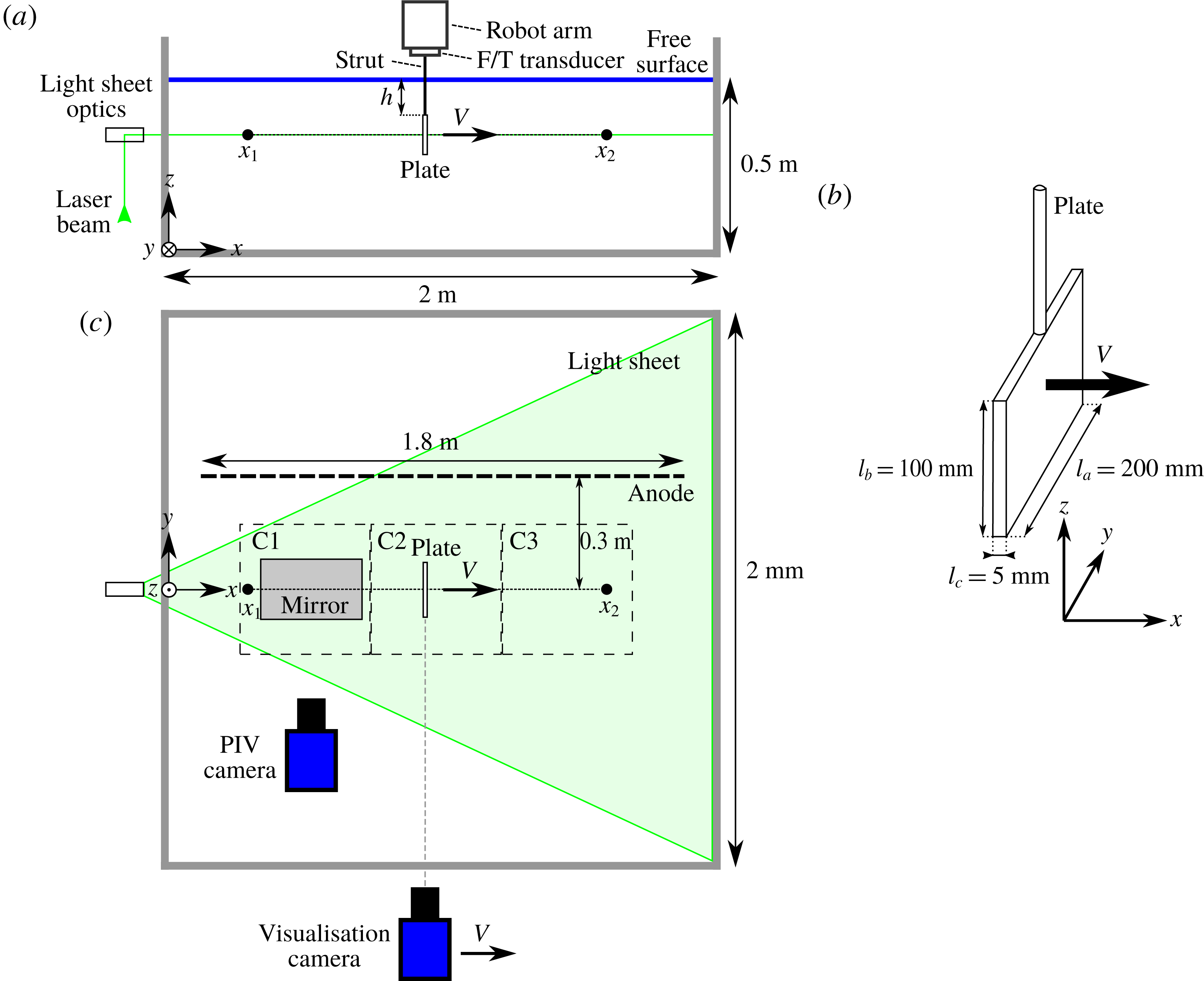
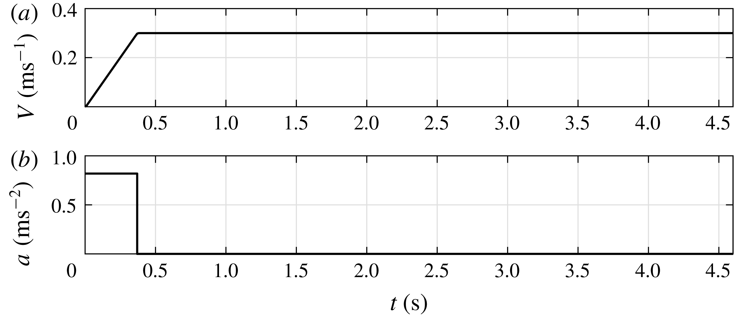
Plate velocity $V$
(a) and plate acceleration
$V$
(a) and plate acceleration $a$
(b) as a function of time
$a$
(b) as a function of time $t$
.
$t$
.
1.3 Previous work on accelerating plates
Obviously, we are not the first to investigate drag on a flat plate. Already at the beginning of the previous century Ludwig Prandtl observed the behaviour of a flow perpendicular to a plate normal to that flow in his work which translates as ‘Motion of fluids with very little viscosity’ (Prandtl Reference Prandtl1904). In the work of Hoerner (Reference Hoerner1965) an overview of the research up to 1954 on the drag of plates normal to a steady flow is found. For an accelerating motion, or flow depending on the frame of reference, we expect an increase in drag on the plate due to added mass. Although the term added mass, or alternatively hydrodynamic mass, is a common enough term in fluid mechanics, little research has been done on added mass for accelerating plates. For sufficiently small motions from rest the added mass effect can be captured by a single coefficient which is fully defined by the plate geometry (Yu Reference Yu1945; Patton Reference Patton1965; Payne Reference Payne1981).
The flow around and the drag on a uniformly accelerating plate during larger motions has been of interest since the second half of the previous century of which Koumoutsakos & Shiels (Reference Koumoutsakos and Shiels1996) provide a clear and concise summary of both numerical and experimental work carried out. It is evident that a plate uniformly accelerated from rest produces a vortex as was readily observed by Prandtl (Reference Prandtl1904). The generation of this vortex has four stages, as defined by Luchini & Tognaccini (Reference Luchini and Tognaccini2002). During the first three stages, i.e. the Rayleigh stage, viscous stage and the self-similar inviscid stage, a vortex is formed and starts growing, but remains attached to the body on which it is formed and is independent of geometry. Only during the last stage, during the vortex expulsion, the vortex starts lagging behind the body. Most experimental work and numerical work is limited in Reynolds number, $Re\approx O(10^{3})$
, or is on the very early stages of an accelerating plate, i.e. the first three stages of vortex formation. However, the first three stages already occur within a small motion of the plate, i.e. within a travelled distance of 0.5–1 times the plate height (Xu & Nitsche Reference Xu and Nitsche2015). Each of our experiments runs far into the fourth phase, which has not been investigated in great detail.
$Re\approx O(10^{3})$
, or is on the very early stages of an accelerating plate, i.e. the first three stages of vortex formation. However, the first three stages already occur within a small motion of the plate, i.e. within a travelled distance of 0.5–1 times the plate height (Xu & Nitsche Reference Xu and Nitsche2015). Each of our experiments runs far into the fourth phase, which has not been investigated in great detail.
In the work of Koumoutsakos & Shiels (Reference Koumoutsakos and Shiels1996) numerical simulations of an accelerating plate in two-dimensional viscous flow were performed up to $Re=1000$
. It was found that for a uniformly accelerated plate a Kelvin–Helmholtz-type instability was induced in the separating shear layer, which appears to be intrinsic behaviour of the flow. Previously, when this behaviour was observed during experiments by Lian & Huang (Reference Lian and Huang1989), the same observed flow behaviour was attributed to experimental defects. However, this behaviour being intrinsic to the flow was later disputed once again by Xu & Nitsche (Reference Xu and Nitsche2015), as they showed that by increasing the simulation resolution the instabilities disappear. However, Schneider et al. (Reference Schneider, Paget-Goy, Verga and Farge2014) report that the instabilities are affected by the shape of the plate tip which suggests that they are intrinsic to the flow.
$Re=1000$
. It was found that for a uniformly accelerated plate a Kelvin–Helmholtz-type instability was induced in the separating shear layer, which appears to be intrinsic behaviour of the flow. Previously, when this behaviour was observed during experiments by Lian & Huang (Reference Lian and Huang1989), the same observed flow behaviour was attributed to experimental defects. However, this behaviour being intrinsic to the flow was later disputed once again by Xu & Nitsche (Reference Xu and Nitsche2015), as they showed that by increasing the simulation resolution the instabilities disappear. However, Schneider et al. (Reference Schneider, Paget-Goy, Verga and Farge2014) report that the instabilities are affected by the shape of the plate tip which suggests that they are intrinsic to the flow.
Koumoutsakos & Shiels (Reference Koumoutsakos and Shiels1996) also found that the scaled drag coefficient collapsed onto a single curve in dimensionless time $t^{\ast }$
defined as
$t^{\ast }$
defined as $t^{\ast }=at^{2}/l_{b}$
with acceleration
$t^{\ast }=at^{2}/l_{b}$
with acceleration $a$
, dimensional time
$a$
, dimensional time $t$
and plate height
$t$
and plate height $l_{b}$
. The dimensionless time
$l_{b}$
. The dimensionless time $t^{\ast }$
is essentially the number of plate heights travelled by the plate. A similar notation was adopted by Xu & Nitsche (Reference Xu and Nitsche2015) who reported that it was more suitable to compare results with different accelerations at the same distances travelled than identical times travelled. Gharib, Rambod & Shariff (Reference Gharib, Rambod and Shariff1998) called this dimensionless time the formation time where it proved to be a universal time scale for the generation of a vortex ring by a piston. Also Ringuette, Milano & Gharib (Reference Ringuette, Milano and Gharib2007) used the formation time
$t^{\ast }$
is essentially the number of plate heights travelled by the plate. A similar notation was adopted by Xu & Nitsche (Reference Xu and Nitsche2015) who reported that it was more suitable to compare results with different accelerations at the same distances travelled than identical times travelled. Gharib, Rambod & Shariff (Reference Gharib, Rambod and Shariff1998) called this dimensionless time the formation time where it proved to be a universal time scale for the generation of a vortex ring by a piston. Also Ringuette, Milano & Gharib (Reference Ringuette, Milano and Gharib2007) used the formation time $t^{\ast }$
to identify vortex shedding events at the edges of a uniformly accelerated semi-infinite plate normal to the flow. Also in this study the formation time appears to be a useful scaling parameter with respect to vortex shedding. Throughout this study, parameters and variables are expressed in their dimensional form unless their dimensionless counterpart proves a valuable addition to the analysis, i.e. some universal scaling becomes apparent by their use.
$t^{\ast }$
to identify vortex shedding events at the edges of a uniformly accelerated semi-infinite plate normal to the flow. Also in this study the formation time appears to be a useful scaling parameter with respect to vortex shedding. Throughout this study, parameters and variables are expressed in their dimensional form unless their dimensionless counterpart proves a valuable addition to the analysis, i.e. some universal scaling becomes apparent by their use.
The experiment carried out by Ringuette et al. (Reference Ringuette, Milano and Gharib2007) somewhat resembles our experiment. The main difference is that our plate is not semi-infinite but three-dimensional, and our plate is not piercing the surface but is submerged below the surface. Also the Reynolds number in our experiments are an order of magnitude larger, i.e. $O(10^{4})$
versus
$O(10^{4})$
versus $O(10^{3})$
. In their work, force measurements are combined with visualisation techniques and quantitative flow measurements by means of particle image velocimetry (PIV). The latter is used to obtain the vorticity in the flow and from there the dimensionless circulation which can be used to identify vortex shedding events. In this study we use similar techniques to investigate the flow around the plate.
$O(10^{3})$
. In their work, force measurements are combined with visualisation techniques and quantitative flow measurements by means of particle image velocimetry (PIV). The latter is used to obtain the vorticity in the flow and from there the dimensionless circulation which can be used to identify vortex shedding events. In this study we use similar techniques to investigate the flow around the plate.
2 Experimental set-up
Figure 1 shows the experimental set-up used in this study. All experiments are done in an open-top glass tank with a horizontal cross-section of $2~\text{m}\times 2~\text{m}$
and a height of 0.6 m. The dimensions of the tank are chosen to be as large as practically possible to avoid blockage effects and wall effects. The tank is filled with water up to a level of 0.5 m to avoid spilling over the edge of the tank. The flat plate used in this study has a width
$2~\text{m}\times 2~\text{m}$
and a height of 0.6 m. The dimensions of the tank are chosen to be as large as practically possible to avoid blockage effects and wall effects. The tank is filled with water up to a level of 0.5 m to avoid spilling over the edge of the tank. The flat plate used in this study has a width $l_{a}=200$
mm and a height
$l_{a}=200$
mm and a height $l_{b}=100$
mm which results in a surface blockage ratio of 0.02, i.e. the ratio of the plate area (
$l_{b}=100$
mm which results in a surface blockage ratio of 0.02, i.e. the ratio of the plate area ( $0.2~\text{m}\times 0.1~\text{m}$
) over the tank cross-section perpendicular to the direction of motion of the plate (
$0.2~\text{m}\times 0.1~\text{m}$
) over the tank cross-section perpendicular to the direction of motion of the plate ( $2~\text{m}\times 0.5~\text{m}$
). According to literature, e.g. West & Apelt (Reference West and Apelt1982), at this ratio the presence of the walls of the tank do not have a significant effect on the drag. To match the rowing oar blade on a 1 : 2 scale the plate thickness
$2~\text{m}\times 0.5~\text{m}$
). According to literature, e.g. West & Apelt (Reference West and Apelt1982), at this ratio the presence of the walls of the tank do not have a significant effect on the drag. To match the rowing oar blade on a 1 : 2 scale the plate thickness $l_{c}$
should be 2.5 mm. However, to avoid flapping or flexing of the plate a compromise was reached at a plate thickness
$l_{c}$
should be 2.5 mm. However, to avoid flapping or flexing of the plate a compromise was reached at a plate thickness $l_{c}=4$
mm. The plate is aligned such that its major dimensions
$l_{c}=4$
mm. The plate is aligned such that its major dimensions $l_{a}$
and
$l_{a}$
and $l_{b}$
are parallel to the
$l_{b}$
are parallel to the $y$
and
$y$
and $z$
direction, respectively, see figure 1(b). The plate is mounted to an industrial robot arm (Reis Robotics RL50) with a streamlined strut piercing the air–water interface. A force/torque transducer (F/T transducer) is installed between the robot arm and the strut to measure the hydrodynamic forces acting on the plate. The hydrodynamic forces on the streamlined strut are considered to be negligible compared to those on the flat plate.
$z$
direction, respectively, see figure 1(b). The plate is mounted to an industrial robot arm (Reis Robotics RL50) with a streamlined strut piercing the air–water interface. A force/torque transducer (F/T transducer) is installed between the robot arm and the strut to measure the hydrodynamic forces acting on the plate. The hydrodynamic forces on the streamlined strut are considered to be negligible compared to those on the flat plate.
2.1 Kinematics
The robot moves the flat plate along a straight line in the $x$
-direction, from
$x$
-direction, from $x_{1}$
to
$x_{1}$
to $x_{2}$
, over a distance of 1.4 m (figure 1), starting and stopping at a distance of three times the plate height
$x_{2}$
, over a distance of 1.4 m (figure 1), starting and stopping at a distance of three times the plate height $l_{b}$
from the walls, such that the walls do not affect the flow around the plate. The velocity fields obtained from the PIV measurements show that the flow is unperturbed, i.e. a flow velocity magnitude
$l_{b}$
from the walls, such that the walls do not affect the flow around the plate. The velocity fields obtained from the PIV measurements show that the flow is unperturbed, i.e. a flow velocity magnitude ${<}1\,\%$
of the plate velocity
${<}1\,\%$
of the plate velocity $V$
, at 2.4 plate heights
$V$
, at 2.4 plate heights $l_{b}$
ahead of the plate. To investigate the effect of the free surface on the drag, the immersion depth
$l_{b}$
ahead of the plate. To investigate the effect of the free surface on the drag, the immersion depth $h$
, defined as the distance between the top edge of the plate and the water surface, as shown in figure 1, is varied from 0 to 200 mm. The plate is linearly accelerated to a velocity
$h$
, defined as the distance between the top edge of the plate and the water surface, as shown in figure 1, is varied from 0 to 200 mm. The plate is linearly accelerated to a velocity $V=0.30~\text{m}~\text{s}^{-1}$
; see figure 2. The acceleration of the robot is set to
$V=0.30~\text{m}~\text{s}^{-1}$
; see figure 2. The acceleration of the robot is set to $a=0.82~\text{m}~\text{s}^{-2}$
so that the prescribed velocity of
$a=0.82~\text{m}~\text{s}^{-2}$
so that the prescribed velocity of $V=0.30~\text{m}~\text{s}^{-1}$
is reached in 0.36 s. At
$V=0.30~\text{m}~\text{s}^{-1}$
is reached in 0.36 s. At $V=0.30~\text{m}~\text{s}^{-1}$
the Reynolds number (using the plate width
$V=0.30~\text{m}~\text{s}^{-1}$
the Reynolds number (using the plate width $l_{a}$
as a characteristic length) is
$l_{a}$
as a characteristic length) is $Re=60\times 10^{3}$
, which is well into the turbulent regime. Higher velocities would complicate the experiments by increasing the settling time of the turbid water in the tank between experiments, and would increase the risk of splashing and spills. During the experiments only very small capillary waves are observed, which hold very little energy. Due to the absence of waves we expect a small Froude number, which is defined as
$Re=60\times 10^{3}$
, which is well into the turbulent regime. Higher velocities would complicate the experiments by increasing the settling time of the turbid water in the tank between experiments, and would increase the risk of splashing and spills. During the experiments only very small capillary waves are observed, which hold very little energy. Due to the absence of waves we expect a small Froude number, which is defined as
 $$\begin{eqnarray}Fr=\frac{V}{\sqrt{gL}},\end{eqnarray}$$
where $g$
is the gravitational acceleration, and
$g$
is the gravitational acceleration, and $L$
is a representative length scale. However, it is hard to define a representative length scale in the geometry and/or water depth used in this experiment. Instead of arbitrarily choosing a length scale we reason that a critical Froude number
$L$
is a representative length scale. However, it is hard to define a representative length scale in the geometry and/or water depth used in this experiment. Instead of arbitrarily choosing a length scale we reason that a critical Froude number $Fr=1$
is reached at a critical length scale
$Fr=1$
is reached at a critical length scale $L_{crit}=V^{2}/g=0.30^{2}/9.81=0.009$
m. Since the relevant major length scales in this experiment, e.g. the major plate dimensions or the tank depth, are much larger than this critical length scale, such that
$L_{crit}=V^{2}/g=0.30^{2}/9.81=0.009$
m. Since the relevant major length scales in this experiment, e.g. the major plate dimensions or the tank depth, are much larger than this critical length scale, such that $Fr\ll 1$
.
$Fr\ll 1$
.
2.2 Force and path data acquisition
The robot itself provides the data on the position $x(t)$
and the velocity
$x(t)$
and the velocity $V(t)$
at a default rate of 92 Hz. The robot position data are within 0.1 mm repeatable, with a resolution of
$V(t)$
at a default rate of 92 Hz. The robot position data are within 0.1 mm repeatable, with a resolution of $1~\unicode[STIX]{x03BC}\text{m}$
. To analyse the forces on the flat plate a force (AMTI 6-DOF) is used that measures the force at a rate of 10 kHz.
$1~\unicode[STIX]{x03BC}\text{m}$
. To analyse the forces on the flat plate a force (AMTI 6-DOF) is used that measures the force at a rate of 10 kHz.
2.3 Hydrogen bubble flow visualisation
To visualise the flow we use hydrogen bubble flow visualisation. Installed on the front face of the plate (facing the positive $x$
-direction) is a 0.6 mm thick copper wire mesh that acts as the cathode. A 1.8 m long stainless steel screen that is placed parallel to the plate path at a distance of 0.6 m acts as the anode, see figure 1. Using an electric potential of 30 V hydrogen bubbles are created at the front surface of the plate. To increase the bubble production rate to a level suitable for visualisation the conductivity of the water was increased by adding 2.5 kg of sodium sulphate. The hydrogen bubbles were illuminated through the glass bottom of the tank using flood lights (
$x$
-direction) is a 0.6 mm thick copper wire mesh that acts as the cathode. A 1.8 m long stainless steel screen that is placed parallel to the plate path at a distance of 0.6 m acts as the anode, see figure 1. Using an electric potential of 30 V hydrogen bubbles are created at the front surface of the plate. To increase the bubble production rate to a level suitable for visualisation the conductivity of the water was increased by adding 2.5 kg of sodium sulphate. The hydrogen bubbles were illuminated through the glass bottom of the tank using flood lights ( $3\times 400$
W). Images of the hydrogen bubbles were taken with a high-speed camera (Phantom VEO 640L with a 105 mm Nikon lens) at a frame rate of 500 frames per second (f.p.s.). During the recording the camera moved (manually) with the plate in the positive
$3\times 400$
W). Images of the hydrogen bubbles were taken with a high-speed camera (Phantom VEO 640L with a 105 mm Nikon lens) at a frame rate of 500 frames per second (f.p.s.). During the recording the camera moved (manually) with the plate in the positive $x$
-direction such that the plate and its wake remained in the camera’s field of view.
$x$
-direction such that the plate and its wake remained in the camera’s field of view.
2.4 Particle image velocimetry
To quantify the flow field we used planar particle image velocimetry (PIV). The field of view is in the horizontal $x$
,
$x$
, $y$
-plane through the centre of the plate. A 4 megapixel high-speed camera (LaVision Imager Pro HS) was used to capture the flow through the glass bottom upwards in the positive
$y$
-plane through the centre of the plate. A 4 megapixel high-speed camera (LaVision Imager Pro HS) was used to capture the flow through the glass bottom upwards in the positive $z$
-direction at a frame rate of 1000 f.p.s. To capture the entire run of the plate over 1.4 m we captured the flow at three different locations along the
$z$
-direction at a frame rate of 1000 f.p.s. To capture the entire run of the plate over 1.4 m we captured the flow at three different locations along the $x$
-axis, each time using a field of view of approximately
$x$
-axis, each time using a field of view of approximately $0.6~\text{m}\times 0.6~\text{m}$
, and these were stitched together to cover the entire run, as shown in figure 1. Neutrally buoyant fluorescent spherical tracer particles (Cospheric UVPMS-BR-0.995, 53–
$0.6~\text{m}\times 0.6~\text{m}$
, and these were stitched together to cover the entire run, as shown in figure 1. Neutrally buoyant fluorescent spherical tracer particles (Cospheric UVPMS-BR-0.995, 53– $63~\unicode[STIX]{x03BC}\text{m}$
diameter) were added to the flow (10 g) and were illuminated using a 532 nm Nd-YAG 150 W laser (Litron LDY304-PIV). The acquired images were analysed using commercial software (LaVision DaVis 8.4). To create image pairs from the sequential images acquired at 1000 f.p.s. every
$63~\unicode[STIX]{x03BC}\text{m}$
diameter) were added to the flow (10 g) and were illuminated using a 532 nm Nd-YAG 150 W laser (Litron LDY304-PIV). The acquired images were analysed using commercial software (LaVision DaVis 8.4). To create image pairs from the sequential images acquired at 1000 f.p.s. every $n$
th frame was paired with the (
$n$
th frame was paired with the ( $n+6$
)th frame resulting in a 6 ms exposure time delay
$n+6$
)th frame resulting in a 6 ms exposure time delay $\unicode[STIX]{x0394}t$
to ensure sufficient displacement of the particle images in the region of interest, i.e. the wake behind the plate. A multi-pass correlation based PIV algorithm was used to obtain the flow velocity field from the image pairs. The interrogation windows of the three subsequent passes were
$\unicode[STIX]{x0394}t$
to ensure sufficient displacement of the particle images in the region of interest, i.e. the wake behind the plate. A multi-pass correlation based PIV algorithm was used to obtain the flow velocity field from the image pairs. The interrogation windows of the three subsequent passes were $48\times 48$
pixels for the first pass, and
$48\times 48$
pixels for the first pass, and $24\times 24$
pixels for the second and third passes. A 50 % overlap between adjacent interrogation positions was used. This resulted in velocity vector fields with a vector spacing of 3.2 mm and a cumulative first and second vector choice of
$24\times 24$
pixels for the second and third passes. A 50 % overlap between adjacent interrogation positions was used. This resulted in velocity vector fields with a vector spacing of 3.2 mm and a cumulative first and second vector choice of ${>}98\,\%$
in the area of interest, i.e. in the wake of the plate.
${>}98\,\%$
in the area of interest, i.e. in the wake of the plate.
3 Results
3.1 Typical result from the force measurements
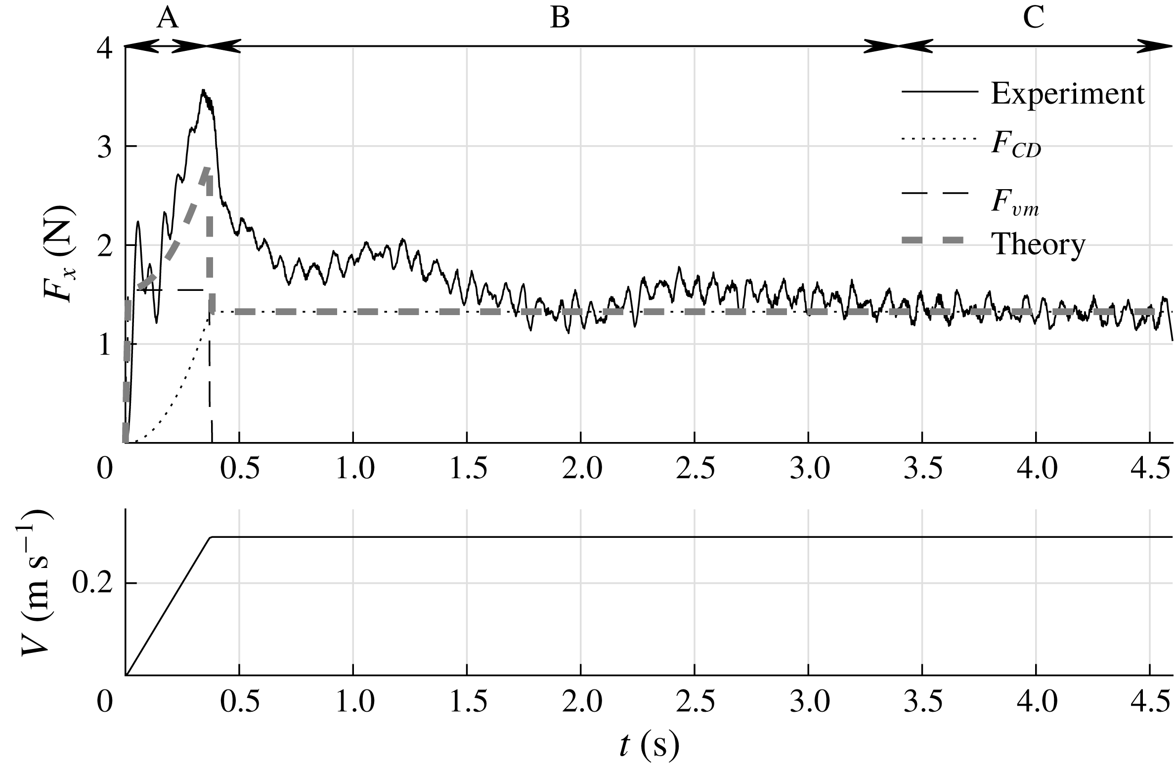
During each run the instantaneous force $F_{x}$
(perpendicular to the plate surface) is sampled at a rate of 10 kHz. The grey line in figure 3 represents
$F_{x}$
(perpendicular to the plate surface) is sampled at a rate of 10 kHz. The grey line in figure 3 represents $F_{x}$
as a function of time for an experiment with a velocity
$F_{x}$
as a function of time for an experiment with a velocity $V=0.30~\text{m}~\text{s}^{-1}$
, a plate depth of
$V=0.30~\text{m}~\text{s}^{-1}$
, a plate depth of $h=100$
mm and an acceleration of
$h=100$
mm and an acceleration of $a=0.82~\text{m}~\text{s}^{-2}$
. As one can see, the 10 kHz sampled raw signal shows significant fluctuations. All calculations and analyses are performed using the unfiltered signals. However, for better readability the signal is filtered using a second-order Savitzky–Golay filter (Savitzky & Golay Reference Savitzky and Golay1964) with a filter width of 201 samples, i.e. 0.02 s. The black line in figure 3 represents the filtered signal. The force signal exhibits a clear initial peak at 0.36 s which coincides with the time when the plate reaches its maximum velocity of
$a=0.82~\text{m}~\text{s}^{-2}$
. As one can see, the 10 kHz sampled raw signal shows significant fluctuations. All calculations and analyses are performed using the unfiltered signals. However, for better readability the signal is filtered using a second-order Savitzky–Golay filter (Savitzky & Golay Reference Savitzky and Golay1964) with a filter width of 201 samples, i.e. 0.02 s. The black line in figure 3 represents the filtered signal. The force signal exhibits a clear initial peak at 0.36 s which coincides with the time when the plate reaches its maximum velocity of $V=0.30~\text{m}~\text{s}^{-1}$
; see figure 3(b). The initial peak is due to the added mass and the acceleration of the plate, as is discussed in detail in § 3.7. The time interval
$V=0.30~\text{m}~\text{s}^{-1}$
; see figure 3(b). The initial peak is due to the added mass and the acceleration of the plate, as is discussed in detail in § 3.7. The time interval $0<t<0.36$
s is called the ‘acceleration phase’ and is indicated by A in figure 3. After the peak, the force gradually decreases and finally reaches a steady value for
$0<t<0.36$
s is called the ‘acceleration phase’ and is indicated by A in figure 3. After the peak, the force gradually decreases and finally reaches a steady value for $t\gtrsim 3.4$
s. This phase is called the ‘steady phase’ and is indicated by C. The time interval in between the initial peak and the beginning of the steady phase (
$t\gtrsim 3.4$
s. This phase is called the ‘steady phase’ and is indicated by C. The time interval in between the initial peak and the beginning of the steady phase ( $0.36~\text{s}<t<3.4$
s) is called the ‘transition phase’ and is indicated by B. The measurement ends at
$0.36~\text{s}<t<3.4$
s) is called the ‘transition phase’ and is indicated by B. The measurement ends at $t=4.6$
s. It is noted that the force signal shows two distinct local maxima during the transition phase B, indicated as ‘peak 1’ and ‘peak 2’ in figure 3. In § 3.6 it is shown that these peaks are related to the development of large flow structures in the wake of the plate. Also, throughout the experiment, high-frequency oscillations are present in the force signal, which is due to Kelvin–Helmholtz-like instabilities in the shear layer, which is further discussed in § 3.4. Right after starting the plate we observe a local peak followed by a dip in the force signal, i.e. a step response as indicated in figure 3. This is a result of the finite stiffness of the plate, the force transducer and the streamlined strut that connects the two. This finite stiffness causes a typical response of a mass–spring–damper system to a step function; in this case the sudden acceleration of the plate causes a sudden force due to the hydrodynamic mass and mass of the plate (Meirovitch Reference Meirovitch2001).
$t=4.6$
s. It is noted that the force signal shows two distinct local maxima during the transition phase B, indicated as ‘peak 1’ and ‘peak 2’ in figure 3. In § 3.6 it is shown that these peaks are related to the development of large flow structures in the wake of the plate. Also, throughout the experiment, high-frequency oscillations are present in the force signal, which is due to Kelvin–Helmholtz-like instabilities in the shear layer, which is further discussed in § 3.4. Right after starting the plate we observe a local peak followed by a dip in the force signal, i.e. a step response as indicated in figure 3. This is a result of the finite stiffness of the plate, the force transducer and the streamlined strut that connects the two. This finite stiffness causes a typical response of a mass–spring–damper system to a step function; in this case the sudden acceleration of the plate causes a sudden force due to the hydrodynamic mass and mass of the plate (Meirovitch Reference Meirovitch2001).
(a) A typical unfiltered force signal $F_{x}$
sampled at 10 kHz (grey) and the filtered force signal (black). Throughout the force signal high-frequency oscillations are present which are caused by Kelvin–Helmholtz-like instabilities in the shear layer as discussed in § 3.4. Right after starting the plate we observe a step response due to the finite stiffness of the plate, force transducer and the strut which connects the two. (b) The plate velocity
$F_{x}$
sampled at 10 kHz (grey) and the filtered force signal (black). Throughout the force signal high-frequency oscillations are present which are caused by Kelvin–Helmholtz-like instabilities in the shear layer as discussed in § 3.4. Right after starting the plate we observe a step response due to the finite stiffness of the plate, force transducer and the strut which connects the two. (b) The plate velocity $V$
as a function of time.
$V$
as a function of time.

3.2 The effect of the plate depth on the steady-phase drag
The plate is moved through the tank for different immersion depths $h$
to investigate the effect of the free surface on the drag on the plate. The immersion depth
$h$
to investigate the effect of the free surface on the drag on the plate. The immersion depth $h$
is varied between 0 and 200 mm in a randomised order. In total 140 runs were carried out.
$h$
is varied between 0 and 200 mm in a randomised order. In total 140 runs were carried out.
The drag force $F_{x}$
during the steady phase is expressed as
$F_{x}$
during the steady phase is expressed as
 $$\begin{eqnarray}F_{x}={\textstyle \frac{1}{2}}\unicode[STIX]{x1D70C}V^{2}C_{D}A,\end{eqnarray}$$
where $\unicode[STIX]{x1D70C}$
is the fluid density,
$\unicode[STIX]{x1D70C}$
is the fluid density, $V$
the plate velocity,
$V$
the plate velocity, $A$
the frontal area of the plate and
$A$
the frontal area of the plate and $C_{D}$
the steady-phase drag coefficient. For each run the steady-phase drag coefficient
$C_{D}$
the steady-phase drag coefficient. For each run the steady-phase drag coefficient $C_{D}$
is calculated and plotted in figure 4 using open markers, where each marker represents
$C_{D}$
is calculated and plotted in figure 4 using open markers, where each marker represents $C_{D}$
of a single run at a given depth
$C_{D}$
of a single run at a given depth $h$
. The steady phase drag coefficient
$h$
. The steady phase drag coefficient $C_{D}$
reaches a minimum value of
$C_{D}$
reaches a minimum value of $C_{D}=1.10$
for
$C_{D}=1.10$
for $h=0$
, i.e. when the top of the plate is at the surface. For larger values of
$h=0$
, i.e. when the top of the plate is at the surface. For larger values of $h$
, i.e. when the plate is submerged, the drag coefficient increases to a peak value of
$h$
, i.e. when the plate is submerged, the drag coefficient increases to a peak value of $C_{D}=1.60$
at a depth
$C_{D}=1.60$
at a depth $h=20$
mm; a relative increase of 45 %. When the plate is submerged further below the surface the drag coefficient decreases, and a constant value of
$h=20$
mm; a relative increase of 45 %. When the plate is submerged further below the surface the drag coefficient decreases, and a constant value of $C_{D}=1.3$
is reached for large
$C_{D}=1.3$
is reached for large $h$
.
$h$
.
The steady-phase drag coefficient $C_{D}$
as function of plate depth
$C_{D}$
as function of plate depth $h$
. For reference the dashed line gives the
$h$
. For reference the dashed line gives the $C_{D}$
value for flow over a fence (
$C_{D}$
value for flow over a fence ( $C_{D}=1.10$
) and the solid line the
$C_{D}=1.10$
) and the solid line the $C_{D}$
value for flow around a 1 : 2 aspect ratio plate (
$C_{D}$
value for flow around a 1 : 2 aspect ratio plate ( $C_{D}=1.30$
).
$C_{D}=1.30$
).

To the knowledge of the authors, the observed behaviour of $C_{D}$
with respect to the plate depth
$C_{D}$
with respect to the plate depth $h$
has not been reported previously. However, to be able to make a comparison with the literature we consider two limiting cases. The first limiting case occurs for large
$h$
has not been reported previously. However, to be able to make a comparison with the literature we consider two limiting cases. The first limiting case occurs for large $h$
where the free surface does not affect the drag on the plate any more. For the deep water cases we found
$h$
where the free surface does not affect the drag on the plate any more. For the deep water cases we found $C_{D}=1.30$
, which is in close agreement with a value of
$C_{D}=1.30$
, which is in close agreement with a value of $C_{D}=1.26$
–1.32 for a fully submerged plate with
$C_{D}=1.26$
–1.32 for a fully submerged plate with $AR=6$
(Schubauer & Dryden Reference Schubauer and Dryden1937) and
$AR=6$
(Schubauer & Dryden Reference Schubauer and Dryden1937) and $C_{D}=1.2$
–1.26 for square plates (Bearman Reference Bearman1971). Another limiting case occurs for
$C_{D}=1.2$
–1.26 for square plates (Bearman Reference Bearman1971). Another limiting case occurs for $h=0$
mm, where we compare the measured drag coefficient with that of a fence, as if the free surface acts as a wall such that the flow does not pass over the top of the plate. Again the found drag coefficient
$h=0$
mm, where we compare the measured drag coefficient with that of a fence, as if the free surface acts as a wall such that the flow does not pass over the top of the plate. Again the found drag coefficient $C_{D}=1.10$
matches well with values found in the literature
$C_{D}=1.10$
matches well with values found in the literature $C_{D}=1.05$
–1.12 (Jacobs Reference Jacobs1985). The assumption that the plate acts like a fence is verified by letting the plate pierce the surface such that no water flows over the plate, i.e.
$C_{D}=1.05$
–1.12 (Jacobs Reference Jacobs1985). The assumption that the plate acts like a fence is verified by letting the plate pierce the surface such that no water flows over the plate, i.e. $h<0$
. The drag coefficients for a partially submerged plate are represented by the closed markers in figure 4. Of course, for this surface piercing case the frontal projected area of submerged part of the plate is used for calculating
$h<0$
. The drag coefficients for a partially submerged plate are represented by the closed markers in figure 4. Of course, for this surface piercing case the frontal projected area of submerged part of the plate is used for calculating $C_{D}$
.
$C_{D}$
.
3.3 Instantaneous force signals for selected depths
Three cases are selected for further analysis: the surface case $h=0$
mm, the maximum drag case
$h=0$
mm, the maximum drag case $h=20$
mm and the case
$h=20$
mm and the case $h=100$
mm, which equals one blade height
$h=100$
mm, which equals one blade height $l_{b}$
. The surface case (
$l_{b}$
. The surface case ( $h=0$
mm) corresponds to the neutrally buoyant position of an actual rowing oar blade,
$h=0$
mm) corresponds to the neutrally buoyant position of an actual rowing oar blade, $h=100$
mm, i.e. one blade height, is the practical limit of immersion during actual rowing, and the maximum drag case (
$h=100$
mm, i.e. one blade height, is the practical limit of immersion during actual rowing, and the maximum drag case ( $h=20$
mm) would be optimal for propulsion. Note that a local minimum and trend break can be seen at
$h=20$
mm) would be optimal for propulsion. Note that a local minimum and trend break can be seen at $h=50$
mm. Although not investigated in this study, we speculate that two drag enhancing mechanisms play a role at this depth as further discussed in § 3.6. The flow visualisations in § 3.5 show that the case of
$h=50$
mm. Although not investigated in this study, we speculate that two drag enhancing mechanisms play a role at this depth as further discussed in § 3.6. The flow visualisations in § 3.5 show that the case of $h=100$
mm develops a symmetric wake (top–bottom) which suggests it may also be representative for a fully submerged plate. The three cases are indicated in figure 4. For the three selected depths, i.e.
$h=100$
mm develops a symmetric wake (top–bottom) which suggests it may also be representative for a fully submerged plate. The three cases are indicated in figure 4. For the three selected depths, i.e. $h=0$
mm,
$h=0$
mm, $h=20$
mm and
$h=20$
mm and $h=100$
mm, experiments are carried out at a velocity
$h=100$
mm, experiments are carried out at a velocity $V=0.30~\text{m}~\text{s}^{-1}$
and an acceleration
$V=0.30~\text{m}~\text{s}^{-1}$
and an acceleration $a=0.82~\text{m}~\text{s}^{-2}$
. The instantaneous drag force profiles for these three cases are shown in figure 5. It is observed that for all three cases the plate drag is rapidly increasing during the acceleration phase (A), and the maximum drag is reached at the end of this phase. For the case
$a=0.82~\text{m}~\text{s}^{-2}$
. The instantaneous drag force profiles for these three cases are shown in figure 5. It is observed that for all three cases the plate drag is rapidly increasing during the acceleration phase (A), and the maximum drag is reached at the end of this phase. For the case $h=0$
mm, the drag force is significantly lower during most of the transition phase (B) and during the steady phase (C). For the case
$h=0$
mm, the drag force is significantly lower during most of the transition phase (B) and during the steady phase (C). For the case $h=20$
mm the drag is higher than in the other cases for
$h=20$
mm the drag is higher than in the other cases for $t>1.5$
s, which also follows from figure 4. Significant differences occur during the transition phase. The force signals show a very different decay to their steady-phase values. The case
$t>1.5$
s, which also follows from figure 4. Significant differences occur during the transition phase. The force signals show a very different decay to their steady-phase values. The case $h=0$
mm initially shows the slowest decay but reaches the lowest steady state drag value, while the case
$h=0$
mm initially shows the slowest decay but reaches the lowest steady state drag value, while the case $h=100$
mm shows the fastest decay but eventually reaches a relatively high steady-phase drag value. Also, the peaks 1 and 2 are only present during the transition phase (B) of the case
$h=100$
mm shows the fastest decay but eventually reaches a relatively high steady-phase drag value. Also, the peaks 1 and 2 are only present during the transition phase (B) of the case $h=100$
mm.
$h=100$
mm.
The drag force signals $F_{x}(t)$
for the three selected plate depths,
$F_{x}(t)$
for the three selected plate depths, $h=0$
mm,
$h=0$
mm, $h=20$
mm and
$h=20$
mm and $h=100$
mm. The vertical dashed lines indicate time instances
$h=100$
mm. The vertical dashed lines indicate time instances $t_{1}$
,
$t_{1}$
, $t_{2}$
and
$t_{2}$
and $t_{3}$
when snapshots of the hydrogen bubble flow visualisation were taken as discussed in § 3.5.
$t_{3}$
when snapshots of the hydrogen bubble flow visualisation were taken as discussed in § 3.5.
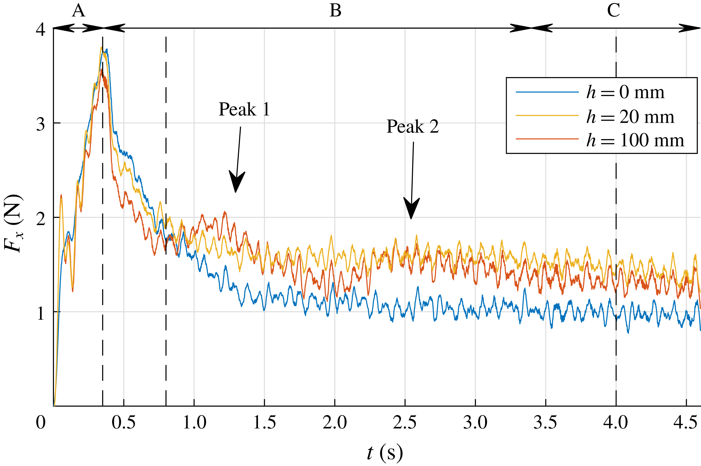
The drag signals for the three selected cases all show a steep increase during the acceleration phase and a relatively gradual decrease during the transition phase towards the steady phase. Traditionally, the steady-phase drag force is described by (3.1). However, when dealing with an accelerating object in a quiescent fluid the effect of the added mass must be incorporated into the description of the drag force $F_{x}$
:
$F_{x}$
:
 $$\begin{eqnarray}F_{x}(t)=F_{CD}(t)+F_{vm}(t)=\underbrace{{\textstyle \frac{1}{2}}\unicode[STIX]{x1D70C}V(t)^{2}C_{D}A}_{F_{CD}(t)}+\underbrace{\overbrace{(m_{p}+m_{h})}^{m_{v}}a(t)}_{F_{vm}(t)},\end{eqnarray}$$
where $F_{CD}$
is the steady-phase drag force and
$F_{CD}$
is the steady-phase drag force and $F_{vm}$
the product of the virtual mass
$F_{vm}$
the product of the virtual mass $m_{v}$
and the plate acceleration
$m_{v}$
and the plate acceleration $a$
. The virtual mass
$a$
. The virtual mass $m_{v}$
is the sum of the plate mass
$m_{v}$
is the sum of the plate mass $m_{p}$
and the hydrodynamic mass
$m_{p}$
and the hydrodynamic mass $m_{h}$
. All variables in (3.2) are known except for the hydrodynamic mass
$m_{h}$
. All variables in (3.2) are known except for the hydrodynamic mass $m_{h}$
. The plate velocity
$m_{h}$
. The plate velocity $V(t)$
and the plate acceleration
$V(t)$
and the plate acceleration $a$
are prescribed as previously shown in figure 2. For each run the value for
$a$
are prescribed as previously shown in figure 2. For each run the value for $C_{D}$
is taken from figure 4. The plate mass
$C_{D}$
is taken from figure 4. The plate mass $m_{p}=0.400$
kg, while the hydrodynamic mass
$m_{p}=0.400$
kg, while the hydrodynamic mass $m_{h}$
for a submerged geometry accelerating from rest is estimated by using an empirical correlation. For a rectangular flat plate with an aspect ratio of
$m_{h}$
for a submerged geometry accelerating from rest is estimated by using an empirical correlation. For a rectangular flat plate with an aspect ratio of $AR=2$
for inviscid frictionless flow the hydrodynamic mass is modelled as (Patton Reference Patton1965):
$AR=2$
for inviscid frictionless flow the hydrodynamic mass is modelled as (Patton Reference Patton1965):
 $$\begin{eqnarray}m_{h(Patton)}=0.84\frac{\unicode[STIX]{x03C0}}{4}\unicode[STIX]{x1D70C}l_{a}l_{b}^{2}=1.3~\text{kg},\end{eqnarray}$$
where $l_{a}$
and
$l_{a}$
and $l_{b}$
are the major dimensions of the plate (with
$l_{b}$
are the major dimensions of the plate (with $l_{a}>l_{b}$
). Alternatively, Yu (Reference Yu1945) provides an empirical correlation valid for arbitrary plate aspect ratio and plate thickness
$l_{a}>l_{b}$
). Alternatively, Yu (Reference Yu1945) provides an empirical correlation valid for arbitrary plate aspect ratio and plate thickness $l_{c}$
:
$l_{c}$
:
 $$\begin{eqnarray}m_{h(Yu)}=\unicode[STIX]{x1D70C}\left[0.788\frac{l_{a}^{2}l_{b}^{2}}{(l_{a}^{2}+l_{b}^{2})^{1/2}}+0.0619l_{a}l_{b}l_{c}^{1/2}\right].\end{eqnarray}$$
Figure 6 shows the measured drag force $F_{x}(t)$
for
$F_{x}(t)$
for $h=100$
mm, next to the theoretical drag force, equation (3.2) with
$h=100$
mm, next to the theoretical drag force, equation (3.2) with $m_{h}$
according to (3.4). The predicted initial peak in drag force of 2.8 N significantly underestimates the measured peak of 3.6 N. When using expression (3.3) for the hydrodynamic mass, the initial peak is estimated to be even lower at 2.6 N. Also, the predicted force shows a sharp drop as soon as the acceleration of the plate ends at
$m_{h}$
according to (3.4). The predicted initial peak in drag force of 2.8 N significantly underestimates the measured peak of 3.6 N. When using expression (3.3) for the hydrodynamic mass, the initial peak is estimated to be even lower at 2.6 N. Also, the predicted force shows a sharp drop as soon as the acceleration of the plate ends at $t=0.36$
s. This is because a force is no longer required for accelerating the virtual mass
$t=0.36$
s. This is because a force is no longer required for accelerating the virtual mass $m_{v}$
. However, in the measurements a much more gradual decrease in drag force after the initial peak at
$m_{v}$
. However, in the measurements a much more gradual decrease in drag force after the initial peak at $t=0.36$
s is observed. During experiments, upon accelerating the plate for
$t=0.36$
s is observed. During experiments, upon accelerating the plate for $h=0$
mm and
$h=0$
mm and $h=20$
mm, a vortex pair is visible at the free surface which is a viscous effect, potentially explaining the mismatch between theory and experiment since the correlations for the hydrodynamic mass are for inviscid flow only. The formation of these vortices is further addressed in § 3.5.
$h=20$
mm, a vortex pair is visible at the free surface which is a viscous effect, potentially explaining the mismatch between theory and experiment since the correlations for the hydrodynamic mass are for inviscid flow only. The formation of these vortices is further addressed in § 3.5.


3.4 Shear layer instabilities
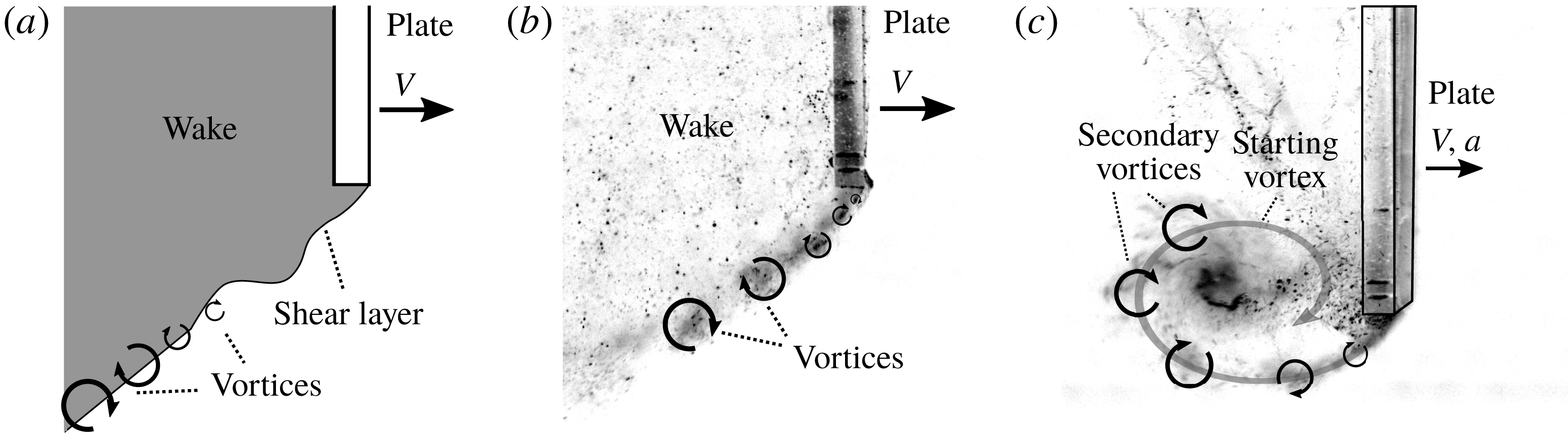
As described in the introduction, many studies investigating accelerating flat plates encounter vortices which are formed in the shear layer between the wake of the plate and the flow separating at the plate edge, e.g. Lian & Huang (Reference Lian and Huang1989). The mechanism by which these vortices are generated is similar to that of the Kelvin–Helmholtz instability and is depicted in figure 7(a). These shear layer instabilities are very close to the plate and can be seen in the force signal; see figure 3. These are also visible in the flow visualisations discussed in § 3.5, where the hydrogen bubbles end up in the vortex cores; see figure 7(c). Not only during the acceleration phase, but also during the other phases, i.e. where the plate travels at constant velocity, the secondary vortices are generated in the shear layer at a consistent frequency. When the starting vortex has disintegrated the generated secondary vortices are simply shed into the wake, as shown in figure 7(b). The frequency at which the vortices are generated was determined based on the flow visualisations for each $h$
at
$h$
at $a=0.82~\text{m}~\text{s}^{-2}$
and
$a=0.82~\text{m}~\text{s}^{-2}$
and $V=0.20^{-1}$
and
$V=0.20^{-1}$
and $0.30~\text{m}~\text{s}^{-1}$
and was found to be 17 Hz. The power spectrum of the drag force signal consistently shows a peak at this frequency for all runs. The power spectra determined for different values of acceleration, velocity and immersion depth, were all similar, i.e. the eight most dominant frequencies all lie in the range of 13–20 Hz with the most dominant frequency at approximately 17 Hz. Minor variations between runs are observed. We hypothesise that these variations are due to perturbations introduced by the experimental apparatus that might be different for each run; see also Lian & Huang (Reference Lian and Huang1989).
$0.30~\text{m}~\text{s}^{-1}$
and was found to be 17 Hz. The power spectrum of the drag force signal consistently shows a peak at this frequency for all runs. The power spectra determined for different values of acceleration, velocity and immersion depth, were all similar, i.e. the eight most dominant frequencies all lie in the range of 13–20 Hz with the most dominant frequency at approximately 17 Hz. Minor variations between runs are observed. We hypothesise that these variations are due to perturbations introduced by the experimental apparatus that might be different for each run; see also Lian & Huang (Reference Lian and Huang1989).
(a) The flow separates at the plate edge. At some distance from the plate instabilities in the shear layer evolve into Kelvin–Helmholtz-like vortices. (b) At constant velocity small vortices are generated in the shear layer and shed into the wake, similar to the observations by Prandtl (Reference Prandtl1904). (c) The smaller secondary vortices generated in the shear layer during the acceleration phase roll up in the large starting vortex in a very similar way as was observed by Lian & Huang (Reference Lian and Huang1989).
3.5 Flow visualisations
To determine what causes the discrepancy between the predicted plate drag (based on a constant added mass coefficient) and measured plate drag, the flow around the plate is visualised for the three selected plate depths, $h=0$
mm,
$h=0$
mm, $h=20$
mm and
$h=20$
mm and $h=100$
mm. The acceleration is again set to
$h=100$
mm. The acceleration is again set to $a=0.82~\text{m}~\text{s}^{-1}$
and the velocity
$a=0.82~\text{m}~\text{s}^{-1}$
and the velocity $V=0.30~\text{m}~\text{s}^{-1}$
for all three runs. During each run the camera moves with the plate while viewing the plate and its wake from the right-hand side. Snapshots are taken at three different time instants, i.e. (i)
$V=0.30~\text{m}~\text{s}^{-1}$
for all three runs. During each run the camera moves with the plate while viewing the plate and its wake from the right-hand side. Snapshots are taken at three different time instants, i.e. (i) $t_{1}=0.35$
s, close to the end of the acceleration phase (A), (ii) at
$t_{1}=0.35$
s, close to the end of the acceleration phase (A), (ii) at $t_{2}=0.8$
s during the transition phase (B), (iii) and
$t_{2}=0.8$
s during the transition phase (B), (iii) and $t_{3}=4.0$
s during the steady phase (C):
$t_{3}=4.0$
s during the steady phase (C): $t_{1}$
,
$t_{1}$
, $t_{2}$
and
$t_{2}$
and $t_{3}$
are also marked in figure 5. Flow visualisation movies are available in the supplemental material at https://doi.org/10.1017/jfm.2019.102, for
$t_{3}$
are also marked in figure 5. Flow visualisation movies are available in the supplemental material at https://doi.org/10.1017/jfm.2019.102, for $h=0$
(movie 1), 20 (movie 2) and 100 mm (movie 3).
$h=0$
(movie 1), 20 (movie 2) and 100 mm (movie 3).
Flow visualisations using hydrogen bubbles generated at the plate surface for each selected depth $h$
, at a plate acceleration
$h$
, at a plate acceleration $a=0.82~\text{m}~\text{s}^{-2}$
, and plate velocity
$a=0.82~\text{m}~\text{s}^{-2}$
, and plate velocity $V=0.30~\text{m}~\text{s}^{-1}$
. The hydrogen bubbles collect in the cores of the vortices that are formed in the shear layer and wake. (a,d,g) Acceleration phase; (b,e,h) transition phase; (c,f,i) steady phase.
$V=0.30~\text{m}~\text{s}^{-1}$
. The hydrogen bubbles collect in the cores of the vortices that are formed in the shear layer and wake. (a,d,g) Acceleration phase; (b,e,h) transition phase; (c,f,i) steady phase.

Figure 8(a–c) shows the development of the flow for the deep water case $h=100$
mm. Immediately after setting the plate in motion (
$h=100$
mm. Immediately after setting the plate in motion ( $t=0$
s) a vortex ring forms at the plate edges, closely trailing behind the plate until the end of the acceleration phase; see figure 8(a). During the transition phase this vortex ring deforms: the top and bottom of the ring move away from the plate, while the part of the ring that formed at the left and right edges of the plate contracts towards the centre of the plate, remaining close to the plate surface; see figure 8(b). During the transition phase the vortex ring continues to stretch and finally breaks up after which the wake gradually assumes its steady shape; see figure 8(c).
$t=0$
s) a vortex ring forms at the plate edges, closely trailing behind the plate until the end of the acceleration phase; see figure 8(a). During the transition phase this vortex ring deforms: the top and bottom of the ring move away from the plate, while the part of the ring that formed at the left and right edges of the plate contracts towards the centre of the plate, remaining close to the plate surface; see figure 8(b). During the transition phase the vortex ring continues to stretch and finally breaks up after which the wake gradually assumes its steady shape; see figure 8(c).
In the $h=0$
mm case, the top face of the plate coincides with the air–water interface. Therefore, during the acceleration of the plate, the formation of a closed vortex ring, as found in the deep water case
$h=0$
mm case, the top face of the plate coincides with the air–water interface. Therefore, during the acceleration of the plate, the formation of a closed vortex ring, as found in the deep water case $h=100$
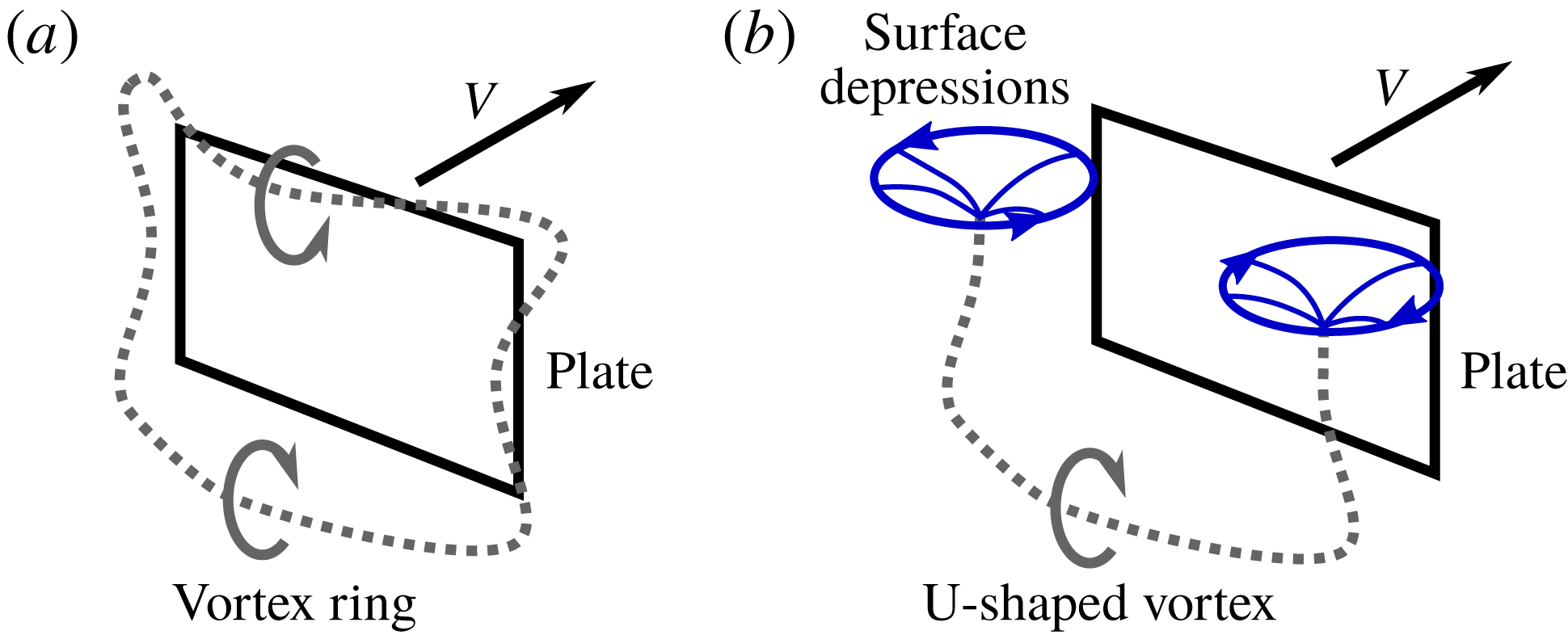
mm, is prevented. Instead, a U-shaped starting vortex is formed, of which the free ends attach to the air–water interface and produce strong depressions in the interface; see figure 8(d). A schematic side-by-side comparison of the vortices in the
$h=100$
mm, is prevented. Instead, a U-shaped starting vortex is formed, of which the free ends attach to the air–water interface and produce strong depressions in the interface; see figure 8(d). A schematic side-by-side comparison of the vortices in the $h=0$
and the
$h=0$
and the $h=100$
mm cases is given in figure 9. During the transition phase the U-shaped vortex detaches and quickly loses strength, visible as the flattening of the bottom of the surface vortices, meaning that they are no longer connected to a strong vortex below; see figure 8(e). Also it appears that the vortex cores are no longer strong enough to capture the hydrogen bubbles in a well-defined core. The shifting away of the surface vortices as well as the break-up of the U-shaped vortex continues until a steady-phase wake similar to that of the deep water case is formed, except that in the case of
$h=100$
mm cases is given in figure 9. During the transition phase the U-shaped vortex detaches and quickly loses strength, visible as the flattening of the bottom of the surface vortices, meaning that they are no longer connected to a strong vortex below; see figure 8(e). Also it appears that the vortex cores are no longer strong enough to capture the hydrogen bubbles in a well-defined core. The shifting away of the surface vortices as well as the break-up of the U-shaped vortex continues until a steady-phase wake similar to that of the deep water case is formed, except that in the case of $h=0$
mm the wake is limited by the free surface, effectively cutting off part of the wake; see figure 8(f).
$h=0$
mm the wake is limited by the free surface, effectively cutting off part of the wake; see figure 8(f).
Vortex formation during the acceleration phase. In the case of $h=100$
mm (a) the plate is fully submerged and a closed vortex ring is formed behind the plate. In the case of
$h=100$
mm (a) the plate is fully submerged and a closed vortex ring is formed behind the plate. In the case of $h=0$
mm (b) the top of the plate coincides with the water surface, and a closed vortex ring cannot be formed. Instead, a U-shaped vortex ring is formed, which attaches to the surface with both ends, creating surface depressions.
$h=0$
mm (b) the top of the plate coincides with the water surface, and a closed vortex ring cannot be formed. Instead, a U-shaped vortex ring is formed, which attaches to the surface with both ends, creating surface depressions.
In the $h=20$
mm case, i.e. the case with maximum drag during the steady phase, the flow behaviour is a mixture of features observed in the flows for the deep water (
$h=20$
mm case, i.e. the case with maximum drag during the steady phase, the flow behaviour is a mixture of features observed in the flows for the deep water ( $h=100$
mm) and surface cases (
$h=100$
mm) and surface cases ( $h=0$
mm). During the acceleration phase both a vortex ring and vortices connected to the air–water interface are formed; see figure 8(g). During the transition phase the surface vortices shed more quickly than in the
$h=0$
mm). During the acceleration phase both a vortex ring and vortices connected to the air–water interface are formed; see figure 8(g). During the transition phase the surface vortices shed more quickly than in the $h=0$
mm case, deforming the vortex ring in streamwise direction; see figure 8(h). After the vortex ring disintegrates a steady wake is formed similar to that of the
$h=0$
mm case, deforming the vortex ring in streamwise direction; see figure 8(h). After the vortex ring disintegrates a steady wake is formed similar to that of the $h=0$
mm case. However, the gap between the top of the plate and the air–water interface causes a flow over the plate creating a large circulation zone closely trailing the plate as indicated in figure 8(i). This creates a low pressure region on the wake side of the plate explaining the maximum drag during the steady phase found for this case.
$h=0$
mm case. However, the gap between the top of the plate and the air–water interface causes a flow over the plate creating a large circulation zone closely trailing the plate as indicated in figure 8(i). This creates a low pressure region on the wake side of the plate explaining the maximum drag during the steady phase found for this case.
3.6 Large flow structures
Figure 5 shows that the maximum drag is reached at the end of the acceleration phase for all three cases. During the acceleration phase the drag is mainly due to acceleration of the plate mass $m_{p}$
and the hydrodynamic mass
$m_{p}$
and the hydrodynamic mass $m_{h}$
. One would expect the plate deepest submerged to entrain most water and therefore to have the largest hydrodynamic mass. However, it is clear that both the
$m_{h}$
. One would expect the plate deepest submerged to entrain most water and therefore to have the largest hydrodynamic mass. However, it is clear that both the $h=0$
mm and the
$h=0$
mm and the $h=20$
mm cases have a higher initial peak. This is caused by the observed strong surface vortices formed in these two cases, resulting in strong low pressure zones close to the plate, and thus creating a larger drag. One more difference is the observed peaks 1 and 2 in the drag force signal for the
$h=20$
mm cases have a higher initial peak. This is caused by the observed strong surface vortices formed in these two cases, resulting in strong low pressure zones close to the plate, and thus creating a larger drag. One more difference is the observed peaks 1 and 2 in the drag force signal for the $h=100$
mm case, which are not observed in the force signals for the
$h=100$
mm case, which are not observed in the force signals for the $h=0$
mm and
$h=0$
mm and $h=20$
mm cases. It is observed that in the case of
$h=20$
mm cases. It is observed that in the case of $h=100$
mm several large vortical structures are formed and shed during the transition phase, instead of just the formation of a starting vortex. The structures are of similar size and shape as the starting vortex, although less defined, and their creation and shedding coincides with peaks 1 and 2.
$h=100$
mm several large vortical structures are formed and shed during the transition phase, instead of just the formation of a starting vortex. The structures are of similar size and shape as the starting vortex, although less defined, and their creation and shedding coincides with peaks 1 and 2.
Coming back to the observed trend break at $h=50$
mm in figure 4, we speculate that at this depth two drag enhancing mechanisms play a role as stated in § 3.3. Firstly, a circulation zone is formed close to the plate, as is discussed in § 3.5. This circulation zone increasingly enhances plate drag from
$h=50$
mm in figure 4, we speculate that at this depth two drag enhancing mechanisms play a role as stated in § 3.3. Firstly, a circulation zone is formed close to the plate, as is discussed in § 3.5. This circulation zone increasingly enhances plate drag from $h=0$
to
$h=0$
to $h=20$
mm where this effect reaches its maximum. We further speculate that as the gap between the top of the plate and the free surface increases, from
$h=20$
mm where this effect reaches its maximum. We further speculate that as the gap between the top of the plate and the free surface increases, from $h=20$
to
$h=20$
to $h=50$
mm, the circulation zone weakens and consequently the plate drag decreases. The second drag enhancing mechanism is the growth of the wake size, i.e. the wake height, with increasing plate depth. Since the separation points on the flat plate are well defined due to the sharp edges of the plate, unlike e.g. the separation points on a cylinder which vary with Reynolds number (Williamson Reference Williamson1996), the drag on the flat plate and the wake size of the flat plate, i.e. the wake height, are positively correlated. At larger plate depths a smaller part of the wake is clipped by the free surface, and consequently, a larger mass of water is entrained in the plate wake thus increasing the plate drag. Figure 4 indicates that the drag during the steady phase for the
$h=50$
mm, the circulation zone weakens and consequently the plate drag decreases. The second drag enhancing mechanism is the growth of the wake size, i.e. the wake height, with increasing plate depth. Since the separation points on the flat plate are well defined due to the sharp edges of the plate, unlike e.g. the separation points on a cylinder which vary with Reynolds number (Williamson Reference Williamson1996), the drag on the flat plate and the wake size of the flat plate, i.e. the wake height, are positively correlated. At larger plate depths a smaller part of the wake is clipped by the free surface, and consequently, a larger mass of water is entrained in the plate wake thus increasing the plate drag. Figure 4 indicates that the drag during the steady phase for the $h=0$
mm case is significantly lower than that for the deep water case (
$h=0$
mm case is significantly lower than that for the deep water case ( $h=100$
mm). The wake size of the surface case (
$h=100$
mm). The wake size of the surface case ( $h=0$
mm), is only approximately 75 % of the size of the deep water case (
$h=0$
mm), is only approximately 75 % of the size of the deep water case ( $h=100$
mm); see figures 8(c) and 8(f). The ratio of drag coefficients
$h=100$
mm); see figures 8(c) and 8(f). The ratio of drag coefficients $C_{D0mm}/C_{D100mm}\approx 0.8$
reflects the ratio of the wake sizes in the vertical direction (
$C_{D0mm}/C_{D100mm}\approx 0.8$
reflects the ratio of the wake sizes in the vertical direction ( ${\approx}0.75$
), which is in accordance with our hypothesis that the drag and wake size are positively correlated. Finally, in figure 4 a local maximum at
${\approx}0.75$
), which is in accordance with our hypothesis that the drag and wake size are positively correlated. Finally, in figure 4 a local maximum at $h=100$
mm can be seen, although less pronounced than the maximum at
$h=100$
mm can be seen, although less pronounced than the maximum at $h=20$
mm. We hypothesise that this local maximum or trend break is caused by weakening interactions between the plate wake and the free surface.
$h=20$
mm. We hypothesise that this local maximum or trend break is caused by weakening interactions between the plate wake and the free surface.
In the next sections (§§ 3.7 and 3.8) the instantaneous force signal during the acceleration and transition phase is discussed. For a further analysis of the large structures on the basis of PIV measurements we refer the reader to §§ 3.9 and 3.10.
3.7 Alternative modelling of the hydrodynamic mass
As observed in the flow visualisations the entrained mass in the wake of the plate during the acceleration phase is not constant, but grows larger over time, and so does the plate drag force. This suggests an increasing hydrodynamic mass $m_{h}$
over time, instead of a constant hydrodynamic mass as suggested by Patton (Reference Patton1965) and Yu (Reference Yu1945). Moreover, due to the acceleration strong vortices are formed close to the plate that increase the drag on the plate even further through their pressure fields. To investigate the variation of the hydrodynamic mass over time, experiments are carried out for different combinations of plate velocity, acceleration and plate depth. Each combination of velocity (
$m_{h}$
over time, instead of a constant hydrodynamic mass as suggested by Patton (Reference Patton1965) and Yu (Reference Yu1945). Moreover, due to the acceleration strong vortices are formed close to the plate that increase the drag on the plate even further through their pressure fields. To investigate the variation of the hydrodynamic mass over time, experiments are carried out for different combinations of plate velocity, acceleration and plate depth. Each combination of velocity ( $V=0.20$
, 0.25, 0.30, 0.35,
$V=0.20$
, 0.25, 0.30, 0.35, $0.40~\text{m}~\text{s}^{-1}$
) and acceleration (
$0.40~\text{m}~\text{s}^{-1}$
) and acceleration ( $a=0.41$
, 0.62, 0.82, 1.02 1.23, 1.44,
$a=0.41$
, 0.62, 0.82, 1.02 1.23, 1.44, $1.64~\text{m}~\text{s}^{-2}$
) is tested for each depth (
$1.64~\text{m}~\text{s}^{-2}$
) is tested for each depth ( $h=0$
, 20, 100 mm) resulting in 105 measurements. Figure 10 shows the effects of variations in acceleration
$h=0$
, 20, 100 mm) resulting in 105 measurements. Figure 10 shows the effects of variations in acceleration $a$
and target velocity
$a$
and target velocity $V$
on the drag force
$V$
on the drag force $F_{x}$
as function of time; note that from here on, all force signals are filtered to improve readability using a second-order Savitzky–Golay filter with a 0.1 s window. During the steady phase the plate drag scales with
$F_{x}$
as function of time; note that from here on, all force signals are filtered to improve readability using a second-order Savitzky–Golay filter with a 0.1 s window. During the steady phase the plate drag scales with $F_{x}\sim V^{2}$
as is expected from (3.2); see figure 10(b). However, during the acceleration phase, the plate drag appears to increase linearly with time
$F_{x}\sim V^{2}$
as is expected from (3.2); see figure 10(b). However, during the acceleration phase, the plate drag appears to increase linearly with time $F_{x}\sim t$
which for constant acceleration is identical to
$F_{x}\sim t$
which for constant acceleration is identical to $F_{x}\sim V$
(figure 10
b), and is not in agreement with (3.2). Also, the increase of the plate drag with respect to time, i.e. the rate of change
$F_{x}\sim V$
(figure 10
b), and is not in agreement with (3.2). Also, the increase of the plate drag with respect to time, i.e. the rate of change $\text{d}F/\text{d}t$
, appears to scale with acceleration
$\text{d}F/\text{d}t$
, appears to scale with acceleration $\text{d}F_{x}/\text{d}t\sim a$
; see figure 10(a).
$\text{d}F_{x}/\text{d}t\sim a$
; see figure 10(a).
Drag force signals $F_{x}(t)$
measured at plate depth
$F_{x}(t)$
measured at plate depth $h=100$
mm. (a)
$h=100$
mm. (a) $F_{x}(t)$
for various accelerations towards a fixed plate velocity
$F_{x}(t)$
for various accelerations towards a fixed plate velocity $V=0.30~\text{m}~\text{s}^{-1}$
. (b)
$V=0.30~\text{m}~\text{s}^{-1}$
. (b) $F_{x}(t)$
for a fixed acceleration of
$F_{x}(t)$
for a fixed acceleration of $a=0.82~\text{m}~\text{s}^{-2}$
towards various plate velocities
$a=0.82~\text{m}~\text{s}^{-2}$
towards various plate velocities $V$
.
$V$
.
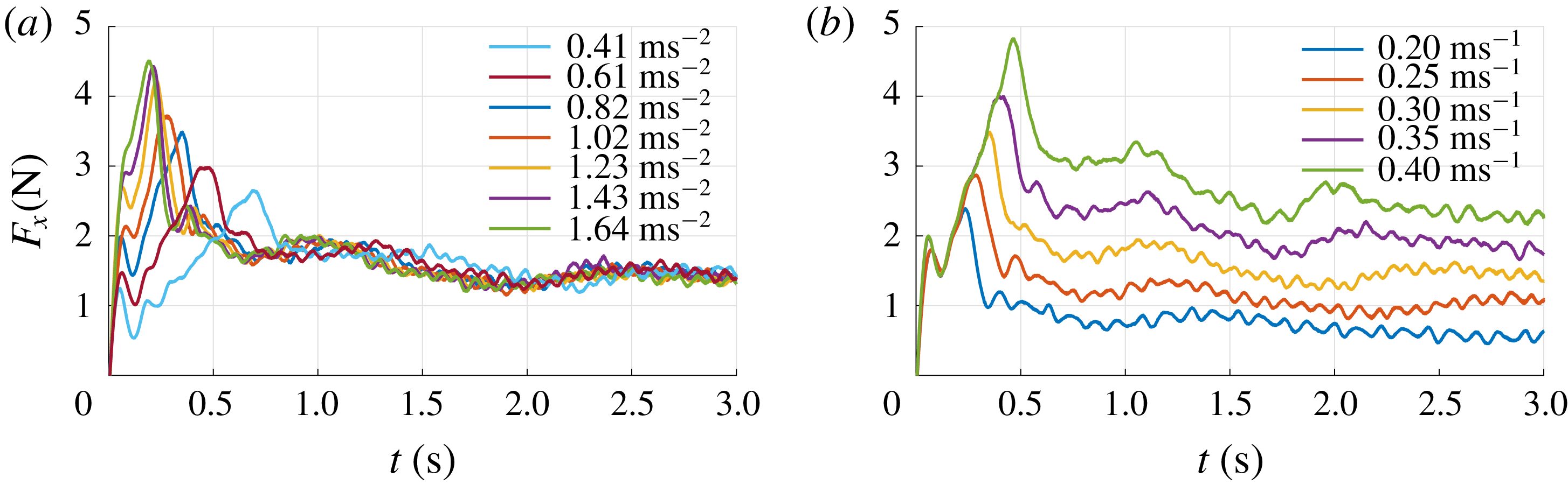
To investigate the increase in force with time during the acceleration phase, the common force decomposition (3.2), is rewritten such that a residual force due to the acceleration of the hydrodynamic mass $m_{h}$
is defined:
$m_{h}$
is defined:
 $$\begin{eqnarray}F_{mh}=F_{x}-\underbrace{m_{p}a(t)}_{F_{mp}}-\underbrace{{\textstyle \frac{1}{2}}\unicode[STIX]{x1D70C}V(t)^{2}C_{D}A}_{F_{CD}}.\end{eqnarray}$$
This modelling choice effectively isolates the increase in drag due to unsteady effects. For small movements starting from rest, the residual force $F_{mh}$
matches the product of the acceleration
$F_{mh}$
matches the product of the acceleration $a$
and the hydrodynamic mass
$a$
and the hydrodynamic mass $m_{h}$
from (3.4) as proposed by Yu (Reference Yu1945); see the markers in figure 11(a). Note that a small offset in time, equal to
$m_{h}$
from (3.4) as proposed by Yu (Reference Yu1945); see the markers in figure 11(a). Note that a small offset in time, equal to $t_{sr}=0.07$
s, takes into account the step response. Since the behaviour of the force signal during the acceleration phase is independent of the target velocity
$t_{sr}=0.07$
s, takes into account the step response. Since the behaviour of the force signal during the acceleration phase is independent of the target velocity $V$
(figure 10
b), we use the measurements with the highest target velocity of
$V$
(figure 10
b), we use the measurements with the highest target velocity of $V=0.40~\text{m}~\text{s}^{-1}$
to fit a model, as these data contain the longest acceleration time. Figure 11(a) shows linear fits through the theoretical added mass as proposed by Yu (Reference Yu1945), with a fit for each signal defined as:
$V=0.40~\text{m}~\text{s}^{-1}$
to fit a model, as these data contain the longest acceleration time. Figure 11(a) shows linear fits through the theoretical added mass as proposed by Yu (Reference Yu1945), with a fit for each signal defined as:
 $$\begin{eqnarray}F_{mh}=\frac{\text{d}F_{mh}}{\text{d}t}(t-t_{sr})+m_{h(Yu)}a,\end{eqnarray}$$
where the only free fitting parameter is the rate of change of the residual force $\text{d}F_{mh}/\text{d}t$
. In figure 11(b) all found rates of change of force
$\text{d}F_{mh}/\text{d}t$
. In figure 11(b) all found rates of change of force $\text{d}F/\text{d}t$
are plotted as a function of acceleration
$\text{d}F/\text{d}t$
are plotted as a function of acceleration $a$
. The markers show the values of
$a$
. The markers show the values of $\text{d}F/\text{d}t$
for different accelerations for the three selected depths, while the lines indicate the clear linear behaviour of
$\text{d}F/\text{d}t$
for different accelerations for the three selected depths, while the lines indicate the clear linear behaviour of $\text{d}F/\text{d}t$
with respect to acceleration. To give a physical interpretation to this, it is assumed that the residual force
$\text{d}F/\text{d}t$
with respect to acceleration. To give a physical interpretation to this, it is assumed that the residual force $F_{mh}$
during the acceleration phase is due to the acceleration of the hydrodynamic mass in the wake of the plate. Note that this assumption does not necessarily capture the intricate phenomena of the formation of the ring vortex or the subsequent deformation of the free surface, which possibly increase the plate drag via other mechanisms than entrainment. However, this assumption does enable us to model the enhanced plate drag in a simple and convenient manner. We define the residual force as:
$F_{mh}$
during the acceleration phase is due to the acceleration of the hydrodynamic mass in the wake of the plate. Note that this assumption does not necessarily capture the intricate phenomena of the formation of the ring vortex or the subsequent deformation of the free surface, which possibly increase the plate drag via other mechanisms than entrainment. However, this assumption does enable us to model the enhanced plate drag in a simple and convenient manner. We define the residual force as:
 $$\begin{eqnarray}F_{mh}=m_{h}a,\end{eqnarray}$$
where the hydrodynamic mass $m_{h}$
is time dependent since the acceleration
$m_{h}$
is time dependent since the acceleration $a$
is constant for each measurement, while
$a$
is constant for each measurement, while $F_{mh}$
is increasing in time. This leads to the definition of the entrainment rate of mass in the wake of the plate:
$F_{mh}$
is increasing in time. This leads to the definition of the entrainment rate of mass in the wake of the plate:
 $$\begin{eqnarray}\frac{\text{d}m_{h}}{\text{d}t}=\frac{1}{a}\frac{\text{d}F_{mh}}{\text{d}t},\end{eqnarray}$$
shown as a function of the acceleration $a$
in figure 11(c). When the plate is at the free surface (
$a$
in figure 11(c). When the plate is at the free surface ( $h=0$
mm) the entrainment rate
$h=0$
mm) the entrainment rate $\text{d}m_{h}/\text{d}t$
is strongly enhanced when compared to the deeper immersed plates; at lower accelerations this almost doubles. Also, we show that for all three selected plate depths the entrainment rate is gradually increasing with acceleration up to
$\text{d}m_{h}/\text{d}t$
is strongly enhanced when compared to the deeper immersed plates; at lower accelerations this almost doubles. Also, we show that for all three selected plate depths the entrainment rate is gradually increasing with acceleration up to $a\approx 1~\text{m}~\text{s}^{-2}$
, while for higher accelerations the entrainment rate has a constant value. At a higher entrainment rate the wake grows more rapidly over time thus faster increasing the plate drag force. The maximum force experienced by the plate during uniform acceleration is the sum of the steady phase drag force
$a\approx 1~\text{m}~\text{s}^{-2}$
, while for higher accelerations the entrainment rate has a constant value. At a higher entrainment rate the wake grows more rapidly over time thus faster increasing the plate drag force. The maximum force experienced by the plate during uniform acceleration is the sum of the steady phase drag force $F_{CD}$
and the residual force
$F_{CD}$
and the residual force $F_{mh}$
, which are both dependent on immersion depth
$F_{mh}$
, which are both dependent on immersion depth $h$
as shown in figures 4 and 11(c), respectively. The maximum force achieved at some depth
$h$
as shown in figures 4 and 11(c), respectively. The maximum force achieved at some depth $h$
is then dependent on the set target velocity
$h$
is then dependent on the set target velocity $V$
and acceleration
$V$
and acceleration $a$
. Apparently a trade-off exists between steady-phase drag and entrainment, e.g. the case
$a$
. Apparently a trade-off exists between steady-phase drag and entrainment, e.g. the case $h=0$
mm has the lowest steady-phase drag coefficient but has the highest entrainment rate.
$h=0$
mm has the lowest steady-phase drag coefficient but has the highest entrainment rate.
(a) The solid line represents the residual force $F_{mh}$
as function of time (
$F_{mh}$
as function of time ( $t$
) for different accelerations towards a fixed plate velocity
$t$
) for different accelerations towards a fixed plate velocity $V=0.40~\text{m}~\text{s}^{-1}$
at plate depth
$V=0.40~\text{m}~\text{s}^{-1}$
at plate depth $h=0$
mm. The markers represent the force due to hydrodynamic mass as proposed by Yu (Reference Yu1945). The dashed line represents a linear fit through the force signal
$h=0$
mm. The markers represent the force due to hydrodynamic mass as proposed by Yu (Reference Yu1945). The dashed line represents a linear fit through the force signal $F_{mh}(t)$
during the acceleration phase. The vertical dotted line marks the time offset
$F_{mh}(t)$
during the acceleration phase. The vertical dotted line marks the time offset $t_{sr}$
to account for the step response. (b) The rate of change of force
$t_{sr}$
to account for the step response. (b) The rate of change of force $\text{d}F/\text{d}t$
as function of the accelerations
$\text{d}F/\text{d}t$
as function of the accelerations $a$
for the selected plate depths. (c) The entrainment rate
$a$
for the selected plate depths. (c) The entrainment rate $\text{d}m_{h}/\text{d}t$
as function of acceleration
$\text{d}m_{h}/\text{d}t$
as function of acceleration $a$
for the three selected plate depths.
$a$
for the three selected plate depths.
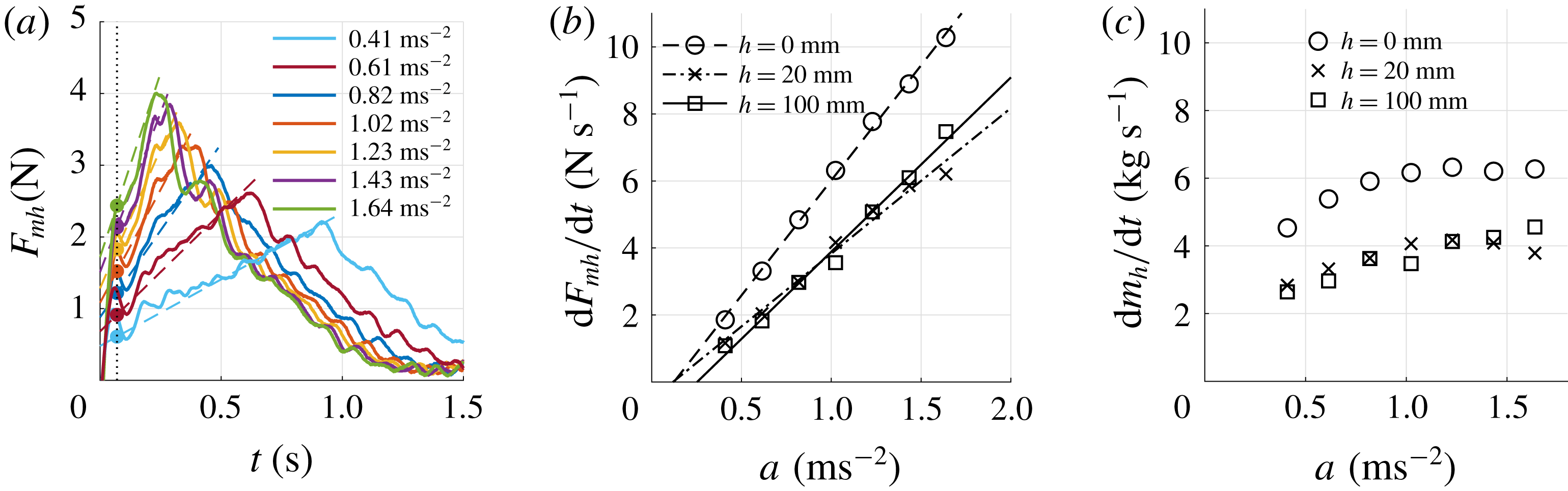
3.8 Force during the transition phase
Figure 11(a) shows that the residual force $F_{mh}$
does not vanish immediately after the plate reaches its target velocity (i.e. when
$F_{mh}$
does not vanish immediately after the plate reaches its target velocity (i.e. when $a$
reaches
$a$
reaches $0~\text{m}~\text{s}^{-2}$
), although this would be expected from the general definition; see (3.7). Instead, the force
$0~\text{m}~\text{s}^{-2}$
), although this would be expected from the general definition; see (3.7). Instead, the force $F_{mh}$
appears to drop sharply to a non-zero value and then gradually decays to zero, after which the total force
$F_{mh}$
appears to drop sharply to a non-zero value and then gradually decays to zero, after which the total force $F_{x}$
equals the steady-phase drag force
$F_{x}$
equals the steady-phase drag force $F_{CD}$
. The force which vanishes immediately upon
$F_{CD}$
. The force which vanishes immediately upon $a$
reaching 0 we call a ‘force due to added mass’, since it relates to the acceleration of the plate. The gradually decreasing force we call a ‘history force’, which is due to the developing wake caused by the past acceleration of the plate, which exists long after the plate reaches its target velocity. This is analogues to the virtual mass force for a spherical particle:
$a$
reaching 0 we call a ‘force due to added mass’, since it relates to the acceleration of the plate. The gradually decreasing force we call a ‘history force’, which is due to the developing wake caused by the past acceleration of the plate, which exists long after the plate reaches its target velocity. This is analogues to the virtual mass force for a spherical particle: $F=(\unicode[STIX]{x1D70C}_{c}V_{p}/2)(\text{D}\boldsymbol{u}/\text{D}t-\text{d}\boldsymbol{v}/\text{d}t)$
(Crowe et al.
Reference Crowe, Schwarzkopf, Sommerfeld and Tsuji2011), where
$F=(\unicode[STIX]{x1D70C}_{c}V_{p}/2)(\text{D}\boldsymbol{u}/\text{D}t-\text{d}\boldsymbol{v}/\text{d}t)$
(Crowe et al.
Reference Crowe, Schwarzkopf, Sommerfeld and Tsuji2011), where $\unicode[STIX]{x1D70C}_{c}V_{p}/2$
is the displaced fluid mass,
$\unicode[STIX]{x1D70C}_{c}V_{p}/2$
is the displaced fluid mass, $\text{d}\boldsymbol{v}/\text{d}t$
the particle acceleration (added mass term) and
$\text{d}\boldsymbol{v}/\text{d}t$
the particle acceleration (added mass term) and $\text{D}\boldsymbol{u}/\text{D}t$
the material derivative of the fluid (history term).
$\text{D}\boldsymbol{u}/\text{D}t$
the material derivative of the fluid (history term).
We assume that the plate reaches the constant target velocity at time $t_{c}$
and location
$t_{c}$
and location $x_{c}$
. As discussed in § 3.5 the acceleration and transition phase are dominated by the formation and shedding of vortices. As discussed in § 1.3, a suitable dimensionless time to describe these flow phenomena is
$x_{c}$
. As discussed in § 3.5 the acceleration and transition phase are dominated by the formation and shedding of vortices. As discussed in § 1.3, a suitable dimensionless time to describe these flow phenomena is $t^{\ast }$
, i.e. the ‘formation time’, defined as
$t^{\ast }$
, i.e. the ‘formation time’, defined as
 $$\begin{eqnarray}t^{\ast }=\frac{1}{l_{b}}\int _{0}^{t}V(\unicode[STIX]{x1D70F})\,\text{d}\unicode[STIX]{x1D70F},\end{eqnarray}$$
where $V(t)$
is the instantaneous velocity at time
$V(t)$
is the instantaneous velocity at time $t$
, and
$t$
, and $l_{b}$
a characteristic length, which here is chosen to be the plate height. The non-dimensional time
$l_{b}$
a characteristic length, which here is chosen to be the plate height. The non-dimensional time $t^{\ast }$
is then effectively the number of plate heights travelled, which is identical to the non-dimensional time used in the simulations by Koumoutsakos & Shiels (Reference Koumoutsakos and Shiels1996).
$t^{\ast }$
is then effectively the number of plate heights travelled, which is identical to the non-dimensional time used in the simulations by Koumoutsakos & Shiels (Reference Koumoutsakos and Shiels1996).
The residual force in dimensional form $F_{mh}$
(a,c) and non-dimensional form
$F_{mh}$
(a,c) and non-dimensional form $F^{\ast }$
(b,d) as a function of the post-acceleration time
$F^{\ast }$
(b,d) as a function of the post-acceleration time $t-t_{c}$
or formation time
$t-t_{c}$
or formation time $t^{\ast }-t_{c}^{\ast }$
for different accelerations towards a fixed plate velocity
$t^{\ast }-t_{c}^{\ast }$
for different accelerations towards a fixed plate velocity $V=0.30~\text{m}~\text{s}^{-1}$
(a,b) or towards different velocities at a fixed acceleration
$V=0.30~\text{m}~\text{s}^{-1}$
(a,b) or towards different velocities at a fixed acceleration $a=0.82~\text{m}~\text{s}^{-2}$
(c,d) for plate depth
$a=0.82~\text{m}~\text{s}^{-2}$
(c,d) for plate depth $h=100$
mm. In (a,b) the dashed line indicates the dimensionless step response time
$h=100$
mm. In (a,b) the dashed line indicates the dimensionless step response time $t_{sr}^{\ast }$
. In (d) the dotted lines indicate the locations of peak 1 and peak 2 which for different velocities coalesce in non-dimensional time. (a) Residual force as function of post-acceleration formation time for
$t_{sr}^{\ast }$
. In (d) the dotted lines indicate the locations of peak 1 and peak 2 which for different velocities coalesce in non-dimensional time. (a) Residual force as function of post-acceleration formation time for $h=100$
mm, velocity
$h=100$
mm, velocity $V=0.30~\text{m}~\text{s}^{-1}$
and varying accelerations. (b) Normalised residual force as function of post-acceleration formation time for
$V=0.30~\text{m}~\text{s}^{-1}$
and varying accelerations. (b) Normalised residual force as function of post-acceleration formation time for $h=100$
mm, velocity
$h=100$
mm, velocity $V=0.30~\text{m}~\text{s}^{-1}$
and varying accelerations. (c) Residual force as function of post-acceleration time for
$V=0.30~\text{m}~\text{s}^{-1}$
and varying accelerations. (c) Residual force as function of post-acceleration time for $h=100$
mm, acceleration
$h=100$
mm, acceleration $a=0.82~\text{m}~\text{s}^{-2}$
and varying velocities. (d) Normalised residual force as function of post-acceleration formation time for
$a=0.82~\text{m}~\text{s}^{-2}$
and varying velocities. (d) Normalised residual force as function of post-acceleration formation time for $h=100$
mm, acceleration
$h=100$
mm, acceleration $a=0.82~\text{m}~\text{s}^{-2}$
and varying velocities.
$a=0.82~\text{m}~\text{s}^{-2}$
and varying velocities.
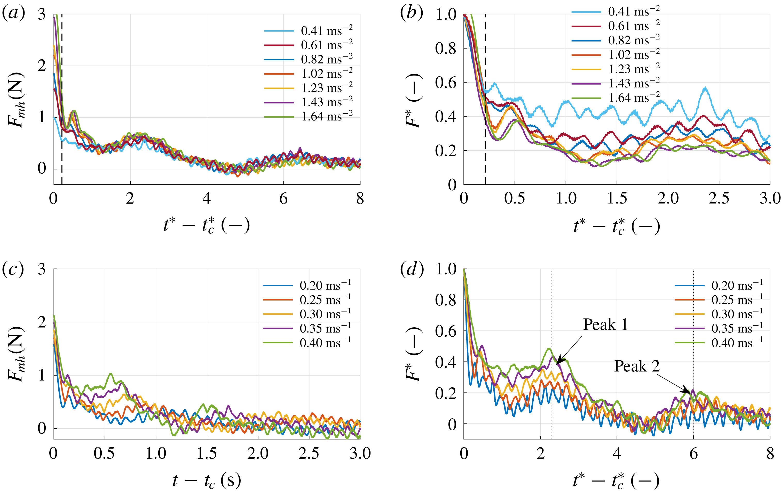
Figure 12 shows the drag force signal as a function of the post-acceleration formation time $t^{\ast }-t_{c}^{\ast }$
during the early transition phase for a plate depth
$t^{\ast }-t_{c}^{\ast }$
during the early transition phase for a plate depth $h=100$
mm and a velocity
$h=100$
mm and a velocity $V=0.30~\text{m}~\text{s}^{-1}$
. Note that
$V=0.30~\text{m}~\text{s}^{-1}$
. Note that $t^{\ast }$
at constant velocity linearly increases with dimensional time
$t^{\ast }$
at constant velocity linearly increases with dimensional time $t$
. As shown in figure 12(a) the force signals
$t$
. As shown in figure 12(a) the force signals $F_{mh}$
quickly decrease when the acceleration ends and converge after
$F_{mh}$
quickly decrease when the acceleration ends and converge after $t^{\ast }-t_{c}^{\ast }\approx 1$
, i.e. when the plate has travelled at constant velocity
$t^{\ast }-t_{c}^{\ast }\approx 1$
, i.e. when the plate has travelled at constant velocity $V$
over a distance of a single plate height
$V$
over a distance of a single plate height $l_{b}$
. This implies that the varying accelerations at which the plate accelerated to its target velocity do not cause lasting effects in the flow beyond the travelled distance of a single plate height
$l_{b}$
. This implies that the varying accelerations at which the plate accelerated to its target velocity do not cause lasting effects in the flow beyond the travelled distance of a single plate height $l_{b}$
. Next, we introduce the normalised force
$l_{b}$
. Next, we introduce the normalised force $F^{\ast }$
defined as
$F^{\ast }$
defined as
 $$\begin{eqnarray}F^{\ast }=\frac{F_{mh}}{F_{mh}(t_{c})},\end{eqnarray}$$
where the residual force $F_{mh}$
is normalised by its maximum value at time
$F_{mh}$
is normalised by its maximum value at time $t_{c}$
. In figure 12(b) it can be seen that the normalised force
$t_{c}$
. In figure 12(b) it can be seen that the normalised force $F^{\ast }$
immediately after the acceleration ends, thus within the step response time of the force signal due to the abrupt change in force on the plate (indicated by the dashed line), the force has decreased by 50–70 %. The initial decrease appears to scale with acceleration, i.e. force signals based on a higher acceleration have a larger initial decrease, while for lower acceleration the initial decrease is smaller. This implies that the added mass force is dominant for higher accelerations, while for lower accelerations
$F^{\ast }$
immediately after the acceleration ends, thus within the step response time of the force signal due to the abrupt change in force on the plate (indicated by the dashed line), the force has decreased by 50–70 %. The initial decrease appears to scale with acceleration, i.e. force signals based on a higher acceleration have a larger initial decrease, while for lower acceleration the initial decrease is smaller. This implies that the added mass force is dominant for higher accelerations, while for lower accelerations $F_{mh}$
is more like a history force.
$F_{mh}$
is more like a history force.
The force $F_{mh}$
as a function of
$F_{mh}$
as a function of $t-t_{c}$
does not converge for different velocities when
$t-t_{c}$
does not converge for different velocities when $a$
remains constant (see figure 12
c). The normalised force
$a$
remains constant (see figure 12
c). The normalised force $F^{\ast }$
as a function of
$F^{\ast }$
as a function of $t^{\ast }-t_{c}^{\ast }$
does not converge for different velocities either, but the low-frequency peaks, indicated as peak 1 and peak 2, now nicely align in dimensionless time (see figure 12
d). Those peaks are associated with the formation and shedding of large vortical structures in the wake, see § 3.6. It appears that the formation time
$t^{\ast }-t_{c}^{\ast }$
does not converge for different velocities either, but the low-frequency peaks, indicated as peak 1 and peak 2, now nicely align in dimensionless time (see figure 12
d). Those peaks are associated with the formation and shedding of large vortical structures in the wake, see § 3.6. It appears that the formation time $t^{\ast }$
, as proposed by Gharib et al. (Reference Gharib, Rambod and Shariff1998) and applied to a vortex ring generated by a jet, also is a universal time scale for the development of the vortical structures in the wake of the plate. Also, the lower velocities show a larger initial decrease than the higher velocities, indicating that for lower velocities the residual force
$t^{\ast }$
, as proposed by Gharib et al. (Reference Gharib, Rambod and Shariff1998) and applied to a vortex ring generated by a jet, also is a universal time scale for the development of the vortical structures in the wake of the plate. Also, the lower velocities show a larger initial decrease than the higher velocities, indicating that for lower velocities the residual force $F_{mh}$
acts more like a force due to added mass than like a history force.
$F_{mh}$
acts more like a force due to added mass than like a history force.
Figure 13(a) shows that, also for the case of $h=0$
mm for different accelerations towards a fixed plate velocity of
$h=0$
mm for different accelerations towards a fixed plate velocity of $V=0.30~\text{m}~\text{s}^{-1}$
, the force signals converge after the plate has travelled at constant velocity over a distance of a few plate heights, i.e. the plate drag force is no longer affected by the initial acceleration by which the plate reached its target velocity. However, when considering the normalised force
$V=0.30~\text{m}~\text{s}^{-1}$
, the force signals converge after the plate has travelled at constant velocity over a distance of a few plate heights, i.e. the plate drag force is no longer affected by the initial acceleration by which the plate reached its target velocity. However, when considering the normalised force $F^{\ast }$
for the case
$F^{\ast }$
for the case $h=0$
mm, shown in figure 13(b), it is obvious that the initial decrease, i.e. the decrease within the step response time
$h=0$
mm, shown in figure 13(b), it is obvious that the initial decrease, i.e. the decrease within the step response time $t_{sr}^{\ast }$
, is much smaller than for the case of
$t_{sr}^{\ast }$
, is much smaller than for the case of $h=100$
mm (see figure 12
b); 20 %–40 % for
$h=100$
mm (see figure 12
b); 20 %–40 % for $h=0$
mm, compared to 50 %–70 % for
$h=0$
mm, compared to 50 %–70 % for $h=100$
mm. This indicates that the effect of added mass is far less pronounced for the surface case (
$h=100$
mm. This indicates that the effect of added mass is far less pronounced for the surface case ( $h=0$
mm) than it is for the deeper immersed plate (
$h=0$
mm) than it is for the deeper immersed plate ( $h=100$
mm) and that the residual force
$h=100$
mm) and that the residual force $F_{mh}$
for
$F_{mh}$
for $h=0$
mm acts more like a history force than a force due to added mass. Despite the difference in the initial decrease of the residual force and the absence of peak 1 and peak 2 in the force signal for the case of
$h=0$
mm acts more like a history force than a force due to added mass. Despite the difference in the initial decrease of the residual force and the absence of peak 1 and peak 2 in the force signal for the case of $h=0$
mm, the force signal is similar to that of the
$h=0$
mm, the force signal is similar to that of the $h=100$
mm case with respect to changing acceleration: the relative initial decrease is proportional to acceleration.
$h=100$
mm case with respect to changing acceleration: the relative initial decrease is proportional to acceleration.
The residual force in dimensional form $F_{mh}$
(a,c) or non-dimensional form
$F_{mh}$
(a,c) or non-dimensional form $F^{\ast }$
(b,d) as a function of the post-acceleration time
$F^{\ast }$
(b,d) as a function of the post-acceleration time $t-t_{c}$
or formation time
$t-t_{c}$
or formation time $t^{\ast }-t_{c}^{\ast }$
for different accelerations towards a fixed plate velocity
$t^{\ast }-t_{c}^{\ast }$
for different accelerations towards a fixed plate velocity $V=0.30~\text{m}~\text{s}^{-1}$
(a,b) or towards different velocities at a fixed acceleration
$V=0.30~\text{m}~\text{s}^{-1}$
(a,b) or towards different velocities at a fixed acceleration $a=0.82~\text{m}~\text{s}^{-2}$
(c,d) for plate depth
$a=0.82~\text{m}~\text{s}^{-2}$
(c,d) for plate depth $h=0$
mm. In (a,b) the dashed line indicates the dimensionless step response time
$h=0$
mm. In (a,b) the dashed line indicates the dimensionless step response time $t_{sr}^{\ast }$
. (a) Residual force as function of post-acceleration formation time for
$t_{sr}^{\ast }$
. (a) Residual force as function of post-acceleration formation time for $h=0$
mm, velocity
$h=0$
mm, velocity $V=0.30~\text{m}~\text{s}^{-1}$
and varying accelerations. (b) Normalised residual force as function of post-acceleration formation time for
$V=0.30~\text{m}~\text{s}^{-1}$
and varying accelerations. (b) Normalised residual force as function of post-acceleration formation time for $h=0$
mm, velocity
$h=0$
mm, velocity $V=0.30~\text{m}~\text{s}^{-1}$
and varying accelerations. (c) Residual force as function of post-acceleration time for
$V=0.30~\text{m}~\text{s}^{-1}$
and varying accelerations. (c) Residual force as function of post-acceleration time for $h=0$
mm, acceleration
$h=0$
mm, acceleration $a=0.82~\text{m}~\text{s}^{-2}$
and varying velocities. (d) Normalised residual force as function of post-acceleration formation time for
$a=0.82~\text{m}~\text{s}^{-2}$
and varying velocities. (d) Normalised residual force as function of post-acceleration formation time for $h=0$
mm, acceleration
$h=0$
mm, acceleration $a=0.82~\text{m}~\text{s}^{-2}$
and varying velocities.
$a=0.82~\text{m}~\text{s}^{-2}$
and varying velocities.
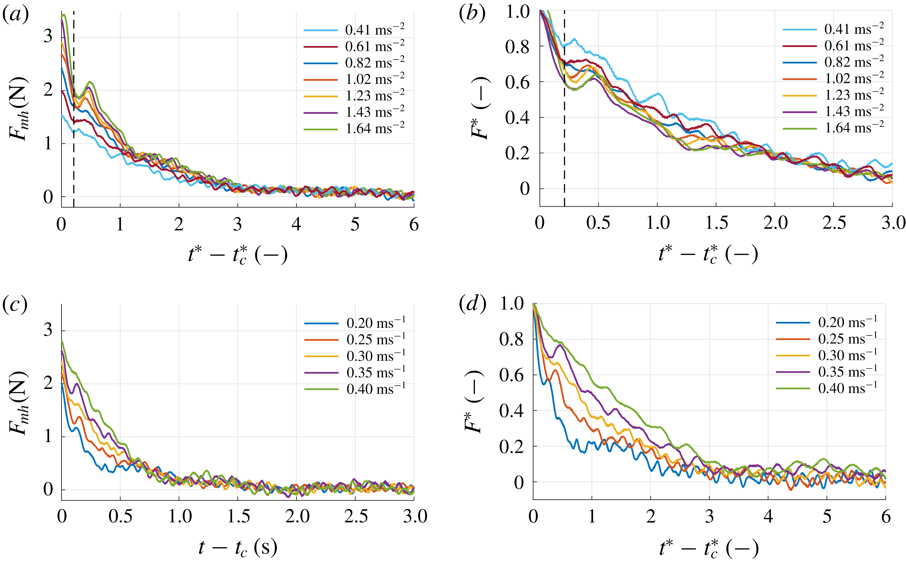
Figure 13 shows the change in force signals during the transition phase for different velocities and a fixed acceleration of $a=0.82~\text{m}~\text{s}^{-2}$
for the case
$a=0.82~\text{m}~\text{s}^{-2}$
for the case $h=0$
mm. Comparison of figures 13(b) and 12(b) shows that the initial decrease for all velocities is again smaller for the case of
$h=0$
mm. Comparison of figures 13(b) and 12(b) shows that the initial decrease for all velocities is again smaller for the case of $h=0$
mm than for the deeper immersed plate
$h=0$
mm than for the deeper immersed plate $h=100$
mm. However, in each case the initial decrease is largest for the smallest velocity and becomes smaller with increasing velocity. Contrary to the deeper immersed plate
$h=100$
mm. However, in each case the initial decrease is largest for the smallest velocity and becomes smaller with increasing velocity. Contrary to the deeper immersed plate $h=100$
mm, the force signal of the
$h=100$
mm, the force signal of the $h=0$
mm case shows no peaks during its decrease in magnitude from acceleration phase to steady phase. Not unexpectedly due to the absence of characteristic features during the transition phase, introducing the formation time
$h=0$
mm case shows no peaks during its decrease in magnitude from acceleration phase to steady phase. Not unexpectedly due to the absence of characteristic features during the transition phase, introducing the formation time $t^{\ast }$
does not seem to better align the force signals in time during the transition phase.
$t^{\ast }$
does not seem to better align the force signals in time during the transition phase.
When considering the force–time signal of the entire run at a depth of $h=0$
mm for different accelerations towards a target velocity of
$h=0$
mm for different accelerations towards a target velocity of $V=0.30~\text{m}~\text{s}^{-1}$
, shown in figure 14(a), we see that the signals do not converge until
$V=0.30~\text{m}~\text{s}^{-1}$
, shown in figure 14(a), we see that the signals do not converge until $t=1.5$
s. However, when introducing the formation time
$t=1.5$
s. However, when introducing the formation time $t^{\ast }$
we clearly see that all force signals collapse on a single curve during the transition phase; see figure 14(b). Different target velocities each appear to have their own unique curve to which force signals from different accelerations collapse, as shown in figure 15. The curve to which all signals collapse are of the form
$t^{\ast }$
we clearly see that all force signals collapse on a single curve during the transition phase; see figure 14(b). Different target velocities each appear to have their own unique curve to which force signals from different accelerations collapse, as shown in figure 15. The curve to which all signals collapse are of the form $c_{1}/(x-c_{2})^{2}$
with
$c_{1}/(x-c_{2})^{2}$
with $c_{1}$
and
$c_{1}$
and $c_{2}$
increasing with increasing target velocity
$c_{2}$
increasing with increasing target velocity $V$
. The fitting coefficients are shown in the legend of figure 15. The shapes of these curves appear to be determined in full by the target velocity. The formation number from which a force signal starts following this curve depends on the acceleration only. We consider a scaling argument to interpret the behaviour of the force signal by
$V$
. The fitting coefficients are shown in the legend of figure 15. The shapes of these curves appear to be determined in full by the target velocity. The formation number from which a force signal starts following this curve depends on the acceleration only. We consider a scaling argument to interpret the behaviour of the force signal by $1\sim 1/x^{2}$
. From the definition of the formation time
$1\sim 1/x^{2}$
. From the definition of the formation time $t^{\ast }$
, equation (3.9), it is obvious that
$t^{\ast }$
, equation (3.9), it is obvious that $t^{\ast }$
is identical to the plate travel distance
$t^{\ast }$
is identical to the plate travel distance $x(t)$
expressed in the number of plate heights
$x(t)$
expressed in the number of plate heights $l_{b}$
. The flow visualisation showed that the acceleration phase is dominated by the generation of a large starting vortex which is shed upon reaching the target velocity; see § 3.5. Upon shedding this starting vortex quickly becomes irrotational since it is no longer subject to an external force. Let
$l_{b}$
. The flow visualisation showed that the acceleration phase is dominated by the generation of a large starting vortex which is shed upon reaching the target velocity; see § 3.5. Upon shedding this starting vortex quickly becomes irrotational since it is no longer subject to an external force. Let $U$
be the flow velocity of such an irrotational vortex that scales with the inverse of the distance to this vortex
$U$
be the flow velocity of such an irrotational vortex that scales with the inverse of the distance to this vortex $U\sim 1/x$
. Since dynamic pressure
$U\sim 1/x$
. Since dynamic pressure $q$
scales with velocity squared
$q$
scales with velocity squared $q\sim U^{2}$
we can state that the dynamic pressure at the wake side of the plate due to the shed vortex scales with
$q\sim U^{2}$
we can state that the dynamic pressure at the wake side of the plate due to the shed vortex scales with $q\sim 1/x^{2}$
. For the sake of simplicity we assume that we can use Bernoulli’s principle for incompressible irrotational flow such that the total pressure
$q\sim 1/x^{2}$
. For the sake of simplicity we assume that we can use Bernoulli’s principle for incompressible irrotational flow such that the total pressure $P$
is constant throughout the flow, i.e.
$P$
is constant throughout the flow, i.e. $P=p+q$
. We state that the static pressure
$P=p+q$
. We state that the static pressure $p$
increases over plate travel distance as
$p$
increases over plate travel distance as $q$
decreases by
$q$
decreases by ${\sim}1/x^{2}$
. Since the plate drag is the difference in static pressure over the plate, an increase in static pressure at the wake side of the plate implies a decrease in drag force on the plate. This scaling argument matches the observed behaviour
${\sim}1/x^{2}$
. Since the plate drag is the difference in static pressure over the plate, an increase in static pressure at the wake side of the plate implies a decrease in drag force on the plate. This scaling argument matches the observed behaviour $F_{mh}\sim 1/x^{2}$
.
$F_{mh}\sim 1/x^{2}$
.
Force versus time $t$
and the formation time
$t$
and the formation time $t^{\ast }$
for varying accelerations towards
$t^{\ast }$
for varying accelerations towards $V=0.30~\text{m}~\text{s}^{-1}$
at depth
$V=0.30~\text{m}~\text{s}^{-1}$
at depth $h=0$
mm. (a) Dimensional time
$h=0$
mm. (a) Dimensional time $t$
. (b) Formation time
$t$
. (b) Formation time $t^{\ast }$
.
$t^{\ast }$
.
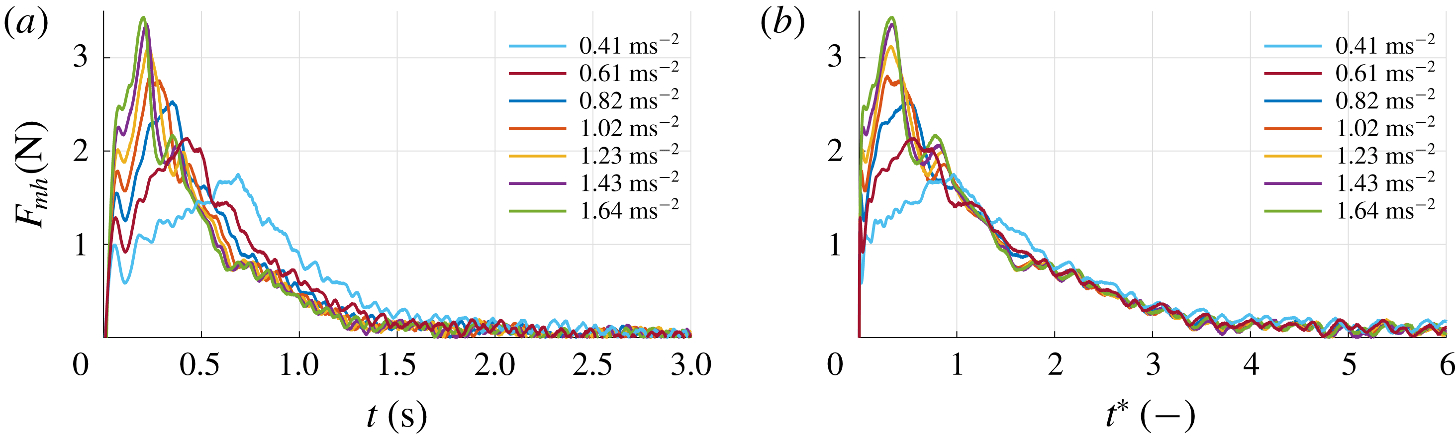
Force signal $F_{mh}$
versus formation time
$F_{mh}$
versus formation time $t^{\ast }$
during the transition phase for different accelerations towards different velocities (solid lines). Fits of the form
$t^{\ast }$
during the transition phase for different accelerations towards different velocities (solid lines). Fits of the form $c_{1}/(t^{\ast }-c_{2})^{2}$
through each set of force signals corresponding to a single velocity (dashed lines).
$c_{1}/(t^{\ast }-c_{2})^{2}$
through each set of force signals corresponding to a single velocity (dashed lines).

3.9 Vorticity
The flow field was analysed using PIV to provide a quantitative insight and to reveal the more intricate structures in the flow that were not captured by the visualisations. Although the flow is highly three-dimensional, as is evident from figure 8, two-component planar PIV still reveals interesting differences, and similarities, between the three selected cases $h=0$
, 20 and 100 mm.
$h=0$
, 20 and 100 mm.
The PIV measurements are done in the horizontal mid-plane of the plate for all three selected plate depths $h=0$
, 20 and 100 mm, at an acceleration of
$h=0$
, 20 and 100 mm, at an acceleration of $a=0.82~\text{m}~\text{s}^{-1}$
, and a target plate velocity
$a=0.82~\text{m}~\text{s}^{-1}$
, and a target plate velocity $V=0.30~\text{m}~\text{s}^{-1}$
. The chosen parameters correspond with the three force measurement results shown in figure 5 and discussed in § 3.3. The PIV results are represented through the vorticity
$V=0.30~\text{m}~\text{s}^{-1}$
. The chosen parameters correspond with the three force measurement results shown in figure 5 and discussed in § 3.3. The PIV results are represented through the vorticity $\unicode[STIX]{x1D714}_{z}$
based on the local flow circulation by an 8-point estimation (Luff et al.
Reference Luff, Drouillard, Rompage, Linne and Hertzberg1999). A discrete representation is used (Adrian & Westerweel Reference Adrian and Westerweel2011) since it allows for different spacing between vectors in the
$\unicode[STIX]{x1D714}_{z}$
based on the local flow circulation by an 8-point estimation (Luff et al.
Reference Luff, Drouillard, Rompage, Linne and Hertzberg1999). A discrete representation is used (Adrian & Westerweel Reference Adrian and Westerweel2011) since it allows for different spacing between vectors in the $x$
- and
$x$
- and $y$
-directions. In the here presented results the dimensionless vorticity
$y$
-directions. In the here presented results the dimensionless vorticity
 $$\begin{eqnarray}\unicode[STIX]{x1D714}_{z}^{\ast }=\frac{\unicode[STIX]{x1D714}_{z}l_{b}}{V}\end{eqnarray}$$
is used, similar to Ringuette et al. (Reference Ringuette, Milano and Gharib2007). The locations $x$
and
$x$
and $y$
are made dimensionless by
$y$
are made dimensionless by $l_{b}$
resulting in
$l_{b}$
resulting in $x^{\ast }$
and
$x^{\ast }$
and $y^{\ast }$
, respectively, such that the plate location
$y^{\ast }$
, respectively, such that the plate location $x^{\ast }$
is identical to the formation time
$x^{\ast }$
is identical to the formation time $t^{\ast }$
, i.e.
$t^{\ast }$
, i.e. $x^{\ast }(t^{\ast })=t^{\ast }$
. The order of presentation of the different depths is the same as in the results of the flow visualisation in § 3.5, i.e.
$x^{\ast }(t^{\ast })=t^{\ast }$
. The order of presentation of the different depths is the same as in the results of the flow visualisation in § 3.5, i.e. $h=100$
mm, followed by
$h=100$
mm, followed by $h=0$
mm, and
$h=0$
mm, and $h=20$
mm.
$h=20$
mm.
Dimensionless vorticity $\unicode[STIX]{x1D714}_{z}^{\ast }$
for different instances in time
$\unicode[STIX]{x1D714}_{z}^{\ast }$
for different instances in time $t$
at the three selected depths (a)
$t$
at the three selected depths (a) $h=100$
mm, (b)
$h=100$
mm, (b) $h=0$
mm and (c) 20 mm. The plate location
$h=0$
mm and (c) 20 mm. The plate location $x^{\ast }$
matches the formation time
$x^{\ast }$
matches the formation time $t^{\ast }$
, i.e.
$t^{\ast }$
, i.e. $x^{\ast }(t^{\ast })=t^{\ast }$
.
$x^{\ast }(t^{\ast })=t^{\ast }$
.
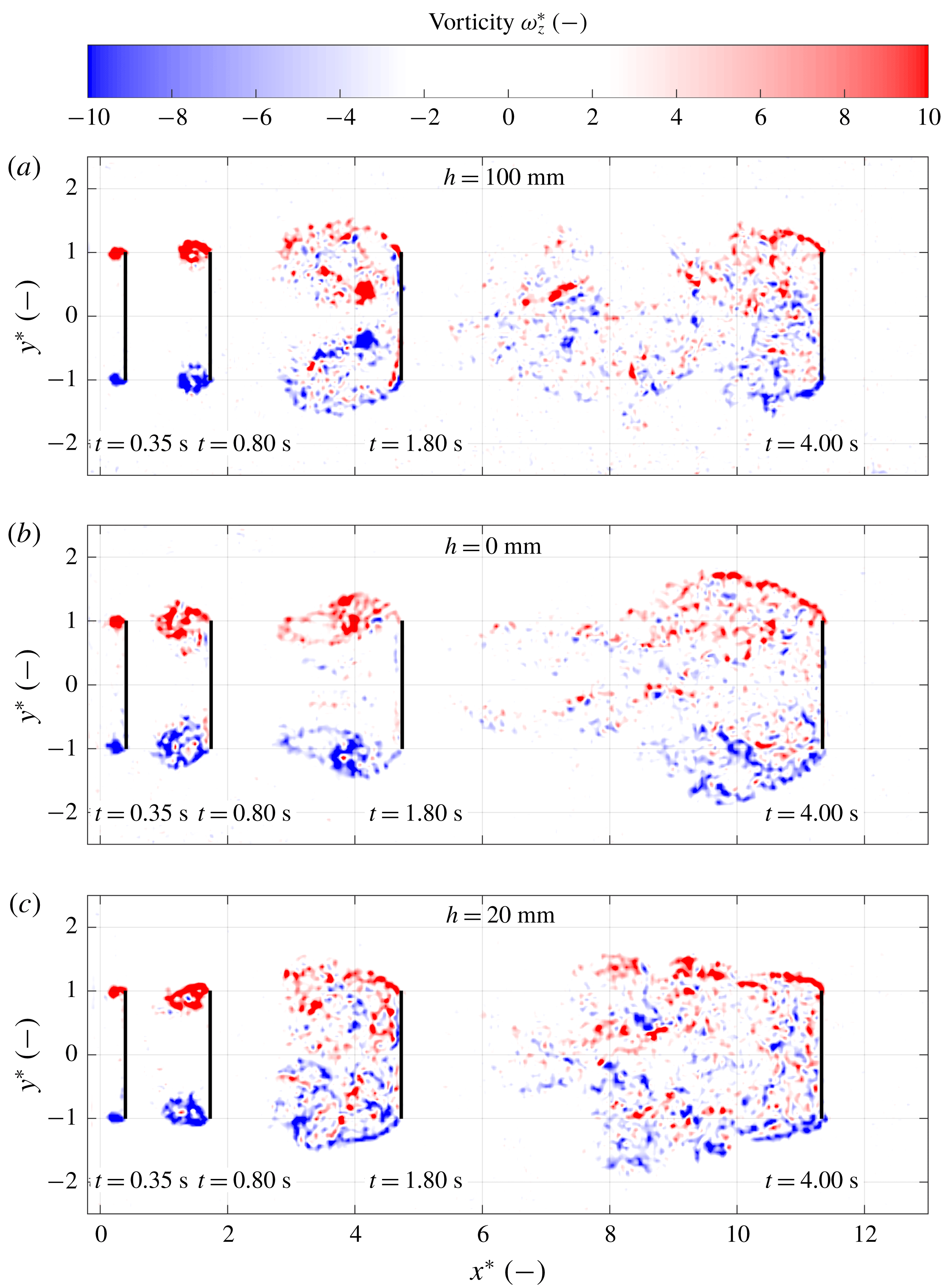
Figure 16 shows the vorticity $\unicode[STIX]{x1D714}_{z}^{\ast }$
for all three selected depths for different times
$\unicode[STIX]{x1D714}_{z}^{\ast }$
for all three selected depths for different times $t$
, including the instances in time corresponding to those of the flow visualisations in figure 8. Note that a movie of the time evolution of all three cases, side-by-side, is available in the supplemental material (movie 4). For all three cases the formation of a vortex pair during the acceleration phase, i.e. up to
$t$
, including the instances in time corresponding to those of the flow visualisations in figure 8. Note that a movie of the time evolution of all three cases, side-by-side, is available in the supplemental material (movie 4). For all three cases the formation of a vortex pair during the acceleration phase, i.e. up to $t=0.35$
s appears very similar and matches to the cross-section of the vortex ring at the mid-plane of the plate, as shown in figure 8(a,d,g).
$t=0.35$
s appears very similar and matches to the cross-section of the vortex ring at the mid-plane of the plate, as shown in figure 8(a,d,g).
When the plate approaches $x^{\ast }=2$
at
$x^{\ast }=2$
at $t=0.80$
s the wakes start to differ. The vortex pair of the case
$t=0.80$
s the wakes start to differ. The vortex pair of the case $h=100$
mm is still very close and concentrated to the mid-plane of the plate, as is also seen in figure 8(b), while in both cases
$h=100$
mm is still very close and concentrated to the mid-plane of the plate, as is also seen in figure 8(b), while in both cases $h=0$
and
$h=0$
and $h=20$
mm the vortices start to travel away from the plate and become less defined. This matches the behaviour shown in figure 8(e,h).
$h=20$
mm the vortices start to travel away from the plate and become less defined. This matches the behaviour shown in figure 8(e,h).
For $t^{\ast }>4$
at
$t^{\ast }>4$
at $t=1.80$
s, i.e. well into the transition phase, each wake becomes very distinct. The vortices in the case of
$t=1.80$
s, i.e. well into the transition phase, each wake becomes very distinct. The vortices in the case of $h=100$
mm are still attached to the plate, but have moved inwards, i.e. the vortex ring has contracted in the
$h=100$
mm are still attached to the plate, but have moved inwards, i.e. the vortex ring has contracted in the $y$
-direction, and two large circulation zones around the vortex pair are formed in which the secondary vortices formed in the shear layer are shed. During this contraction process the two highly concentrated circulation zones move from the plate edge towards the centre of the plate creating a strong and large low pressure zone. We speculate that this is associated with a characteristic peak in the drag force at
$y$
-direction, and two large circulation zones around the vortex pair are formed in which the secondary vortices formed in the shear layer are shed. During this contraction process the two highly concentrated circulation zones move from the plate edge towards the centre of the plate creating a strong and large low pressure zone. We speculate that this is associated with a characteristic peak in the drag force at $t^{\ast }=2.8$
, e.g. shown as peak 1 in figure 12(d). At the same plate depth
$t^{\ast }=2.8$
, e.g. shown as peak 1 in figure 12(d). At the same plate depth $h=100$
mm, some time after the situation at
$h=100$
mm, some time after the situation at $t=1.80$
s shown in figure 16, the two well-defined vortices trailing closely behind the centre of the plate touch and collapse which may be associated with a second peak in the drag force signal, e.g. shown as peak 2 in figure 12(d). In the other two cases the circulation zones are not so concentrated. The large circulation zones in the case of
$t=1.80$
s shown in figure 16, the two well-defined vortices trailing closely behind the centre of the plate touch and collapse which may be associated with a second peak in the drag force signal, e.g. shown as peak 2 in figure 12(d). In the other two cases the circulation zones are not so concentrated. The large circulation zones in the case of $h=0$
mm stretch in streamwise direction and detach, while the circulation zones in the case of
$h=0$
mm stretch in streamwise direction and detach, while the circulation zones in the case of $h=20$
mm already disintegrate into a chaotic wake.
$h=20$
mm already disintegrate into a chaotic wake.
Well into the steady phase, i.e. at $t=4.00$
s where the plate passes
$t=4.00$
s where the plate passes $x^{\ast }=11.5$
, the wakes also look very distinct. The case of
$x^{\ast }=11.5$
, the wakes also look very distinct. The case of $h=100$
mm shows an asymmetric wake with what appears to be an oscillating tail, which is a well-known phenomenon for steady flow over a plate (Fage & Johansen Reference Fage and Johansen1927; Hemmati, Wood & Martinuzzi Reference Hemmati, Wood and Martinuzzi2016). The cases
$h=100$
mm shows an asymmetric wake with what appears to be an oscillating tail, which is a well-known phenomenon for steady flow over a plate (Fage & Johansen Reference Fage and Johansen1927; Hemmati, Wood & Martinuzzi Reference Hemmati, Wood and Martinuzzi2016). The cases $h=0$
mm and
$h=0$
mm and $h=20$
mm both show a symmetric wake of similar size, but the latter has a large amount of vorticity very close to the plate which, we conjecture, (partially) explains the maximum steady-phase drag
$h=20$
mm both show a symmetric wake of similar size, but the latter has a large amount of vorticity very close to the plate which, we conjecture, (partially) explains the maximum steady-phase drag $C_{D}$
found for this plate depth (
$C_{D}$
found for this plate depth ( $h=20$
mm), see figure 4. Also, we note the difference in wake angle. Whereas the wake angles in the vertical plane are quite similar, clearly visible in the visualisation (figure 8), the wake angles in the horizontal plane differ substantially. It appears that the case with the highest drag (
$h=20$
mm), see figure 4. Also, we note the difference in wake angle. Whereas the wake angles in the vertical plane are quite similar, clearly visible in the visualisation (figure 8), the wake angles in the horizontal plane differ substantially. It appears that the case with the highest drag ( $h=20$
mm) has the smallest wake angle, while the case with the lowest drag (
$h=20$
mm) has the smallest wake angle, while the case with the lowest drag ( $h=0$
mm) has the largest wake angle, see figure 16.
$h=0$
mm) has the largest wake angle, see figure 16.
Dimensionless vorticity $\unicode[STIX]{x1D714}_{z}^{\ast }$
for different instances in time
$\unicode[STIX]{x1D714}_{z}^{\ast }$
for different instances in time $t$
at a selected depth of
$t$
at a selected depth of $h=100$
mm. The flow behaviour appears to be very similar for both realisations. Only in the steady phase
$h=100$
mm. The flow behaviour appears to be very similar for both realisations. Only in the steady phase $t=4.00$
s the tail of the wake sweeps up in one realisation (a) and down in the other (b) which matches the characteristic oscillating wake as was already observed by Fage & Johansen (Reference Fage and Johansen1927). The dashed line around the outer border shows the area of integration
$t=4.00$
s the tail of the wake sweeps up in one realisation (a) and down in the other (b) which matches the characteristic oscillating wake as was already observed by Fage & Johansen (Reference Fage and Johansen1927). The dashed line around the outer border shows the area of integration $S$
for which the circulation is obtained. The symmetry line through
$S$
for which the circulation is obtained. The symmetry line through $y^{\ast }=0$
is also marked and shows the dividing line between integration surfaces
$y^{\ast }=0$
is also marked and shows the dividing line between integration surfaces $S_{-}$
and
$S_{-}$
and $S_{+}$
.
$S_{+}$
.
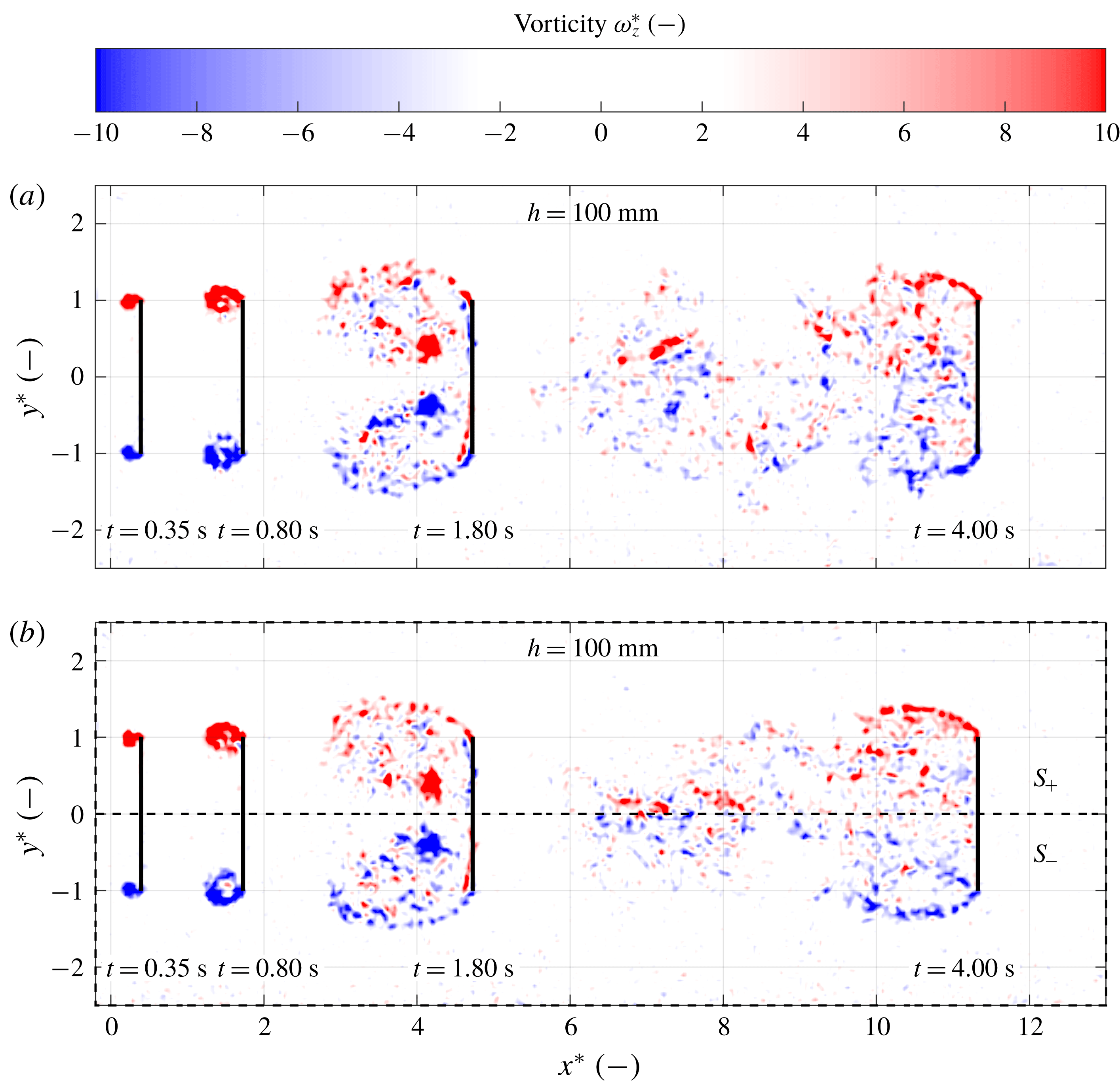
To test the reproducibility of the PIV measurements, the experiments were performed three times for each plate depth $h$
. The realisations at the same depth are highly reproducible. Only at a plate depth of
$h$
. The realisations at the same depth are highly reproducible. Only at a plate depth of $h=100$
mm around
$h=100$
mm around $t=4.00$
s a clear difference between realisations is found, as shown in figure 17. The two different realisations are very similar except that the tail of the wake of the realisation shown in the top figure sweeps up, while in the figure at the bottom the tail sweeps down. A sweeping tail which starts in an arbitrary direction shows that this is not due to imperfections in the experimental set-up.
$t=4.00$
s a clear difference between realisations is found, as shown in figure 17. The two different realisations are very similar except that the tail of the wake of the realisation shown in the top figure sweeps up, while in the figure at the bottom the tail sweeps down. A sweeping tail which starts in an arbitrary direction shows that this is not due to imperfections in the experimental set-up.
3.10 Circulation and shedding events
In previous studies (Gharib et al.
Reference Gharib, Rambod and Shariff1998; Ringuette et al.
Reference Ringuette, Milano and Gharib2007) the total circulation $\unicode[STIX]{x1D6E4}$
was used to identify vortex shedding events. The total circulation is obtained by integrating the local vorticity over a surface, i.e.
$\unicode[STIX]{x1D6E4}$
was used to identify vortex shedding events. The total circulation is obtained by integrating the local vorticity over a surface, i.e.
 $$\begin{eqnarray}\unicode[STIX]{x1D6E4}=\int _{S}\unicode[STIX]{x1D714}_{z}\,\text{d}S.\end{eqnarray}$$
The dimensionless circulation $\unicode[STIX]{x1D6E4}^{\ast }$
is obtained by integration of
$\unicode[STIX]{x1D6E4}^{\ast }$
is obtained by integration of $\unicode[STIX]{x1D714}_{z}^{\ast }$
(defined in (3.11)) over the dimensionless flow field area
$\unicode[STIX]{x1D714}_{z}^{\ast }$
(defined in (3.11)) over the dimensionless flow field area $S$
formed by the entire range of
$S$
formed by the entire range of $x^{\ast }$
and
$x^{\ast }$
and $y^{\ast }$
. Kelvin’s circulation theorem states that integration over
$y^{\ast }$
. Kelvin’s circulation theorem states that integration over $S$
should yield a net circulation of
$S$
should yield a net circulation of $\unicode[STIX]{x1D6E4}^{\ast }=0$
if the integration boundary is along a material contour (Cohen & Kundu Reference Cohen and Kundu2007) as long as the flow is symmetric, i.e. produces no lift. The flow conditions for the theorem to hold, i.e. inviscid and barotropic flow, are fulfilled by choosing the material contour along the boundaries of the field of view of the PIV measurements, where the flow is at rest, indicated by the dashed line along the outer border in figure 17(b).
$\unicode[STIX]{x1D6E4}^{\ast }=0$
if the integration boundary is along a material contour (Cohen & Kundu Reference Cohen and Kundu2007) as long as the flow is symmetric, i.e. produces no lift. The flow conditions for the theorem to hold, i.e. inviscid and barotropic flow, are fulfilled by choosing the material contour along the boundaries of the field of view of the PIV measurements, where the flow is at rest, indicated by the dashed line along the outer border in figure 17(b).
The grey lines in figure 18 show the circulation $\unicode[STIX]{x1D6E4}^{\ast }$
as a function of the formation time
$\unicode[STIX]{x1D6E4}^{\ast }$
as a function of the formation time $t^{\ast }$
for
$t^{\ast }$
for $h=100$
, 0 and 20 mm, respectively. For all three plate depths, throughout each realisation, the total circulation
$h=100$
, 0 and 20 mm, respectively. For all three plate depths, throughout each realisation, the total circulation $\unicode[STIX]{x1D6E4}^{\ast }$
is very close to zero. However, at the intervals
$\unicode[STIX]{x1D6E4}^{\ast }$
is very close to zero. However, at the intervals $4.8<t^{\ast }<6$
and
$4.8<t^{\ast }<6$
and $t^{\ast }>9.4$
the measured circulation
$t^{\ast }>9.4$
the measured circulation $\unicode[STIX]{x1D6E4}^{\ast }$
does not appear to be conserved perfectly. This deviation between measurements and theory is explained by measurement errors (random noise). The non-zero total circulation based on
$\unicode[STIX]{x1D6E4}^{\ast }$
does not appear to be conserved perfectly. This deviation between measurements and theory is explained by measurement errors (random noise). The non-zero total circulation based on $S$
coincides with the stitching seams of the flow field as indicated by the dashed vertical lines in figure 18, showing that the flow field is not stitched seamlessly. In the case of
$S$
coincides with the stitching seams of the flow field as indicated by the dashed vertical lines in figure 18, showing that the flow field is not stitched seamlessly. In the case of $h=20$
mm the trailing vortex, as shown in figure 8(i), might cause large out of plane motion which also affects the measurement accuracy (Adrian & Westerweel Reference Adrian and Westerweel2011).
$h=20$
mm the trailing vortex, as shown in figure 8(i), might cause large out of plane motion which also affects the measurement accuracy (Adrian & Westerweel Reference Adrian and Westerweel2011).
As was noted before, the flow field maintains symmetrical well into the steady phase. To quantify this symmetry and to identify vortex shedding events, the flow field area $S$
is subdivided into two areas along the symmetry plane of the plate,
$S$
is subdivided into two areas along the symmetry plane of the plate, $S_{-}$
and
$S_{-}$
and $S_{+}$
, corresponding to
$S_{+}$
, corresponding to $y^{\ast }<0$
and
$y^{\ast }<0$
and $y^{\ast }>0$
, respectively (figure 17
b). Integration of the vorticity over each area results in the total circulation
$y^{\ast }>0$
, respectively (figure 17
b). Integration of the vorticity over each area results in the total circulation $\unicode[STIX]{x1D6E4}^{\ast }$
of each region, as shown in figure 18. Throughout all runs, i.e. for all cases and each realisation, the circulation is
$\unicode[STIX]{x1D6E4}^{\ast }$
of each region, as shown in figure 18. Throughout all runs, i.e. for all cases and each realisation, the circulation is $\unicode[STIX]{x1D6E4}^{\ast }>0$
for area
$\unicode[STIX]{x1D6E4}^{\ast }>0$
for area $S_{+}$
and
$S_{+}$
and $\unicode[STIX]{x1D6E4}^{\ast }<0$
for area
$\unicode[STIX]{x1D6E4}^{\ast }<0$
for area $S_{-}$
. Clearly, for
$S_{-}$
. Clearly, for $t^{\ast }<4.8$
all cases behave very similar with virtually no difference between realisations.
$t^{\ast }<4.8$
all cases behave very similar with virtually no difference between realisations.
The ability of the total circulation $\unicode[STIX]{x1D6E4}^{\ast }$
to identify vortex shedding becomes clear at
$\unicode[STIX]{x1D6E4}^{\ast }$
to identify vortex shedding becomes clear at $6<t^{\ast }<8$
for the case
$6<t^{\ast }<8$
for the case $h=100$
mm, where a temporary decrease in circulation occurs due to the two touching vortices as described in § 3.9. The same mechanism is described by Ringuette et al. (Reference Ringuette, Milano and Gharib2007) as an ‘inward’ pinch-off. They obtained a circulation profile with ‘inward’ pinch-off occurring at
$h=100$
mm, where a temporary decrease in circulation occurs due to the two touching vortices as described in § 3.9. The same mechanism is described by Ringuette et al. (Reference Ringuette, Milano and Gharib2007) as an ‘inward’ pinch-off. They obtained a circulation profile with ‘inward’ pinch-off occurring at $t^{\ast }\approx 4$
where in this study the pinch-off occurs at
$t^{\ast }\approx 4$
where in this study the pinch-off occurs at $t^{\ast }\approx 6$
. Their circulation profile is very similar in shape compared to the one presented here, even though the plate in their work pierces the surface and has different dimensions, i.e.
$t^{\ast }\approx 6$
. Their circulation profile is very similar in shape compared to the one presented here, even though the plate in their work pierces the surface and has different dimensions, i.e. $l_{a}=0.127$
m and height
$l_{a}=0.127$
m and height $l_{b}=0.0635$
m. In the case of
$l_{b}=0.0635$
m. In the case of $h=20$
mm an ordinary pinch-off occurs at
$h=20$
mm an ordinary pinch-off occurs at $t^{\ast }=8$
, identified by an interval of constant total circulation (Gharib et al.
Reference Gharib, Rambod and Shariff1998). For the case of
$t^{\ast }=8$
, identified by an interval of constant total circulation (Gharib et al.
Reference Gharib, Rambod and Shariff1998). For the case of $h=0$
mm shedding events were not observed in the vorticity field, nor were indications of those events present in the measured circulation.
$h=0$
mm shedding events were not observed in the vorticity field, nor were indications of those events present in the measured circulation.
Apart from identifying shedding events, the total circulation in $S^{-}$
and
$S^{-}$
and $S^{+}$
in figure 18 quantitatively shows that the experiments are well reproducible, although the circulation increasingly deviates for larger times
$S^{+}$
in figure 18 quantitatively shows that the experiments are well reproducible, although the circulation increasingly deviates for larger times $t^{\ast }$
. This deviation is smallest for the case
$t^{\ast }$
. This deviation is smallest for the case $h=0$
mm, which suggests that the free surface suppresses this deviation.
$h=0$
mm, which suggests that the free surface suppresses this deviation.
The grey lines show the circulation $\unicode[STIX]{x1D6E4}^{\ast }$
as a function of formation time
$\unicode[STIX]{x1D6E4}^{\ast }$
as a function of formation time $t^{\ast }$
based on the total flow field
$t^{\ast }$
based on the total flow field $S$
, while the black lines show the circulation
$S$
, while the black lines show the circulation $\unicode[STIX]{x1D6E4}^{\ast }$
based on the top half-area
$\unicode[STIX]{x1D6E4}^{\ast }$
based on the top half-area $S_{+}$
and bottom half-area
$S_{+}$
and bottom half-area $S_{-}$
as indicated in the figure. The three different realisations at each depth are represented by different line styles. A break-up event in the case
$S_{-}$
as indicated in the figure. The three different realisations at each depth are represented by different line styles. A break-up event in the case $h=100$
mm is clearly visible around
$h=100$
mm is clearly visible around $t^{\ast }=7$
, as is a pinch-off event around
$t^{\ast }=7$
, as is a pinch-off event around $t^{\ast }=8$
in the case
$t^{\ast }=8$
in the case $h=20$
mm. The vertical dashed lines show the stitching seams of the flow field.
$h=20$
mm. The vertical dashed lines show the stitching seams of the flow field.

4 Discussion and conclusion
In this study the flow around plates accelerating at $a$
towards a fixed plate velocity
$a$
towards a fixed plate velocity $V$
at various submerged depths
$V$
at various submerged depths $h$
is investigated using measurement techniques that complement each other. The drag force on the plate as a function of time is measured, the three-dimensional flow around the plate is visualised using hydrogen bubble flow visualisation and the two-dimensional flow field in the horizontal mid-plane of the plate is measured quantitatively using PIV from which the vorticity
$h$
is investigated using measurement techniques that complement each other. The drag force on the plate as a function of time is measured, the three-dimensional flow around the plate is visualised using hydrogen bubble flow visualisation and the two-dimensional flow field in the horizontal mid-plane of the plate is measured quantitatively using PIV from which the vorticity $\unicode[STIX]{x1D714}_{z}$
and total circulation
$\unicode[STIX]{x1D714}_{z}$
and total circulation $\unicode[STIX]{x1D6E4}$
are derived.
$\unicode[STIX]{x1D6E4}$
are derived.
The steady-phase drag coefficient is found to have a remarkable peak at a plate depth of $h=20$
mm, i.e. 45 % higher than the drag at the surface (
$h=20$
mm, i.e. 45 % higher than the drag at the surface ( $h=0$
mm) and 20 % higher than when the plate is submerged one plate height
$h=0$
mm) and 20 % higher than when the plate is submerged one plate height $h=100$
mm (
$h=100$
mm ( $h/l_{b}=1$
). The definition of the steady phase
$h/l_{b}=1$
). The definition of the steady phase $t>3.4$
s (
$t>3.4$
s ( $t^{\ast }>10$
) based on the measured force signals matches with the flow visualisations (figure 8, and movies available in the supplemental material as movie 1, movie 2 and movie 3) and the vorticity fields (figure 16, supplemental material movie 4). The drag force during the acceleration phase appears to be very complex but is shown to be well behaved:
$t^{\ast }>10$
) based on the measured force signals matches with the flow visualisations (figure 8, and movies available in the supplemental material as movie 1, movie 2 and movie 3) and the vorticity fields (figure 16, supplemental material movie 4). The drag force during the acceleration phase appears to be very complex but is shown to be well behaved:
 $$\begin{eqnarray}F_{x}(t)=\underbrace{m_{p}a(t)}_{F_{mp}}+\underbrace{\frac{1}{2}\unicode[STIX]{x1D70C}V(t)^{2}C_{D}A}_{F_{CD}}+\underbrace{\frac{\text{d}m_{h}}{\text{d}t}a(t)(t-t_{sr})+m_{h(Yu)}a}_{F_{mh}}.\end{eqnarray}$$
We showed that the force due to added mass $F_{mh}$
is constant for small
$F_{mh}$
is constant for small $t^{\ast }$
and matches results reported by Yu (Reference Yu1945). For
$t^{\ast }$
and matches results reported by Yu (Reference Yu1945). For $t^{\ast }$
the expression is expanded based on an entrainment rate
$t^{\ast }$
the expression is expanded based on an entrainment rate $\text{d}m_{h}/\text{d}t$
that models an increasing mass in the wake of the plate. This entrainment rate appears to be independent of velocity and almost constant for different accelerations
$\text{d}m_{h}/\text{d}t$
that models an increasing mass in the wake of the plate. This entrainment rate appears to be independent of velocity and almost constant for different accelerations $a$
. We conclude that the entrainment rate is an important parameter to predict the maximum hydrodynamic forces on plate-like geometries and that the entrainment rate is strongly enhanced by the vicinity of a free surface; at the surface, for a plate depth of
$a$
. We conclude that the entrainment rate is an important parameter to predict the maximum hydrodynamic forces on plate-like geometries and that the entrainment rate is strongly enhanced by the vicinity of a free surface; at the surface, for a plate depth of $h=0$
mm, the entrainment rate is found to be 50 % larger than for plate depths of
$h=0$
mm, the entrainment rate is found to be 50 % larger than for plate depths of $h=20$
and
$h=20$
and $h=100$
mm. During the transition phase the force decreases for the case of
$h=100$
mm. During the transition phase the force decreases for the case of $h=100$
mm along a distinct profile with two large peaks, peak 1 and peak 2. These are associated with vortex shedding events visible in both the visualisations, the vorticity field and the circulation profiles. For different velocities these peaks perfectly align in time by use of the formation time
$h=100$
mm along a distinct profile with two large peaks, peak 1 and peak 2. These are associated with vortex shedding events visible in both the visualisations, the vorticity field and the circulation profiles. For different velocities these peaks perfectly align in time by use of the formation time $t^{\ast }$
, as shown in figure 12(d). Also, the force due to hydrodynamic mass during the transition phase appears to scale with the formation time as
$t^{\ast }$
, as shown in figure 12(d). Also, the force due to hydrodynamic mass during the transition phase appears to scale with the formation time as $F_{mh}\sim 1/{t^{\ast }}^{2}$
, where
$F_{mh}\sim 1/{t^{\ast }}^{2}$
, where $t^{\ast }$
is essentially the distance travelled by the plate. This scaling is hypothesised to be due to the plate moving away from the shed starting vortex. A scaling argument supports this hypothesis and in the visualisations it is shown that a large vortex in the vertical plane is indeed shed.
$t^{\ast }$
is essentially the distance travelled by the plate. This scaling is hypothesised to be due to the plate moving away from the shed starting vortex. A scaling argument supports this hypothesis and in the visualisations it is shown that a large vortex in the vertical plane is indeed shed.
The motivation for this study stems from (competitive) rowing. During rowing the oar blade moves along a complicated cycloid path not only producing drag, but also lift, making a comparison with an accelerating flat plate along a straight path somewhat complicated. However, during the start of a rowing match the oar blade accelerates from rest along a more linear path and travels ${\approx}10$
times the blade height before the next stroke (
${\approx}10$
times the blade height before the next stroke ( $t^{\ast }\approx 10$
); very much like the flat plate in this study. It stands to reason that for a rowing oar blade an optimal depth exists, which is a trade-off between decreasing entrainment rate and increasing steady-phase drag with increasing depth
$t^{\ast }\approx 10$
); very much like the flat plate in this study. It stands to reason that for a rowing oar blade an optimal depth exists, which is a trade-off between decreasing entrainment rate and increasing steady-phase drag with increasing depth $h$
. Also the starting technique where athletes use several short strokes to achieve cruising speed as fast as possible seems hydrodynamically advantageous. The drag on the plate is at its maximum while accelerating and up to the steady phase a history force is present. This means that while accelerating the plate and during the transition phase the generation of drag force is more efficient, i.e. the plate produces a higher force at an equal or lower velocity than in the steady phase. During the acceleration phase this effect is strongest, so with several short strokes the oar blade spends a longer time in the acceleration phase and early transition phase, and would thus be more efficient.
$h$
. Also the starting technique where athletes use several short strokes to achieve cruising speed as fast as possible seems hydrodynamically advantageous. The drag on the plate is at its maximum while accelerating and up to the steady phase a history force is present. This means that while accelerating the plate and during the transition phase the generation of drag force is more efficient, i.e. the plate produces a higher force at an equal or lower velocity than in the steady phase. During the acceleration phase this effect is strongest, so with several short strokes the oar blade spends a longer time in the acceleration phase and early transition phase, and would thus be more efficient.
Acknowledgements
This work is part of the research programme ‘Optimisation of propulsion in and over water’ with project number 12186, which is (partly) financed by the Netherlands Organisation for Scientific Research (NWO).
Supplementary movies
Supplementary movies are available at https://doi.org/10.1017/jfm.2019.102.
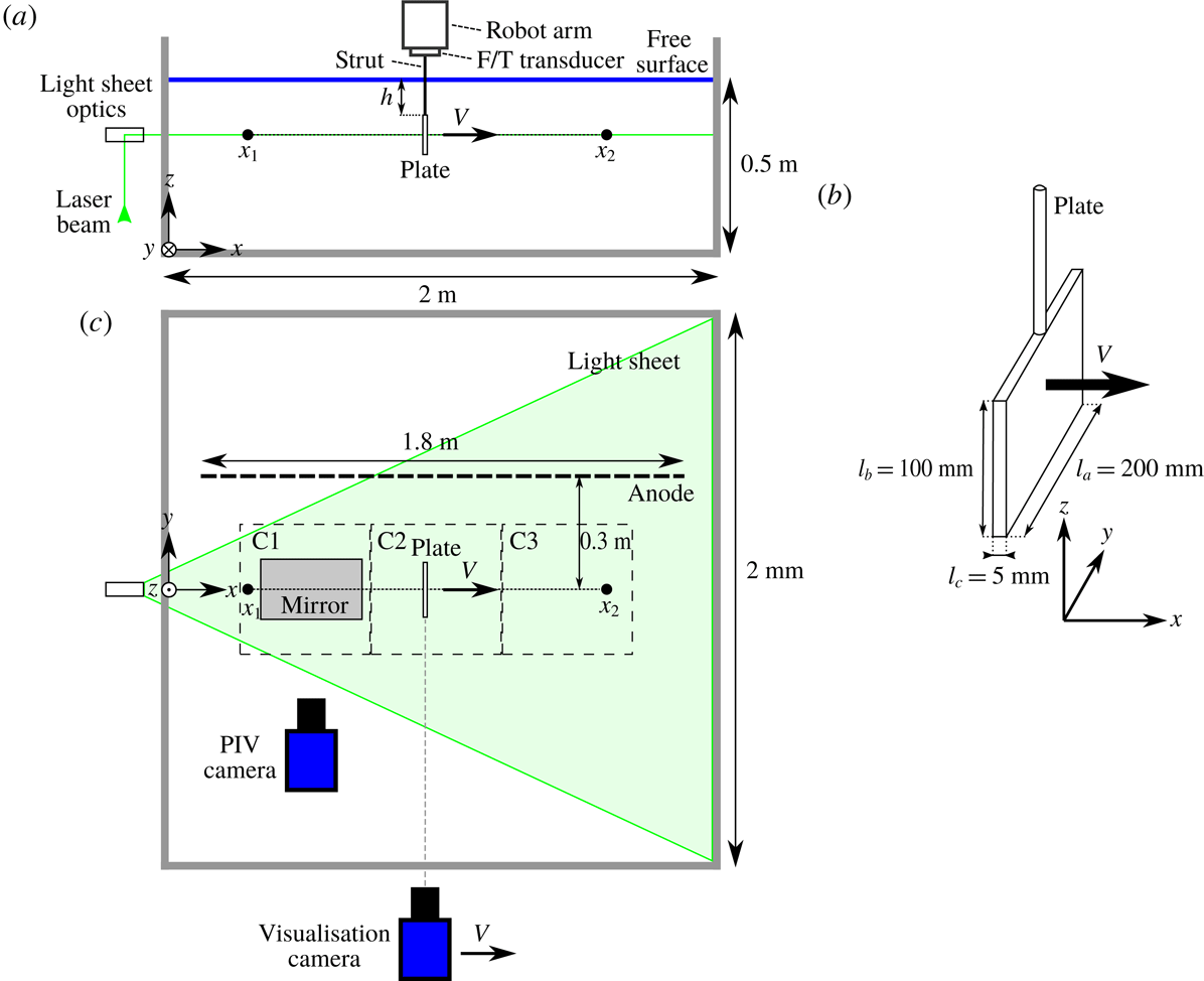

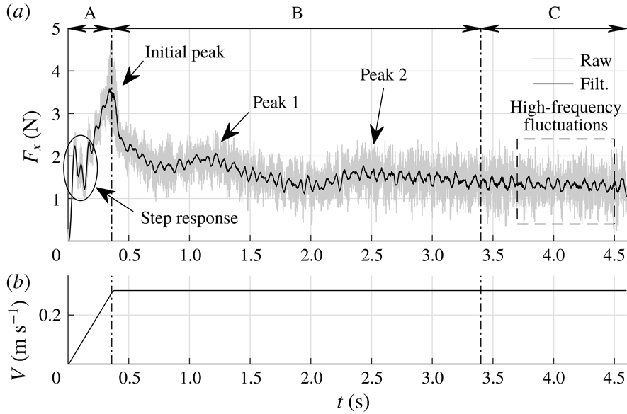

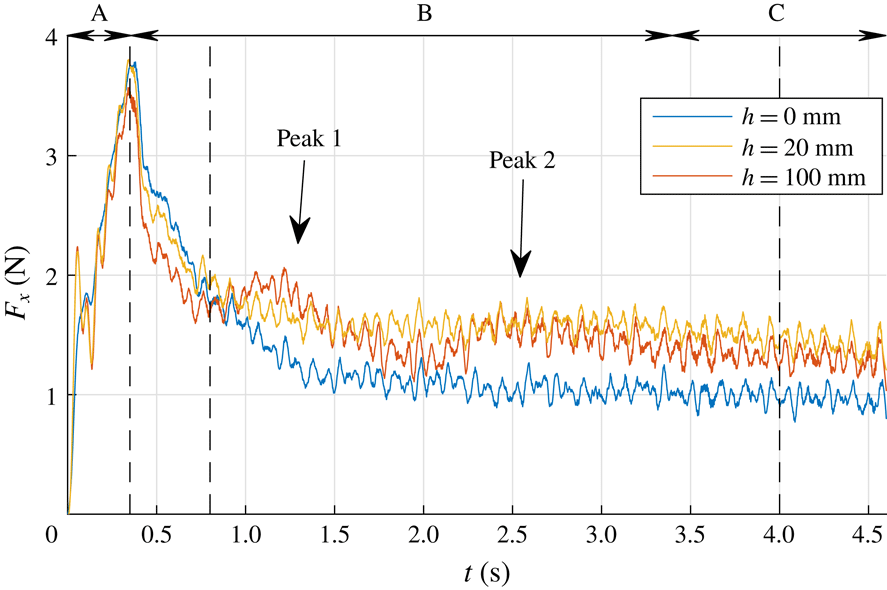
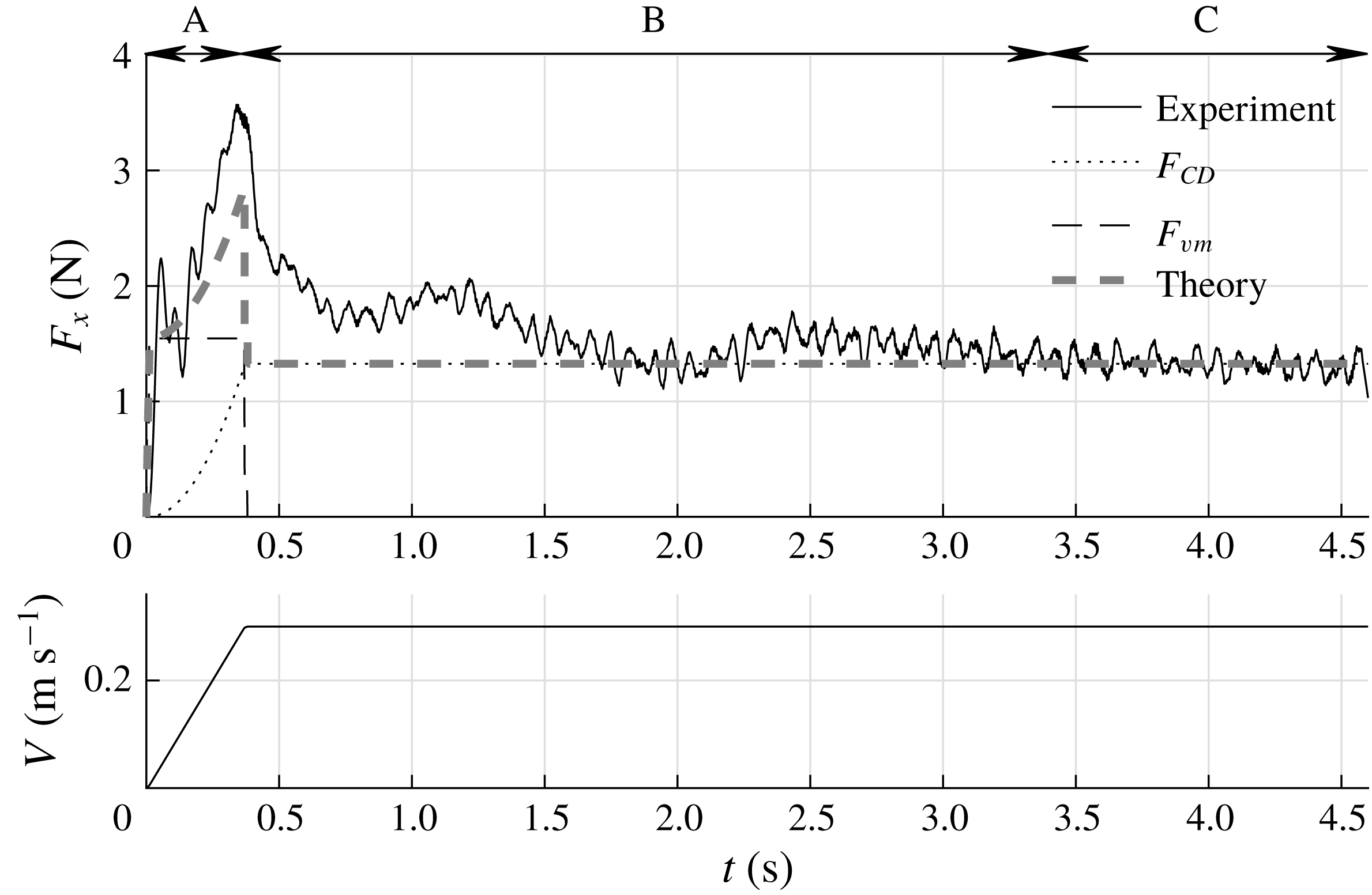
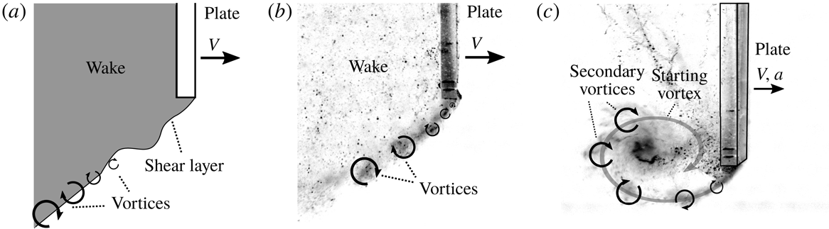

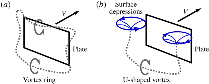
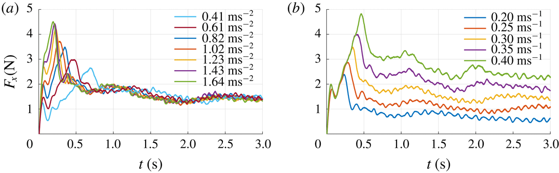

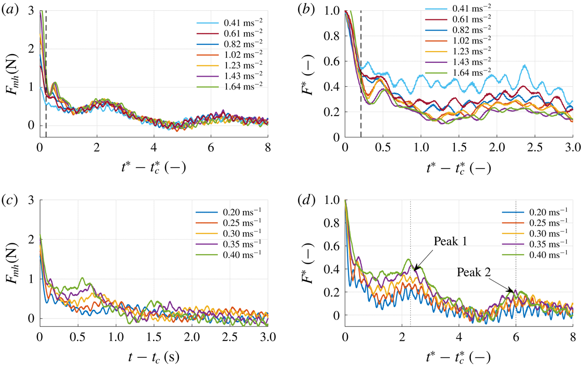

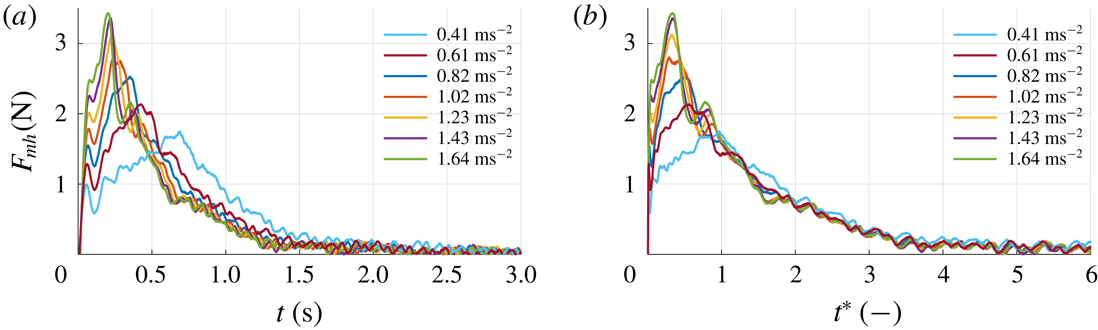

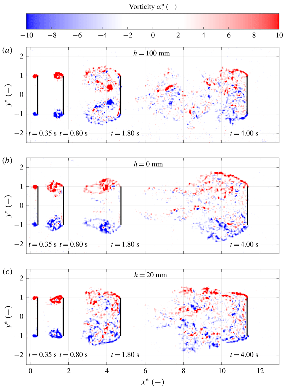

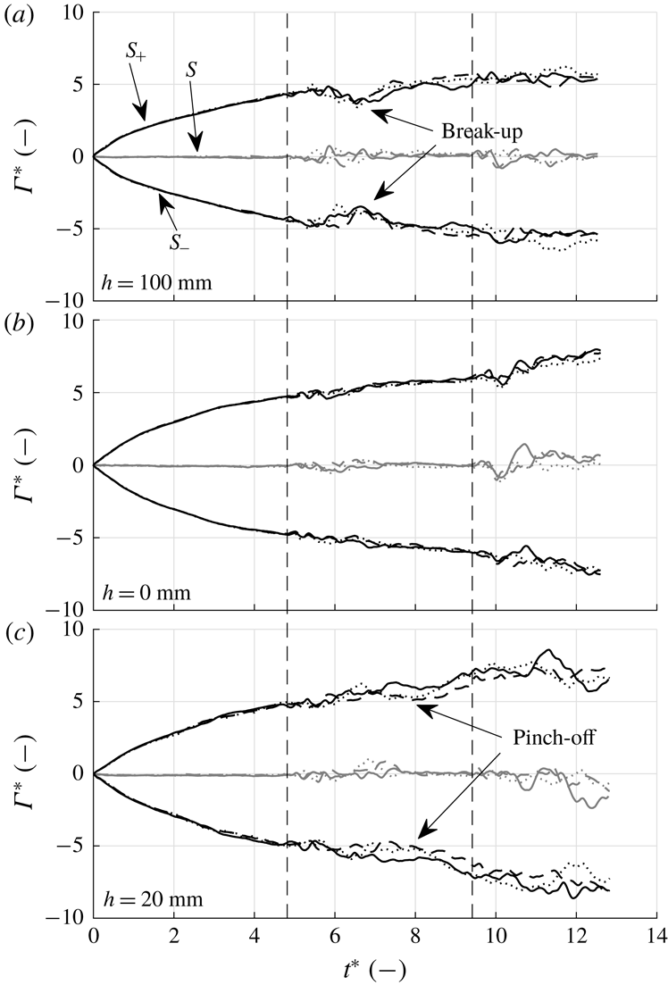


 Open access

