







1. Introduction
In Moffatt & Kimura (Reference Moffatt and Kimura2019a) (hereafter Reference Moffatt and KimuraMK19a), we have derived the following dimensionless equations describing the approach and early-stage interaction of two initially circular vortex tubes (radius  $R$, circulations $\pm \varGamma$) inclined to a plane of symmetry at angles $\pm \alpha$ (figure 1a; lengths and time $\tau \ge 0$ are made dimensionless relative to $R$ and $R^2/\varGamma$; the fluid is assumed incompressible):
 \begin{equation} \frac{\text{d} s}{\text{d}{ \tau}}={-}\frac{\kappa\cos\alpha}{4{\rm \pi}}\varLambda, \quad \frac{\text{d} \kappa}{\text{d}{\tau}}=\frac{\kappa\cos\alpha\sin\alpha}{4{\rm \pi} {s}^2},\quad \frac{\text{d} \delta^2}{\text{d}{\tau}}=\epsilon -\frac{\kappa\cos\alpha}{4{\rm \pi} {s}} \delta^{2}, \end{equation}
where  $\varLambda (\tau )=\log (s/\delta )+\beta _1$ and (for vortices of Gaussian core structure) $\beta _1 =0.4417$. Here, $2 s(\tau )$, $\kappa (\tau )$ and $\delta (\tau )$ represent, respectively, the separation of the vortices, the curvature and the vortex core radii at their nearest points of approach (the ‘tipping points’). The term $\epsilon \equiv \nu /\varGamma \equiv R_{\varGamma }^{-1}$ is the inverse of the vortex Reynolds number, and represents the natural tendency of $\delta ^{2}$ to increase due to viscous diffusion; this is counteracted by the term $-({\kappa \cos \alpha }/{4{\rm \pi} {s}}) \delta ^{2}$, which represents the effect of vortex stretching. Arguments were given in Reference Moffatt and KimuraMK19a to justify the particular choice of angle $\alpha ={\rm \pi} /4$, but it was recognised in the conclusions that smaller values of $\alpha$ should also be considered.
(a) Sketch of the initial vortex tube configuration. (b) Vorticity profiles represented as the sum of Gaussians  $\omega /\omega _{0}=\exp [-(x-s)^{2}/4\delta ^2]- \exp [-(x+s)^{2}/4\delta ^2]$ for fixed $\delta \ (=1)$ and $s/\delta =7$ (black), $5$ (blue), $3$ (green) and $1$ (red). For $s/\delta \gtrsim 5$ the vortices are essentially non-overlapping, but, as $s/\delta$ decreases below $5$, the overlap becomes increasingly significant.

Equations (1.1a–c) were derived under the assumptions
 \begin{equation} 0< \delta(\tau) \ll s(\tau) \ll \kappa(\tau)^{{-}1},\quad\text{with} \ \kappa(0)=1, \end{equation}
and were assumed to be valid only for so long as these conditions are satisfied. However, it became apparent that these severe inequalities fail to persist when time  $\tau$ gets very near to a critical finite ‘singularity time’ $\tau _c$; as this time approaches, $s \sim \delta$, so that the initially circular vortex cross-sections become deformed, and (if $\epsilon >0$) viscous reconnection occurs. We attempted to describe the reconnection process by introducing a fourth variable $\gamma (\tau )$ representing the proportion of the circulation $\varGamma$ that is reconnected at time $\tau$ (Moffatt & Kimura Reference Moffatt and Kimura2019b, Reference Moffatt and Kimura2020). However, direct numerical simulation (DNS) for the same configuration (Yao & Hussain Reference Yao and Hussain2020) has indicated that the resulting fourth-order dynamical system does not correctly capture the complexities of the reconnection process.
Since the vorticity is localised (here exponentially small outside a finite domain) and has Gaussian structure within the tubes, the fluid velocity  ${\boldsymbol u}({\boldsymbol x}, 0)$ is analytic and of order $r^{-3}$ at infinity. The energy of the vortex tube configuration at time $\tau =0$ is of order $R \varGamma ^{2}\log [R/\delta (0)]$, and is finite since $\delta (0)>0$. Similarly, all Sobolev norms (including enstrophy, of order $\varGamma ^{2} R/\delta (0)^{2}$) are finite since $\delta (0)>0$ (for related discussion for the case of a periodic domain, see Kang, Yun & Protas (Reference Kang, Yun and Protas2020)).
The first of the inequalities (1.2),  $s(\tau ) \gg \delta (\tau )$, ensured that the vortex cores remain compact and non-overlapping, allowing use of the Biot–Savart law in deriving (1.1a). Figure 1(b) shows a section of a vortex pair $\omega /\omega _{0}=\exp [-(x-s)^{2}/4\delta ^2]\,-\, $ $\exp [-(x+s)^{2}/4\delta ^2]$ for several values of $s/\delta$; the overlap of the cores becomes significant only when $s/\delta \lesssim 5$. The condition $s(\tau ) \gg \delta (\tau )$ is evidently too restrictive: what is really required is that
 \begin{equation} \exp[{-}s^{2}/4\delta^{2}] \ll 1. \end{equation}
When  $s/\delta =\{3,4,5, 6,\ldots \}$, then $\exp [-s^{2}/4\delta ^{2}] \approx \{0.11,0.02, 0.002, 0.0001,\ldots \}$, respectively. Hence (1.3) is in effect satisfied provided
 \begin{equation} s /\delta \ge k_{1},\quad \text{where}\ k_{1} \ \text{is a constant} \gtrsim 5. \end{equation}
 Similarly, the second of the inequalities (1.2),  $\kappa ^{-1}\gg s(\tau )$, ensures that the interaction between the two vortices is localised within an O $(s)$ neighbourhood of the tipping points, and this persists for so long as
 \begin{equation} (s\kappa)^{{-}1}\ge k_{2}, \end{equation}
where, again,  $k_{2}$ is a constant somewhat greater than unity. We shall find that, if we require that the limiting equalities, $s /\delta = k_{1}$ in (1.4) and $(s\kappa )^{-1}= k_{2}$ in (1.5), be simultaneously satisfied, then, for sufficiently small $\delta (0)/s(0)$, $k_{2}$ is actually determined as a function of $k_{1}$ (see (3.8) and figure 3b); this functional relationship provides a value of $k_{2}$ that increases monotonically from 3.89 to 4.96 as $k_{1}$ increases from 5 to 10.
The inequalities (1.4) and (1.5) define what we may describe as phase I of the interaction process, which is of finite duration,  $T$ say. Phase II is then the subsequent period when these inequalities are not satisfied, and when strong deformation of the vortex cores occurs. Our purpose in the present paper is to determine the maximum amplification of the axial vorticity $\omega _{0}=\varGamma /4{\rm \pi} \delta ^2$ that may be attained during phase I when both inequalities (1.4) and (1.5) remain satisfied; in this respect, our aim parallels that of Kang et al. (Reference Kang, Yun and Protas2020). (For the purpose of illustration, we shall generally adopt the values $k_{1}=5$ and $k_{2}=3.89$, so that then, as explained above, the constraints $s /\delta \ge k_{1}$ and $(s\kappa )^{-1}\ge k_{2}$ are precisely compatible; the main conclusions do not, however, depend on these choices.)
In a related paper, Morrison & Kimura (Reference Morrison and Kimura2020) have proved that, when  $\epsilon =0$ (the Euler limit), the system (1.1a–c) is a ‘non-canonical’ Hamiltonian system with two invariants, the Hamiltonian $H(s, \delta )$ (independent of $\kappa$) and a Casimir $C(s,\kappa,\delta )$. (These invariants are closely associated with the results (2.8) and (3.6) of the present paper; see Appendix A.) The solution trajectories are then curves of intersection of the surfaces $H= {\rm const.}$ and $C= {\rm const.}$ in the three-dimensional space of the variables $\{s,\kappa,\delta \}$. On each such trajectory, $s$ and $\kappa$ are determined as functions of $\delta$, so that (1.1c) provides a quadrature determining $\delta (\tau )$. By this means, a general solution was obtained, revealing a finite-time singularity with Leray scaling $s\sim (\tau _{c}-\tau )^{1/2}$, $\delta \sim (\tau _{c}-\tau )^{1/2}$ and $\kappa \sim (\tau _{c}-\tau )^{-1/2}$ (and confirming the asymptotic analysis in § 8 of Reference Moffatt and KimuraMK19a). The problem, however, is that $\delta /s$ increases to near unity as $\tau \rightarrow \tau _{c}$ (actually to $\exp (\beta _{1}-1/2) \approx 0.943$), so that the condition (1.3) no longer holds good as the singularity is approached. Some flattening of the vortex-core cross-sections is inevitable, invalidating the basis on which the system (1.1a–c) was obtained. The DNS of McKeown et al. (Reference McKeown, Ostilla-Monico, Pumir, Brenner and Rubenstein2018) and of Ostilla-Monica et al. (Reference Ostilla-Monica, McKeown, Brenner, Rubenstein and Pumir2021), albeit at finite Reynolds number, indicated that this flattening process can be quite severe, in effect converting tubes to sheets, which are then subject to elliptic instabilities, and/or Kelvin–Helmholtz instabilities (as earlier suggested by Brenner, Hormoz & Pumir (Reference Brenner, Hormoz and Pumir2016)).
Similar behaviour was found in the DNS of Yao & Hussain (Reference Yao and Hussain2020), who also reported that, at a vortex Reynolds number of 4000 (and with  $s(0)=0.1$ and $\delta (0)=0.01$), the maximum vorticity did not increase by more than a factor of about 1.6 during the whole interaction and reconnection process. This surprising result may be contrasted with the result of simulations based on the Biot–Savart law for vortex filaments, as shown in figure 1 of Reference Moffatt and KimuraMK19a, which indicated a singularity ( $s\rightarrow 0,\ \kappa \rightarrow \infty$) as $\tau \rightarrow \tau _{c}$. Here, we seek to understand this contrasting behaviour by choosing $z\equiv \delta (0)/s(0)$ very small (to approach the vanishingly small value implicit in the above use of the Biot–Savart law for vortex filaments), and by considering the asymptotic behaviour as $z \rightarrow 0$. (We here ignore the fact that, on ever decreasing microscopic scales, the continuum description of the fluid must ultimately fail.)
To recap, it is apparent that there are two phases to the vortex interaction process: phase I, of finite duration  $T$, when the cores do not significantly overlap, but the axes of both vortex rings are deformed by the interaction, with associated stretching; and phase II, when the cores do impinge on each other, with consequent strong core deformation and (if $\epsilon >0$) the onset of reconnection. Phase I is defined by the inequalities (1.4) and (1.5), and the analysis of the present paper is restricted to this phase. We make no assertion concerning phase II, for which DNS is an indispensable mode of investigation (as, for example, in the paper of Kerr (Reference Kerr2018), who has used DNS to study the phase II reconnection process for two prototypical vortex tube configurations (antiparallel and trefoil knot)).
2. Solution in the Euler limit  $\epsilon =0$

Here we first provide a straightforward derivation of the exact solution, obtained by Morrison & Kimura (Reference Morrison and Kimura2020), of the dynamical system (1.1a–c) in the Euler limit. When  $\epsilon =0$, we note first that (1.1a–c) imply that $\kappa (\tau )$ is monotonically increasing and (with $s > \delta$) $s(\tau )$ and $\delta (\tau )$ are monotonically decreasing. Moreover, these equations give
 \begin{equation} \frac{\text{d}\delta}{\text{d}s} =\frac{\text{d}\delta/\text{d}\tau}{\text{d}s/\text{d}\tau} =\frac{\delta}{2\varLambda s}. \end{equation}
Here it is convenient to introduce variables
 \begin{equation} \sigma\equiv s(\tau)/s_{0} <1\quad \text{and}\quad \lambda\equiv \delta(\tau)/\delta_{0} <1,\quad \text{for} \ \tau >0, \end{equation}
where  $s_{0}=s(0)$ and $\delta _{0}=\delta (0)$ (with $\kappa _{0}=\kappa (0)=1$). Equations (1.1a–c) become
 \begin{equation} \frac{\text{d} \sigma}{\text{d}{ \tau}}={-}\frac{\kappa\cos\alpha}{4{\rm \pi} s_{0}}\varLambda, \quad \frac{\text{d} \kappa}{\text{d}{\tau}}=\frac{\kappa\cos\alpha\sin\alpha}{4{\rm \pi} s_{0}^{2}\sigma^{2}},\quad \frac{\text{d} \lambda^2}{\text{d}{\tau}}=\frac{\epsilon}{\delta_{0}^{2}} -\frac{\kappa\cos\alpha}{4{\rm \pi} {s_{0}\sigma}}\lambda^{2}, \end{equation}
and the logarithmic term  $\varLambda$ becomes
 \begin{equation} \varLambda(\sigma,\lambda,z)=\log(\sigma/\lambda)-\log{z}+\beta_{1}, \quad\text{where}\ z=\delta_{0}/s_{0}\ll 1. \end{equation}
Equation (2.1) becomes
 \begin{equation} \frac{\text{d}\lambda}{\lambda} =\frac{\text{d}\sigma}{2\varLambda(\sigma,\lambda,z)\sigma}, \quad \text{or equivalently} \quad \text{d}\log{\lambda}=\frac{\text{d}\log{\sigma}}{2\varLambda(\sigma,\lambda,z)}, \end{equation}
with ‘initial’ condition  $\lambda =1$ when $\sigma = 1$. The condition $s\gg \delta$ becomes $\sigma /\lambda \gg z$. As argued above, it seems reasonable to adopt $5z$ as the value of $\sigma /\lambda$ above which the vortex cores do not significantly overlap and so remain effectively circular, i.e. the inequality (1.3) may then be deemed to be satisfied. (We choose this level for illustrative purposes only; any level $k_{1} z$, with $k_{1} \gtrsim 3$ and constant in the limit $z\rightarrow 0$, could be chosen.)
Now, defining  $L=\log {\lambda }$, $S=\log {\sigma }$ and $Z=\beta _{1}-\log {z}=\log [e^{\beta _{1}}/z]$, and using (2.4), we obtain the linear equation
 \begin{equation} \text{d}S/\text{d}L = 2(S-L+Z),\quad \text{with initial condition}\ S(0)=0. \end{equation}
The solution is
 \begin{equation} S(L)= L+\tfrac{1}{2}(1-2Z)(1-\text{e}^{2L}), \end{equation}
or, returning to the variables  $\{\sigma, \lambda \}$,
 \begin{equation} \sigma = \lambda q^{\lambda^{2}-1}\quad\text{where}\ q=\text{e}^{\beta_{1}-1/2}/z\approx 0.943/z. \end{equation}
Here, note immediately that  $\sigma /\lambda \rightarrow q^{-1}= 1.060 z$ when $\lambda \rightarrow 0$, so that, as recognised by Reference Moffatt and KimuraMK19a, the condition $\sigma /\lambda \gg z$ is not satisfied in this limit. (Note further that $\sigma /\lambda = {\rm const.}$ if $q=1$, i.e. $z=0.943$; this is the special situation for which Morrison & Kimura's Hamiltonian $H(s,\delta )=0$.)
The less restrictive condition  $\sigma /\lambda \gtrsim k_{1}z$ with $k_{1}\gtrsim 3$ now becomes
 \begin{equation} q^{\lambda^{2}-1}\gtrsim k_{1}z, \end{equation}
or equivalently
 \begin{equation} \lambda^{2}\gtrsim \lambda_{m}^{2}=1+\frac{\log[k_{1}z]}{\log{q}} \sim\frac{\log{k_{1}}-0.059}{\log[1/z]}\quad \text{as}\ z\rightarrow 0. \end{equation}
(The condition  $\lambda \gtrsim \lambda _{m}(z)$ now determines the duration of phase I of the evolution.) With the choice $k_{1}=5$ ( $\log {k_{1}}=1.609$), (2.10) becomes
 \begin{equation} \lambda_{m}^{2}\sim \frac{1.550}{\log[1/z]}\quad \text{as}\ z\rightarrow 0. \end{equation}
The corresponding asymptotic amplification of vorticity at the tipping points is then
 \begin{equation} \mathcal{A}_{\omega}\equiv \omega_{max}/\omega_{0}\equiv 1/\lambda_{m}^2 \sim 0.645 \log[1/z], \end{equation}
where  $\omega _{0}$ now represents the initial axial vorticity magnitude in each vortex tube. Thus an arbitrarily large amplification of vorticity $\mathcal {A}_{\omega }$ can be achieved in phase I (in principle if not in practice) by choosing $z$ sufficiently small, specifically by choosing
 \begin{equation} z\sim\text{e}^{{-}1.550 \mathcal{A}_{\omega}}. \end{equation}
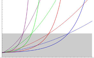
 Figure 2(a) shows plots of  $\sigma /\lambda z\ (=s/\delta )$ versus $\lambda$ for four values of $z$ decreasing from $10^{-5}$ to $10^{-50}$. The black line at level 5 intersects these curves at the values $\lambda =\lambda _{m}(z)$ given by (2.11) and indicated by the vertical dashed lines, showing the very slow decrease of $\lambda _{m}(z)$ as $z\rightarrow 0$ (for example, $\lambda _{m}(10^{-5})\approx 0.367, \lambda _{m}(10^{-50})\approx 0.116$). The model loses validity where the curves lie in the shaded phase II region below the level $\sigma /\lambda z=5$.
(a) Plot of  $\sigma /\lambda z\ (= s/\delta )$ versus $\lambda$ in the range $0\le \lambda \le 0.5$ for $z=10^{-5}$ (blue), $10^{-10}$ (red), $10^{-25}$ (green) and $10^{-50}$ (purple). The horizontal line at the level $k_{1}=5$ separates phase I (unshaded, above) from phase II (shaded, below), and intersects the curves at $\lambda =\lambda _{m}(z)$ for each $z$ (as marked by the vertical dashed lines). Note the very slow decrease of $\lambda _{m}(z)$ with decreasing $z$. All these curves asymptote to 1.060 as $\lambda \rightarrow 0$. (b) The same with corresponding dashed curves of $(s_{0}\kappa \sigma )^{-1}\ [=(s\kappa )^{-1}]$ superposed (with $s_{0}=0.02$ and $\alpha ={\rm \pi} /4$). These dashed curves are scaled by the factor $k_{1}/k_{2}=5/3.89\approx 1.29$, bringing them into approximate coincidence with the solid curves at the level 5. This shows that, when $k_{1}=5$, both inequalities (1.4) and (1.5) are simultaneously satisfied with the choice $k_{2}= 3.89$. The dashed curves asymptote to $1.29/\sqrt {2}\approx 0.912$ as $\lambda \rightarrow 0$.

3. Evaluation of $\sigma \kappa$ as a function of $\lambda$


We also need to satisfy the inequality  $(s_{0}\sigma \kappa )^{-1} > k_{2}$ (with $k_{2}=3.89$ corresponding to $k_{1}=5$); $s_{0}$ must also be chosen to be suitably small. It is now convenient to calculate
 \begin{equation} \frac{\text{d}\kappa}{\text{d}\lambda} =\frac{\text{d}\kappa/\text{d}\tau}{\text{d}\lambda/\text{d}\tau} ={-}\frac{2\sin{\alpha}}{s_{0}\sigma\lambda}. \end{equation}
Here we may use (2.8), so that, with  $q=0.943/z$ as before,
 \begin{equation} \frac{\text{d}\lambda}{\lambda^{2}q^{\,\lambda^{2}-1}}={-}\frac{s_{0}}{2 \sin{\alpha}}\,\text{d}\kappa,\quad\text{and so}\quad \kappa-1=\frac{2 \sin{\alpha}}{s_{0}}I(q,\lambda), \end{equation}
where, using the initial condition  $\kappa =1$ when $\lambda =1$,
 \begin{equation} I(q,\lambda)=\int_{\lambda}^{1} \frac{\text{d}\lambda_{1}}{\lambda_{1}^{2}q^{\lambda_{1}^{2}-1}} = \lambda^{{-}1}q^{1-\lambda^{2}}-1+q\sqrt{{\rm \pi} \log{q}} [\text{erf}(\lambda\sqrt{\log{q}})-\text{erf}(\sqrt{\log{q}})]. \end{equation}
The function  $I(q,\lambda )$ has the asymptotic behaviour
 \begin{equation} I(q,\lambda) \sim \frac{q}{\lambda} - [1+q\sqrt{{\rm \pi} \log{q}}\,\text{erf}(\sqrt{\log{q}})]+\text{O}(\lambda)\quad\text{as} \lambda\rightarrow 0, \end{equation}
so that, from (3.2),
 \begin{equation} \kappa \sim \left(\frac{2q\sin{\alpha}}{s_{0}}\right) \frac{1}{\lambda}+\text{O}(1)\quad\text{as} \lambda\rightarrow 0. \end{equation}
It follows further from (3.2) that
 \begin{equation} s\kappa\equiv s_{0}\sigma\kappa = \lambda q^{\lambda^{2}-1}[s_{0}+2 \sin{\alpha}I(q,\lambda)]. \end{equation}
This expression approaches the limit  $2 \sin {\alpha }$ as $\lambda \rightarrow 0$. We require that $\lambda$ be restricted to the range for which $(s_{0}\sigma \kappa )^{-1} > k_{2}$. The relevant portions of the curves of $1.29 (s_{0}\sigma \kappa )^{-1}$ are shown, dashed, in figure 2(b) for $\alpha ={\rm \pi} /4$, $s_{0}=0.02$, and for the same four values of $z$ as in figure 2(a). The scaling factor $1.29=k_{1}/k_{2}$ corresponds to the choices $k_{1}=5,\ k_{2}=3.89$, for which the limiting equalities in (1.4) and (1.5) are simultaneously satisfied.
As recognised by Morrison & Kimura (Reference Morrison and Kimura2020), if  $\alpha \le {\rm \pi}/6$, the limit $2\sin {\alpha }$ for $(s\kappa )$ satisfies $(s\kappa )|_{\lim }\le 1$, supporting the possibility of a fluid-dynamical singularity as $\tau \rightarrow \tau _{c}$. However, the corresponding limit $(\delta /s)|_{\lim }=0.943$ does not depend on $\alpha$, and is too large to provide any confidence that both the underlying conditions (1.2) of the model are adequately satisfied right up until the instant at which the potential singularity might be attained.
If, instead of the level 5, we choose any level  $k_{1}\gtrsim 3$ for the minimum allowed value of $s/\delta$, then, for given $z$, (2.10) determines $k_{1}$ as a function of $\lambda _{m}$. We may then obtain the corresponding minimum allowed value $k_{2}$ for $(s_0 \sigma \kappa )^{-1}$, as a function of the same $\lambda _{m}$. In this way, with $q(z)=0.943/z$, we find
 \begin{equation} k_{1}(\lambda_{m},z)=z^{{-}1}q(z)^{\lambda_{m}^{2}-1},\quad k_{2}(\lambda_{m},z)=\lambda_{m}^{{-}1}q(z)^{1-\lambda_{m}^{2}} [s_{0}+2\sin{\alpha}\,I(q(z),\lambda_{m})]^{{-}1}. \end{equation}
 Figure 3(a) shows the functions  $k_{1}(\lambda _{m},z)$ and $k_{2}(\lambda _{m},z)$ as functions of $\lambda _{m}$ for $s_{0}=0.02,\ \alpha ={\rm \pi} /4$, and for $z=10^{-5},\ 10^{-10}$, $10^{-25}$ and $10^{-50}$.
(a) Plot of  $k_{1}(\lambda _{m},z)$ (solid) and $k_{2}(\lambda _{m},z)$ (dashed) for $\alpha ={\rm \pi} /4$ and $z=10^{-5}$ (blue), $10^{-10}$ (red), $10^{-25}$ (green) and $10^{-50}$ (purple). The dotted line is at the level 3.08 where the curves cross. (b) Plot of the asymptotic function $k_{2}(k_{1})$ for $s_{0}=0.02$, $\alpha ={\rm \pi} /4$, in the range $3\le k_{1}\le 10$.

If  $\lambda _{m}$ is now eliminated from (3.7) the dependence of $k_{2}$ on $k_{1}$ may be obtained. The asymptotic behaviour of this relationship as $z\rightarrow 0$, i.e. as $q(z)\rightarrow \infty$, is, to good approximation,
 \begin{equation} k_{2}\sim 2^{{-}1/2} \{1+k_{1}\sqrt{{\rm \pi}\log{k_{1}}} (\text{erf}[\sqrt{\log{k_{1}}}]-1)\}^{{-}1} \quad \text{as}\ z\rightarrow 0. \end{equation}
This asymptotic function  $k_{2}(k_{1})$ is shown in figure 3(b) for the range $3\le k_{1}\le 10$. We note that $k_{2}(3)\approx 3.08$, $k_{2}(5)\approx 3.89$ and $k_{2}(10)\approx 4.96$, and that, in this range of $k_{1}$, one has $0.49 < k_{2}/k_{1}<1.1$. Since this ratio is of order unity, the implication is that, if the first required inequality $s/\delta > k_{1}$ is satisfied, then so is the second $(s \kappa )^{-1} > k_{2}$, with $k_{2}$ chosen to satisfy (3.8). It is sufficient then to focus just on the requirement $s/\delta \equiv \sigma /\lambda z > k_{1}$.
4. Determination of $\lambda (\tau )$

From (1.1c), with  $\epsilon =0$, we now have
 \begin{equation} \frac{\text{d} \lambda}{\text{d}{\tau}}={-}\left(\frac{\cos\alpha}{8{\rm \pi} s_{0}}\right)\left[\frac{\kappa(\lambda)}{ \sigma(\lambda)}\right] \lambda ,\quad\text{with}\ \lambda(0)=1, \end{equation}
where  $\kappa (\lambda )$ and $\sigma (\lambda )$ are now given by (3.2) and (2.8), respectively. This equation shows that $\lambda (\tau )$ does indeed decrease monotonically to zero, and determination of $\lambda (\tau )$ is now reduced to a quadrature that does not admit evaluation in terms of known functions. However, we require the behaviour only for so long as $\lambda >\lambda _{m}(z)$, and this can be obtained by numerical integration. Figure 4 shows the results of such integration (using Mathematica) for $\alpha ={\rm \pi} /4,\ s_{0}= 0.02$ and $z= 10^{-5}$ (blue), $10^{-8}$ (red) and $10^{-11}$ (purple). Each computation stalls just before the singularity is reached; for smaller $z$ we cannot be sure of the accuracy of the integration process.
The function  $\lambda (\tau )$ obtained by numerical integration of (4.1) with initial condition $\lambda (0)=1$; $\alpha ={\rm \pi} /4,\ s_{0}=0.02$ and $z= 10^{-5}$ (blue), $10^{-8}$ (red) and $10^{-11}$ (purple). The vertical dashed lines indicate the ‘singularity time’ $\tau _{c}(z)$ in each case. The horizontal dotted lines indicate the corresponding levels $\lambda =\lambda _{m}(z)$, as given by (2.10) with $k_{1}=5$, below which the conditions of the model lose validity.

We can, however, obtain the asymptotic behaviour of  $\lambda (\tau )$ as $\tau \rightarrow \tau _{c}$ by using the results $\sigma \sim \lambda /q$ (from (2.8)) and $\kappa \sim 2q\sin {\alpha }/(s_{0}\lambda )$ (from (3.5)) as $\lambda \rightarrow 0$. With these asymptotic results, and with $\epsilon =0$, (2.3c) gives
 \begin{equation} \frac{\text{d}\lambda^{2}}{\text{d}\tau}\sim{-}m^{2},\quad\text{where}\ m=\frac{q}{2s_{0}}\left(\frac{\sin{2\alpha}}{\rm \pi}\right)^{1/2}, \end{equation}
so that  $\lambda \sim m(\tau _{c}-\tau )^{1/2}$ and so
 \begin{equation} \sigma\sim \frac{m}{q}(\tau_{c}-\tau)^{1/2},\quad \kappa\sim \frac{2q\sin{\alpha}}{s_{0}m}(\tau_{c}-\tau)^{{-}1/2},\quad \text{as} \tau\rightarrow\tau_c, \end{equation}
thus recovering Leray scaling.
We emphasise, however, that these asymptotic results apply in the grey area of figure 2(b), and that our present model loses validity as the curves descend into this area. (Recall that the minimum value  $\lambda =\lambda _{m}(z)$ at which the underlying approximation (1.3) fails to persist is given explicitly by (2.10), and asymptotically for small $z$ by (2.11).) The derivation of the results (4.3) is nevertheless of interest in that (3.1) involves the ‘stretched variable’ $\kappa (\lambda )$ which is asymptotically proportional to $\lambda ^{-1}$ and so tends to infinity as $\tau _{c}-\tau \rightarrow 0$. Use of a stretched variable is the key ingredient of the technique developed by Mulungye, Lucas & Bustamante (Reference Mulungye, Lucas and Bustamante2015) in a more general context for the resolution of finite-time singularities.
Note that the impending singularity times  $\tau =\tau _{c}(z)$, indicated by the vertical lines in figure 4, actually decrease with decreasing $z$; this is because the two vortices propagate towards each other more rapidly as $\delta _{0}$ decreases (due to the logarithmic factor), other parameters being fixed. The levels $\lambda =\lambda _{m}(z)$ below which the model loses validity, indicated by the horizontal dotted lines, also decrease with decreasing $z$, as already evident over the much wider range of $z$ in figure 2(a,b). Note that the levels $\lambda _{m}(z)$ are reached only when the ‘plunge to zero’ is already well under way.
5. Inclusion of viscosity $\epsilon >0$

It has been proved by Constantin (Reference Constantin1986, § 1) that if, for given initial conditions of finite suitably defined Sobolev norm  $\|{\cdot }\|$, a solution ${\boldsymbol u}({\boldsymbol x},t)$ of the Euler equations remains smooth throughout a time interval $0< t< T$, then, for sufficiently small viscosity $\nu$, the solution ${\boldsymbol v}({\boldsymbol x},t)$ of the Navier–Stokes equations satisfying the same initial conditions also remains smooth for the same time interval; and moreover that $\|{\boldsymbol v} ({\boldsymbol x},t)-{\boldsymbol u}({\boldsymbol x},t)\|={O}(\nu )$ for $0< t< T$ as $\nu \rightarrow 0$. In our present situation, we have a solution of (1.1a–c) when $\epsilon \ (\equiv \nu /\varGamma ) =0$ that is smooth up to the finite time $T$ by which $\lambda$ has decreased to $\lambda _{m}(z)$. In the light of Constantin's theorem, we may therefore anticipate the existence of a similarly smooth solution for sufficiently small $\epsilon >0$ during the same finite time interval.
Returning to (1.1a–c), it is obvious that if, for so long as  $\lambda >\lambda _{m}(z)$, $\epsilon$ satisfies the inequality
 \begin{equation} \epsilon \ll \frac{\kappa\cos{\alpha}}{4{\rm \pi} s}\delta^{2} = \frac{z^{2} s_{0}\kappa\lambda^2 \cos{\alpha} }{4{\rm \pi}\sigma}, \end{equation}
then inclusion of viscosity should have little effect on  $\lambda _{m}$, and so on the maximum vorticity amplification factor $\mathcal {A}_{\omega }=\lambda _{m}^{-2}$ that can be attained for given $z$. We can now seek to determine just how large a Reynolds number $R_{\varGamma }=\epsilon ^{-1}$ will be sufficient for the result (2.12) to remain valid. Note first that $\sigma /\lambda$ decreases monotonically as $\lambda$ decreases from 1 to 0, and so does $(\kappa \sigma )^{-1}$, provided $s_{0}$ is sufficiently small, specifically provided
 \begin{equation} s_{0}<2 \sin{\alpha}/(1+2\log{q}). \end{equation}
It follows that, under this condition, the expression on the right of (5.1) increases monotonically as  $\lambda$ decreases, and is minimal at the initial instant when $\lambda =\sigma =\kappa =1$. The inequality (5.1) at this instant is
 \begin{equation} \epsilon\ll \epsilon_{c}=z^2 s_{0}\cos{\alpha}/(4{\rm \pi}) \end{equation}
(cf. (8.8) of Reference Moffatt and KimuraMK19a) and, if this holds at  $\tau =0$, then a fortiori (5.1) holds throughout the subsequent evolution until $\lambda =\lambda _{m}$. Thus, to achieve a vorticity amplification factor $\mathcal {A}_{\omega }$ , it is sufficient that $z$ should satisfy (2.13) and, in addition, that $R_{\varGamma }\equiv \epsilon ^{-1}$ should satisfy the inequality
 \begin{equation} R_{\varGamma} \gg 4{\rm \pi} \sec{\alpha} \, s_{0}^{{-}1}\text{e}^{3.10\mathcal{A}_{\omega}}. \end{equation}
 Figure 5(a) shows the effect of increasing  $\epsilon$ from zero for the case $\alpha ={\rm \pi} /4,\ z=10^{-5}$, first to the critical level $\epsilon _{c}$, then to multiples of $\epsilon _{c}$ up to $200\epsilon _{c}$; we here choose $s_{0}=0.02$, which safely satisfies the inequality (5.2). Remarkably, the function $\lambda (\tau )$ is negligibly affected by viscosity in the range $0<\epsilon <\epsilon _{c}$. This means that if $R_{\varGamma }\gtrsim R_{\varGamma c} \equiv \epsilon _{c}^{-1}$, then the amplification factor $\mathcal {A}_{\omega }$ is likewise negligibly affected by viscosity.
Effect of viscosity for  $\alpha ={\rm \pi} /4,\ s_{0}=0.02$ and $z= 10^{-5}$. (a) The function $\lambda (\tau )$ obtained by numerical integration of the full dynamical system (1.1a–c) for $\epsilon = 0$ (blue), $\epsilon =\epsilon _{c}$ (red), almost indistinguishable from the blue curve, $\epsilon =50 \epsilon _{c}$ (green), $\epsilon =100 \epsilon _{c}$ (purple) and $\epsilon =200 \epsilon _{c}$ (black), where $\epsilon _{c}$ is given by (5.3). In the last three cases, although $\lambda$ increases initially, it ultimately falls to zero at a ‘singularity time’ $\tau _{c}(\epsilon )$ just a little greater than that found for $\epsilon =0$. (b) Evolution of $\lambda (\tau )$ (blue) and $z \lambda (\tau )/\sigma (\tau )$ (red) very near to $\tau _{c}$ for the case $\epsilon =0$; the red curve crosses the level $1/5=0.2$ at $\tau =\tau _{m}$, and $\lambda (\tau _{m})=\lambda _{m}$. The model is valid only for $\tau <\tau _{m}$ (phase I). (c) The same for $\epsilon =4\epsilon _{c}$, for which the value of $\lambda _{m}$ is only slightly increased. (d) The same for $\epsilon =100\epsilon _{c}$, for which the increase in $\lambda _{m}$ (and corresponding decrease in $\mathcal {A}_{\omega })$ is now substantial.

For  $\epsilon >\epsilon _{c}$, the function $\lambda (\tau )$ initially rises (due to conventional viscous diffusion of the vortex cores), but ultimately plunges to zero just as for the case $\epsilon =0$. However, the value $\lambda _{m}$ at which the model loses validity increases with $\epsilon$, and eventually exceeds unity, so that then $\mathcal {A}_{\omega }<1$, i.e. there is then no amplification of maximum vorticity. Figure 5(b) shows how this effect may be quantified; this shows a late stage of evolution for the case $\epsilon =0$. The red curve shows $z \lambda (\tau )/\sigma (\tau )$, which crosses the level $1/5=0.2$ at time $\tau =\tau _{m}$, say. We can be confident that the model is valid up to this time. The function $\lambda (\tau )$ is decreasing and $\lambda (\tau _{m})=\lambda _{m}$. This graphical procedure determines $\lambda _{m}=0.368$ (just as given by the formula (2.10) with $z=10^{-5}$) with correspondingly $\mathcal {A}_{\omega }=1/\lambda _{m}^{2}= 7.38$.
The same procedure can be carried out for any  $\epsilon$. Figure 5(c) shows the result for $\epsilon =4 \epsilon _{c}$; here, $\lambda _{m}$ has increased by only a small amount to 0.389 ( $\mathcal {A}_{\omega }= 6.61$). Figure 5(d) shows the result for $\epsilon =100 \epsilon _{c}$; here, as might be expected, the effect is more marked (note the change of scale in the ordinate): $\lambda _{m}=0.752$ ( $\mathcal {A}_{\omega }=\lambda _{m}^{-2}= 1.77)$. For $\epsilon =200 \epsilon _{c}$, $\lambda _{m}=1.015$ ( $\mathcal {A}_{\omega }= 0.97)$, and vorticity is suppressed rather than amplified. These results are all for $z=10^{-5}$; for smaller $z$, one may expect a corresponding reduction in the values of $\lambda _{m}$.
The above results help us to understand the very modest vorticity amplification found in the DNS of Yao & Hussain (Reference Yao and Hussain2020), who, with the choices  $s_{0}=0.1,\ \delta _{0}=0.01$ (so $z=0.1$), found an amplification factor of only ${\sim }1.6$ at Reynolds number $R_{\varGamma }=4000$. With these values of $s_{0}$ and $z$, (2.10) gives $\mathcal {A}_{\omega }=1.45$ if $k_{1}=5$ (and 1.69 if $k_{1}=4$), and (5.4) gives a sufficiently large Reynolds number of about 16 000. Figure 7(a) of Yao & Hussain (Reference Yao and Hussain2020) actually shows an initial decrease of $\omega _{max}/\omega _{0}$ to ${\sim }0.7$; this is because the condition (5.3) is not satisfied initially (in fact $\epsilon \approx 4.44 \epsilon _{c}$ for their assumed parameter values), although $R_{\varGamma }\equiv \epsilon ^{-1}$ is still large enough, despite vortex reconnection, to ensure a subsequent net increase to ${\sim }1.6$.
Detailed comparison is here at best qualitative, because the dynamical system (1.1a–c) does not incorporate vortex reconnection. However, some tentative comparison is illuminating. Figure 6 shows, in the same format as figure 5, results for the same values  $s_{0}=0.1,\ z=0.1$ as used by Yao & Hussain. These values give $\epsilon _{c}= 5.627\times 10^{-5}$, with a corresponding $R_{\varGamma c}\approx 17\,770$. Figure 6(a) shows the result for $\epsilon = \epsilon _{c}$; the graphical procedure with $k_{1}=5$ leads to $\mathcal {A}_{\omega }\approx 1.44$, but if $k_{1}$ is reduced to 4, $\mathcal {A}_{\omega }$ increases to 1.69. Figure 6(b) shows the behaviour at the Reynolds number $R_{\varGamma }=4000$. Here, when $k_{1}=5$, $\mathcal {A}_{\omega }=0.85$, and there is no amplification of vorticity; but if $k_{1}$ is reduced to 2, $\mathcal {A}_{\omega }$ increases to about 1.64, very much as found by Yao & Hussain. We may speculate that this is because the early stage of the vortex reconnection process involves some stripping of the outer layers of vorticity of the vortex cores, allowing the ratio $s/\delta$ to continue to decrease and the centreline vorticity to continue to intensify by a modest amount, before this process ends through continuing progress towards complete reconnection.
As for figure 5, with  $s_{0}=0.1,\ z=0.1$, as in Yao & Hussain (Reference Yao and Hussain2020). (a) Result for $\epsilon =\epsilon _{c}\approx 5.627\times 10^{-5}\ (R_{\varGamma }\approx 17\,770)$: when $k_{1}=5,\ \lambda _{m}=0.832\ (\mathcal {A}_{\omega }\approx 1.44)$; if $k_{1}$ is reduced to 4, $\lambda _{m}$ decreases to 0.772, so $\mathcal {A}_{\omega }$ increases to ${\approx }1.68$. (b) Result for $\epsilon =2.5 \times 10^{-4}\ (R_{\varGamma }=4000)$: when $k_{1}=5$, $\lambda _{m}=1.082$ ( $\mathcal {A}_{\omega }\approx 0.85$); if $k_{1}$ is reduced to 2, $\lambda _{m}$ decreases to 0.780, so $\mathcal {A}_{\omega }$ increases to ${\approx }1.64$.

6. Conclusion
The above results show that, in order to achieve a large vorticity amplification  $\mathcal {A}_{\omega }\gg 1$ during phase I (defined by the inequalities (1.4) and (1.5)), it would require spatial resolution and Reynolds numbers far beyond current DNS possibilities. For example, the relatively modest ‘target level’ $\mathcal {A}_{\omega }=10$ would require that $z\equiv \delta _{0}/s_{0}\sim 10^{-7}$ (from (2.13)) and $R_{\varGamma }\sim 10^{16}$ (from (5.4)). But results in the range up to $\mathcal {A}_{\omega }\sim 3$ $( \text {for which } z\sim 10^{-2}\ \text {and}\ R_{\varGamma }\sim 10^{6})$ may be accessible to DNS in the foreseeable future.
From a purely mathematical point of view, an important conclusion is this: given an arbitrarily large ‘target’ vorticity amplification factor  $\mathcal {A}_{\omega }=\omega _{max}/\omega _0$, we can specify at time $\tau =0$ a smooth localised vorticity field of finite energy in the form of two vortex tubes of Gaussian core cross-sections (as illustrated in figure 1a) and a vortex Reynolds number $R_{\varGamma }$, such that the maximum vorticity in the field is amplified by at least the factor $\mathcal {A}_{\omega }$ within a finite time $T$ in phase I (a time that actually decreases as $\mathcal {A}_{\omega }$ increases). This means that, in effect, we can in principle get as near as we like to a finite-time singularity for both the Euler equation and the Navier–Stokes equation for incompressible flow (of course, assuming a continuum model for the fluid). We emphasise, however, that this approach to a physical singularity is unavoidably thwarted (through breach of the assumed inequalities (1.4) and (1.5)) just before the impending mathematical singularity is realised.
Acknowledgements
We thank the referees whose comments led to improvements in presentation, and to our citation of Mulungye et al. (Reference Mulungye, Lucas and Bustamante2015) which provided the clue to our derivation of the Leray scalings (4.3).
Funding
We thank the Isaac Newton Institute for Mathematical Sciences (supported by EPSRC grant no. EP/R014604/1) for support and hospitality during the programme Frontiers in Dynamo Theory: from the Earth to the Stars, when work on this paper was completed. Y.K. also acknowledges support from JSPS KAKENHI grant no. 19H00641.
Declaration of interests
The authors report no conflict of interest.
Appendix A. Relationship with Hamiltonian $H(s,\delta )$ and Casimir $C(s,\kappa,\delta )$


From (2.8), we may easily obtain
 \begin{equation} \log(\sigma/\lambda) +\log{q}=\lambda^2 \log{q}, \end{equation}
or equivalently
 \begin{equation} H(s,\delta) \equiv \delta^{{-}2}\left[\log(s/\delta)+\beta_{1}-\tfrac{1}{2}\right]= \delta_{0}^{{-}2} \log{q}= \text{const.} \end{equation}
This is precisely the Hamiltonian  $H(s,\delta )$ (independent of $\kappa$) as found by Morrison & Kimura (Reference Morrison and Kimura2020, equation (21)). The constant is, of course, just $H(s_{0}, \delta _{0})$, and is determined by the initial conditions.
Similarly, from (3.6) and (3.3), we have
 \begin{equation} s_{0}=\frac{s_{0}\sigma\kappa}{\lambda q^{\lambda^{2}-1}} -2\sin{\alpha} \left[\frac{1}{\lambda q^{\lambda^{2}-1}} -1 +q\sqrt{{\rm \pi} \log{q}}(\text{erf}\lambda\sqrt{\log{q}}-\text{erf}\sqrt{\log{q}}) \right], \end{equation}
and hence, using (2.8), and with  $\sigma =s/s_{0},\ \lambda =\delta /\delta _{0}$ and $\varLambda -1/2 = \lambda ^{2} \log {q}$,
 \begin{equation} C(s,\kappa,\delta) \equiv s_{0}(\kappa-2\sin{\alpha}/s) -2\sin{\alpha}q\sqrt{{\rm \pi} \log{q}}(\text{erf}\sqrt{\varLambda -1/2}) = \text{const.} \end{equation}
Allowing for the change of notation, this is precisely the Casimir  $C(s,\kappa,\lambda )$ of Morrison & Kimura (Reference Morrison and Kimura2020, equation (56)), and again the constant is just $C(s_{0},\kappa _{0},\delta _{0})$ (with $\kappa _{0}=1$).


 Open access

