

1. INTRODUCTION
Ice crystal growth is not only of fundamental interest related to the fascinating morphologies of isolated crystals (Nakaya, Reference Nakaya1954); there is also a practical demand for understanding the collective growth of crystals in snow due to the relevance of metamorphism for environmental modeling (Fierz and Lehning, Reference Fierz and Lehning2001; Vionnet and others, Reference Vionnet2012), avalanche formation (Schweizer and others, Reference Schweizer, Bruce Jamieson and Schneebeli2003) and remote sensing (Wiesmann and Mätzler, Reference Wiesmann and Mätzler1999). Common phenomenological starting points to model crystal growth are variants of the Stefan problem (Kaempfer and Plapp, Reference Kaempfer and Plapp2009), i.e. the coupled treatment of heat and mass diffusion in the presence of the growing crystal as a moving boundary. Heat and mass transport are coupled at the interface via boundary conditions, which typically comprise two components, mass conservation and a so called growth law. Both involve the normal velocity v n of the growing interface, which is the key determinant of crystal growth. The growth law is not a consequence of basic conservation laws, and thus requires additional input.
The simplest law for growth from the vapor phase is the Hertz–Knudsen law v
n
~ σ in which the interface velocity is proportional to the supersaturation σ (Saito, Reference Saito1996). This has been used for example by Libbrecht (Reference Libbrecht2005) to estimate velocities of growing snow crystals. The growth law must be understood as a microscopic constitutive equation for modeling crystal growth via ambient vapor diffusion. If surface processes like step dynamics and surface diffusion play a role (cf. discussion in Libbrecht, Reference Libbrecht2005) the growth law must be understood as an empirical closure relation, which potentially contains non-local elements of surface kinetics. The relevance of the growth law for snow modeling stems from the direct coupling to the upscaled thermodynamic fields (Calonne and others, Reference Calonne, Geindreau and Flin2014b), since the net mass change $\dot \rho $
of the ice matrix per unit volume V and unit time is given by
$\dot \rho $
of the ice matrix per unit volume V and unit time is given by $\dot \rho {\rm \sim} {\rho _i}\int_A {v_n}da/V$
. As long as snow metamorphism models are derived from pore scale diffusion models, it is necessary to validate growth laws for v
n
from measurements.
$\dot \rho {\rm \sim} {\rho _i}\int_A {v_n}da/V$
. As long as snow metamorphism models are derived from pore scale diffusion models, it is necessary to validate growth laws for v
n
from measurements.
From a theoretical viewpoint, an appealing example of crystal growth modeling is the migration of vapor bubbles in ice under a temperature gradient (Shreve, Reference Shreve1967) which is caused by vapor transport and subsequent growth. The migration and interface velocities in Shreve (Reference Shreve1967) are based on purely diffusion limited growth where the interface kinetics are assumed to be infinitely fast. This model was used, for example, to analyze experiments for bubble migration in Antarctic ice in a study of the albedo of blue ice fields (Dadic and others, Reference Dadic, Light and Warren2010). It predicts growth rates that depend mainly on local temperature gradients that are realistic for spherical geometries. It thus provides a reasonable starting point also for snow, if limitations due to geometry can be overcome. The opposite extreme are so called geometrical models for crystal growth (Taylor and others, Reference Taylor, Cahn and Handwerker1992), which completely neglect diffusion effects. An anisotropic geometrical growth law in two-dimensional (2-D) (Wettlaufer and others, Reference Wettlaufer, Jackson and Elbaum1994) is e.g. able to correctly predict out-of-existence-growth of rough crystal orientations during kinetic faceting of spherical initial shapes. This so called kinetic faceting is also observed if anisotropic kinetics is coupled to diffusion in 2-D (Yokoyama and Kuroda, Reference Yokoyama and Kuroda1990). Only recently it was however claimed that 3-D faceted growth of snow crystals instead requires the mechanism of equilibrium faceting, i.e. an anisotropy in the surface energy (Barrett and others, Reference Barrett, Garcke and Nürnberg2012).
Aggregated snow inherits properties of the single ice crystals it consists of, but even for single crystals it is tricky to measure the prefactors in the growth law (Libbrecht, Reference Libbrecht2003). In addition, the evolution of snow is complicated by the complexity of the microstructure. Time lapse tomography (Pinzer and others, Reference Pinzer, Schneebeli and Kaempfer2012; Schleef and Löwe, Reference Schleef and Löwe2013; Calonne and others, Reference Calonne2015) has become a powerful tool to monitor the evolution of snow microstructure under driving conditions of temperature and mechanical stress. In principle, these techniques, which have gained interest only recently, are perfectly suited to track the growing interface and measure variations of the local normal velocity v n (x).
The aim of this paper is to present a method for the analysis and validation of local growth laws in snow. We present estimates of the local ice/air interface velocity obtained from the analysis of time lapse experiments of snow subject to constant temperature gradient and isothermal conditions. From the 3-D structures obtained by micro-computed tomography, we track the ice/air interface of snow by means of image analysis. For a quantitative comparison, we derive three simple growth laws. For temperature gradient conditions we follow the classical approach by Shreve (Reference Shreve1967) used for vapor bubbles. For isothermal conditions we compared a diffusion limited growth law, which includes the Gibbs–Thomson effect, with a kinetics limited growth law. All three approaches are applicable to bicontinuous microstructures and involve closed form expression that are solely determined by local temperature, temperature gradients and geometrical characteristics of the interface such as mean and Gaussian curvatures. Local temperatures are computed by pore scale finite element simulations and the geometrical features are estimated from the reconstructed interface. The order of magnitude of measured interface velocities is similar to that for the theoretical models. However, we observe large scatter, which we discuss in view of experimental uncertainties, limitations of image analysis and missing theoretical insight.
In Section 2 we present the necessary theoretical background and governing equations for coupled heat and mass transport and the implications on interface dynamics. In Section 3 we provide a summary of the image analysis tools and develop an interface tracking method based on VTK algorithms. The results are presented in Section 4 and discussed in Section 5.
2. THEORETICAL BACKGROUND
Snow metamorphism is driven by coupled transport of heat and mass. A common starting point for modeling is a description in terms of stationary, coupled diffusion equations at the pore scale with appropriate boundary conditions at the ice–vapor interface. In the following description we essentially follow Kaempfer and Plapp (Reference Kaempfer and Plapp2009) and Calonne and others (Reference Calonne, Geindreau and Flin2014b).
The (gravimetric) water vapor density ρ v in the pore space is governed by the stationary diffusion equation
 $${\bf\nabla}^2{\rho}_{\rm v} = 0,$$
which must be equipped with boundary conditions at the ice/air interface. The first boundary condition is given by mass conservation at the interface. The diffusive vapor flux must balance the flux caused by the solid–vapor interface, which advances (by growth) with normal velocity v n, viz
 $$({\rho}_{\rm v} - {\rho _{\rm i}}){v_n} = {\left. {{D_{\rm v}}{\bf\nabla} {\rho}_{\rm v} \cdot {\bf n}} \right \vert _ +}, $$
where ρ i denotes the ice density, D v the diffusion constant for water vapor, and |+ the limit of approaching the interface from the vapor phase. The orientation of the normal vector field n on the interface is chosen to be directed from ice to vapor. Besides mass conservation, the water vapor concentration satisfies a non-equilibrium ‘growth law’ at the interface which is a local constitutive equation relating v n to deviations from the saturation (equilibrium) density ρ v,s. The growth law must be understood as an Onsager relation, which relates a flux to a thermodynamic force. Including the Gibbs–Thomson effect, the growth law can be written as
 $${\rho}_{\rm v} = {\rho _{{\rm v,s}}}(T)\left( {1 + {d_0}H + \displaystyle{1 \over {\alpha {v_{{\rm kin}}}}}{v_n}} \right).$$
It includes the influence of the curvature H on the equilibrium vapor density over a flat surface, ρ v,s(T), which depends on local temperature T. The capillary length d 0 = γa 3/k B T is related to the surface energy γ, the Boltzmann constant k B, temperature and the mean intermolecular spacing a of water molecules in solid ice. The product αv kin describes the attachment kinetics at the interface in terms of the condensation coefficient α and the velocity scale v kin (Libbrecht, Reference Libbrecht2005). The magnitude of αv kin discerns between diffusion and kinetics limited growth. The diffusion limited case corresponds to αv kin ≫ v n where the Robin boundary condition, Eqns (2) and (3) reduces to a Dirichlet condition.
The equilibrium vapor density ρ v,s, as the primary driver for crystal growth from vapor, depends on temperature T. Therefore, the vapor field is coupled to the temperature field, which is governed by the static heat equation,
 $$ {\bf\nabla}^2 T = 0. $$
To solve this, a boundary condition at the interface is required. It describes the continuity of the heat flux through two conducting media with different conductivities κ a for vapor and κ i for ice (Carslaw and Jaeger, Reference Carslaw and Jaeger1986). Neglecting the latent heat contribution due to phase changes (Calonne and others, Reference Calonne, Geindreau and Flin2014b) the boundary conditions reduce to
 $${\kappa _{\rm i}}{\left. {{\bf\nabla} T \cdot {\bf n}} \right \vert _ -} = {\kappa _{\rm a}}{\left. {{\bf\nabla} T \cdot {\bf n}} \right \vert _ +}, {T_{\rm a}} = {T_{\rm i}}.$$
The approach of using stationary diffusion Eqns (1) and (4) is commonly justified by a time scale analysis of the diffusion and growth processes (Libbrecht, Reference Libbrecht2003). The relevant time scale of variations in the vapor density can be roughly estimated by the diffusion time τ
diff = ℓ2/D
v, with ℓ being a characteristic size of the microstructure. This has to be compared with the time it takes to grow the ice crystal of size ℓ, which is τ
growth = ℓ/v
n
. The ratio of these two scales is called the Peclet number, and is given by p = τ
diff/τ
growth ≈ 10−7. Here we used v
n
≈ 10−9 m s−1 and $\ell \approx {10^{-3}} {\rm m}$
as typical values, which are rough estimates from the data in this work and similar to the values used by Kaempfer and Plapp (Reference Kaempfer and Plapp2009). Thus the vapor density adjusts itself by diffusion much faster than the crystal growth, justifying the assumption of stationarity.
$\ell \approx {10^{-3}} {\rm m}$
as typical values, which are rough estimates from the data in this work and similar to the values used by Kaempfer and Plapp (Reference Kaempfer and Plapp2009). Thus the vapor density adjusts itself by diffusion much faster than the crystal growth, justifying the assumption of stationarity.
In practice, the coupled Eqns (1) and (4) in the presence of a moving interface can be solved only numerically for complex geometries, for example via the phase field approach (Kaempfer and Plapp, Reference Kaempfer and Plapp2009). Even such a computationally demanding approach still does not take into account the anisotropy in kinetic coefficient and surface energy as a generalization of Eqn (3). The anisotropy gives rise to faceting and branching, which are key to obtain realistic, 3-D growth morphologies of single ice crystals (Barrett and others, Reference Barrett, Garcke and Nürnberg2012). This will be likewise relevant for aggregated ice crystals in snow. Due to these complexities, we re-derive simple approximations for the local growth velocities in the next section to provide quantitative means for the comparison with the developed image analysis method.
2.1. Temperature gradient dominated growth
To obtain an estimate for the local interface velocity in the presence of a steady, macroscopic temperature gradient we follow the classical example of air bubble migration in ice (Shreve, Reference Shreve1967). This can be readily generalized to arbitrary geometries to address crystal growth in snow. Therein, it is assumed that the diffusion of water vapor in the pore space is predominantly caused by temperature differences, which affect the equilibrium concentration ρ v,s and in turn cause vapor fluxes across the pores. The dependence of curvatures is neglected by setting d 0 = 0 in Eqn (3). In this setting, it remains only a one-way coupling between the heat and mass equations: first the temperature equation can be solved for a given microstructure, and afterwards the vapor field can be obtained for a given temperature field.
More precisely, if the temperature gradient is not too large, it is reasonable to linearize the dependence of the saturated vapor density on temperature
 $${\rho _{{\rm v,s}}}(T) = {\rho _{{\rm v,s}}}({T_0}) + {\rho ^{\prime}_{{\rm v,s}}}({T_0})(T - {T_0}), $$
around a reference temperature T
0 where ${\rho '_{{\rm v,s}}}({T_0}) =$ $d{\rho _{{\rm v,s}}}(T)/dT{\vert_{T = {T_0}}}$
. Shreve (Reference Shreve1967) has implicitly considered αv
kin ≫ v
n in Eqn (3). This corresponds to ρ
v −ρv,s → 0, i.e. the interface is in quasi–equilibrium with the ambient vapor. This setting is also used by Pinzer and others (Reference Pinzer, Schneebeli and Kaempfer2012) and Brzoska and others (Reference Brzoska, Flin and Barckicke2008) and is equivalent to a Dirichlet boundary conditions at the ice–vapor interface,
$d{\rho _{{\rm v,s}}}(T)/dT{\vert_{T = {T_0}}}$
. Shreve (Reference Shreve1967) has implicitly considered αv
kin ≫ v
n in Eqn (3). This corresponds to ρ
v −ρv,s → 0, i.e. the interface is in quasi–equilibrium with the ambient vapor. This setting is also used by Pinzer and others (Reference Pinzer, Schneebeli and Kaempfer2012) and Brzoska and others (Reference Brzoska, Flin and Barckicke2008) and is equivalent to a Dirichlet boundary conditions at the ice–vapor interface,
 $${\rho}_{\rm v} = {\rho _{{\rm v,s}}}(T). $$
This boundary condition implies that the interface velocity is solely determined by the mass conservation condition Eqn (2) yielding
 $$({\rho _{\rm i}} - {\rho}_{\rm v}){v_n} = {\left. {{D_{\rm v}}{\bf\nabla} {\rho _{{\rm v,s}}} \cdot {\bf n}} \right \vert _ +} = {\left. {{D_{\rm v}}{{\rho ^{\prime}}_{{\rm v,s}}}{\bf\nabla} T \cdot {\bf n}} \right \vert _ +}. $$
This corresponds to a diffusion-limited problem where interfacial kinetics are ignored. As an advantage, a minimal description for an effective growth law at the interface is obtained, which is determined by the local temperature gradient,
 $${v_n} = A{\bf\nabla} T \cdot {\bf n}, $$
where the rate coefficient, A depends on temperature and is given by
 $$A(T) = \displaystyle{{{D_{\rm v}}{{\rho ^{\prime}}_{{\rm v,s}}}(T)} \over {{\rho _{\rm i}} - {\rho}_{\rm v}}} \approx \displaystyle{{{D_{\rm v}}{{\rho ^{\prime}}_{{\rm v,s}}}(T)} \over {{\rho _{\rm i}}}}. $$
The temperature dependence of ρ′ can be parametrized as for example, given by Kaempfer and Plapp (Reference Kaempfer and Plapp2009). In writing Eqn (9), growth velocities vary throughout a sample because they are determined by local temperatures and temperature gradients. This is the generalization to migration of a single bubble, where the temperature gradient is uniform across the bubble (Shreve, Reference Shreve1967) due to the simplicity of the spherical microstructure. The analysis of Eqn (9) only requires a numerical solution of the temperature field, which can be obtained by the finite element method as for example, described by Pinzer and others (Reference Pinzer, Schneebeli and Kaempfer2012).
2.2. Curvature dominated growth: diffusion limited case
For isothermal conditions, T = T
0 is a solution of Eqns (4) and (5). Curvature differences remain as the only driving force for vapor gradients and the evolution of the interface. For a system of spherical particles, Eqns (1)–(3) are equivalent to the classical problem of Ostwald ripening, which has been studied by Lifshitz and Slyozov (Reference Lifshitz and Slyozov1961) and Wagner (Reference Wagner1961), commonly referred to as LSW theory. It provides an analytical solution for the evolution of the interface of spherical particles that mutually interact via a mean-field background concentration determined by the averaged mean curvature $\overline H $
. If αv
kin is assumed to be much larger than v
n, the boundary condition Eqn (3) reduces to a Dirichlet condition
$\overline H $
. If αv
kin is assumed to be much larger than v
n, the boundary condition Eqn (3) reduces to a Dirichlet condition
 $${\rho}_{\rm v} = {\rho _{{\rm v,s}}}(T)(1 + {d_0}H).$$
The application of LSW to snow has been addressed by Legagneux and Dominé (Reference Legagneux and Dominé2005), subject to the limitation of microstructures comprising spheres. Some progress for arbitrary microstructures can be made by exploiting the growth problem defined by Eqns (1), (8) and (11), equivalent to a Cahn–Hilliard phase-field model in its sharp interface limit (Garcke, Reference Garcke2013), which is therefore considered as an equivalent approach to derive properties of LSW-type growth (Wang, Reference Wang2008). A mean field approximation for the interface velocity of a bicontinuous system derived from the Cahn–Hilliard equation has been put forward by Tomita (Reference Tomita2000), suggesting an explicit expression for the normal velocity,
 $${v_n} = \displaystyle{B \over \lambda} (\overline H - H). $$
Here λ is a characteristic cutoff length scale for the diffusion field in the vicinity of an arbitrary interface. This length scale can be defined by the mean and Gaussian curvature H and K to be $\lambda = (2{H^2} - K{)^{ - {1 \over 2}}}$
.
$\lambda = (2{H^2} - K{)^{ - {1 \over 2}}}$
. $\overline H $
is the averaged mean curvature. Equation (12) is the lowest order approximation for the interface velocity when surface diffusion is neglected. The rate coefficient B is related to the other parameters by
$\overline H $
is the averaged mean curvature. Equation (12) is the lowest order approximation for the interface velocity when surface diffusion is neglected. The rate coefficient B is related to the other parameters by
 $$B(T) = \displaystyle{{{D_{\rm v}}{d_0}{\rho _{{\rm v,s}}}(T)} \over {{\rho _{\rm i}}}}$$
and also depends on temperature mainly via ρ v,s(T). Note that Eqn (12) is not exact. It was however used recently also by Fife and others (Reference Fife2014) to study local growth velocities of Al-Cu microstructures in liquid-solid systems. The coefficients in Eqn (13) are chosen to be consistent with physical parameters in the latter work. In general, the identification of phase field parameters and sharp interface parameters requires some caution (Kaempfer and Plapp, Reference Kaempfer and Plapp2009).
2.3. Curvature dominated growth: kinetics limited case
If the growth is dominated by the kinetics at the interface αv
kin ≪ v
n (Libbrecht, Reference Libbrecht2005), the vapor diffusion field adjusts reasonably fast and diffusion can therefore be neglected. In this case the ambient vapor density ρ
v in the boundary condition, Eqn (3) can be approximated by the spatially averaged equilibrium density, ${\rho}_{\rm v} = {\rho _{{\rm v,s}}}(1 + {d_0}\overline H )$
. This approach was used by Flin and others (Reference Flin, Brzoska, Lesaffre, Coléou and Pieritz2003) to predict the evolution of the specific surface area and the mean curvature in snow for isothermal metamorphism. It follows immediately, that the interface velocity is given by
${\rho}_{\rm v} = {\rho _{{\rm v,s}}}(1 + {d_0}\overline H )$
. This approach was used by Flin and others (Reference Flin, Brzoska, Lesaffre, Coléou and Pieritz2003) to predict the evolution of the specific surface area and the mean curvature in snow for isothermal metamorphism. It follows immediately, that the interface velocity is given by
 $${v_n} = C(\overline H - H), $$
with a rate constant C, which is related to the coefficients in Eqn (3) via
 $$C(T) = \alpha {v_{{\rm kin}}}{d_0}{\kern 1pt}. $$
For the kinetics limited case, an alternative justification for Eqn (14) can again be motivated by the mapping on a phase field formulation. The kinetics limited case of LSW growth is often alternatively addressed within an Allen–Cahn phase field description (Wang, Reference Wang2008). If subject to a global conservation constraint (mass conservation), the normal velocity in the sharp interface limit has the form of Eqn (14), cf. for example (Garcke, Reference Garcke2013). The same form was obtained by Tomita (Reference Tomita2000).
The value for the condensation coefficient α in Eqn (15) is believed to be in the range 10−3<α<10−1 (Kaempfer and Plapp, Reference Kaempfer and Plapp2009), though its experimental determination is difficult cf. (Libbrecht, Reference Libbrecht2003). For comparison below, of the measured C with the theoretical value we will chose α = 10−2.
3. METHODS
In the following section we summarize the methods to measure local crystal growth from experimental time lapse data obtained from μCT. An assessment of the local growth laws, Eqn (12), (9) requires a simultaneous evaluation of curvatures, normal velocities and temperature gradients. Our image analysis is based on the open source library VTK (http://www.vtk.org).
3.1. Curvatures and normal vectors
After reconstruction via μCT, the 3-D images are available as binary voxel data. On the binary images, the VTK contour filter is applied to obtain a triangulated mesh, which represents the ice/air interface. The pseudo normal vectors of the interface are created at every point x on the mesh by averaging face normals of adjacent triangles by angle weighting. A smoothing filter, vtkSmoothPolyDataFilter(), is used to obtain a smooth distribution of the normal vectors. The smoothing is iterated (controlled by the filter parameter number of iterations) until the original voxel structure disappears. Since the smoothing is controlled locally, it neither preserves the volume nor the surface area of a closed surface and too much smoothing leads to a continuous decrease of the volume and surface area. As a tradeoff, for the analysis of the experiments below the numbers of iterations were subjetively chosen to be 400 and 200 for the isothermal and temperature gradient cases, respectively.
Local curvatures are obtained by standard VTK filter acting on the triangulated interface on input. For a discrete, triangulated surface, local curvatures at a point x can be obtained by standard means as for example, described by Sullivan (Reference Sullivan, Bobenko, Sullivan, Schröder and Ziegler2008). The local mean curvature is calculated by
 $$H({\bf x}) = \displaystyle{3 \over {{A_\Delta} \nu}} \sum\limits_{i = 1}^\nu l({e_i})\alpha ({e_i}), $$
where e i are the adjacent triangle edges, ν is the number of edges, l(e i ) the length of the edges, A Δ is the sum of the areas of adjacent triangles and α(e i ) the dihedral angles of the edges. Note that the documentation of the algorithms (http://www.vtk.org) omits the normalization A Δ. The local Gaussian curvature is calculated from
 $$K({\bf x}) = \displaystyle{3 \over {{A_\Delta}}} \left( {2\pi - \sum\limits_{i = 1}^\nu {\theta _i}} \right), $$
where θ i are the angles between the two normal vectors of the neighboring faces of corresponding edges.
3.2. Interface tracking
Measuring local crystal growth is related to the evolution of the ice–vapor interface. Normal velocities are estimated from normal distances between points on the interfaces from consecutive time steps. Such a method is not directly available in VTK and hence the following method is therefore developed.
We represent the interface by a discretized, time dependent triangular mesh Γ
t
, which comprises a collection of a finite number of points evolving from ${\bf x} \in {\Gamma _{\rm i}}$
to
${\bf x} \in {\Gamma _{\rm i}}$
to ${\bf y} \in {\Gamma _{\rm f}}$
by a normal distance
${\bf y} \in {\Gamma _{\rm f}}$
by a normal distance ${d_n}({\bf x}):$$
 $${\bf y}: = {\bf x} + {d_n}{\bf n}({\bf x}),$$
The triangulation is obtained by applying the VTK contour filter to the μCT voxel data.
VTK provides a method to estimate the minimal distance between two surfaces, this distance is not necessarily normal to the reference surface, as required by Eqn (9). To this end an iterative procedure is used to estimate the normal distances. It is based on the vtkDistancePolyDataFilter() implemented by Quammen and others (Reference Quammen, Weigle and Taylor II2011), which computes the signed distance measure as proposed by Baerentzen and Aanaes (Reference Baerentzen and Aanaes2005). The filter measures the minimal distance d min between two polygonal meshes that represent two consecutive ice/air interfaces. More precisely, for all points x on interface Γi the minimal distance to the next interface Γf is calculated via
 $${\bf r}({\bf x},{\bf y}) = {\bf x} - {\bf y}, $$
 $${d_{{\rm min}}}({\bf x}) = \pm \mathop {\min} \limits_{\bf y} \left \vert {{\bf r}({\bf x},{\bf y})} \right \vert. $$
The sign of the d
min is determined by the sign of ${\bf r} \cdot {\bf n}{\bf (}{\bf x}{\bf )}$
. If the time difference between two interfaces is chosen to be very small, the minimal distance approximates the distance in the normal direction. However, experimental data are available only at finite temporal resolution Δt in the order of hours, which leads to a loss of information and a decorrelation of the two consecutive interfaces and thus to a failure of the method. Instead, an iterative process is suggested, in which the configurations of the interface between two time steps are guessed by a number N of interfaces Γ
j
. A measure for the normal distance d
n
is then retrieved using the simulated intermediate interfaces. We start with two interfaces Γi at time t = 0 and Γf a time step Δt later, which are specified by their points x and normal vectors
${\bf r} \cdot {\bf n}{\bf (}{\bf x}{\bf )}$
. If the time difference between two interfaces is chosen to be very small, the minimal distance approximates the distance in the normal direction. However, experimental data are available only at finite temporal resolution Δt in the order of hours, which leads to a loss of information and a decorrelation of the two consecutive interfaces and thus to a failure of the method. Instead, an iterative process is suggested, in which the configurations of the interface between two time steps are guessed by a number N of interfaces Γ
j
. A measure for the normal distance d
n
is then retrieved using the simulated intermediate interfaces. We start with two interfaces Γi at time t = 0 and Γf a time step Δt later, which are specified by their points x and normal vectors ${\bf n}({\bf x})$
. For all points on Γi the minimal distances d
min to Γf are calculated as described above. Then the interface is moved along the normal vectors by a given fraction 1/m
1, of d
min, depending on the choice of number of simulated interfaces and the relative distances between them, yielding a new interface Γ1. This is done by using the VTK filter WarpByVector(), which moves the surface along the normal vectors with a given measure that can be defined locally. From the newly created interface the procedure is repeated. The simulated interfaces Γ
j
are defined by
${\bf n}({\bf x})$
. For all points on Γi the minimal distances d
min to Γf are calculated as described above. Then the interface is moved along the normal vectors by a given fraction 1/m
1, of d
min, depending on the choice of number of simulated interfaces and the relative distances between them, yielding a new interface Γ1. This is done by using the VTK filter WarpByVector(), which moves the surface along the normal vectors with a given measure that can be defined locally. From the newly created interface the procedure is repeated. The simulated interfaces Γ
j
are defined by
 $${{\bf x}_j} = {{\bf x}_{\,j - 1}} + {{\bf n}_{\,j - 1}}{d_{{\rm min}}}({{\bf x}_j})/{m_j}, $$
where n j−1 are the normal vectors of interface Γ j−1 and Γ0: = Γi. Finally the distances between the two interfaces are estimated by
 $${d_n} \approx {d_{\rm g}} = \sum\limits_{\,j = 1}^{N + 1} {d_{{\rm min}}}({{\bf x}_j})/{m_j}, $$
with N the number of simulated interfaces and m N+1: = 1. The procedure can be envisaged as guessing the sequence of two (real) consecutive interfaces Γi and Γf by intermediate auxiliary interfaces to obtain an improved estimate of the normal distance. Choosing the values for m j is a trade off between computation time and fraction of points that represent topological inconsistent simulated surfaces. Taking small values for m j is computationally favorable but increases the number of points that have their relative position changed with respect to their nearest neighbors. This results in negative normal vectors with respect to Γi and consequently diverging values for d g. The points with diverging distances are filtered out by setting a threshold for the distances. The difference between d min, d g and d n is illustrated in Figure 1.
Schematic of the iterative interface tracking. Γi and Γf represent two consecutive images and the dashed curves, the simulated intermediate interfaces. In contrast to d n , d min is not perpendicular to Γi. d g is perpendicular to the simulated interfaces.

3.2.1. Test case
To test the previously described method a known growth law is applied to a reference interface and the method must recover the prescribed normal distances. To this end a real snow sample has been used with a prescribed growth law d n = c n · e z , which represents a local, uniaxial field in the z-direction where c determines the amplitude.
A scatter plot of the prescribed and measured distances d meas is shown in Figure 2. The error of the algorithm is now calculated as the average difference between prescribed and measured distances:
 $$E = \displaystyle{1 \over M}\sum\limits_{\bf x} \vert {d_{{\rm meas}}} - {d_n} \vert, $$
where M denotes the number of interface points. The error has dimensions of length and must be compared with the typical size of the structure. To compare the performance for different structural sizes we introduce a dimensionless quantity
 $$\varepsilon = \displaystyle{1 \over A} \int \vert H{d_n} \vert da,$$
which is the average prescribed distance d n weighted by the local mean curvature H. For illustration, increasing c in the prescribed growth law mimics the influence of an increasing time step, which leads to increasing values for ε.
Scatter plot of measured distances d
meas as a function of prescribed distances d
n
for N = 4,8,12,16 iterations. ${d_{\rm g}} = \overline {{d_{{\rm meas}}}({d_{\rm f}})} $
, the averaged value for the final iteration (N = 18).
${d_{\rm g}} = \overline {{d_{{\rm meas}}}({d_{\rm f}})} $
, the averaged value for the final iteration (N = 18).

To asses the errors we varied the local growth law d
n
by varying the amplitude c, with corresponding ε, and measured the local distances d
meas with the minimal distance d
min. The errors as a function of ε are shown in Figure 3 and decrease to zero for small ε. Our experiments however always come with a finite time and spatial resolution that leads to an estimated ${\varepsilon _{{\rm exp}}} = \displaystyle{1 \over A}\int \vert H{d_{{\rm min}}} \vert da$
of 0.32. This estimate is a lower bound since d
min <d
n
and actual errors might be higher. To do better than the minimal distance estimation of the normal distances, the iterative interface tracking as described above is tested on the snow sample with a prescribed growth corresponding to ε = 0.32. The number of iterations and the divisor m
j
together define how fast and how accurate the error is decreasing. In Figure 4 two possible choices for m
i
and the number of iterations are plotted. The faster the simulated interfaces approaches the second interface, the more scatter and the less topological inconsistencies are measured. The results show that the iterative approach reduces the error by at least 45%. To optimize computation time, and limit the number of topological inconsistencies we choose to limit the number of simulated interfaces to seven. As seen in Figure 4, four or five iterations would be sufficient for this particular choice for m
j
, but the threshold that cuts away points from the interface with divergent distances works more efficiently if the number of iterations is increased.
${\varepsilon _{{\rm exp}}} = \displaystyle{1 \over A}\int \vert H{d_{{\rm min}}} \vert da$
of 0.32. This estimate is a lower bound since d
min <d
n
and actual errors might be higher. To do better than the minimal distance estimation of the normal distances, the iterative interface tracking as described above is tested on the snow sample with a prescribed growth corresponding to ε = 0.32. The number of iterations and the divisor m
j
together define how fast and how accurate the error is decreasing. In Figure 4 two possible choices for m
i
and the number of iterations are plotted. The faster the simulated interfaces approaches the second interface, the more scatter and the less topological inconsistencies are measured. The results show that the iterative approach reduces the error by at least 45%. To optimize computation time, and limit the number of topological inconsistencies we choose to limit the number of simulated interfaces to seven. As seen in Figure 4, four or five iterations would be sufficient for this particular choice for m
j
, but the threshold that cuts away points from the interface with divergent distances works more efficiently if the number of iterations is increased.
Measured errors E as a function of prescribed growth with corresponding ε. The lower bound for the estimated error ${E_{{\varepsilon _{{\rm exp}}}}}$
for the temperature gradient experiment are indicated by the dashed red line.
${E_{{\varepsilon _{{\rm exp}}}}}$
for the temperature gradient experiment are indicated by the dashed red line.

Measured errors E as a function of the number of iterations N. The estimated error corresponding to the minimal distance measurement of the experimental data ${E_{{\varepsilon _{{\rm exp}}}}}$
is indicated by the dashed red line.
${E_{{\varepsilon _{{\rm exp}}}}}$
is indicated by the dashed red line.

3.3. Local temperature gradients
In addition to purely geometric properties of the image, a finite element solution of Eqn (4) with boundary condition, Eqn (5) is computed to estimate the local temperature gradient for all voxels in the dataset. According to the growth law, Eqn (9), the temperature gradients must be known in the limit of approaching the interface from the vapor space. This limiting procedure is mimicked by a VTK interpolation filter (ResampleDataSets), which interpolates the temperature field in the pore space ‘close’ to the interface:
 $${\bf\nabla} T({\bf x}) = {\bf\nabla} T({\bf x} + {\epsilon} {\bf n}({\bf x})), $$
where ε is the spatial distance from the interface at which the temperature gradient is sampled.
3.4. Discerning settling and growth
Estimating growth velocities in snow bears the fundamental difficulty that the effect of growth cannot be well distinguished from settling effects due to gravity. This is readily illustrated by a hypothetical spherical ice particle, for which the growing interface in a constant temperature gradient (cf. Eqn (9)) has the same effect as a translation of the particle in the absence of growth. If settling velocities are in the same order of magnitude as growth velocities, it requires a method to correct for the effects of settling. For the temperature gradient experiment the settling is assumed to be small compared with the actual crystal growth, but for the isothermal experiment the displacement fields generally depend on the position in the sample (Schleef and Löwe, Reference Schleef and Löwe2013). However, by evaluating only a shallow layer at the bottom of the snow (100 voxels thick) it is reasonable to assume a uniaxial displacement field as a first approximation. In addition, settling effects are minimized at the bottom of the snow. Vertical displacements of the structure are estimated manually. Once the settling rates are known, the μCT images are translated back, and the remaining differences are interpreted as growth and analyzed by the methods described in the previous section.
3.5. Sub voxel sample position corrections
As a result of the experimental setup, the exact location of the sample has a sub voxel uncertainty. This originates from the error in absolute positions of consecutive images in the μCT scanning procedure. The sample must be repeatedly moved to the scan position for each image acquisition, which comes with an uncertainty. It is possible to correct for this uncertainty by measuring the average translation of the entire sample in the x- and y-direction by
 $$\Delta {r_{x,y}} = \overline {{d_n}/({\bf n} \cdot {{\hat e}_{x,y}})}, $$
and then translating the data back accordingly. The μCT sub voxel uncertainty in the z-direction cannot be distinguished from both settling and crystal growth in the z-direction, and is therefore not corrected automatically. Local mechanical deformations play a significant role in the isothermal experiment and give a bias in the correction Δr x,y . As a consequence the translation rates for the isothermal experiment are estimated manually.
4. RESULTS
4.1. Curvature driven metamorphism
4.1.1. Experimental data
For the isothermal analysis we chose a time series from the isothermal metamorphism experiments described by Schleef and Löwe (Reference Schleef and Löwe2013). In these experiments, the coupling of isothermal coarsening and densification was investigated within time-lapse experiments with new snow produced from a laboratory snowmaker. For further experimental details we refer to Schleef and Löwe (Reference Schleef and Löwe2013). To minimize complications emerging from settling, we chose a sample that had very small densification. The temperature of the experiments was −18 °C and the time step of the time lapse measurements, Δt = 3 hours. The spatial resolution of the data is 10 µm. The size of the dataset is 600 × 600 × 100 voxels, where we have restricted the data in the z-direction to the bottom 100 voxels, such that settling rates are uniform. The initial conditions for the experiment were precipitation particles, i.e. plates (PPpl) with rounded grains (RGsr) according to Fierz and others (Reference Fierz2009), with a relative high initial value for the specific surface area of 68 m2 kg−1.
4.1.2. Visual overview
For a qualitative overview of the image analyis data that were used to assess the curvature-driven growth laws Eqns (12) and (14), we show an example visualization of the key quantities in Figure 5. For the first image of the time series, the curvature difference $\overline H - H$
is shown (left) together with the normal distance d
n
(right), which was obtained from the interface tracking method applied to the first and fifth images of the time series. Here and for the analysis below, we did not use consecutive images of the experiment but rather, compared every fifth image (Δt = 15 hours) to increase the signal-to-noise ratio. The normal velocity is then obtained from the normal distance via d
n
= v
n
Δt. The images are restricted to a subset of the total data with a size of 60 × 60 × 60 voxels. Further insight into the data is obtained below by a pointwise comparison of v
n
with
$\overline H - H$
is shown (left) together with the normal distance d
n
(right), which was obtained from the interface tracking method applied to the first and fifth images of the time series. Here and for the analysis below, we did not use consecutive images of the experiment but rather, compared every fifth image (Δt = 15 hours) to increase the signal-to-noise ratio. The normal velocity is then obtained from the normal distance via d
n
= v
n
Δt. The images are restricted to a subset of the total data with a size of 60 × 60 × 60 voxels. Further insight into the data is obtained below by a pointwise comparison of v
n
with $\overline H - H$
as predicted by Eqns (12) and (14).
$\overline H - H$
as predicted by Eqns (12) and (14).
Visualization of the curvature difference $\overline H - H$
(left) and the normal distances d
n
computed from the interface tracking (right) for the first sample of the isothermal time-series. The size of the sample is 60 × 60 × 60 voxels.
$\overline H - H$
(left) and the normal distances d
n
computed from the interface tracking (right) for the first sample of the isothermal time-series. The size of the sample is 60 × 60 × 60 voxels.

4.1.3. Interface velocity histograms
First we assess the diffusion limited growth law, Eqn (14). For every point on the interface we computed the mean curvature H and the velocity v n . The results are shown in a 2-D histogram plot for t = 0 and t = 33 hours (Fig. 6) indicating a strong signal around zero velocity and zero mean curvature, and a weaker signal that has a dependency of the velocity on the mean curvature. If we conduct the same analysis for two consecutive images with a smaller time step, 3 and 9 hours, the curvature depending signal becomes much weaker. Secondly we compared the velocity with the actual growth law from Eqn (12), which includes the curvature dependent length scale λ as depicted in Figure 6. Again large scatter is observed at the origin, which is rather symmetric in the velocity.

4.1.4. Time evolution of growth law coefficients
Despite the scatter we have conducted an area weighted least squared analysis on Eqn (12) and (14) to obtain an estimate for B
exp and C
exp including its evolution over time during the experiment. The results include the sample Pearson correlation coefficients r and are shown in Figure 7. The correlation coefficient r related to B
exp is slowly decreasing over time with mean $\overline r \approx 0.32$
. The estimated values for B
exp are consistently higher than the theoretical value B
theo. Similarly the estimated values for C
exp shown in Figure 8 are consistently higher than C
theo, but it should be noted that the order of magnitude of C
theo strongly depends on the order of the condensation coefficient α, which for this evaluation is set to 10−2 (Kaempfer and Plapp, Reference Kaempfer and Plapp2009). The correlation coefficient r related to C
exp, with an average value of
$\overline r \approx 0.32$
. The estimated values for B
exp are consistently higher than the theoretical value B
theo. Similarly the estimated values for C
exp shown in Figure 8 are consistently higher than C
theo, but it should be noted that the order of magnitude of C
theo strongly depends on the order of the condensation coefficient α, which for this evaluation is set to 10−2 (Kaempfer and Plapp, Reference Kaempfer and Plapp2009). The correlation coefficient r related to C
exp, with an average value of $\overline r = 0.39$
, is significantly higher, and again shows a decrease over time. These results are discussed in Section 5.1.
$\overline r = 0.39$
, is significantly higher, and again shows a decrease over time. These results are discussed in Section 5.1.


4.2. Temperature gradient driven metamorphism
4.2.1. Experimental data
For the temperature gradient analysis we have chosen a time series from the temperature gradient experiments described by Pinzer and others (Reference Pinzer, Schneebeli and Kaempfer2012), where vapor fluxes during temperature gradient metamorphism were analyzed via time-lapse experiments carried out in a snow breeder. For further experimental details we refer to Pinzer and Schneebeli (Reference Pinzer and Schneebeli2009) and Pinzer and others (Reference Pinzer, Schneebeli and Kaempfer2012). For the present analysis, one time series was chosen with a time step between two images of Δt = 8 hours and a spatial resolution of 18 µm. The size of the dataset is 190 × 190 × 190 voxels. The average temperature was −7.8 °C and the applied temperature gradient was 55 K m−1. The initial crystal condition for the experiment was rounded grains, RGlr (Fierz and others, Reference Fierz2009) with an initial specific surface area of 26 m2 kg−1. The uncertainty in the relative x and y positions of two consecutive images was corrected automatically.
4.2.2. Visual overview
Again, we provide a qualitative overview of the image analysis data, which are used to assess the growth law Eqn (9) in Figure 9. The images are restricted to a subset of the total data with a size of 70 × 70 × 70 voxels. For the first image of the time series, the dot product ${\bf\nabla} T \cdot {\bf n}$
of the temperature gradient at the interface with the normal vector is shown (left) together with the normal distances measured by the interface tracking method between first and second time step (right). The normal velocity of the interface is then obtained via d
n
= v
n
Δt.
${\bf\nabla} T \cdot {\bf n}$
of the temperature gradient at the interface with the normal vector is shown (left) together with the normal distances measured by the interface tracking method between first and second time step (right). The normal velocity of the interface is then obtained via d
n
= v
n
Δt.
Visualization of the temperature gradient projected on the normal ${\bf\nabla} T \cdot {\bf n}$
(left) and the normal distances d
n
computed from the interface tracking (right) for the the first sample of the temperature gradient time-series. The size of the sample is 70 × 70 × 70 voxels.
${\bf\nabla} T \cdot {\bf n}$
(left) and the normal distances d
n
computed from the interface tracking (right) for the the first sample of the temperature gradient time-series. The size of the sample is 70 × 70 × 70 voxels.

4.2.3. Interface velocity histograms
To assess the relevance of Eqn (9), we compared local interface velocities with local temperature gradients for all points on the interface at different times in our time-lapse data. The relation between velocity and temperature gradient is shown in Figure 10 using 2-D histograms for four equally spaced pairs of consecutive μCT images. In addition, two linear fits are included in Figure 10 to compare the data with the growth law Equation (9). The tangent fit represents a linear fit of the histogram data in the small gradient region $ - 50\;{\rm K}\;{{\rm m}^{ - 1}} \lt {\bf\nabla} T \cdot {\bf n} \lt 50\;{\rm K}\;{{\rm m}^{ - 1}}$
, which describes the linear approximation of the interface velocity for small gradients close to zero. For small velocities, we clearly measure a higher A when compared with a linear fit of all data points. In addition, we have plotted a binned average, providing a measure for the average velocity for a small range of temperature gradients.
$ - 50\;{\rm K}\;{{\rm m}^{ - 1}} \lt {\bf\nabla} T \cdot {\bf n} \lt 50\;{\rm K}\;{{\rm m}^{ - 1}}$
, which describes the linear approximation of the interface velocity for small gradients close to zero. For small velocities, we clearly measure a higher A when compared with a linear fit of all data points. In addition, we have plotted a binned average, providing a measure for the average velocity for a small range of temperature gradients.
Interface velocities for the temperature gradient time series shown as 2-D histograms at four different times for the velocity v
n
as a function of local temperature gradients ${\bf\nabla} T \cdot {\bf n}$
. Included are two fits for A from Eqn (9), a weighted least squares and a tangent fit for small
${\bf\nabla} T \cdot {\bf n}$
. Included are two fits for A from Eqn (9), a weighted least squares and a tangent fit for small ${\bf\nabla} T \cdot {\bf n}$
.
${\bf\nabla} T \cdot {\bf n}$
.

4.2.4. Time evolution of growth law coefficients
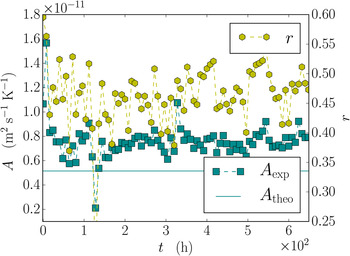
To assess the temporal evolution of the growth law parameter A, a linear fit and the sample Pearson correlation coefficient r is evaluated for the entire time-lapse experiment and shown in Figure 11. The results show that the measured values of A are close to the theoretical value.

In the next step we analyzed the statistical significance of the presence of a curvature dependent term in the data. To this end we first fitted the data to the coarsening growth law Eqn (12). The results of the estimates B exp are shown in Figure 12. The correlation coefficients found here are in the same order as for the isothermal experiment (Figs 7 and 8).

It is thus reasonable to also assess the linear combination of Eqns (9) and (12):
 $${v_n} = A{\bf\nabla} T \cdot {\bf n} + \displaystyle{B \over \lambda} \left( {\overline H - H} \right). $$
The values for A and B are similar to those obtained before (not shown). However the correlation coefficient changes, depending on the growth law that is used. We first assessed r
A by fitting A to Eqn (9). Secondly we calculated r
B where B is fitted to Eqn (12). Finally r
A,B is computed where A and B are simultaneously fitted in the combined growth law, Eqn (27). The time-evolution of these coefficients is plotted in Figure 13. The data show that ${\overline r _{_{\rm B}}} \approx 0.30$
,
${\overline r _{_{\rm B}}} \approx 0.30$
, ${\overline r _{_{\rm A}}} \approx 0.46$
and
${\overline r _{_{\rm A}}} \approx 0.46$
and ${\overline r _{_{{\rm A,B}}}} \approx 0.57$
.
${\overline r _{_{{\rm A,B}}}} \approx 0.57$
.

4.2.5. Sensitivity analysis
Finally, we assess the impact of the limit parameter ε introduced in Section 3.3. To this end we have analyzed the dependence of the growth law coefficient A on ε for one sample at t = 0. The results are shown in Figure 14. Our choice of ε = 1.25 used for the analysis of all the samples then corresponds to the minimal sensitivity of this parameter. The dependence on ε will be further detailed in the discussion.

5. DISCUSSION
5.1. Curvature driven metamorphism
For isothermal metamorphism, we compared the interface velocities data obtained by the proposed interface tracking method, using two available models: diffusion limited growth, Eqn (12) and kinetics limited growth, Eqn (14). For the diffusion limited model (Fig. 6, top) the data revealed a large scatter around the origin and the scatter plots are difficult to interpret visually due to the symmetric appearance of the data. However, we observed a weak but consistent correlation (Fig. 7) when fitting the data to the diffusion limited growth law, Eqn (12). The fitted values, B exp are higher than the theoretical value B theo. If Eqn (12) was strictly valid, a possible explanation of the high B exp values would be an underestimation of the mean curvatures. We recall that our curvature estimates rely on the smoothing parameter, which had to be chosen subjectively, and smoothing predominantly reduces always high curvature regions. Another explanation could be the presence of surface diffusion, which is neglected in Eqn (12). If surface diffusion played a role it would increase the value for the estimated B exp, since both processes simultaneously contribute to the reduction of mean curvature. As suggested by Tomita (Reference Tomita2000), surface diffusion should manifest itself as a higher order correction to Eqn (12) according to
 $${v_n} = \displaystyle{B \over \lambda} (1 - {\lambda ^2}{\bf\nabla} _{\rm S}^2 )[\overline H - H], $$
with ${\bf\nabla} _{\rm S}^2 $
the surface Laplacian. It will, in principal, be possible to also evaluate the growth law Eqn (28) and discern effects of surface diffusion and bulk vapor diffusion. However this would require higher quality experimental data. The available dataset for new snow with a voxel size 10 µm is presently at the limit of resolution, where curvatures can be estimated reliably, as can be seen from Figure 5. The algorithms used by Flin and others (Reference Flin2005) and Brzoska and others (Reference Brzoska, Flin, Ogawa and Kuhs2007) use a different smoothing procedure and might give an improved curvature estimation for fresh snow, which would enable the analysis of surface diffusion dependent growth laws. Previous results (Löwe and others, Reference Löwe, Spiegel and Schneebeli2011) in fact suggest that surface diffusion does play a role at lower temperatures. This is indicated by the exponent governing the power law decrease of the specific surface area, which is closer to 1/4, indicating surface diffusion, than to 1/3 indicating bulk diffusion.
${\bf\nabla} _{\rm S}^2 $
the surface Laplacian. It will, in principal, be possible to also evaluate the growth law Eqn (28) and discern effects of surface diffusion and bulk vapor diffusion. However this would require higher quality experimental data. The available dataset for new snow with a voxel size 10 µm is presently at the limit of resolution, where curvatures can be estimated reliably, as can be seen from Figure 5. The algorithms used by Flin and others (Reference Flin2005) and Brzoska and others (Reference Brzoska, Flin, Ogawa and Kuhs2007) use a different smoothing procedure and might give an improved curvature estimation for fresh snow, which would enable the analysis of surface diffusion dependent growth laws. Previous results (Löwe and others, Reference Löwe, Spiegel and Schneebeli2011) in fact suggest that surface diffusion does play a role at lower temperatures. This is indicated by the exponent governing the power law decrease of the specific surface area, which is closer to 1/4, indicating surface diffusion, than to 1/3 indicating bulk diffusion.
If the data are fitted to the kinetics limited growth law, Eqn (14) instead (Fig. 6, bottom), the correlation coefficient slightly increases (Fig. 8). Within the limited accuracy of the data, we conclude that kinetics cannot be completely ignored. This is consistent with the dominant snow type (PPpl) of the sample, which contains many plate-like structures, where kinetics should play a crucial role on the basal orientations of the plates (Libbrecht, Reference Libbrecht2005). The same kinetics limited growth law (Eqn (14)) was already suggested by Flin and others (Reference Flin, Brzoska, Lesaffre, Coléou and Pieritz2003) to model isothermal metamorphism.
Our experimental setup bears another uncertainty in the order of one voxel in x-, y- and z-direction (Section 3.5), which stems from the uncertainty in absolute position. Here the experimental setup developed by Calonne and others (Reference Calonne2015) might improve on that, since the sample is left at exactly the same position during the time-series. Another difficulty encountered here for the isothermal dataset is the necessity of correcting for settling effects. We outlined that the motion of an interface by crystal growth and the motion of the interface by gravitational settling can a priori not be discerned. On one hand, large specific surface areas are required to ensure a good signal-to-noise ratio for metamorphism. On the other hand, large specific surface areas increase the effect of settling (Schleef and others, Reference Schleef, Löwe and Schneebeli2014). In new snow, the crystals experience significant displacements, which are larger than the size of the particles. It is difficult to compensate for these effects automatically. In addition the settling is not uniform, as assumed in Eqn (26). In the future, an ideal isothermal experiment would comprise artificially compacted, slightly sintered new snow in order to minimize settling effects with reasonably high curvature for significant growth effects.
5.2. Temperature gradient driven metamorphism
As a reference model, the obtained data were compared with the generalization of the classical picture from Shreve (Reference Shreve1967) for the migration of vapor bubbles in ice. Despite its simplicity, the model is still used as a reference to analyze experiments for the migration of vapor bubbles in ice (Dadic and others, Reference Dadic, Light and Warren2010). In the Shreve picture, the local interface velocities are mainly determined by the local temperature gradient in the pore space. For a single sphere, the simplicity of the geometry allows us to compute the temperature gradient in the pore space analytically. This can be generalized to complex microstructures, if the temperature gradients are computed numerically. Our results revealed that, on average, the Shreve picture holds reasonably well for the entire snow structure. Compared with the isothermal case, we found less scatter in the histograms (Fig. 10) and estimated values A exp, which are in the same order of magnitude as the theoretical value for the entire time series (Fig. 11). The estimate A exp is fairly constant over time, implying that on average, the relation between the interface velocities and the temperature gradient constitute an important physical contribution to the growth under temperature gradients. However, the fact that facets and depth hoar emerge during metamorphism clearly indicates that the purely diffusion limited picture, Eqn (9) cannot be strictly valid.
In addition, we analyzed an empirical, linear superposition of the curvature and gradient driven processes, cf. Eqn (27). Again, the analysis shows a low correlation implying a slight influence of the curvature term, but less pronounced than the temperature gradient contribution (Fig. 13). Similar to the isothermal analysis, the estimated values for B exp are higher than their theoretical value. The same explanations given for the isothermal case are applicable here. A comparison with the isothermal case is however difficult due to the differences in their apparent kinetic regime, temperature, voxel resolution and initial snow type.
The analysis of the temperature gradient growth law has revealed another uncertainty, namely the numerical solution of the temperature field. A subtle source of error originates from the numerical solution on voxel-based images for the proposed method of estimating the temperature gradients in the pore space (Section 3.3). The temperature gradient must be computed in the limit of approaching the interface from the vapor space in Eqn (9). This sampling must be close enough to the interface to represent the vapor-space near the interface, but not too close since the sampling will be in the ice phase for a fraction of the points, resulting in a lower value for the average temperature gradient, and higher values for A. If the sampling were too far away from the interface, temperature gradients would decrease, resulting in a higher value for A, as observed in the sensitivity analysis (Fig. 14). Accordingly we have chosen the spatial distance ε from the interface to be in the order of one voxel, more precisely ε = 1.25 m which corresponds to the minimum of the sensitivity. The choice and sensitivity of the results on ε are closely related to the accuracy of the numerical solution of the temperature distribution at that point. The numerical solution (Pinzer and others, Reference Pinzer, Schneebeli and Kaempfer2012) implements the two-phase material by a space-dependent thermal conductivity, which changes discontinuously from the ice conductivity κ i to the air conductivity κ a at the interface. Theoretically, the interface condition Eqn (5) should be recovered. An a posteriori analysis was made of the interface condition by computing the ratio
 $$\displaystyle{{{{\left. {{\bf\nabla} T \cdot {\bf n}} \right \vert} _ -}} \over {{{\left. {{\bf\nabla} T \cdot {\bf n}} \right \vert} _ +}}} = {\kappa _{\rm a}}/{\kappa _{\rm i}}. $$
Theoretically the ratio should assume a value of ≈ 0.01. From the simulations, an average ratio close to 0.125 was found, with significant scatter. This is a clear indication of limited accuracy close to the interface on a voxel mesh. This implies uncertainties of the estimated A up to a factor of 12.5. The origin of this uncertainty is the voxel based finite element solutions, which are commonly used (Pinzer and others, Reference Pinzer, Schneebeli and Kaempfer2012; Löwe and others, Reference Löwe, Riche and Schneebeli2013; Calonne and others, Reference Calonne, Flin, Geindreau, Lesaffre and Rolland du Roscoat2014a) and which are also applied here. Apparently, the present case of discontinuous coefficients clearly requires more sophisticated methods (Soghrati and others, Reference Soghrati, Aragón, Armando Duarte and Geubelle2012) to ensure reasonable accuracy of the solution at the interface.
A crucial aspect of the temperature gradient analysis is the temporal resolution of the time-lapse experiment. The analysis has shown that interface tracking is feasible, but limited by the resolution of μCT time series. The time difference of 8 hours has turned out to be too high to avoid the loss of interface correlations between two consecutive images. The optimal temporal resolution depends on typical sizes of the structure, which could for example be assessed by the dimensionless quantity, Eqn (24). The interface dynamics of small features naturally requires a higher temporal and spatial resolution. Consecutive interfaces also become decorrelated during structural re-arrangements triggered by growth under gravity and this was occasionally observed. Such a mechanism of ‘dropping grains’ has been employed by Vetter and others (Reference Vetter2010) for isothermal metamorphism. These events contribute to the scatter in the velocity, since dropping structures cannot be registered anymore by the interface tracking.
Overall the temperature gradient analysis is less affected by the influence of settling due to the higher initial density and the faster growth during temperature gradient metamorphism. But in contrast to the isothermal case, where vapor transport and growth are isotropic, here the main growth direction (temperature gradient) and the main settling direction (gravity) are the same. An ideal experimental setup would realize a temperature gradient perpendicular to gravity, or at least reverse the direction of the temperature gradient to better discern these effects.
6. CONCLUSIONS
A first attempt has been made to measure the local interface dynamics of the ice/air interface in snow from μCT time-lapse experiments and to interpret the data in terms of non-equilibrium vapor processes at the pore level. We have developed an interface tracking method for time-lapse experiments and compared the measured normal velocities with the simplest, isotropic diffusion limited and kinetics limited growth models that are applicable to bicontinuous structures. While the growth rates predicted by these models are in the same order of magnitude as the experimental data, a final conclusion about this coincidence is not yet possible. This is due to the large scatter, which was discussed and related to experimental, theoretical and methodological limitations. Given the possible improvements suggested from the analysis, it seems promising to further advance the method, and validate growth laws as required for the upscaling in macroscopic snow modeling.
ACKNOWLEDGEMENTS
We thank Michael Lehning and Martin Schneebeli for stimulating discussions and gratefully acknowledge careful suggestions from Frederic Flin during the review process. The work was funded by the Swiss National Science Foundation (SNSF), Grant No. 200021_143839.


 Open access