





1. Introduction
The solar wind is a magnetised plasma that rapidly becomes supersonic as it flows away from the Sun and into the heliosphere. Some of the earliest evidence for the existence of the solar wind came from Biermann (Reference Biermann1952), who inferred a solar-wind velocity $U\sim 500{-}1500\,\mathrm{km}\,\mathrm{s}^{-1}$
from observations of comet tails. These observations led to the discovery that a hot solar corona could accelerate the solar wind to supersonic speeds via a thermal pressure gradient (Parker Reference Parker1958). Since the first direct satellite measurements of the solar wind (Gringauz et al. Reference Gringauz, Bezrokikh, Ozerov and Rybchinskii1960), it has been characterised into two distinct phases based on velocity: fast
$U\sim 500{-}1500\,\mathrm{km}\,\mathrm{s}^{-1}$
from observations of comet tails. These observations led to the discovery that a hot solar corona could accelerate the solar wind to supersonic speeds via a thermal pressure gradient (Parker Reference Parker1958). Since the first direct satellite measurements of the solar wind (Gringauz et al. Reference Gringauz, Bezrokikh, Ozerov and Rybchinskii1960), it has been characterised into two distinct phases based on velocity: fast $(U\gtrsim 700\,\mathrm{km}\,\mathrm{s}^{-1})$
and slow
$(U\gtrsim 700\,\mathrm{km}\,\mathrm{s}^{-1})$
and slow $(U\lesssim 400\,\mathrm{km}\,\mathrm{s}^{-1})$
; though, there is growing evidence that Alfvénicity, or correlation between fluctuations in the plasma velocity and magnetic field, and the composition of minor ions reveal at least two types of slow solar wind (see D’Amicis et al. (Reference D’Amicis, Perrone, Bruno and Velli2021), and references therein). Recent work has suggested that, past the Alfvén critical point (or, more realistically, Alfvén surface; see Badman et al. Reference Badman2025) – where the solar wind becomes super-Alfvénic – the acceleration of the slow solar wind is best explained by gradients in the electron-enthalpy and heat fluxes and that of the fast solar wind is explained by gradients in the flux of energy carried by Alfvén waves that are travelling away from the Sun (Halekas et al. Reference Halekas2023; Rivera et al. Reference Rivera2025).
$(U\lesssim 400\,\mathrm{km}\,\mathrm{s}^{-1})$
; though, there is growing evidence that Alfvénicity, or correlation between fluctuations in the plasma velocity and magnetic field, and the composition of minor ions reveal at least two types of slow solar wind (see D’Amicis et al. (Reference D’Amicis, Perrone, Bruno and Velli2021), and references therein). Recent work has suggested that, past the Alfvén critical point (or, more realistically, Alfvén surface; see Badman et al. Reference Badman2025) – where the solar wind becomes super-Alfvénic – the acceleration of the slow solar wind is best explained by gradients in the electron-enthalpy and heat fluxes and that of the fast solar wind is explained by gradients in the flux of energy carried by Alfvén waves that are travelling away from the Sun (Halekas et al. Reference Halekas2023; Rivera et al. Reference Rivera2025).
The vast majority of the Alfvén-wave flux is at scales that are much too large to directly heat the solar wind. Most likely, the transfer of wave energy from large to small scales is facilitated by a nonlinear cascade (Coleman Reference Coleman1968; Velli, Grappin & Mangeney Reference Velli, Grappin and Mangeney1989; Matthaeus et al. Reference Matthaeus, Zank, Oughton, Mullan and Dmitruk1999; Cranmer & van Ballegooijen Reference Cranmer and van Ballegooijen2005). The most vigorous Alfvén-wave cascades result from collisions between counter-propagating wave packets. Outward-propagating Alfvén waves undergo a small amount of linear (non-WKB) reflection due to gradients in the background magnetic field and density (Heinemann & Olbert Reference Heinemann and Olbert1980). The presence of reflected waves is sufficient to initiate a nonlinear cascade that transports energy to small scales (Dmitruk et al. Reference Dmitruk, Matthaeus, Milano, Oughton, Zank and Mullan2002), where it can be dissipated (Cranmer & van Ballegooijen Reference Cranmer and van Ballegooijen2003). Indeed, a number of solar-wind models (Cranmer et al. Reference Cranmer, van, Adriaan and Edgar2007; Verdini et al. Reference Verdini, Velli, Matthaeus, Oughton and Dmitruk2010) have demonstrated that reflection-driven turbulence is sufficient to heat and accelerate the fast solar wind to observed velocities.
Despite the growing consensus that the cascade of anti-sunward Alfvén waves can power the fast solar wind, it is still not entirely clear what mechanisms are responsible for converting the energy in the turbulent fluctuations into particle heat and momentum. A complicating factor in discerning the relevant mechanisms is the fact that the solar wind is weakly collisional, with the mean free path for Coulomb collisions reaching the largest characteristic scales of the solar wind (Verscharen, Klein & Maruca Reference Verscharen, Klein and Maruca2019). One clue towards resolving this mystery is the observation that proton heating dominates electron heating by $4:1$
in the fast solar wind (Bandyopadhyay et al. Reference Bandyopadhyay2023). When the energy in the background magnetic field dominates the thermal energy – as it does in the inner heliosphere – protons are generally understood to be collisionlessly heated through one of two observationally distinct mechanisms: resonant cyclotron heating by ion cyclotron waves (ICWs) (Kennel & Engelmann Reference Kennel and Engelmann1966; Hollweg & Isenberg Reference Hollweg and Isenberg2002; Isenberg & Vasquez Reference Isenberg and Vasquez2011), or via a non-resonant process called stochastic heating (McChesney, Stern & Bellan Reference McChesney, Stern and Bellan1987; Chaston et al. Reference Chaston, Bonnell, Carlson, McFadden, Ergun, Strangeway and Lund2004; Chandran et al. Reference Chandran, Li, Rogers, Quataert and Germaschewski2010a
; Bourouaine & Chandran Reference Bourouaine and Chandran2013).Footnote
1
Recent work analysing data from Parker Solar Probe (PSP) has provided observational evidence that ICW heating is an important mechanism for proton heating in the fast, super-Alfvénic solar wind (Bowen et al. Reference Bowen2022; Shankarappa et al. Reference Shankarappa, Klein, Martinović and Bowen2024).
$4:1$
in the fast solar wind (Bandyopadhyay et al. Reference Bandyopadhyay2023). When the energy in the background magnetic field dominates the thermal energy – as it does in the inner heliosphere – protons are generally understood to be collisionlessly heated through one of two observationally distinct mechanisms: resonant cyclotron heating by ion cyclotron waves (ICWs) (Kennel & Engelmann Reference Kennel and Engelmann1966; Hollweg & Isenberg Reference Hollweg and Isenberg2002; Isenberg & Vasquez Reference Isenberg and Vasquez2011), or via a non-resonant process called stochastic heating (McChesney, Stern & Bellan Reference McChesney, Stern and Bellan1987; Chaston et al. Reference Chaston, Bonnell, Carlson, McFadden, Ergun, Strangeway and Lund2004; Chandran et al. Reference Chandran, Li, Rogers, Quataert and Germaschewski2010a
; Bourouaine & Chandran Reference Bourouaine and Chandran2013).Footnote
1
Recent work analysing data from Parker Solar Probe (PSP) has provided observational evidence that ICW heating is an important mechanism for proton heating in the fast, super-Alfvénic solar wind (Bowen et al. Reference Bowen2022; Shankarappa et al. Reference Shankarappa, Klein, Martinović and Bowen2024).
Curiously, much of the ICW heating observed in the fast, super-Alfvénic solar wind is found to be facilitated by parallel ICWs (PICWs), which are circularly polarised and propagate nearly parallel to the background magnetic field (Liu et al. Reference Liu, Zhao, Wang, Dong, Kasper, Bale, Shi and Wu2023). Such PICWs are pervasive in the inner heliosphere, appearing continuously for large segments of nearly every PSP encounter (Shankarappa et al. Reference Shankarappa, Klein, Martinović, Bowen, Larson, Livi, Rahmati, Whittlesey and Stevens2025). They are also observed in a narrow band of wavenumbers parallel to the background magnetic field, $k_\parallel$
, centred around
$k_\parallel$
, centred around $k_\parallel d_{\mathrm{p}}\sim 1$
(Bowen et al. Reference Bowen2024b
). Here,
$k_\parallel d_{\mathrm{p}}\sim 1$
(Bowen et al. Reference Bowen2024b
). Here, $d_{\mathrm{p}}=v_{\mathrm{A}}/\varOmega _{\mathrm{p}}$
is the proton inertial length,
$d_{\mathrm{p}}=v_{\mathrm{A}}/\varOmega _{\mathrm{p}}$
is the proton inertial length, $v_{\mathrm{A}}=B/\sqrt {4\pi nm_{\mathrm{p}}}$
is the Alfvén velocity,
$v_{\mathrm{A}}=B/\sqrt {4\pi nm_{\mathrm{p}}}$
is the Alfvén velocity, $\varOmega _{\mathrm{p}}=q_{\mathrm{p}}B/m_{\mathrm{p}}c$
is the proton gyrofrequency,
$\varOmega _{\mathrm{p}}=q_{\mathrm{p}}B/m_{\mathrm{p}}c$
is the proton gyrofrequency, $B$
is the magnitude of the background magnetic field,
$B$
is the magnitude of the background magnetic field, $c$
is the speed of light and
$c$
is the speed of light and $n$
,
$n$
, $q_{\mathrm{p}}$
and
$q_{\mathrm{p}}$
and $m_{\mathrm{p}}$
are the proton number density, charge and mass, respectively. Because PICWs are so separated in wave vector from the turbulent cascade of Alfvén waves (that become oblique ICWs when
$m_{\mathrm{p}}$
are the proton number density, charge and mass, respectively. Because PICWs are so separated in wave vector from the turbulent cascade of Alfvén waves (that become oblique ICWs when $k_\parallel d_{\rm p}\sim 1$
), it is unlikely they can be generated from the cascade by nonlinear wave–wave interactions (Zakharov, L’Vov & Falkovich Reference Zakharov, L’Vov and Falkovich1992; Alexakis et al. Reference Alexakis, Bigot, Politano and Galtier2007). A number of authors have proposed that PICWs might originate via quasi-linear focusing (Chandran et al. Reference Chandran, Pongkitiwanichakul, Isenberg, Lee, Markovskii, Hollweg and Vasquez2010b
; Isenberg & Vasquez Reference Isenberg and Vasquez2011). In quasi-linear focusing, heating by a turbulent cascade of oblique ICWs causes the proton velocity distribution to become so anisotropic that PICWs become unstable and grow, leading to a transfer of energy from oblique ICWs to PICWs through protons that are co-resonant with both waves. Quasi-linear focusing is also the most likely explanation for the emission of PICWs in hybrid-particle-in-cell simulations of imbalanced Alfvénic turbulence (Squire et al. Reference Squire, Meyrand, Kunz, Arzamasskiy, Schekochihin and Quataert2022; Zhang et al. Reference Zhang, Kunz, Squire and Klein2025).
$k_\parallel d_{\rm p}\sim 1$
), it is unlikely they can be generated from the cascade by nonlinear wave–wave interactions (Zakharov, L’Vov & Falkovich Reference Zakharov, L’Vov and Falkovich1992; Alexakis et al. Reference Alexakis, Bigot, Politano and Galtier2007). A number of authors have proposed that PICWs might originate via quasi-linear focusing (Chandran et al. Reference Chandran, Pongkitiwanichakul, Isenberg, Lee, Markovskii, Hollweg and Vasquez2010b
; Isenberg & Vasquez Reference Isenberg and Vasquez2011). In quasi-linear focusing, heating by a turbulent cascade of oblique ICWs causes the proton velocity distribution to become so anisotropic that PICWs become unstable and grow, leading to a transfer of energy from oblique ICWs to PICWs through protons that are co-resonant with both waves. Quasi-linear focusing is also the most likely explanation for the emission of PICWs in hybrid-particle-in-cell simulations of imbalanced Alfvénic turbulence (Squire et al. Reference Squire, Meyrand, Kunz, Arzamasskiy, Schekochihin and Quataert2022; Zhang et al. Reference Zhang, Kunz, Squire and Klein2025).
An outstanding issue with quasi-linear focusing explaining observations of PICWs is that the waves are often observed to heat the solar wind (Bowen et al. Reference Bowen2022, Reference Bowen2024b ). Quasi-linear focusing is a process of PICW emission, not absorption, in which PICWs cool, rather than heat, the solar wind. The resolution of this issue is the primary focus of this work. We start with § 2, where we introduce the necessary background and machinery to understand quasi-linear focusing. That section includes the dispersion relations we use for both oblique ICWs and PICWs (§ 2.1), an introduction to the linear stability of ICWs in § 2.2 and an explanation of how the oblique ICW cascade can drive PICWs unstable in § 2.3. With the necessary background established, we present the main result of this work, cyclotron breaking, in § 3. We begin § 3 with a quick primer on the turbulent transition range (§ 3.1), followed by a discussion on how the transition range affects quasi-linear focusing by limiting the band of wavenumbers in which oblique ICW heating is strong and therefore PICWs are unstable (§ 3.2). We then show that, as the resulting unstable PICWs propagate away from the Sun, they evolve so as to resonate with slower and slower protons. Eventually, PICWs will resonate with protons that are too slow to be resonantly heated by the turbulent cascade, at which point the PICWs will damp and heat the solar wind (§ 3.3).
2. Parallel ICWs driven unstable by the turbulent cascade
In this section, we discuss how PICWs are driven unstable by an imbalanced turbulent cascade of oblique ICWs. It should be stated that the discussion here applies strictly for a homogeneous medium. However, in an inhomogeneous medium, corrections to the homogeneous dispersion relation will be $O(1/k_\parallel L)$
, where
$O(1/k_\parallel L)$
, where $L$
is a characteristic length scale
$L$
is a characteristic length scale $|{\mathrm{d}}\ln B/{\mathrm{d}} r|^{-1}$
or
$|{\mathrm{d}}\ln B/{\mathrm{d}} r|^{-1}$
or $|{\mathrm{d}} \ln n/{\mathrm{d}} r|^{-1}$
. Taking
$|{\mathrm{d}} \ln n/{\mathrm{d}} r|^{-1}$
. Taking $k_\parallel d_{\mathrm{p}}\sim 1$
, these corrections are at most
$k_\parallel d_{\mathrm{p}}\sim 1$
, these corrections are at most $O(10^{-6})$
in the inner heliosphere and can therefore be safely ignored. In addition, we assume that the turbulent spectrum driving the PICWs consists of oblique ICWs (as defined in § 2.1) and that it is imbalanced, i.e. that there is much more energy in waves propagating anti-sunward than sunward in the plasma rest frame. A fully self-consistent, hot-plasma treatment would make the following analysis analytically intractable, so we approximate the real part of the wave frequencies,
$O(10^{-6})$
in the inner heliosphere and can therefore be safely ignored. In addition, we assume that the turbulent spectrum driving the PICWs consists of oblique ICWs (as defined in § 2.1) and that it is imbalanced, i.e. that there is much more energy in waves propagating anti-sunward than sunward in the plasma rest frame. A fully self-consistent, hot-plasma treatment would make the following analysis analytically intractable, so we approximate the real part of the wave frequencies, $\omega _{k{\mathrm{r}}}$
, using the cold-plasma dispersion relation and then use the quasi-linear analysis of Kennel & Wong (Reference Kennel and Wong1967) to evaluate the sign of the imaginary part of the wave frequency,
$\omega _{k{\mathrm{r}}}$
, using the cold-plasma dispersion relation and then use the quasi-linear analysis of Kennel & Wong (Reference Kennel and Wong1967) to evaluate the sign of the imaginary part of the wave frequency, $\gamma$
. For a discussion of how the simple depiction of quasi-linear focusing depicted here is adapted to the solar wind, see § 3.
$\gamma$
. For a discussion of how the simple depiction of quasi-linear focusing depicted here is adapted to the solar wind, see § 3.
2.1. Cold-plasma dispersion relations for ion cyclotron waves
The real frequency $\omega _{k{\mathrm{r}}}$
of an ICW with wavenumbers
$\omega _{k{\mathrm{r}}}$
of an ICW with wavenumbers $k_\parallel$
and
$k_\parallel$
and $k_\perp$
, parallel and perpendicular to the background magnetic field, respectively, can be approximated by the cold-plasma dispersion relation (equation (21) in chapter 2 of Stix (Reference Stix1992)):
$k_\perp$
, parallel and perpendicular to the background magnetic field, respectively, can be approximated by the cold-plasma dispersion relation (equation (21) in chapter 2 of Stix (Reference Stix1992)):
 \begin{align} \omega _{k{\mathrm{r}}}= \varOmega _{\mathrm{p}}\sqrt { \dfrac {1}{2}\big(b-\sqrt {b^2-4c}\big)}, \end{align}
where
 \begin{align} b&=(k d_{\mathrm{p}})^2 + (k_\parallel d_{\mathrm{p}})^2 + c,\\[-8pt]\nonumber \end{align}
 \begin{align} c &= k^2k_\parallel ^2d_{\mathrm{p}}^4. \end{align}
Here, $k=(k_\parallel ^2+k_\perp ^2)^{1/2}$
is the magnitude of the wavenumber. If we now set
$k=(k_\parallel ^2+k_\perp ^2)^{1/2}$
is the magnitude of the wavenumber. If we now set $k_\perp =0$
, we obtain the PICW dispersion relation (Hollweg & Isenberg Reference Hollweg and Isenberg2002):
$k_\perp =0$
, we obtain the PICW dispersion relation (Hollweg & Isenberg Reference Hollweg and Isenberg2002):
 \begin{align} \omega _{k_\parallel {\mathrm{r}},{\rm P}} =\dfrac {\varOmega _{\mathrm{p}}(k_\parallel d_{\mathrm{p}})^2}{2}\Big[\sqrt {1+4(k_\parallel d_{\mathrm{p}})^{-2}}-1\Big]. \end{align}
2.2. Ion cyclotron wave stability
The linear stability of a plasma to a given wave mode is entirely due to the preferred direction of energy exchange between the wave mode and particle population, as mediated by resonant wave–particle interactions. Waves and particles, here cyclotron waves and protons, interact resonantly when $\omega _{k{\mathrm{r}}}$
, as measured in a frame moving along the background magnetic field at the parallel velocity of the proton
$\omega _{k{\mathrm{r}}}$
, as measured in a frame moving along the background magnetic field at the parallel velocity of the proton $v_\parallel$
, is an integer (
$v_\parallel$
, is an integer ( $n$
) multiple of the proton cyclotron frequency
$n$
) multiple of the proton cyclotron frequency $\varOmega _{\mathrm{p}}$
(Stix Reference Stix1992), i.e.
$\varOmega _{\mathrm{p}}$
(Stix Reference Stix1992), i.e.
 \begin{align} \omega _{k{\mathrm{r}}}-k_\parallel v_\parallel =n\varOmega _{\mathrm{p}}. \end{align}
Here, $v_\parallel$
is measured in the frame travelling at the solar-wind velocity
$v_\parallel$
is measured in the frame travelling at the solar-wind velocity $U$
. One can solve (2.3) either for
$U$
. One can solve (2.3) either for $k_{\parallel \mathrm{res}}=k_{\parallel \mathrm{res}}(v_\parallel ,k_\perp ,n)$
, the
$k_{\parallel \mathrm{res}}=k_{\parallel \mathrm{res}}(v_\parallel ,k_\perp ,n)$
, the $k_\parallel$
of a wave with given
$k_\parallel$
of a wave with given $k_\perp$
whose
$k_\perp$
whose $n{\mathrm{th}}$
cyclotron harmonic is resonant with a particle travelling at
$n{\mathrm{th}}$
cyclotron harmonic is resonant with a particle travelling at $v_\parallel$
, or for
$v_\parallel$
, or for
 \begin{align} v_{\parallel \mathrm{res}}(k_\parallel ,k_\perp ,n) = \dfrac {\omega _{k{\mathrm{r}}}-n\varOmega _{\mathrm{p}}}{k_\parallel }, \end{align}
the velocity of a particle that is resonant with the $n{\mathrm{th}}$
cyclotron harmonic of a wave with a given
$n{\mathrm{th}}$
cyclotron harmonic of a wave with a given $k_\parallel$
and
$k_\parallel$
and $k_\perp$
.
$k_\perp$
.
For $n=0$
,
$n=0$
, $v_{\parallel \mathrm{res}} = \omega _{k{\mathrm{r}}}/k_\parallel$
, i.e. the parallel resonant velocity for a given wave is its phase speed. The
$v_{\parallel \mathrm{res}} = \omega _{k{\mathrm{r}}}/k_\parallel$
, i.e. the parallel resonant velocity for a given wave is its phase speed. The $n=0$
resonance is often referred to as the Landau resonance. Landau-resonant wave–particle interactions can be mediated by the component of the electric field parallel to the magnetic field, as is the case with Landau damping, or by the electric field components perpendicular to the magnetic field, as is the case with transit-time damping (Stix Reference Stix1992). Qualitatively, if the derivative of the proton velocity distribution function,
$n=0$
resonance is often referred to as the Landau resonance. Landau-resonant wave–particle interactions can be mediated by the component of the electric field parallel to the magnetic field, as is the case with Landau damping, or by the electric field components perpendicular to the magnetic field, as is the case with transit-time damping (Stix Reference Stix1992). Qualitatively, if the derivative of the proton velocity distribution function, $f_{\mathrm{p}}$
, with respect to
$f_{\mathrm{p}}$
, with respect to $v_\parallel$
has the same sign as the wave phase velocity,
$v_\parallel$
has the same sign as the wave phase velocity, $\omega _{k{\mathrm{r}}}/k_\parallel$
, in the immediate vicinity of the resonant velocity
$\omega _{k{\mathrm{r}}}/k_\parallel$
, in the immediate vicinity of the resonant velocity $v_\parallel =\omega _{k{\mathrm{r}}}/k_\parallel$
, more protons will give energy to the wave than take away from it. The net effect will be wave growth – instability. Conversely, wave energy will be absorbed (damped) if the opposite is true.
$v_\parallel =\omega _{k{\mathrm{r}}}/k_\parallel$
, more protons will give energy to the wave than take away from it. The net effect will be wave growth – instability. Conversely, wave energy will be absorbed (damped) if the opposite is true.
When $n\ne 0$
, the wave–particle interactions are said to be cyclotron resonant. Consider a single plane wave. In the ‘wave frame’, which moves at the wave phase velocity along the background magnetic field
$n\ne 0$
, the wave–particle interactions are said to be cyclotron resonant. Consider a single plane wave. In the ‘wave frame’, which moves at the wave phase velocity along the background magnetic field $\hat{\boldsymbol{b}} \omega /k_\parallel$
(here
$\hat{\boldsymbol{b}} \omega /k_\parallel$
(here $\hat {\boldsymbol{b}}=\boldsymbol{B}/B$
is the unit vector along the magnetic field), the partial time derivative of the wave fields vanishes, and the total particle energy
$\hat {\boldsymbol{b}}=\boldsymbol{B}/B$
is the unit vector along the magnetic field), the partial time derivative of the wave fields vanishes, and the total particle energy $H = ({1}/{2}) mv^2 + q_{\mathrm{p}} \varPhi$
is constant, where
$H = ({1}/{2}) mv^2 + q_{\mathrm{p}} \varPhi$
is constant, where $\varPhi$
is the electrostatic potential. For small-amplitude waves,
$\varPhi$
is the electrostatic potential. For small-amplitude waves, $\varPhi$
is a constant plus a small sinusoidal oscillation. Therefore, the particle kinetic energy
$\varPhi$
is a constant plus a small sinusoidal oscillation. Therefore, the particle kinetic energy $({1}/{2}) m_{\mathrm{p}} v^2$
undergoes only small oscillations, cannot change secularly and is effectively conserved. Cyclotron-resonant wave–particle interactions can, however, cause particles to diffuse in the
$({1}/{2}) m_{\mathrm{p}} v^2$
undergoes only small oscillations, cannot change secularly and is effectively conserved. Cyclotron-resonant wave–particle interactions can, however, cause particles to diffuse in the $v_\parallel {-} v_\perp$
plane along contours of constant energy in the wave frame, which are defined by the equation (Kennel & Engelmann Reference Kennel and Engelmann1966)
$v_\parallel {-} v_\perp$
plane along contours of constant energy in the wave frame, which are defined by the equation (Kennel & Engelmann Reference Kennel and Engelmann1966)
 \begin{align} \bigg(v_\parallel -\dfrac {\omega _{k{\mathrm{r}}}}{k_\parallel }\Big|_{k_{\parallel \mathrm{res}}} \bigg)^2 + v_\perp ^2 = {\mathrm{const}}. \end{align}
The solutions to (2.5) are called quasi-linear contours. The intuition behind the stability of cyclotron-resonant waves (like ion cyclotron and whistler waves) is much the same as waves mediated by the Landau resonance. However, the relevant velocity-space derivative of $f_{\mathrm{p}}$
is given by the differential operator (Kennel & Wong Reference Kennel and Wong1967)
$f_{\mathrm{p}}$
is given by the differential operator (Kennel & Wong Reference Kennel and Wong1967)
 \begin{align} G=\left (\left .\dfrac {\omega _{k{\mathrm{r}}}}{k_\parallel }\right . -v_\parallel \right )\frac {\partial }{\partial v_\perp }+v_\perp \frac {\partial }{\partial v_\parallel }, \end{align}
which calculates the derivative of its operand along the quasi-linear contours (2.5). To determine the stability of a wave mode, one must consider the net effect of all the resonant particles. Indeed, this consideration is taken into account in the full calculation of the linear growth rate in Kennel & Wong (Reference Kennel and Wong1967). For PICWs, one can show that the growth rate $\gamma _{\mathrm{P}}(k_\parallel )$
is positive when
$\gamma _{\mathrm{P}}(k_\parallel )$
is positive when
 \begin{align} \gamma _{\mathrm{P}}(k_\parallel )\propto {\mathrm{sign}}\left (\left .\dfrac {\omega _{k_\parallel {\mathrm{r}},P}}{k_\parallel }\right . \right )\int _0^\infty {\mathrm{d}}v_\perp \,v_\perp ^2\left .\left [G_{\mathrm{P}}f_{\mathrm{p}}(v_\parallel ,v_\perp )\right ]\right |_{v_{\parallel {\mathrm{P}}}} \gt 0. \end{align}
Here, $G_{\mathrm{P}}$
is the differential operator
$G_{\mathrm{P}}$
is the differential operator $G$
of (2.6) evaluated for
$G$
of (2.6) evaluated for $\omega _{k{\mathrm{r}}}=\omega _{k_\parallel {\mathrm{r}},{\rm P}}$
and
$\omega _{k{\mathrm{r}}}=\omega _{k_\parallel {\mathrm{r}},{\rm P}}$
and $v_{\parallel {\mathrm{P}}}=v_{\parallel {\mathrm{res}}}(k_\parallel ,0,1)$
is the resonant parallel velocity for a PICW with parallel wavenumber
$v_{\parallel {\mathrm{P}}}=v_{\parallel {\mathrm{res}}}(k_\parallel ,0,1)$
is the resonant parallel velocity for a PICW with parallel wavenumber $k_\parallel$
.
$k_\parallel$
.
The PICWs are left circularly polarised and therefore only able to interact with protons via the $n=1$
cyclotron resonance (Stix Reference Stix1992). It then follows that each
$n=1$
cyclotron resonance (Stix Reference Stix1992). It then follows that each $v_\parallel$
can resonate with only a single
$v_\parallel$
can resonate with only a single $k_\parallel$
, and there is a unique quasi-linear contour passing through each point in velocity space (Isenberg, Lee & Hollweg Reference Isenberg, Lee and Hollweg2001). This can be seen graphically with the aid of figure 3(c). Technically, protons with a given
$k_\parallel$
, and there is a unique quasi-linear contour passing through each point in velocity space (Isenberg, Lee & Hollweg Reference Isenberg, Lee and Hollweg2001). This can be seen graphically with the aid of figure 3(c). Technically, protons with a given $v_\parallel$
whose magnitude is
$v_\parallel$
whose magnitude is ${\lesssim}v_{\mathrm{A}}$
could interact with oblique ICWs at multiple values of
${\lesssim}v_{\mathrm{A}}$
could interact with oblique ICWs at multiple values of $k_\parallel$
via different resonances (i.e.
$k_\parallel$
via different resonances (i.e. $n\neq 1$
). However, the values of
$n\neq 1$
). However, the values of $k_\parallel$
for
$k_\parallel$
for $n\neq 1$
are far outside the inertial range, and so we neglect them. Thus, effectively, when protons interact with oblique ICWs, the protons at each
$n\neq 1$
are far outside the inertial range, and so we neglect them. Thus, effectively, when protons interact with oblique ICWs, the protons at each $v_\parallel$
interact with only a single
$v_\parallel$
interact with only a single $k_\parallel$
, and there is again a unique quasi-linear contour passing through each point in the
$k_\parallel$
, and there is again a unique quasi-linear contour passing through each point in the $v_\parallel {-} v_\perp$
plane.
$v_\parallel {-} v_\perp$
plane.
2.3. Quasi-linear focusing
Quasi-linear focusing (Chandran et al. Reference Chandran, Pongkitiwanichakul, Isenberg, Lee, Markovskii, Hollweg and Vasquez2010b
; Isenberg & Vasquez Reference Isenberg and Vasquez2011) is a process in which oblique ICWs from the turbulent cascade are ‘focused’ into PICWs via wave–particle interactions. To explain this process, we assume for simplicity that all the oblique ICWs propagate with a $k_\perp$
that is an a priori known function of
$k_\perp$
that is an a priori known function of $k_\parallel$
,
$k_\parallel$
, $k_{\perp ,\mathrm{CB}}(k_\parallel )$
, given by critical balance (Goldreich & Sridhar Reference Goldreich and Sridhar1995; Maron & Goldreich Reference Maron and Goldreich2001; Sioulas et al. Reference Sioulas2025) and are present at all
$k_{\perp ,\mathrm{CB}}(k_\parallel )$
, given by critical balance (Goldreich & Sridhar Reference Goldreich and Sridhar1995; Maron & Goldreich Reference Maron and Goldreich2001; Sioulas et al. Reference Sioulas2025) and are present at all $k_\parallel d_{\mathrm{p}}\lesssim 1$
. Function
$k_\parallel d_{\mathrm{p}}\lesssim 1$
. Function $k_{\perp ,\mathrm{CB}}(k_\parallel )$
is further discussed in § 3.1; however, it should be stated here that the results of this section – and this work in general – are insensitive to the exact functional dependence of
$k_{\perp ,\mathrm{CB}}(k_\parallel )$
is further discussed in § 3.1; however, it should be stated here that the results of this section – and this work in general – are insensitive to the exact functional dependence of $k_{\perp ,\mathrm{CB}}$
on
$k_{\perp ,\mathrm{CB}}$
on $k_\parallel$
. Let us define the real frequency of the oblique ICW with this choice of
$k_\parallel$
. Let us define the real frequency of the oblique ICW with this choice of $k_\perp$
to be
$k_\perp$
to be $\omega _{k_\parallel {\mathrm{r}},{\rm O}}\equiv \omega _{k{\mathrm{r}}}(k_\parallel ,k_{\perp ,\mathrm{CB}}(k_\parallel ))$
. As these ICWs heat an initially Maxwellian plasma, the plasma will eventually reach a state, denoted
$\omega _{k_\parallel {\mathrm{r}},{\rm O}}\equiv \omega _{k{\mathrm{r}}}(k_\parallel ,k_{\perp ,\mathrm{CB}}(k_\parallel ))$
. As these ICWs heat an initially Maxwellian plasma, the plasma will eventually reach a state, denoted $f_{\mathrm{p,O}}$
, of marginal stability to the ICWs, in which (Kennel & Engelmann Reference Kennel and Engelmann1966; Isenberg et al. Reference Isenberg, Lee and Hollweg2001; Isenberg & Vasquez Reference Isenberg and Vasquez2011)
$f_{\mathrm{p,O}}$
, of marginal stability to the ICWs, in which (Kennel & Engelmann Reference Kennel and Engelmann1966; Isenberg et al. Reference Isenberg, Lee and Hollweg2001; Isenberg & Vasquez Reference Isenberg and Vasquez2011)
 \begin{align} G_{\mathrm{O}}|_{k_{\parallel \mathrm{O}}} f_{\mathrm{p,O}}(v_\parallel ,v_\perp )=0. \end{align}
Here, $G_{\mathrm{O}}$
is the differential operator
$G_{\mathrm{O}}$
is the differential operator $G$
of (2.6), evaluated for
$G$
of (2.6), evaluated for $\omega _{k{\mathrm{r}}}=\omega _{k_\parallel {\mathrm{r}},{\rm O}}$
. So that (2.8) is purely a function of velocity,
$\omega _{k{\mathrm{r}}}=\omega _{k_\parallel {\mathrm{r}},{\rm O}}$
. So that (2.8) is purely a function of velocity, $G_{\mathrm{O}}$
is evaluated at the resonant parallel wavenumber for oblique ICWs,
$G_{\mathrm{O}}$
is evaluated at the resonant parallel wavenumber for oblique ICWs, $k_{\parallel \mathrm{O}}\equiv k_{\parallel {\mathrm{res,O}}}(v_\parallel )$
. After
$k_{\parallel \mathrm{O}}\equiv k_{\parallel {\mathrm{res,O}}}(v_\parallel )$
. After $f_{\mathrm{p}}$
reaches the state
$f_{\mathrm{p}}$
reaches the state $f_{\mathrm{p,O}}$
, plasma heating by oblique ICWs ceases, and the oblique ICWs no longer damp. Moreover,
$f_{\mathrm{p,O}}$
, plasma heating by oblique ICWs ceases, and the oblique ICWs no longer damp. Moreover, $f_{\mathrm{p,O}}$
, which is marginally stable to oblique ICWs, is unstable to PICWs, as we now show. Henceforth, we assume that both oblique ICWs and PICWs propagate anti-sunward, so
$f_{\mathrm{p,O}}$
, which is marginally stable to oblique ICWs, is unstable to PICWs, as we now show. Henceforth, we assume that both oblique ICWs and PICWs propagate anti-sunward, so ${{\mathrm{sign}}\ (\omega _{k_\parallel {\mathrm{r}},{\rm O}}/k_\parallel )={\mathrm{sign}}(\omega _{k_\parallel {\mathrm{r}},{\rm P}}/k_\parallel )}=1$
. The condition (2.7) can be simplified by adding and subtracting the phase speed of the co-resonant oblique ICW,
${{\mathrm{sign}}\ (\omega _{k_\parallel {\mathrm{r}},{\rm O}}/k_\parallel )={\mathrm{sign}}(\omega _{k_\parallel {\mathrm{r}},{\rm P}}/k_\parallel )}=1$
. The condition (2.7) can be simplified by adding and subtracting the phase speed of the co-resonant oblique ICW, $(\omega _{k_\parallel {\mathrm{r}},{\rm O}}/k_\parallel )|_{k_{\parallel \mathrm{O}}}$
:
$(\omega _{k_\parallel {\mathrm{r}},{\rm O}}/k_\parallel )|_{k_{\parallel \mathrm{O}}}$
:
 \begin{align} G_{\mathrm{P}}f_{\mathrm{p,O}}(v_\parallel ,v_\perp )&=\left [\left (\dfrac {\omega _{k_\parallel {\mathrm{r}},{\rm P}}}{k_\parallel }-\left .\dfrac {\omega _{k_\parallel {\mathrm{r}},{\rm O}}}{k_\parallel }\right |_{k_{\parallel \mathrm{O}}}\right )\frac {\partial }{\partial v_\perp }+G_{\mathrm{O}}|_{k_{\parallel \mathrm{O}}}\right ] f_{\mathrm{p,O}}(v_\parallel ,v_\perp )\nonumber\\[5pt] &=\left (\dfrac {\omega _{k_\parallel {\mathrm{r}},{\rm P}}}{k_\parallel }-\left .\dfrac {\omega _{k_\parallel {\mathrm{r}},{\rm O}}}{k_\parallel }\right |_{k_{\parallel \mathrm{O}}}\right )\frac {\partial }{\partial v_\perp }f_{\mathrm{p,O}}(v_\parallel ,v_\perp ), \end{align}
where the last equality follows from the definition of $f_{\mathrm{p,O}}$
(2.8). With (2.9) in hand, we can integrate (2.7) by parts. The remaining integral is positive-definite, so the inequality reduces to
$f_{\mathrm{p,O}}$
(2.8). With (2.9) in hand, we can integrate (2.7) by parts. The remaining integral is positive-definite, so the inequality reduces to $\gamma _{\mathrm{P}}(k_\parallel )\propto \left .(\omega _{k_\parallel {\mathrm{r}},{\rm O}}/k_\parallel )\right |_{k_{\parallel \mathrm{O}}(v_{\parallel {\mathrm{P}}})}-\omega _{k_\parallel {\mathrm{r}},{\rm P}}/k_\parallel \gt 0$
. Thus, a PICW will be unstable if the oblique ICW that is co-resonant, or resonates with protons of the same
$\gamma _{\mathrm{P}}(k_\parallel )\propto \left .(\omega _{k_\parallel {\mathrm{r}},{\rm O}}/k_\parallel )\right |_{k_{\parallel \mathrm{O}}(v_{\parallel {\mathrm{P}}})}-\omega _{k_\parallel {\mathrm{r}},{\rm P}}/k_\parallel \gt 0$
. Thus, a PICW will be unstable if the oblique ICW that is co-resonant, or resonates with protons of the same $v_\parallel$
, has a faster phase velocity.
$v_\parallel$
, has a faster phase velocity.
The frequency of an oblique ICW, $\omega _{k_\parallel {\mathrm{r}},{\rm O}}$
, here with (a very exaggerated value of)
$\omega _{k_\parallel {\mathrm{r}},{\rm O}}$
, here with (a very exaggerated value of) $k_\perp d_{\mathrm{p}}=10$
, is always larger than
$k_\perp d_{\mathrm{p}}=10$
, is always larger than $\omega _{k_\parallel {\mathrm{r}},{\rm P}}$
for a given
$\omega _{k_\parallel {\mathrm{r}},{\rm P}}$
for a given $k_\parallel$
. As a result,
$k_\parallel$
. As a result, $k_{\parallel {\mathrm{P}}}\gt k_{\parallel {\mathrm{O}}}$
, as shown by the intersection of
$k_{\parallel {\mathrm{P}}}\gt k_{\parallel {\mathrm{O}}}$
, as shown by the intersection of $\omega _{k{\mathrm{r}},{\rm O}}$
and
$\omega _{k{\mathrm{r}},{\rm O}}$
and $\omega _{k_\parallel {\mathrm{r}},{\rm P}}$
with
$\omega _{k_\parallel {\mathrm{r}},{\rm P}}$
with $\varOmega _{\mathrm{p}}+k_\parallel v_\parallel$
in (a). One can then show that
$\varOmega _{\mathrm{p}}+k_\parallel v_\parallel$
in (a). One can then show that $(\omega _{k_\parallel {\mathrm{r}},{\rm O}}/k_\parallel )|_{k_{\parallel \mathrm{O}}}-(\omega _{k_\parallel {\mathrm{r}},{\rm P}}/k_\parallel )|_{k_{\parallel {\mathrm{P}}}}\gt 0$
(see text), a necessary condition for quasi-linear focusing. For this condition to be sufficient, the proton velocity distribution must be nearly constant along oblique ICW contours. In (b) (after figure 4 in Chandran et al. Reference Chandran, Pongkitiwanichakul, Isenberg, Lee, Markovskii, Hollweg and Vasquez(2010b
)), we show the proton velocity distribution function (darker purple denotes contours of higher particle density) only for
$(\omega _{k_\parallel {\mathrm{r}},{\rm O}}/k_\parallel )|_{k_{\parallel \mathrm{O}}}-(\omega _{k_\parallel {\mathrm{r}},{\rm P}}/k_\parallel )|_{k_{\parallel {\mathrm{P}}}}\gt 0$
(see text), a necessary condition for quasi-linear focusing. For this condition to be sufficient, the proton velocity distribution must be nearly constant along oblique ICW contours. In (b) (after figure 4 in Chandran et al. Reference Chandran, Pongkitiwanichakul, Isenberg, Lee, Markovskii, Hollweg and Vasquez(2010b
)), we show the proton velocity distribution function (darker purple denotes contours of higher particle density) only for $v_\parallel \lt v_\parallel ^*$
, where
$v_\parallel \lt v_\parallel ^*$
, where $v_\parallel ^*$
is the resonant parallel velocity associated with the start of the turbulent transition region (see § 3.2). Physically, PICWs provide alternative quasi-linear contours (black semicircles) along which protons can diffuse. Because
$v_\parallel ^*$
is the resonant parallel velocity associated with the start of the turbulent transition region (see § 3.2). Physically, PICWs provide alternative quasi-linear contours (black semicircles) along which protons can diffuse. Because $(\omega _{k_\parallel {\mathrm{r}},{\rm O}}/k_\parallel )|_{k_{\parallel \mathrm{O}}}-(\omega _{k_\parallel {\mathrm{r}},{\rm P}}/k_\parallel )|_{k_{\parallel {\mathrm{P}}}}\gt 0$
(the difference in (b) is exaggerated for clarity), protons will on average diffuse towards regions of velocity space with lower proton density, i.e. in the direction given by the black arrow. These regions of low proton density also have lower energy (contours of larger constant energy are given by darker orange semicircles); the energy lost by protons is given to the PICWs, causing their amplitude to grow (Chandran et al. Reference Chandran, Pongkitiwanichakul, Isenberg, Lee, Markovskii, Hollweg and Vasquez2010b
). Purple, black and orange dashed lines, corresponding to the centre of the semicircular quasi-linear contours for oblique ICWs, PICWs and contour of constant energy, respectively, are included to aid the eye.
$(\omega _{k_\parallel {\mathrm{r}},{\rm O}}/k_\parallel )|_{k_{\parallel \mathrm{O}}}-(\omega _{k_\parallel {\mathrm{r}},{\rm P}}/k_\parallel )|_{k_{\parallel {\mathrm{P}}}}\gt 0$
(the difference in (b) is exaggerated for clarity), protons will on average diffuse towards regions of velocity space with lower proton density, i.e. in the direction given by the black arrow. These regions of low proton density also have lower energy (contours of larger constant energy are given by darker orange semicircles); the energy lost by protons is given to the PICWs, causing their amplitude to grow (Chandran et al. Reference Chandran, Pongkitiwanichakul, Isenberg, Lee, Markovskii, Hollweg and Vasquez2010b
). Purple, black and orange dashed lines, corresponding to the centre of the semicircular quasi-linear contours for oblique ICWs, PICWs and contour of constant energy, respectively, are included to aid the eye.

One can equivalently view $\gamma _{\mathrm{P}}(k_\parallel )$
as a function of
$\gamma _{\mathrm{P}}(k_\parallel )$
as a function of $v_\parallel$
by evaluating at
$v_\parallel$
by evaluating at $k_{\parallel {\mathrm{P}}}=k_{\parallel {\mathrm{res,P}}}(v_\parallel )$
:
$k_{\parallel {\mathrm{P}}}=k_{\parallel {\mathrm{res,P}}}(v_\parallel )$
:
 \begin{align} \gamma _{\mathrm{P}}(k_{\parallel {\mathrm{P}}}(v_\parallel ))\propto \left .\dfrac {\omega _{k_\parallel {\mathrm{r}},{\rm O}}}{k_\parallel }\right |_{k_{\parallel \mathrm{O}}}-\left .\dfrac {\omega _{k_\parallel {\mathrm{r}},{\rm P}}}{k_\parallel }\right |_{k_{\parallel {\mathrm{P}}}}\gt 0. \end{align}
In (2.10), as before, the growth rate of the resonant PICW is positive if the phase speed of the co-resonant oblique ICW is larger than that of the PICW. This condition was proven to be satisfied up to first order in an asymptotic expansion in $|v_\parallel |/v_{\mathrm{A}}$
in Chandran et al. (Reference Chandran, Pongkitiwanichakul, Isenberg, Lee, Markovskii, Hollweg and Vasquez2010b
). In what follows, we show that the condition is satisfied in general for the cold-plasma dispersion relation. In Appendix A, we show algebraically that
$|v_\parallel |/v_{\mathrm{A}}$
in Chandran et al. (Reference Chandran, Pongkitiwanichakul, Isenberg, Lee, Markovskii, Hollweg and Vasquez2010b
). In what follows, we show that the condition is satisfied in general for the cold-plasma dispersion relation. In Appendix A, we show algebraically that $\omega _{k{\mathrm{r}}}(k_\parallel ,k_\perp )\gt \omega _{k_\parallel {\mathrm{r}}}$
for all
$\omega _{k{\mathrm{r}}}(k_\parallel ,k_\perp )\gt \omega _{k_\parallel {\mathrm{r}}}$
for all $(k_\parallel ,k_\perp )\gt (0,0)$
. This fact is also illustrated by graphs of
$(k_\parallel ,k_\perp )\gt (0,0)$
. This fact is also illustrated by graphs of $\omega _{k_\parallel {\mathrm{r}},{\rm P}}$
and
$\omega _{k_\parallel {\mathrm{r}},{\rm P}}$
and $\omega _{k_\parallel {\mathrm{r}},{\rm O}}$
with a chosen value
$\omega _{k_\parallel {\mathrm{r}},{\rm O}}$
with a chosen value $k_\perp$
, as shown in figure 1(a). It is therefore true that for any
$k_\perp$
, as shown in figure 1(a). It is therefore true that for any $k_\parallel$
,
$k_\parallel$
, $\omega _{k_\parallel {\mathrm{r}},{\rm O}}/k_\parallel \gt \omega _{k_\parallel {\mathrm{r}},{\rm P}}/k_\parallel$
, and that for any
$\omega _{k_\parallel {\mathrm{r}},{\rm O}}/k_\parallel \gt \omega _{k_\parallel {\mathrm{r}},{\rm P}}/k_\parallel$
, and that for any $v_\parallel$
,
$v_\parallel$
, $k_{\parallel {\mathrm{P}}}\gt k_{\parallel \mathrm{O}}$
(as shown in figure 1
a). Because
$k_{\parallel {\mathrm{P}}}\gt k_{\parallel \mathrm{O}}$
(as shown in figure 1
a). Because $\omega _{k_\parallel {\mathrm{r}},{\rm P}}/k_\parallel$
is a monotonically decreasing function of
$\omega _{k_\parallel {\mathrm{r}},{\rm P}}/k_\parallel$
is a monotonically decreasing function of $k_\parallel$
,
$k_\parallel$
, $(\omega _{k_\parallel {\mathrm{r}},{\rm O}}/k_\parallel )|_{k_{\parallel \mathrm{O}}}\gt (\omega _{k_\parallel {\mathrm{r}},{\rm P}}/k_\parallel )|_{k_{\parallel \mathrm{O}}}\gt (\omega _{k_\parallel {\mathrm{r}},{\rm P}}/k_\parallel )|_{k_{\parallel {\mathrm{P}}}}$
and
$(\omega _{k_\parallel {\mathrm{r}},{\rm O}}/k_\parallel )|_{k_{\parallel \mathrm{O}}}\gt (\omega _{k_\parallel {\mathrm{r}},{\rm P}}/k_\parallel )|_{k_{\parallel \mathrm{O}}}\gt (\omega _{k_\parallel {\mathrm{r}},{\rm P}}/k_\parallel )|_{k_{\parallel {\mathrm{P}}}}$
and $\gamma _{\mathrm{P}}(k_{\parallel {\mathrm{P}}}(v_\parallel ))\gt 0$
.
$\gamma _{\mathrm{P}}(k_{\parallel {\mathrm{P}}}(v_\parallel ))\gt 0$
.
Chandran et al. (Reference Chandran, Pongkitiwanichakul, Isenberg, Lee, Markovskii, Hollweg and Vasquez2010b
) also showed that, physically, PICWs can be driven unstable by strong oblique ICW heating because co-resonant PICWs provide alternative contours for protons to diffuse along. As the condition (2.10) is generally satisfied, PICW contours will be shallower than oblique ICW contours at a given $v_\parallel$
. There will therefore be a proton velocity-space density gradient along PICW contours in the direction of smaller parallel speed. Protons will then naturally diffuse in the direction of decreasing particle density along the PICW contours in the direction of increasing parallel speed. However, PICW contours are steeper than contours of constant energy, so the net diffusion of protons is towards velocity-space regions of lower kinetic energy. Total energy is conserved, so the kinetic energy lost by protons is resonantly transferred to the electromagnetic field as PICWs, driving the waves unstable. We show a highly simplified version of this process in figure 1(b).
$v_\parallel$
. There will therefore be a proton velocity-space density gradient along PICW contours in the direction of smaller parallel speed. Protons will then naturally diffuse in the direction of decreasing particle density along the PICW contours in the direction of increasing parallel speed. However, PICW contours are steeper than contours of constant energy, so the net diffusion of protons is towards velocity-space regions of lower kinetic energy. Total energy is conserved, so the kinetic energy lost by protons is resonantly transferred to the electromagnetic field as PICWs, driving the waves unstable. We show a highly simplified version of this process in figure 1(b).
3. Cyclotron breaking
In § 2 we provided a general explanation of quasi-linear focusing that applied to a homogeneous plasma. Here, we extend that discussion to the solar wind via the addition of two important concepts. First, in § 3.1, we introduce the turbulent transition range. Then, in § 3.2, we argue that the drop in spectral power near the transition range constrains where quasi-linear focusing is active and where it is not. Finally, in § 3.3, we leverage properties of the trajectories of anti-sunward PICWs in the inhomogeneous solar wind to argue that if PICWs are anywhere driven unstable, they must propagate to larger radii and damp, heating the solar wind. This implies a continuous process of PICW heating and cooling, which we call ‘cyclotron breaking’.
3.1. The turbulent transition range and its associated scales
The turbulent transition range is an interval of the turbulent spectrum in which the spectral scaling is observed to be very steep. While reports of the spectral index of the transition range vary, it is usually described as having a mean spectral index ${\sim }k_\perp ^{-4}$
(Leamon et al. Reference Leamon, Smith, Ness, Matthaeus and Wong1998; Bowen et al. Reference Bowen2022; McIntyre et al. Reference McIntyre, Chen, Squire, Meyrand and Simon2025). This steep scaling is observed near
${\sim }k_\perp ^{-4}$
(Leamon et al. Reference Leamon, Smith, Ness, Matthaeus and Wong1998; Bowen et al. Reference Bowen2022; McIntyre et al. Reference McIntyre, Chen, Squire, Meyrand and Simon2025). This steep scaling is observed near $k_\perp \rho _{\mathrm{p}}\sim 1$
, where
$k_\perp \rho _{\mathrm{p}}\sim 1$
, where $\rho _{\mathrm{p}}=v_{\mathrm{thp}}/\varOmega _{\mathrm{p}}$
is the thermal proton gyroradius and
$\rho _{\mathrm{p}}=v_{\mathrm{thp}}/\varOmega _{\mathrm{p}}$
is the thermal proton gyroradius and $v_{\mathrm{thp}}$
is the proton thermal speed. The transition range is sandwiched by the
$v_{\mathrm{thp}}$
is the proton thermal speed. The transition range is sandwiched by the ${\sim }k_\perp ^{-3/2}$
or
${\sim }k_\perp ^{-3/2}$
or ${\sim }k_\perp ^{-5/3}$
inertial range at larger scales and the
${\sim }k_\perp ^{-5/3}$
inertial range at larger scales and the ${\sim }k_\perp ^{-2.8}$
kinetic-Alfvén-wave range at smaller scales (Alexandrova et al. Reference Alexandrova, Saur, Lacombe, Mangeney, Mitchell, Schwartz and Robert2009; Podesta Reference Podesta2013). In keeping with recent work (Meyrand et al. Reference Meyrand, Squire, Schekochihin and Dorland2021), we denote the perpendicular wavenumber at the boundary between the inertial range and transition range
${\sim }k_\perp ^{-2.8}$
kinetic-Alfvén-wave range at smaller scales (Alexandrova et al. Reference Alexandrova, Saur, Lacombe, Mangeney, Mitchell, Schwartz and Robert2009; Podesta Reference Podesta2013). In keeping with recent work (Meyrand et al. Reference Meyrand, Squire, Schekochihin and Dorland2021), we denote the perpendicular wavenumber at the boundary between the inertial range and transition range $k_\perp ^*$
, as illustrated in figure 2.
$k_\perp ^*$
, as illustrated in figure 2.
A reduced magnetic fluctuation spectrum $\mathcal{E}_{\delta B}(k_\perp )$
, typical of the solar wind. The transition range (TR), characterised by a steep
$\mathcal{E}_{\delta B}(k_\perp )$
, typical of the solar wind. The transition range (TR), characterised by a steep ${\sim }k_\perp ^{-4}$
spectral slope, is sandwiched between the inertial range (IR) and kinetic-Alfvén-wave range (KAW). We denote the perpendicular wavenumber at the boundary between the IR and TR as
${\sim }k_\perp ^{-4}$
spectral slope, is sandwiched between the inertial range (IR) and kinetic-Alfvén-wave range (KAW). We denote the perpendicular wavenumber at the boundary between the IR and TR as $k_\perp ^*$
.
$k_\perp ^*$
.

A diagrammatic description of quasi-linear focusing in the presence of the turbulent transition range. Our model turbulent spectrum for $\delta B$
is shown in (a), with darker green denoting larger values. The perpendicular and parallel start of the transition range,
$\delta B$
is shown in (a), with darker green denoting larger values. The perpendicular and parallel start of the transition range, $k_\perp ^*$
and
$k_\perp ^*$
and $k_\parallel ^*$
, and the critical balance anisotropy relationship
$k_\parallel ^*$
, and the critical balance anisotropy relationship $k_{\parallel ,\mathrm{CB}}(k_\perp )$
are given by the vertical, horizontal and slanted dashed black lines, respectively. Heating by the cascade (red circle in a) pushes the proton velocity distribution
$k_{\parallel ,\mathrm{CB}}(k_\perp )$
are given by the vertical, horizontal and slanted dashed black lines, respectively. Heating by the cascade (red circle in a) pushes the proton velocity distribution $f_{\mathrm{p}}$
, shown in (b), constant along oblique ICW quasi-linear contours for
$f_{\mathrm{p}}$
, shown in (b), constant along oblique ICW quasi-linear contours for $v_\parallel \lt v_\parallel ^*$
, where
$v_\parallel \lt v_\parallel ^*$
, where $v_\parallel ^*$
is the resonant parallel velocity for an oblique ICW with
$v_\parallel ^*$
is the resonant parallel velocity for an oblique ICW with $k_\parallel =k_\parallel ^*$
and
$k_\parallel =k_\parallel ^*$
and $k_\perp =k_\perp ^*$
. Here,
$k_\perp =k_\perp ^*$
. Here, $f_{\mathrm{p}}$
is unstable to PICWs because oblique ICW quasi-linear contours are steeper than PICW contours (given by black lines in b). The PICWs will therefore be emitted, cooling
$f_{\mathrm{p}}$
is unstable to PICWs because oblique ICW quasi-linear contours are steeper than PICW contours (given by black lines in b). The PICWs will therefore be emitted, cooling $f_{\mathrm{p}}$
, in the wavenumber region given by the blue circle in (a). For
$f_{\mathrm{p}}$
, in the wavenumber region given by the blue circle in (a). For $v_\parallel \gt v_\parallel ^*$
,
$v_\parallel \gt v_\parallel ^*$
, $f_{\mathrm{p}}$
is much more isotropic because heating by oblique ICWs is much weaker there. Consequently, the contours of
$f_{\mathrm{p}}$
is much more isotropic because heating by oblique ICWs is much weaker there. Consequently, the contours of $f_{\mathrm{p}}$
are shallower than those of the PICWs, and the PICWs are damped. A given unstable PICW, resonating with protons with
$f_{\mathrm{p}}$
are shallower than those of the PICWs, and the PICWs are damped. A given unstable PICW, resonating with protons with $v_\parallel$
given by the vertical blue line in (b), will necessarily have
$v_\parallel$
given by the vertical blue line in (b), will necessarily have $k_\parallel \lt k_{\parallel {\mathrm{P}}}^*\simeq k_\parallel ^*$
. (c) The PICW resonance diagram shows
$k_\parallel \lt k_{\parallel {\mathrm{P}}}^*\simeq k_\parallel ^*$
. (c) The PICW resonance diagram shows $\omega _{k_\parallel {\mathrm{r,P}}}$
(black curved line) and the right-hand side of (3.2) (straight lines) – the intersection of which is the solution to the resonance condition. Wave–particle interactions with faster protons constitute steeper lines and therefore smaller resonant
$\omega _{k_\parallel {\mathrm{r,P}}}$
(black curved line) and the right-hand side of (3.2) (straight lines) – the intersection of which is the solution to the resonance condition. Wave–particle interactions with faster protons constitute steeper lines and therefore smaller resonant $k_\parallel$
. We approximate the extent of the excited spectrum of PICWs by the blue circle in (a).
$k_\parallel$
. We approximate the extent of the excited spectrum of PICWs by the blue circle in (a).

We assume that the two-dimensional power spectrum of the fluctuating magnetic field $\mathcal{E}_{\delta B}(k_\perp , k_\parallel )$
, as reported in Squire et al. (Reference Squire, Meyrand, Kunz, Arzamasskiy, Schekochihin and Quataert2022), is a constant function of
$\mathcal{E}_{\delta B}(k_\perp , k_\parallel )$
, as reported in Squire et al. (Reference Squire, Meyrand, Kunz, Arzamasskiy, Schekochihin and Quataert2022), is a constant function of $k_\parallel$
between
$k_\parallel$
between $k_\parallel =0$
and a non-zero parallel wavenumber given by the critical-balance cone,
$k_\parallel =0$
and a non-zero parallel wavenumber given by the critical-balance cone, $k_{\parallel ,\mathrm{CB}}(k_\perp )$
. The inverse of this function,
$k_{\parallel ,\mathrm{CB}}(k_\perp )$
. The inverse of this function, $k_{\perp ,\mathrm{CB}}(k_\parallel )$
, is used to compute
$k_{\perp ,\mathrm{CB}}(k_\parallel )$
, is used to compute $\omega _{k_\parallel {\mathrm{r}},{\rm O}}$
, as discussed in § 2.3. We take
$\omega _{k_\parallel {\mathrm{r}},{\rm O}}$
, as discussed in § 2.3. We take $k_{\parallel ,\mathrm{CB}}(k_\perp )$
to be an increasing function of
$k_{\parallel ,\mathrm{CB}}(k_\perp )$
to be an increasing function of $k_\perp$
. The bulk of the fluctuation energy at each
$k_\perp$
. The bulk of the fluctuation energy at each $k_\perp$
then has a characteristic parallel wavenumber
$k_\perp$
then has a characteristic parallel wavenumber ${\sim }k_{\parallel ,\mathrm{CB}}(k_\perp )$
, even though smaller parallel wavenumbers are also present. Therefore, the characteristic parallel wavenumber at the start of the transition range,
${\sim }k_{\parallel ,\mathrm{CB}}(k_\perp )$
, even though smaller parallel wavenumbers are also present. Therefore, the characteristic parallel wavenumber at the start of the transition range,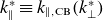 $k_\parallel ^* \equiv k_{\parallel ,\mathrm{CB}}(k_\perp ^*)$
, is the largest parallel wavenumber reached by the energy cascade within the inertial range. A depiction of
$k_\parallel ^* \equiv k_{\parallel ,\mathrm{CB}}(k_\perp ^*)$
, is the largest parallel wavenumber reached by the energy cascade within the inertial range. A depiction of $\mathcal{E}_{\delta B}(k_\perp , k_\parallel )$
that includes
$\mathcal{E}_{\delta B}(k_\perp , k_\parallel )$
that includes $k_\perp ^*$
,
$k_\perp ^*$
, $k_\parallel ^*$
and the function
$k_\parallel ^*$
and the function $k_{\parallel ,\mathrm{CB}}(k_\perp )$
is shown in figure 3(a).
$k_{\parallel ,\mathrm{CB}}(k_\perp )$
is shown in figure 3(a).
3.2. Quasi-linear focusing near the turbulent transition range
Let us ignore for a moment the expansion of the solar wind and focus on how the presence of the turbulent transition range bounds the regions of wave vector space and velocity space where wave–particle interactions lead to PICW emission via quasi-linear focusing. Relative to the inertial range, there is vanishingly little power in the transition range. Indeed, observations of imbalanced turbulence by PSP have shown that the spectral energy across the transition range drops by at least a factor of $100$
(Bowen et al. Reference Bowen2022, Reference Bowen, Bale, Chandran, Chasapis, Chen, Dudok de Wit, Mallet, Meyrand and Squire2024a
). Let us assume for the sake of simplicity that the power in the oblique ICW spectrum falls to zero for
$100$
(Bowen et al. Reference Bowen2022, Reference Bowen, Bale, Chandran, Chasapis, Chen, Dudok de Wit, Mallet, Meyrand and Squire2024a
). Let us assume for the sake of simplicity that the power in the oblique ICW spectrum falls to zero for $k_\perp \gt k_\perp ^*$
and
$k_\perp \gt k_\perp ^*$
and $k_\parallel \gt k_\parallel ^*$
. The highest-frequency oblique ICWs in the inertial range, depicted by the red circle in figure 3(a), dominate the oblique-ICW heating rate.
$k_\parallel \gt k_\parallel ^*$
. The highest-frequency oblique ICWs in the inertial range, depicted by the red circle in figure 3(a), dominate the oblique-ICW heating rate.
The negligible power in oblique ICWs at $k_\parallel \gtrsim k_\parallel ^*$
restricts strong cyclotron-resonant interactions between protons and oblique ICWs to
$k_\parallel \gtrsim k_\parallel ^*$
restricts strong cyclotron-resonant interactions between protons and oblique ICWs to $v_\parallel \lesssim v_\parallel ^*$
, where
$v_\parallel \lesssim v_\parallel ^*$
, where
 \begin{align} v_\parallel ^*=v_{\parallel \mathrm{res,O}}\big(k_\parallel ^*, 1\big)=\dfrac {\omega _{k_\parallel {\mathrm{r,O}}}(k_\parallel ^*)-\varOmega _{\mathrm{p}}}{k_\parallel ^*} \end{align}
is the solution to (2.4) for oblique ICWs at the start of the transition range. We note that $v_\parallel ^* \lt 0$
, so faster protons moving in the direction opposite the wave-propagation direction can resonate, but slower protons cannot. We plot
$v_\parallel ^* \lt 0$
, so faster protons moving in the direction opposite the wave-propagation direction can resonate, but slower protons cannot. We plot $v_\parallel ^*$
with a vertical dashed black line over a model proton velocity distribution in figure 3(b). Let us assume the resonant heating by the oblique cascade is sufficiently strong to flatten the proton distribution constant along the quasi-linear contours of (2.5) for oblique ICWs at
$v_\parallel ^*$
with a vertical dashed black line over a model proton velocity distribution in figure 3(b). Let us assume the resonant heating by the oblique cascade is sufficiently strong to flatten the proton distribution constant along the quasi-linear contours of (2.5) for oblique ICWs at $v_\parallel \lt v_\parallel ^\ast$
. For
$v_\parallel \lt v_\parallel ^\ast$
. For $v_\parallel \gt v_\parallel ^*$
, we assume the proton distribution has not been extensively heated by oblique ICWs and is significantly more isotropic than for
$v_\parallel \gt v_\parallel ^*$
, we assume the proton distribution has not been extensively heated by oblique ICWs and is significantly more isotropic than for $v_\parallel \lt v_\parallel ^*$
. We depict the resulting distribution in figure 3(b). As discussed in § 2.3, the proton distribution for
$v_\parallel \lt v_\parallel ^*$
. We depict the resulting distribution in figure 3(b). As discussed in § 2.3, the proton distribution for $v_\parallel \lt v_\parallel ^*$
is resonantly unstable to PICWs.
$v_\parallel \lt v_\parallel ^*$
is resonantly unstable to PICWs.
The resonance condition (2.3), now applied to the relevant $n=1$
cyclotron resonance for PICWs, is
$n=1$
cyclotron resonance for PICWs, is
 \begin{align} \omega _{k_\parallel {\mathrm{r,P}}}(k_\parallel )=k_\parallel v_\parallel +\varOmega _{\mathrm{p}}. \end{align}
Solutions to (3.2) are easily found pictorially in a resonance diagram, which we have included in figure 3(c). We plot the PICW frequency $\omega _{k_\parallel {\mathrm{r,P}}}$
, the left-hand side of (3.2), versus
$\omega _{k_\parallel {\mathrm{r,P}}}$
, the left-hand side of (3.2), versus $k_\parallel$
with a solid black line. The right-hand side of (3.2) is a straight line originating from the top-left corner of the plot. As discussed in § 2.3, the point at which the two lines intersect is a solution of the resonance condition. We have included two lines for two different parallel velocities. The slanted dashed line is
$k_\parallel$
with a solid black line. The right-hand side of (3.2) is a straight line originating from the top-left corner of the plot. As discussed in § 2.3, the point at which the two lines intersect is a solution of the resonance condition. We have included two lines for two different parallel velocities. The slanted dashed line is $k_\parallel v_\parallel ^*+\varOmega _{\mathrm{p}}$
, which intersects
$k_\parallel v_\parallel ^*+\varOmega _{\mathrm{p}}$
, which intersects $\omega _{k_\parallel {\mathrm{r,P}}}$
at
$\omega _{k_\parallel {\mathrm{r,P}}}$
at
 \begin{align} k_{\parallel {\mathrm{P}}}^*=k_{\parallel {\mathrm{P}}}\big(v_\parallel ^*\big), \end{align}
the parallel wavenumber for PICWs resonant with protons with $v_\parallel =v_\parallel ^*$
. We illustrate the value of
$v_\parallel =v_\parallel ^*$
. We illustrate the value of $k_{\parallel {\mathrm{P}}}^*$
with a black dashed vertical line in figure 3(c). The blue solid line in figure 3(c) is
$k_{\parallel {\mathrm{P}}}^*$
with a black dashed vertical line in figure 3(c). The blue solid line in figure 3(c) is $k_\parallel v_\parallel +\varOmega _{\mathrm{p}}$
for a parallel velocity
$k_\parallel v_\parallel +\varOmega _{\mathrm{p}}$
for a parallel velocity $v_\parallel \lt v_\parallel ^*$
, which is itself shown by the vertical solid blue line in figure 3(b). The blue solid line in figure 3(c) intersects the wave frequency at a parallel wavenumber
$v_\parallel \lt v_\parallel ^*$
, which is itself shown by the vertical solid blue line in figure 3(b). The blue solid line in figure 3(c) intersects the wave frequency at a parallel wavenumber $k_\parallel \lt k_{\parallel {\mathrm{P}}}^*$
, where PICWs are unstable. This blue solid line is coloured this way to represent an unstable PICW actively cooling the plasma. Although our discussion so far has focused on a single wave mode, we expect PICW emission will occur in a band of wavenumbers at
$k_\parallel \lt k_{\parallel {\mathrm{P}}}^*$
, where PICWs are unstable. This blue solid line is coloured this way to represent an unstable PICW actively cooling the plasma. Although our discussion so far has focused on a single wave mode, we expect PICW emission will occur in a band of wavenumbers at $k_\parallel \lesssim k_{\parallel {\mathrm{P}}}^*$
, as depicted by the blue circle in figure 3(a).
$k_\parallel \lesssim k_{\parallel {\mathrm{P}}}^*$
, as depicted by the blue circle in figure 3(a).
What about PICWs with $k_\parallel \gt k_{\parallel {\mathrm{P}}}^*$
? In our resonance diagram, these waves would be represented by lines that are shallower than the black dashed line. Shallower lines correspond to resonances with protons that have
$k_\parallel \gt k_{\parallel {\mathrm{P}}}^*$
? In our resonance diagram, these waves would be represented by lines that are shallower than the black dashed line. Shallower lines correspond to resonances with protons that have $v_\parallel \gt v_\parallel ^*$
. Thus, PICWs with
$v_\parallel \gt v_\parallel ^*$
. Thus, PICWs with $k_\parallel \gt k_{\parallel {\mathrm{P}}}^*$
are strongly damped by the proton distribution. The result of quasi-linear focusing is therefore very little wave energy for
$k_\parallel \gt k_{\parallel {\mathrm{P}}}^*$
are strongly damped by the proton distribution. The result of quasi-linear focusing is therefore very little wave energy for $k_\parallel \gt k_{\parallel {\mathrm{P}}}^*$
and a continuous buildup of PICW energy for
$k_\parallel \gt k_{\parallel {\mathrm{P}}}^*$
and a continuous buildup of PICW energy for $k_\parallel \lt k_{\parallel {\mathrm{P}}}^*$
. In a homogeneous plasma, there is no linear mechanism by which the wave energy at
$k_\parallel \lt k_{\parallel {\mathrm{P}}}^*$
. In a homogeneous plasma, there is no linear mechanism by which the wave energy at $k_\parallel \lt k_{\parallel {\mathrm{P}}}^*$
can be transported to
$k_\parallel \lt k_{\parallel {\mathrm{P}}}^*$
can be transported to $k_\parallel \gt k_{\parallel {\mathrm{P}}}^*$
, where the wave energy can damp and heat the plasma. As it turns out, such a transport mechanism is the natural consequence of the WKB propagation of PICWs in the inhomogeneous solar wind.
$k_\parallel \gt k_{\parallel {\mathrm{P}}}^*$
, where the wave energy can damp and heat the plasma. As it turns out, such a transport mechanism is the natural consequence of the WKB propagation of PICWs in the inhomogeneous solar wind.
3.3. The WKB evolution of PICWs
We now detail how the propagation and advection of PICWs in the inhomogeneous solar wind change the properties of the waves and, inevitably, lead to their dissipation. As PICWs are driven unstable by the turbulent cascade, they will both propagate and be advected anti-sunward. Let us assume that the solar-wind background is in steady state. Then, the real part of the angular frequency of PICWs, measured in the heliocentric frame, will be constant with radius:
 \begin{align} \omega _{{\mathrm{r}}\odot }=k_\parallel U+\omega _{k_\parallel {\mathrm{r}},P}= {\mathrm{const}}. \end{align}
In the $U\gg v_{\mathrm{A}}$
super-Alvénic wind,
$U\gg v_{\mathrm{A}}$
super-Alvénic wind, $\omega _{k_\parallel {\mathrm{r,P}}}\leqslant k_\parallel v_{\mathrm{A}}\ll k_\parallel U$
, and so
$\omega _{k_\parallel {\mathrm{r,P}}}\leqslant k_\parallel v_{\mathrm{A}}\ll k_\parallel U$
, and so $\omega _{{\mathrm{r}}\odot }=\omega _{k_\parallel {\mathrm{r,P}}}+k_\parallel U\simeq k_\parallel U$
. For heliocentric distances much larger than the Alfvén critical point,
$\omega _{{\mathrm{r}}\odot }=\omega _{k_\parallel {\mathrm{r,P}}}+k_\parallel U\simeq k_\parallel U$
. For heliocentric distances much larger than the Alfvén critical point, $U\sim {\mathrm{const.}}$
, so
$U\sim {\mathrm{const.}}$
, so $k_\parallel \sim {\mathrm{const}}$
. Thus,
$k_\parallel \sim {\mathrm{const}}$
. Thus, $k_\parallel d_{\mathrm{p}}\sim n^{-1/2}\sim x$
, where
$k_\parallel d_{\mathrm{p}}\sim n^{-1/2}\sim x$
, where $x=r/R_{\odot }$
is the heliocentric distance normalised to the solar radius
$x=r/R_{\odot }$
is the heliocentric distance normalised to the solar radius $R_{\odot }$
. In the sub-Alfvénic wind, the same analysis, again taking the non-dispersive limit, yields
$R_{\odot }$
. In the sub-Alfvénic wind, the same analysis, again taking the non-dispersive limit, yields $k_\parallel v_{\mathrm{A}}\sim {\mathrm{const.}}$
, so
$k_\parallel v_{\mathrm{A}}\sim {\mathrm{const.}}$
, so $k_\parallel d_{\mathrm{p}}\sim B^{-1}\sim x^2$
at least for
$k_\parallel d_{\mathrm{p}}\sim B^{-1}\sim x^2$
at least for $x\gtrsim 3$
. While the radial scaling of
$x\gtrsim 3$
. While the radial scaling of $U$
near the Alfvén critical point somewhat complicates the preceding analysis, the general qualitative conclusion is clear: the normalised parallel wavenumber,
$U$
near the Alfvén critical point somewhat complicates the preceding analysis, the general qualitative conclusion is clear: the normalised parallel wavenumber, $k_\parallel d_{\mathrm{p}}$
, of PICWs increases as the waves travel away from the Sun.
$k_\parallel d_{\mathrm{p}}$
, of PICWs increases as the waves travel away from the Sun.
Depicted diagrammatically, the radial evolution of $\omega _{k_\parallel {\mathrm{r,P}}}/\varOmega _{\mathrm{p}}$
and
$\omega _{k_\parallel {\mathrm{r,P}}}/\varOmega _{\mathrm{p}}$
and $k_\parallel d_{\mathrm{p}}$
is very simple because the PICW cold-plasma dispersion relation (2.2) is invariant with heliocentric distance if
$k_\parallel d_{\mathrm{p}}$
is very simple because the PICW cold-plasma dispersion relation (2.2) is invariant with heliocentric distance if $\omega _{k_\parallel {\mathrm{r,P}}}$
and
$\omega _{k_\parallel {\mathrm{r,P}}}$
and $k_\parallel$
are normalised by
$k_\parallel$
are normalised by $\varOmega _{\mathrm{p}}$
and
$\varOmega _{\mathrm{p}}$
and $d_{\mathrm{p}}$
, respectively. As a result, the normalised frequency and parallel wavenumber of a given PICW simply increase along the normalised dispersion relation as the waves are transported to larger radii. We depict this evolution with a black arrow in figure 4(c) and vertical black arrow in figure 4(a). As
$d_{\mathrm{p}}$
, respectively. As a result, the normalised frequency and parallel wavenumber of a given PICW simply increase along the normalised dispersion relation as the waves are transported to larger radii. We depict this evolution with a black arrow in figure 4(c) and vertical black arrow in figure 4(a). As $k_\parallel d_{\mathrm{p}}$
increases, the resonant parallel velocity decreases, as depicted by the shallower red resonance line in figure 4(c). If PICW emission and absorption occur continuously across a range of heliocentric distances, then at any given heliocentric distance one will observe PICWs cooling protons with
$k_\parallel d_{\mathrm{p}}$
increases, the resonant parallel velocity decreases, as depicted by the shallower red resonance line in figure 4(c). If PICW emission and absorption occur continuously across a range of heliocentric distances, then at any given heliocentric distance one will observe PICWs cooling protons with $v_\parallel \lt v_\parallel ^*$
and heating protons with
$v_\parallel \lt v_\parallel ^*$
and heating protons with $v_\parallel ^*\lt v_\parallel \lt 0$
, as shown in figure 4(b). This distinct heating signature was recently produced by a quasi-linear analysis of PICWs observed by PSP during an encounter with a fast solar-wind stream (Bowen et al. Reference Bowen2024b
).
$v_\parallel ^*\lt v_\parallel \lt 0$
, as shown in figure 4(b). This distinct heating signature was recently produced by a quasi-linear analysis of PICWs observed by PSP during an encounter with a fast solar-wind stream (Bowen et al. Reference Bowen2024b
).
4. Conclusion
In this work, we have shown that observations of heating by PICWs in the fast solar wind can be explained by a continuous process of PICW emission, propagation and absorption that we call cyclotron breaking. The name ‘cyclotron breaking’ comes as an analogy to water waves breaking on the shore. In the same way that water waves can be driven by a shoreward wind interacting with the surface of the water, PICWs can be driven by the turbulent cascade of anti-sunward Alfvén waves interacting with the proton distribution. Both waves then propagate in an inhomogeneous medium: the water waves in increasingly shallower water as they approach the shore, and PICWs in increasingly rarefied plasma as they are transported away from the Sun. As they propagate, the wavelength and frequency of both waves evolve such that the waves go from gaining in amplitude to dissipating their energy. In the case of water waves, the waveform itself undergoes nonlinear steepening as it moves up the shore, eventually reaching a point where the wave breaks and turbulently dissipates. On the other hand, PICWs evolve from resonating with relatively fast protons, to which they are unstable, to resonating with relatively slow protons, on which they damp. While the PICW damping described by this process is purely linear, we nevertheless borrow the concept of wave breaking here as a metaphorical comparison.
Parallel ICWs driven unstable by quasi-linear focusing in the vicinity of the turbulent transition range cool the solar wind (see figure 3). The PICWs that are at one radius unstable will propagate away from the Sun. As they do, the wave frequency and parallel wave vector will evolve according to (3.4), i.e. along the (properly normalised) PICW dispersion relation towards larger values, as shown by the arrow in (c). The solution to the resonance condition changes appropriately, with PICWs resonating with slower and slower protons as they propagate – shown by the red line in (b). At some point in their anti-sunward trajectory, the PICWs will begin to resonate with the $v_\parallel \gt v_\parallel ^*$
part of the proton velocity distribution (which has not been heated by the ICW cascade) and will be damped. The damped waves heat the solar wind, as emphasised by the red lines in (b, c). We also approximate the wavenumber spectrum of damped PICWs with a red circle at
$v_\parallel \gt v_\parallel ^*$
part of the proton velocity distribution (which has not been heated by the ICW cascade) and will be damped. The damped waves heat the solar wind, as emphasised by the red lines in (b, c). We also approximate the wavenumber spectrum of damped PICWs with a red circle at $k_\parallel \gtrsim k_\parallel ^*$
in (a).
$k_\parallel \gtrsim k_\parallel ^*$
in (a).

Cyclotron breaking is reminiscent of the sweeping scenario, in which it is hypothesised that the Sun launches kilohertz-range ICWs (Axford & McKenzie Reference Axford and McKenzie1992) that damp as they propagate away from the Sun. The damping of these waves occurs at a heliocentric distance at which the wave frequency is comparable to the local cyclotron frequency, which is a radially decreasing function of heliocentric distance (Schwartz, Feldman & Gary Reference Schwartz, Feldman and Gary1981; Tu & Marsch Reference Tu and Marsch1997). The cyclotron frequency thus ‘sweeps’ down through the wave power spectrum, damping out the waves first at high frequencies near the Sun and then at lower frequencies as $r$
increases. A difference between sweeping and cyclotron breaking is that in the sweeping scenario the PICWs are generated at the Sun, whereas in cyclotron breaking they are generated in the solar wind via quasi-linear focusing of oblique ICWs that are produced locally by the turbulent cascade. Cyclotron breaking therefore mitigates many of the observational inconsistencies with the solar origin of ICWs in the sweeping model (Cranmer Reference Cranmer2000, Reference Cranmer2001; Hollweg Reference Hollweg2000).
$r$
increases. A difference between sweeping and cyclotron breaking is that in the sweeping scenario the PICWs are generated at the Sun, whereas in cyclotron breaking they are generated in the solar wind via quasi-linear focusing of oblique ICWs that are produced locally by the turbulent cascade. Cyclotron breaking therefore mitigates many of the observational inconsistencies with the solar origin of ICWs in the sweeping model (Cranmer Reference Cranmer2000, Reference Cranmer2001; Hollweg Reference Hollweg2000).
The unique heating signature predicted by cyclotron breaking – PICWs cooling relatively fast protons while heating relatively slow protons – is consistent with heating signatures produced by quasi-linear analysis of PICW heating in the fast solar wind (Bowen et al. Reference Bowen2024b ). The same analysis, however, also found that PICWs on average heat the solar wind. It is not yet established under what conditions cyclotron breaking can explain this result. Net heating will occur at a given heliocentric distance when the PICW power being absorbed is greater than the PICW power being emitted. If PICWs are driven unstable at a specific heliocentric distance, they will only begin to damp once they have propagated away from where they were driven unstable. It is intuitively clear that these waves can on average heat the solar wind at heliocentric distances larger than where they were emitted because there is no local PICW emission to offset the damping of the waves.
For a process of continuous PICW emission and absorption more akin to what is observed in the solar wind (Bowen et al. Reference Bowen2024b
), determining the balance between local heating and cooling at a given heliocentric distance is a non-trivial task. To do this properly, a more comprehensive modelling effort will need to be undertaken in which the radial evolution of $v_\parallel ^*$
,
$v_\parallel ^*$
, $k_{\parallel {\mathrm{P}}}^*$
and PICW wave amplitude are treated self-consistently. Broadly speaking, however, one can imagine that if the incident flux of PICWs with
$k_{\parallel {\mathrm{P}}}^*$
and PICW wave amplitude are treated self-consistently. Broadly speaking, however, one can imagine that if the incident flux of PICWs with $k_\parallel \gt k_{\parallel {\mathrm{P}}}^*$
is sufficiently large – and that their damping is sufficiently strong – local heating will dominate local cooling. So long as the power emitted as PICWs decreases sufficiently quickly as a function of radius, this condition may well be satisfied. Indeed, Bowen et al. (Reference Bowen2024b
) found that the PICW heating rate decreased rapidly with heliocentric distance,
$k_\parallel \gt k_{\parallel {\mathrm{P}}}^*$
is sufficiently large – and that their damping is sufficiently strong – local heating will dominate local cooling. So long as the power emitted as PICWs decreases sufficiently quickly as a function of radius, this condition may well be satisfied. Indeed, Bowen et al. (Reference Bowen2024b
) found that the PICW heating rate decreased rapidly with heliocentric distance, ${\sim }x^{-a}$
with
${\sim }x^{-a}$
with $4\lt a\lt 5$
, so it appears plausible that cyclotron breaking can explain observations of net heating by PICWs in the young, fast solar wind.
$4\lt a\lt 5$
, so it appears plausible that cyclotron breaking can explain observations of net heating by PICWs in the young, fast solar wind.
Acknowledgements
We would like to thank M. Kunz, J. Squire, M. Zhang, K. Klein, N. Sioulas, C. Chen, N. Shankarappa, L. Wilson, T. Adkins and the participants of the Parker Four conference, whose comments and conversations helped refine this work.
Editor Thierry Passot thanks the referees for their advice in evaluating this article.
Funding
This work was supported by NASA grants 80NSSC24K0171 and NNN06AA01C and DOE award DE-SC0026201.
Declaration of interests
The authors report no conflict of interest.
Appendix A. Proof that $\omega _{k{\mathrm{r}}}\gt \omega _{k_\parallel {\mathrm{r}}}$
for all
$(k_\parallel ,k_\perp )\gt 0$
$\omega _{k{\mathrm{r}}}\gt \omega _{k_\parallel {\mathrm{r}}}$
for all
$(k_\parallel ,k_\perp )\gt 0$


Let us prove that $\omega _{k{\mathrm{r}}}\gt \omega _{k_\parallel {\mathrm{r}}}$
for all
$\omega _{k{\mathrm{r}}}\gt \omega _{k_\parallel {\mathrm{r}}}$
for all $(k_\parallel ,k_\perp )\gt 0$
. If
$(k_\parallel ,k_\perp )\gt 0$
. If $\omega _{k{\mathrm{r}}}\gt \omega _{k_\parallel {\mathrm{r}}}$
, then, noting that
$\omega _{k{\mathrm{r}}}\gt \omega _{k_\parallel {\mathrm{r}}}$
, then, noting that $\omega _{k{\mathrm{r}}}\gt 0$
and
$\omega _{k{\mathrm{r}}}\gt 0$
and $\omega _{k_\parallel {\mathrm{r}}}\gt 0$
by definition,
$\omega _{k_\parallel {\mathrm{r}}}\gt 0$
by definition, $2\tilde {\omega }_{k{\mathrm{r}}}^2\gt 2\tilde {\omega }_{k_\parallel {\mathrm{r}}}^2$
, where
$2\tilde {\omega }_{k{\mathrm{r}}}^2\gt 2\tilde {\omega }_{k_\parallel {\mathrm{r}}}^2$
, where $\tilde {\omega }_{k{\mathrm{r}}}=\omega _{k{\mathrm{r}}}/\varOmega _{\mathrm{p}}$
and
$\tilde {\omega }_{k{\mathrm{r}}}=\omega _{k{\mathrm{r}}}/\varOmega _{\mathrm{p}}$
and $\tilde {\omega }_{k_\parallel {\mathrm{r}}}=\omega _{k_\parallel {\mathrm{r}}}/\varOmega _{\mathrm{p}}$
. Using the dispersion relation (2.1) and rearranging, the inequality becomes
$\tilde {\omega }_{k_\parallel {\mathrm{r}}}=\omega _{k_\parallel {\mathrm{r}}}/\varOmega _{\mathrm{p}}$
. Using the dispersion relation (2.1) and rearranging, the inequality becomes
 \begin{align} b_{\mathrm{O}}-b_{\mathrm{P}}\gt \sqrt {d_{\mathrm{O}}}-\sqrt {d_{\mathrm{P}}}, \end{align}
where $d_{\mathrm{O/P}}=b_{\mathrm{O/P}}^2-4c_{\mathrm{O/P}}$
,
$d_{\mathrm{O/P}}=b_{\mathrm{O/P}}^2-4c_{\mathrm{O/P}}$
, $b_{\mathrm{O}}=b_{\mathrm{P}}+\tilde {k}_{\perp }^2(1+\tilde {k}_{\parallel }^2)$
,
$b_{\mathrm{O}}=b_{\mathrm{P}}+\tilde {k}_{\perp }^2(1+\tilde {k}_{\parallel }^2)$
,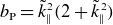 $b_{\mathrm{P}}=\tilde {k}_{\parallel }^2(2+\tilde {k}_{\parallel }^2)$
,
$b_{\mathrm{P}}=\tilde {k}_{\parallel }^2(2+\tilde {k}_{\parallel }^2)$
, $c_{\mathrm{O}}=c_{\mathrm{P}}+\tilde {k}_{\parallel }^2\tilde {k}_{\perp }^2$
,
$c_{\mathrm{O}}=c_{\mathrm{P}}+\tilde {k}_{\parallel }^2\tilde {k}_{\perp }^2$
, $c_{\mathrm{P}}=\tilde {k}_{\parallel }^4$
,
$c_{\mathrm{P}}=\tilde {k}_{\parallel }^4$
, $\tilde {k}_{\parallel }=k_\parallel d_{\mathrm{p}}$
and
$\tilde {k}_{\parallel }=k_\parallel d_{\mathrm{p}}$
and $\tilde {k}_{\perp }=k_\perp d_{\mathrm{p}}$
. Using the above definitions, one can show that
$\tilde {k}_{\perp }=k_\perp d_{\mathrm{p}}$
. Using the above definitions, one can show that
 \begin{align} d_{\mathrm{O}}&=d_{\mathrm{P}}+\tilde {k}_{\perp }^4\big(1+\tilde {k}_{\parallel }^2\big)^2+2\tilde {k}_{\perp }^2\tilde {k}_{\parallel }^4\big(3+\tilde {k}_{\parallel }^2\big),\\[-10pt]\nonumber \end{align}
 \begin{align} d_{\mathrm{P}}&=\tilde {k}_{\parallel }^6\big(4+\tilde {k}_{\parallel }^2\big). \end{align}
Thus $b_{\mathrm{O}}\gt b_{\mathrm{P}}\gt 0$
and
$b_{\mathrm{O}}\gt b_{\mathrm{P}}\gt 0$
and $d_{\mathrm{O}}\gt d_{\mathrm{P}}\gt 0$
, so both sides of (A1) can be squared with the inequality maintained. After some simplification, one finds
$d_{\mathrm{O}}\gt d_{\mathrm{P}}\gt 0$
, so both sides of (A1) can be squared with the inequality maintained. After some simplification, one finds
 \begin{align} \sqrt {d_{\mathrm{O}}d_{\mathrm{P}}}\gt d_{\mathrm{P}} + \tilde {k}_{\perp }^2\tilde {k}_{\parallel }^4\big(3+\tilde {k}_{\parallel }^2\big). \end{align}
As before, both sides of the inequality are positive and can be squared with the inequality intact. After substituting (A2a ), a number of terms drop out and the inequality becomes
 \begin{align} k_\perp ^4\big[d_{\mathrm{P}}\big(1+\tilde {k}_{\parallel }^2\big)^2-\tilde {k}_{\parallel }^8\big(3+\tilde {k}_{\parallel }^2\big)^2\big]\gt 0. \end{align}
Upon substituting (A2b ) and simplifying, one is left with
 \begin{align} \tilde {k}_{\perp }^4\tilde {k}_{\parallel }^6\gt 0, \end{align}
which is indeed satisfied for all $(k_\parallel ,k_\perp )\gt (0,0)$
. QED.
$(k_\parallel ,k_\perp )\gt (0,0)$
. QED.


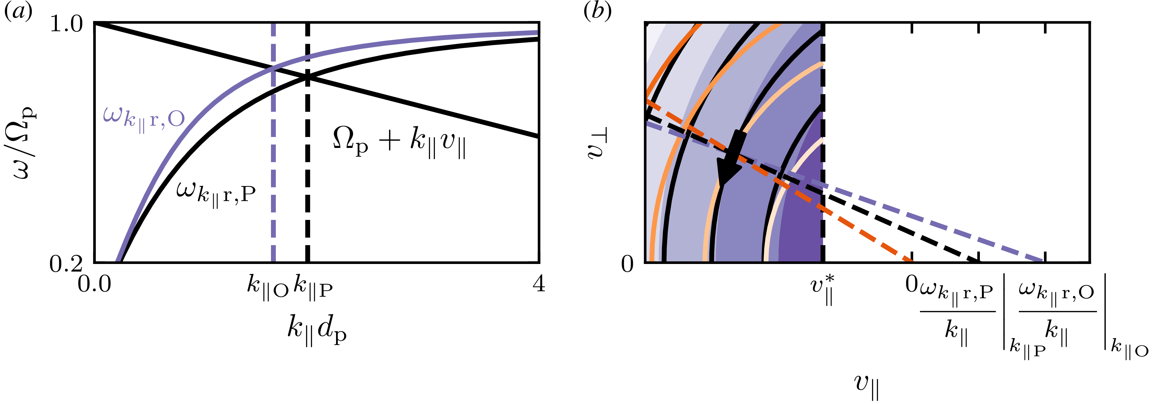
 ωk∥r,O
 k⊥dp=10
 ωk∥r,P
 k∥
k∥ k∥P>k∥O
 ωkr,O
ωkr,O ωk∥r,P
 Ωp+k∥v∥
 (ωk∥r,O/k∥)|k∥O−(ωk∥r,P/k∥)|k∥P>0
 v∥
v∥ v∥∗
v∥∗ (ωk∥r,O/k∥)|k∥O−(ωk∥r,P/k∥)|k∥P>0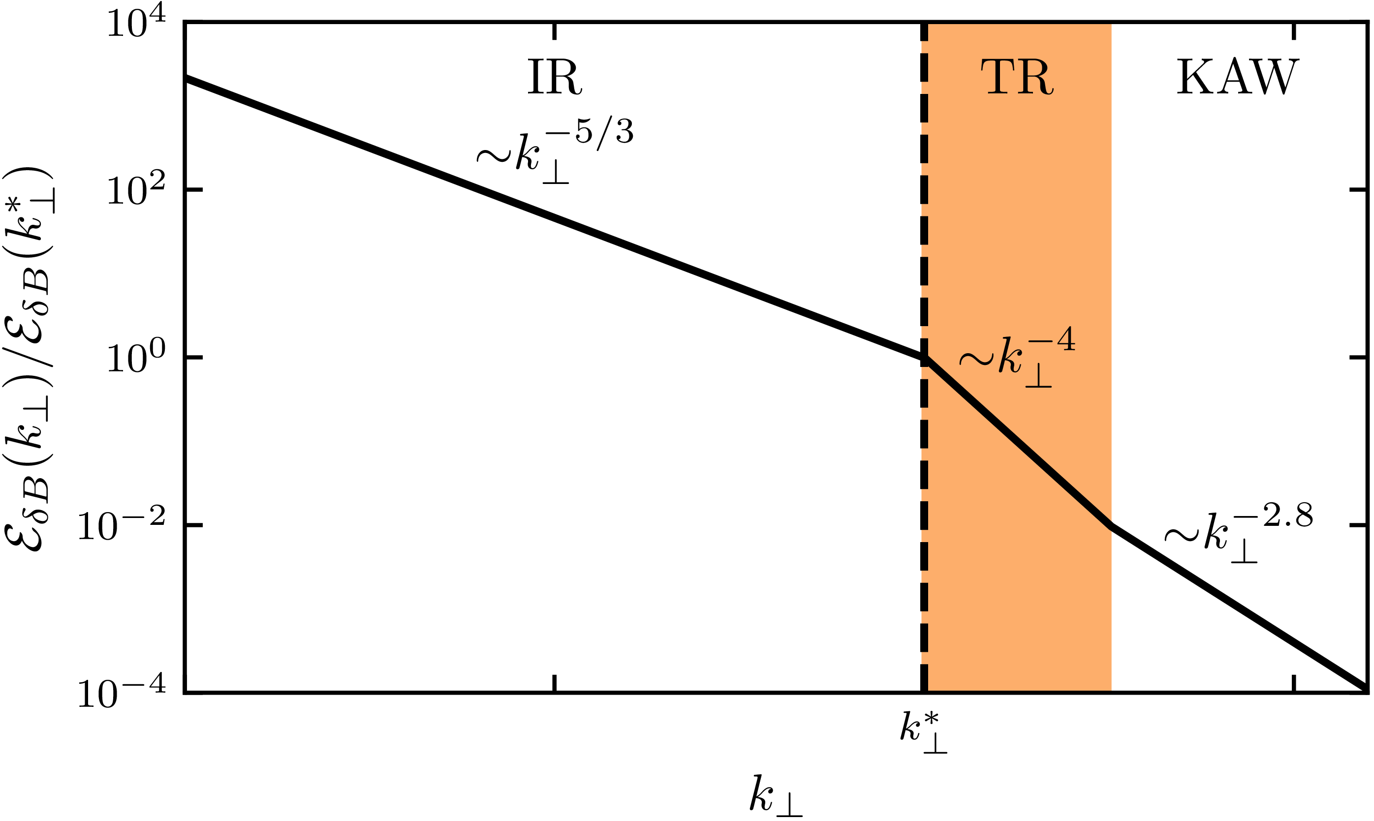
 EδB(k⊥)
 ∼k⊥−4
∼k⊥−4 k⊥∗
k⊥∗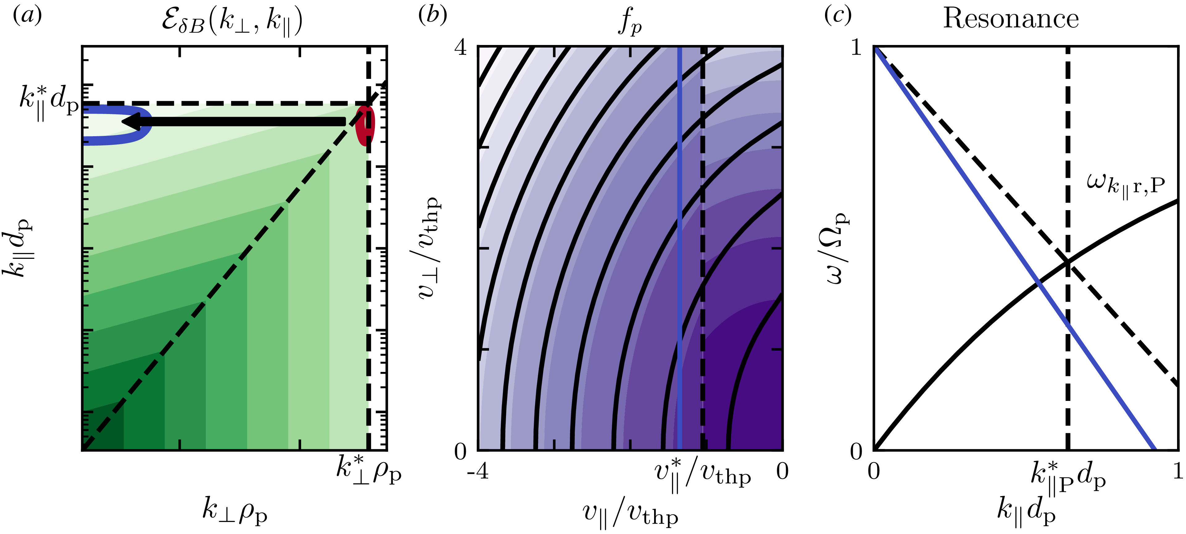
 δB
δB k⊥∗
k⊥∗ k∥∗
k∥∗ k∥,CB(k⊥)
 fp
fp v∥
v∥ v∥∗
v∥∗ k∥=k∥∗
 k⊥=k⊥∗
 fp
fp fp
fp v∥>v∥∗
 fp
fp fp
fp v∥
v∥ k∥
k∥ ωk∥r,P
 k∥
k∥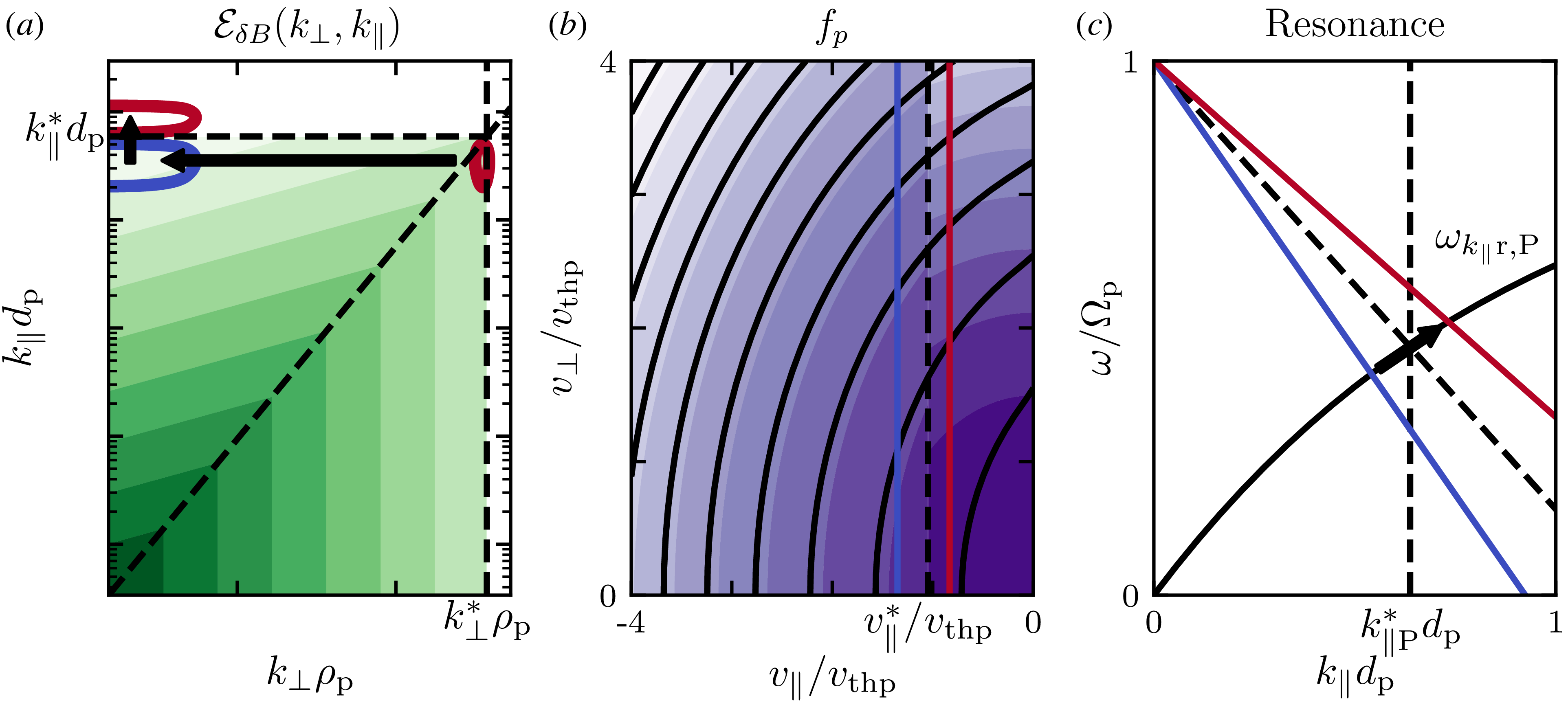
 v∥>v∥∗
 k∥≳k∥∗
 Open access

