





Introduction
The ever-increasing demands for high data rates, high bandwidth, and improved resolution drive forward the constant advancements in the millimeter-wave (mm-wave) technology. Innovations in communication technologies have enabled the industry to create and deploy highly reliable and robust systems. Research on 5G and 6G networks pushes the evolution of modern wired and wireless communications. But as the conventional spectrum becomes increasingly congested, next-generation emerging 6G architectures are turning toward the millimeter-wave region to unlock new performance frontiers. Among these, the D-band ( $110-170\,\mathrm{GHz}$), due to its high available bandwidth, has especially become promising for various applications such as high-resolution imaging, advanced radar systems, and high-speed wired and wireless communications [Reference Aslam, Wilcher, Chatterjee, Yoon, Arnold and Sinha1]. The semiconductor industry with its efficient miniaturization techniques has enabled the usage of D-band to develop highly compact systems at potentially low costs [Reference Pallotta, Roux, Del Rio, Sevillano, Pirbazari, Mazzanti, Ermolov, Lamminen, Säily, Frecassetti, Moretto and De Cos2].
For such efficient communication systems in D-band frequencies, the key performance always lies in the optimal design of the individual components, such as the transceivers, transmission lines, antennas, etc. In recent times, a lot of research is being carried out at component level like antenna designs in [Reference De Kok, Smolders and Johannsen3] or CMOS transceiver designs [Reference Xu, Gu, Wu and Chang4] and [Reference Karakuzulu, Eissa, Kissinger and Malignaggi5]. This research leads to the development of very high data-rate transmission links [Reference D’heer and Reynaert6–Reference Vassilev, He, Carpenter, Zirath, Yan, Hassona, Bao, Emanuelsson, Chen, Hörberg, Li and Hansrydl8]. Not only in links, but the advancements have also bloomed up to system-level developments on high-resolution radar sensing in this range [Reference Stadler, Papurcu, Welling, Tejero Alfageme and Pohl9–Reference Baer, Schulz, Rolfes and Musch11].
Although there is a constant advancement in the development of high-frequency technologies, they still face some practical limitations. At millimeter-wave range, signals experience significant attenuation in wired links and substantial free-space path loss in wireless channels. Although the planar transmission lines and the traditional metallic waveguides are well established, they become less suitable at these frequencies because they introduce considerable losses or occupy too much physical space, and are not cost-effective for long-distance connections. These constraints highlight the strong need for further development of systems that offer lower loss for wired links and at the same time offer antenna solutions that are capable of providing higher gain for wireless systems. Needless to say that combining both approaches can lead to more compact, efficient, and economically viable designs for next-generation communication platforms.
Pertaining to low-loss transmission lines, radio-over-fiber technology presents a promising solution. It involves transmitting high-frequency electromagnetic (EM) waves through polymer fibers acting as dielectric waveguides (DWGs). These DWGs are typically fabricated from low-cost polymer materials such as Polyethylene (PE), Polystyrene (PS), or Polytetrafluoroethylene (PTFE). These DWGs are not only more economical and low-loss but also do offer mechanical flexibility up to a certain extent. This gives them an upper edge in comparison to their metallic counterparts. This advantage is widely exploited in this work as well. The available research on DWGs for mm-wave frequencies enables one to easily design and incorporate DWGs into systems as per requirement [Reference Yeh and Shimabukuro12–Reference Schneider15]. When optimized, they can exhibit even lower attenuation compared to conventional metallic waveguides [Reference Schneider and Meyer16]. For point-to-point D-band wired links, the advantages of DWGs make them a great alternative [Reference Vaes, Dens, Ducournau and Reynaert17, Reference Dens, Vaes, Ooms, Wagner and Reynaert18]. However, for wireless systems, to mitigate the high free space path loss (approx.  $75\,\mathrm{dB}$ for a one-meter link at a frequency of $125\,\mathrm{GHz}$), high-gain antennas are also needed. In this context, a lens antenna is a promising solution that offers high gain and good aperture efficiency [Reference Thornton and Huang19]. In addition, they offer cost efficiency and seamless integration into complex systems.
This work seeks to combine the strengths of low-loss DWG links and high-gain lens antennas through an integrated design approach. The possibilities are explored where one can combine the advantages of both and put them together as one plug-n-play system. Prior studies have explored a range of lens geometries including convex, elliptical, hemispherical, and hemi-elliptical typically mounted on low-gain patch antennas or metallic waveguide apertures, as reported in [Reference Bisognin, Titz, Luxey, Jacquemod, Ferrero, Lugara, Pilard, Gianesello, Gloria, Costa, Laporte, Ezzeddine, Lima and Fernandes20] and [Reference Pohl21], respectively. However, directly feeding such lenses with DWGs could not only enhance overall performance but also add on a mechanical flexibility via the DWGs. This idea could be exploited into designing various system applications. For example, the flexible nature of DWGs allows lens antennas to be positioned at various locations (potentially away from the transceiver) or oriented in different directions [Reference Baer, Schulz, Rolfes and Musch11, Reference Geiger, Hitzler, Iberle and Waldschmidt22, Reference Geiger, Grüner, Fischer, Durr, Chaloun and Waldschmidt27]. This flexibility opens up new possibilities for measurement setups and improves the functionality of D-band radar and communication systems.
This study encompasses the design, performance, and practical considerations of such a lens antenna. The antenna is fed by a circular dielectric waveguide (CDWG) and the design is optimized for operation in the  $115-130\,\mathrm{GHz}$ frequency range. This frequency range has recently been gaining attention and considerable interest for advanced short-range radar system applications (especially at $122\,\mathrm{GHz}$). Since the primary goal that is kept under focus is to integrate the proposed combination into radar sensors, this particular frequency range is chosen as the target range. By examining both theoretical aspects and experimental results, the paper describes how this combination of DWG and lens antenna might advance high-frequency communication and sensing. Parts of this paper were presented at the 19th Conference of Antennas and Propagation (EuCAP 2025) and were published in its Proceedings [Reference Pal, Dutta and Schneider23]. However, this article broadens the study by presenting more simulative analysis and additional experimental validations. It also highlights the performance of the lens antennas with different contours, and also two new antenna designs with much higher gain values.
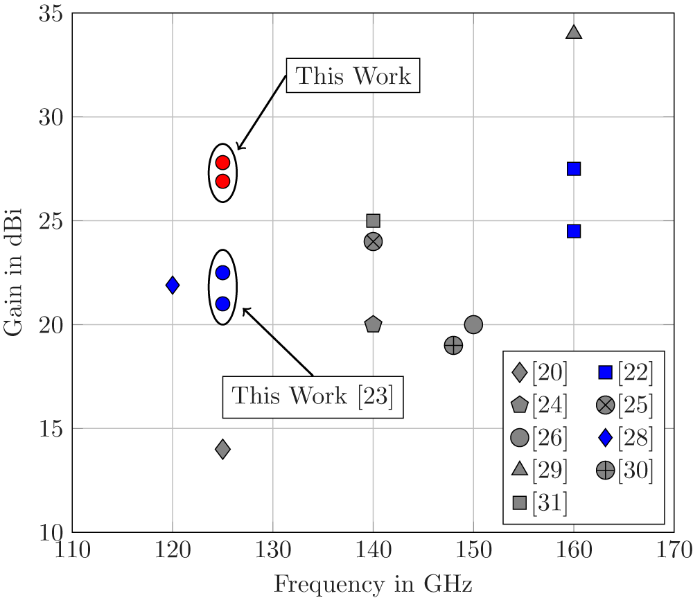
The literature survey yields that in this frequency range many different lens antennas have been designed. In order to compare the proposed lens antenna with CDWG feed with the state-of-the-art, Fig. 1 is plotted. In the plot, the targeted center frequency of the designs found in literature and their corresponding achieved gains are used as coordinates to put the markers. This includes dielectric lens antennas that are fed from the transceiver chip directly like [Reference Yoo, Kim, Keum, Son, Kim, Lee, Yang, Kim and Rieh26, Reference Manzillo, Hamani, Siligaris, Clemente and González-Jiménez30] or with conventional ones like patch antenna [Reference Bisognin, Titz, Luxey, Jacquemod, Ferrero, Lugara, Pilard, Gianesello, Gloria, Costa, Laporte, Ezzeddine, Lima and Fernandes20], slot antenna [Reference Geng, Llombart, Syed, Carluccio, Nandagopal, Alonso-delPino, Doris and Cavallo24], or waveguide/horn [Reference Chowdhury, Chakrabarti and Kumar25, Reference Derat, Schmitz, Lachner, Campo and Bruni29, Reference Gu and Bai31]. All these points are marked with grey-filled markers. The blue-filled markers represent those studies in which DWGs have been used to feed the antennas [Reference Geiger, Hitzler, Iberle and Waldschmidt22, Reference Ooms and Reynaert28]. This also includes part of this work published earlier in EuCAP’25 ([Reference Pal, Dutta and Schneider23]). The newly obtained higher gain factors of this work are marked with red-filled circles.
Comparison of the measured gain factors at their respective design frequencies for different D-band lens antennas from literature ([Reference Bisognin, Titz, Luxey, Jacquemod, Ferrero, Lugara, Pilard, Gianesello, Gloria, Costa, Laporte, Ezzeddine, Lima and Fernandes20, Reference Geiger, Hitzler, Iberle and Waldschmidt22–Reference Yoo, Kim, Keum, Son, Kim, Lee, Yang, Kim and Rieh26, Reference Ooms and Reynaert28–Reference Gu and Bai31]) where the blue and grey-filled markers represent with and without DWG feeding, respectively. The red-filled circles and the blue-filled circles ([Reference Pal, Dutta and Schneider23]) highlight the gain factors obtained in this work.
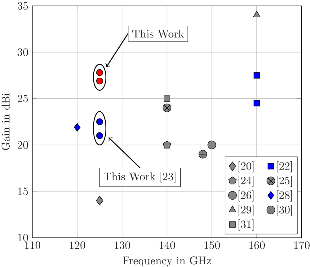
Figure 1 Long description
The graph shows a scatter plot with the x-axis labeled 'Frequency in GHz' ranging from 110 to 170 and the y-axis labeled 'Gain in dBi' ranging from 10 to 35. Various markers represent different studies of D-band lens antennas. Red-filled circles and blue-filled circles highlight gain factors from the current work and previous work, respectively. Other markers, such as diamonds, squares, pentagons, circles and triangles, represent different studies referenced by numbers in brackets. The plot visually compares the gain factors at their respective design frequencies.
Feeding of the antenna
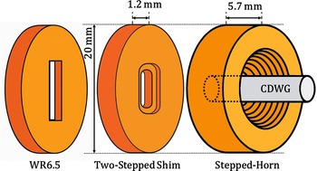
Schematic view of the transition from rectangular waveguide WR6.5 to CDWG.
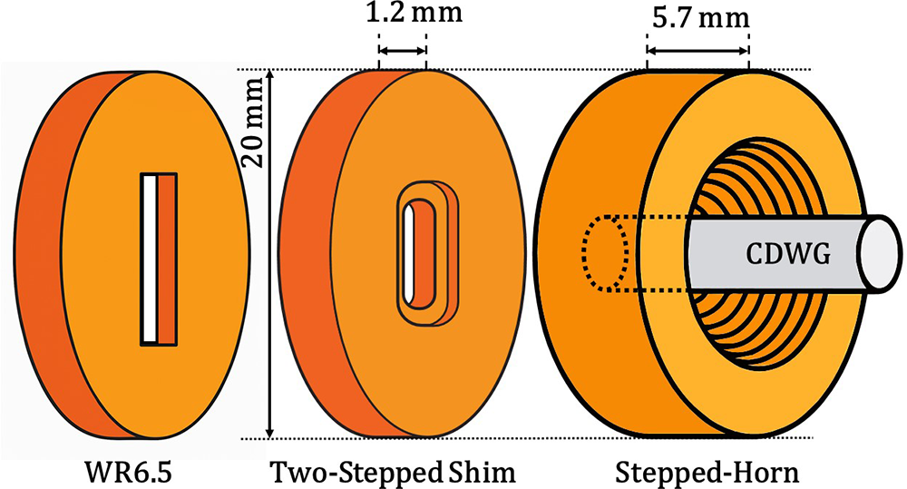
Figure 2 Long description
The diagram illustrates the transition from a WR6.5 waveguide to a CDWG. The first section labeled WR6.5 shows a rectangular waveguide. The second section, labeled Two-Stepped Shim, is depicted with a shim transition measuring 1.2 millimeters. The third section, labeled Stepped-Horn, features a multi-stepped horn with a dimension of 5.7 millimeters, leading to the CDWG. The overall structure is compact, facilitating efficient mode conversion without radiation into free space.
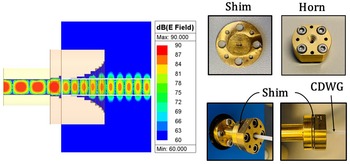
Electric field plot (magnitude) at  $125\,\mathrm{GHz}$ along the full transition structure with the DWG contour in white (left) and the fabricated prototype of the transition (right).
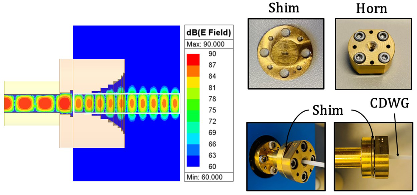
Figure 3 Long description
The left side shows an electric field plot with a color scale indicating field magnitude from 60 to 90 decibels. The plot illustrates the field distribution along a transition structure. On the right, there are three images labeled 'Shim', 'Horn' and 'CDWG'. The 'Shim' image shows a circular component with multiple holes. The 'Horn' image displays a similar circular component with screws. The 'CDWG' image shows the shim connected to a cylindrical waveguide, highlighting the assembly of these components.
The feeding of any antenna strongly regulates the overall performance. Especially with respect to a lens antenna, the feeding must be wisely designed so as to feed the lens in an efficient manner. In this case, the feed is a CDWG carrying its fundamental guided mode  $\text{HE}_{11}$. However, the standard equipment and measurement setups do usually come with a waveguide connection, in this case the standard WR6.5 with aperture dimensions $1.651\,\mathrm{mm}$ x $0.826\,\mathrm{mm}$. Therefore, a transition or mode launcher is designed to effectively convert the $\text{TE}_{10}$ (the fundamental mode of WR6.5) into the $\text{HE}_{11}$ mode of the CDWG. The transition is done by first making a two-stepped shim transition to convert the fundamental $\text{TE}_{10}$ mode of WR6.5 to the $\text{TE}_{11}$ mode of a circular metallic waveguide of the same diameter as of the CDWG and that has a dielectric filling of the same material as of the CDWG (by sticking the CDWG into the circular waveguide). Thereafter, a multi-stepped horn follows to convert the mode into the $\text{HE}_{11}$ mode of the CDWG without creating radiation into free space or exciting higher order modes into the CDWG. A schematic view of the transition structure is shown in Fig. 2. The overall transition is very compact and does not need any tapered segments (like in [Reference Geiger, Hitzler, Iberle and Waldschmidt22]). It allows one to use this as a simple “plug-n-play” device. Moreover, unlike [Reference Geiger, Hitzler, Iberle and Waldschmidt22] and [Reference Meyer, Krüger, Obermeyer and Schneider32], here the CDWG needs no alteration (like a taper or a tip) to achieve the matching. The mode launcher is designed and fabricated by the help of CNC machining on brass.
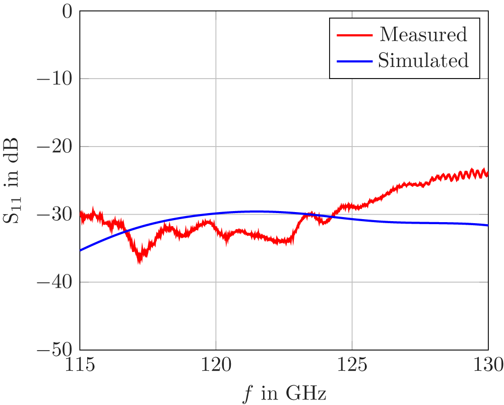
Measured and simulated reflection coefficients for the transition from WR6.5 to CDWG (LDPE,  $1.75\,\mathrm{mm}$).
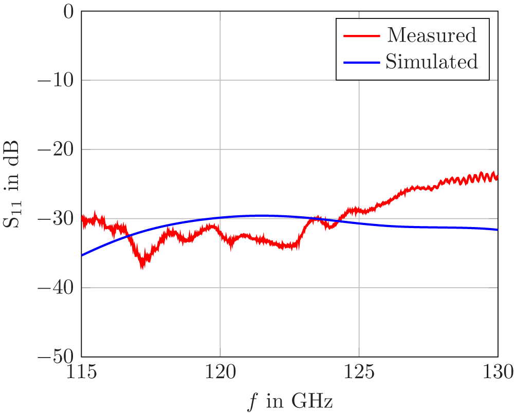
Figure 4 Long description
The graph shows reflection coefficients S subscript 11 in dB plotted against frequency f in GHz, ranging from 115 to 130. Two curves are present: a red curve labeled 'Measured' and a blue curve labeled 'Simulated'. The y-axis ranges from negative 50 to 0 dB and the x-axis ranges from 115 to 130 GHz. The measured curve fluctuates more than the simulated curve, which is smoother. The measured curve starts below negative 30 dB and rises towards negative 20 dB, while the simulated curve remains relatively stable around negative 30 dB.
In this work, the CDWG that is used is a solid core  $1.75\,\mathrm{mm}$ diameter waveguide made up of low-density polyethylene (LDPE) that has the relative permittivity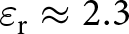 $\varepsilon_\text{r}\approx2.3$ and a loss tangent of approx.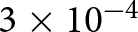 $3\times10^{-4}$ at this frequency range [Reference Afsar33]. The magnitude of the electric field along the transition and the pictures of the fabricated prototypes are shown in Fig. 3. Several back-to-back measurements are taken in VNA to quantify the return loss and the insertion loss of the transitions. The reflection coefficients ( $\text{S}_{\text{11}}$) of the transition are measured at one port by terminating the CDWG with absorber. They are presented in Fig. 4, where the “ $\text{S}_{\text{11}}$ in dB” denotes the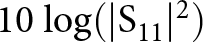 $10\ \mathrm{log} ({|\text{S}_{\text{11}}}|^2)$ which is equal to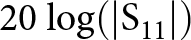 $20 \ \mathrm{log} ({|\text{S}_{\text{11}}}|)$. The same applies to all the other S-parameter plots shown later in this work. It shows that the transition has a return loss of better than $25\,\mathrm{dB}$. The back-to-back measurements with different lengths of the waveguide concluded the insertion loss of per transition to be in between $0.2-0.3\,\mathrm{dB}$ and the attenuation of the CDWG to be in between $2.5-3.5\,\mathrm{dB}/\mathrm{m}$ in the desired frequency range [Reference Schneider and Meyer16]. In [Reference Schneider and Meyer16], efficient design charts are presented that can be used to design such optimal CDWGs as per need.
Design of the lens antenna
After the CDWG is chosen for the feeding, the lens antenna design has to be made. The lens antenna can typically have different shapes like spherical, elliptical, hemispherical, etc. An extension (like a cylinder) with a flat base is often added to these shapes. This could provide better phase uniformity, improved matching, and also an easier feed integration. To design an efficient antenna, first, the key parameters are identified, and then a lens contour (including the extension) is derived using optical rays and electrical phase relationships. After that, with the help of full-wave EM simulations in Ansys High Frequency Structure Simulator (HFSS), a detailed analysis is conducted to study the different contours with respect to their matching and gain performances. The next sections illustrate this study and present the findings.
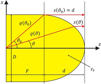
Dielectric lens (relative permittivity  $\varepsilon_\text{r}$) with extension showing two different rays at angles $\vartheta$ and $\vartheta_0$ generating a plane wavefront.
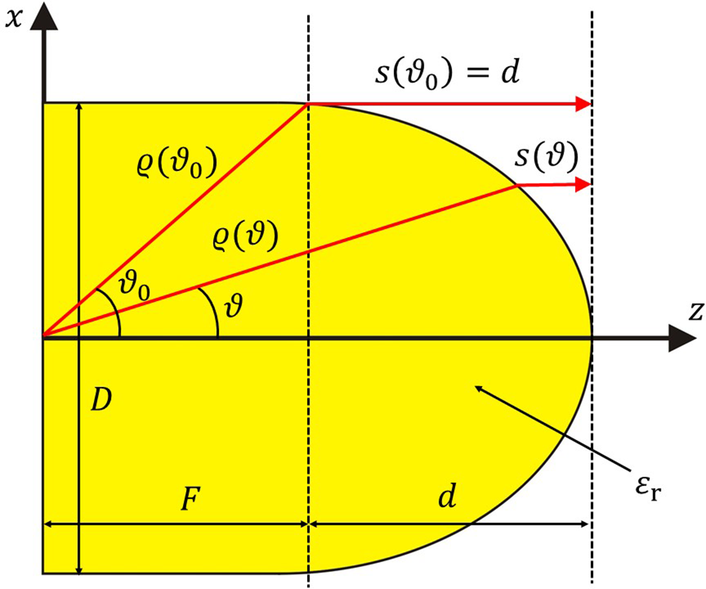
Figure 5 Long description
The diagram illustrates a dielectric lens with two rays at angles theta and theta subscript 0. The rays originate from a point on the lens and extend outward, forming a plane wavefront. The lens is labeled with dimensions D for diameter, F for extension height and d for depth. The relative permittivity is denoted by epsilon subscript r. The rays are shown with paths rho left parenthesis theta subscript 0 right parenthesis and rho left parenthesis theta right parenthesis, with corresponding phase delays s left parenthesis theta subscript 0 right parenthesis equals d and s left parenthesis theta right parenthesis. The x and z axes are marked, indicating the orientation of the lens and rays.
Derivation of the lens contour
In order to derive the contour of the lens, the laws of geometrical optics and the phase delay relations are exploited. Fermat’s law is utilized, and it is ensured that all rays generated from the considered feeding point that move toward the contour of the lens have the equal electrical lengths. This means all rays independent of the angle reach the outer most reference plane with the same time delay and thereby form a plane wavefront in front of the lens. This technique is well described in textbooks, for example, in [Reference Balanis34] where it is used to derive the contour of a parabolic reflector antenna. The same concepts are also used to design dielectric lenses in [Reference Zaidi, Ali, Abd Hamid, Abd Rahman and Tengah35] and [Reference Yue, Guo, Li and Guo36]. To achieve this plane wavefront, the feed has to be at the lens’s focal point. Figure 5 shows two different rays originating from the feed placed at the focal point, generating the plane wavefront in front of the lens. The refractive index is 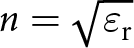 $n=\sqrt{\varepsilon_\text{r}}$, $F$ denotes the lens extension height (not the focal distance), $d$ is the depth, and $D$ is the diameter of the lens. Any generic ray $\varrho(\vartheta)$ that makes an angle $\vartheta$ with the $z-$axis must face the same phase delay, as the ray that is along the $z-$axis ( $\vartheta=0$) would face. This can be given mathematically in an equation by:
 \begin{equation}
n \varrho(\vartheta) + s(\vartheta) = n(F + d)
\end{equation}
\begin{equation}
n \varrho(\vartheta) + s(\vartheta) = n(F + d)
\end{equation}Also, from Fig. 5 geometrically, it can be seen that:
 \begin{equation}
\varrho(\vartheta) \cos(\vartheta) + s(\vartheta) = F + d
\end{equation}
\begin{equation}
\varrho(\vartheta) \cos(\vartheta) + s(\vartheta) = F + d
\end{equation} On combining both of them and simplifying the generic  $\varrho(\vartheta)$ for an angle $\vartheta$ can be summarized as:
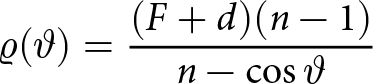 \begin{equation}
\varrho(\vartheta) = \frac{(F + d)(n - 1)}{n - \cos \vartheta}
\end{equation}
\begin{equation}
\varrho(\vartheta) = \frac{(F + d)(n - 1)}{n - \cos \vartheta}
\end{equation} Also, for the outermost ray  $\varrho(\vartheta_0)$, making an angle $\vartheta_0$, i.e., the maximum angular stretch for illuminating the lens (as can be seen in Fig. 5), it can be geometrically written that,
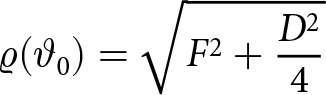 \begin{equation}
\varrho(\vartheta_0) = \sqrt{F^2 + \frac{D^2}{4}}
\end{equation}
\begin{equation}
\varrho(\vartheta_0) = \sqrt{F^2 + \frac{D^2}{4}}
\end{equation}and from phase delay perspective, it can be written as,
 \begin{equation}
n\varrho(\vartheta_0) + d = n(F+d).
\end{equation}
\begin{equation}
n\varrho(\vartheta_0) + d = n(F+d).
\end{equation} Making use of the above equations, the depth  $d$ is found out as:
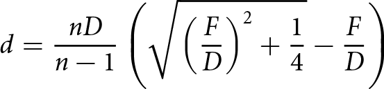 \begin{equation}
d = \frac{n D}{n - 1} \left( \sqrt{\left({\frac{F}{D}}\right)^2 + \frac{1}{4}} - \frac{F}{D} \right)
\end{equation}
\begin{equation}
d = \frac{n D}{n - 1} \left( \sqrt{\left({\frac{F}{D}}\right)^2 + \frac{1}{4}} - \frac{F}{D} \right)
\end{equation} Finally, after putting it all together, the contour of the locus of the lens, i.e., the  $x$ and $z$ coordinates can be given for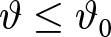 $\vartheta \le \vartheta_0$ as:
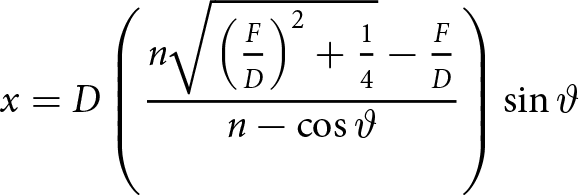 \begin{equation}
x = D \left(\frac{n \sqrt{\left({\frac{F}{D}}\right)^2 + \frac{1}{4}} - \frac{F}{D}}{n - \cos \vartheta} \right) \sin \vartheta
\end{equation}
\begin{equation}
x = D \left(\frac{n \sqrt{\left({\frac{F}{D}}\right)^2 + \frac{1}{4}} - \frac{F}{D}}{n - \cos \vartheta} \right) \sin \vartheta
\end{equation}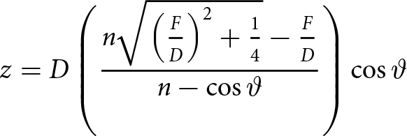 \begin{equation}
z = D \left(\frac{n \sqrt{\left({\frac{F}{D}}\right)^2 + \frac{1}{4}} - \frac{F}{D}}{n - \cos \vartheta} \right) \cos \vartheta
\end{equation}
\begin{equation}
z = D \left(\frac{n \sqrt{\left({\frac{F}{D}}\right)^2 + \frac{1}{4}} - \frac{F}{D}}{n - \cos \vartheta} \right) \cos \vartheta
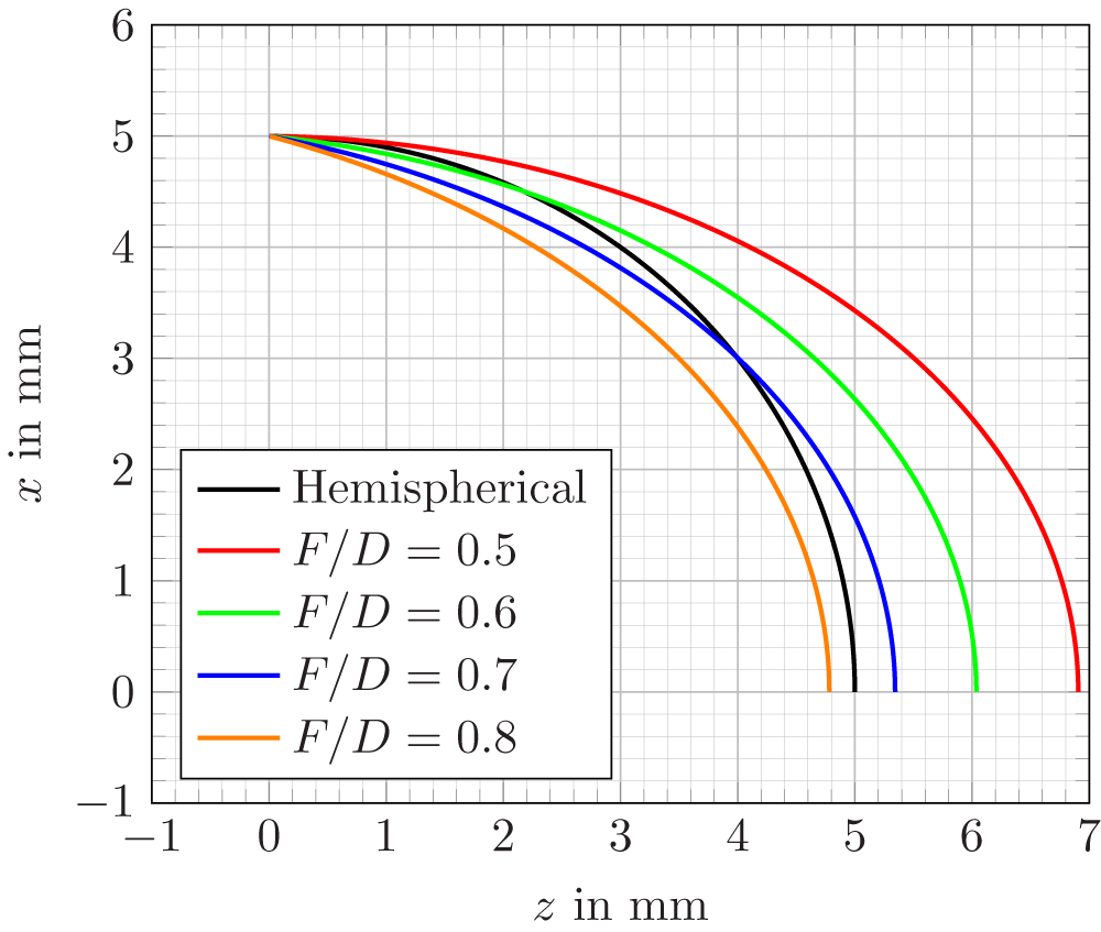
\end{equation}Derived elliptical contours of the lens for diameter  $D=10\,\mathrm{mm}$ with different $F/D$ ratios and a hemispherical contour of the same diameter (lens material: PTFE).
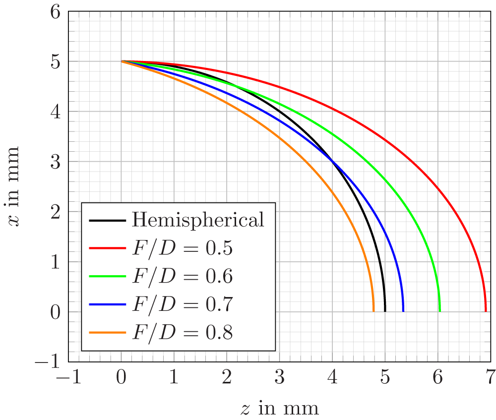
Figure 6 Long description
The x-axis is labeled 'z in mm' and the y-axis is labeled 'x in mm'. The plotted lines represent different F over D ratios: 0.5, 0.6, 0.7 and 0.8, along with a hemispherical contour. The contours are plotted with respect to the x and z coordinates, showing how the shape changes with varying F over D ratios.
For a diameter of  $D=10\,\mathrm{mm}$,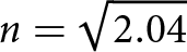 $n=\sqrt{2.04}$ (made of PTFE with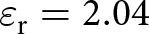 $\varepsilon_\text{r}=2.04$) and multiple values of $F/D$ ratios, the derived contours are plotted in Fig. 6 with respect to the $x$ and $z$ coordinates (excluding the extension and the lower half of the lens). It can be seen that the derived contour appears to be an elliptical segment. As the $F/D$ ratio increases, the depth of the lens decrease consequently making the elliptical contour more close to an spherical arc. For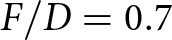 $F/D=0.7$, the elliptical contour is closer to a perfect hemisphere.
The analytical approach to find the contour of the lens is quite simple and good for an initial indication of the contour shape. It is, however, important to note that the approach assumes that the feeding point of the lens antenna is also the phase center of the lens. In reality, it might differ especially at different frequencies. In that case, one can utilize more complex field analysis techniques and algorithms like Geometrical Optics/Physical Optics (GO/PO), etc., to solve for the contour. Having said that, the simple ray-based approach proposed here and the similar approaches used in [Reference Geiger, Hitzler, Iberle and Waldschmidt22] and [Reference Pohl and Gerding37], also give a valid basic idea of the contour, which can be further optimized and analyzed using full-wave EM simulations.
Simulative analysis
It can be seen from the contour derivation that an elliptical contour could enable all rays to reach the outer surface of the lens with the same time delay and thereby a plane wavefront could be radiated from the front of the lens. However, an elliptical lens antenna could also suffer from greater mismatch because the rays that are reflected from the outer surface of the lens, come back to the same focal point where the feeding is [Reference Neto, Maci and de Maagt38]. Therefore, it needs to be verified via wave simulations how these lenses perform quantitatively. It is imperative to compare the derived contour with other contour shapes like hemispherical or a spherical arc in terms of the gain and matching. Additionally, for an efficient design, it is important to study and analyze the influence of the key structural parameters 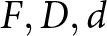 $F, D, d$ and also the material ( $\varepsilon_\text{r}$). Typically, for lens antenna designs, it is more common to work with the ratios of these structural dimensions to allow direct implementations at different frequencies. Therefore, in the later sections, the performance of the antenna with respect to matching and gain is studied through a detailed simulative analysis for different $F/D$ and $d/D$ ratios.
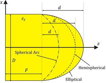
Dielectric lens showing the different contours where solid is elliptical (derived contour), dashed represents the hemispherical (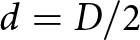 $d=D/2$), and dash-dotted represents the lens with a spherical arc (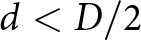 $d \lt D/2$).
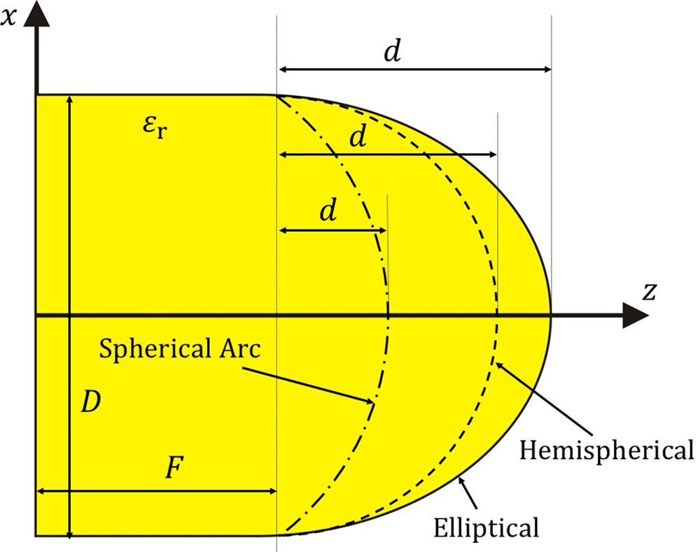
Figure 7 Long description
The diagram illustrates different contours of a dielectric lens, including elliptical, hemispherical and spherical arc shapes. The elliptical contour is represented by a solid line, the hemispherical contour by a dashed line and the spherical arc by a dash-dotted line. The dimensions are labeled with 'd' for depth, 'D' for diameter and 'F' for lens height. The relative permittivity is denoted by 'epsilon subscript r'. The axes are labeled 'x' and 'z'.
Comparison of different contours
Upon carefully observing Fig. 6, it can be noticed that if the lens height  $F$ is made larger, it reduces the needed depth $d$, making the contour more comparable to a spherical arc segment (in 2D). To investigate further, different contours are modeled, and full-wave simulations are carried out in HFSS. First, a comparison is made between a hemispherical (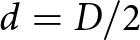 $d=D/2$) and an elliptical lens (with contour derived in section “Derivation of the lens contour”). Both the lenses are made up of High Density Polyethylene (HDPE) which typically has a relative permittivity similar to LDPE that is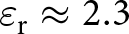 $\varepsilon_\text{r} \approx 2.3$. For both the cases, the $1.75\,\mathrm{mm}$ diameter LDPE CDWG is attached to the lens antennas. This is done to avoid additional reflections from material mismatch as both have similar permittivity values. It has also been verified through simulations that even if there is a small difference in the $\varepsilon_\text{r}$ between LDPE and HDPE (typically in the range of $\pm$0.05), this has a negligible influence on the matching of the antenna CDWG combination. Therefore, for all simulations the $\varepsilon_\text{r}$ for LDPE and HDPE are kept equal to 2.3. The required $\text{HE}_{11}$ mode is excited using a wave-port in simulations. Figure 7 shows the two-dimensional contours of the different lenses, i.e., elliptical, pure hemispherical (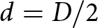 $d=D/2$), and also with a spherical arc (where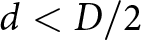 $d \lt D/2$).
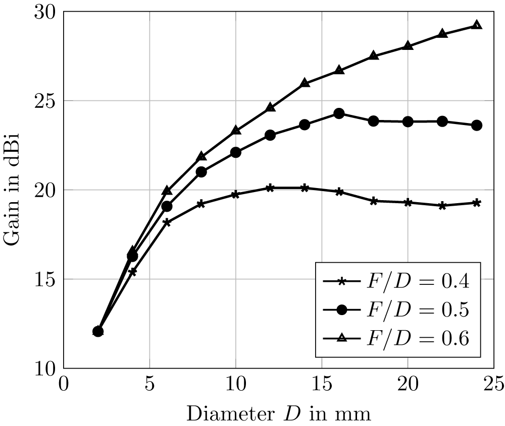
Simulated peak gains at  $125\,\mathrm{GHz}$ for hemispherical contour-based HDPE lens for different $F/D$ ratios over different values of diameter $D$.
$D$.
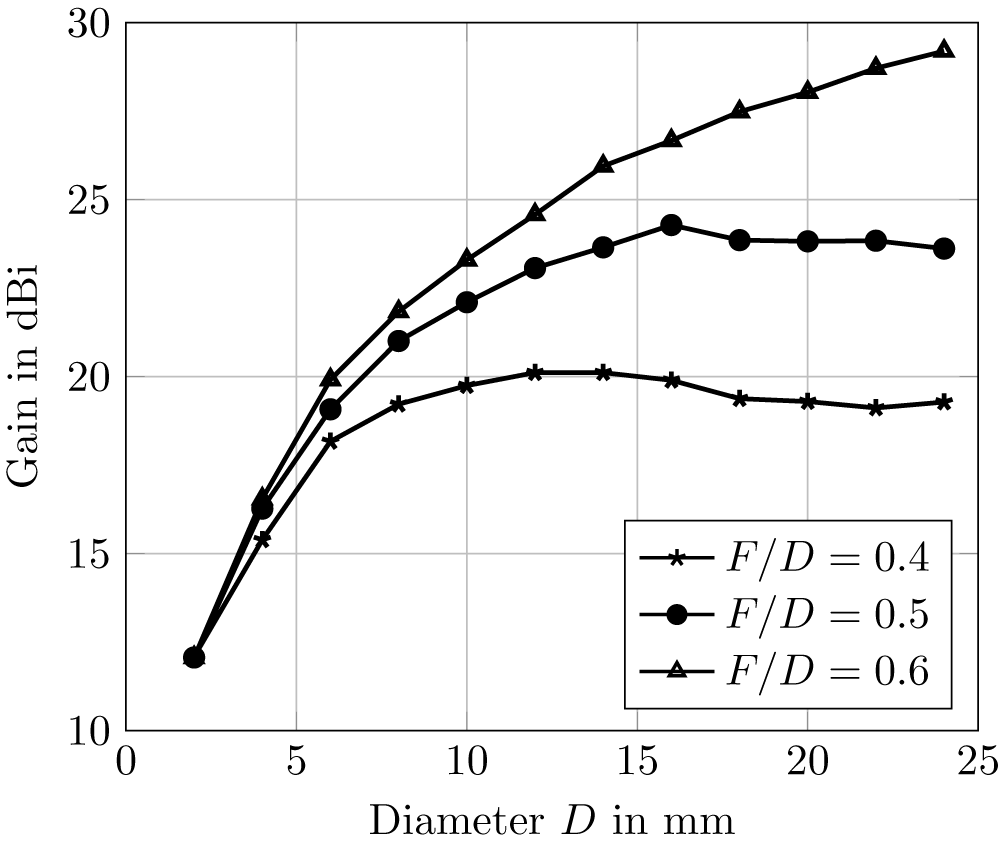
Figure 8 Long description
A line graph showing the relationship between gain in dBi and diameter D in millimeters. The x-axis is labeled 'Diameter D in mm' and the y-axis is labeled 'Gain in dBi'. Three curves represent different F over D ratios: 0.4, 0.5 and 0.6. The curve for F over D equals 0.4 starts at approximately 12 dBi and increases to about 18 dBi, then levels off. The curve for F over D equals 0.5 begins at around 15 dBi, rises to about 22 dBi and then stabilizes. The curve for F over D equals 0.6 starts at approximately 17 dBi, increases steadily, reaching around 28 dBi at the largest diameter. The graph indicates that as the diameter increases, the gain also increases, with different saturation points for each F over D ratio.
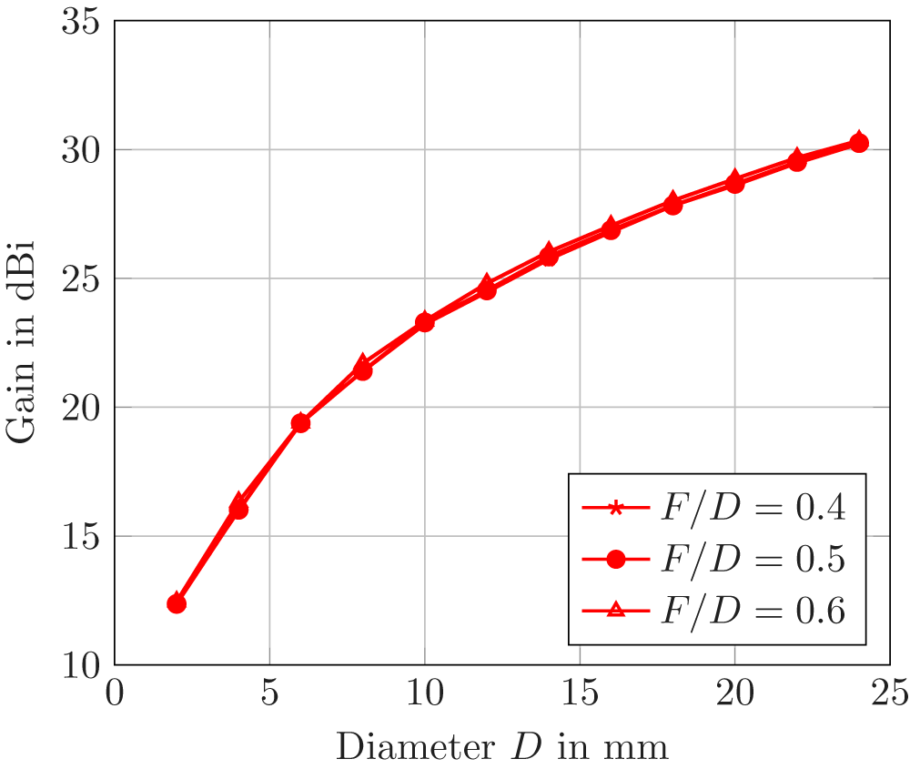
Simulated peak gains at  $125\,\mathrm{GHz}$ for elliptical contour-based HDPE lens for different $F/D$ ratios over different values of diameter $D$.
$D$.
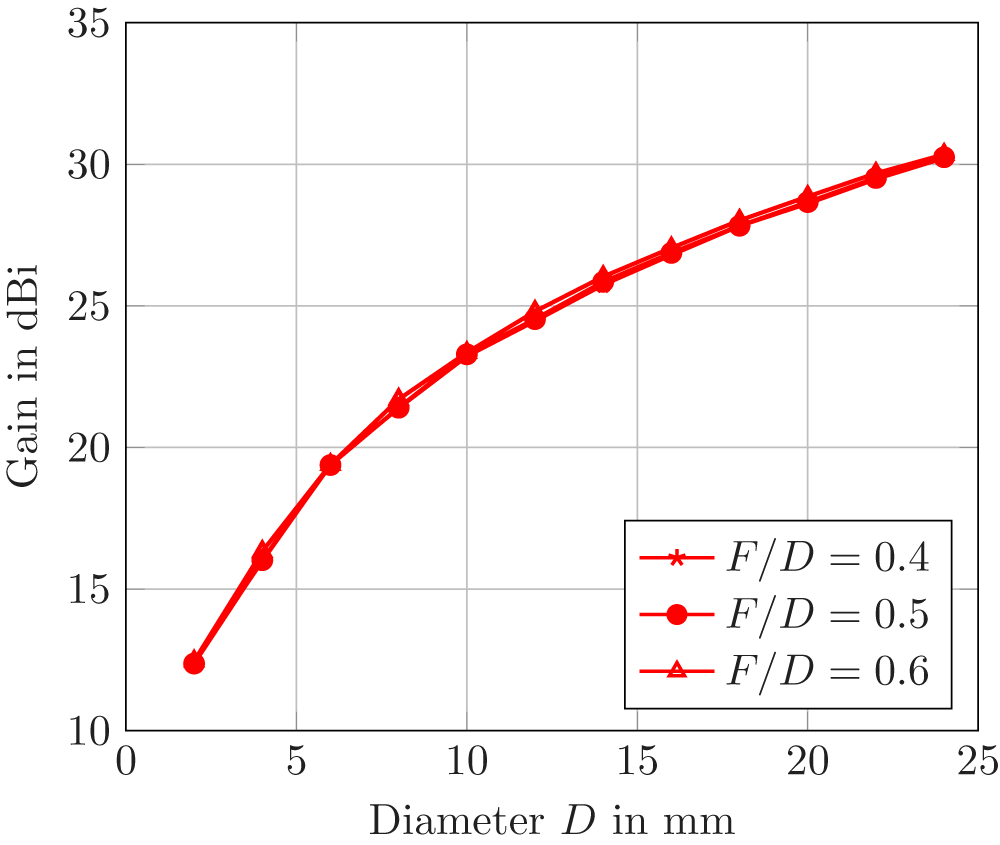
Figure 9 Long description
The graph shows gain in dBi on the y-axis and diameter D in millimeters on the x-axis. Three curves represent different F over D ratios: 0.4, 0.5 and 0.6. The gain increases with diameter, starting from around 10 dBi at 0 millimeters and reaching approximately 30 dBi at 25 millimeters. The curves for F over D ratios 0.4, 0.5 and 0.6 are closely aligned, indicating similar gain trends across these ratios. The legend identifies each curve with different symbols: a star for 0.4, a circle for 0.5 and a triangle for 0.6.
Now, to investigate the performance of these shapes, the effects of different parameters are studied. It is obvious that the physical dimensions strongly determine the lens’ performance like when one takes a lens with larger diameter it is also expected to provide a higher gain up to a certain extent after which it saturates. This is validated via simulations whose results are presented in Figs. 8 and 9 for hemispherical and elliptical contours, respectively. Here, the peak simulated gain at  $125\,\mathrm{GHz}$ is plotted against the diameter of the lens for different $F/D$ ratios for hemispherical HDPE lens (Fig. 8) and an elliptical HDPE lens (Fig. 9). From the plots of both lens contours it can be verified that as the diameter increases, the gain values increase with $D$ and then saturates (see $F/D$ ratios of $0.4$ and $0.6$ for hemispherical). This is also analogous to the study shown in [Reference Konstantinidis, Feresidis, Constantinou, Hoare, Gashinova, Lancaster and Gardner39] where the gain is plotted against different $F/D$ ratios for different $D$ values. However, the interesting point to be observed is that in case of the elliptical lens, for all $F/D$ ratios the plots almost overlap, i.e., same gain factors are obtained in simulations at a certain diameter $D$ almost independent of the $F/D$ ratio. However, this is not true for the case of hemispherical lens. In that case, to achieve a higher gain an increased extension $F$ is also needed with an increasing $D$. Overall, it can be concluded that the simulated gain of the elliptical lens is prominently higher than the hemispherical shape (for lower $F/D$ ratios). This is expected because the elliptical contour was found from the derivations. For example, for $D=10\,\mathrm{mm}$ and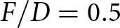 $F/D=0.5$, the simulated gain for the hemispherical lens is $\approx1\,\mathrm{dB}$ lower than the elliptical one. It is noteworthy that the contour does effect the matching of the antenna too. Therefore, it is imperative to compare the return loss as well. A lens contour that achieves the highest gain factor need not necessarily mean that it also has the best matching.
Trade-off between gain and matching
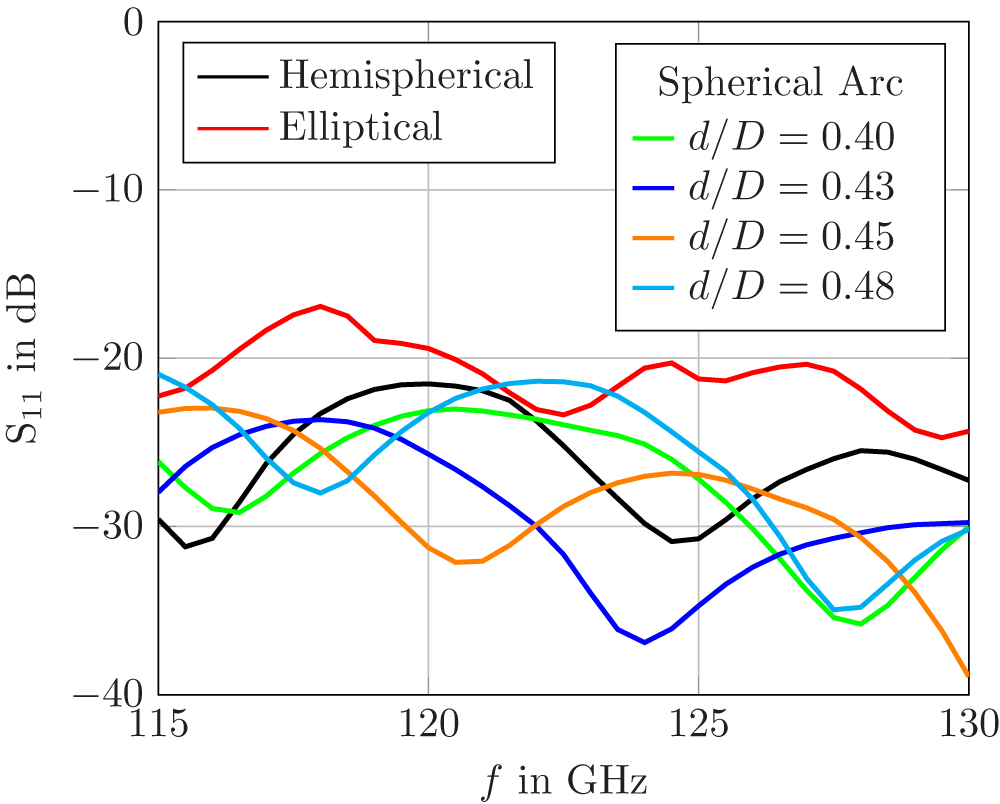
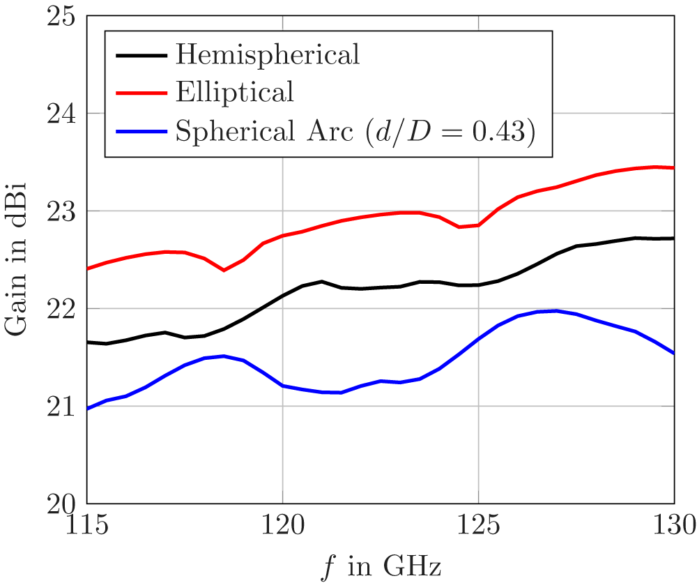
In order to validate the previous assumption, the simulative analysis is done with respect to the matching as well. The simulated reflection coefficients ( $\text{S}_{11}$) of the hemispherical and elliptical contours are plotted in Fig. 10 for a lens made of HDPE with $D=10\,\mathrm{mm}$ and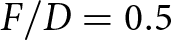 $F/D=0.5$. It can be seen that the hemispherical contour has a better matching as compared to the elliptical one. The match is further improved when the depth $d$ is reduced, i.e., by making it a spherical arc. Figure 10 also shows the simulated reflection coefficients of this spherical arc lens with different $d/D$ ratios. It can be seen that for a $d/D$ ratio of $0.43$ the best matching among the others is observed in simulations. However, from the previous section, it is also clear that the gain is higher for the elliptical case although it is the comparison of the peak gain at only one frequency. It is needed to compare the gain factors over the entire frequency range as well. So, the simulated gain factors of the spherical arc with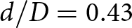 $d/D=0.43$, the elliptical, and the hemispherical lens for the entire frequency range are plotted in Fig. 11. There, it can be seen that the gain for the spherical arc lens is a bit lower than the other lenses, however, a better match is obtained for the same (without altering the CDWG). Therefore, this opens up for a possible trade-off between the gain and matching performance, and one can make an intelligent choice of the contour based on one’s requirement.
Simulated reflection coefficients  $\text{S}_{11}$ over frequency for HDPE lenses with $D=10\,\mathrm{mm}$ and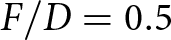 $F/D=0.5$ and different contours.
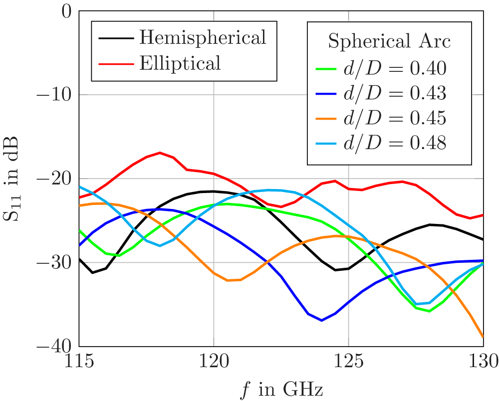
Figure 10 Long description
The graph shows simulated reflection coefficients, labeled as S subscript 11 in decibels, plotted against frequency, labeled as f in gigahertz. It includes curves for hemispherical and elliptical lenses, as well as spherical arc lenses with different d over D ratios: 0.40, 0.43, 0.45 and 0.48. The hemispherical lens is represented by a black curve, the elliptical lens by a red curve and the spherical arc lenses by green, blue, orange and light blue curves corresponding to the respective d over D ratios. The frequency range is from 115 to 130 gigahertz and the reflection coefficient values range from negative 40 to 0 decibels.
Simulated gain over frequency for HDPE lenses with  $D=10\,\mathrm{mm}$ and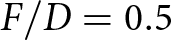 $F/D=0.5$ and different contours.
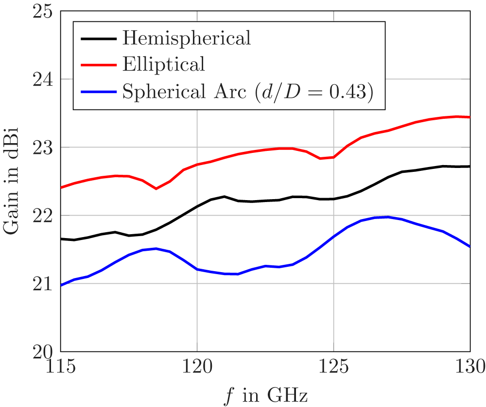
Figure 11 Long description
A line graph showing the gain in dBi for three different lens contours: hemispherical, elliptical and spherical arc with d over D equals 0.43. The x-axis is labeled 'f in GHz' and ranges from 115 to 130 GHz. The y-axis is labeled 'Gain in dBi' and ranges from 20 to 25. The hemispherical lens is represented by a black line, the elliptical lens by a red line and the spherical arc lens by a blue line. The elliptical lens shows the highest gain, followed by the hemispherical and spherical arc lenses.
Inserting the CDWG into the lens
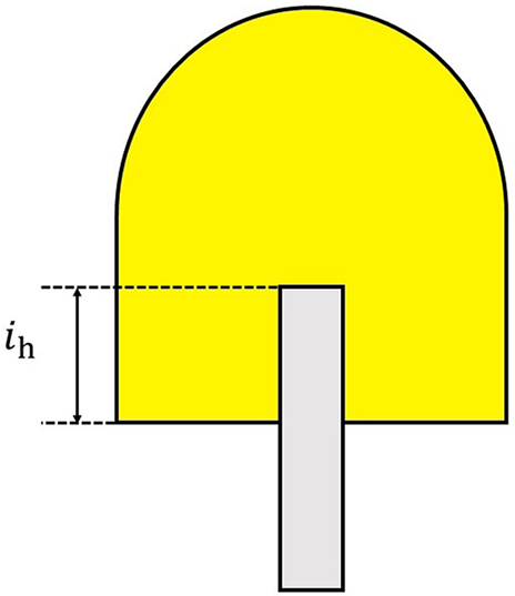
Simple sketch showing the CDWG inserted into the lens up to a depth of  $i_\text{h}$.
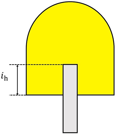
Figure 12 Long description
The diagram illustrates a cylindrical object inserted into a dome-shaped structure. The dome is positioned above the cylinder, which is partially inserted into it. The depth of insertion is marked with a label i subscript h, indicating the measurement from the top of the cylinder to the point where it enters the dome. The dome has a rounded top and flat bottom, while the cylinder is vertically oriented beneath it.
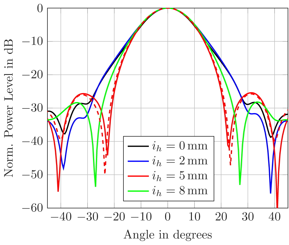
Simulated normalized E-plane ( $-$) radiation patterns for a PTFE lens at $125\,\mathrm{GHz}$ for $D=10\,\mathrm{mm}$,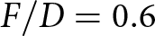 $F/D=0.6$ and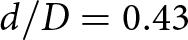 $d/D=0.43$ with a spherical arc contour for different insertion depths of the CDWG. Simulated H-plane ( $--$) radiation pattern for insertion depth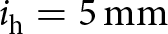 $i_\text{h}=5\,\mathrm{mm}$.
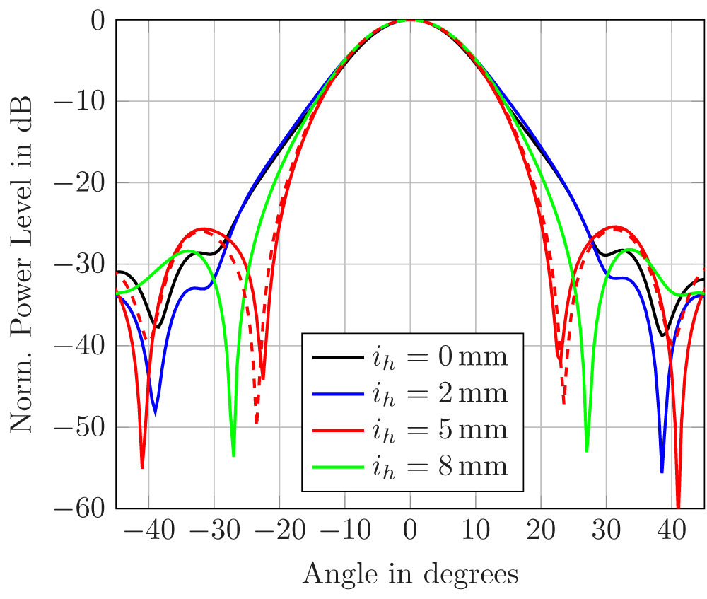
Figure 13 Long description
The graph shows normalized power level in decibels on the y-axis and angle in degrees on the x-axis. Four curves represent different insertion depths: black for 0 millimeters, blue for 2 millimeters, red for 5 millimeters and green for 8 millimeters. Each curve displays variations in power level across angles from negative 40 to positive 40 degrees. The red curve includes both solid and dashed lines, indicating additional data points or variations. The graph illustrates how power levels change with different insertion depths, showing peaks and troughs at various angles.
Simulated 3D-radiation patterns along with the picture of the models for PTFE-II-E (left) and PTFE-III-E (right) lens antennas at  $125\,\mathrm{GHz}$. The color legends show the gain factors in $\mathrm{dB}$.
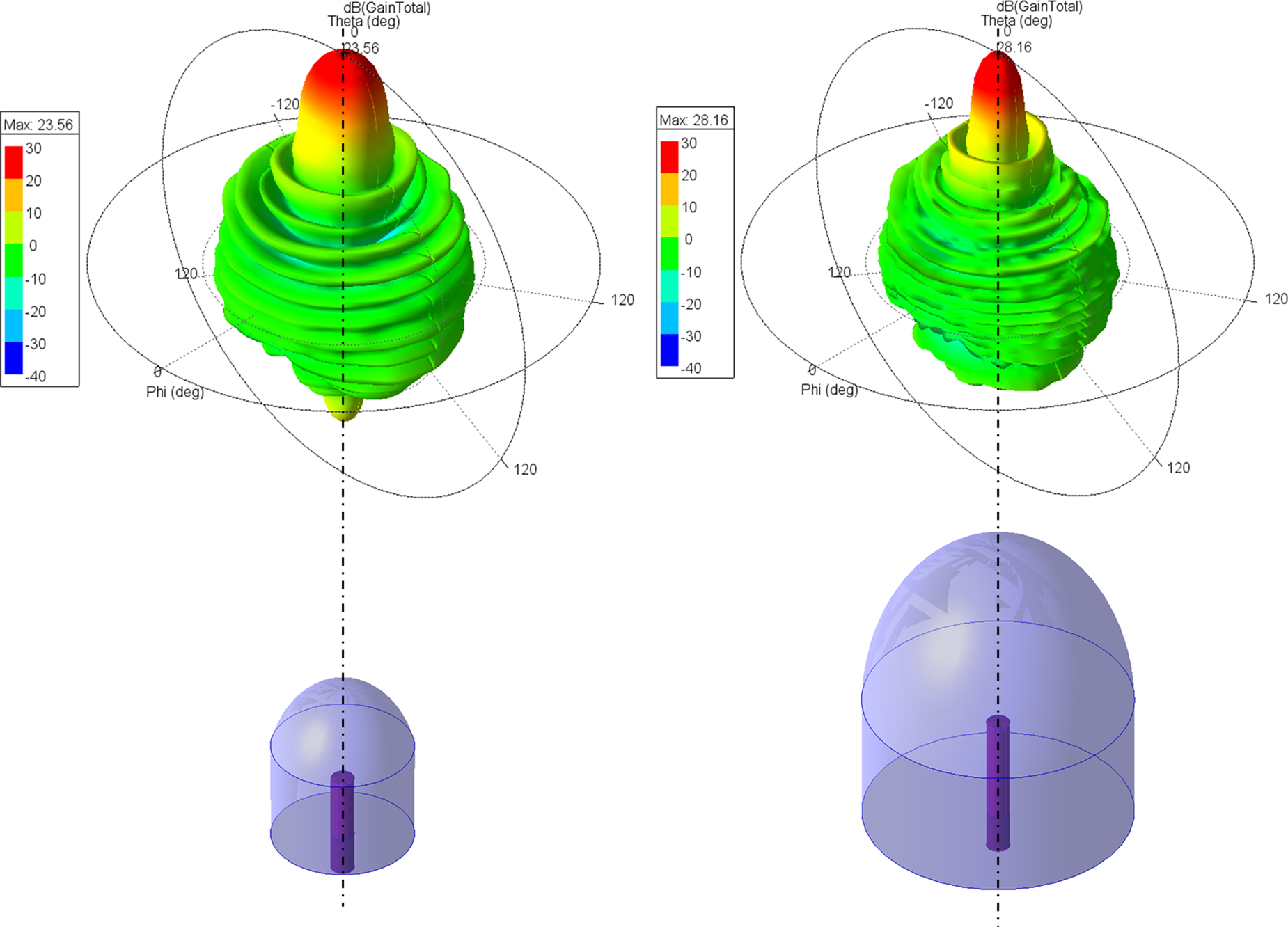
Figure 14 Long description
The image shows two simulated 3D radiation patterns for PTFE-II-E and PTFE-III-E lens antennas. The left pattern represents the PTFE-II-E lens, while the right pattern represents the PTFE-III-E lens. Both patterns illustrate the gain factors in decibels, with a color gradient indicating different levels of gain. The patterns are depicted above models of the lens antennas, which are shown as transparent structures with a central component. The radiation patterns are more narrow for the larger diameter lens, indicating greater gain. The patterns include lines representing the E and H-plane, which are quite identical for both lenses.
Till now, for all the analysis, it was assumed that the circular aperture surface of the CDWG makes a perfect flat contact with the larger circular surface of the lens. This of course brings some mechanical challenges and demands for an adapter or holding structure to keep everything in place. This can be mitigated by simply inserting the DWG into the lens. This idea of inserting the CDWG to feed the antenna would make the overall system even more compact, and the lens antennas would then enable a simpler “plug-n-play” mounting as shown by the schematic diagram depicted in Fig. 12. However, this could also impact the overall performance of the lens antenna if lens’ material and CDWG material are different. Therefore, the effect of inserting the CDWG on the matching (if the CDWG and lens are of different material), the gain, and the radiation patterns are verified through simulations. Since one can see such an effect only when the CDWG material and the lens material are different, a spherical arc lens made of PTFE (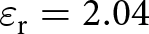 $\varepsilon_\text{r}=2.04$) with $D=10\,\mathrm{mm}$,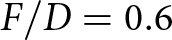 $F/D=0.6$ and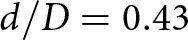 $d/D=0.43$ is taken for the analysis. At the center of the lens a hole is made where the LDPE (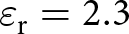 $\varepsilon_\text{r}=2.3$) CDWG is inserted. The depth of the insertion $i_\text{h}$ is varied and the behavior with respect to the performance is analyzed. From simulations, it is observed that inserting the CDWG into the lens does not have a significant effect on the matching. A max. change of $1-2\,\mathrm{dB}$ is observed with all values still lying below $-25\,\mathrm{dB}$ for all $i_\text{h}$ values. Therefore, it is not detailed here. However, an interesting observation is found in the radiation pattern of the antenna, which is plotted in Fig. 13. With the insertion of the CDWG, the main beam becomes more prominent. For example, for the case when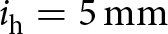 $i_\text{h}=5\,\mathrm{mm}$ it can be seen that the first null points are sharply visible unlike the case where the CDWG is just placed in contact to the lens but not inserted at all ( $i_\text{h}=0$). This happens plausibly because the concentration of the fields now taper into the waveguide therefore reducing spilling of the fields onto the sides. Important to note that here this is only shown for the center frequency point. The phenomenon is observed across the entire frequency range and upon further analysis with other models it is concluded that the insertion of the CDWG into the lens antenna helps to not only make the system more compact but could also provide a more sharp main beam. In certain cases, this could be leveraged to reduce the side lobe levels. But all this could harm the peak gain value slightly.
In order to depict the overall radiation pattern in a 3D view, the simulated beam patterns at  $125\,\mathrm{GHz}$ are plotted in Fig. 14 for PTFE-II-E and PTFE-III-E lenses along with a picture of the simulation model. It can be seen that for the larger diameter lens, the beam is more narrow as compared to smaller lens which thereby also gives a greater gain. Interestingly, it is also observed that the radiation patterns in the E and H planes are quite identical. This can also be seen in Fig. 13, where the simulated E and H-plane patterns are plotted in solid and dashed lines, respectively, for an exemplary insertion depth of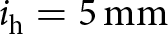 $i_\text{h} = 5\,\mathrm{mm}$. This is an advantage of using this lens structure over standard rectangular horn antennas where the E and H-plane patterns differ significantly, even if, the height and width of the horn are the same. The overall simulation results with respect to matching, gain as well as the field radiations are analyzed in depth for not only the center frequency but also for the entire targeted bandwidth of $115-130\,\mathrm{GHz}$. The lens antenna setup shows good simulative performance (RL $ \gt 25\,\mathrm{dB}$, gain $ \gt 20\,\mathrm{dB}$) in the entire $15\,\mathrm{GHz}$ bandwidth (12% fractional bandwidth). Some mechanical issues, for example, the proper contact between the CDWG and the lens, the proper insertion of the CDWG or the fabrication quality in general could still limit the performance.
E-field magnitude at  $125\,\mathrm{GHz}$ for lens antenna prototypes PTFE-I, PTFE-II-E, and PTFE-II-S showing the lens outline in white and the CDWG outline in black.
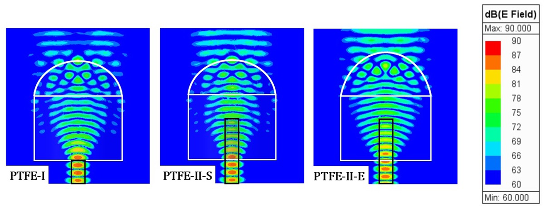
Figure 15 Long description
Three images display the electric field magnitude for different lens antenna prototypes labeled PTFE-I, PTFE-II-S and PTFE-II-E. Each image shows a lens outline in white and a CDWG outline in black. The electric field distribution is represented with varying colors, corresponding to dB values ranging from 60 to 90, as indicated by the color scale on the right. The scale includes colors from blue to red, with blue representing lower values and red representing higher values. The images illustrate the differences in field distribution across the three prototypes.
Final prototypes
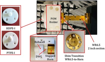
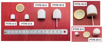
After the various simulations and detailed analysis of the results with respect to the effect of different parameters and contours, the next step is to decide upon the final design for fabrication and experimental validations. The final choice is efficiently done considering some comparison strategies. First, to validate the performance of the spherical arc lens, two different lenses, one with HDPE and another with PTFE (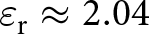 $\varepsilon_\text{r}\approx2.04$) are decided. The final dimensions of all the fabricated lenses are given in Table 1. The two lens antennas are fixed with a holding structure made of Polyoxymethylene (POM) (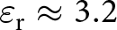 $\varepsilon_\text{r}\approx3.2$) with Rohacell (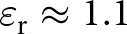 $\varepsilon_\text{r}\approx1.1$) structure inside. A flange is also made together with the lens antenna structure, which is then screwed with the holder so that the CDWG feed can be kept in good contact with the lens. This can be seen in Fig 16. Henceforth, these two lenses are termed as HDPE-I and PTFE-I. They are also shown in Fig. 16. Additionally, to make the setup more compact and discard the holding structure, another PTFE lens is made where the flange and holder are taken out, and the CDWG is inserted into the lens by making a $5\,\mathrm{mm}$ deep hole at the center. This is termed as PTFE-II-S (S-Spherical). Now, to compare the contours especially the arc one with the derived elliptical contour, a lens of the same diameter is manufactured. In this also, the CDWG is inserted $5\,\mathrm{mm}$ deep inside the lens. This is termed as PTFE-II-E (E-Elliptical). Its final dimensions are given in Table 1. In some applications, to meet the link budget, often higher gain is required. To have some antennas with such high gain values and also to validate the fact that the increased diameter also increases the gain factor, two large antennas of diameter $D=20\,\mathrm{mm}$ are manufactured. For them also, the same PTFE material is used and both the elliptical contour and spherical arc contours are manufactured. They are termed as PTFE-III-E and PTFE-III-S, and their final dimensions are also given in Table 1. The manufactured PTFE-II and PTFE-III prototypes are shown in Fig. 17. All the prototypes are manufactured via CNC milling. The magnitude of the electric fields is also plotted in Fig. 15 to show the difference between the different lenses.
HDPE-I and PTFE-I prototypes along with the POM holder and transition.
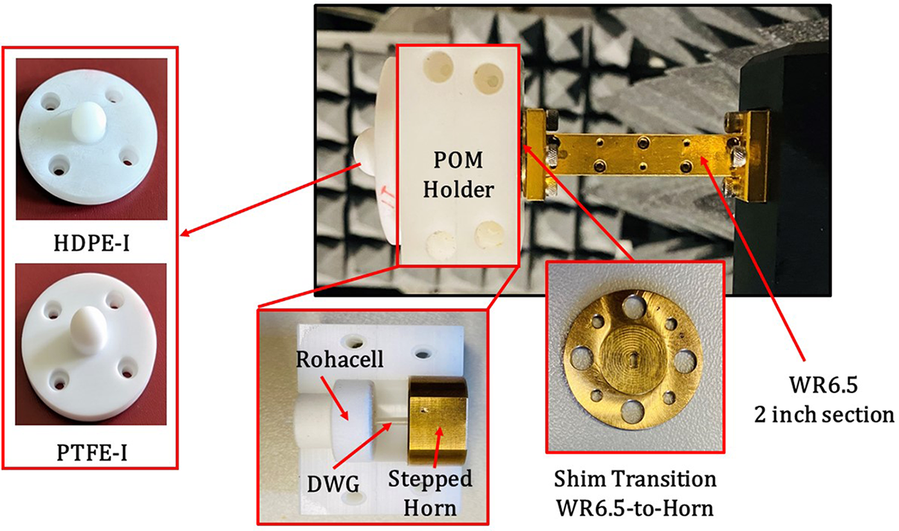
Figure 16 Long description
The image displays HDPE-I and PTFE-I prototypes, each with a distinct design. The POM holder is centrally positioned, connected to a WR6.5 two-inch section. The Rohacell material is visible alongside the DWG and stepped horn. A shim transition labeled WR6.5-to-Horn is shown, indicating the connection between components. The setup is detailed with annotations pointing to each part, highlighting the structural arrangement and material usage.
Dimensions of the fabricated lenses (all values in  $\mathrm{mm}$)

Table 1 Long description
The table presents dimensions of fabricated lenses, including contour type, diameter, depth, extension, and insertion. PTFE-II-E and PTFE-III-E lenses have elliptical contours, with PTFE-III-E showing the largest depth at 13.4 mm. Spherical arc lenses, such as HDPE-I, PTFE-I, and PTFE-II-S, have smaller depths, ranging from 4.1 mm to 4.4 mm. Diameter is consistent at 10.6 mm for PTFE-I, PTFE-II-S, and PTFE-II-E, while PTFE-III-S and PTFE-III-E have a larger diameter of 20.0 mm. Insertion is absent for HDPE-I and PTFE-I but present for PTFE-II-S, PTFE-II-E, PTFE-III-S, and PTFE-III-E, with values of 5.0 mm and 8.0 mm respectively. The data suggests that elliptical lenses tend to have larger dimensions compared to spherical arc lenses.
Manufactured lens antenna prototypes of PTFE-II-S, PTFE-II-E, PTFE-III-S and PTFE-III-E with CDWG inserted into PTFE-III-E.
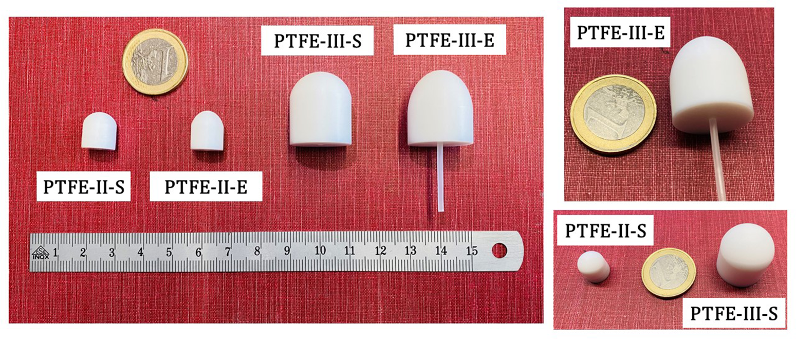
Figure 17 Long description
The image shows three PTFE lens antenna prototypes labeled PTFE-II-S, PTFE-II-E, PTFE-III-S and PTFE-III-E. The prototypes are positioned next to a ruler for scale and coins for size comparison. The PTFE-II-S and PTFE-II-E are smaller, while PTFE-III-S and PTFE-III-E are larger with a cylindrical extension. The ruler provides measurements in centimeters and the coins offer a visual reference for the dimensions of the prototypes. The setup is displayed on a textured surface.
Experimental validation
The full-wave simulations do give an idea about the performance of the lens antennas but a verification of the results and the quantification of the performances in real world through measurements is a must. For the validation of the antennas, the matching, the gain, and the radiation patterns are measured.
Return loss measurement
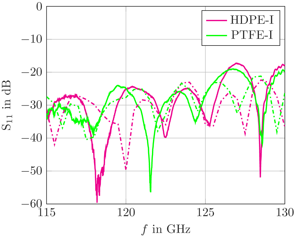
Measured ( $-$) and simulated ( $-\cdot$) $\text{S}_{11}$ in $\mathrm{dB}$ for the two different lens antennas under test HDPE-I, PTFE-I.
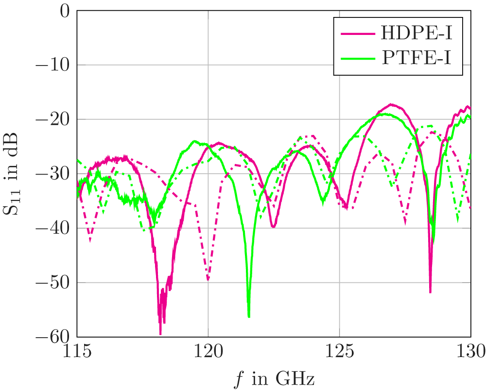
Figure 18 Long description
The graph shows reflection coefficients S subscript 11 in dB plotted against frequency f in GHz, ranging from 115 to 130 GHz. Two curves are present: one for HDPE-I and another for PTFE-I antennas. The HDPE-I curve is represented by a solid line, while the PTFE-I curve is shown with a dashed line. Both curves exhibit multiple peaks and troughs, indicating variations in reflection coefficients across the frequency range. The values on the y-axis range from 0 to negative 60 dB, with the curves generally staying below negative 20 dB, demonstrating the performance of the antennas in terms of reflection coefficients over the specified frequency range.
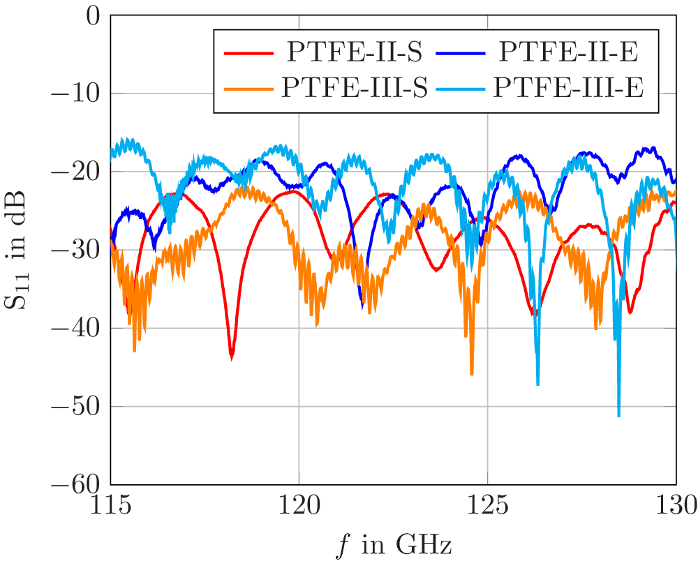
Measured  $\text{S}_{11}$ in $\mathrm{dB}$ for the different lens antennas under test PTFE-II-S, PTFE-II-E, PTFE-III-S and PTFE-III-E.
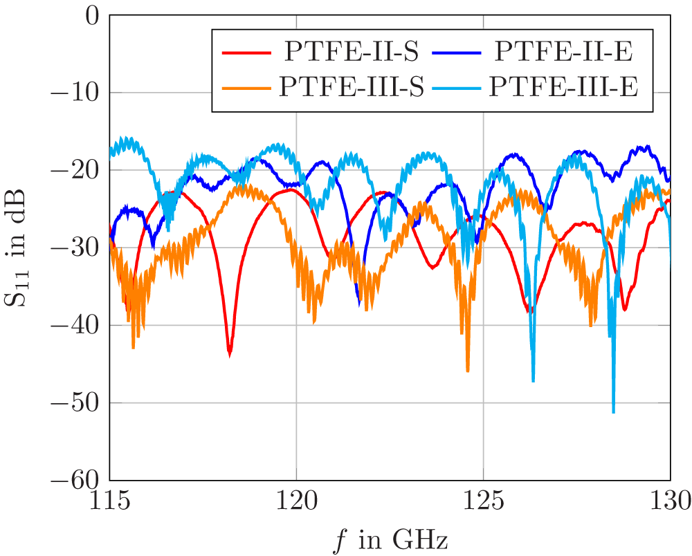
Figure 19 Long description
The graph displays the reflection coefficients S subscript 11 in decibels plotted against frequency f in gigahertz. Four curves represent different lens antennas: PTFE-II-S, PTFE-II-E, PTFE-III-S and PTFE-III-E. The x-axis is labeled as f in GHz, ranging from 115 to 130 GHz. The y-axis is labeled as S subscript 11 in dB, ranging from 0 to negative 60 dB. Each curve shows variations in reflection coefficients across the frequency range, indicating performance differences among the antennas.
B2B measurement setups with variable attenuator between the uncalibrated measuring heads in anechoic chamber (left) and the calibrated measuring heads of the VNA (right) to exactly characterize the variable attenuator.
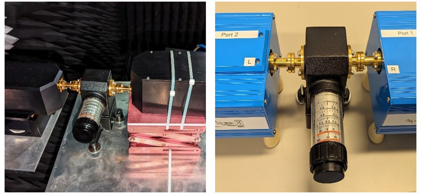
Figure 20 Long description
The image A shows a measurement setup in an anechoic chamber. It includes a variable attenuator connected between two measuring heads. The environment is designed to minimize reflections and external noise. The image B shows a similar setup with a variable attenuator between two measuring heads labeled 'Port 2' and 'Port 1'. This setup is in a different environment, possibly a laboratory setting, with clear labels on the equipment. Both setups feature similar components but are situated in distinct environments for different measurement purposes.
The matching of the antennas is measured by measuring the S-parameters with a VNA using D-band measuring heads calibrated at the WR6.5 plane. Conical absorbing walls are kept at a distance from the antenna to reduce any additional reflections. The measured reflection coefficients of the antennas HDPE-I and PTFE-I can be seen in Fig. 18. The measurements include the matching of the transition together with the CDWG and the lens antenna. Simulated reflection coefficients (with the transition, CDWG, holder, and the lens with losses) are also plotted, which suggests that the measurements tally closely with the simulations. It is observed that the reflection coefficients  $\text{S}_{11}$ for all the antennas are below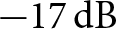 $-17\,\mathrm{dB}$ in the overall range and is actually even $ \lt -22\,\mathrm{dB}$ up to $126\,\mathrm{GHz}$. The measured reflection coefficients of the other four prototypes are shown in Fig. 19. Here also, the matching is quite good with $\text{S}_{11} \lt -20\,\mathrm{dB}$ throughout. As expected from the previously done simulative analysis (see section “Simulative analysis”), the spherical arc contour-based lenses (PTFE-II-S) outperform the elliptical contour-based lens (PTFE-II-E). This can be seen for both the smaller (PTFE-II series) and the larger (PTFE-III series) lens antennas. However, still these results are approx. $7\,\mathrm{dB}$ better than of the other elliptical lens antenna (without an extension) presented in [Reference Geiger, Hitzler, Iberle and Waldschmidt22]. Therefore, this transition and the CDWG fed lens antenna could be a promising simpler module that can easily integrated to system applications.
Gain measurement
There are different methods to measure the gain of an antenna such as gain-transfer method, the absolute gain method, and the three-antenna method. The basic idea of the three-antenna method is that three antennas are tested in pairs, and measurements of corresponding power ratios ( $\text{S}_{21}$) are taken. These measurements can then be used and upon solving a set of mathematical equations the gain of each antenna can be found out [Reference Xiao, Pan and Zhenfei40], [Reference Shakhtour, Cornelius and Heberling41]. For this work, a similar three-antenna method is used, however, the power ratios that are measured are from an un-calibrated system. This means that the power that is fed to the Tx antenna is not fixed (and unknown) and it also varies strongly over the frequency. Therefore, these power levels cannot directly be used to calculate the gain factors. To mitigate this issue, a strategical work around is proposed. At first, a back-to-back measurement is taken by connecting the Tx and Rx port. Of course in free space one would have the free space path loss, so to replicate that, a variable attenuator is added in between the Tx and Rx. This same back-to-back setup is measured with the help of a calibrated VNA to exactly characterize the variable attenuator for different attenuation settings. Both setups can be seen in left and right sides of Fig. 20, respectively. Once all the readings are taken, a correction factor for each frequency is generated. This correction factor is used in the calculations with the measured power ratios to be able to use them for the actual antenna gain calculations. By this, one can eliminate the need for a known reference antenna (standard gain horn) and a calibrated Tx port. Since three antennas are needed to measure the different antennas under test, two other commercially available pyramidal rectangular horn antennas are used that have dimensions of approx. $16\,\mathrm{mm} \times 12\,\mathrm{mm}$ and a very rough data sheet gain of $\approx 23.5\,\mathrm{dB}\text{i}$ at $140\,\mathrm{GHz}$.
Measurement setup
The lens antennas are measured in pairs in an anechoic chamber. The Rx antenna is rotated along the red line as can be seen in Fig. 21. The horizontal rotation gives the H-plane measurements. For E-plane measurements, the same setup is done but in that case, both the Tx and Rx are 90-degree rotated. The recorded power ratio levels (normalized with respect to the maxima) when plotted against this angle of rotation essentially give the radiation pattern. Also, the peak power ratio level values are then corrected with the correction factor and used to measure the gain of individual antennas using the three-antenna method explained above. The two lenses, HDPE-I and PTFE-I, are first individually measured each with the two standard pyramidal horn antennas. Then to verify the results another measurement is taken by taking the two lenses and one standard horn in the same setup. Similarly, the PTFE-II series lens antennas and the PTFE-III lens antennas are measured. Both the PTFE-II lens antennas (S and E) are smaller in size ergo lighter in weight, therefore, are just connected with a short CDWG section inserted inside. The antennas remain stable and the CDWG also stays straight throughout the measurements. This can be seen in Fig. 21 (right top). If needed, one can also add a small Rohacell disk in between to further increase the stability. However, in case of the PTFE-III series antennas (the larger ones) due to the weight, they tend to bend. To overcome this, the previously designed POM holder (with the rohacell disk inside) is taken just to hold the CDWG straight. The CDWG comes out of this POM holder, which is then just inserted into the large lens antenna. Due to a tight fit and the holder, now the entire setup remains stable throughout the measurements. This is also presented in Fig. 21. However, important to note that in this case, cutting the CDWG to an exact length is crucial to avoid any gap inside the lens.
Picture of different antennas under test in the anechoic chamber where a) shows the rectangular Horn antenna as Tx and for Rx side, b) shows the PTFE-I lens with the red arrow showing the rotational direction, c) shows the PTFE-II-S lens with the CDWG and d) shows the PTFE-III-S Lens with the POM holder.
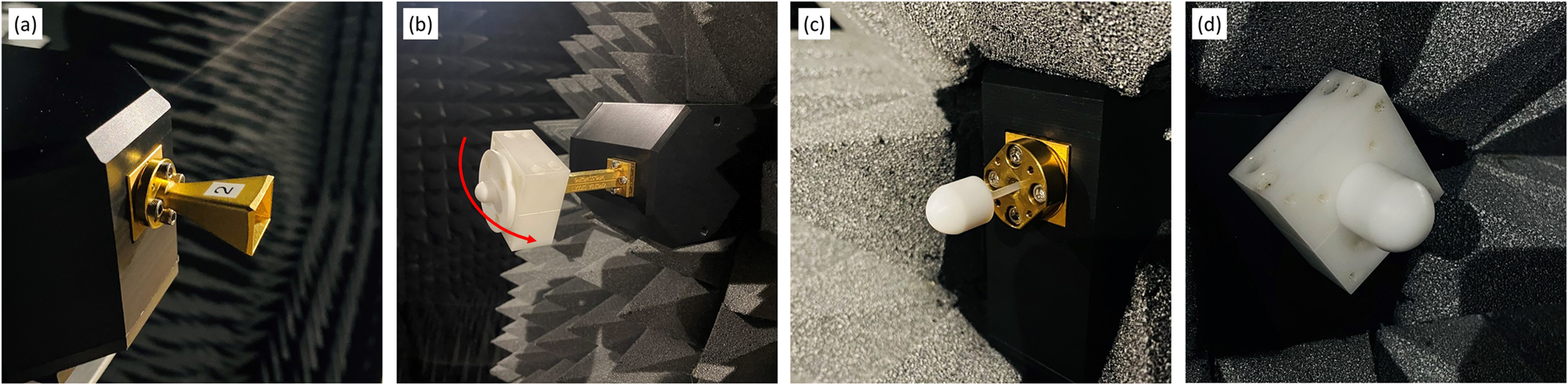
Figure 21 Long description
The first image shows the transmitter side with Horn-2, positioned in an anechoic chamber. The second image displays the PTFE-II-S lens connected with a CDWG section, also within the chamber. The third image illustrates the receiver side with a PTFE-I lens, featuring a red arrow indicating rotational direction. The fourth image presents the PTFE-III-E lens equipped with a POM holder, ensuring stability during measurements. Each setup is designed for specific pattern measurements in the chamber environment.
Measurement results
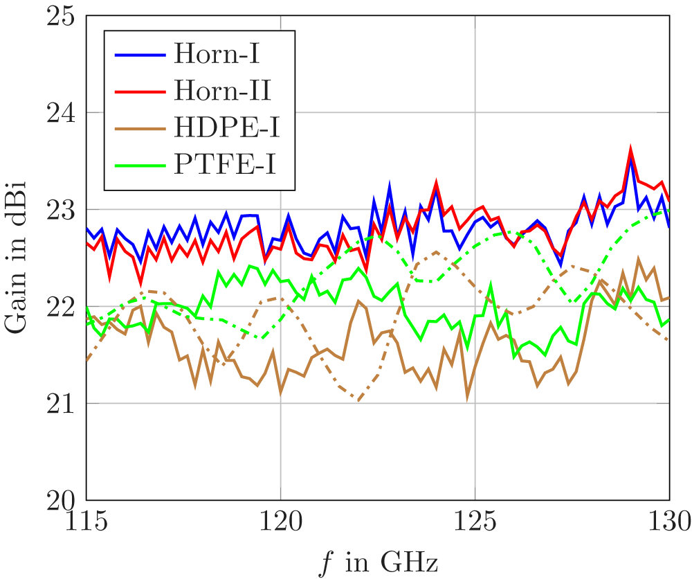
Measured ( $-$) and simulated ( $-\cdot$) gain over frequency for two horns (Horn-I, Horn-II), and the three lens antennas HDPE-I, PTFE-I, and PTFE-II.
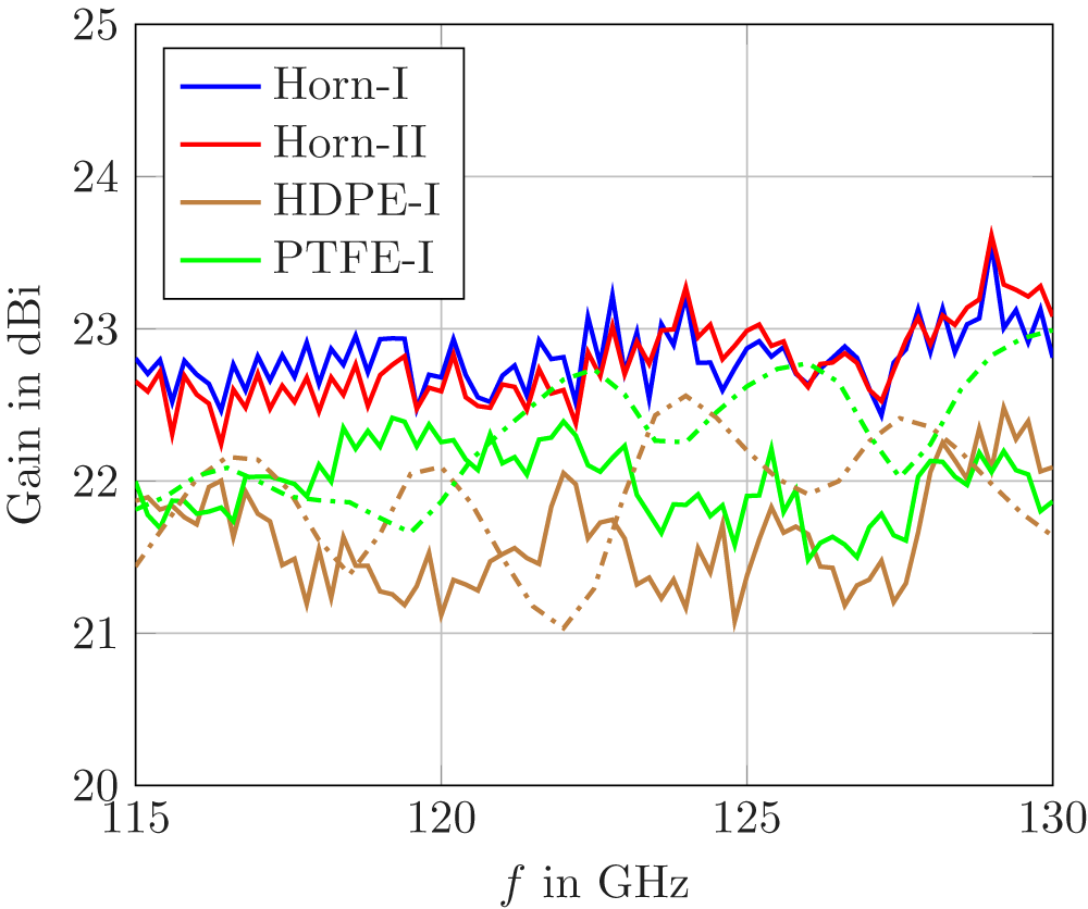
Figure 22 Long description
The graph shows gain in dBi on the y-axis and frequency in GHz on the x-axis, ranging from 115 to 130 GHz. Four curves represent different antennas: Horn-I (blue), Horn-II (red), HDPE-I (brown) and PTFE-I (green). Horn-I and Horn-II exhibit similar gain patterns, fluctuating around 23 dBi. HDPE-I shows lower gain, fluctuating around 21.5 dBi, while PTFE-I maintains a gain around 22 dBi. The graph includes dashed lines for simulated values, showing correlation with measured data.
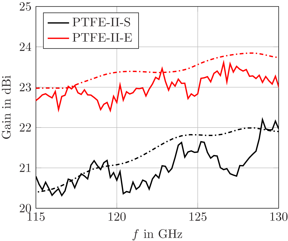
Measured ( $-$) and simulated ( $-\cdot$) gain over frequency for the lens antennas PTFE-II-E and PTFE-II-S.
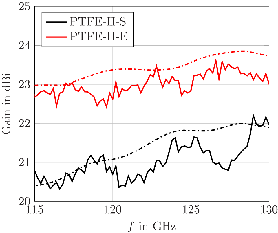
Figure 23 Long description
A line graph showing gain in dBi on the y-axis and frequency in GHz on the x-axis, ranging from 115 to 130 GHz. Two curves are plotted: PTFE-II-S represented by a solid black line and PTFE-II-E by a solid red line. The PTFE-II-S curve starts at approximately 20.5 dBi and gradually increases, peaking near 23 dBi at 130 GHz. The PTFE-II-E curve starts around 22.5 dBi and fluctuates, peaking near 24 dBi at 130 GHz. Both curves show a general upward trend with fluctuations throughout the frequency range. The graph includes dashed lines representing simulated data for both antennas, showing a similar trend to the measured data.
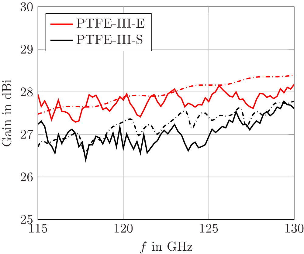
Measured ( $-$) and simulated ( $-\cdot$) gain over frequency for the lens antennas PTFE-III-E and PTFE-III-S.
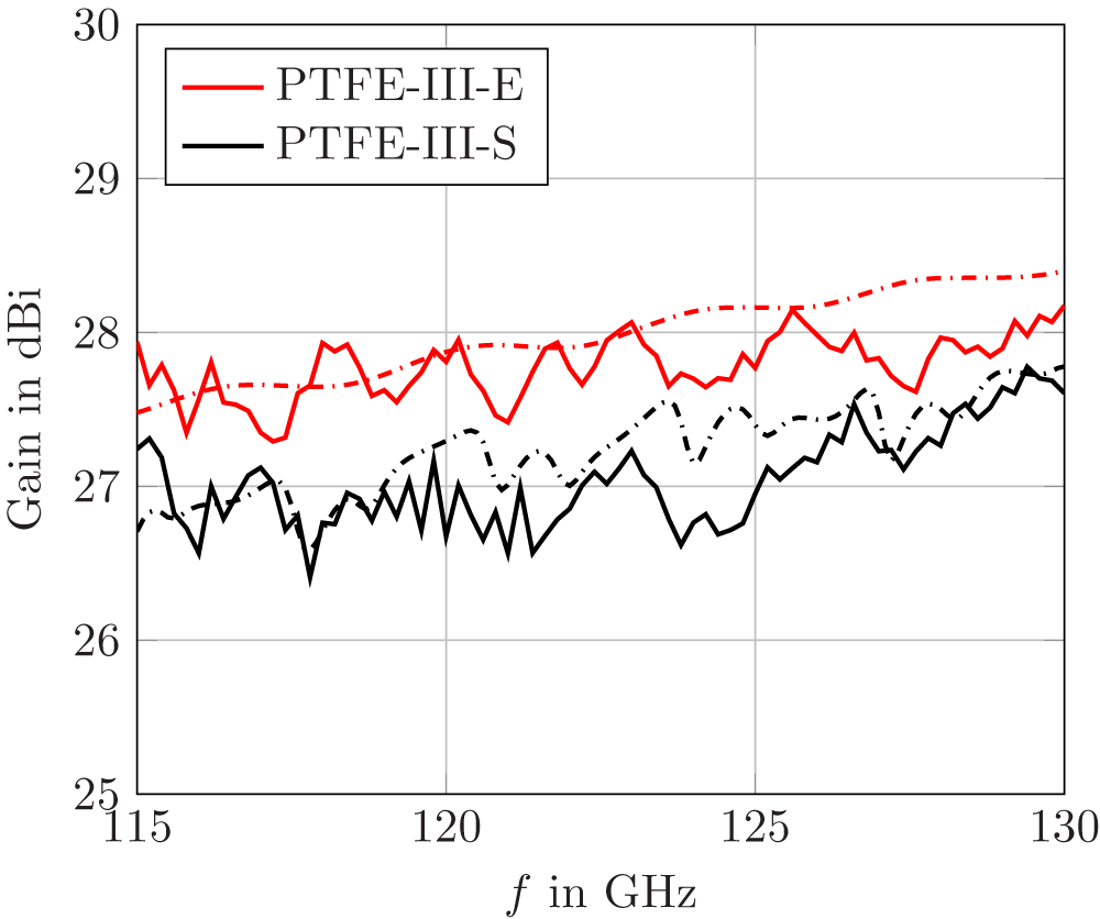
Figure 24 Long description
A line graph showing gain in dBi on the y-axis and frequency in GHz on the x-axis, ranging from 115 to 130 GHz. Two curves are plotted: PTFE-III-E and PTFE-III-S. The PTFE-III-E curve is represented with a solid line and a dot-dashed line, showing gain values fluctuating around 28 dBi. The PTFE-III-S curve is represented with a solid line and a dashed line, showing gain values fluctuating around 27 dBi. The graph includes a legend indicating the line styles for each antenna type.
The measured gain factors over frequency for the HDPE-I and PTFE-I lens antennas along with the two pyramidal horn antennas are presented in Fig. 22. Both the horn antennas show similar average gain of approx.  $22.8\,\mathrm{dB}\text{i}$. The PTFE-I shows a good performance overall with an average gain of approx. $22\,\mathrm{dB}\text{i}$ whereas the HDPE-I shows an average gain of approx. $21.5\,\mathrm{dB}\text{i}$. To compare with simulations, the simulated gain factors are also plotted (dot-dashed curves) in Fig. 22, and they show a good correlation with the measured values. In a similar fashion, the gain factors of the PTFE-II and PTFE-III lens antennas are also measured and presented in Figs. 23 and 24, respectively. Average gain of approx. $21\,\mathrm{dB}\text{i}$ and approx. $22.8\,\mathrm{dB}\text{i}$ is measured for PTFE-II-S and PTFE-II-E antennas, respectively. For the large antennas, average gains of approx. $27\,\mathrm{dB}\text{i}$ and approx.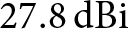 $27.8\,\mathrm{dB}\text{i}$ are measured for PTFE-III-S and PTFE-III-E antennas, respectively. All the measured gain factors do include the losses of the transition from WR6.5 to CDWG and the losses of the CDWG sections. It can be seen from both the figures that the gain of the elliptical contour-based lens antennas has a better performance with respect to the gain unlike with respect to the matching. This meets with the expectation from the simulative analysis. It is important to note that the measured gain values can deviate from the simulated ones by up to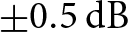 $\pm0.5\,\mathrm{dB}$. This is due to the mechanical and other physical limitations of the measurement equipment. In both the gain vs. frequency plots (Figs. 23 and 24) the deviations are within this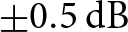 $\pm0.5\,\mathrm{dB}$ range. Additionally, the demand for the flat smooth cut of the CDWG might limit the performance of the lens antennas. It can also be seen that the gain fluctuations over frequency are less for the standard horn antennas whereas it is more for the lens antennas. A similar variation is also seen in simulations because of the presence of the flange and holder structure and multiple reflections. This reduces the case when the CDWG is just inserted instead of using a flange.
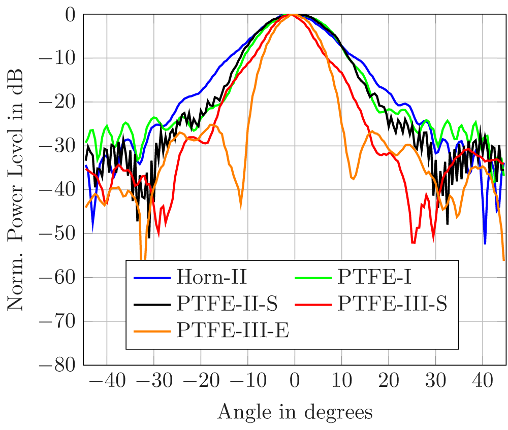
Measured normalized radiation pattern in H-plane for Horn-II, PTFE-II-S, PTFE-III-S and PTFE-III-E at  $125\,\mathrm{GHz}$ when Horn-I is kept at the transmitter.
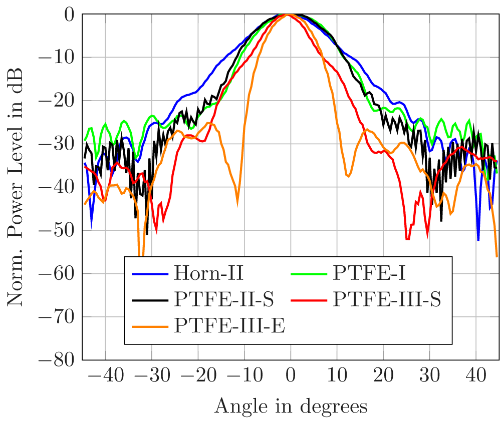
Figure 25 Long description
A line graph showing normalized power levels in decibels on the y-axis versus angle in degrees on the x-axis. The graph includes five curves representing different antennas: Horn-II, PTFE-I, PTFE-II-S, PTFE-III-S and PTFE-III-E. The Horn-II curve is plotted in blue, PTFE-I in green, PTFE-II-S in black, PTFE-III-S in red and PTFE-III-E in orange. The graph displays variations in power levels across angles ranging from negative 40 to positive 40 degrees. Each curve shows distinct patterns, with peaks and troughs indicating changes in power levels at different angles.
Radiation pattern and efficiency
The measured normalized H-plane radiation patterns at  $125\,\mathrm{GHz}$ are plotted in Fig. 25 for the different antennas when they are kept as receiver, and Horn-I is kept as transmitter. These plots are normalized to their respective maximum values since they are taken from uncalibrated measurements. The patterns for Horn-II, PTFE-I, and PTFE-II-S lens antenna are plotted to point out the difference between an antenna with flange (PTFE-I) and one with the CDWG inserted inside, also comparing to a standard horn. To differentiate between the spherical and elliptical contours and also between the large and small antennas, the radiation pattern for PTFE-III-S and PTFE-III-E is also plotted in the same Fig. 25. It can be clearly seen that for a larger lens antenna the main beam becomes narrow ergo, more gain is obtained. The difference between the radiations of different contours can also be seen in this figure; however, the difference is not very significant.
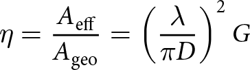
Another important metric to quantify the performance of such lens antennas is the aperture efficiency. For a particular frequency, the aperture efficiency is related to the gain and the diameter of the antenna via the following relation:
 \begin{equation}
\eta = \frac{A_\text{eff}}{A_\text{geo}} = \left({\frac{\lambda}{\pi D}}\right)^2 G
\end{equation}
\begin{equation}
\eta = \frac{A_\text{eff}}{A_\text{geo}} = \left({\frac{\lambda}{\pi D}}\right)^2 G
\end{equation}The aperture efficiency (the ratio between effective area and geometrical area) gives an idea about how homogeneously the corresponding phase delays for all rays equate to each other, ultimately giving a plane wavefront in the front of the lens antenna. This strongly determines the peak gain factors.
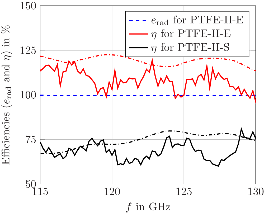
Measured ( $-$) and simulated ( $-\cdot$) aperture efficiency ( $\eta$) over frequency for the lens antennas PTFE-II-E and PTFE-II-S along with the simulated radiation efficiency ( $e_\text{rad}$) ( $--$) over frequency for PTFE-II-E lens antenna.
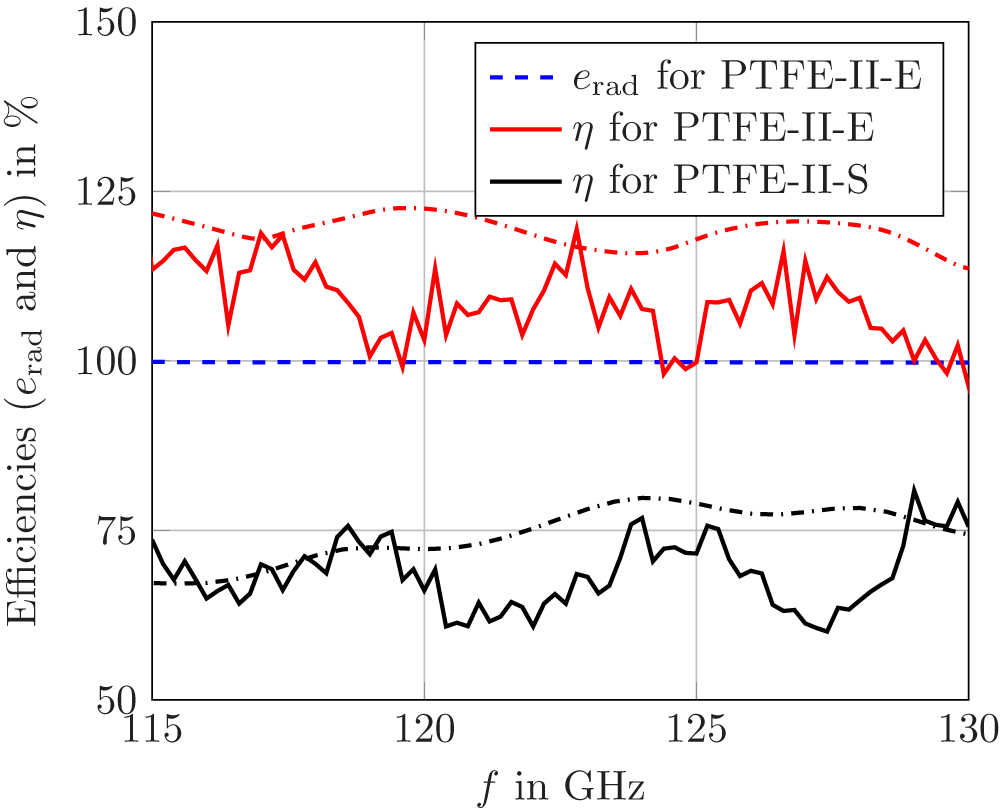
Figure 26 Long description
The graph displays efficiencies in percentage for PTFE-II-E and PTFE-II-S lens antennas over a frequency range from 115 to 130 GHz. The y-axis is labeled 'Efficiencies (e subscript rad and eta) in percent' and the x-axis is labeled 'f in GHz'. Three curves are shown: a dashed blue line representing e subscript rad for PTFE-II-E, a solid red line representing eta for PTFE-II-E and a dashed black line representing eta for PTFE-II-S. The red curve fluctuates around 100 percent, while the black curve remains below 100 percent. The blue line is constant at 100 percent. A section of the graph is obscured, affecting the visibility of some data points in the black curve.
From the measured gain factors and using eq. (9), the aperture efficiency at  $125\,\mathrm{GHz}$ is calculated to be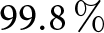 $99.8\,\%$ and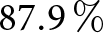 $87.9\,\%$ for the elliptical contour based lens with diameter of $10.6\,\mathrm{mm}$ and $20.0\,\mathrm{mm}$, respectively. But this is only for one frequency point (at $125\,\mathrm{GHz}$). It is important to observe the aperture efficiency over the entire frequency range. The simulated and measured gain factors over frequency are used to calculate the $\eta$ over frequency for PTFE-II-E and PTFE-II-S lens antennas. This is demonstrated in Fig. 26. From this plot it can be noticed that it is possible to have an aperture efficiency more than 100%, like in case of PTFE-II-E. The deviation of the measured values from the simulated values is within the measurement setup’s limited precision. From Fig. 26, it can be also noticed that for the spherical contour based lens, the $\eta$ is much lower than the elliptical one which is also expected from the contour derivation shown in section “Derivation of the lens contour”. This is because for the aperture efficiency calculations, the area of the circular aperture is only considered as the geometric area. However, for such lenses with its extension along the direction of propagation, the entire structure (in 3D) is responsible for radiations and not only the 2D circular face, that is how they end up delivering higher gain. Such antennas are thereby sometimes also termed as super gain antennas.
Apart from aperture efficiency, another key parameter worth exploring is the radiation efficiency ( $e_\text{rad}$). As per definition, $e_\text{rad}$ is basically the ratio between the gain and the directivity. In this case, this can be calculated from the ratio between the gain factors obtained under lossy and lossless conditions. Since the dielectric lenses used here are quite small and are made of PTFE which has a very low loss tangent, it is imperative to say that the radiation efficiency is quite high (here,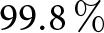 $99.8\,\%$). Moreover, under simulation environment this is constant over the desired frequency range. This can be also seen in Fig. 26 where the simulated $e_\text{rad}$ is plotted over frequency for PTFE-II-E as an example. In practical scenario, this might vary very slightly over frequency (depending on how much the loss tangent of the material vary over frequency) but still the overall value would remain quite high as the lenses are quite small and the loss tangent is very low. An overview of the key results (gain, match, and aperture efficiency) obtained for all the prototypes is shown in Table 2. It is worth to mention that the used metallic horn antennas have an aperture efficiency of only approx. $47\%$ at $125\,\mathrm{GHz}$. With this aperture efficiency and maintaining the same aspect ratio, to achieve a gain of $27.8\,\mathrm{dB}$i (as measured for the $20\,\mathrm{mm}$ PTFE-III-E lens), the metallic horn would have a size of approx.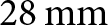 $28\,\mathrm{mm}$ x $21\,\mathrm{mm}$. This shows that the dielectric lens antennas typically have a greater efficiency than conventional metallic horn antennas.
Quantitative overview of the measured average gain (in the range of  $115-130\,\mathrm{GHz}$), gain at $125\,\mathrm{GHz}$, return loss, and the aperture efficiency (at $125\,\mathrm{GHz}$) for all the antenna prototypes

Table 2 Long description
The table compares various metrics for different antenna prototypes, including diameter, average gain, gain at 125 GHz, return loss, and aperture efficiency. PTFE-II-E has the highest aperture efficiency at 99.8%, indicating superior performance at 125 GHz. PTFE-III-E exhibits the highest average gain at 27.8 dBi, suggesting strong signal amplification. PTFE-II-S and PTFE-III-S have the same diameter of 10.6 mm, but PTFE-III-S has a significantly higher average gain of 27.0 dBi compared to PTFE-II-S's 21.1 dBi. Return loss varies across prototypes, with PTFE-I and PTFE-III-E both at 17 dB, while PTFE-II-S and PTFE-III-S are at 22 dB, indicating better impedance matching. The data suggests that larger diameter antennas tend to have higher gains and efficiencies.
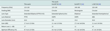
Another important characteristic worth mentioning here is polarization of the antenna. Here, the antenna is excited by the  $\text{HE}_{\text{11}}$ mode of the CDWG that is excited from the rectangular waveguide. This suggests that the antenna emits a linearly polarized wave. This is proved by the axial ratio measurement conducted in the anechoic chamber. An axial ratio of $ \gt 40\,\mathrm{dB}$ is measured throughout the frequency range depicting a linear polarized wave radiation. However, since a structural symmetry exists in the overall structure, the antenna is able to emit any polarization, if the particular polarization is properly excited into the CDWG. A comparison is also made between the achieved results and the existing state-of-the-art found from literature survey. The comparison is made on the basis of few physical factors like feeding techniques, lens types, and materials, and on the basis of performance metrics like gain, matching, and aperture efficiency. The comparison is presented in Table 3.
Comparison of the achieved results (at center frequency) with articles on D-band lens antennas with DWG feeding
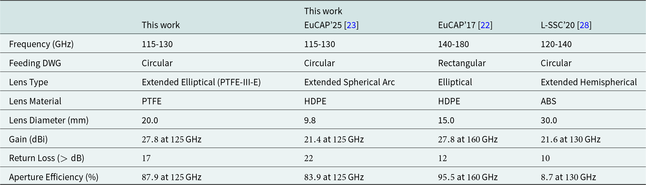
Table 3 Long description
The table compares the performance of D-band lens antennas with different feeding and lens types across various studies. It includes frequency ranges, feeding DWG types, lens types and materials, lens diameters, gain, return loss, and aperture efficiency. Notably, the PTFE-III-E lens in this work achieves a gain of 27.8 dBi at 125 GHz, while the HDPE lens in EuCAP’17 achieves a 95.5% aperture efficiency at 160 GHz. The lens diameters vary significantly, with the largest being 30.0 mm for the ABS lens in L-SSC’20. Return loss is highest at 22 dB for the HDPE lens in EuCAP’25. The table highlights the trade-offs between gain, efficiency, and material properties in lens antenna design.
Conclusion
In this study, a design strategy, various simulative analyses, and laboratory validations are detailed that guide one to design a dielectric lens antenna fed by a CDWG. The work brings in the inherent advantage of low-loss flexible dielectric waveguides in D-band frequencies and the necessity of high-gain lens antennas together into a bundle that one can tweak to ones need and integrate easily into systems. First, a simple plug-n-play transition structure is proposed that launches the guided mode into the CDWG from standard equipment connections. A measured return loss better than  $25\,\mathrm{dB}$ and low insertion loss of only $0.2..0.3\,\mathrm{dB}$ per transition is obtained in the frequency range of $115-130\,\mathrm{GHz}$. Following that, the ray optics and the geometrical structure equations are exploited to derive the lens contour. It is found that the elliptical contoured lens could be the key to the question. However, to validate it and compare it with other contour shapes, various full-wave simulations are conducted. Key design insights are provided where one can have a trade-off between the matching and gain to find a suitable design for a particular application. Based on the simulative analysis, different antenna prototypes covering different contours, different sizes ( $D=10.6\,\mathrm{mm}$ and $D=20.0\,\mathrm{mm}$) are manufactured using CNC milling on materials like HDPE and PTFE. In case of some PTFE lenses the CDWG is directly inserted into the lens removing the need for support structures. The antennas are quite small, compact, and easy to integrate, which makes it quite advantageous for many systems. However, even with the small aperture size (diameter of $10.6\,\mathrm{mm}$), the antenna is able to achieve a high gain of $22\,\mathrm{dB}\text{i}$. If one needs even higher gain factors than with a diameter of $20.0\,\mathrm{mm}$, a gain of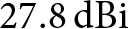 $27.8\,\mathrm{dB}\text{i}$ is obtained. These could really boost up the power level and meet the requirements of the link budget, especially in advanced radar systems where the antenna could be relocated flexibly to a different position, and the loss along the path could be compensated by the high gain of the antennas.
Acknowledgements
We sincerely acknowledge the support and funding from the DistriMuSe project under the HORIZON-KDT-JU-2023-2-RIA call. It is co-funded by the EU under grant agreement 101139769 and German national funding agency BMBF under grant agreement 16MEE0429.
Competing interests
The author(s) declare none.

Abhijit Pal received his B.Tech degree in Electronics and Communications Engineering from Heritage Institute of Technology, Kolkata, India, in 2017, and his M.Sc. degree in Communication and Information Technology from the University of Bremen, Germany, in 2021. Since then, he has been working as a Research Engineer at the RF & Microwave Engineering Laboratory of the University of Bremen, Germany. He is currently pursuing his Ph.D. degree there, focusing on research in the field of communication and radar sensing systems with dielectric waveguides.

Debrina Dutta received her B.Tech degree in Electronics and Communications Engineering from Future Institute of Engineering and Management, Kolkata, India, in 2019, and her M.Sc. degree in Communication and Information Technology from the University of Bremen, Germany. In December 2025, she started to pursue a Ph.D. degree at the RF & Microwave Engineering Laboratory, University of Bremen.

Martin Schneider received his Diploma and Doctorate degrees in Electrical Engineering from the University of Hanover, Germany, in 1992 and 1997, respectively. From 1997 to 1999, he was with Bosch Telecom GmbH, where he developed microwave components for point-to-point and point-to-multipoint radio link systems. In November 1999, he joined the Corporate Research division of Robert Bosch GmbH. As a project and section manager of the “Wireless Systems” group, he focused on research and development of smart antenna concepts for automotive radar sensors at 24 and 77 GHz. From 2005 to 2006, he was with the business unit “Automotive Electronics” of Robert Bosch GmbH, where he was responsible for the “RF electronics” of automotive radar sensors. Since March 2006, he has been a Full Professor and Head of the RF & Microwave Engineering Laboratory at the University of Bremen (Germany).






































 Open access

