


1. Introduction
Current glacier retreat is unprecedented considering the last 2000 years (IPCC, 2023). Global glacier mass loss is projected to continue into the 21st century in response to climate change and is linearly related to temperature change (Edwards and others, Reference Edwards2021; Rounce and others, Reference Rounce2023). Glaciers have been and will continue to be a major source of sea level rise in the 21st century (e.g. Frederikse and others, Reference Frederikse2020; Edwards and others, Reference Edwards2021; IPCC, 2023). Glaciers are also important regulators of water availability in many regions of the world (Kaser and others, Reference Kaser, Grosshauser and Marzeion2010; Huss and Hock, Reference Huss and Hock2018) and glacial runoff can potentially buffer droughts (Pritchard, Reference Pritchard2019) even in regions where runoff declines over the 21st century (Ultee and others, Reference Ultee, Coats and Mackay2022). Improving glacier evolution models is thus critical to better understand how glaciers will respond to climate change and enhance the accuracy of predictions regarding associated impacts.
The Glacier Model Intercomparison Project Phase 2 (GlacierMIP2, Marzeion and others, Reference Marzeion2020) partitioned various sources of uncertainty and found that the primary source of uncertainties of our projections in the first half of the century comes from differences in the glacier models. However, the study could not disentangle the choices in model design nor the specific processes responsible for these discrepancies. Our study focuses on a central component of glacier evolution models (Zekollari and others, Reference Zekollari, Huss, Farinotti and Lhermitte2022): the mass-balance (MB) model and its calibration.
Most large-scale glacier models (9 out of 11 models in GlacierMIP2) require only temperature and precipitation climate data. Accumulation is estimated by snowfall (i.e. precipitation below a certain temperature threshold) and ablation by temperature-index models (e.g. Hock, Reference Hock2003), where melt is computed by multiplying a calibrated degree-day factor by the sum of temperatures above a chosen threshold. This simple but reliable approach is still prevalent due to significant uncertainties in the local climate forcings and a lack of temporally and spatially-resolved MB observations that would be necessary to calibrate the free parameters in more complex MB models.
The temperature-index models (in the following referring to the ablation and accumulation part of the MB model) used in the literature vary based on their temporal resolution, climate downscaling approaches, representation of surface conditions and the processes that are explicitly modelled. While some temperature-index models of large-scale studies use monthly climate data (Marzeion and Hofer, Reference Marzeion, Jarosch and Hofer2012; Maussion and others, Reference Maussion2019; Rounce and others, Reference Rounce2020b), others also include the daily temperature standard deviation (Anderson and Mackintosh, Reference Anderson and Mackintosh2012; Huss and Hock, Reference Huss and Hock2015; Zekollari and others, Reference Zekollari, Huss and Farinotti2019). Recent General Circulation Models (GCMs) (e.g. ISIMIP3b, Lange, Reference Lange2019) provide daily data, opening opportunities to evaluate the impact of temporal resolution of forcing data on glacier projections. Some models use different degree-day factors for different surface types (e.g. snow, firn, ice and debris cover; Radić and others, Reference Radić2014; Huss and Hock, Reference Huss and Hock2015; Zekollari and others, Reference Zekollari, Huss and Farinotti2019; Rounce and others, Reference Rounce, Hock and Shean2020a, Reference Rounce2020b; Compagno and others, Reference Compagno2022), while others do not (Marzeion and Hofer, Reference Marzeion, Jarosch and Hofer2012; Maussion and others, Reference Maussion2019). Distinguishing surface types is more realistic, as the degree-day factor of snow is generally smaller than that of ice to account for the difference in albedo (e.g. Braithwaite, Reference Braithwaite2008); however, this distinction introduces more unknown parameters. Additionally, using two or three surface types may not realistically represent the continuous evolution of albedo during summer melt (Marshall and Miller, Reference Marshall and Miller2020). To our knowledge, no systematic comparison of these temperature-index model variants has been performed for data-scarce situations typical of large-scale studies where hundreds or thousands of glaciers are considered at once.
In previous model intercomparisons, the calibration data also varied considerably by model, ranging from using in-situ direct glaciological observations from the WGMS (2020) for about 300 glaciers (e.g. Marzeion and Hofer, Reference Marzeion, Jarosch and Hofer2012; Maussion and others, Reference Maussion2019; Shannon and Others, Reference Shannon2019) to regional mean satellite geodetic MB estimates (e.g. Anderson and Mackintosh, Reference Anderson and Mackintosh2012; Huss and Hock, Reference Huss and Hock2015; Sakai and Fujita, Reference Sakai and Fujita2017). The different methods used to extrapolate the calibrated parameters between glaciers result in large uncertainties (e.g. Maussion and others, Reference Maussion2019). Using glacier-specific, instead of regional, mean geodetic MB estimates can capture sub-regional spatial variability and offers unprecedented opportunities for model calibration (Zekollari and others, Reference Zekollari, Huss and Farinotti2019; Rounce and others, Reference Rounce2020b; Compagno and others, Reference Compagno, Zekollari, Huss and Farinotti2021; Rounce and others, Reference Rounce2023). The global geodetic glacier dataset of Hugonnet and others (Reference Hugonnet2021) provides a mean specific glacier MB estimate between 2000 and 2019 for almost every glacier on Earth (>200 000 glaciers). Although Hugonnet and others (Reference Hugonnet2021) also provide annual estimates, the uncertainties are too large to be used. By changing only one model option (i.e. a temperature-index model choice or calibration strategy) at a time within the Open Global Glacier Model (OGGM) framework, we provide insight into glacier model behaviour differences that cannot be captured in large-scale glacier model intercomparisons.
Since glacier evolution models have multiple MB model parameters, the use of a single observation per glacier for calibration causes the model to be overparameterised (Rounce and others, Reference Rounce2020b) and results in multiple combinations of MB model parameters providing similar agreement between the model and observations (equifinality). This problem is usually ignored by either fixing global parameters (Marzeion and Hofer, Reference Marzeion, Jarosch and Hofer2012; Maussion and others, Reference Maussion2019) or by selecting parameter values sequentially in order of their expected uncertainty (Huss and Hock, Reference Huss and Hock2015; Zekollari and others, Reference Zekollari, Huss and Farinotti2019; Compagno and others, Reference Compagno, Zekollari, Huss and Farinotti2021). A first attempt to estimate the uncertainty arising from equifinality was implemented in Rounce and others (Reference Rounce, Hock and Shean2020a, Reference Rounce2020b) using an empirical Bayesian inverse model, which has the advantage of taking both the equifinality and observational uncertainties into account.
We aim to systematically assess the impact of specific model design choices on both the calibration procedure and glacier change projections. Specifically, we seek to determine the potential added value of more complex temperature-index model variants over simpler and less parameterised approaches. Our model options include the temperature-index model choices of the temporal resolution of climate data (monthly or daily), near-surface temperature lapse rates and surface-type dependent degree-day factors, as well as the calibration strategies of up to three free temperature-index model parameters. We focus on 88 glaciers with long-term observations of annual, seasonal and, in some instances, elevation-dependent climatic mass balance from the WGMS (2020). Our study concludes with insights into the future potential of model calibration based on soon-to-be available data sources (e.g. Miles and others, Reference Miles2021; Jakob and Gourmelen, Reference Jakob and Gourmelen2023).
2. Input Data and Methods
2.1. Model setup and input data
2.1.1. OGGM setup
We use the open-source numerical modelling framework OGGM (Maussion and others, Reference Maussion2019), which has been applied in several global and regional studies (e.g. Furian and others, Reference Furian, Maussion and Schneider2022; Gangadharan and others, Reference Gangadharan2022; Li and others, Reference Li2022; Yang and others, Reference Yang, Li, Liu and Chu2022; Malles and others, Reference Malles2023, for most recent examples) and is well suited for our model intercomparison thanks to its modular structure. Here, we focus on the changes made to OGGM's default configuration as of version 1.5.3. For this study, OGGM uses glacier outlines from the Randolph Glacier Inventory (RGIv6.0, Pfeffer and others, Reference Pfeffer2014) and a digital elevation model to derive elevation-band flowlines (as in Huss and Farinotti, Reference Huss and Farinotti2012; Zekollari and others, Reference Zekollari, Huss and Farinotti2019; Werder and others, Reference Werder, Huss, Paul, Dehecq and Farinotti2020). We favour elevation-band flowlines (e.g. as in Malles and others, Reference Malles2023) over multiple geometrical centerlines (also available in OGGM, Maussion and others, Reference Maussion2019) as they are computationally cheaper and simplify the calibration. Glacier dynamics are represented by a 1D shallow-ice flowline model in OGGM assuming a trapezoid bed shape. Ice thickness is estimated by applying a mass-conservation approach (Farinotti and others, Reference Farinotti, Huss, Bauder, Funk and Truffer2009, Reference Farinotti2019; Maussion and others, Reference Maussion2019) and assuming the glacier outline and digital elevation model have the same date. For this study, we calibrate the creep parameter A individually for each glacier and for each temperature-index model and calibration option (see Fig. S1) to match the ice volume estimates of Farinotti and others (Reference Farinotti2019) for every glacier at the RGI year (for many glaciers, close to 2000). More details about the OGGM are available on the model documentation website (http://docs.oggm.org) and in Maussion and others (Reference Maussion2019).
2.1.2. General temperature-index model and parameter setup
All temperature-index model choices in this study are based on the original temperature-index model of OGGM presented in Maussion and others (Reference Maussion2019), which itself builds upon Marzeion and Hofer (Reference Marzeion, Jarosch and Hofer2012). Its formulation is similar to the majority of other large-scale models (references therein): The (monthly or daily) mass balance B i for an elevation z is estimated as

$P_i^{solid}( z)$ is the solid precipitation (kg m−2 month−1 or kg m−2 day−1), T i the air temperature ($^\circ$
 C) and t melt the temperature threshold above which melt is assumed to occur. We use t melt = 0 $^\circ$
 C for all model choices in our study instead of the OGGM default of −1 $^\circ$
 C, which was only tuned for the reference monthly model. d f is the degree-day factor of a specific surface type (kg m−2 K−1 month−1 or kg m−2 K−1 day−1). The fraction of solid precipitation is estimated from the monthly or daily mean temperature. Precipitation is assumed to be entirely solid below 0 $^\circ$
 C and all liquid above 2 $^\circ$
 C. In between, the solid precipitation proportion changes linearly.
Three free parameters characterise our temperature-index model variants. In addition to the degree-day factor, d f, which can vary for different snow ages and ice, two parameters are commonly considered as part of the temperature-index model but actually serve as local climate downscaling or bias correction tools. Precipitation is adjusted using a fixed multiplicative scaling precipitation factor (p f), and temperature is corrected by a temperature bias (t b), both assumed to be constant in time. These parameters are essential because the model would often fail to reproduce the observed glacier MB without them. Note that these model parameters serve not only as downscaling parameters but also account for local climate biases, incorporate missing MB processes (such as debris cover and avalanches), and address inaccuracies in MB observations (see Rounce and others, Reference Rounce2020b). To downscale the temperature and precipitation data for each elevation band in our temperature-index model, we utilise a temperature lapse rate and downscale the data from the nearest gridpoint (further details in Section 2.2). Unlike other models (Huss and Hock, Reference Huss and Hock2015; Rounce and others, Reference Rounce, Hock and Shean2020a), we do not apply any precipitation gradient due to the lack of observation data necessary to calibrate and justify such an approach.
2.1.3. Climate data
The W5E5v2.0 climate dataset (Lange and others, Reference Lange2021) is used for the historical period of 1979–2019, while the five primary GCMs from phase 3b of the Inter-Sectoral Impact Model Intercomparison Project (ISIMIP3b, Lange, Reference Lange2019, Reference Lange2022) are used for the future period of 2020–2100. The chosen GCMs (GFDL-ESM4, UKESM1-0-LL, MPI-ESM1-2-HR, MRI-ESM2-0, IPSL-CM6A-LR) are based on phase 6 of the Coupled Model Intercomparison Project (CMIP6, Eyring and others, Reference Eyring2016). Both W5E5 and ISIMIP3b GCMs are available at a daily resolution and have a spatial resolution of 0.5$^\circ$ over the entire globe. Generally, GCMs have to be bias-corrected to approximately coincide with the climate dataset used for model calibration. In this study, we did not apply an additional bias correction as the statistically downscaled GCMs from ISIMIP3b are already internally bias-adjusted to W5E5 over the period 1979–2014 (Lange, Reference Lange2019). Additionally, the bias adjustment from ISIMIP3b is more robust for extreme values than the “delta”-method that is commonly used in OGGM and other models (e.g. Zekollari and others, Reference Zekollari, Huss and Farinotti2019). For projections, we run the five GCMs from ISIMIP3b but only show the median output of the five glacier change simulations for the various model options, as multi-GCM uncertainty is not a focus of this study. We run the simulations for two Shared Socioeconomic Pathways (SSPs): the low-emission scenario SSP1-2.6 and the very high-emission scenario SSP5-8.5, which correspond to a global temperature increase by 2100 compared to preindustrial times of 1.7$^\circ$
 C and 4.6$^\circ$
 C and a global glacier area-weighted temperature increase of 3.1$^\circ$
 C and 8.0$^\circ$
 C, respectively.
2.1.4. Geodetic and in-situ mass balance observations
The main MB observations used for calibration are the globally available geodetic estimates from Hugonnet and others (Reference Hugonnet2021), which serve as the primary reference for global studies (Rounce and others, Reference Rounce2023). However, higher spatially and temporally resolved in-situ direct glaciological observations exist from the WGMS (2020) for around 300 glaciers. In the period of the applied climatic dataset (1979–2019), estimates of interannual MB variability of at least 10 years exist for 180 glaciers, and winter MB observations of at least five years exist for 118 glaciers. There are 95 glaciers with both sufficient winter MB and interannual MB variability data. MB profile data (with at least five years and five elevation bands) exist for 93 glaciers. These additional observations will be used to calibrate a glacier-specific precipitation factor and/or temperature bias alongside the degree-day factor.
2.2. Temperature-index model choices
In total, we explore 18 combinations of temperature-index model choices (Table 1) that we implemented into the OGGM framework and are all available to OGGM users (see Code & Data availability section).
Temperature-index model choices used in this study, summing to 18 combinations

The simplest combination denoted by italics (constant temperature lapse rate, monthly climate data and no surface-type distinction) is used as reference.
2.2.1. Temperature lapse rate choice
The temperature is adjusted to the flowline gridpoint altitude by a lapse rate. We set the temperature lapse rate either to (i) a constant value (−6.5 K km −1, reference model in OGGM) or (ii) extract it from pressure levels in ERA5 so that it is variable spatially and seasonally (i.e. we apply twelve constant monthly temperature lapse rates as in Marzeion and Hofer, Reference Marzeion, Jarosch and Hofer2012; Huss and Hock, Reference Huss and Hock2015; Rounce and others, Reference Rounce, Hock and Shean2020a).
2.2.2. Temporal climate resolution choice
Air temperature and precipitation data are used to force the model. We have three choices for the climate data based on the temporal resolution and variability (Table 1): (i) monthly data, (ii) pseudo-daily data, (iii) daily data. The monthly choice is the simplest, while the advantage of the pseudo-daily and daily choices is that melt can occur even if the monthly mean temperature is below 0$^\circ$ C.
C.
Variants of the pseudo-daily choice are currently used in large-scale temperature index models (Huss and Hock, Reference Huss and Hock2015; Zekollari and others, Reference Zekollari, Huss and Farinotti2019), while the daily choice is less used (Anderson and Mackintosh, Reference Anderson and Mackintosh2012) due to data availability. The pseudo-daily choice assumes daily temperatures are normally distributed over one month. We employ a quantile method to sample the normal distribution consistently and estimate monthly melt. To ensure comparability, we use the same method as in previous studies (e.g. in Huss and Hock, Reference Huss and Hock2015) by applying the same daily temperature standard deviation computed from the past climate (here: 2000–2019) to future climate (i.e. we apply twelve constant daily standard deviations over the entire period). Note that in a warming world, the pseudo-daily choice may overestimate daily temperature standard deviations as temperature variances are expected to decrease (specifically in the Northern Hemisphere winter, Screen, Reference Screen2014; Tamarin-Brodsky and others, Reference Tamarin-Brodsky, Hodges, Hoskins and Shepherd2020).
The daily choice estimates solid precipitation from the daily temperature, while the monthly and pseudo-daily choices derive solid precipitation from the monthly mean temperature. Hence, the monthly and pseudo-daily choices yield the same solid precipitation amount but differ in melt quantities, while the daily choice results in varying melt and solid precipitation amounts compared to the monthly choice.
2.2.3. Surface-type distinction choice
Over snow and firn surfaces, less melt occurs for the same temperature compared to bare ice surfaces due to differences in albedo (e.g. Braithwaite, Reference Braithwaite2008). We track snow age with a new snow ageing bucket system (see Appendix A.1 for more detail) to distinguish between snow, firn and ice at each elevation band, thereby enabling the use of different degree-day factors for these surface types. We assume a degree-day factor ratio of 0.5 between new snow and ice (as in Huss and Hock, Reference Huss and Hock2015; Zekollari and others, Reference Zekollari, Huss and Farinotti2019) but acknowledge that this is arbitrary (Rounce and others, Reference Rounce, Hock and Shean2020a). As the snow ages, we assume the ratio of the older snow to the ice degree-day factor increases every month, i.e., the assumed ratio of 0.5 is only applied for new snow and transitions to 1 over six years (i.e. the snow becomes ice).
The speed of how the degree-day factor transitions from snow to ice surfaces is not well known. We therefore compare three choices to determine the impact on model performance and glacier projections: (i) no degree-day factor change, (ii) a negative exponential increasing degree-day factor with snow age where 63% of the changes occur in the first year or (iii) a linearly increasing degree-day factor with snow age (Appendix, Fig. 8d). An argument for using an exponential degree-day factor transition with time is that Marshall and Miller (Reference Marshall and Miller2020) found a linear relationship between degree-day factor and albedo, and albedo can be parameterised to decay exponentially with time.
2.3. Temperature-index model calibration strategies
We developed five calibration strategies for glaciers with additional in-situ data to calibrate the three free parameters (Table 2). We set the allowed ranges of the degree-day factor to 0.33–33 kg m−2 K−1 day−1, precipitation factor to 0.1–10, and temperature bias to −8–8 K. All five strategies calibrate the temperature-index model to match the 20-year average glacier-specific geodetic observation (2000–2019) from Hugonnet and others (Reference Hugonnet2021). Two strategies also use the mean winter MB (C 1, C 2), and two use the interannual variability (standard deviation) of annual MB (C 1, C 3). The precipitation factor varies on a glacier-per-glacier level for all strategies except for C 4, and the temperature bias is non-zero only for C 1. For C 4, we use a different precipitation factor for every temperature-index model choice, which is set to be constant for all glaciers (median precipitation factor from C 3). For C 5, the precipitation factor depends on the glacier's winter precipitation based on a logarithmic relation found from C 2 between winter precipitation and glacier-specific precipitation factor (Fig. S2a). This correction is arguably more reasonable than a constant precipitation factor because locations with a high baseline precipitation value are not corrected towards unrealistic amounts (Fig. S2b). The precipitation factor in C 5 can be different for every glacier but is the same for every temperature-index model choice (Fig. S3).
Calibration strategies for glaciers with additional in-situ direct glaciological measurements from the WGMS (2020)
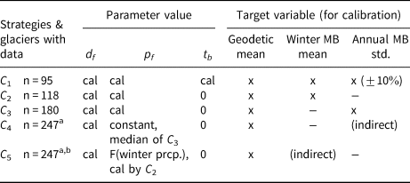
a could be applied on worldwide glaciers as it only uses the glacier-specific geodetic estimate
b Section 3.1 only uses C 5
“Cal” means this parameter is calibrated glacier-specifically, and “x” means this observational target variable is used and matched. d f stands for degree-day factor, p f for precipitation factor, t b for temperature bias, prcp. for precipitation and std. for standard deviation. For C 4 and C 5, some in-situ observational data are used for pre-calibration; they are therefore marked as “indirect”. When comparing the options, we use only the 88 glaciers that can be calibrated for all strategies and temperature-index model choices given the assumed parameter ranges.
Lower calibration strategy numbers use more observational data, thus reducing the number of glaciers that can be investigated due to calibration data availability. In Section 3.2.1, we will show that the precipitation factor influences interannual MB variability and winter MB more than the temperature bias. Therefore, we decided that C 2 and C 3 have a variable precipitation factor but do not apply any temperature bias. C 4 is similar to how the precipitation factor was calibrated in OGGM, and a variant of C 5 is the new way of calibrating the precipitation factor (OGGM v1.6).
Since we want to model the total MB to assess the impacts of glacier change (e.g. seasonal runoff and sea level rise), all calibration and temperature-index model options are tuned to match the total MB (i.e. average geodetic MB) and not the in-situ average climatic MB (the two are sometimes inconsistent for numerous reasons, e.g. Klug and others, Reference Klug2018). The in-situ data is primarily used for estimates of the interannual variability, altitude-dependent MB profile and winter MB.
In total, 88 of 95 potential glaciers with available data could be calibrated for all five calibration strategies and all temperature-index model choices when using the applied parameter ranges. All glaciers worldwide could be calibrated using C 4 and C 5. Some of the failing glaciers can be recalibrated by varying the temperature bias (not done in this study in order to enable a better comparison). We will compare the different options on the 88 common-running glaciers, of which 84 come from the Northern Hemisphere (28 from Central Europe and 19 from Scandinavia, see Fig. S4). The MB profile data is only available for 53 out of the 88 glaciers and has large uncertainties, so we only use it as an independent validation measure.
3. Model performance and climate sensitivities
Here, we explore the influence of various model options, including temperature-index model choices (Section 3.1, only using C 5) and calibration strategies (Section 3.2), on the temperature-index model output. The glacier area is assumed constant at the RGI date such that changes in glacier geometry and potential elevation change feedbacks are not considered to better isolate the differences between options.
3.1. Temperature-index model choice differences
3.1.1. Temperature-index model choice influence on calibrated parameter combinations
The calibrated parameter combinations exhibit considerable variations between the temperature-index model and calibration options. To better understand these intricate interactions, we present the disparities in model parameters for the 88 glaciers where all options could be calibrated (Fig. 1). Our emphasis lies on the calibration strategy C 5, with information for C 1−4 provided in the supplementary material (Section S1.1).
Calibrated degree-day factor (d f) for different temperature-index model choices (Table 1) using C 5 for 88 glaciers with median and interquartile range (25$\%_{\text {ile}}$ –75$\%_{\text {ile}}$
 ). Model choices have the same precipitation factor of 2.8 (median). The temperature bias is zero. Fig. S3 shows the same for all model parameters and calibration strategies.

The calibrated degree-day factor is smaller for the variable lapse rate choice than the constant choice (valid for all calibration and other temperature-index model change options, Fig. 1, Fig. S3). The variable lapse rate is, in our case, for most glaciers and months, less negative than the constant choice (median of −5.6 K km−1 versus −6.5 K km−1). Therefore, the glacier is forced with higher temperatures using the variable lapse rate choice as the lapse rate is less negative, and the glaciers are usually higher than the climate gridpoint altitudes, which explains the smaller degree-day factors.
For the three temporal climate data resolution choices, the degree-day factor is lowest for the pseudo-daily and daily data and highest for monthly data (Fig. 1). We expect a smaller degree-day factor for the pseudo-daily and daily data as melt can occur for these choices even if monthly mean temperatures are slightly below the melt temperature threshold.
For the choice without surface-type distinction, we find that the “mixed” degree-day factor (i.e. for both snow and ice) is lower than the one used for ice in models with surface-type distinction (Fig. 1). This is expected since the higher (ice) degree-day factor is only applied for ice surfaces, and a lower degree-day factor (up to a factor of 0.5) is applied for snow or firn surfaces that have a higher albedo (Section 2.2). Using a snow degree-day factor that increases faster in the first year (via a neg. exp. increase), results in a smaller ice degree-day factor than assuming a linear increase (Appendix, Fig. 8).
3.1.2. Climate sensitivities of temperature-index model choices
Despite calibrating the temperature-index model choices to the same observations, the temperature-index model choices display variable sensitivities to climate anomalies. To isolate these differences, we analyse the direct drivers of temperature-index models similar to Bolibar and others (Reference Bolibar, Rabatel, Gouttevin, Zekollari and Galiez2022); Vincent and Thibert (Reference Vincent and Thibert2023), i.e., cumulative positive degree-days (CPDD) and solid precipitation. We consider all 217 glaciers that can be calibrated under C 5 for all temperature-index model choices, assuming a fixed area over 20 years. We differentiate between temperature-induced and annual precipitation-induced MB anomalies (Figs. 2a,e). We represent their dependence on CPDD, solid winter and summer precipitation anomalies that are induced by these temperature changes (Figs. 2b–d) or annual precipitation changes (Figs. 2f–h).
MB sensitivity of (a–d) temperature and (e–h) precipitation anomalies averaged over 2000–2019 on 217 glaciers. (a) Average specific annual MB anomaly dependent on temperature bias (t b) for the ablation (melt), accumulation (solid precipitation) and their sum. (b) Translation of t b into a cumulative positive degree-day (CPDD) anomaly. (c, d) Relations of resulting solid winter and summer precipitation anomalies. (e, f, g, h) Equivalent plots for an annual precipitation anomaly solely based on changing precipitation factor (p f). This figure is inspired by Bolibar and others (Reference Bolibar, Rabatel, Gouttevin, Zekollari and Galiez2022, their Fig. 3). We use C 5 where p f of one glacier is the same for all temperature-index models and apply constant temperature lapse rates. d f stands for degree-day factor.
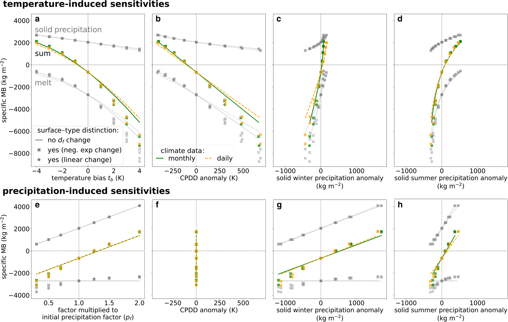
When surface-type distinction is not considered, melt increases linearly with CPDD, resulting in a nearly linear specific MB decrease (Fig. 2b). However, when applying surface-type distinction, the MB sensitivity becomes nonlinear with increased melt for larger CPDD anomalies because of increasing ice surface area. With increasing temperatures (and CPDD), the solid precipitation decreases (Figs. 2a,b). Consequently, the specific MB also strongly decreases, which is further enhanced with surface-type distinction (Figs. 2c,d). Temperature-induced negative solid winter or summer precipitation anomalies correlate in our experiment with decreasing total solid precipitation and, thus, with increasing melt. A negative temperature anomaly leads to a slight increase in solid winter precipitation (Fig. 2c), since winter precipitation is primarily solid already. The specific MB increase of temperature-induced solid winter precipitation is mainly attributed to reduced melt and increased solid summer precipitation. Conversely, the relationship between specific MB change and temperature-induced positive solid summer precipitation anomalies behaves differently with a reversed curve shape (Fig. 2d). In this case, MB sensitivities decrease as temperature-induced solid summer precipitation increases. The reason is likely that the solid summer precipitation contribution to MB increases faster than other dominant factors, such as reduced melt and increased solid winter precipitation.
Annual precipitation anomalies without temperature change affect solid precipitation, and if the degree-day factor is surface-type dependent, it also impacts melt but not CPDD (Figs. 2e,f). Surface-type distinction creates a nonlinear relationship between specific MB and precipitation-induced solid precipitation (Figs. 2g,h). With decreasing solid precipitation, ice surfaces increase and temperature-index model divergence grows.
Consequently, the solid precipitation anomaly drivers (temperature or precipitation change) and their correlation with other anomalies influence the relation to the specific MB. The relation is much stronger, nonlinear and varies between the seasons for all temperature-index model choices in case of a temperature-induced solid precipitation anomaly (Figs. 2d,e) than in case of a precipitation-induced anomaly (Figs. 2g,h) - the former likely being more realistic in a future climate. The larger negative MB for stronger negative solid precipitation anomalies remains consistent with the inclusion of surface-type distinction in both cases. The temporal climate resolution, for example, also influences the sensitivity, but to a much smaller extent.
3.1.3. Temperature-index model choice performance
We assess the potential added value associated with different temperature-index model choices by comparing modelled MB to independent validation data as well as the model performance relative to the reference temperature-index model. Specifically, we quantify how well the modelled and observed MB profiles agree, measured by the mean MB gradient absolute bias below the equilibrium line altitude (ELA) for 80 glaciers (Figs. 3, S6a) and the mean absolute error to the average altitude-dependent MB (Fig. S7a). We also assess the match of the annual MB variability (independent dataset for C 5, Table 1, Figs. S6b, S7b; 212 glaciers).
Performance comparison from independent observations. Difference in mean MB gradient absolute bias below the equilibrium line altitude (ELA) shown for various (a) temperature-index (TI-) models and (b) calibration strategies. Note that the comparisons in (a) are only from C 5 and for 80 glaciers, while in (b), distributions represent tendencies from all 18 TI-model choices and 53 glaciers. Distributions are represented by the 5$\%_{\text {ile}}$ , 25$\%_{\text {ile}}$
 , 50$\%_{\text {ile}}$
 (median), 75$\%_{\text {ile}}$
 and the 95$\%_{\text {ile}}$
 . A distribution shift to the right means, for each measure, that this option matches the validation measure worse than the reference model or C 1. d f stands for degree-day factor. Additional performance measures are in Figs. S7, S8.
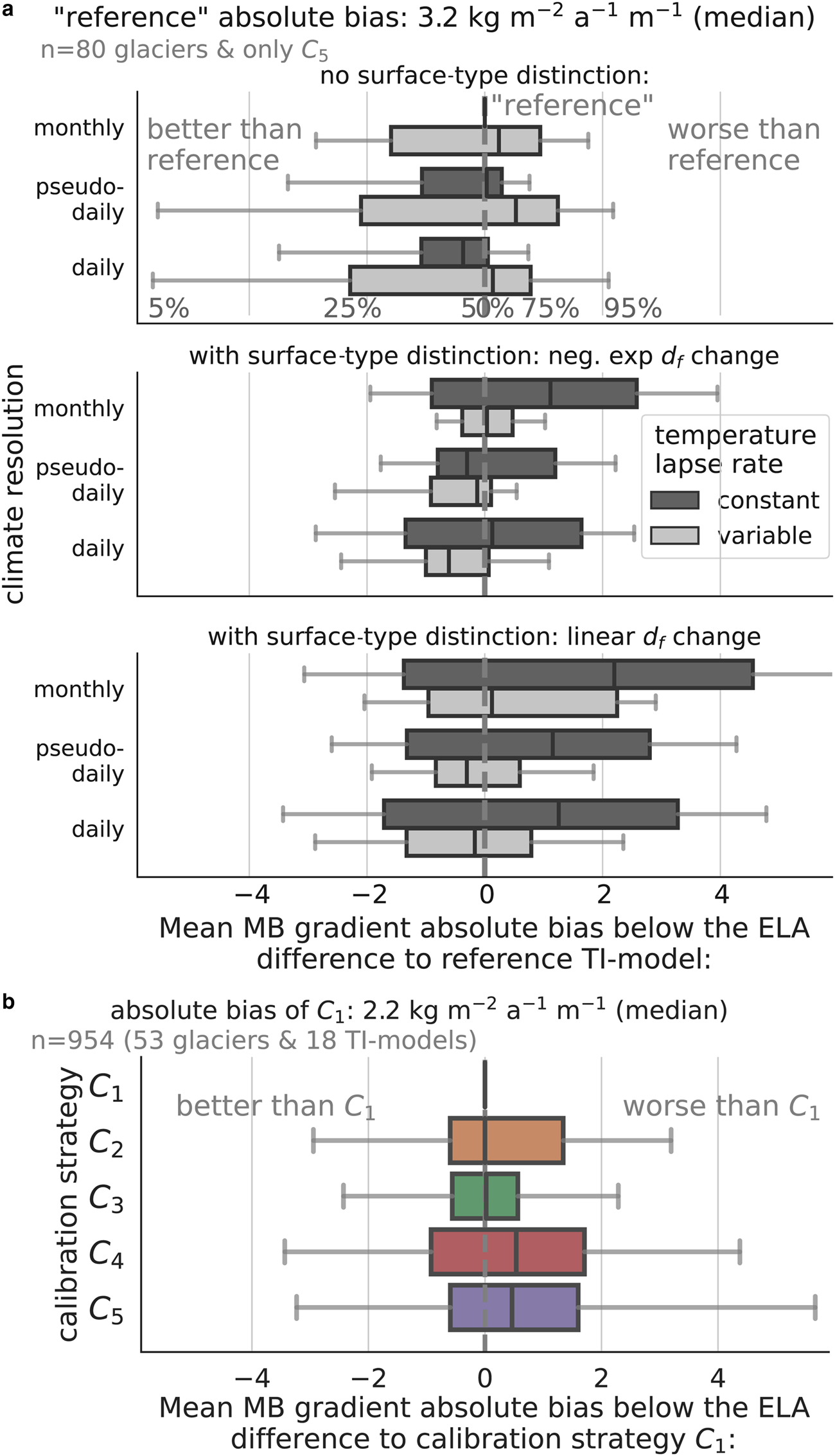
The modelled MB gradient below the ELA is larger when using a constant instead of a variable (mostly less negative) temperature lapse rate (Fig. S6a). The constant lapse rate choice aligns better with observed MB gradients below the ELA when no surface-type distinction is considered. However, it performs worse when surface-type distinction is applied (Fig. 3a). Including surface-type distinction increases the MB gradient (Fig. S6a) due to the creation of elevation-dependent degree-day factors (specifically in the “linear” case, Appendix, Fig. 8d). Therefore, using less negative (variable) temperature lapse rates together with surface-type dependent degree-day factors offset each other and result in a similar gradient and, thus, performance compared to the reference temperature-index model (Fig. 3a). No clear trend is observed in the MB gradient match below the ELA for different temporal climate resolution choices (Figs. 3a, S6a). However, when considering surface-type distinction and a less negative (variable) lapse rate, the pseudo-daily or daily choice better match the observed MB gradient below the ELA.
The temperature-index model performance based on the MB profile mean absolute error ratios are similar to those from the mean MB gradient absolute bias below the ELA (Fig. S7a). In contrast, the differences in how well the temperature-index model choices match the observed interannual MB variability are smaller (Figs. S6b, 7b). Nevertheless, the combinations that performed worse for the MB profile match (i.e. monthly, constant, with surface-type distinction) also performed worse in matching the annual MB variability (Figs. 3a, S7b).
3.2. Parameter choice and calibration strategy differences
3.2.1. Influence of equifinality on the temperature-index model output
Despite the simplicity of the temperature-index model, equifinality from model parameters strongly influences the MB variability, seasonality and gradient. We show these effects in Fig. 4 for a typical case of a large-scale glacier modelling study, where only one observation is available. Building upon Rounce and others (Reference Rounce, Hock and Shean2020a), we vary either the precipitation factor or temperature bias while always matching the geodetic MB and analysing corresponding changes in the modelled MB.
Influence of downscaling model parameters for the Hintereisferner glacier on the calibrated (a, b) degree-day factor (d f) to match the geodetic observations and on the resulting (c, d) interannual MB variability, (e, f) average winter MB and (g, h) mean elevation-dependent MB profiles (using the reference model option). Left plots (a, c, e, g) show varying precipitation factors (p f) with temperature bias (t b) set to zero, while right plots (b, d, f, h) show varying t b with p f set to two. Colourbar in (c–h) based on (a, b). std stands for standard deviation, mae for mean absolute error. Each d f, p f and t b combination matches the geodetic mean MB, and the combinations that best match in-situ observations are indicated. Figs. S9–S11 show the same for other glaciers.

Increasing the precipitation factor leads to a linear increase in the degree-day factor (Fig. 4a, Eq. (1)). More precipitation results in more solid precipitation and a higher winter MB (Fig. 4e), which is balanced by more melt to match the geodetic MB. The larger precipitation and degree-day factors also lead to a roughly linear increase in interannual MB variability (Fig. 4c), as the multiplicative parameters amplify precipitation and temperature anomalies; and cause more solid precipitation at the top and more melt at the bottom of the glacier, thus, a larger MB gradient (Fig. 4g).
Increasing the temperature bias while keeping the precipitation factor constant leads to a logarithmic decay of the degree-day factor (Fig. 4b). This is due to lower temperatures reducing the likelihood of crossing the melt threshold and increasing the likelihood of crossing the solid precipitation threshold (Eq. (1)). Lower temperature biases (and higher degree-day factors) logarithmically increase interannual MB variability (Fig. 4d). However, the influence on total variance is smaller than for precipitation factors (Fig. 4c), as the degree-day factor only affects the melt rates and the temperature bias has a limited impact on accumulation rates. Winter MB decreases only slightly with increasing temperature; an effect that becomes more substantial for larger temperature biases (Fig. 4f). Therefore, varying the temperature bias does little to improve the match with observed winter MB. Lastly, a positive temperature bias (and lower degree-day factor) decreases the MB gradient and leads to a more linear MB change with altitude (Fig. 4h) by balancing the reduction in solid precipitation at higher altitudes with less melt at lower altitudes.
3.2.2. Calibration strategy performance
Some calibration strategies use more data than others, enabling us to assess whether the additional calibration data improves the model performance (Figs. 3b, S6). We compare the MB profile match (i.e. the only validation data for C 1−5) of the calibration strategies relative to C 1 for all temperature-index model choices together and the 53 glaciers that could be calibrated and had observed MB profile data. Including more observational data for calibrating additional model parameters $(p_f \, \amp \, t_b)$ on a glacier-per-glacier level improves the match with the observed MB profile. Calibrating the degree-day factor and precipitation factor using the interannual MB variability (C 3) results in slightly better matched observed MB profiles compared to using mean winter MB observations (C 2). However, combining the interannual MB variability and mean winter MB for calibration (C 1) does not further improve the performance beyond matching the interannual MB variability alone (C 3).
4. Volume and runoff projections
The comparison to MB profiles in Section 3.1.3 showed minor differences in performance among temperature-index model choices, and only a few glaciers had additional data to calibrate all model parameters. Here, we evaluate how small changes in the model design of the temperature-index model and its calibration strategy affect glacier projections through 2100. To highlight differences we show results for a case study of Aletsch glacier, where differences are either from temperature-index model choices (only C 5, Fig. 5a) or calibration strategies (only reference model, Fig. 5b).
Aletsch glacier volume projections (2000–2100) for two SSP scenarios. We show the median, interquartile range (25%ile–75%ile, IQR) and total range resulting from (a) temperature-index (TI-) model choices using C 5 and (b) calibration strategies using the reference model. For this glacier, in (b), the calibrated parameters and thus projections for C 1, C 2 and C 5 are very similar. d f stands for degree-day factor, p f for precipitation factor and t b for temperature bias. We use the median volume from five GCMs. Fig. S12 shows the same for Hintereisferner glacier.

Additionally, from the 85 glaciers with in-situ observations, around 14% of their volume is projected to remain in 2060, relative to 2020, under the SSP1-2.6 scenario and 4% under SSP5-8.5, respectively. To avoid distortions caused by glaciers that completely disappear by 2100 regardless of temperature-index model choice or calibration strategy, we focus on a subset of non-vanishing glaciers for the subsequent comparisons (i.e. 45 out of 85 glaciers for SSP1-2.6 in Fig. 6, 15 glaciers for SSP5-8.5 in Fig. S13) and primarily discuss results for SSP1-2.6. Given the variety of temperature-index model choices and calibration strategies, the comparison of a given model choice (e.g. the variable versus constant lapse rate choice) is performed on all other temperature-index model combinations (e.g. the three climate resolution and three surface-type distinction choices) and all five calibration strategies together. Similarly, the comparison of a calibration strategy is estimated from all 18 temperature-index model choices. The inclusion of all combinations provides a more robust assessment of how a given option affects glacier projections regardless of other options. Differences are thus reported by dividing the individual glacier volumes for various temperature-index model choices against the reference model choice (e.g. constant lapse rate) or the glacier volume for the various calibration strategies against C 1. We repeat the same comparison for fixed-gauge glacier runoff projections (here the sum of melt and liquid precipitation components from the current and former glacierised areas, Figs. S16–S22), but also include the vanishing glaciers since the runoff accounts for the non-glaciated areas as the glaciers retreat.
(a) Individual glacier volume changes in 2040 and 2100 for 45 glaciers that could be calibrated on all options and still exist in 2100 under the SSP1-2.6 scenario. Individual glacier volume ratios for (b–f) temperature-index model choice and (g) calibration strategy. Distributions represented by the 5$\%_{\text {ile}}$ , 25$\%_{\text {ile}}$
 , 50$\%_{\text {ile}}$
 (median), 75$\%_{\text {ile}}$
 and the 95$\%_{\text {ile}}$
 . A rightward (leftward) distribution shift indicates larger (smaller) glacier volume compared to the reference option. (a) Volume changes are estimated from all 45 glaciers, 3 ⋅ 3 ⋅ 2 temperature-index model and 5 calibration options, volume ratios respectively by (b) 45 ⋅ (3 ⋅ 3) ⋅ 5, (c–f) 45 ⋅ (3 ⋅ 2) ⋅ 5 and (g) 45 ⋅ (3 ⋅ 3 ⋅ 2) glaciers and options. We use the median volume from five GCMs. See Fig. S13 for SSP5-8.5.

4.1. How do glacier projections from temperature-index model choices differ?
For Aletsch glacier, the temperature-index model choices result in differences in volume of up to 25% in 2100, relative to 2020, under SSP1-2.6 (Fig. 5a) and in glacier runoff of up to 40% (on one year, Fig. S16a). For glacier runoff, we found that the temperature-index model choices systematically influence projections on the considered glaciers (Fig. S22b–f). Using variable (less negative) lapse rates, daily climate resolution and no surface-type distinction often resulted in larger annual runoff. The impact of model choice on volume projections increases over time for SSP1-2.6 (Figs. 6b–f) as nonlinear feedbacks become more significant than the climate change signal, and the model choice influence on volume projections is analysed in the following.
4.1.1. Temperature lapse rate choice
The temperature lapse rate choice has the most systematic influence on volume projections with the variable (less negative) lapse rate having a median volume that is 19% (4–38%, representing 25th to 75th percentiles) smaller in 2100 under SSP1-2.6 compared to the constant choice (Fig. 6b, similar for SSP5-8.5 in Fig. S13b). As the glaciers retreat to higher elevations, the smaller calibrated degree-day factors (Fig. 1) do not compensate for the increasing impact of the less negative lapse rate resulting in more volume loss.
4.1.2. Temporal climate resolution choice
Using pseudo-daily or daily instead of monthly temperature data does not have a systematic effect on volume differences; however, the spread in projected volume differences is smaller when comparing the pseudo-daily versus monthly volume ratios (Figs. 6d,f). In the pseudo-daily choice, only the melt component differs from the monthly choice (if using the same precipitation factor), so melt increases if the influence of the monthly melt threshold is larger than the influence from the smaller calibrated degree-day factor applied in the pseudo-daily choice (Fig. 2) or vice-versa.
The melt component of the daily choice is likely influenced by an additional aspect, the changing daily temperature standard deviation with increasing temperatures. The possible reason is that GCMs predict decreasing standard deviations over time, which decrease the melt threshold influence and thus increase the influence of the likewise smaller calibrated degree-day factor (see Fig. S14 for details). Another difference in the daily choice is the daily liquid or solid precipitation. In a warmer climate, under the same precipitation, both winter accumulation and summer ablation might decrease for the daily temperature-index model due to decreased solid winter precipitation and a decreased melt threshold influence (also visible in the MB climate sensitivity analysis of Fig. 2a). In essence, projected differences between daily and monthly choices depend on how the balance shifts between the calibrated parameter differences and the influence of thresholds for melt and solid precipitation.
4.1.3. Surface-type distinction choice
Using a surface-type dependent degree-day factor instead of a constant degree-day factor results in a minimally smaller projected glacier volume in 2040, while for many glaciers, it results in a relatively larger glacier in 2100 under SSP1-2.6 (Figs. 6c,e). However, under SSP5-8.5, applying surface-type distinction results in a smaller glacier in 2040 and 2100 compared to no surface-type distinction (Figs. S13c,e). Under SSP5-8.5 and the first two decades of SSP1-2.6 after 2020, the differences from the surface-type distinction is likely a result of the glaciers’ increased relative ice-covered ablation area having a more critical role in future specific MB than during the calibration period. Thus, the CPDD are greater than in the calibration period, which results, as shown in the temperature sensitivity analysis of Fig. 2c, in higher negative specific MB anomalies when including surface-type distinction due to the higher ice degree-day factor (Fig. 1). However, in the last decades of SSP1-2.6, many glaciers are projected to retreat enough to get into a quasi-equilibrium state or even advance slightly because of local cooling (e.g. Aletsch glacier in Fig. 5a). This effect cannot be explained by the fixed-geometry temperature sensitivity experiment (Fig. 2). Only when considering the glacier retreat the accumulation area ratio increases so that the smaller snow degree-day factor becomes more important than in the calibration period and thus explains the larger glacier.
4.2. How do glacier projections from the calibration strategies differ?
In the first three decades after 2020, the five calibration strategies influence the Aletsch glacier volume projections more than the temperature-index model choice (Fig. 5). For that glacier, a larger precipitation factor or negative temperature bias led to faster projected volume loss in the first three decades after 2020 but less volume loss by the end of the century under SSP1-2.6 (Figs. 7a,b). As the glacier retreats, the increased solid precipitation (precipitation- or temperature-induced) at higher altitudes outweighs the larger degree-day factor.
Influence of equifinality on (a, b) volume and (c, d) runoff projections for the Aletsch glacier under SSP1-2.6. The colours indicate the precipitation factor (p f) or temperature bias (t b) as presented in (e, f), which shows the relation between p f or t b and average annual runoff. For each p f or t b, a degree-day factor was calibrated to match the same average geodetic MB. On the left, (a, c, e), t b is set to zero and p f is varied while on the right, (b, d, f), p f is set to 2 and t b is varied. Projections are median estimates from five GCMs using the reference model. The four runoff components are in Fig. S20. Fig. S21 shows the same for Hintereisferner glacier.

For all non-vanishing analysed glaciers (Fig. 6g), the different calibration strategies result in similar projected individual glacier volumes in 2040, but their estimates diverge in 2100. With additional glacier-specific data, such as using the average winter MB or standard deviation of the annual MB to calibrate the temperature-index model parameters (i.e. done in C 1, C 2, C 3), slightly more glacier volume is projected to be lost under SSP1-2.6. This effect gets stronger under SSP5-8.5 for the 15 remaining glaciers (Fig. S13g). However, the calibration strategy's influence on the glacier projections depends strongly on the individual glacier. This variability can be partly attributed to the equifinality (i.e. the influence of choosing a relatively larger precipitation and degree-day factor, Fig. 7) and partly to the fact that some glaciers are more in an ablation- or accumulation-dominant situation.
We also assess whether one calibration strategy results in more or less spread between the different temperature-index model choices (Fig. S15). To compare this, we use the standard deviation of the temperature-index model choice volume ratio distribution of any variant versus the reference model. Generally, using more data for calibration and allowing for glacier-specific model parameters (i.e. C 1) creates a more extensive spread between temperature-index model choices with the standard deviation being almost twice as large in C 1 compared to C 4 (strategy where only the degree-day factor changes between glaciers). Allowing the precipitation factor to vary on a glacier-per-glacier scale (all strategies except C 4), as well as the temperature bias (only C 1), might explain the greater temperature-index model variability during non-calibrated periods.
We found a strong increase in annual glacier runoff for larger precipitation factors, while the temperature bias choice had minimal non-systematic influence (exemplarily shown in Figs. 7c–f). A larger precipitation factor directly increases liquid precipitation, indirectly increases melt runoff components due to a larger calibrated degree-day factor and increases annual runoff variance (Figs. 4a, S20). If different precipitation factors are used, glacier runoff varies strongly between the calibration strategies and is smallest for the strategy with the overall smallest precipitation factor (i.e. C 4 in Fig. S22g for 85 examined glaciers). How and if total runoff is influenced by the temperature bias depends on the runoff components allocation and their temperature influence. For Aletsch glacier, the runoff components offset each other throughout the entire period (Figs. 7d,f).
5. Discussion
5.1. Model performance and climate sensitivity differences
Our study showed that different temperature-index model choices and calibration strategies can result in considerable differences in modelled interannual, seasonal and elevation-dependent MB, even over the calibration period with fixed glacier geometry. Here we discuss how our findings compare to other studies by examining the temperature-index model parameter choice and equifinality (Section 5.1.1), the sensitivity of different MB models (hereon using MB models when including non-temperature-index models) to the climate (Section 5.1.2), whether more complex MB models improve projections (Section 5.1.3) and the added value of more observations (Section 5.1.4).
5.1.1. Temperature-index model parameter choice and equifinality
The range of the degree-day factor of ice in this study (for model choices with surface-type distinction) is within the range of other regional temperature-index models (e.g. Huss and Hock, Reference Huss and Hock2015; Rounce and others, Reference Rounce2020b). Our average precipitation factor, considering all model and calibration options, is around three, which is up to two times higher than in previous studies (e.g. in Huss and Hock, Reference Huss and Hock2015; Rounce and others, Reference Rounce2020b). The higher precipitation factor is most likely due to differences in the climate datasets, investigated glaciers, precipitation gradients and calibration strategies. For example, Huss and Hock (Reference Huss and Hock2015) and Zekollari and others (Reference Zekollari, Huss and Farinotti2019) restrict the precipitation factor to a maximum value of two and then change the degree-day factor or temperature bias accordingly to match observations. The equifinality issue further complicates comparisons, as higher degree-day factors can be balanced by larger precipitation factors or lower temperature biases (Fig. 4, also discussed in Rounce and others, Reference Rounce2020b).
5.1.2. MB model climate sensitivity differences
We compare our climate sensitivities (Fig. 2) to similar experiments by Bolibar and others (Reference Bolibar, Rabatel, Gouttevin, Zekollari and Galiez2022, all 660 French Alpine glaciers; in the following BO22) and Vincent and Thibert (Reference Vincent and Thibert2023, 2 Alpine glaciers; in the following VT23). BO22 compare a deep-learning MB model with daily temperature, precipitation, snowfall and glacier topography as input to model annual MB to a linear LASSO (a regularised multi-linear regression) model. Their deep-learning model outperformed the LASSO model, particularly for extreme MB, but their LASSO model behaves differently than a temperature-index model, justifying further study.
Without surface-type dependent degree-day factor change, our models respond to CPDD anomalies in a similar fashion as BO22's LASSO model. We found nonlinear MB responses to CPDD anomalies when including surface-type distinction (Fig. 2b), consistent with VT23. The BO22 deep-learning MB model captured a similar but less pronounced nonlinearity. This can be partly explained by increased ice surface fractions and, thus, temperature sensitivities for large positive CPDD anomalies. The lesser nonlinearity in BO22 suggests that counteracting processes, such as reduced solar radiation impact, may affect MB sensitivity to rising temperatures. Surface-type distinctions were not explicitly modelled in BO22, and only CPDD anomalies during the ablation season were considered.
We found driver-dependent specific MB sensitivities for winter and summer solid precipitation anomalies. If induced by temperature changes, solid winter or summer precipitation anomalies create nonlinearities in MB sensitivity, either increasing or decreasing, across all our temperature-index model choices (Fig. 2), aligned with VT23. In contrast, BO22 directly incorporated solid precipitation anomalies as predictors in their models, making them independent of temperature changes or respective solid total precipitation anomalies. Our precipitation-induced solid precipitation anomaly resembles the approach in BO22, although in our case, solid winter and summer precipitation linearly correlate by the applied precipitation factor that modifies annual precipitation. Similar to our temperature-index models without surface-type distinction, the BO22 LASSO MB model resulted in a linear relation between precipitation-induced solid precipitation and MB. However, unlike all our temperature-index model choices, the BO22 deep-learning MB model has a larger MB sensitivity for small solid precipitation anomalies and a smaller MB sensitivity for strong positive and negative anomalies, specifically for solid summer precipitation anomalies.
Comparing the studies is complex. Although BO22 applied solid precipitation anomalies independent of other variables, their deep learning MB model was trained using data where positive solid summer precipitation anomalies were associated with negative temperature anomalies in the historical climate, for example. The decreasing MB sensitivity for positive solid summer precipitation anomalies in BO22 was also observed in all our temperature-index model choices if applying a temperature-induced solid summer precipitation anomaly. However, the opposing nonlinear sensitivities for negative anomalies still require an explanation. BO22 argue that their deep-learning MB model may capture decreasing ice degree-day factors for increasing temperatures (Braithwaite, Reference Braithwaite1995; Huss and others, Reference Huss, Funk and Ohmura2009), which can be attributed to changing relationships between melt and temperature driven by longwave radiation and turbulent fluxes, despite unchanged shortwave radiation fluxes (Gabbi and others, Reference Gabbi, Carenzo, Pellicciotti, Bauder and Funk2014; Ismail and others, Reference Ismail, Bogacki, Disse, Schäfer and Kirschbauer2023).
Finally, the rest of our study demonstrates that the results of such idealised sensitivity experiments, where the effects of equifinality and the feedbacks with changing glacier geometries are ignored, should be interpreted with caution.
5.1.3. MB model performance comparisons
Our goal was to determine the best temperature-index model choice for a calibration strategy where only geodetic glacier observations are used (C 5). While different temperature-index model combinations can perform similarly as different effects balance one another, using daily data, variable (less negative) lapse rates and a varying neg. exp. degree-day factor is arguably the most realistic physically and matches the MB profile best (Fig. 3a). Furthermore, this combination resulted in the third-highest amount of non-failing glaciers during calibration (235 of 247, Fig. S5b). To our knowledge, no other study compared the differences in performance between our temperature-index model choices. However, some studies have compared the performance of temperature-index models to enhanced models incorporating a separate shortwave radiation term. These enhanced models have shown improved performance by reducing the sensitivity to temperature changes (Gabbi and others, Reference Gabbi, Carenzo, Pellicciotti, Bauder and Funk2014), although another study found no difference in performance over short time periods (Réveillet and others, Reference Réveillet, Vincent, Six and Rabatel2017). In a regional-scale study, Huss and Hock (Reference Huss and Hock2015) did not observe any added value in model performance when using a simplified energy-balance model by Oerlemans (Reference Oerlemans2001). The scarcity of calibration data makes it challenging to assess the added value of model complexity at large scales. More complex models often require more glacier-specific parameters, and fixing these parameters globally may overshadow uncertainties originating from equifinality.
5.1.4. Added value of more observations for the calibration
We found a slightly improved temperature-index model performance for calibration strategies using in-situ observational data, specifically when using the interannual MB variability to calibrate the precipitation factor for every glacier (Figs. 3b, S8). Other studies comparing the added value of more observations at smaller scales are discussed in the supplementary material (Section S4.1). In the future, new remote sensing data and methods estimating the MB gradient or even seasonal and interannual MB may improve model performance and reduce equifinality uncertainties at regional to global scales. Interferometric swath altimetry applied on CryoSat-2 produces glacier thinning estimates at monthly temporal resolution (Jakob and others, Reference Jakob, Gourmelen, Ewart and Plummer2021), yet at coarse spatial resolution (100 × 100 km bins) and decadal estimates at a higher resolution of 500 m (Jakob and Gourmelen, Reference Jakob and Gourmelen2023). By combining glacier thinning with surface velocity observations and ice thickness estimates, altitudinally-resolved specific mass balances can be derived (Miles and others, Reference Miles2021). Those are however still uncertain, specifically over the accumulation area when the necessary remote sensing products are less accurate (e.g. ice velocity). Additionally, these new techniques and datasets are not yet globally available and require a density assumption to convert elevation to mass change, introducing further uncertainties (Huss, Reference Huss2013). A potential solution to address this is to apply a firn densification model. Hence, glacier models combined with remote sensing could even help detect forcing biases (e.g. Guidicelli and others, Reference Guidicelli, Huss, Gabella and Salzmann2023). Using higher-resolved dynamically downscaled climate data could also constrain local downscaling parameter ranges (e.g. Karger and others, Reference Karger2017). It is however unlikely that large-scale studies will benefit from drastically improved forcing data in the near future.
Without this additional data, we favour calibration strategy C 5 over C 4 for OGGM users. Using glacier-specific precipitation factors depending on the glaciers’ average winter precipitation (C 5) instead of the same precipitation factor for every glacier (C 4) results in a less wide distribution, i.e., unrealistically large precipitation values are avoided. In C 5, we use the logarithmic relation between winter precipitation and calibrated precipitation factor of C 2, where winter MB (i.e. very precipitation-factor dependent) is matched. Thus another reason to use C 5 is that the precipitation factor dependence on the winter precipitation could make physically more sense and is independent of the temperature-index model choice.
5.2. Volume and runoff projection differences
We project that Aletsch glacier, the largest glacier in the European Alps, will lose 50–83$\%$ of its volume under SSP1-2.6, and $> 95\%$
 under SSP5-8.5, relative to 2020, for the different temperature-index model and calibration options of this study (Fig. 5). Aletsch glacier projections with a full-stokes glacier model (Jouvet and Huss, Reference Jouvet and Huss2019) and two dynamical large-scale glacier model studies (Zekollari and others, Reference Zekollari, Huss and Farinotti2019; Rounce and others, Reference Rounce2023) under approximately the same climate scenarios lie at the lower part of our loss ranges. The reasons for these differences are difficult to disentangle. Below, we compare our glacier projection differences to previous studies in regard to the MB model choice (Section 5.2.1), the equifinality and calibration strategy (Section 5.2.2), and generally to the findings of GlacierMIP2 and Rounce and others (Reference Rounce2023) (Section 5.2.3).
5.2.1. MB model influence on glacier projections
In a warming climate, less negative temperature lapse rates result in more projected glacier loss and larger runoff (Figs. 6, S22). How different our lapse rates are from other large-scale glacier studies is unknown. It also needs to be clarified how well the ERA5-derived free-atmosphere temperature lapse rates used here and in these studies are related to the true near-surface temperature lapse rates. Some studies suggest that near glacier-surface lapse rates are weaker during the ablation season compared to free-atmosphere estimates (e.g. Gardner and others, Reference Gardner2009; Hodgkins and others, Reference Hodgkins, Carr, Pálsson, Guðmundsson and Björnsson2013). Our ERA5-derived estimates are, however, stronger (more negative) in the ablation compared to the accumulation season (not shown).
Interestingly, the temporal climate resolution choice has no systematic influence on regional glacier change projections (Fig. 6). Using pseudo-daily climate with no future changes in the daily temperature standard deviation, i.e., as applied in Huss and Hock (Reference Huss and Hock2015) and Zekollari and others (Reference Zekollari, Huss and Farinotti2019), results only in minor projection differences compared to the monthly choice. The influence of using daily instead of monthly data depends on how the balance shifts between calibrated parameter differences and the impact of thresholds for melt and solid precipitation. We found larger runoff with daily data, which is relevant because this choice is beneficial when coupling glacier models with hydrological models to get daily runoff.
The volume response of temperature-index models with and without surface-type distinction (Figs. 6, S13) depends on the future glacier state, while runoff is smallest without surface-type distinction (Figs. S22c, e). If the future accumulation area ratio is smaller than during the calibration period, temperature-index models with surface-type distinction cause more mass loss (more melt over ice), and vice versa. Other studies did not analyse the influence of small temperature-index model changes as we did in our study, especially not on runoff. When comparing their temperature-index model to a simplified energy-balance model, Huss and Hock (Reference Huss and Hock2015) found that the energy-balance model reduced glacier loss projections by about 20%, which is similar to the projection differences resulting from our temperature lapse rate choices.
5.2.2. Calibration strategy and equifinality influence on glacier projections
We found slightly more glacier volume loss when calibrating glaciers with additional in-situ observations (Fig. 6), but differences varied for individual glaciers due to, e.g. the temperature-index model parameter choice (exemplarily shown in Figs. 7a,b) or the accumulation-area ratio relative to the calibration period. These differences highlight the influence of equifinality on glacier volume projections, as all options matched the geodetic observation. Huss and Hock (Reference Huss and Hock2015) found that equifinality influenced glacier projections of selected regions by $\pm 18\%$ compared to their reference calibration strategy (assessed by 16 fixed parameter combinations). Compagno and others (Reference Compagno, Zekollari, Huss and Farinotti2021) analysed the influence of small precipitation factor range shifts (±0.6) in their three-step calibration and found glacier projection differences of ≤4%. Larger precipitation factor ranges and a different order in their three-step calibration could result in more significant differences. Rounce and others (Reference Rounce2020b) found that glacier volume projections can be greatly affected by equifinality at the glacier scale, but regionally, the GCM choice is more important. However, this influence may depend on how uncertainties are aggregated between glaciers (independent or correlated).
In accordance with Rounce and others (Reference Rounce2020b), we noted that glacier runoff projections are more influenced by the choice of temperature-index model parameters than volume projections. Larger precipitation factors led to increased annual glacier runoff, while the temperature bias had no systematic influence (Fig. 7, Fig. S22g C 4). These findings do not contradict studies suggesting that interannual precipitation influences glacier runoff less than temperature changes (e.g. Pramanik and others, Reference Pramanik, van Pelt, Kohler and Schuler2018; Banerjee and others, Reference Banerjee, Singh and Sheth2022), as we vary the precipitation factor or temperature bias before the calibration, which also changes the degree-day factor and, thus, the melt on glacier runoff components (Figs. S20a,b).
5.2.3. Comparison to GlacierMIP2 and Rounce and others (2023)
The sources of projection differences between studies and within GlacierMIP2 (Marzeion and others, Reference Marzeion2020) are difficult to disentangle as not only the MB model or the calibration strategy but also, e.g. the climate data, its bias correction and the initial state can be different between glacier models.
GlacierMIP2 compared projections of different large-scale glacier models in a coordinated effort. The study also estimated each model's sensitivity of the mean specific mass balance to temperature changes using an inverse approach which we repeated with our temperature-index model variants. We found weaker temperature sensitivity without surface-type distinction compared to the linear changing choice (on average 34% weaker) or when using daily instead of monthly data (18% weaker). To a similar magnitude, from the four near-global models using temperature-index models in GlacierMIP2 (their Fig. 8b), those without surface-type distinction (Marzeion and Hofer, Reference Marzeion, Jarosch and Hofer2012; Maussion and others, Reference Maussion2019) had a weaker temperature sensitivity than those with surface-type distinction (Radić and others, Reference Radić2014; Huss and Hock, Reference Huss and Hock2015). However, besides the MB model choices analysed in our study, the applied local-scale climate, dependent on, e.g., the chosen climate datasets, precipitation factors or gradients, also influences the temperature sensitivity differences. In GlacierMIP2, one of the two energy-balance models had the weakest temperature sensitivity and the two energy-balance models generally projected the least negative mass balances. The reason may be a temperature-oversensitivity of temperature-index models due to relatively small future changes in downwelling long- and short-wave radiation despite increasing temperatures (Shannon and Others, Reference Shannon2019).
The model used to create projections for Rounce and others (Reference Rounce2023) is most similar to OGGM as it uses the glacier dynamics module of OGGM, but the MB module of the Python Glacier Evolution Model (PyGEM). They project in 2100 around 16% lower relative glacier volume than our median projections under SSP1-2.6 (for all model options, three common GCMs, and 41 non-vanishing glaciers). The differences are reduced on median to 2–15% lower relative glacier volumes (calibration-strategy dependent) when comparing only to our temperature-index model that resembles most to their model (i.e. variable lapse rates, neg. exp. degree-day factor change and pseudo-daily climate). Specifically, applying the same temperature lapse rate choice reduced the volume projection differences. Their runoff projections are generally smaller, hinting at smaller precipitation factors.
5.3. Limitations
Due to the lack of robust, high temporally and spatially resolved observational data, we only analysed 88 glaciers, of which most come from the northern mid-latitudes (28 from Central Europe and 19 from Scandinavia). Around half of these glaciers will vanish by 2100 for at least one of the options, even under SSP1-2.6. The examined sample may thus not represent the response of global glacier change. In addition, some glaciers could not be calibrated with the proposed calibration strategies and model parameter ranges, hinting at missing model physics, poorly downscaled local climate or observational errors. We only used in-situ and 20-year average geodetic MB observations and neglected their own uncertainties. The uncertainties from observations and equifinality could be incorporated using Bayesian inference (Rounce and others, Reference Rounce2020b), but it remains challenging to aggregate and disentangle these uncertainties from individual to regional scales. Per design, we also did not assess the influence of uncertainties from GCMs, initial state and bias correction and just focussed on the temperature-index model choice and calibration strategy.
Since small changes in the temperature-index model had such a large influence, we did not implement further MB models, which could be the next step. However, even simple choices, such as how the degree-day factor gradually changes with ageing snow, still need to be determined. We propose two approximations and favour the negative exponential degree-day factor change choice over the linear choice. We could also have applied simpler surface-type distinction methods with a step-wise change between snow, firn and ice (e.g. Huss and Hock, Reference Huss and Hock2015; Rounce and others, Reference Rounce, Hock and Shean2020a). We chose the monthly ageing snow ageing bucket system (see Section A.1), as it has the potential to estimate firn densification and may allow calibration on more reliable elevation changes. We did not explicitly include refreezing, as large-scale observations, e.g. englacial temperature, are missing, nor did we include debris cover.
We vary three model parameters and keep them constant over time, although, e.g. the snow degree-day factor was found to vary specifically under clear-sky conditions (e.g. depending on altitude and solar inclination, Ismail and others, Reference Ismail, Bogacki, Disse, Schäfer and Kirschbauer2023). The influence of using daily or monthly climate data could equally depend on the chosen solid precipitation and melt thresholds which we fixed globally. For example, Matthews and Hodgkins (Reference Matthews and Hodgkins2016) found that tuning the melt threshold increased their skill and resulted in a stationary degree-day factor over a 34-year study period on an Icelandic glacier for a snow/firn-covered location. Moreover, we found that the temperature lapse rate choice strongly influenced the MB, but we assumed constant lapse rates over the years. Neglecting potential future enhanced warming rates with elevation (Pepin and others, Reference Pepin2015; Palazzi and others, Reference Palazzi, Mortarini, Terzago and von Hardenberg2019) could underestimate glacier mass loss.
Glacier hypsometry changes were not considered in the climate sensitivity analysis (Sections 3.1.2, 5.1.2), which created differences to our dynamical projections where glaciers adapt to the changing climate. The calibration over 20 years neglects ice dynamics and assumes constant glacier area, leading to potential mass change overestimates, particularly for glaciers with higher mass flux rates (Mukherjee and others, Reference Mukherjee2022).
6. Conclusions
Our findings reveal that model design options, often assumed to be small (e.g. variations of temperature-index model and calibration options), can influence MB model performance as well as volume and runoff projections. By systematically changing one model option at a time within the OGGM framework, we provide insight into glacier model behaviour differences that are impossible to unveil from large-scale glacier model intercomparison projects.
Due to equifinality, even the simplest temperature-index model responded differently to different combinations of parameters. For example, we found increasing interannual MB variability, winter MB and MB elevation gradients for increasing precipitation factors and decreasing temperature biases. To assess the added value of a given process and, simultaneously, of better-resolved MB observations, we focussed on 88 glaciers with available in-situ observations. While specifically using the interannual MB variability to calibrate otherwise fixed parameters led to better MB model performance, the added value of additional MB complexity is challenging to demonstrate. Nevertheless, the most physically realistic temperature-index model choice (i.e. including surface-type distinction with a negative exponential degree-day factor change, variable lapse rates and daily data) performed better than others. Matching approximately the observed MB gradient is essential due to its direct influence on the ice flux and ice dynamics (e.g. Maussion and others, Reference Maussion2019). In the absence of additional calibration data, selecting the precipitation factor based on a glacier's winter precipitation may be more physically meaningful than using a globally fixed value, although we did not find improved model performance for this calibration strategy.
We find strong nonlinearities and counter balancing effects of the model choice, which depend on the differences between the future glacier state and climate compared to the calibration period. These patterns were consistent across various calibration and other temperature-index model options; thus, the projection differences between temperature-index models were also a result of their design differences and did not solely stem from equifinality. In a warmer climate, less negative temperature lapse rates result in systematically smaller glaciers by 2100. Using monthly-changing snow-age dependent degree-day factors produced more or less glacier loss depending on whether the glacier accumulation area ratio is smaller or larger compared to the calibration period, respectively. More calibration data generally resulted in smaller projected glacier volumes, but the influence varied at the individual glacier scale, highlighting uncertainties related to equifinality.
Comparisons between options were difficult, as we projected that half of the examined glaciers with in-situ data will lose 50% of their volume by 2039, relative to 2020, independent of the climate scenario. As we showed that additional observations have the potential to reduce projection uncertainties, it is necessary to search for more climate-resilient glaciers to continue long-term in-situ observations. While the models and calibration strategies used in previous model intercomparisons (e.g. GlacierMIP2) differed much more than our model options, we found that even small changes can substantially influence individual glacier projections. That influence can increase over time and become even more important when considering critical variables such as glacier runoff.
Supplementary material
The supplementary material for this article can be found at https://doi.org/10.1017/aog.2023.57.
Data
The code to create the figures is publicly available in the Github repository https://github.com/lilianschuster/oggm_mb_sandbox_option_intercomparison that used the OGGM massbalance-sandbox repository (https://github.com/OGGM/massbalance-sandbox). The projections and other data are publicly available via Zenodo: https://doi.org/10.5281/zenodo.7660887.
Acknowledgements
The authors would like to thank Jordi Bolibar for the useful discussions on the MB model climate sensitivities (Sections 3.1.2, 5.1.2), and the two anonymous reviewers for their constructive, detailed and helpful comments which helped to improve the overall quality and clarity of the paper. Lilian Schuster is recipient of a DOC Fellowship of the Austrian Academy of Sciences at the Department of Atmospheric and Cryospheric Sciences, University of Innsbruck (No. 25928). She has also been funded by University of Innsbruck's “Exzellenzstipendien für Doktoratskollegs” fellowship programme. This project has received additional funding from the European Union's Horizon 2020 research and innovation programme under grant agreement No. 101003687. This text reflects only the author's view and that the Agency is not responsible for any use that may be made of the information it contains. This project was also supported by NASA under grant Nos. 80NSSC20K1296 and 80NSSC20K1595.
A. Appendix
A.1 Snow ageing bucket system
We differentiate between snow, various firn age stages and ice by applying a monthly ageing update. At initialisation, we assume to have ice everywhere. Then, for each month, solid precipitation that has not melted in that same month goes inside the snow bucket. When melting occurs, the youngest bucket, the snow bucket, is emptied first. If this is or gets empty, the next older bucket is emptied and so on. The ageing update of the remaining snow occurs at the end of each month. The snow amount (in kg m−2) that did not melt over that month is transferred to the next older bucket, which is the one-month-old bucket. The same is repeated for all other buckets. If snow has fallen six years ago and has not melted, i.e., it was transferred each month to the next older bucket, it will be finally converted to ice. There is no ice bucket, as OGGM does the MB calibration before the ice thickness inversion (at this stage, OGGM does not know how much ice lies below the surface). Thus, the mass is just removed from the buckets, and the gridpoint is treated as ice if all buckets are empty. We use six years of spinup to initialise the buckets. Note that we neglect ice dynamics in this approach. The monthly ageing update choice with monthly buckets is much more computationally expensive than a yearly ageing update (implemented but not used). However, the monthly ageing update choice is more realistic as the degree-day factor (i.e. depending on the surface type) varies strongly between the seasons. With this bucket system, we do now have the possibility to track for each month how much snow or firn amount (in kg m−2) there is for each bucket and each height-gridpoint along the flowline, i.e., we can track the snow age in the vertical column in a monthly resolution.
Using a monthly resolution, we can visualise the yearly cycle of surface-type distinction for a single exemplary year (here the Hintereisferner glacier, Appendix Fig. 8). At the end of October, at the upper part of the glacier, relatively fresh snow is above the older firn layers and the actual glacier ice. In the lower part, very little fresh snow or even no snow is above the glacier (Appendix Fig. 8a). After the winter, here in May, the fresh snow is distributed equally over the glacier. However, at the lowest part, winter snow starts to melt away (Appendix Fig. 8b). In August, only ice is left on the entire lower part of the glacier, and at the upper part, winter snow and even some of the firn layers are melting away (Appendix Fig. 8c). Thus, this method is a new way to distinguish between snow, firn and ice surfaces which can be used to apply surface-type dependent degree-day factors or for potential future other applications (e.g. estimating snow densities). In the neg. exp. case, the degree-day factor is larger for snow that is a few months old up to a few years old firn, due to the faster initial change (Appendix, Fig. 8d). This faster change is offset by a lower degree-day factor for ice and very fresh snow.
Snow age tracking with snow buckets depicted for the Hintereisferner glacier for end of (a) October 2008, (b) May 2009 and (c) August 2009. The approximate area-weighted mean altitude of that glacier is shown. Snow is considered ice after 72 months without melting. In (a, b, c), the amount of ice is not shown. In (d), the calibrated evolution of the snow to ice d f is illustrated for different assumptions of degree-day factor (d f) change with snow age. In (e), the resulting average altitudinal-dependent MB over 2000–2019 is shown for the different choices together with the observations. In (f, g), only the melt MB profile is shown for October 2008 and May 2009. With surface-type distinction, (f) more melt occurs in summer and (g) less in winter compared to no surface-type distinction due to the applied snow-to-ice gradient of d f (specifically at lower altitudes). We show here calibration strategy C 5 with resulting precipitation factor (p f) of 3.45 for the temperature-index model with variable temperature lapse rates and daily climate data.


 Open access