


1. Introduction
The surface fluxes over sea ice influence the mass balance and drift direction of sea ice (e.g. Vihma and others, Reference Vihma, Johansson and Launiainen2009). Such studies in Polar Regions have been attracting great attention, due to its strong effect to the regional and global climate (e.g. King and others, Reference King, Anderson, Smith and Mobbs1996, Reference King, Connolley and Derbyshire2001; Reijmer and others, Reference Reijmer, Meijgaard and Van den Broeke2003; Bourassa and others, Reference Bourassa2013). However, very limited observations of radiative and turbulent characteristics have been performed over the Antarctic sea ice (e.g. Vihma and others, Reference Vihma, Johansson and Launiainen2009; Weiss and others, Reference Weiss, King, Lachlan-Cope and Ladkin2011; Yu and others, Reference Yu2019), while most in situ studies of surface radiation and turbulent fluxes in Polar seas have been carried out in the Arctic to date (e.g. Perovich and others, Reference Perovich, Grenfell, Light and Hobbs2002; Schrӧder and others, Reference Schröder, Vihma, Kerber and Brümmer2003; Grachev and others, Reference Grachev, Andreas, Fairall, Guest and Persson2007; Perovich and Polashenski, Reference Perovich and Polashensk2012; Walden and others, Reference Walden, Hudson, Cohen, Murphy and Granskog2017). Furthermore, most existing observational records over the Antarctic sea ice are either too short or do not involve all surface energy budget components. With these limited observations, the sea-ice conditions around Antarctica were found to be quite different from the Arctic (Wendler and others, Reference Wendler, Moore, Dissing and Kelley2000).
To find the mechanism controlling the variation of sea-ice thickness in the Antarctic region, a proper estimation of surface heat fluxes over sea ice was crucial (Vihma and others, Reference Vihma, Johansson and Launiainen2009; Lazzara and others, Reference Lazzara, Weidner, Keller, Thom and Cassan2012). Because of the rareness of directly turbulent observation, surface energy budget over sea ice in the Antarctic region was studied mainly by using numerical models (Andreas and others, Reference Andreas, Tucker and Ackley1984; Andreas, Reference Andreas1987; Stearns and Weidner, Reference Stearns and Weidner1993; King and others, Reference King, Anderson, Smith and Mobbs1996, Reference King, Connolley and Derbyshire2001). Previous studies show that Monin-Obukhov similarity theory (MOST) is applicable from unstable to stable conditions in Polar Regions (e.g. Garratt, Reference Garratt1992; Rodrigo and Anderson, Reference Rodrigo and Anderson2013; Liu and others, Reference Liu2019), although some limitations exist when the gradient Richardson number is larger than ~0.2–0.25 (Grachev and others, Reference Grachev, Andreas, Fairall, Guest and Persson2013). Before using these MOST-based models to estimate surface turbulent fluxes over sea ice, the real surface energy budget status as well as some crucial parameters, such as roughness lengths, must be ascertained or verified from observation (Munro, Reference Munro1989; King and others, Reference King1990; Yagüe and Cano, Reference Yagüe and Cano1994; Cassano and others, Reference Cassano, Parish and King2001; Cullen and others, Reference Cullen, Mölg, Kaser, Steffen and Hardy2007; Vignon and others, Reference Vignon2017).
Previous studies have found that roughness lengths over ice surface are ~10−5~10−2 m, which are affected by the local morphology, melting and snowdrifting (King and Anderson, Reference King and Anderson1994; Bintanja and Van den Broeke, Reference Bintanja and Van den Broeke1995; Van den Broeke and others, Reference Van den Broeke, van As, Reijmer and van de Wal2005; Guo and others, Reference Guo2011). Based on the laboratory and field data, Andreas (Reference Andreas1987) proposed a surface-renewal model to relate the aerodynamic roughness length (z 0m) and the scalar roughness length for temperature (z 0h) over snow and ice surface, and the model was further modified by Smeets and Van den Broeke (Reference Smeets and Van den Broeke2008b) over a rougher surface. In the surface-renewal model, kB −1 [≡ log(z 0m/z 0h)] was parameterized with friction velocity (u *) and z 0m. Nevertheless, studies show that, over vegetated land surface, thermal conditions also impact kB −1 and lead to a diurnal variation (e.g. Sun, Reference Sun1999; Rigden and others, Reference Rigden, Li and Salvucci2018), while Yang and others (Reference Yang, Koike, Fujii, Tamagawa and Hirose2002 and Reference Yang2007) proposed a temperature scale (T *) dependent model to calculate kB −1 over the surface covered by bare soil or partially covered by very short vegetation. On the other hand, Brunke and others (Reference Brunke, Zhou, Zeng and Andreas2006) indicated that there was no evident dependence of z 0h on surface temperature or friction velocity and suggested a constant z 0h of 5 × 10⁻⁴ m for sea-ice surface in the Arctic region. It is obvious that the parameterization for z 0h remains unsolved owing to natural complexities of air–sea-ice surface interaction in the Antarctic region.
This paper concentrates on the evolution of surface energy components and the parameterization of roughness lengths by using the data collected at an Antarctic sea ice station from 8 April 2016 through 26 November 2016. To our best knowledge, this observation is the longest direct measurement of latent heat flux by using eddy covariance technology over the Antarctic sea-ice surface. The main objective of this paper is to obtain data that can form a basis for better parameterization of eddy fluxes in mesoscale weather and large-scale climate models for this particular geographical area. To achieve this objective, this paper is organized as follows: material and methods are described in Section 2. In Section 3, we present the results and discussion about the conventional meteorological conditions, characteristics of radiative and turbulent fluxes, and roughness lengths parameterization. At last, conclusions are given in Section 4.
2. Material and methods
2.1 Site and instruments
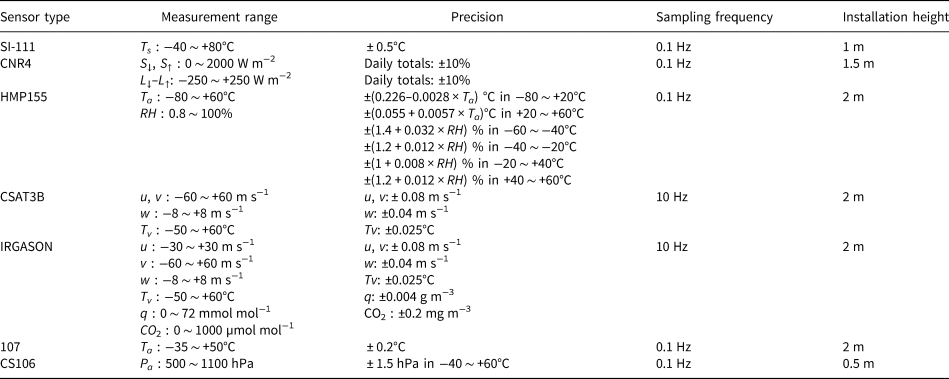
The observation site was located at a fixed landfast sea ice of East Antarctica, at 69°22′08.1″S, 76°21′42.1″E, and east of Amery ice shelf, northwest of Princess Elizabeth land, south of the Prydz bay (Fig. 1a). It is ~260 m from the nearest sea-ice edge (adjacent to land) and within 5 km from the nearest glacier on Princess Elizabeth land. During the observation period, the sea-ice thickness gradually increased from 0.5 m in April to 1.8 m in November with a mean value of 1.3 m. The mean snow thickness was 0.13 m, and the largest (smallest) monthly mean snow thickness of 0.35 (0.07) m occurred in July (November). A mast was installed on sea-ice surface, typically covered by snow, and the instruments on the mast included (Fig. 1c): an infrared radiometer SI-111, a net radiometer CNR4, a temperature and humidity sensor HMP155, a three-dimensional (3-D) sonic anemometer CSAT3B, and an in situ, open-path, mid-infrared gas (CO2/H2O) analyzer integrated with a 3-D sonic anemometer IRGASON. The IRGASON is controlled by the EC100 electronics, which uses inputs from a temperature thermistor probe 107 and a barometer CS106. The key technical specifications and installation height of these instruments can be found in Table 1. Additionally, the precipitation, which reported as snow water equivalent, used in this study is from the Russian Progress II station (located ~1 km from Zhongshan station). Consecutive observations were carried out from 8 April 2016 through 26 November 2016. Except for precipitation data, all the data were averaged every half hour, and data processing and quality control were carried out as follows:
(1) The spikes in the data series were removed by using a criterion of $X\,(t)\, \lt \,(\overline X + 4\sigma )$
 or $X(t) \gt (\overline X + 4\sigma )$, where X(t) denotes the measurements, $\overline X$ is the mean over the interval and σ is the Std dev..
(2) Surface turbulent fluxes were calculated by the eddy covariance method with 30 min averaging period. Turbulent data processing includes linear detrending, coordinate rotation, frequency correction, virtual temperature correction for sensible heat flux (SH hereafter) and WPL correction for latent heat flux (LE hereafter) (Lee, and others, Reference Lee, Massman and Law2004).
(3) Data quality control for eddy covariance measurements includes nonstationarity test, integrated turbulence characteristics test and horizontal wind angle test. After these three tests, the data are classified into nine grades. Foken and others (Reference Foken, Leuning, Oncley, Mauder, Aubinet, Aubinet, Vesala and Papale2012) suggested that classes 1–3 can be used for fundamental research, such as the development of parameterizations. Hence, only classes 1–3 of data were chosen in our research.


(a) The geographical location of observation site (the red dot), (b) the local topography and sketch of footprint with 50, 70, and 90% flux source areas (the blue circles), and (c) the meteorological tower at observation site.

The type of sensors and their key technical specifications
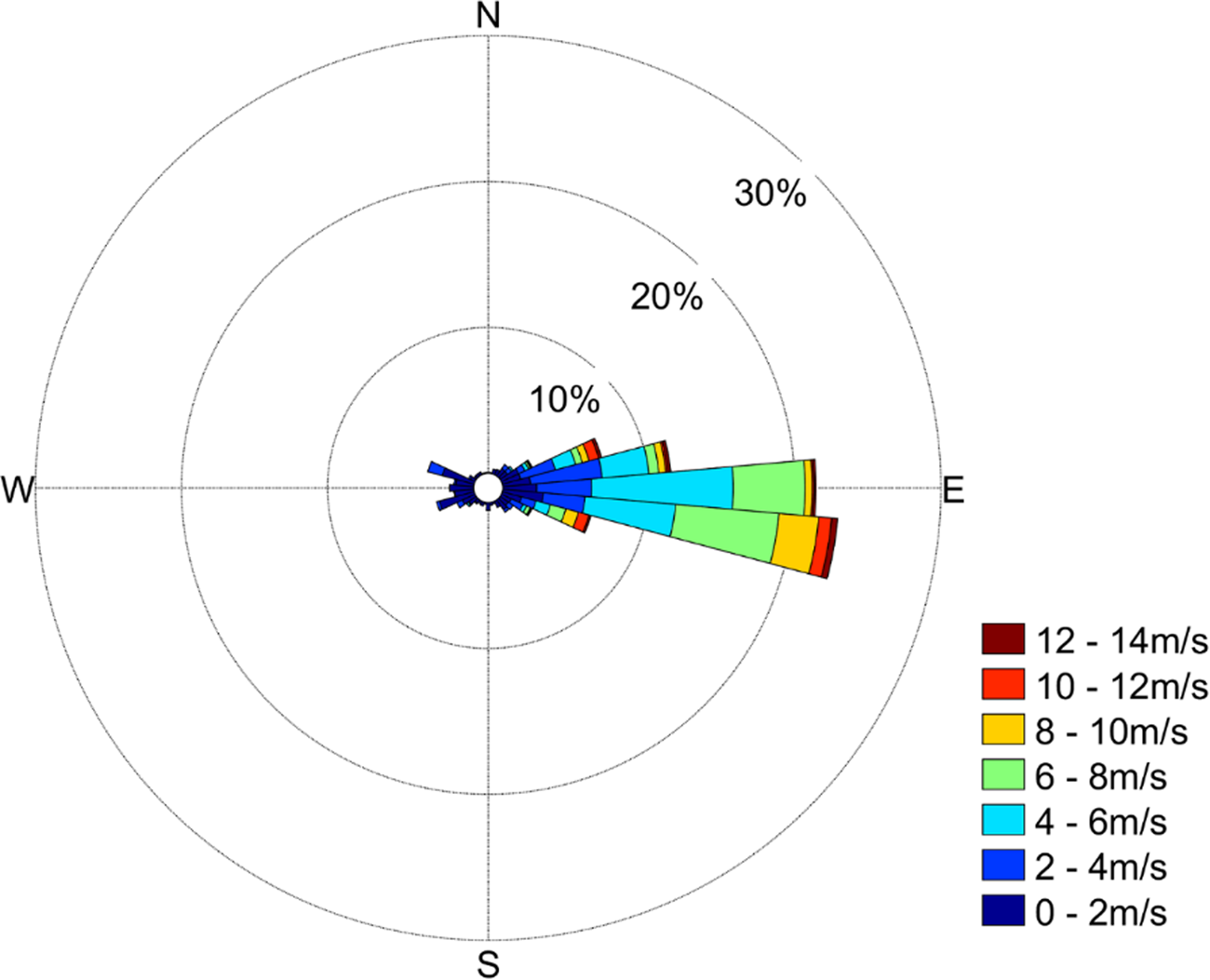
Additionally, the data in the sector of wind direction ranged from 65° to 115°, which account for 75% of total data (Fig. 2), were chosen to do footprint analysis by using the Kljun and others (Reference Kljun, Calanca, Rotach and Schmid2015) model. From Figure 1b, it can be seen that 90% of the measured flux was expected to come from within 250 m of the observation site. Within this fetch, it is entirely sea-ice surface.
Wind rose during the period from 8 April 2016 through 26 November 2016 at observation site.
2.2 Eddy covariance (EC) methods
EC method uses the turbulent fluctuations of meteorological elements measured by high frequency observation instruments to calculate surface turbulent fluxes,


where, τ (N m−2) is the turbulent momentum flux, w´ (m s−1), u´ (m s−1), θ´ (K), and q´ (kg kg−1) are the turbulent fluctuations of vertical velocity, horizontal velocity, potential temperature and specific humidity, respectively, ρ (kg m−3) is the air density, c p (J kg−1 K−1) is the constant-pressure specific heat capacity of air and λ (J kg−1) is the latent heat of vaporization. c p and λ can be calculated from Eqn (4) and (5),


where, c pb ( = 1004 J kg−1 K−1) and c pw ( = 1952 J kg−1 K−1) are the specific heat of dry and water vapor at constant pressure, respectively, ρ d (kg m−3) and ρ w (kg m−3) are the density of dry air and water vapor, respectively, T a (K) is the air temperature.
2.3 Bulk method
In the context of MOST, surface turbulent fluxes can be parameterized as,


where, u * (m s−1), T * (K), and q * (kg kg−1) are the frictional velocity, temperature scale, and specific humidity scale, respectively, u (m s−1) is the horizontal velocity, k ( = 0.4) is the von Kármán constant, z (m) is the observation height, z 0m (m), z 0h (m), and z 0q (m) are the aerodynamic roughness length, scalar roughness length for temperature and scalar roughness length for vapor water, respectively, L (m) is the Obukhov length, T s (K) is the surface temperature, q a (kg kg−1) and q s (kg kg−1) are the specific humidity at observation height and surface, respectively, R is the Prandtl number, g ( = 9.8 m s−2) is the gravitational constant, and ψ M, ψ H and ψ E are the integrated stability correction functions for wind, temperature and humidity, respectively. Because z 0q and ψ E are difficult to determine, the usual practice is to assume that z 0q = z 0h and ψ E = ψ H. Therefore, this paper will focus on the parameterization of τ and SH.
Stability correction functions and roughness lengths are two key issues in the Bulk method. Following stability correction functions for unstable stratification proposed by Cheng and Brutsaert (Reference Cheng and Brutsaert2005) and for stable stratification suggested by Paulson (Reference Paulson1970) are used in this study,


where, ζ ( = z/L) is the stability parameter, x = (1–16ζ)1/4 and y = (1–16ζ)1/2, a = 6.1, b = 2.5, c = 5.3, and d = 1.1.
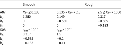
For roughness lengths, Andreas (Reference Andreas1987, hereafter as A87) proposed a theoretical model that predicts z 0h over ice surface from roughness Reynolds number (Re *),


where ν ( = 1.53 × 10⁻⁵ m2 s−1) is the air kinematic viscosity. The polynomial coefficients b 0, b 1 and b 2 are listed in Table 2. By using the data collected during the experiments in Greenland and Iceland, Smeets and Van den Broeke (Reference Smeets and Van den Broeke2008b, hereafter as S08) updated the polynomial coefficients for z 0h in Eqn (17). In addition, Zilitinkevich (Reference Zilitinkevich1995) proposed a simple Reynolds number-dependent formulation for all kinds of surface,

where C is an empirical constant and is equal to 0.8 in Zilitinkevich's study (hereafter as Z95). However, Chen and others (Reference Chen, Janjić and Mitchell1997, hereafter as C97) suggested C with the value of 0.1 can reduce forecast precipitation bias by conducting the National Center for Environmental Prediction (NCEP) mesoscale Eta forecast model. In addition, to predict the diurnal variation of z 0h, Yang and others (Reference Yang2007, hereafter as Y07) proposed a formulation to calculate z 0h over the bare-soil surface,

where β is a constant with the value of 7.2.
Values of the polynomial coefficients for z 0h in Eqn (13)
2.4 Surface energy balance
In this study, the surface energy balance (SEB) of sea ice is written as (Persson and others, Reference Persson, Fairall, Andreas, Guest and Perovic2002; Else and others, Reference Else2014),

where F net is the total energy flux into surface slab, S ↓, S ↑, L ↓ and L ↑ are downward shortwave radiation flux, upward shortwave radiation flux, downward longwave radiation flux and upward longwave radiation flux, respectively. G is the subsurface conductive heat flux. The unit of energy components in Eqn (21) is W m−2. In this SEB system, all terms on the right-hand side of Eqn (21) are defined positive when directed towards the surface. F net may be positive or negative. The positive F net indicates the snow or ice gains energy, which can be used to increase the temperature of surface slab, or melt when surface temperature is over melting point. The negative F net means energy loss, and ice growth or cooling surface slab. The conductive heat flux in Eqn 21 can be estimated as,

or

where, k s ( = 0.3 W m−1 °C−1) and k i ( = 2 W m−1 °C−1) are the thermal conductivity of snow and ice, respectively. T ice is the ice surface temperature and T w ( = −1.8°C) is the water temperature at the bottom of the ice. d s and d i are snow and ice thickness, respectively. It is noted that the value of k s is related to the physical properties of snowpack, for example snow density and humidity. Unfortunately, due to the lack of records of snow physical properties, we have to use the value of 0.3 W m−1 °C−1 for k s, which is typically used in large-scale sea-ice models (Toyota and others, Reference Toyota, Massom, Tateyama, Tamura and Fraser2011).
3. Results and discussion
3.1 Conventional meteorological conditions
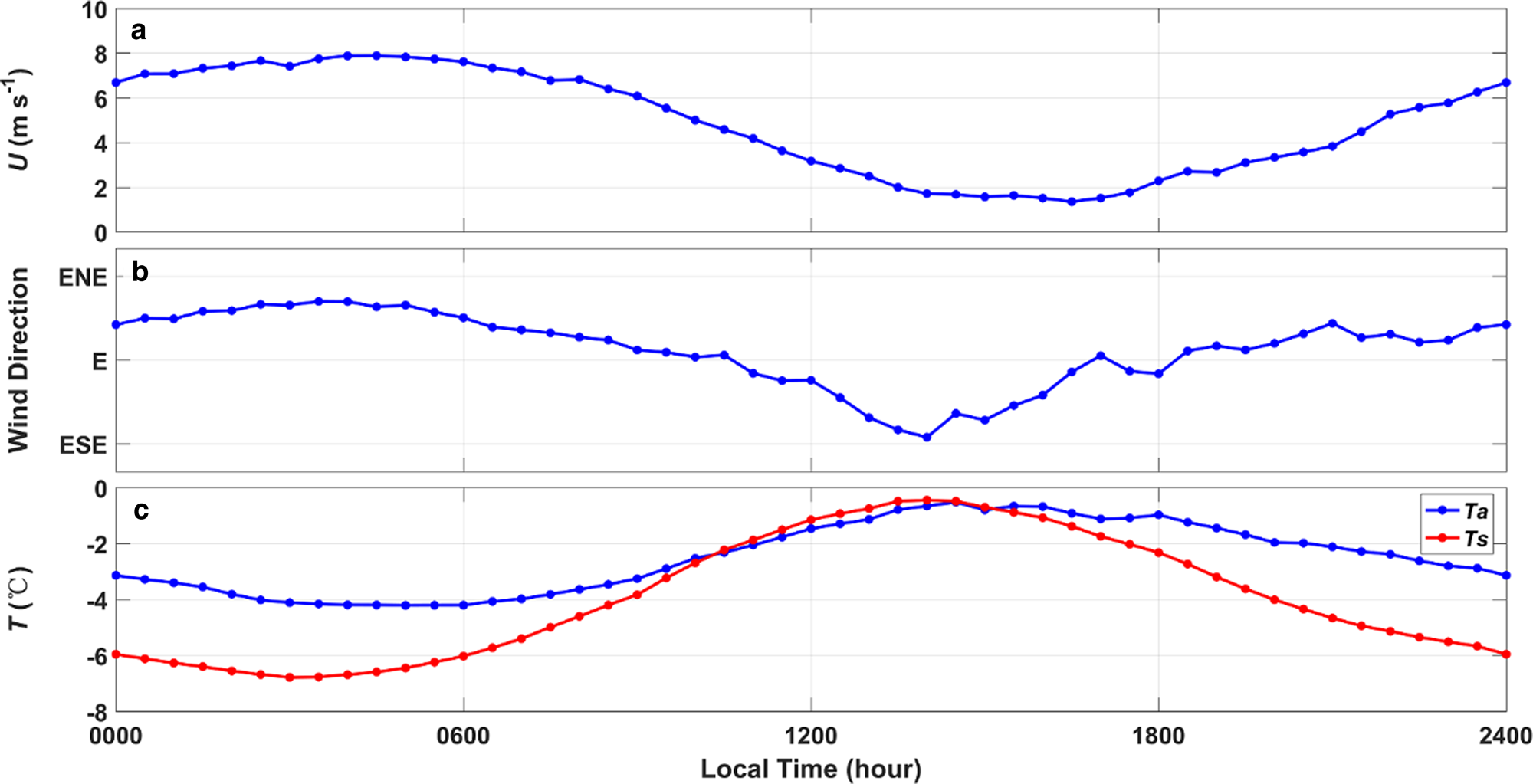
The easterlies prevailed during the whole observation period, as shown in Figure 2. The mean wind speed at 2 m height during the whole observation period was 4.2 m s−1, and the 4-hour-averaged maximum value could reach 13.9 m s−1. The largest (lowest) monthly mean wind speed of 6.0 (3.0) m s−1 occurred in August (July) (Fig. 3a). Especially, the wind speed in November showed a significant daily variation, which was related to the land-sea breeze. Figure 4a and 4b present the monthly mean diurnal variation of wind speed and wind direction in November, respectively. It can be seen that wind speed was higher in early morning and the monthly mean daily maximum wind speed reached 7.9 m s−1, while the monthly mean daily minimum wind speed of 1.4 m s−1 appeared in the afternoon. The wind direction also showed a diurnal variation from east-south-easterlies in the morning to east-north-easterlies in the afternoon.
Conventional meteorological data collected during the period from 8 April 2016 through 26 November 2016 at the observation site. (a), (b), (c), (d), (e) and (f) are the time series of 4-hourly average wind speed at 2 m height, air temperature (blue line) at 2 m height and surface temperature (red line), relative humidity at 2 m height, ambient air pressure at 0.5 m height, daily precipitation and daily sunshine time, respectively.

The mean diurnal variation of (a) wind speed, (b) wind direction and (c) temperature (blue line for air temperature and red line for surface temperature) in November 2016.

For temperature (Fig. 3b), the mean (4-hour-averaged maximum/minimum) air temperature at 2 m height during the whole observation period reached −15 (3/−40)°C. In contrast, the mean (4-hour-averaged maximum/minimum) surface temperature was a bit lower, being −17 (2/−48)°C. In November, the air temperature and surface temperature had clear diurnal variation, with monthly mean diurnal range of 3.7 and 6.3°C, respectively (Fig. 4c). The monthly mean daily maximum value of air temperature was close to that of surface temperature, but the monthly mean daily minimum value of air temperature and surface temperature was −4 and −7°C in November, respectively.
For relative humidity (Fig. 3c), the mean relative humidity at 2 m height during the whole observation period was 56%, and July (November) was the wettest (driest) month. For ambient air pressure (Fig. 3d), the mean ambient air pressure at 0.5 m height during the whole observation period was 978 hPa, and the lowest (highest) monthly mean ambient air pressure of 972 (986) hPa appeared in September (November). The total precipitation during the whole observation period was 156.9 mm, and concentrated in June (25.0 mm), July (44.1 mm) and October (24.2 mm). Figure 3f describes the variation of daily sunshine time and the sawteeth were caused by the sporadic clouds. It can be found that during the period from 7 May through 22 July was Polar night, and the monthly mean daily sunshine time reached 19 hours in November.
3.2 Radiation fluxes
Figure 5 presents the monthly mean diurnal variation of S ↓, S ↑, L ↓, L ↑, R n and albedo during the observation period. It can be seen from Figure 5a that there were significant differences in the monthly mean diurnal variation of S ↓ in different months. All days in June were Polar night, while the monthly mean daily maximum S ↓ reached 659 W m−2 in November. The monthly mean diurnal variation of S ↑ in different months also showed great distinctions, and the monthly mean daily maximum S ↑ reached −449 W m−2 in November (Fig. 5b). For L ↓ and L ↑ (Fig. 5c and 5d), the largest (smallest) monthly mean absolute value of L ↓ and L ↑ were 227 and 296 (176 and 222) W m−2, respectively, and both occurred in November (September). For R n (Fig. 5e), there was a sharp diurnal variation in September, October and November, and the monthly mean daily maximum R n in September, October and November were −10, 42 and 136 W m−2, respectively. The positive monthly mean R n only occurred in November, which was 21 W m−2. The smallest monthly mean R n, −58 W m−2, appeared in August. From Figure 5f, the highest monthly mean albedo, being 0.93, occurred in July. The albedo gradually decreased from July to October, reflecting the freezing process of accumulated snow (Yang and others, Reference Yang2016). While melting process changed the properties of ice surface, making the monthly mean albedo in November much smaller (0.69) than that in other months (>0.8).
The monthly mean diurnal variation of surface radiation fluxes and albedo during the observation period. (a), (b), (c), (d), (e) and (f) are the S ↓, S ↑, L ↓, L ↑, R n and albedo, respectively.

3.3 Turbulent fluxes and surface energy budget
The mean τ during the whole observation period was 0.15 N m−2, and the largest (smallest) monthly mean τ of 0.24 (0.1) N m−2 occurred in August (July). τ showed a significant monthly mean diurnal variation only in November (the pink line in Fig 6a), and the variation pattern was similar to that of the wind speed (Fig. 4a). The monthly mean daily maximum (minimum) τ in this month was 0.31 (0.03) N m−2. In November, because the surface snow around the observation site began to melt and the sea-ice area decreased, the thermal contrast between open ocean and land was intensified. Thus, a sea-land breeze might have modulated the near-surface wind and τ near the site.
The monthly mean diurnal variation of (a) τ (Tau), (b) SH and (c) LE during the observation period.
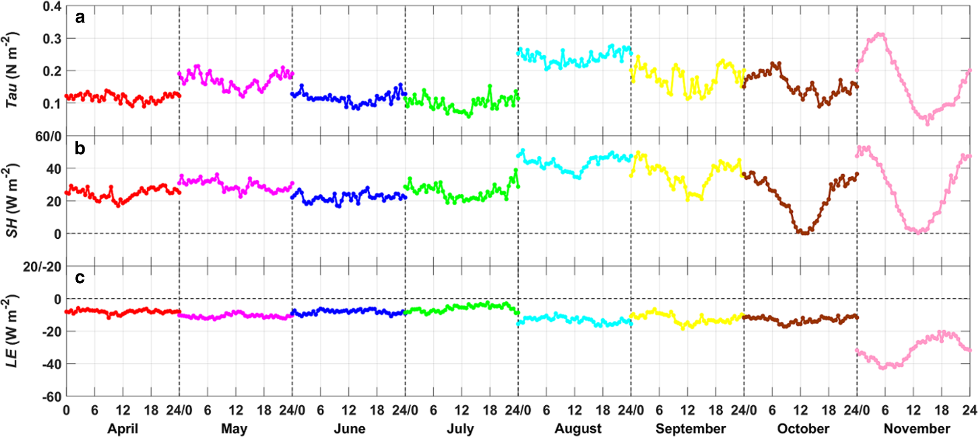
From Figure 6b, it can be found that the monthly mean SH was positive in each month during the observation period, which meant that the sea-ice surface generally absorbs sensible heat from atmosphere. The largest (smallest) monthly mean SH of 43 (21) W m−2 occurred in August (October). The mean value of SH in winter (June, July and August.) was 31 W m−2 that was significantly greater than that observed at the interior plateau (~12 W m−2) and was similar to that observed at katabatic wind zone (~32 W m−2) in Dronning Maud Land, East Antarctica (Van den Broeke and others, Reference Van den Broeke, van As, Reijmer and van de Wal2005). Our observation site is also located in katabatic wind zone, where strong winds frequently germinate. Van den Broeke and others (Reference Van den Broeke, van As, Reijmer and van de Wal2005) indicated that the katabatic winds vertically mix the air, which results in 5–10°C higher near-surface temperature than nonkatabatic wind region in Antarctica. Additionally, the warm signatures can also be found in katabatic wind region on satellite infrared imagery (King and others, Reference King, Varley and Lachlan-Cope1998). So, strong wind conditions are conductive to the enhancement of downward SH in Antarctica. There was a clear monthly mean diurnal variation in SH with a diurnal range of 29, 37 and 53 W m−2 in September, October and November, respectively (Fig. 6b). Contrary to SH, the monthly LE were negative in each month during the observation period (Fig. 6c), which meant that the sea-ice surface released mass to atmosphere through sublimation. The most significant sublimation appeared in November, with monthly mean LE of −32 W m−2. The monthly mean diurnal variation of LE in November was obvious and was closely related to wind speed.
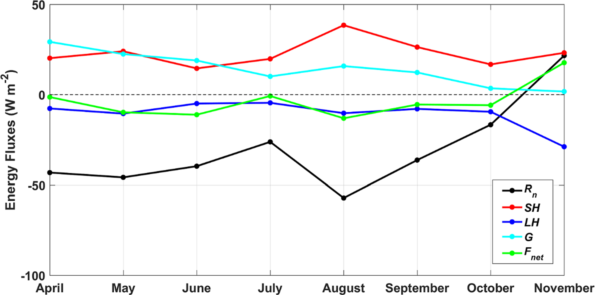
Figure 7 describes the monthly variation of the surface energy budget. From April to October, ice surface lost energy through R n and LE while obtained energy through SH and G, and SH was the main heat source of surface from July to October. On the other hand, the small negative F net appeared during the sea-ice growth period, and the mean value of F net from April to October was −7 W m−2. However, in November, the distinctly negative LE was the only heat sink of surface and F net turned to positive. The surplus energy was used for surface warming or melting as the surface temperature was first observed to reach 0°C on 1 November.
The monthly variation of R n, SH, LE, G and F net during the observation period.
To better understand the differences in snow or sea-ice processes, related to surface heat fluxes, between the Antarctica and the Arctic, two Arctic field experiments, included the Surface Heat Budget of the Arctic Ocean (SHEBA) and N-ICE2015 (a campaign focused on the surface energy budget over young, thin Arctic sea ice), were compared with our observation results. The statistics of SHEBA and N-ICE2015 were concluded from Persson and others (Reference Persson, Fairall, Andreas, Guest and Perovic2002) and Walden and others (Reference Walden, Hudson, Cohen, Murphy and Granskog2017). The monthly mean values of net shortwave radiation (NSR hereafter, NSR = S ↓–S ↑), net longwave radiation (NLR hereafter, NLR = L ↓–L ↑), R n, SH and LE from May to November (from November to May in SHEBA) were shown in Table 3. From May to August, the monthly mean NSR from our observation and SHEBA both were close to zero, surface radiation budget was dominated by longwave radiation. While, the monthly mean NSR in our observation was larger than that in SHEBA from September to November, because the location of SHEBA observation site was at higher latitudes (76–77° N). The NLR in our observation and SHEBA both were negative, which meant that surface lost energy through longwave radiation. In fact, the values of L ↓ and L ↑ both were larger in our observation, but the difference of L ↑ between our observation and SHEBA was greater than that of L ↓ in most months, which further lead to the larger negative NLR in our observation. However, the energy loss by NLR in July was the smallest in our observation and was equal to that in SHEBA, due to the frequent heavy precipitation events, which enhanced L ↓. R n was controlled by NSR and NLR, and showed the same direction but larger magnitude in our observation compared to that in SHEBA. Compared with the results of SHEBA, although the increase of L ↑ in our observation was greater than the increase of L ↓, the increase of air temperature was still greater than that of surface temperature because the effective longwave emissivity of the Polar atmosphere was much smaller than the emissivity of sea-ice surface. Therefore, the inversion temperature gradient in our observation was stronger, the stratification was more stable and the downward sensible heat flux was larger. In contrast to our results, the contribution of LE in surface heat budget in SHEBA were negligible, because the air was drier and the higher wind speed was conducive to evaporation in our observation.
The monthly mean values of net shortwave radiation (NSR), net longwave radiation (NLR), R n, SH, and LE from November to May for our observation results and the values in brackets were results from SHEBA
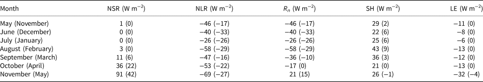
In a winter case study of N-ICE2015 campaign, the values of R n and SH were comparable to our results under clear skies and showed a larger magnitude than SHEBA. Graham and others (Reference Graham2017) attributed the differences between two Arctic experiments to the geographical location. The N-ICE2015 site was located close to the ice edge, where it allowed stronger winds and more advection of heat, but the SHEBA camp was located far from the ice edge. However, R n was near to 0 W m−2 and SH could reach −50 W m−2 during N-ICE2015 when the storm events occurred, due to the cloud over and cold air advection.
3.4 Roughness lengths
3.4.1 Aerodynamic roughness length z0m
The aerodynamic roughness length z 0m is an essential parameter in the calculation of turbulent fluxes by Bulk method. Under near-neutral condition (−0.01 ≤ ζ ≤ 0.01), Eqn (9) is written as,

then z 0m can be calculated with measured u * by EC method and wind speed u. It is found that large values of z 0m were concentrated in the direction of ESE to ES, while small values in NE to E (Fig. 8). However, there was no significant correlation between z 0m and wind speed. Such a distribution of z 0m might be caused by the orientation of surface undulating (e.g. Vignon and others, Reference Vignon2017). Our results indicate that the all-averaged value of z 0m was 1.9 × 10⁻³ m, with a range of uncertainty from 2.2 × 10⁻⁴ m to 5.4 × 10⁻³ m. This coincides reasonably well with the typical range of order of magnitude of z 0m, 1 × 10⁻⁴ m to 1 × 10⁻² m (Guest and Davidson, Reference Guest and Davidson1991), for the Antarctic sea-ice/snow surface. However, Andreas (Reference Andreas2011) pointed out that z 0m might be a site-dependent parameter, which depending on the surface elevation along upwind lines.
Distribution of z 0m under various wind speed and wind direction (the results were shown only when the number of sample in each bin is >5).
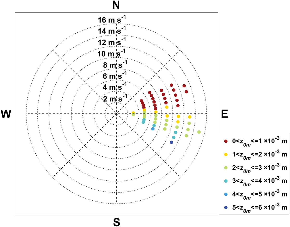
By analyzing the roughness of the snow-covered surface in the ablation zone of a Greenland ice sheet in the Arctic, Smeets and Van den Broeke (Reference Smeets and Van den Broeke2008a) concluded that melting snow could increase z 0m. Here, we calculated the mean value of z 0m by using the data before 1 November and after 1 November (when the surface temperature started to rise above 0°C), and the corresponding values were 1.8 × 10⁻³ m and 2.2 × 10⁻³ m, respectively. Hence, our results also showed that the aerodynamic roughness slightly increased due to snow melting. Unfortunately, the absence of summer observation prevented us from drawing a clear seasonal variation of z 0m. In fact, from the results of Wamser and Martinson (Reference Wamser and Martinson1993) and Weiss and others (Reference Weiss, King, Lachlan-Cope and Ladkin2011), it can be found that the value of z 0m for multiyear pack ice in Weddell Sea in summer (4.1 × 10⁻³ m) was of order of magnitude larger than in winter (4.7 × 10⁻⁴ m).
3.4.2 Scalar roughness length for temperature z 0h
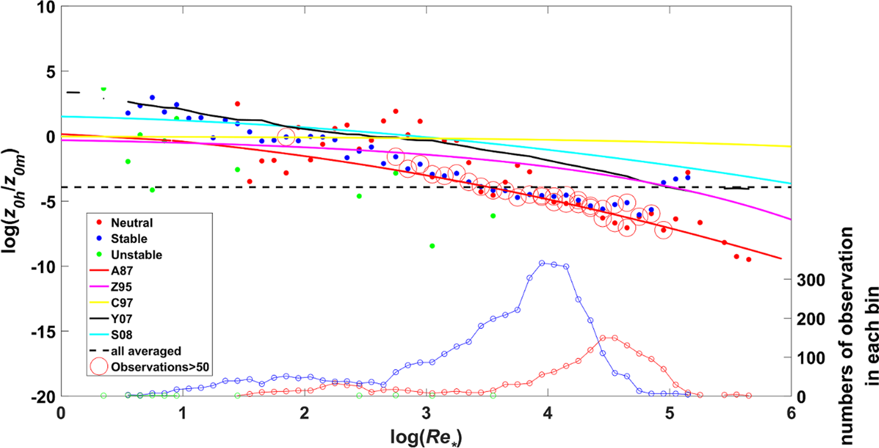
Based on the MOST, z 0h can be calculated by Eqn (10) and (12) with measured u *, T * and established stability correction functions. Figure 9 compares several popular parameterization schemes of log(z 0h/z 0m). It can be found that data were mainly concentrated on the range of log(Re *) from 2.5 to 5, corresponding to the rough surface. For the region of 2.5 < log(Re *) < 5, it is clear that A87 scheme made a good performance in the calculation of log(z 0h/z 0m), while other schemes all overestimated significantly. However, when log(Re *) ≤ 2.5, the bias and normalized standard error (NSE) of SH parameterized by Bulk method with C97 scheme were smallest (Table 4). The overall averaged log(z 0h/z 0m) = −3.93, which makes z 0h = 3.7 × 10⁻⁵ m. This value is two orders of magnitude lower than the value of 8 × 10⁻³ m obtained by Cassano and others (Reference Cassano, Parish and King2001) at Halley Research Station, but on the same order of magnitude as the value of 2.9 × 10⁻⁵ m at the west western part of Queen Maud Land, Antarctica, suggested by Bintanja and Van den Broeke (Reference Bintanja and Van den Broeke1995) or the value of 2.0 × 10⁻⁵ m found at Dome C, Antarctica, by Vignon and others (Reference Vignon2017).
The calculated log(z 0h/z 0m) versus log(Re *). The dots are the bin averaged log(z 0h/z 0m) with 0.1 interval of log(Re *) and red, blue and green colors represent for neutral, stable and unstable condition, respectively. Red circles indicate that the observation sample number in the bin is larger than 50. The red solid line, mauve solid line, yellow solid line, black solid line, cyan solid line and black dashed line are log(z 0h/z 0m) from A87, Z95, C97, Y07, S08 and whole averaged of original data, respectively. The sample numbers of neutral (red dot-dashed line), stable (blue dot-dashed line), and unstable (green dot-dashed line) condition in each bin are shown in the bottom part.
The regression slope, bias, and NSE of SH parameterized by Bulk method with various z 0h schemes in the different region of log(Re *)

Boldface numbers are the best among these schemes. Here, bias $= \mathop \sum \limits_{i = 1}^n \vert {SH_{{\rm EC}}-SH_{{\rm Bulk}}} \vert /n$ and NSE = $\sqrt {\mathop \sum \limits_{i = 1}^n {\vert {SH_{{\rm EC}}-SH_{{\rm Bulk}}} \vert }^2/\mathop \sum \limits_{i = 1}^n {\vert {SH_{{\rm EC}}} \vert }^2}$
 .
.
Large and others (Reference Large, Mc Williams and Doney1994) reported that z 0h existed considerable differences in orders of magnitude between unstable and stable stratification over the open ocean. Then, Andreas and others (Reference Andreas2010) first considered the stratification dependence of z 0h over sea ice. They found that the values of log(z 0h/z 0m) were larger under unstable stratification than under stable stratification by analyzing the data collected during SHEBA experiments, but they did not think the statistical results were enough conclusive. In this study, the mean value of log(z 0h/z 0m) under stable (ζ > 0.01), near-neutral (−0.01 ≤ ζ ≤ 0.01) and unstable (ζ < −0.01) stratification were −3.48, −5.01 and −1.20, respectively. However, because the amount of data under unstable stratification is too small to be convincing, the mean value of log(z 0h/z 0m) under unstable stratification is not discussed. Our results show that log(z 0h/z 0m) was larger under stable stratification than under near-neutral stratification and the significant difference has been proved through the Student's t test with 95% statistical confidence. A possible explanation is that, under near-neutral stratification, the stronger wind speed leads to the larger Re * and the increase of Re * will decrease log(z 0h/z 0m) according to Andreas (Reference Andreas1987). From Figure 9, we can also find that the data under near-neutral stratification were concentrated on the large Re * region.
4. Conclusions
By using the data observed over sea-ice surface near Zhongshan station during the period from 8 April 2016 through 26 November 2016, this study focuses on the status of surface energy budget and the crucial parameters, z 0m and z 0h, in the parameterization of turbulent fluxes, and we conclude the following:
During the whole observation period, the mean (4-hour-averaged maximum/minimum) wind speed and air temperature at 2 m height, and surface temperature were 4.2 (13.9/0) m s−1, −15 (3/−40)°C and −17 (2/−48)°C, respectively. In November, caused by the influence of local sea breeze, wind speed (wind direction) showed a significant daily variation. July (November) was the wettest (driest) month. The accumulated precipitation during the observation was 156.9 mm and concentrated in July. The monthly mean albedo decreased from 0.93 in July to 0.69 in November, which related to the snow melting process.
From April to October, most of the lost surface energy through LE and R n was balanced by SH and G, and F net was slightly negative. However, LE was the only heat sink of surface and F net turned to positive in November. The direction of energy fluxes in our study was generally consistent with previous studies both in the Antarctica and Arctic, but showed differences in magnitude. Our results support that the strong winds in the katabatic wind zone enhance the downward SH in Antarctica. Additionally, two Arctic experiments were compared with our observation. The results from SHEBA data showed smaller positive SH (negative LE), due to the colder air (wetter air and lower wind speed). While, the values of R n and SH in N-ICE2015 campaign were comparable to our results under clear skies, but SH turned to negative caused by the effects of cloud over and cold air advection during the storm events.
In this study, the mean value of z 0m was 1.9 × 10⁻³ m. It is found that z 0m did not vary with wind speed but changed with wind direction and snow melting might increase z 0m. Meanwhile, the all-averaged value of z 0h, being 3.7 × 10⁻⁵ m, was suggested in our study. Our results showed that the parametrization scheme of z 0h proposed by Andreas (Reference Andreas1987) made a better performance in the region of log(Re *) > 2.5 and Chen and others (Reference Chen, Janjić and Mitchell1997)'s scheme was more reasonable when log(Re *) ≤ 2.5. Additionally, the larger value of log(z 0h/z 0m) was found under stable stratification than under near-neutral stratification, due to the stronger winds under near-neutral stratification.
Although we have presented some observation results and analysis for surface energy budget and parameterization of near-surface turbulent fluxes over the Antarctic sea ice, the work of evaluating the numerical model [e.g. HIGHTSI model (a high-resolution thermodynamic snow and ice model)] has not been done at present, and this will be carried out in the future.
Acknowledgements
This work was jointly supported by the National Key Projects of Ministry of Science and Technology of China (2016YFA0602100), the Foundation of Key Laboratory of Land Surface Process and Climate Change in Cold and Arid Regions (LPCC2018001, LPCC2018005), the National Natural Science Foundation of China (41875013, 41941009, 41675015), the Fundamental Research Funds for the Central Universities (No. 19lgzd07), the Key Research Program of Frontier Sciences of CAS (QYZDY-SSW-DQC021), the Opening fund of State Key Laboratory of Cryospheric Science (SKLCS-OP-2019-09), and the Postgraduate Research & Practice Innovation Program of Jiangsu Province (KYCX18_1006). This is a contribution to the Year of Polar Prediction (YOPP), a flagship activity of the Polar Prediction Project (PPP), initiated by the World Weather Research Programme (WWRP) of the World Meteorological Organization (WMO). We thank the Chinese Arctic and Antarctic Administration and Polar Research Institute of China for the logistic support. We also thank the Russian meteorological station of Progress for providing precipitation data.
Author contributions
Changwei Liu performed most calculations and wrote the first version of the paper, Zhiqiu Gao made many constructive suggestions and helped improve the manuscript, Qinghua Yang provided most of the data and also participated in revising the manuscript, Bo Han, Hong Wang, Linlin Wang and Yubin Li helped revise the manuscript, Guanghua Hao, Jiechen Zhao and Lejiang Yu collected the data and conducted some calculations.


 Open access