


1 Introduction
In this article, we consider germs
 $\xi \in \text {Der}_{\mathbb R}(C^{\infty }(\mathbb R^{m},0))$
of smooth vector fields which admit an irreducible formal invariant curve, that is, a
$\xi \in \text {Der}_{\mathbb R}(C^{\infty }(\mathbb R^{m},0))$
of smooth vector fields which admit an irreducible formal invariant curve, that is, a
 $\Gamma \in \mathbb (\mathbb R[[t]])^{m}$
such that
$\Gamma \in \mathbb (\mathbb R[[t]])^{m}$
such that
 $(\hat \xi \circ \Gamma ) \wedge \Gamma '=0$
, where
$(\hat \xi \circ \Gamma ) \wedge \Gamma '=0$
, where
 $\hat \xi \in \text {Der}_{\mathbb R}(\mathbb R[[x_1,\ldots ,x_{m}]])$
is the Taylor expansion of
$\hat \xi \in \text {Der}_{\mathbb R}(\mathbb R[[x_1,\ldots ,x_{m}]])$
is the Taylor expansion of
 $\xi $
. The ordinary correspondence between formal series and asymptotic development suggests that there should be a real curve
$\xi $
. The ordinary correspondence between formal series and asymptotic development suggests that there should be a real curve
 $\gamma \subset \mathbb R^{m}$
, invariant by
$\gamma \subset \mathbb R^{m}$
, invariant by
 $\xi $
and asymptotic to
$\xi $
and asymptotic to
 $\Gamma $
. The main result in this paper proves that this intuition is actually true, under the hypothesis (in general, necessary) that
$\Gamma $
. The main result in this paper proves that this intuition is actually true, under the hypothesis (in general, necessary) that
 $\Gamma $
is not included in the formal singular locus of
$\Gamma $
is not included in the formal singular locus of
 $\xi $
: that is,
$\xi $
: that is,
 $\hat \xi \circ \Gamma \neq 0$
.
$\hat \xi \circ \Gamma \neq 0$
.
Theorem 1.1. Let
 $\xi $
be the germ of a
$\xi $
be the germ of a
 $C^{\infty }$
vector field at
$C^{\infty }$
vector field at
 $a\in \mathbb {R}^{m}$
, and let
$a\in \mathbb {R}^{m}$
, and let
 $\Gamma $
be a formal curve at a, invariant by
$\Gamma $
be a formal curve at a, invariant by
 $\xi $
, that is not included in the formal singular locus of
$\xi $
, that is not included in the formal singular locus of
 $\xi $
. Then there exists a germ of trajectory
$\xi $
. Then there exists a germ of trajectory
 $\gamma $
of
$\gamma $
of
 $\xi $
that is asymptotic to
$\xi $
that is asymptotic to
 $\Gamma $
.
$\Gamma $
.
In [Reference Bonckaert5], Bonckaert solves the three-dimensional case and asks whether this very natural result can be generalized to higher dimension (see [Reference Bonckaert5, Remark 2.4, p. 118]). A broader question, already addressed in that paper in dimension three, is to describe a realization of the ‘attracting basin’ of
 $\Gamma $
. We prove that such a realization exists as a topological manifold. In fact, there is one such manifold associated to each of the two half-branches of
$\Gamma $
. We prove that such a realization exists as a topological manifold. In fact, there is one such manifold associated to each of the two half-branches of
 $\Gamma $
(the formal analog of the connected components of
$\Gamma $
(the formal analog of the connected components of
 $\Gamma \setminus \{0\}$
when
$\Gamma \setminus \{0\}$
when
 $\Gamma $
converges). We postpone the precise definitions and a more accurate statement to § 5.
$\Gamma $
converges). We postpone the precise definitions and a more accurate statement to § 5.
Theorem 1.2. Let
 $\xi $
be a
$\xi $
be a
 $C^{\infty }$
vector field at
$C^{\infty }$
vector field at
 $a\in \mathbb {R}^{m}$
, and let
$a\in \mathbb {R}^{m}$
, and let
 $\Gamma $
be a formal curve at a, invariant by
$\Gamma $
be a formal curve at a, invariant by
 $\xi $
, such that
$\xi $
, such that
 $\widehat {\xi }\circ \Gamma \ne 0$
. For each half-branch
$\widehat {\xi }\circ \Gamma \ne 0$
. For each half-branch
 $\Gamma ^+$
of
$\Gamma ^+$
of
 $\Gamma $
, there is a finite order horn neighborhood
$\Gamma $
, there is a finite order horn neighborhood
 $V^+$
of
$V^+$
of
 $\Gamma ^+$
and a connected topological submanifold
$\Gamma ^+$
and a connected topological submanifold
 $S^+\subset V^+$
of positive dimension with the following property. For any
$S^+\subset V^+$
of positive dimension with the following property. For any
 $b\in V^+$
, the trajectory of
$b\in V^+$
, the trajectory of
 $\xi $
issued from b is asymptotic to
$\xi $
issued from b is asymptotic to
 $\Gamma ^+$
if and only if
$\Gamma ^+$
if and only if
 $b\in S^+$
and escapes from
$b\in S^+$
and escapes from
 $V^+$
otherwise.
$V^+$
otherwise.
Over the field of complex numbers
 $\mathbb C$
, one usually considers holomorphic vector fields, and the theory of Borel–Laplace multi-summability answers the analog question. Indeed, a (complex) formal series
$\mathbb C$
, one usually considers holomorphic vector fields, and the theory of Borel–Laplace multi-summability answers the analog question. Indeed, a (complex) formal series
 $\Gamma $
that is invariant by a (complex) analytic vector field
$\Gamma $
that is invariant by a (complex) analytic vector field
 $\xi $
, and not contained in
$\xi $
, and not contained in
 $\xi ^{-1}(0)$
, can be proved to be of Gevrey type and multi-summable. By a summation process such as that proposed, among others, by Balser [Reference Balser2], Braaksma [Reference Braaksma7], Ramis [Reference Ramis23] or Malgrange [Reference Malgrange22], we get invariant complex curves
$\xi ^{-1}(0)$
, can be proved to be of Gevrey type and multi-summable. By a summation process such as that proposed, among others, by Balser [Reference Balser2], Braaksma [Reference Braaksma7], Ramis [Reference Ramis23] or Malgrange [Reference Malgrange22], we get invariant complex curves
 $\gamma $
, defined and asymptotic to
$\gamma $
, defined and asymptotic to
 $\Gamma $
on some sectors. However, even if
$\Gamma $
on some sectors. However, even if
 $\xi $
and
$\xi $
and
 $\Gamma $
are real, these complex curves might not provide a (real) asymptotic trajectory if the so-called anti-Stokes directions of
$\Gamma $
are real, these complex curves might not provide a (real) asymptotic trajectory if the so-called anti-Stokes directions of
 $\Gamma $
contain the real one. So, even for real analytic vector fields, the theory of multi-summability does not solve the problem we address here. It should be mentioned that Ecalle proposed in [Reference Ecalle12] a strategy for a real resummation (see also [Reference Ecalle and Menous13]). Our approach circumvents the theory of resurgent functions.
$\Gamma $
contain the real one. So, even for real analytic vector fields, the theory of multi-summability does not solve the problem we address here. It should be mentioned that Ecalle proposed in [Reference Ecalle12] a strategy for a real resummation (see also [Reference Ecalle and Menous13]). Our approach circumvents the theory of resurgent functions.
Still in the real analytic setting, our result has application to tame geometry of trajectories, in the vein of [Reference Le Gal17–Reference Le Gal, Sanz and Speissegger20, Reference Rolin, Sanz and Schäfke25]. In the last section, we prove the following theorem.
Theorem 1.3. Let
 $\xi $
be a germ of analytic vector field at
$\xi $
be a germ of analytic vector field at
 $a\in \mathbb {R}^{m}$
, and let
$a\in \mathbb {R}^{m}$
, and let
 $\Gamma $
be a formal curve at a, invariant by
$\Gamma $
be a formal curve at a, invariant by
 $\xi $
, that is not contained in the singular locus of
$\xi $
, that is not contained in the singular locus of
 $\xi $
. Then there exists a germ of trajectory
$\xi $
. Then there exists a germ of trajectory
 $\gamma $
of
$\gamma $
of
 $\xi $
asymptotic to
$\xi $
asymptotic to
 $\Gamma $
and subanalytically non-oscillating (that is, for any subanalytic set A, the germ of
$\Gamma $
and subanalytically non-oscillating (that is, for any subanalytic set A, the germ of
 $A\cap \gamma $
is either empty or equal to
$A\cap \gamma $
is either empty or equal to
 $\gamma $
).
$\gamma $
).
We now outline the main steps of the proofs of Theorem 1.1 and Theorem 1.2.
After a sequence of admissible transformations (blow-ups and ramifications), we reduce the vector field
 $\xi $
in a neighborhood of the formal curve
$\xi $
in a neighborhood of the formal curve
 $\Gamma $
, in what we call a Turrittin–Ramis–Sibuya form (TRS for short). This reduction was inspired by Turrittin’s process [Reference Turrittin26] (see also Wasow [Reference Wasow30] or [Reference Balser2]), and developed for linear meromorphic differential equations over
$\Gamma $
, in what we call a Turrittin–Ramis–Sibuya form (TRS for short). This reduction was inspired by Turrittin’s process [Reference Turrittin26] (see also Wasow [Reference Wasow30] or [Reference Balser2]), and developed for linear meromorphic differential equations over
 $\mathbb C$
. Ramis and Sibuya in [Reference Ramis and Sibuya24], as well as Braaksma in [Reference Braaksma7], used such normal forms for their analysis of multi-summability of formal solutions of (nonlinear) meromorphic ordinary differential equations (ODEs). López-Hernanz, Ribón, Sanz Sánchez and Vivas present in [Reference López-Hernánz, Ribón, Sánchez and Vivas21] a reduction of the same nature for germs of holomorphic diffeomorphisms. For our purpose, it is necessary to retain the real structure, so we build on Barkatou, Carnicero and Sanz Sánchez [Reference Barkatou, Carnicero and Sanz Sánchez3], which gives a real reduction for linear formal meromorphic differential systems. Our reduction to real (TRS)-form for a
$\mathbb C$
. Ramis and Sibuya in [Reference Ramis and Sibuya24], as well as Braaksma in [Reference Braaksma7], used such normal forms for their analysis of multi-summability of formal solutions of (nonlinear) meromorphic ordinary differential equations (ODEs). López-Hernanz, Ribón, Sanz Sánchez and Vivas present in [Reference López-Hernánz, Ribón, Sánchez and Vivas21] a reduction of the same nature for germs of holomorphic diffeomorphisms. For our purpose, it is necessary to retain the real structure, so we build on Barkatou, Carnicero and Sanz Sánchez [Reference Barkatou, Carnicero and Sanz Sánchez3], which gives a real reduction for linear formal meromorphic differential systems. Our reduction to real (TRS)-form for a
 $C^\infty $
vector field along a formal invariant curve is presented in § 2.
$C^\infty $
vector field along a formal invariant curve is presented in § 2.
Once the vector field is reduced, our general strategy to construct the curve
 $\gamma $
is to work inductively on the dimension of the ambient space, by restriction to a center manifold, until this dimension drops to one or
$\gamma $
is to work inductively on the dimension of the ambient space, by restriction to a center manifold, until this dimension drops to one or
 $\Gamma $
is tangent to a non-zero eigenvalue (see Lemma 3.4 in § 3). In ambient dimension
$\Gamma $
is tangent to a non-zero eigenvalue (see Lemma 3.4 in § 3). In ambient dimension
 $m=2$
, a vector field in (TRS)-form is either hyperbolic or has a center manifold of dimension one, so the result is a consequence of the classical theory of invariant manifolds (for example, in [Reference Hirsch, Pugh and Shub15]). In higher dimension, this approach leads to two main difficulties. First, no smooth center manifold exists in general (see [Reference van Strien28]), so we have to consider vector fields of finite differentiability class.
$m=2$
, a vector field in (TRS)-form is either hyperbolic or has a center manifold of dimension one, so the result is a consequence of the classical theory of invariant manifolds (for example, in [Reference Hirsch, Pugh and Shub15]). In higher dimension, this approach leads to two main difficulties. First, no smooth center manifold exists in general (see [Reference van Strien28]), so we have to consider vector fields of finite differentiability class.
A more serious obstruction appears when the center manifold is the full ambient space (all eigenvalues have zero real part) because, in this case, the induction is interrupted. Thus, we need new arguments to treat the so-called dominant rotation case, excluded in Lemma 3.4, that is, when
 $\xi $
has only eigenvalues with pure imaginary initial part. In dimension three, this situation corresponds to the rotation case of [Reference Bonckaert5, IV (2.2) p. 134], treated separately by Bonckaert and Dumortier in [Reference Bonckaert and Dumortier6]. The strategy proposed in that paper consists of building an invariant slow manifold—that is, tangent to the kernel of the linear part of
$\xi $
has only eigenvalues with pure imaginary initial part. In dimension three, this situation corresponds to the rotation case of [Reference Bonckaert5, IV (2.2) p. 134], treated separately by Bonckaert and Dumortier in [Reference Bonckaert and Dumortier6]. The strategy proposed in that paper consists of building an invariant slow manifold—that is, tangent to the kernel of the linear part of
 $\xi $
—in a similar way to how center manifolds are constructed in the general theory. In higher dimensions, different rotations with different orders might compete with many real slow directions of different orders, and calculation of the required estimates seems impracticable.
$\xi $
—in a similar way to how center manifolds are constructed in the general theory. In higher dimensions, different rotations with different orders might compete with many real slow directions of different orders, and calculation of the required estimates seems impracticable.
To deal with this, we introduce in § 4 special kinds of transformations that we call straighteners. These act as a direct sum of plane rotations over a fibration transverse to
 $\Gamma $
so as to annihilate the spiraling effect induced by the pure imaginary eigenvalues. These transformations are strongly irregular and do not admit even a continuous extension at the singular point. However, in a neighborhood of each half-branch of
$\Gamma $
so as to annihilate the spiraling effect induced by the pure imaginary eigenvalues. These transformations are strongly irregular and do not admit even a continuous extension at the singular point. However, in a neighborhood of each half-branch of
 $\Gamma $
,
$\Gamma $
,
 $\xi $
has a lift of any finite differentiability class by the convenient straightener, and this lift has no more dominant rotation, up to first reducing to a stronger (TRS)-form (the class depends on the strength). From here, the induction can be continued. In this way, we produce trajectories with high but finite contact order with
$\xi $
has a lift of any finite differentiability class by the convenient straightener, and this lift has no more dominant rotation, up to first reducing to a stronger (TRS)-form (the class depends on the strength). From here, the induction can be continued. In this way, we produce trajectories with high but finite contact order with
 $\Gamma $
.
$\Gamma $
.
Our final argument to get trajectories asymptotic to
 $\Gamma $
is based on the existence of the so-called accompanying curves in the center manifold, which permits us to show that all trajectories with a sufficiently high contact with
$\Gamma $
is based on the existence of the so-called accompanying curves in the center manifold, which permits us to show that all trajectories with a sufficiently high contact with
 $\Gamma $
have flat contact with each other (cf. point (ii) in Lemma 3.4 and Lemma 4.3). In § 3, we recall the basics about accompanying curves, deduced from a fine treatment of the principle of reduction to a center manifold by Carr [Reference Carr10]. This approach has already been used by Cano, Moussu and Sanz in [Reference Cano, Moussu and Sanz9] for three-dimensional analytic vector fields. In this paper, we adapt Carr’s construction in order to obtain, in addition, the manifold
$\Gamma $
have flat contact with each other (cf. point (ii) in Lemma 3.4 and Lemma 4.3). In § 3, we recall the basics about accompanying curves, deduced from a fine treatment of the principle of reduction to a center manifold by Carr [Reference Carr10]. This approach has already been used by Cano, Moussu and Sanz in [Reference Cano, Moussu and Sanz9] for three-dimensional analytic vector fields. In this paper, we adapt Carr’s construction in order to obtain, in addition, the manifold
 $S^+$
of Theorem 1.2. A precise statement and the details are discussed in § 5.
$S^+$
of Theorem 1.2. A precise statement and the details are discussed in § 5.
It would be interesting to extend our result to more general types of series, for example, to allow real exponents or for more general formal transseries. The later needs an extended notion of being asymptotic, a question that has been considered by vdHoeven in [Reference van der Hoeven27] and by Aschenbrenner, vdDries and vdHoeven in [Reference Aschenbrenner, van den Dries and van der Hoeven1] in the context of polynomial ODEs over Hardy fields.
1.1 Notation
Consider a
 $C^{\infty }$
manifold M of dimension m and
$C^{\infty }$
manifold M of dimension m and
 $a\in M$
. We often put
$a\in M$
. We often put
 $m=1+n$
and have a local system of coordinates
$m=1+n$
and have a local system of coordinates
 $(x,y_1,\ldots ,y_n):M\to \mathbb R^{1+n}$
, centered at a, with a distinguished first coordinate. For short, we use a bold letter to refer to the tuple whose components are written with the same letter and subscripts:
$(x,y_1,\ldots ,y_n):M\to \mathbb R^{1+n}$
, centered at a, with a distinguished first coordinate. For short, we use a bold letter to refer to the tuple whose components are written with the same letter and subscripts:
 ${\mathbf {y}}=(y_1,\ldots ,y_n)$
. We also use subscripts to indicate coordinates or tuples of coordinates of a given object, for example, a parameterized curve
${\mathbf {y}}=(y_1,\ldots ,y_n)$
. We also use subscripts to indicate coordinates or tuples of coordinates of a given object, for example, a parameterized curve
 $\gamma :\mathbb R \to M$
might be written with no other precision as
$\gamma :\mathbb R \to M$
might be written with no other precision as
 $(\gamma _x,\gamma _{{\mathbf {y}}})$
.
$(\gamma _x,\gamma _{{\mathbf {y}}})$
.
The differential of a map f at a point a is written
 $df(a)\in (T_aM)^*$
, where
$df(a)\in (T_aM)^*$
, where
 $(T_aM)^*$
is the cotangent space of M at a; a might be omitted depending on the context. We use symbolic powers for diagonal k-tuples, that is,
$(T_aM)^*$
is the cotangent space of M at a; a might be omitted depending on the context. We use symbolic powers for diagonal k-tuples, that is,
 $d^kf(a)(v^{(k)})$
is the value of the kth differential of f over the k-tuple of direction
$d^kf(a)(v^{(k)})$
is the value of the kth differential of f over the k-tuple of direction
 $(v,v,\ldots ,v)\in (T_aM)^k$
. Given coordinates
$(v,v,\ldots ,v)\in (T_aM)^k$
. Given coordinates
 $(x,{\mathbf {y}})$
, the dual basis of
$(x,{\mathbf {y}})$
, the dual basis of
 $(dx,d{\mathbf {y}})$
is denoted by
$(dx,d{\mathbf {y}})$
is denoted by
 $(\partial _x,\partial _{{\mathbf {y}}})=(\partial _x,\partial _{y_1},\ldots ,\partial _{y_n})$
. We write the action of derivations as a product or with parenthesis, so
$(\partial _x,\partial _{{\mathbf {y}}})=(\partial _x,\partial _{y_1},\ldots ,\partial _{y_n})$
. We write the action of derivations as a product or with parenthesis, so
 $\partial _{{\mathbf {y}}}(f)=df(\partial _{{\mathbf {y}}})=(\partial _{y_1}f,\ldots ,\partial _{y_n}f)$
, which is not to be confused with the composition. For example,
$\partial _{{\mathbf {y}}}(f)=df(\partial _{{\mathbf {y}}})=(\partial _{y_1}f,\ldots ,\partial _{y_n}f)$
, which is not to be confused with the composition. For example,
 $\xi \circ \gamma $
is the value of
$\xi \circ \gamma $
is the value of
 $\xi \in \text {Der}_{\mathbb R}(C^{\infty }(M))$
over the parameterized curve
$\xi \in \text {Der}_{\mathbb R}(C^{\infty }(M))$
over the parameterized curve
 $\gamma $
; for the later we might also use restriction notation, for example,
$\gamma $
; for the later we might also use restriction notation, for example,
 $\xi _{|a}$
is the value of
$\xi _{|a}$
is the value of
 $\xi $
at a. We use a generic
$\xi $
at a. We use a generic
 $\cdot $
symbol to indicate a dot product on diverse tuples (such as matrices and vectors). Together with the bold notation and automatic definitions by subscript, we get compact expressions such as
$\cdot $
symbol to indicate a dot product on diverse tuples (such as matrices and vectors). Together with the bold notation and automatic definitions by subscript, we get compact expressions such as
 $\xi = \xi _x \partial _{x}+\xi _{{\mathbf {y}}}\cdot \partial _{{\mathbf {y}}}$
, where
$\xi = \xi _x \partial _{x}+\xi _{{\mathbf {y}}}\cdot \partial _{{\mathbf {y}}}$
, where
 $\xi _x = \xi (x)$
and
$\xi _x = \xi (x)$
and
 $\xi _{{\mathbf {y}}}=\xi ({\mathbf {y}})$
are implicitly defined once
$\xi _{{\mathbf {y}}}=\xi ({\mathbf {y}})$
are implicitly defined once
 $\xi \in \text {Der}_{\mathbb R}(C^{\infty }(M))$
and
$\xi \in \text {Der}_{\mathbb R}(C^{\infty }(M))$
and
 $(x,{\mathbf {y}})$
are given.
$(x,{\mathbf {y}})$
are given.
We use multi-indices for higher-order derivatives, that is, if
 $\alpha =(\alpha _0,\ldots ,\alpha _n)\in \mathbb N^{1+n}$
, then we set
$\alpha =(\alpha _0,\ldots ,\alpha _n)\in \mathbb N^{1+n}$
, then we set
 $|\alpha |=\sum _{j=0}^{n} \alpha _j$
and
$|\alpha |=\sum _{j=0}^{n} \alpha _j$
and
 $(x,{\mathbf {y}})^{\alpha }=x^{\alpha _0}y_1^{\alpha _1}\cdots y_n^{\alpha _n}$
and then
$(x,{\mathbf {y}})^{\alpha }=x^{\alpha _0}y_1^{\alpha _1}\cdots y_n^{\alpha _n}$
and then
 $$ \begin{align*} \partial^{|\alpha|}_{(x,{\mathbf{y}})^{\alpha}} = (\partial_x)^{\alpha_0}(\partial_{y_1})^{\alpha_1}\cdots(\partial_{y_n})^{\alpha_n}. \end{align*} $$
The jet
 $j_k f$
at
$j_k f$
at
 $(0,\boldsymbol {0})$
of order k of a function f is the polynomial
$(0,\boldsymbol {0})$
of order k of a function f is the polynomial
 $$ \begin{align*} j_kf(0,\boldsymbol{0})(x,{\mathbf{y}}) = \sum_{j\le k}\dfrac{1}{j!} d^{j}f(0,\boldsymbol{0})((x,{\mathbf{y}})^{(j)}) = \sum_{|\alpha|\le k} \dfrac{1}{|\alpha|!}(\partial^{|\alpha|}_{(x,{\mathbf{y}})^{\alpha}}{f})(0,\boldsymbol{0}) (x,{\mathbf{y}})^{\alpha}, \end{align*} $$
and the Taylor expansion of f is written as
 $\widehat {f}$
. We identify polynomials and polynomial functions, so
$\widehat {f}$
. We identify polynomials and polynomial functions, so
 $\mathbb R[x,{\mathbf {y}}]$
is seen as a subset of both formal series
$\mathbb R[x,{\mathbf {y}}]$
is seen as a subset of both formal series
 $\mathbb R[[x,{\mathbf {y}}]]$
and smooth functions
$\mathbb R[[x,{\mathbf {y}}]]$
and smooth functions
 $C^{\infty }(\mathbb R^{1+n})$
. We write
$C^{\infty }(\mathbb R^{1+n})$
. We write
 $\mathbb R_k[x]$
for the set of polynomials of (total) degree at most k.
$\mathbb R_k[x]$
for the set of polynomials of (total) degree at most k.
We use Landau notation o and O in the
 $C^{\infty }$
context, locally at a:
$C^{\infty }$
context, locally at a:
 $f=O(g)$
(respectively,
$f=O(g)$
(respectively,
 $f=o(g)$
) if there exists a bounded function h (respectively, h tends to
$f=o(g)$
) if there exists a bounded function h (respectively, h tends to
 $0$
) such that
$0$
) such that
 $f=gh$
in a neighborhood of a. Notice that when g is a power of a coordinate function, say
$f=gh$
in a neighborhood of a. Notice that when g is a power of a coordinate function, say
 $g=x^k$
,
$g=x^k$
,
 $f=O(x^k)$
(respectively,
$f=O(x^k)$
(respectively,
 $f=o(x^k)$
) implies that f is divisible by
$f=o(x^k)$
) implies that f is divisible by
 $x^k$
; that is,
$x^k$
; that is,
 $f=x^kh$
with a
$f=x^kh$
with a
 $C^{\infty }$
function h. We also use Landau notation to compare formal series with powers of coordinates, which of course implies divisibility in the ring
$C^{\infty }$
function h. We also use Landau notation to compare formal series with powers of coordinates, which of course implies divisibility in the ring
 $\mathbb R[[x,{\mathbf {y}}]]$
. Also, if
$\mathbb R[[x,{\mathbf {y}}]]$
. Also, if
 $f=f(x)$
is a
$f=f(x)$
is a
 $C^\infty $
germ of function at
$C^\infty $
germ of function at
 $x=0$
or a formal series in the variable x, we denote by
$x=0$
or a formal series in the variable x, we denote by
 $\text {ord}_x(f)$
the maximum
$\text {ord}_x(f)$
the maximum
 $k\in \mathbb {N}\cup \{\infty \}$
such that
$k\in \mathbb {N}\cup \{\infty \}$
such that
 $x^k$
divides f.
$x^k$
divides f.
Given a ring R,
 $\mathcal {M}_n(R)$
and
$\mathcal {M}_n(R)$
and
 $\text {GL}_n(R)$
refer, respectively, to
$\text {GL}_n(R)$
refer, respectively, to
 $n\times n$
matrices with coefficients in R and invertible such matrices. We write
$n\times n$
matrices with coefficients in R and invertible such matrices. We write
 $I_n$
for the identity matrix in
$I_n$
for the identity matrix in
 $\text {GL}_n(R)$
. We now introduce some useful notation concerning real and complex matrices. Recall that
$\text {GL}_n(R)$
. We now introduce some useful notation concerning real and complex matrices. Recall that
 $\Theta : \mathbb C\ni a+ib \mapsto a I_2+ b J_2\in \mathcal {M}_2(\mathbb R)$
is an isomorphism between
$\Theta : \mathbb C\ni a+ib \mapsto a I_2+ b J_2\in \mathcal {M}_2(\mathbb R)$
is an isomorphism between
 $\mathbb C$
and the subspace of
$\mathbb C$
and the subspace of
 $\mathcal {M}_2(\mathbb R)$
spanned by
$\mathcal {M}_2(\mathbb R)$
spanned by
 $I_2, J_2$
, with
$I_2, J_2$
, with
 $$ \begin{align*} I_2= \begin{pmatrix} 1 & 0 \\ 0 & 1 \end{pmatrix} \quad\text{and}\quad J_2 = \begin{pmatrix} 0 & -1 \\ 1 & 0 \end{pmatrix}. \end{align*} $$
We extend
 $\Theta $
first to formal series by setting, if
$\Theta $
first to formal series by setting, if
 $h(x)\in \mathbb C[[x]]$
,
$h(x)\in \mathbb C[[x]]$
,
 $\Theta (h(x))=\text {Re}(h(x))I_2+\text {Im}(h(x))J_2$
. Then we let
$\Theta (h(x))=\text {Re}(h(x))I_2+\text {Im}(h(x))J_2$
. Then we let
 $\Theta $
act on each coefficient of a given matrix
$\Theta $
act on each coefficient of a given matrix
 $M\in \mathcal {M}_m(\mathbb C[[x]])$
to define
$M\in \mathcal {M}_m(\mathbb C[[x]])$
to define
 $\Theta (M)$
, a matrix a priori in
$\Theta (M)$
, a matrix a priori in
 $\mathcal {M}_m(\mathcal {M}_2(\mathbb R[[x]]))$
space that we identify with
$\mathcal {M}_m(\mathcal {M}_2(\mathbb R[[x]]))$
space that we identify with
 $\mathcal {M}_{2m}(\mathbb R[[x]])$
. In this way, for each
$\mathcal {M}_{2m}(\mathbb R[[x]])$
. In this way, for each
 $m\ge 1$
,
$m\ge 1$
,
 $\Theta $
defines an injective morphism of
$\Theta $
defines an injective morphism of
 $\mathbb R$
-algebras between
$\mathbb R$
-algebras between
 $\mathcal {M}_m(\mathbb C[[x]])$
and
$\mathcal {M}_m(\mathbb C[[x]])$
and
 $\mathcal {M}_{2m}(\mathbb R[[x]])$
.
$\mathcal {M}_{2m}(\mathbb R[[x]])$
.
Since we work with block-shaped matrices, it is convenient to use the notation
 $M\oplus N$
for the matrix
$M\oplus N$
for the matrix
 $$ \begin{align*} M\oplus N=\begin{pmatrix} M & 0 \\ 0 & N \end{pmatrix} \in \mathcal M_{m+n}(R), \end{align*} $$
whenever
 $M\in \mathcal M_m(R)$
and
$M\in \mathcal M_m(R)$
and
 $N\in \mathcal M_n(R)$
. If D is diagonal by blocks, of the form
$N\in \mathcal M_n(R)$
. If D is diagonal by blocks, of the form
 ${D = \Theta (c_1 I_{n_{1}}\oplus \cdots \oplus c_{k} I_{n_{k}}) \oplus d_1 I_{m_1}\oplus \cdots \oplus d_{k'} I_{m_{k'}}}$
, we say that C has a block structure compatible with D (or that C is compatible with D, for short) whenever
${D = \Theta (c_1 I_{n_{1}}\oplus \cdots \oplus c_{k} I_{n_{k}}) \oplus d_1 I_{m_1}\oplus \cdots \oplus d_{k'} I_{m_{k'}}}$
, we say that C has a block structure compatible with D (or that C is compatible with D, for short) whenever
 $C = \Theta (C_1\oplus C_2\oplus \cdots \oplus C_k)\oplus E_1\oplus \cdots \oplus E_{k'}$
where, for all j,
$C = \Theta (C_1\oplus C_2\oplus \cdots \oplus C_k)\oplus E_1\oplus \cdots \oplus E_{k'}$
where, for all j,
 $C_j\in \mathcal M_{n_j}(R)$
and
$C_j\in \mathcal M_{n_j}(R)$
and
 $E_j\in \mathcal M_{m_j}(R)$
. If C is compatible with D, then
$E_j\in \mathcal M_{m_j}(R)$
. If C is compatible with D, then
 $[D,C]=0$
.
$[D,C]=0$
.
2 Reduction to (TRS) form
In this section, we give a procedure to transform a
 $C^{\infty }$
vector field along an invariant formal curve to another one with a useful expression in local coordinates. In the first subsection, we summarize the results of [Reference Barkatou, Carnicero and Sanz Sánchez3] on which we base our reduction. In a second subsection, we introduce the transformations that are admissible for a couple formed by a vector field and a non-singular invariant curve. Finally, we explain how to reduce a given vector field in a ‘neighborhood’ of an invariant formal curve (Theorem 2.6).
$C^{\infty }$
vector field along an invariant formal curve to another one with a useful expression in local coordinates. In the first subsection, we summarize the results of [Reference Barkatou, Carnicero and Sanz Sánchez3] on which we base our reduction. In a second subsection, we introduce the transformations that are admissible for a couple formed by a vector field and a non-singular invariant curve. Finally, we explain how to reduce a given vector field in a ‘neighborhood’ of an invariant formal curve (Theorem 2.6).
2.1 Real Turrittin’s theorem for linear systems of ODEs
The reduction we are looking for is based mainly on a result by Barkatou, Carnicero and Sanz [Reference Barkatou, Carnicero and Sanz Sánchez3], which we discuss briefly in this paragraph. It consists of a version of a classical Turrittin’s result on normal forms of formal meromorphic linear systems of ODEs (see [Reference Balser2, Reference Turrittin26, Reference Wasow30]) when the base field of coefficients is
 $\mathbb {R}$
.
$\mathbb {R}$
.
Consider a formal linear system of n ODEs of the form
 $$ \begin{align*} (S)\;\;\;\;\;x^{p+1}\boldsymbol{y}'=A(x)\cdot\boldsymbol{y}, \end{align*} $$
where
 $\boldsymbol {y} =(y_1,\ldots ,y_n)\in \mathbb R^{n}$
, the apostrophe denotes the derivative with respect to x, p is an integer and
$\boldsymbol {y} =(y_1,\ldots ,y_n)\in \mathbb R^{n}$
, the apostrophe denotes the derivative with respect to x, p is an integer and
 $A(x)\in \mathcal {M}_{n}(\mathbb {R}[[x]])$
, with
$A(x)\in \mathcal {M}_{n}(\mathbb {R}[[x]])$
, with
 $A(0)\neq 0$
. The system (S) is called singular if
$A(0)\neq 0$
. The system (S) is called singular if
 $p\ge 0$
and, in this case, following, for example, [Reference Balser2], the number p is called the Poincaré rank of the system (S). Otherwise, if
$p\ge 0$
and, in this case, following, for example, [Reference Balser2], the number p is called the Poincaré rank of the system (S). Otherwise, if
 $p<0$
, then we say that the system (S) is regular.
$p<0$
, then we say that the system (S) is regular.
The reduction is obtained by applying to the system certain transformations of the following kind.
-
(1) Gauge transformations. If
 $T=T(x)\in \text {GL}_n(\mathbb {R}[[x]][x^{-1}])$
, the change of variables
$\boldsymbol {y}=T(x)\cdot \boldsymbol {z}$
gives rise to a bijection
$\Psi _{T}$
between the whole family of systems, called a gauge transformation. Explicitly, it maps the system
$(S)\, x^{p+1}\boldsymbol {y}'=A(x)\cdot \boldsymbol {y}$
to the system
$(\widetilde {S})\, x^{\widetilde {p}+1}\boldsymbol {z}'=B(x)\cdot \boldsymbol {z}$
, where
$\widetilde {p}\in \mathbb {Z}$
and
$B(x)\in \mathcal {M}_n(\mathbb {R}[[x]])$
are chosen so that We consider the following two types of gauge transformations.
$$ \begin{align*} x^{-(\widetilde{p}+1)}B(x)=x^{-(p+1)}T(x)^{-1}A(x)T(x)-T(x)^{-1}T'(x)\quad \text{and}\quad B(0)\ne 0. \end{align*} $$
$T=T(x)\in \text {GL}_n(\mathbb {R}[[x]][x^{-1}])$
, the change of variables
$\boldsymbol {y}=T(x)\cdot \boldsymbol {z}$
gives rise to a bijection
$\Psi _{T}$
between the whole family of systems, called a gauge transformation. Explicitly, it maps the system
$(S)\, x^{p+1}\boldsymbol {y}'=A(x)\cdot \boldsymbol {y}$
to the system
$(\widetilde {S})\, x^{\widetilde {p}+1}\boldsymbol {z}'=B(x)\cdot \boldsymbol {z}$
, where
$\widetilde {p}\in \mathbb {Z}$
and
$B(x)\in \mathcal {M}_n(\mathbb {R}[[x]])$
are chosen so that We consider the following two types of gauge transformations.
$$ \begin{align*} x^{-(\widetilde{p}+1)}B(x)=x^{-(p+1)}T(x)^{-1}A(x)T(x)-T(x)^{-1}T'(x)\quad \text{and}\quad B(0)\ne 0. \end{align*} $$
-
(a) Regular polynomial. A transformation
$\Psi _{P}$
, where
$P=P(x)\in \mathcal {M}_n(\mathbb {R}[x])$
is a polynomial matrix and
$P(0)\in \text {GL}_n(\mathbb R)$
. -
(b) Diagonal monomial. A transformation
$\Psi _{T}$
, where
$T=T(x)$
is diagonal of the form
$T(x)=\text {diag}\,(x^{k_1},x^{k_2},\ldots ,x^{k_n})$
for some non-negative integers
$k_1,\ldots ,k_n$
, not all of them equal to zero.
-
-
(2) Ramification of order
$r\in \mathbb {N}_{>1}$
. Denoted by
$R_r$
, this corresponds to the change of the independent variable
$x=z^r$
. It transforms a system
$x^{p+1}\boldsymbol {y}'=A(x)\cdot \boldsymbol {y}$
into the system (rewritten with the same variable x)
$$ \begin{align*} (\widetilde{S})\;\;\;\;\;x^{pr+1}\boldsymbol{y}'=r^{-1}A(x^r)\cdot \boldsymbol{y}. \end{align*} $$


Definition 2.1. Given a system (S)
 $x^{p+1}\boldsymbol {y}'=A(x)\cdot \boldsymbol {y}$
, a transformation is called admissible for (S) if it is either a gauge transformation of type (a) or (b) above and
$x^{p+1}\boldsymbol {y}'=A(x)\cdot \boldsymbol {y}$
, a transformation is called admissible for (S) if it is either a gauge transformation of type (a) or (b) above and
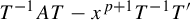 $T^{-1}AT-x^{p+1}T^{-1}T'$
belongs to
$T^{-1}AT-x^{p+1}T^{-1}T'$
belongs to
 $\mathcal {M}_n(\mathbb R[[x]])$
(this is always the case if
$\mathcal {M}_n(\mathbb R[[x]])$
(this is always the case if
 $\Psi _{T}$
is regular polynomial) or a ramification
$\Psi _{T}$
is regular polynomial) or a ramification
 $R_r$
and (S) is singular (
$R_r$
and (S) is singular (
 $p\ge 0$
). By extension, a composition of such transformations is admissible for a system
$p\ge 0$
). By extension, a composition of such transformations is admissible for a system
 $(S)$
if each transformation is admissible for the system to which it is applied.
$(S)$
if each transformation is admissible for the system to which it is applied.
To introduce the main result of [Reference Barkatou, Carnicero and Sanz Sánchez3], we need the following definition (recall the notation introduced in § 1.1 for the space
 $\mathbb R_k[x]$
of polynomials with degree at most k, as well as the definition and properties of the morphism
$\mathbb R_k[x]$
of polynomials with degree at most k, as well as the definition and properties of the morphism
 $\Theta $
).
$\Theta $
).
Definition 2.2. Let q be a non-negative integer. A system
 $x^{q+1}\boldsymbol {y}'=A(x)\cdot \boldsymbol {y}$
is said to be in TRS form of Poincaré rank q (or (TRS)
$x^{q+1}\boldsymbol {y}'=A(x)\cdot \boldsymbol {y}$
is said to be in TRS form of Poincaré rank q (or (TRS)
 $^q$
-form) if the matrix
$^q$
-form) if the matrix
 $A(x)$
is written as
$A(x)$
is written as
where:
-
(1)
$D\in \mathcal {M}_n(\mathbb R_{q-1}[x])$
is a polynomial matrix of degree at most
$q-1$
for which there are natural numbers
$n_1,n_2\in \mathbb N_{\ge 0}$
with
$n=2n_1+n_2$
such that
$D(x)$
decomposes as
$D(x)=\Theta (D_1(x))\oplus D_2(x)$
, with
$$ \begin{align*}\begin{array}{c} D_1(x) = \mathrm{diag}(\alpha_1(x),\ldots,\alpha_{n_1}(x)),{}\quad \alpha_j(x)\in\mathbb C_{q-1}[x]\text{ for all } j=1,\ldots,n_1,\\ D_2(x) = \mathrm{diag}(\beta_1(x),\ldots,\beta_{n_2}(x)),\quad \beta_j(x)\in \mathbb R_{q-1}[x]\text{ for all } j=1,\ldots,n_2;\\ \end{array}\end{align*} $$
-
(2)
$C\in \mathcal M_n(\mathbb R)$
is compatible with
$D(x)$
; -
(3)
$(D(x)+x^qC)_{|x=0}\neq 0$
(thus the system is singular and q is equal to its Poincaré rank); and -
(4)
$V(x)\in \mathcal {M}_{n}(\mathbb R[[x]])$
.


The matrix
 $D(x)+x^qC$
is called the principal part of the system,
$D(x)+x^qC$
is called the principal part of the system,
 $D(x)$
and C are called the exponential part and the residual part of the system, respectively, and
$D(x)$
and C are called the exponential part and the residual part of the system, respectively, and
 $V(x)$
is called the vestigial part of the system.
$V(x)$
is called the vestigial part of the system.
Remark 2.1. Definition 2.2 describes a system of
 $n=2n_1+n_2$
equations. The splitting between real and complex blocs is not necessarily unique, but we always assume that a given (TRS)
$n=2n_1+n_2$
equations. The splitting between real and complex blocs is not necessarily unique, but we always assume that a given (TRS)
 $^q$
-form of a system has a minimal
$^q$
-form of a system has a minimal
 $n_1$
. That is, for each
$n_1$
. That is, for each
 $j=1,\ldots ,n_1$
, at least one coefficient of the polynomial
$j=1,\ldots ,n_1$
, at least one coefficient of the polynomial
 $\alpha _j(x)$
is non-real.
$\alpha _j(x)$
is non-real.
Definition 2.3. Following the terminology introduced in [Reference Balser2], a constant matrix
 $C\in \mathcal {M}_{n}(\mathbb {R})$
is said to have good spectrum if it has no two eigenvalues (in
$C\in \mathcal {M}_{n}(\mathbb {R})$
is said to have good spectrum if it has no two eigenvalues (in
 $\mathbb C$
) that differ by a non-zero integer number.
$\mathbb C$
) that differ by a non-zero integer number.
The main result of [Reference Barkatou, Carnicero and Sanz Sánchez3] that we use is as follows.
Theorem 2.2. [Reference Barkatou, Carnicero and Sanz Sánchez3]
Consider a singular system
 $$ \begin{align*} (S)\;\;\;\;\;\;x^{p+1}{\mathbf{y}}'=A(x) \cdot {\mathbf{y}} \end{align*} $$
with
 $A(x)\in \mathcal {M}_{n}(\mathbb {R}[[x]])$
and
$A(x)\in \mathcal {M}_{n}(\mathbb {R}[[x]])$
and
 $A(0)\ne 0$
. Then there exist a ramification
$A(0)\ne 0$
. Then there exist a ramification
 $R_r$
and a finite composition
$R_r$
and a finite composition
 $\psi $
of admissible gauge transformations, either regular polynomial or diagonal monomial, according to the following.
$\psi $
of admissible gauge transformations, either regular polynomial or diagonal monomial, according to the following.
-
(i) The composition
$\psi \circ R_r$
transforms the system
$(S)$
into a system
$(\widetilde {S})$
that is either regular or in (TRS)
$^q$
-form for some
$q\in \mathbb {N}_{\ge 0}$
, with a residual part which has good spectrum. -
(ii) Assume that (S) is already in (TRS)
$^p$
-form and with a residual part with good spectrum. Then, for any
$N\ge 1$
, there exists a regular polynomial gauge transformation
$\Psi _{T_N}$
that transforms the system (S) into another system in (TRS)
$^p$
-form with the same principal part as (S) and a vestigial part V satisfying
$V(x)=O(x^N)$
.


2.2 Admissible transformations for vector fields along a formal curve
Let
 $a\in X$
be a point in a smooth manifold X of dimension
$a\in X$
be a point in a smooth manifold X of dimension
 $1+n$
, and let
$1+n$
, and let
 $(\xi ,\Gamma )$
be a couple made of a germ
$(\xi ,\Gamma )$
be a couple made of a germ
 $\xi $
of a
$\xi $
of a
 $C^{\infty }$
vector field at a or a formal vector field
$C^{\infty }$
vector field at a or a formal vector field
 $\xi $
at a and a non-singular formal curve
$\xi $
at a and a non-singular formal curve
 $\Gamma $
at a, invariant for
$\Gamma $
at a, invariant for
 $\xi $
and not contained in the formal singular locus of
$\xi $
and not contained in the formal singular locus of
 $\xi $
. We call such a couple an invariant couple, either smooth or formal according to the nature of
$\xi $
. We call such a couple an invariant couple, either smooth or formal according to the nature of
 $\xi $
, and smooth by default. We say that a system of coordinates
$\xi $
, and smooth by default. We say that a system of coordinates
 $(x,\boldsymbol {y} =(y_1,\ldots ,y_n))$
centered at a is adapted to
$(x,\boldsymbol {y} =(y_1,\ldots ,y_n))$
centered at a is adapted to
 $\Gamma $
if the tangent line of
$\Gamma $
if the tangent line of
 $\Gamma $
is transverse to the hyperplane
$\Gamma $
is transverse to the hyperplane
 ${x=0}$
. In such coordinates,
${x=0}$
. In such coordinates,
 $\Gamma $
can be parameterized by x. This means that there is a unique
$\Gamma $
can be parameterized by x. This means that there is a unique
 $\Gamma _{{\mathbf {y}}}=(\Gamma _{y_1},\cdots \Gamma _{y_n})\in (x\mathbb {R}[[x]])^n$
such that
$\Gamma _{{\mathbf {y}}}=(\Gamma _{y_1},\cdots \Gamma _{y_n})\in (x\mathbb {R}[[x]])^n$
such that
 $\Gamma $
is given by
$\Gamma $
is given by
 $\boldsymbol {y}=\Gamma _{{\mathbf {y}}}(x)$
. We also write
$\boldsymbol {y}=\Gamma _{{\mathbf {y}}}(x)$
. We also write
 ${\Gamma = (x,\Gamma _{{\mathbf {y}}}(x))}$
. An adapted system
${\Gamma = (x,\Gamma _{{\mathbf {y}}}(x))}$
. An adapted system
 $(x,{\mathbf {y}})$
is said to have contact order m with
$(x,{\mathbf {y}})$
is said to have contact order m with
 $\Gamma $
, for a given
$\Gamma $
, for a given
 $m\in \mathbb N$
, if
$m\in \mathbb N$
, if
 $\text {ord}_x(\Gamma _{\boldsymbol {y}})= m$
.
$\text {ord}_x(\Gamma _{\boldsymbol {y}})= m$
.
Remark 2.3. If
 $\xi _{|a}=0$
and
$\xi _{|a}=0$
and
 $(x,{\mathbf {y}})$
has contact at least m with
$(x,{\mathbf {y}})$
has contact at least m with
 $\Gamma $
, then
$\Gamma $
, then
 $$ \begin{align*}\text{ord}_x(\xi_{{\mathbf{y}}}(x,\boldsymbol{0}))\ge m,\end{align*} $$
where
 $\xi _{{\mathbf {y}}}=(\xi (y_1),\ldots ,\xi (y_n))$
. Indeed,
$\xi _{{\mathbf {y}}}=(\xi (y_1),\ldots ,\xi (y_n))$
. Indeed,
 $\Gamma $
being invariant,
$\Gamma $
being invariant,
 $\Gamma '\wedge \hat \xi \circ \Gamma =0$
, which gives, considering the terms in
$\Gamma '\wedge \hat \xi \circ \Gamma =0$
, which gives, considering the terms in
 $\partial _x\wedge \partial _{{\mathbf {y}}}$
,
$\partial _x\wedge \partial _{{\mathbf {y}}}$
,
 $$ \begin{align*}\hat\xi_{{\mathbf{y}}}(\Gamma) - \hat\xi_x(\Gamma)\Gamma_{{\mathbf{y}}}'=0.\end{align*} $$
But
 $\hat \xi _x(\Gamma )=O(x)$
since
$\hat \xi _x(\Gamma )=O(x)$
since
 $\xi _{|a}=0$
, and
$\xi _{|a}=0$
, and
 $\Gamma _{{\mathbf {y}}}'(x)=O(x^{m-1})$
, so
$\Gamma _{{\mathbf {y}}}'(x)=O(x^{m-1})$
, so
 $\hat \xi _{{\mathbf {y}}}(\Gamma )=O(x^m)$
. Now
$\hat \xi _{{\mathbf {y}}}(\Gamma )=O(x^m)$
. Now
 $\hat \xi _{{\mathbf {y}}}(x,\boldsymbol {0})= \hat \xi _{{\mathbf {y}}}(\Gamma ) - \partial _{{\mathbf {y}}} \hat \xi _{{\mathbf {y}}}(\Gamma )\cdot (\Gamma _{{\mathbf {y}}})+o(\Gamma _{{\mathbf {y}}})$
, and, since
$\hat \xi _{{\mathbf {y}}}(x,\boldsymbol {0})= \hat \xi _{{\mathbf {y}}}(\Gamma ) - \partial _{{\mathbf {y}}} \hat \xi _{{\mathbf {y}}}(\Gamma )\cdot (\Gamma _{{\mathbf {y}}})+o(\Gamma _{{\mathbf {y}}})$
, and, since
 $\Gamma _{{\mathbf {y}}}=O(x^m)$
, we get
$\Gamma _{{\mathbf {y}}}=O(x^m)$
, we get
 $\xi _{{\mathbf {y}}}(x,\boldsymbol {0}) = O(x^m)$
, as claimed.
$\xi _{{\mathbf {y}}}(x,\boldsymbol {0}) = O(x^m)$
, as claimed.
We define the transformations allowed for an invariant couple
 $(\xi ,\Gamma )$
.
$(\xi ,\Gamma )$
.
Definition 2.4. Let
 $(\xi , \Gamma )$
be a smooth (respectively, formal) invariant couple. An admissible transformation for
$(\xi , \Gamma )$
be a smooth (respectively, formal) invariant couple. An admissible transformation for
 $(\xi ,\Gamma )$
is a germ of a
$(\xi ,\Gamma )$
is a germ of a
 $C^{\infty }$
map
$C^{\infty }$
map
 $\phi :(Y,b)\to (X,a)$
, where Y is a smooth manifold of dimension
$\phi :(Y,b)\to (X,a)$
, where Y is a smooth manifold of dimension
 $1+n$
, of one of the following types.
$1+n$
, of one of the following types.
-
(i) Isomorphism.
$\phi $
is a germ of a
$C^{\infty }$
diffeomorphism. -
(ii) Blowing-up. There exists a germ
$(Z,a)\subset (X,a)$
of a smooth submanifold, which is (respectively, formally) invariant for
$\xi $
and not tangent to
$\Gamma $
at a, such that
$\phi $
is the germ at b of the blowing-up
$\pi _Z:Y\to X$
with center Z and
$b\in \pi _Z^{-1}(a)$
is the point corresponding to the tangent line of
$\Gamma $
. When
$Z=\{a\}$
, we say that
$\pi _Z$
is a punctual blowing-up. (See, for example, [Reference Hironaka14] or [Reference Bierstone and Milman4] for intrinsic definitions of blowing-ups). -
(iii) Ramification. There exists a system of adapted coordinates
$\tau =(x,{\mathbf {y}})$
for
$\Gamma $
such that the hyperplane
$H=\{x=0\}$
is (respectively, formally) invariant for
$\xi $
, and there exists some
$r\in \mathbb {N}_{>0}$
such that
$(Y,b)=(\mathbb {R}^{1+n},0)$
and
$\tau \circ \phi =R_r$
, where
$R_r$
is the map
$R_r(x,{\mathbf {y}})=(x^r,{\mathbf {y}})$
.


For each admissible transformation
 $\phi :(Y,b)\to (X,a)$
, the lift, or transformed couple
$\phi :(Y,b)\to (X,a)$
, the lift, or transformed couple
 $\phi ^*(\xi ,\Gamma )$
of
$\phi ^*(\xi ,\Gamma )$
of
 $(\xi ,\Gamma )$
by
$(\xi ,\Gamma )$
by
 $\phi $
is the couple
$\phi $
is the couple
 $(\widetilde {\xi },\widetilde {\Gamma })$
, where
$(\widetilde {\xi },\widetilde {\Gamma })$
, where
 $\widetilde {\xi }$
is the germ of a
$\widetilde {\xi }$
is the germ of a
 $C^{\infty }$
(respectively, formal) vector field at
$C^{\infty }$
(respectively, formal) vector field at
 $b\in Y$
satisfying
$b\in Y$
satisfying
 $\phi _*\widetilde {\xi }=\xi $
, and
$\phi _*\widetilde {\xi }=\xi $
, and
 $\widetilde {\Gamma }$
is the non-singular formal curve satisfying
$\widetilde {\Gamma }$
is the non-singular formal curve satisfying
 $\widehat \phi (\widetilde {\Gamma })=\Gamma $
. The invariance conditions ensure that
$\widehat \phi (\widetilde {\Gamma })=\Gamma $
. The invariance conditions ensure that
 $\widetilde {\xi }$
exists as a smooth (respectively, formal) vector field, and the condition on b for the blowing-up ensures that
$\widetilde {\xi }$
exists as a smooth (respectively, formal) vector field, and the condition on b for the blowing-up ensures that
 $\widetilde {\Gamma }$
is a formal curve at b. Noticeably,
$\widetilde {\Gamma }$
is a formal curve at b. Noticeably,
 $(\widetilde {\xi }, \widetilde {\Gamma })$
is an invariant couple again. Iterating, the lift of
$(\widetilde {\xi }, \widetilde {\Gamma })$
is an invariant couple again. Iterating, the lift of
 $(\xi ,\Gamma )$
by a finite composition of admissible transformations
$(\xi ,\Gamma )$
by a finite composition of admissible transformations
 $\psi =\phi _r\circ \cdots \circ \phi _1$
refers to
$\psi =\phi _r\circ \cdots \circ \phi _1$
refers to
 $\psi ^*(\xi ,\Gamma )=\phi _1^*\phi _{2}^*\cdots \phi _r^*(\xi ,\Gamma )$
.
$\psi ^*(\xi ,\Gamma )=\phi _1^*\phi _{2}^*\cdots \phi _r^*(\xi ,\Gamma )$
.
The (TRS)-form that we provide below for an invariant couple
 $(\xi ,\Gamma )$
is a practical expression of
$(\xi ,\Gamma )$
is a practical expression of
 $\xi $
in some coordinates adapted to
$\xi $
in some coordinates adapted to
 $\Gamma $
, so we often need to reason with particular coordinate systems. For this, we list below the coordinate systems and change of coordinates we use and the effect of the admissible transformations on the coordinates of
$\Gamma $
, so we often need to reason with particular coordinate systems. For this, we list below the coordinate systems and change of coordinates we use and the effect of the admissible transformations on the coordinates of
 $(\xi ,\Gamma )$
.
$(\xi ,\Gamma )$
.
Definition 2.5. Let
 $(\xi ,\Gamma )$
be a a smooth (respectively, formal) invariant couple, and let
$(\xi ,\Gamma )$
be a a smooth (respectively, formal) invariant couple, and let
 $(x,\boldsymbol {y})$
be an adapted coordinate system. An admissible coordinate transformation for
$(x,\boldsymbol {y})$
be an adapted coordinate system. An admissible coordinate transformation for
 $(\xi ,\Gamma , (x,\boldsymbol {y}))$
is a germ of a
$(\xi ,\Gamma , (x,\boldsymbol {y}))$
is a germ of a
 $C^{\infty }$
map
$C^{\infty }$
map
 $\phi :(\mathbb R^{1+n},0)\ni (x, {\mathbf {y}})\mapsto (\widetilde {x},\widetilde {{\mathbf {y}}}) \in (\mathbb R^{1+n},0)$
, (respectively, a formal map
$\phi :(\mathbb R^{1+n},0)\ni (x, {\mathbf {y}})\mapsto (\widetilde {x},\widetilde {{\mathbf {y}}}) \in (\mathbb R^{1+n},0)$
, (respectively, a formal map
 $(\widetilde {x}, \boldsymbol {\widetilde {y}})=\phi (x,\boldsymbol {y})\in \mathbb R[[x,{{\mathbf {y}}}]]^{1+n}$
) of the following types. (For each type, we give the expression of the transformed couple
$(\widetilde {x}, \boldsymbol {\widetilde {y}})=\phi (x,\boldsymbol {y})\in \mathbb R[[x,{{\mathbf {y}}}]]^{1+n}$
) of the following types. (For each type, we give the expression of the transformed couple
 $(\widetilde {\xi },\widetilde {\Gamma })=\phi ^*(\xi ,\Gamma )$
in the coordinate system
$(\widetilde {\xi },\widetilde {\Gamma })=\phi ^*(\xi ,\Gamma )$
in the coordinate system
 $(\widetilde {x}, \widetilde {\boldsymbol {y}})$
.)
$(\widetilde {x}, \widetilde {\boldsymbol {y}})$
.)
-
(1) Affine polynomial. This regroups the following two types of transformations.
-
(a) Polynomial translation. A map of the form
where
$$ \begin{align*} (x,{\mathbf{y}})=T_{\boldsymbol{\beta}}(\widetilde{x},\widetilde{{\mathbf{y}}}):= (\widetilde{x},\boldsymbol{\beta}(\widetilde{x})+\widetilde{{\mathbf{y}}}), \end{align*} $$
${\boldsymbol {\beta }}(\widetilde {x})\in (x\mathbb {R}[\widetilde {x}])^{n}$
. In coordinates, we get
$$ \begin{align*} \widetilde{\xi} & = \xi_x\circ\phi\; \partial_{\widetilde{x}}+(\xi_{{\mathbf{y}}}\circ\phi\;-(\xi_x\circ\phi)\; {\boldsymbol{\beta}}'(\widetilde{x}))\cdot \partial_{\widetilde{\boldsymbol{y}}},\\ \widetilde{\Gamma} & = (\widetilde{x}, \Gamma_{\boldsymbol{y}}(\widetilde{x}) -{\boldsymbol{\beta}}(\widetilde{x})). \end{align*} $$
-
(b) Polynomial regular. Any map of the form
where
$$ \begin{align*} (x,{\mathbf{y}})=\Psi_{P}(\widetilde{x},\widetilde{{\mathbf{y}}}):=(\widetilde{x}, P(\widetilde{x})\cdot \widetilde{{\mathbf{y}}}), \end{align*} $$
$P(\widetilde {x})\in \mathcal {M}_{n}(\mathbb {R}[\widetilde {x}])$
and
$P(0)\in \text {GL}_n(\mathbb R)$
. In coordinates, we get (
$$ \begin{align*} \widetilde{\xi} & = \xi_x\circ\phi\; \partial_{\widetilde{x}}+(P^{-1}(\widetilde{x}) \cdot \xi_{{\mathbf{y}}}\circ\phi\;-(\xi_x\circ\phi)\,{P^{-1}(\widetilde{x}) \cdot} P'(\widetilde{x})\cdot\widetilde{{\mathbf{y}}})\cdot \partial_{\widetilde{\boldsymbol{y}}},\\ \widetilde{\Gamma} & = (\widetilde{x}, P^{-1}(\widetilde{x}) \cdot \Gamma_{\boldsymbol{y}}(\widetilde{x})). \end{align*} $$
$P(0)\in \text {GL}_n(\mathbb R)$
implies that
$P^{-1}$
exists in
$\mathcal {M}_n(C^{\infty }(\mathbb R))$
and in
$\mathcal {M}_n(\mathbb R[[x]])$
).
-
-
(2) Diagonal monomial. A map
$\phi $
of the form
$(x,\boldsymbol {y}) = (\widetilde {x}, ((\widetilde {x} I_k) \oplus I_{n-k}) \cdot \widetilde {{\mathbf {y}}})$
, with
${1\le k \le n}$
, admissible if
$(x,{\mathbf {y}})$
has contact order at least two with
$\Gamma $
and the center
${\{x=0,{\mathbf {y}}_1=\boldsymbol {0}\}}$
is invariant by
$\xi $
, where
${\mathbf {y}}_1=(y_1,\ldots ,y_k)$
. In this case, writing also
${\mathbf {y}}_2=(y_{k+1},\ldots ,y_{n}),\; \widetilde {\mathbf {y}}_1=(\widetilde {y}_1,\ldots ,\widetilde {y}_k),\; \widetilde {{\mathbf {y}}}_2=(\widetilde {y}_{k+1},\ldots ,\widetilde {y}_n)$
, When
$$ \begin{align*} \widetilde{\xi} &=(\xi_x\circ\phi)\; \partial_{\widetilde{x}}+\frac{1}{\widetilde{x}}\, (\xi_{{\mathbf{y}}_1}\circ\phi - (\xi_x\circ\phi)\;\widetilde{{\mathbf{y}}}_1) \cdot \partial_{\widetilde{{\mathbf{y}}}_1} + (\xi_{{\mathbf{y}}_2}\circ\phi)\cdot\partial_{\widetilde{{\mathbf{y}}}_2},\\ \widetilde{\Gamma} & = \bigg(\widetilde x, \frac{1}{\widetilde{x}}\Gamma_{{\mathbf{y}}_1}(\widetilde{x}),\Gamma_{{\mathbf{y}}_2}(\widetilde{x})\bigg). \end{align*} $$
$k=n$
, we say that the transformation is full diagonal monomial.
-
(3) Ramifications. A map
$\phi $
of the form
$(x,{\mathbf {y}})=(\widetilde {x}^r, \widetilde {{\mathbf {y}}})$
, where
$r\in \mathbb N_{>1}$
, is admissible if the hypersurface
$\{x=0\}$
is invariant by
$\xi $
. In this case, we have
$$ \begin{align*} \widetilde{\xi} & = \frac{1}{r}\; \widetilde{x}^{1-r}(\xi_x\circ\phi) \; \partial_{\widetilde{x}} + (\xi_{{\mathbf{y}}}\circ\phi) \cdot \partial_{\widetilde{{\mathbf{y}}}}, \\ \widetilde{\Gamma} & = (\widetilde{x}, \Gamma_{{\mathbf{y}}}(\widetilde{x}^r )). \end{align*} $$


The different notions of admissible transformations so introduced are closely linked. It is clear that an admissible coordinate transformation for
 $(\xi ,\Gamma ,(x,{\mathbf {y}}))$
is the expression in adapted coordinates of an admissible transformation of
$(\xi ,\Gamma ,(x,{\mathbf {y}}))$
is the expression in adapted coordinates of an admissible transformation of
 $(\xi ,\Gamma )$
. Affine polynomial transformations are isomorphisms. A diagonal monomial transformation is the expression in coordinates of the blowing-up of the invariant center
$(\xi ,\Gamma )$
. Affine polynomial transformations are isomorphisms. A diagonal monomial transformation is the expression in coordinates of the blowing-up of the invariant center
 $\{(x,{\mathbf {y}}_1)=0\}$
, and the contact order condition of
$\{(x,{\mathbf {y}}_1)=0\}$
, and the contact order condition of
 $(x,{\mathbf {y}})$
with
$(x,{\mathbf {y}})$
with
 $\Gamma $
implies that the point
$\Gamma $
implies that the point
 $(\widetilde {x},\widetilde {{\mathbf {y}}}) =0$
corresponds to the tangent line of
$(\widetilde {x},\widetilde {{\mathbf {y}}}) =0$
corresponds to the tangent line of
 $\Gamma $
. The definition of the ramification as a coordinate transformation coincides with the one as admissible for the couple
$\Gamma $
. The definition of the ramification as a coordinate transformation coincides with the one as admissible for the couple
 $(\xi ,\Gamma )$
.
$(\xi ,\Gamma )$
.
On the another hand, the gauge transformations and ramifications that are admissible for a formal linear system
 $x^{p+1}{\mathbf {y}}'=A(x)\cdot {\mathbf {y}}$
correspond to compositions of admissible coordinate transformations for
$x^{p+1}{\mathbf {y}}'=A(x)\cdot {\mathbf {y}}$
correspond to compositions of admissible coordinate transformations for
 $(\xi ,\Gamma ,(x,{\mathbf {y}}))$
with
$(\xi ,\Gamma ,(x,{\mathbf {y}}))$
with
 $\xi = x^{p+1}\partial _x+(A(x)\cdot {\mathbf {y}})\cdot \partial _{{\mathbf {y}}}$
and
$\xi = x^{p+1}\partial _x+(A(x)\cdot {\mathbf {y}})\cdot \partial _{{\mathbf {y}}}$
and
 ${\Gamma = (x,\boldsymbol {0})}$
. This is checked directly by the definition for affine polynomial transformations or ramifications. For diagonal monomial transformations, we need the following proposition that ensures that the property of admissibility for this kind of vector field is the same as admissibility for the linear systems that they represent.
${\Gamma = (x,\boldsymbol {0})}$
. This is checked directly by the definition for affine polynomial transformations or ramifications. For diagonal monomial transformations, we need the following proposition that ensures that the property of admissibility for this kind of vector field is the same as admissibility for the linear systems that they represent.
Proposition 2.4. Let
 $\Psi _T$
be a diagonal monomial transformation admissible for the system
$\Psi _T$
be a diagonal monomial transformation admissible for the system
 $(S):\; x^{p+1}{\mathbf {y}}'=A(x)\cdot {\mathbf {y}}$
, let
$(S):\; x^{p+1}{\mathbf {y}}'=A(x)\cdot {\mathbf {y}}$
, let
 $(\widetilde {S}):\; x^{q+1}{\mathbf {y}}'=B(x)\cdot {\mathbf {y}}$
be the transformed system, let
$(\widetilde {S}):\; x^{q+1}{\mathbf {y}}'=B(x)\cdot {\mathbf {y}}$
be the transformed system, let
 $\xi = x^{p+1}\partial _x +(A(x)\cdot {\mathbf {y}})\cdot \partial _{{\mathbf {y}}}$
and let
$\xi = x^{p+1}\partial _x +(A(x)\cdot {\mathbf {y}})\cdot \partial _{{\mathbf {y}}}$
and let
 $\Gamma =(x,\boldsymbol {0})$
. Then there exist a composition of diagonal monomial coordinate transformations
$\Gamma =(x,\boldsymbol {0})$
. Then there exist a composition of diagonal monomial coordinate transformations
 $\Phi $
admissible for
$\Phi $
admissible for
 $(\xi ,\Gamma ,(x,{\mathbf {y}}))$
such that
$(\xi ,\Gamma ,(x,{\mathbf {y}}))$
such that
 $$ \begin{align*} \Phi^*(\xi,\Gamma,(x,{\mathbf{y}}))=(x^{q+1}\partial_{x} +(B(x)\cdot\widetilde{{\mathbf{y}}})\cdot\partial_{\widetilde{{\mathbf{y}}}},(x,\boldsymbol{0}),(x, \widetilde{{\mathbf{y}}})). \end{align*} $$
Proof. We write
 $T=\text {Diag}(x^{k_1}I_{n_1},\ldots ,x^{k_m}I_{n_m})$
with
$T=\text {Diag}(x^{k_1}I_{n_1},\ldots ,x^{k_m}I_{n_m})$
with
 $k_1>k_2>\cdots >k_m$
and
$k_1>k_2>\cdots >k_m$
and
 ${n_1+\cdots +n_m=n}$
after gathering the exponents that coincide and eventually permuting the variables. Remark that T is the product
${n_1+\cdots +n_m=n}$
after gathering the exponents that coincide and eventually permuting the variables. Remark that T is the product
 $$ \begin{align*}T = T_1^{k_1-k_2}\cdot T_2^{k_2-k_3}{\cdot} \;\cdots\; {\cdot} T_m^{k_m},\end{align*} $$
where
 $T_m=xI_n$
, and, for
$T_m=xI_n$
, and, for
 $i<m$
,
$i<m$
,
 $T_i = xI_{n_1+\cdots +n_i}\oplus I_{n_{i+1}+\cdots +n_m}$
. On the level of gauge transformations, this gives
$T_i = xI_{n_1+\cdots +n_i}\oplus I_{n_{i+1}+\cdots +n_m}$
. On the level of gauge transformations, this gives
 $\Psi _{T}=\Psi _{T_m}^{(m)}\circ \cdots \circ \Psi _{T_1}^{(k_1-k_2)}$
, where powers are compositions. Now, from their expressions in coordinates, the
$\Psi _{T}=\Psi _{T_m}^{(m)}\circ \cdots \circ \Psi _{T_1}^{(k_1-k_2)}$
, where powers are compositions. Now, from their expressions in coordinates, the
 $\Psi _{T_i}$
act on a system in the same way as the diagonal monomial coordinate transformation
$\Psi _{T_i}$
act on a system in the same way as the diagonal monomial coordinate transformation
 $\Phi _{T_i}(x, \widetilde {y}) = (x, T_i(x)\cdot \widetilde {y})$
acts on the corresponding vector field. So
$\Phi _{T_i}(x, \widetilde {y}) = (x, T_i(x)\cdot \widetilde {y})$
acts on the corresponding vector field. So
 $\Phi = \Phi _{T_m}^{(m)}\circ \cdots \circ \Phi _{T_1}^{(k_1-k_2)}$
solves the problem, up to checking that it is admissible.
$\Phi = \Phi _{T_m}^{(m)}\circ \cdots \circ \Phi _{T_1}^{(k_1-k_2)}$
solves the problem, up to checking that it is admissible.
We investigate the admissibility condition on a generic case shaped as the
 $T_i$
, say,
$T_i$
, say,
 ${G=xI_{\ell }\oplus I_{n-\ell }}$
. We decompose A by blocks of sizes
${G=xI_{\ell }\oplus I_{n-\ell }}$
. We decompose A by blocks of sizes
 $\ell $
and
$\ell $
and
 $n-\ell $
as
$n-\ell $
as
 $$ \begin{align*} A=\begin{pmatrix} A_{11} & A_{12}\\ A_{21} & A_{22} \end{pmatrix},\; A_{11}\in\mathcal M_{\ell}(\mathbb R[[x]]),\; A_{22}\in\mathcal M_{n-\ell}(\mathbb R[[x]]). \end{align*} $$
Then
 $$ \begin{align*} G^{-1}\cdot A\cdot G-x^{p+1}G^{-1}\cdot G' = \begin{pmatrix}A_{11} -x^pI_{\ell} & x^{-1}A_{12}\\ xA_{21} & A_{22}\end{pmatrix}, \end{align*} $$
and we see that
 $\Psi _G$
is admissible for (S) if and only if x divides
$\Psi _G$
is admissible for (S) if and only if x divides
 $A_{12}$
.
$A_{12}$
.
Since the order of the coefficients above the diagonal cannot increase by iterating such types of transformations, we get that
 $\Psi _T$
is admissible for
$\Psi _T$
is admissible for
 $(S)$
if and only if
$(S)$
if and only if
 $\Psi _{T_1}$
is admissible for
$\Psi _{T_1}$
is admissible for
 $(S)$
and
$(S)$
and
 $\Psi _{\check {T}}$
is admissible for the system transformed by
$\Psi _{\check {T}}$
is admissible for the system transformed by
 $\Psi _{T_1}$
, where
$\Psi _{T_1}$
, where
 $\check T = T_1^{k_1-k_2-1}\cdot T_2^{k_2-k_3}{\cdot } \cdots {\cdot } T_m^{k_m}$
. So we only need to prove that the admissibility of
$\check T = T_1^{k_1-k_2-1}\cdot T_2^{k_2-k_3}{\cdot } \cdots {\cdot } T_m^{k_m}$
. So we only need to prove that the admissibility of
 $\Phi _{T_1}$
follows from the admissibility of
$\Phi _{T_1}$
follows from the admissibility of
 $\Psi _{T_1}$
.
$\Psi _{T_1}$
.
From the calculation above,
 $\Psi _{T_1}$
is admissible for
$\Psi _{T_1}$
is admissible for
 $(S)$
means that
$(S)$
means that
 $A_{12}(0)=0$
. Write
$A_{12}(0)=0$
. Write
 ${\mathbf {y}}_1=(y_1,\ldots ,y_{n_1}), {\mathbf {y}}_2=(y_{n_1+1},\ldots , {\mathbf {y}}_n)$
, so
${\mathbf {y}}_1=(y_1,\ldots ,y_{n_1}), {\mathbf {y}}_2=(y_{n_1+1},\ldots , {\mathbf {y}}_n)$
, so
 $$ \begin{align*}\xi = x^{p+1}\partial_x + (A_{11}\cdot {\mathbf{y}}_1+A_{12}\cdot {\mathbf{y}}_2)\cdot\partial_{{\mathbf{y}}_1}+(A_{21}\cdot{\mathbf{y}}_1+ A_{22}\cdot {\mathbf{y}}_2)\cdot\partial_{{\mathbf{y}}_2}.\end{align*} $$
The restriction of
 $\xi $
to the center
$\xi $
to the center
 $\{x=0, {\mathbf {y}}_1=0\}$
is given by
$\{x=0, {\mathbf {y}}_1=0\}$
is given by
 $$ \begin{align*}\xi\circ(0,\boldsymbol{0},{\mathbf{y}}_2) = (A_{12}(0)\cdot {\mathbf{y}}_2)\cdot\partial_{{\mathbf{y}}_1}+( A_{22}(0)\cdot {\mathbf{y}}_2)\cdot\partial_{{\mathbf{y}}_2},\end{align*} $$
and since
 $A_{12}(0)$
vanishes if
$A_{12}(0)$
vanishes if
 $\Psi _{T_1}$
is admissible, we see that this restriction belongs to
$\Psi _{T_1}$
is admissible, we see that this restriction belongs to
 $\text {Span}(\partial _{{\mathbf {y}}_2})=\text {ker}(dx\wedge dy_1\wedge \cdots \wedge dy_{n_1})$
. In other words,
$\text {Span}(\partial _{{\mathbf {y}}_2})=\text {ker}(dx\wedge dy_1\wedge \cdots \wedge dy_{n_1})$
. In other words,
 $\{x=0, {\mathbf {y}}_1=\boldsymbol {0}\}$
is invariant by
$\{x=0, {\mathbf {y}}_1=\boldsymbol {0}\}$
is invariant by
 $\xi $
. Therefore
$\xi $
. Therefore
 $\Phi _{T_1}$
is admissible, as required.
$\Phi _{T_1}$
is admissible, as required.
Full diagonal monomial transformations (punctual blowing-ups) play an important role in our reduction. We detail here a property of divisibility by the equation of the exceptional divisor that we use several times in what follows.
Lemma 2.5. Let
 $(\xi ,\Gamma )$
be a smooth invariant couple, let
$(\xi ,\Gamma )$
be a smooth invariant couple, let
 $(x,{\mathbf {y}})$
be a system of adapted coordinates, let
$(x,{\mathbf {y}})$
be a system of adapted coordinates, let
 $k\in \mathbb N$
and let
$k\in \mathbb N$
and let
 $\phi $
be the full diagonal monomial transformation. Suppose
$\phi $
be the full diagonal monomial transformation. Suppose
 $\xi |_0=0$
and set
$\xi |_0=0$
and set
 $(\zeta ,\Delta ,(x,{\mathbf {z}}))=\phi ^*(\xi ,\Gamma , (x,{\mathbf {y}}))$
. Then
$(\zeta ,\Delta ,(x,{\mathbf {z}}))=\phi ^*(\xi ,\Gamma , (x,{\mathbf {y}}))$
. Then
 $x^{k}$
divides
$x^{k}$
divides
 $\widehat {\zeta }_{{\mathbf {z}}}$
(respectively,
$\widehat {\zeta }_{{\mathbf {z}}}$
(respectively,
 $\widehat {\zeta }_x$
) if and only if
$\widehat {\zeta }_x$
) if and only if
 $x^{k}$
divides
$x^{k}$
divides
 $\zeta _{{\mathbf {z}}}$
(respectively,
$\zeta _{{\mathbf {z}}}$
(respectively,
 $\zeta _x$
) in
$\zeta _x$
) in
 $C^{\infty }(\mathbb R^{1+n},0)$
.
$C^{\infty }(\mathbb R^{1+n},0)$
.
Proof. The direct implication is not obvious. We have
 $x\zeta _{{\mathbf {z}}}(x,{\mathbf {z}})=\xi _{{\mathbf {y}}}(x,x{\mathbf {z}})-\xi _x(x,x{\mathbf {z}}){\mathbf {z}}$
, and
$x\zeta _{{\mathbf {z}}}(x,{\mathbf {z}})=\xi _{{\mathbf {y}}}(x,x{\mathbf {z}})-\xi _x(x,x{\mathbf {z}}){\mathbf {z}}$
, and
 $\zeta _x(x,{\mathbf {z}}) = \xi _x(x,x{\mathbf {z}})$
. The proof for both is analogous, so we focus on
$\zeta _x(x,{\mathbf {z}}) = \xi _x(x,x{\mathbf {z}})$
. The proof for both is analogous, so we focus on
 $\zeta _{{\mathbf {z}}}$
. We write the Taylor expansion with integral remainder for
$\zeta _{{\mathbf {z}}}$
. We write the Taylor expansion with integral remainder for
 $\varphi :t\mapsto \xi _{{\mathbf {y}}}(t(x,x{\mathbf {z}}))-\xi _x(t(x,x{\mathbf {z}})){\mathbf {z}}$
between
$\varphi :t\mapsto \xi _{{\mathbf {y}}}(t(x,x{\mathbf {z}}))-\xi _x(t(x,x{\mathbf {z}})){\mathbf {z}}$
between
 $t=0$
and
$t=0$
and
 $t=1$
: that is,
$t=1$
: that is,
 $$ \begin{align*} & x\,\zeta_{{\mathbf{z}}}(x,{\mathbf{z}})\\ & \quad=\varphi(1) = \sum_{m=0}^k\frac{1}{m!} (d^{m}\xi_{{\mathbf{y}}}(0,0)((x,x{\mathbf{z}})^{(m)})-d^{m}\xi_x(0,0)((x,x{\mathbf{z}})^{(m)}){\mathbf{z}}) \cdots\\ &\qquad + \int_0^1( d^{k+1}\xi_{{\mathbf{y}}}(t(x,x{\mathbf{z}}))((x,x{\mathbf{z}})^{(k+1)})-d^{k+1}\xi_x(t(x,x{\mathbf{z}}))((x,x{\mathbf{z}})^{(k+1)}){\mathbf{z}}) \frac{(1-t)^k \;dt}{k!} \\ & \quad = \sum_{m=0}^k\frac{x^m}{m!} (d^{m}\xi_{{\mathbf{y}}}(0,0)((1,{\mathbf{z}})^{(m)})-d^{m}\xi_x(0,0)((1,{\mathbf{z}})^{(m)}){\mathbf{z}})\cdots \\ & \qquad + x^{k+1}\!\int_0^1\!( d^{k+1}\xi_{{\mathbf{y}}}(t(x,x{\mathbf{z}}))((1,{\mathbf{z}})^{(k+1)})-d^{k+1}\xi_x(t(x,x{\mathbf{z}}))((1,{\mathbf{z}})^{(k+1)}){\mathbf{z}}) \frac{(1-t)^k dt}{k!}. \end{align*} $$
In the last expression, the integral is
 $C^{\infty }$
(in terms of
$C^{\infty }$
(in terms of
 $(x,{\mathbf {z}})$
) by the Leibniz integral rule, so
$(x,{\mathbf {z}})$
) by the Leibniz integral rule, so
 $x^{k+1}$
divides the remainder. The initial sum is a polynomial, of degree k in x. The formal divisibility of the left-hand side by
$x^{k+1}$
divides the remainder. The initial sum is a polynomial, of degree k in x. The formal divisibility of the left-hand side by
 $x^{k+1}$
implies that this polynomial is identically zero. Thus
$x^{k+1}$
implies that this polynomial is identically zero. Thus
 $\zeta _{{\mathbf {z}}}(x,{\mathbf {z}})=x^{k} f(x,{\mathbf {z}})$
, where f is the parametric integral.
$\zeta _{{\mathbf {z}}}(x,{\mathbf {z}})=x^{k} f(x,{\mathbf {z}})$
, where f is the parametric integral.
2.3 Reduction of a vector field to (TRS)-form along an invariant curve
As in the preceding paragraph,
 $(\xi ,\Gamma )$
is an invariant couple.
$(\xi ,\Gamma )$
is an invariant couple.
Definition 2.6. Let
 $q\in \mathbb N$
be a non-negative integer. We say that the vector field
$q\in \mathbb N$
be a non-negative integer. We say that the vector field
 $\xi $
is in (TRS)-form of type
$\xi $
is in (TRS)-form of type
 $(q,N,M)$
if there exists a system of coordinates
$(q,N,M)$
if there exists a system of coordinates
 $(x,{\mathbf {y}}):(X,a)\to \mathbb R^{1+n}$
, such that
$(x,{\mathbf {y}}):(X,a)\to \mathbb R^{1+n}$
, such that
 $$ \begin{align} \xi=x^e u(x,{\mathbf{y}})[x^{q+1}\partial_x+( (D(x)+x^qC )\cdot{\mathbf{y}}+x^{q+1+N}V(x,x^M{\mathbf{y}}))\cdot\partial_{{\mathbf{y}}}], \end{align} $$
where
 $e\in \mathbb N$
,
$e\in \mathbb N$
,
 $u(x,{\mathbf {y}})$
is a germ of a
$u(x,{\mathbf {y}})$
is a germ of a
 $C^{\infty }$
unit,
$C^{\infty }$
unit,
 $D(x)$
and C satisfy conditions (1)–(3) of Definition 2.2 and
$D(x)$
and C satisfy conditions (1)–(3) of Definition 2.2 and
 $V:(\mathbb R^{1+n},0)\to \mathbb R^n$
is a map germ. We say that
$V:(\mathbb R^{1+n},0)\to \mathbb R^n$
is a map germ. We say that
 $(x,{\mathbf {y}})$
is a system of (TRS)-coordinates for
$(x,{\mathbf {y}})$
is a system of (TRS)-coordinates for
 $\xi $
. The terms
$\xi $
. The terms
 $D(x)$
, C and
$D(x)$
, C and
 $V(x,{\mathbf {y}})$
are, respectively, called the exponential part, the residual part and the vestigial part of the (TRS)-form. If
$V(x,{\mathbf {y}})$
are, respectively, called the exponential part, the residual part and the vestigial part of the (TRS)-form. If
 $(\xi ,\Gamma )$
is an invariant couple and
$(\xi ,\Gamma )$
is an invariant couple and
 $(x,{\mathbf {y}})$
is system of (TRS)-coordinates for
$(x,{\mathbf {y}})$
is system of (TRS)-coordinates for
 $\xi $
that is adapted to
$\xi $
that is adapted to
 $\Gamma $
, we say that the couple
$\Gamma $
, we say that the couple
 $(\xi ,\Gamma )$
admits a (TRS)-form, with (TRS)-coordinates
$(\xi ,\Gamma )$
admits a (TRS)-form, with (TRS)-coordinates
 $(x,{\mathbf {y}})$
; or, for simplicity, that
$(x,{\mathbf {y}})$
; or, for simplicity, that
 $(\xi ,\Gamma ,(x,{\mathbf {y}}))$
is in (TRS)-form (of the corresponding type).
$(\xi ,\Gamma ,(x,{\mathbf {y}}))$
is in (TRS)-form (of the corresponding type).
The main result in this section establishes that any invariant couple
 $(\xi ,\Gamma )$
can be reduced to (TRS)-form after finitely many admissible transformations.
$(\xi ,\Gamma )$
can be reduced to (TRS)-form after finitely many admissible transformations.
Theorem 2.6. Let
 $(\xi ,\Gamma )$
be an invariant couple at
$(\xi ,\Gamma )$
be an invariant couple at
 $(X,a)$
and assume that
$(X,a)$
and assume that
 $\xi |_a=0$
.
$\xi |_a=0$
.
-
(i) There exists
$q\in \mathbb N$
and a finite composition
$\psi :(Y,b)\to (X,a)$
of admissible transformations for
$(\xi ,\Gamma )$
such that the transformed couple
$(\widetilde {\xi },\widetilde {\Gamma })=\psi ^*(\xi ,\Gamma )$
admits a (TRS)-form of type
$(q,0,0)$
, with a
$C^{\infty }$
vestigial part and a residual part with a good spectrum. Precisely, for all systems of coordinates
$(x,{\mathbf {y}})$
at
$(X,a)$
adapted to
$(\xi ,\Gamma )$
, there exists a system of (TRS)-coordinates
$(\widetilde {x}, \widetilde {{\mathbf {y}}})$
at
$(Y,b)$
for
$\psi ^*(\xi ,\Gamma )$
, and a finite composition of admissible coordinate transformations
$\Psi $
such that
$\Psi ^*(\xi ,\Gamma ,(x,{\mathbf {y}}))=(\psi ^*(\xi ,\Gamma ),(\widetilde {x},\widetilde {{\mathbf {y}}}))$
. -
(ii) Let
$(\xi ,\Gamma )$
be an invariant couple at
$(Y,b)$
, with (TRS)-coordinates
$(x,{\mathbf {y}})$
of type
$(q,0,0)$
, a
$C^{\infty }$
vestigial part and a residual part with a good spectrum. Given
$N,M\ge 0$
, there exists a finite composition
$\psi _{N,M}:(W,c)\to (Y,b)$
of punctual blowing-ups such that
$(\widetilde {\xi },\widetilde {\Gamma }) : =(\psi _{N,M})^*(\xi ,\Gamma )$
admits a (TRS)-form of type
$(q,N,M)$
, with a
$C^{\infty }$
vestigial part. More precisely, there exist a system of (TRS)-coordinates
$(\widetilde {x},\widetilde {{\mathbf {y}}})$
for
$(\widetilde {\xi },\widetilde {\Gamma })$
and a finite composition
$\Psi _{N,M}$
of admissible coordinate transformations, made of affine polynomial and full diagonal monomial transformations, such that where
$$ \begin{align*} (\Psi_{N,M})^*(\xi,\Gamma,(x, {\mathbf{y}})) = (\widetilde{\xi},\widetilde{\Gamma},(\widetilde{x},\widetilde{{\mathbf{y}}})), \end{align*} $$
$(\widetilde {\xi },\widetilde {\Gamma },(\widetilde {x},\widetilde {{\mathbf {y}}}))$
has the same exponential part as
$(\xi ,\Gamma ,(x,{\mathbf {y}}))$
and a residual part with good spectrum included in
$\mathbb R^*_{-}\times i\mathbb R$
.


Remark 2.7. In addition to its use in the present paper, the theorem above has its own independent interest. In particular, it is a useful tool for studying the local dynamics of an analytic vector field. For this, we emphasis that, if
 $\xi $
is analytic, the following proof works step by step (with some eventual simplifications owing to the fact that formal divisibility implies analytic divisibility) and it shows a stronger form of reduction: only analytic admissible coordinate transformations are needed (the centers of the blowing-ups are smooth analytic manifolds). We chose to present here a proof that works directly in the analytic framework to use Theorem 2.6 for other purposes. The proof in the
$\xi $
is analytic, the following proof works step by step (with some eventual simplifications owing to the fact that formal divisibility implies analytic divisibility) and it shows a stronger form of reduction: only analytic admissible coordinate transformations are needed (the centers of the blowing-ups are smooth analytic manifolds). We chose to present here a proof that works directly in the analytic framework to use Theorem 2.6 for other purposes. The proof in the
 $C^\infty $
case could be shortened by starting with a system of coordinates
$C^\infty $
case could be shortened by starting with a system of coordinates
 $(x,{\mathbf {y}})$
having flat contact with the formal curve
$(x,{\mathbf {y}})$
having flat contact with the formal curve
 $\Gamma $
(that is,
$\Gamma $
(that is,
 $\Gamma _{{\mathbf {y}}}=0$
).
$\Gamma _{{\mathbf {y}}}=0$
).
2.4 Proof of Theorem 2.6
We fix initial adapted coordinates
 $(x,{\mathbf {y}})$
at the point
$(x,{\mathbf {y}})$
at the point
 $a\in X$
and write
$a\in X$
and write
 $$ \begin{align*} \xi= \xi_x\partial_x+\xi_{{\mathbf{y}}}\cdot\partial_{{\mathbf{y}}} \quad\text{and}\quad \Gamma=(x,\Gamma_{{\mathbf{y}}}(x)). \end{align*} $$
We consider several admissible coordinate transformations, starting from
 $(x,{\mathbf {y}})$
, to get to a system of (TRS)-coordinates. To lighten the notation, we do not systematically change the name of the different objects after each transformation, and we recycle old names when it implies no local confusion. We divide the proof into several steps.
$(x,{\mathbf {y}})$
, to get to a system of (TRS)-coordinates. To lighten the notation, we do not systematically change the name of the different objects after each transformation, and we recycle old names when it implies no local confusion. We divide the proof into several steps.
2.4.1 Getting the associated system of ODEs
The invariance condition is expressed in terms of the parameterization of
 $\Gamma $
as
$\Gamma $
as
 $$ \begin{align*} (\widehat\xi_x\circ\Gamma) \Gamma_{{\mathbf{y}}}'=\widehat\xi_{{\mathbf{y}}}\circ\Gamma,\end{align*} $$
and since
 $\Gamma $
is not included in the formal singular locus of
$\Gamma $
is not included in the formal singular locus of
 $\xi $
, it implies that
$\xi $
, it implies that
 $\widehat {\xi }_x\circ \Gamma \neq 0$
. Let
$\widehat {\xi }_x\circ \Gamma \neq 0$
. Let
 $m=\text {ord}_x\;\widehat {\xi }_x\circ \Gamma (x)$
.
$m=\text {ord}_x\;\widehat {\xi }_x\circ \Gamma (x)$
.
We apply the polynomial translation
 $T_{j_{m+1}\Gamma _{{\mathbf {y}}}(x)}:(x,{\mathbf {y}})\mapsto (x,j_{m+1}\Gamma _{{\mathbf {y}}}(x)+{\mathbf {y}})$
. In this way, the transformed coordinates (still denoted by
$T_{j_{m+1}\Gamma _{{\mathbf {y}}}(x)}:(x,{\mathbf {y}})\mapsto (x,j_{m+1}\Gamma _{{\mathbf {y}}}(x)+{\mathbf {y}})$
. In this way, the transformed coordinates (still denoted by
 $(x,{\mathbf {y}})$
) have contact order at least
$(x,{\mathbf {y}})$
) have contact order at least
 $m+2$
with
$m+2$
with
 $\Gamma $
. Notice that this does not affect the order of
$\Gamma $
. Notice that this does not affect the order of
 $\widehat \xi _x\circ \Gamma $
.
$\widehat \xi _x\circ \Gamma $
.
We now apply m full diagonal monomial transformations. We need to show that this is admissible. Inductively, after
 $k<m$
full diagonal monomial transformations, we have
$k<m$
full diagonal monomial transformations, we have
 $\Gamma _{{\mathbf {y}}}=O(x^{m+2-k})$
and
$\Gamma _{{\mathbf {y}}}=O(x^{m+2-k})$
and
 $\xi _x(0,\boldsymbol {0})=0$
(since
$\xi _x(0,\boldsymbol {0})=0$
(since
 $(\phi ^*\xi )_x = \xi _x(x,x{\mathbf {y}})$
, where
$(\phi ^*\xi )_x = \xi _x(x,x{\mathbf {y}})$
, where
 $\phi $
is any such transformation). Specifying
$\phi $
is any such transformation). Specifying
 $(\widehat \xi _x\circ \Gamma ) \Gamma _{{\mathbf {y}}}'=\widehat \xi _{{\mathbf {y}}}\circ \Gamma $
at
$(\widehat \xi _x\circ \Gamma ) \Gamma _{{\mathbf {y}}}'=\widehat \xi _{{\mathbf {y}}}\circ \Gamma $
at
 $x=0$
gives
$x=0$
gives
 $\xi _{{\mathbf {y}}}(0,\boldsymbol {0})=0$
. So the origin is invariant by
$\xi _{{\mathbf {y}}}(0,\boldsymbol {0})=0$
. So the origin is invariant by
 $\xi $
and
$\xi $
and
 $m+2-k\ge 2$
implies that
$m+2-k\ge 2$
implies that
 $\Gamma $
has contact at least two with
$\Gamma $
has contact at least two with
 $(x,{\mathbf {y}})$
. Then the next full diagonal transformation is admissible. Notice also that these transformations do not affect the order of
$(x,{\mathbf {y}})$
. Then the next full diagonal transformation is admissible. Notice also that these transformations do not affect the order of
 $\widehat \xi _x\circ \Gamma (x)$
.
$\widehat \xi _x\circ \Gamma (x)$
.
We rename
 $\zeta $
as the vector field before the m diagonal monomial transformations so as to keep the notation
$\zeta $
as the vector field before the m diagonal monomial transformations so as to keep the notation
 $\xi $
for the new vector field. In particular,
$\xi $
for the new vector field. In particular,
 $\xi _x(x,{\mathbf {y}})= \zeta _x(x,x^m{\mathbf {y}})$
. We claim that
$\xi _x(x,{\mathbf {y}})= \zeta _x(x,x^m{\mathbf {y}})$
. We claim that
 $\xi _x = x^m u(x,{\mathbf {y}})$
, where u is a
$\xi _x = x^m u(x,{\mathbf {y}})$
, where u is a
 $C^{\infty }$
unit. Indeed, writing
$C^{\infty }$
unit. Indeed, writing
 $\zeta _x(x,{\mathbf {y}})=\zeta (x,\boldsymbol {0})+O({\mathbf {y}})$
we get
$\zeta _x(x,{\mathbf {y}})=\zeta (x,\boldsymbol {0})+O({\mathbf {y}})$
we get
 $\xi _x(x,{\mathbf {y}})= \xi _x(x,0)+x^mO({\mathbf {y}})$
, so
$\xi _x(x,{\mathbf {y}})= \xi _x(x,0)+x^mO({\mathbf {y}})$
, so
 $m=\text {ord}_x(\widehat \xi _x\circ \Gamma )=\text {ord}_x(\xi _x(x,\boldsymbol {0})+o(x^{m}))$
. Then, formally,
$m=\text {ord}_x(\widehat \xi _x\circ \Gamma )=\text {ord}_x(\xi _x(x,\boldsymbol {0})+o(x^{m}))$
. Then, formally,
 $\widehat \xi _x(x,\boldsymbol {0})=x^m v(x)$
for some
$\widehat \xi _x(x,\boldsymbol {0})=x^m v(x)$
for some
 $v(x)\in \mathbb R[[x]]$
with
$v(x)\in \mathbb R[[x]]$
with
 $v(0)\neq 0$
, and
$v(0)\neq 0$
, and
 $x^{m}$
divides
$x^{m}$
divides
 $\widehat \xi _x(x,{\mathbf {y}})-\widehat \xi _x(x,\boldsymbol {0})$
with a non-unit ratio. According to Lemma 2.5, this divisibility holds in the
$\widehat \xi _x(x,{\mathbf {y}})-\widehat \xi _x(x,\boldsymbol {0})$
with a non-unit ratio. According to Lemma 2.5, this divisibility holds in the
 $C^{\infty }$
class, and we get
$C^{\infty }$
class, and we get
 $\xi _x(x,{\mathbf {y}})=x^m u(x,{\mathbf {y}})$
, where u is a
$\xi _x(x,{\mathbf {y}})=x^m u(x,{\mathbf {y}})$
, where u is a
 $C^{\infty }$
unit.
$C^{\infty }$
unit.
Still from Lemma 2.5, we can now factor out from
 $\xi _{{\mathbf {y}}}$
the larger power
$\xi _{{\mathbf {y}}}$
the larger power
 $x^e$
with
$x^e$
with
 $e\le m$
that divides
$e\le m$
that divides
 $\widehat \xi _{{\mathbf {y}}}$
, and, finally,
$\widehat \xi _{{\mathbf {y}}}$
, and, finally,
 $\xi $
can be written as
$\xi $
can be written as
 $$ \begin{align} \xi = x^e u(x,{\mathbf{y}}) \eta\quad \text{ with } \eta = x^{p+1}\partial_x + \eta_{{\mathbf{y}}}(x,{\mathbf{y}})\cdot \partial_{{\mathbf{y}}}, \end{align} $$
where
 $p\ge -1$
,
$p\ge -1$
,
 $e+p+1=m$
,
$e+p+1=m$
,
 $\eta _{{\mathbf {y}}}$
is
$\eta _{{\mathbf {y}}}$
is
 $C^{\infty }$
and x does not divide
$C^{\infty }$
and x does not divide
 $\widehat \eta $
.
$\widehat \eta $
.
To the vector field
 $\eta $
we associate the system of ODEs
$\eta $
we associate the system of ODEs
 $$ \begin{align*} x^{p+1}{\mathbf{y}}'=\eta_{{\mathbf{y}}}(x,{\mathbf{y}}). \end{align*} $$
To study its behavior ‘along
 $\Gamma $
’, we consider the system of linear ODEs associated to
$\Gamma $
’, we consider the system of linear ODEs associated to
 $(\eta ,\Gamma )$
, given by
$(\eta ,\Gamma )$
, given by
 $$ \begin{align} x^{p+1}{\mathbf{y}}'=\widehat{A}(x)\cdot{\mathbf{y}}\quad \text{ where }\widehat{A}(x)=\partial_{{\mathbf{y}}}\widehat{\eta}_{{\mathbf{y}}}(x,\Gamma_{{\mathbf{y}}}(x)). \end{align} $$
2.4.2 Proof of item (i)
The case where
 $p=-1$
in (2.2) corresponds to the case where
$p=-1$
in (2.2) corresponds to the case where
 $\eta $
is not singular at the origin. It is easy to handle: after a new full diagonal monomial transformation, which is admissible for
$\eta $
is not singular at the origin. It is easy to handle: after a new full diagonal monomial transformation, which is admissible for
 $(\xi ,\Gamma )$
, we get, renaming the unit,
$(\xi ,\Gamma )$
, we get, renaming the unit,
 $$ \begin{align*} \xi=x^{e-1}u(x,{\mathbf{y}})(x\partial_x+(-{\mathbf{y}}+O(x))\cdot\partial_{{\mathbf{y}}}), \end{align*} $$
which is in (TRS)-form of type
 $(0,0,0)$
.
$(0,0,0)$
.
We assume that
 $p\ge 0$
, that is,
$p\ge 0$
, that is,
 $\eta $
is singular at the origin. Notice that
$\eta $
is singular at the origin. Notice that
 $\Gamma $
is invariant for
$\Gamma $
is invariant for
 $\widehat {\eta }$
and not contained in its formal singular locus. Since the lift of
$\widehat {\eta }$
and not contained in its formal singular locus. Since the lift of
 $\xi $
by an admissible coordinate transformation
$\xi $
by an admissible coordinate transformation
 $\varphi $
is given by
$\varphi $
is given by
 $\varphi ^*\xi = (\varphi _x)^e\; (u\circ \varphi ) \; (\varphi ^*\eta )$
, and
$\varphi ^*\xi = (\varphi _x)^e\; (u\circ \varphi ) \; (\varphi ^*\eta )$
, and
 $\varphi _x$
is a power of x, it is sufficient to prove Theorem 2.6 for
$\varphi _x$
is a power of x, it is sufficient to prove Theorem 2.6 for
 $(\eta ,\Gamma )$
.
$(\eta ,\Gamma )$
.
We apply real Turrittin’s theorem 2.2 (point (i)) to the system (2.3): there exists
 $r\in \mathbb {N}_{\ge 1}$
and an admissible finite composition
$r\in \mathbb {N}_{\ge 1}$
and an admissible finite composition
 $\psi $
of either polynomial regular or diagonal monomial transformations such that
$\psi $
of either polynomial regular or diagonal monomial transformations such that
 $\phi =\psi \circ R_r$
transforms the system (2.3) into a system that is either regular (a case already treated, so we assume the alternative) or in (TRS)
$\phi =\psi \circ R_r$
transforms the system (2.3) into a system that is either regular (a case already treated, so we assume the alternative) or in (TRS)
 $^q$
-form for some
$^q$
-form for some
 $q\ge 0$
, say,
$q\ge 0$
, say,
 $$ \begin{align*} x^{q+1}{\mathbf{y}}'= (D(x)+x^qC+x^{q+1}V(x))\cdot{\mathbf{y}}, \end{align*} $$
where
 $D,C, V$
satisfy the conclusion of the theorem.
$D,C, V$
satisfy the conclusion of the theorem.
Translated in terms of vector fields,
 $\phi $
is a composition of admissible coordinate transformations for
$\phi $
is a composition of admissible coordinate transformations for
 $(\theta ,(x,\boldsymbol {0}),(x,{\mathbf {y}}))$
with
$(\theta ,(x,\boldsymbol {0}),(x,{\mathbf {y}}))$
with
 $\theta = x^{p+1}\partial _x+(\widehat A(x)\cdot {\mathbf {y}})\cdot \partial _{{\mathbf {y}}}$
, and
$\theta = x^{p+1}\partial _x+(\widehat A(x)\cdot {\mathbf {y}})\cdot \partial _{{\mathbf {y}}}$
, and
 $\phi ^*(\theta ,(x,\boldsymbol {0}),(x,{\mathbf {y}}))$
is regular or in (TRS)-form of type
$\phi ^*(\theta ,(x,\boldsymbol {0}),(x,{\mathbf {y}}))$
is regular or in (TRS)-form of type
 $(q,0,0)$
. We want to apply the coordinate transformation
$(q,0,0)$
. We want to apply the coordinate transformation
 $\phi $
to
$\phi $
to
 $\eta $
also, in order to get a vector field in the desired (TRS)-form. First, we need to prepare
$\eta $
also, in order to get a vector field in the desired (TRS)-form. First, we need to prepare
 $\eta $
by means of some additional admissible transformations in order for
$\eta $
by means of some additional admissible transformations in order for
 $\phi $
to be admissible. We use the following lemma.
$\phi $
to be admissible. We use the following lemma.
Lemma 2.8. Let
 $\theta =x^{q+1}\partial _x+(\widehat {A}(x)\cdot {\mathbf {y}}) \cdot \partial _{{\mathbf {y}}}\in \mathrm {Der}_{\mathbb R}(\mathbb R[[x,{\mathbf {y}}]])$
, let
$\theta =x^{q+1}\partial _x+(\widehat {A}(x)\cdot {\mathbf {y}}) \cdot \partial _{{\mathbf {y}}}\in \mathrm {Der}_{\mathbb R}(\mathbb R[[x,{\mathbf {y}}]])$
, let
 $q \ge 0$
and let
$q \ge 0$
and let
 ${\tau :\mathbb R^{1+n}\ni (\widetilde {x}, \widetilde {{\mathbf {y}}}) \mapsto (x,{\mathbf {y}})\in \mathbb R^{1+n}}$
be a composition of admissible coordinate transformations for
${\tau :\mathbb R^{1+n}\ni (\widetilde {x}, \widetilde {{\mathbf {y}}}) \mapsto (x,{\mathbf {y}})\in \mathbb R^{1+n}}$
be a composition of admissible coordinate transformations for
 $(\theta ,(x,\boldsymbol {0}),(x,{\mathbf {y}}))$
. For all
$(\theta ,(x,\boldsymbol {0}),(x,{\mathbf {y}}))$
. For all
 $s\ge 1$
, there exists
$s\ge 1$
, there exists
 $h(s)$
such that, for all smooth invariant couple
$h(s)$
such that, for all smooth invariant couple
 $(\xi ,\Gamma )$
, if
$(\xi ,\Gamma )$
, if
 $$ \begin{align*}\xi = j_{h(s)}\theta + o(x^{h(s)})\cdot \partial_{{\mathbf{y}}} \quad\text{and}\quad \Gamma_{{\mathbf{y}}}=o(x^{h(s)}),\end{align*} $$
then
 $\tau $
is admissible for
$\tau $
is admissible for
 $(\xi ,\Gamma ,(x,{\mathbf {y}}))$
and
$(\xi ,\Gamma ,(x,{\mathbf {y}}))$
and
 $\tau ^*\xi = j_s (\tau ^*\theta ) + o(\widetilde {x}^s)\cdot \partial _{\widetilde {\mathbf {y}}}$
.
$\tau ^*\xi = j_s (\tau ^*\theta ) + o(\widetilde {x}^s)\cdot \partial _{\widetilde {\mathbf {y}}}$
.
Proof. If the statement of the lemma holds for
 $\theta $
and
$\theta $
and
 $\tau _1$
and for
$\tau _1$
and for
 $\tau _1^*\theta $
and
$\tau _1^*\theta $
and
 $\tau _2$
with respective ‘shift functions’
$\tau _2$
with respective ‘shift functions’
 $h_1$
,
$h_1$
,
 $h_2$
, it holds for
$h_2$
, it holds for
 $\theta $
and
$\theta $
and
 $\tau _2\circ \tau _1$
with shift function
$\tau _2\circ \tau _1$
with shift function
 $h_1\circ h_2$
. So we simply need to prove it when
$h_1\circ h_2$
. So we simply need to prove it when
 $\tau $
is an admissible coordinate transformation for
$\tau $
is an admissible coordinate transformation for
 $\theta $
. From their expressions in coordinates, the lemma holds if
$\theta $
. From their expressions in coordinates, the lemma holds if
 $\tau $
is an affine polynomial transformation with
$\tau $
is an affine polynomial transformation with
 $h(s)=s$
. If
$h(s)=s$
. If
 $\tau $
is a diagonal monomial transformation, it holds with
$\tau $
is a diagonal monomial transformation, it holds with
 $h(s)=s+1$
. Indeed,
$h(s)=s+1$
. Indeed,
 $\xi = j_{h(s)}\theta + o(x^{h(s)})\cdot \partial _{{\mathbf {y}}}$
implies that
$\xi = j_{h(s)}\theta + o(x^{h(s)})\cdot \partial _{{\mathbf {y}}}$
implies that
 $\xi \circ (0,{\mathbf {y}}) = (A(0)\cdot {\mathbf {y}})\cdot \partial _{{\mathbf {y}}}=\theta \circ (0,{\mathbf {y}})$
, so the center of the blow-up is invariant for
$\xi \circ (0,{\mathbf {y}}) = (A(0)\cdot {\mathbf {y}})\cdot \partial _{{\mathbf {y}}}=\theta \circ (0,{\mathbf {y}})$
, so the center of the blow-up is invariant for
 $\xi $
as soon as it is invariant for
$\xi $
as soon as it is invariant for
 $\theta $
, being included in
$\theta $
, being included in
 $x=0$
. Also, the condition
$x=0$
. Also, the condition
 $\Gamma _{{\mathbf {y}}}=o(x^{s+1})$
ensures that the coordinates
$\Gamma _{{\mathbf {y}}}=o(x^{s+1})$
ensures that the coordinates
 $(x,{\mathbf {y}})$
have sufficient contact with
$(x,{\mathbf {y}})$
have sufficient contact with
 $\Gamma $
, so that
$\Gamma $
, so that
 $\tau $
is admissible for
$\tau $
is admissible for
 $(\xi ,\Gamma )$
. Finally, the lemma is satisfied if
$(\xi ,\Gamma )$
. Finally, the lemma is satisfied if
 $\tau $
is a ramification with
$\tau $
is a ramification with
 $h(s)=s$
(the hypothesis guarantees that
$h(s)=s$
(the hypothesis guarantees that
 $x=0$
is invariant by
$x=0$
is invariant by
 $\xi $
).
$\xi $
).
In our situation, we consider the bound
 $m=h(q+1)$
given by Lemma 2.8 for the transformation
$m=h(q+1)$
given by Lemma 2.8 for the transformation
 $\phi $
and the vector field
$\phi $
and the vector field
 $(\theta ,(x,\boldsymbol {0}),(x,{\mathbf {y}}))$
. We apply the polynomial translation
$(\theta ,(x,\boldsymbol {0}),(x,{\mathbf {y}}))$
. We apply the polynomial translation
 $T_{\beta }$
, where
$T_{\beta }$
, where
 $\beta (x)=j_{2m}(\Gamma _{{\mathbf {y}}}(x))$
, followed by the composition
$\beta (x)=j_{2m}(\Gamma _{{\mathbf {y}}}(x))$
, followed by the composition
 $\varphi $
of m full diagonal monomial transformations:
$\varphi $
of m full diagonal monomial transformations:
 $\varphi (x,{\mathbf {y}})=(x,x^{m}{\mathbf {y}})$
. Reasoning identical to that in the first few paragraphs of 2.4.1 shows that
$\varphi (x,{\mathbf {y}})=(x,x^{m}{\mathbf {y}})$
. Reasoning identical to that in the first few paragraphs of 2.4.1 shows that
 $\varphi \circ T_{\beta }$
is admissible for
$\varphi \circ T_{\beta }$
is admissible for
 $(\eta ,\Gamma ,(x,{\mathbf {y}}))$
.
$(\eta ,\Gamma ,(x,{\mathbf {y}}))$
.
For simplicity, we change the notation and we set
 $(\eta ,\Gamma ,(x,{\mathbf {y}})):=(T_{\beta })^*(\eta ,\Gamma ,(x,{\mathbf {y}}))$
from now on. We have
$(\eta ,\Gamma ,(x,{\mathbf {y}})):=(T_{\beta })^*(\eta ,\Gamma ,(x,{\mathbf {y}}))$
from now on. We have
 $\Gamma _{{\mathbf {y}}}=O(x^{2m+1})$
, so Remark 2.3 gives
$\Gamma _{{\mathbf {y}}}=O(x^{2m+1})$
, so Remark 2.3 gives
 $\eta _{{\mathbf {y}}}(x,\boldsymbol {0})=O(x^{2m+1})$
. Writing
$\eta _{{\mathbf {y}}}(x,\boldsymbol {0})=O(x^{2m+1})$
. Writing
 $$ \begin{align*} \eta = x^{q+1}\partial_x + (\eta_{{\mathbf{y}}}(x,\boldsymbol{0})+\partial_{{\mathbf{y}}}\eta_{{\mathbf{y}}}(x,\boldsymbol{0})\cdot{\mathbf{y}} +O(\|{\mathbf{y}}\|^2))\cdot \partial_{{\mathbf{y}}}, \end{align*} $$
we get
 $$ \begin{align*} \varphi^*\eta(x,{\mathbf{y}}) = x^{q+1}\partial_x + \bigg(\frac{\eta_{{\mathbf{y}}}(x,\boldsymbol{0})}{x^{m}}+\partial_{{\mathbf{y}}} \eta_{{\mathbf{y}}}(x,\boldsymbol{0})\cdot{\mathbf{y}} -mx^{q}{\mathbf{y}} +x^{m}O(\|{\mathbf{y}}\|^2)\bigg)\cdot \partial_{{\mathbf{y}}}. \end{align*} $$
Since
 $(\varphi ^*\Gamma )_{{\mathbf {y}}}=O(x^{m+1})$
,
$(\varphi ^*\Gamma )_{{\mathbf {y}}}=O(x^{m+1})$
,
 $$ \begin{align*} j_{m}(\partial_{{\mathbf{y}}} \eta_{{\mathbf{y}}}(x,0)\cdot{\mathbf{y}})=j_{m}(\partial_{{\mathbf{y}}} \eta_{{\mathbf{y}}}(x,\Gamma_{{\mathbf{y}}}(x))\cdot{\mathbf{y}})=j_{m} (\widehat{A}(x)\cdot{\mathbf{y}}), \end{align*} $$
and
 $\eta _{{\mathbf {y}}}(x,\boldsymbol {0})=O(x^{2m+1})$
implies that
$\eta _{{\mathbf {y}}}(x,\boldsymbol {0})=O(x^{2m+1})$
implies that
 $({1}/{x^{m}})\eta _{{\mathbf {y}}}(x,0)=O(x^{m+1})$
. So, finally,
$({1}/{x^{m}})\eta _{{\mathbf {y}}}(x,0)=O(x^{m+1})$
. So, finally,
 $$ \begin{align*} \varphi^*{\eta}=j_{m}(\theta) -mx^{q}{\mathbf{y}}\cdot{\partial_{{\mathbf{y}}}} +o(x^{m})\cdot\partial_{{\mathbf{y}}}. \end{align*} $$
In accordance with Lemma 2.8,
 $\phi $
is admissible for
$\phi $
is admissible for
 $\varphi ^*\eta +mx^q{\mathbf {y}}\cdot \partial _{{\mathbf {y}}}$
, and
$\varphi ^*\eta +mx^q{\mathbf {y}}\cdot \partial _{{\mathbf {y}}}$
, and
 $\phi ^*(\varphi ^*\eta +mx^q{\mathbf {y}}\cdot \partial _{{\mathbf {y}}}) = j_{q+1}(\theta ) +o(x^{q+1})\partial _{{\mathbf {y}}}$
. Now the radial vector field
$\phi ^*(\varphi ^*\eta +mx^q{\mathbf {y}}\cdot \partial _{{\mathbf {y}}}) = j_{q+1}(\theta ) +o(x^{q+1})\partial _{{\mathbf {y}}}$
. Now the radial vector field
 $\rho = mx^q{\mathbf {y}}\cdot {\partial _{{\mathbf {y}}}}$
is preserved by any admissible coordinate transformation that is not a polynomial translation and
$\rho = mx^q{\mathbf {y}}\cdot {\partial _{{\mathbf {y}}}}$
is preserved by any admissible coordinate transformation that is not a polynomial translation and
 $\rho (0,{\mathbf {y}})=0$
. Since
$\rho (0,{\mathbf {y}})=0$
. Since
 $\phi $
contains no polynomial translation, we get that
$\phi $
contains no polynomial translation, we get that
 $\phi $
is also admissible for
$\phi $
is also admissible for
 $\varphi ^*\eta $
and we have
$\varphi ^*\eta $
and we have
 $$ \begin{align*}(\varphi\circ\phi)^*\eta = j_{q+1}(\theta) - \rho +o(x^{q+1})\cdot\partial_{{\mathbf{y}}}.\end{align*} $$
Writing
 $x^{q+1}W(x,{\mathbf {y}})$
for the factor
$x^{q+1}W(x,{\mathbf {y}})$
for the factor
 $o(x^{q+1})$
above and making
$o(x^{q+1})$
above and making
 $j_{q+1}(\theta )$
explicit, gives
$j_{q+1}(\theta )$
explicit, gives
 $$ \begin{align*} (\varphi\circ\phi)^*\eta = x^{q+1}{\partial_x} + ((D(x)+x^q(C-mI_n))\cdot{\mathbf{y}}+x^{q+1}W(x,{\mathbf{y}}))\cdot{\partial_{{\mathbf{y}}}}. \end{align*} $$
The later is a (TRS)-form of type
 $(q,0,0)$
, whose residual part,
$(q,0,0)$
, whose residual part,
 $C-mI_n$
, has good spectrum since C has good spectrum, and whose vestigial part
$C-mI_n$
, has good spectrum since C has good spectrum, and whose vestigial part
 $W(x,{\mathbf {y}})$
is
$W(x,{\mathbf {y}})$
is
 $C^{\infty }$
. This completes the proof of Theorem 2.6, (i).
$C^{\infty }$
. This completes the proof of Theorem 2.6, (i).
2.4.3 Proof of item (ii) of Theorem 2.6
Let
 $N,M\ge 0$
be two natural numbers as in the statement. Let
$N,M\ge 0$
be two natural numbers as in the statement. Let
 $(\xi ,\Gamma ,(x,{\mathbf {y}}))$
be in (TRS)-form of type
$(\xi ,\Gamma ,(x,{\mathbf {y}}))$
be in (TRS)-form of type
 $(q,0,0)$
satisfying the hypothesis of the theorem, point (ii), with a principal part named D and a vestigial part named W.
$(q,0,0)$
satisfying the hypothesis of the theorem, point (ii), with a principal part named D and a vestigial part named W.
As in the previous paragraph, we consider the formal system of linear ODEs
 $$ \begin{align*} (S)\;\;\;\;\; x^{q+1}{\mathbf{y}}'=\widehat{A}(x)\cdot{\mathbf{y}}, \end{align*} $$
where
 $\widehat {A}(x):=\partial _{{\mathbf {y}}}\xi _{{\mathbf {y}}}(x,\Gamma _{{\mathbf {y}}}(x))$
. System
$\widehat {A}(x):=\partial _{{\mathbf {y}}}\xi _{{\mathbf {y}}}(x,\Gamma _{{\mathbf {y}}}(x))$
. System
 $(S)$
satisfies the hypothesis of Theorem 2.2 (ii), which we apply to height
$(S)$
satisfies the hypothesis of Theorem 2.2 (ii), which we apply to height
 $N+M$
: there exists an admissible regular polynomial gauge transformation
$N+M$
: there exists an admissible regular polynomial gauge transformation
 $\Psi _{Q},\, Q(x)\in \mathcal {M}_{n}(\mathbb {R}[x])$
with
$\Psi _{Q},\, Q(x)\in \mathcal {M}_{n}(\mathbb {R}[x])$
with
 $Q(0)=I_n$
that transforms
$Q(0)=I_n$
that transforms
 $(S)$
into a system of the form
$(S)$
into a system of the form
 $$ \begin{align*} (\widetilde{S})\;\;\;\;\;x^{q+1}{\mathbf{y}}'=(D(x)+x^qC+x^{q+1+N+M}V(x)){}\cdot {\mathbf{y}}, \end{align*} $$
with D, C, V as in the thesis of the theorem. We let
 $m=h(q+1+N+M)$
be the integer given by Lemma 2.8, applied to
$m=h(q+1+N+M)$
be the integer given by Lemma 2.8, applied to
 $\Psi _Q$
and the formal vector field
$\Psi _Q$
and the formal vector field
 ${\theta = x^{q+1}\partial _x+\, (\widehat {A}(x)\cdot {\mathbf {y}})\cdot \partial _{{\mathbf {y}}}}$
.
${\theta = x^{q+1}\partial _x+\, (\widehat {A}(x)\cdot {\mathbf {y}})\cdot \partial _{{\mathbf {y}}}}$
.
We consider two positive integer numbers
 $\ell ,\ell '$
satisfying the conditions
$\ell ,\ell '$
satisfying the conditions
 $$ \begin{align*} & \ell\ge\max\{m-q,\,\max(\text{Spec(C)})-M+1\},\\ & \ell'\ge\max\{\ell+m,\ell+M+1\}. \end{align*} $$
We apply the polynomial translation
 $T_\beta $
, where
$T_\beta $
, where
 $\beta (x)=j_{\ell '}(\Gamma _{{\mathbf {y}}}(x))$
, so we assume that the coordinates
$\beta (x)=j_{\ell '}(\Gamma _{{\mathbf {y}}}(x))$
, so we assume that the coordinates
 $(x,{\mathbf {y}})$
have contact order at least
$(x,{\mathbf {y}})$
have contact order at least
 $\ell '+1$
with
$\ell '+1$
with
 $\Gamma $
. We then apply the composition
$\Gamma $
. We then apply the composition
 $\phi $
of
$\phi $
of
 $\ell $
full diagonal monomial transformations, that is,
$\ell $
full diagonal monomial transformations, that is,
 $\phi (x,\widetilde {{\mathbf {y}}})=(x,x^\ell \widetilde {{\mathbf {y}}}).$
As before,
$\phi (x,\widetilde {{\mathbf {y}}})=(x,x^\ell \widetilde {{\mathbf {y}}}).$
As before,
 $\phi $
is an admissible transformation for
$\phi $
is an admissible transformation for
 $(\xi ,\Gamma ,(x,{\mathbf {y}}))$
since
$(\xi ,\Gamma ,(x,{\mathbf {y}}))$
since
 $\ell '>\ell $
. We write
$\ell '>\ell $
. We write
 $(\widetilde {\xi },\widetilde {\Gamma },(x,\widetilde {{\mathbf {y}}})):=\phi ^*(\xi ,\Gamma ,(x,{\mathbf {y}}))$
. We get the following expression for
$(\widetilde {\xi },\widetilde {\Gamma },(x,\widetilde {{\mathbf {y}}})):=\phi ^*(\xi ,\Gamma ,(x,{\mathbf {y}}))$
. We get the following expression for
 $\widetilde {\xi }$
:
$\widetilde {\xi }$
:
 $$ \begin{align*} \widetilde{\xi}=x^{q+1}\partial_x + \bigg(\dfrac{1}{x^{\ell}}\,\xi_{{\mathbf{y}}}(x,\boldsymbol{0})+(\partial_{{\mathbf{y}}}\xi_{{\mathbf{y}}}(x,\boldsymbol{0})-\ell x^qI_n)\cdot\widetilde{{\mathbf{y}}}+\dfrac{1}{x^{\ell}}\,\boldsymbol{\chi}(x,x^\ell\widetilde{{\mathbf{y}}})\bigg)\cdot\partial_{\widetilde{{\mathbf{y}}}}, \end{align*} $$
where
 $\boldsymbol {\chi }(x,{\mathbf {y}})=\xi _{{\mathbf {y}}}(x,{\mathbf {y}})-\xi _{{\mathbf {y}}}(x,\boldsymbol {0})-\partial _{{\mathbf {y}}}\xi _{{\mathbf {y}}}(x,\boldsymbol {0})\cdot {\mathbf {y}}$
. The particular form of
$\boldsymbol {\chi }(x,{\mathbf {y}})=\xi _{{\mathbf {y}}}(x,{\mathbf {y}})-\xi _{{\mathbf {y}}}(x,\boldsymbol {0})-\partial _{{\mathbf {y}}}\xi _{{\mathbf {y}}}(x,\boldsymbol {0})\cdot {\mathbf {y}}$
. The particular form of
 $\xi _{{\mathbf {y}}}$
shows that we also have
$\xi _{{\mathbf {y}}}$
shows that we also have
 $$ \begin{align*} \boldsymbol{\chi}(x,{\mathbf{y}})=x^{q+1}(W(x,{\mathbf{y}})-W(x,\boldsymbol{0})-\partial_{{\mathbf{y}}}W(x,\boldsymbol{0})\cdot{\mathbf{y}}). \end{align*} $$
So
 $\boldsymbol {\chi }(x,{\mathbf {y}})=x^{q+1}O(\|{\mathbf {y}}\|^2)$
and then
$\boldsymbol {\chi }(x,{\mathbf {y}})=x^{q+1}O(\|{\mathbf {y}}\|^2)$
and then
 $({1}/{x^{\ell }}){\boldsymbol {\chi }}(x,x^{\ell }\widetilde {{\mathbf {y}}})=x^{q+1+\ell }O(\|\widetilde {{\mathbf {y}}}\|^2)$
. Since the coordinates
$({1}/{x^{\ell }}){\boldsymbol {\chi }}(x,x^{\ell }\widetilde {{\mathbf {y}}})=x^{q+1+\ell }O(\|\widetilde {{\mathbf {y}}}\|^2)$
. Since the coordinates
 $(x,{\mathbf {y}})$
have contact order at least
$(x,{\mathbf {y}})$
have contact order at least
 $\ell '$
+1 with
$\ell '$
+1 with
 $\Gamma $
, we deduce that
$\Gamma $
, we deduce that
 $\xi _{{\mathbf {y}}}(x,\boldsymbol {0})=O(x^{\ell '+1})$
(by Remark 2.3) and hence
$\xi _{{\mathbf {y}}}(x,\boldsymbol {0})=O(x^{\ell '+1})$
(by Remark 2.3) and hence
 $$ \begin{align*}j_{\ell'}(\partial_{{\mathbf{y}}}\xi_{{\mathbf{y}}}(x,\boldsymbol{0}))=j_{\ell'}(\partial_{{\mathbf{y}}}\xi_{{\mathbf{y}}}(x,\Gamma_{{\mathbf{y}}}(x)))=j_{\ell'}(\widehat{A}(x)).\end{align*} $$
Finally, using that
 $\ell '+1-\ell>m$
and that
$\ell '+1-\ell>m$
and that
 $\ell>m-(q+1)$
,
$\ell>m-(q+1)$
,
 $$ \begin{align*} \widetilde{\xi} + \ell x^q \widetilde{{\mathbf{y}}}\cdot\partial_{\widetilde{{\mathbf{y}}}} = j_m\theta +o(x^m)\partial_{\widetilde{{\mathbf{y}}}} \quad\text{and}\quad \widetilde{\Gamma}_{\widetilde{{\mathbf{y}}}}=o(x^{m}). \end{align*} $$
From Lemma 2.8,
 $\Psi _Q$
is admissible for
$\Psi _Q$
is admissible for
 $\widetilde {\xi } + \ell x^q\widetilde {{\mathbf {y}}}\cdot \partial _{{\mathbf {y}}}$
. Then for
$\widetilde {\xi } + \ell x^q\widetilde {{\mathbf {y}}}\cdot \partial _{{\mathbf {y}}}$
. Then for
 $\widetilde {\xi }$
(as before, the radial vector field
$\widetilde {\xi }$
(as before, the radial vector field
 $\ell x^q\widetilde {{\mathbf {y}}}\cdot \partial _{\widetilde {{\mathbf {y}}}}$
is invariant by
$\ell x^q\widetilde {{\mathbf {y}}}\cdot \partial _{\widetilde {{\mathbf {y}}}}$
is invariant by
 $\Psi _Q$
), by rewriting
$\Psi _Q$
), by rewriting
 $(x,{\mathbf {y}})=\Psi _Q^*(x,\widetilde {{\mathbf {y}}})$
, we have
$(x,{\mathbf {y}})=\Psi _Q^*(x,\widetilde {{\mathbf {y}}})$
, we have
 $$ \begin{align*} \Psi_Q^*\widetilde{\xi} = x^{q+1}{\partial_x}+ ((D(x)+x^q(C-\ell I_n))\cdot{\mathbf{y}}+x^{q+1+M+N}\boldsymbol{\widetilde{\chi}}(x,{\mathbf{y}}))\cdot{\partial_{{\mathbf{y}}}} \end{align*} $$
for some
 $C^{\infty }$
map
$C^{\infty }$
map
 $\boldsymbol {\widetilde {\chi }}(x,{\mathbf {y}})$
.
$\boldsymbol {\widetilde {\chi }}(x,{\mathbf {y}})$
.
To conclude, we apply a composition of M full diagonal monomial transformations to
 $\Psi _Q^*\widetilde {\xi }$
. This is admissible owing to our choice of
$\Psi _Q^*\widetilde {\xi }$
. This is admissible owing to our choice of
 $\ell '$
, because, as
$\ell '$
, because, as
 $\Psi _Q$
is a regular polynomial transformation, we have
$\Psi _Q$
is a regular polynomial transformation, we have
 $\text {ord}_{x}(\phi ^*\widetilde {\Gamma })_{{\mathbf {y}}}=\text {ord}_x(\widetilde {\Gamma }_{\widetilde {{\mathbf {y}}}}) \ge \ell '+1-\ell \ge M+2$
, and the expression of the transformed vector field (again denoted by
$\text {ord}_{x}(\phi ^*\widetilde {\Gamma })_{{\mathbf {y}}}=\text {ord}_x(\widetilde {\Gamma }_{\widetilde {{\mathbf {y}}}}) \ge \ell '+1-\ell \ge M+2$
, and the expression of the transformed vector field (again denoted by
 $\xi $
) in terms of the new coordinates (still denoted by
$\xi $
) in terms of the new coordinates (still denoted by
 $(x,{\mathbf {y}})$
) is
$(x,{\mathbf {y}})$
) is
 $$ \begin{align*}\xi = x^{q+1}{\partial_x}+ ((D(x)+x^q(C-(\ell+M) I_n))\cdot{\mathbf{y}}+x^{q+1+N}\boldsymbol{\widetilde{\chi}}(x,x^M{\mathbf{y}}))\cdot{\partial_{{\mathbf{y}}}}. \end{align*} $$
This is a (TRS)-form of type
 $(q,N,M)$
, with a
$(q,N,M)$
, with a
 $C^{\infty }$
vestigial part
$C^{\infty }$
vestigial part
 $\boldsymbol {\widetilde {\chi }}$
and the same exponential part D as the vector field we started with. Moreover, the residual part
$\boldsymbol {\widetilde {\chi }}$
and the same exponential part D as the vector field we started with. Moreover, the residual part
 $C-(\ell +M)I_n$
has a good spectrum (since C has good spectrum) and
$C-(\ell +M)I_n$
has a good spectrum (since C has good spectrum) and
 $\text {Spec}(C)$
is included in
$\text {Spec}(C)$
is included in
 $\mathbb R^*_-\times i\mathbb R$
by the choice of
$\mathbb R^*_-\times i\mathbb R$
by the choice of
 $\ell $
.
$\ell $
.
 $\square $
3 Restricting to a center manifold
In this section, we consider a vector field
 $\xi $
in (TRS)-form of type
$\xi $
in (TRS)-form of type
 $(q,N,0)$
, with a vestigial part in a finite differentiability class
$(q,N,0)$
, with a vestigial part in a finite differentiability class
 $C^k$
, and with an exponential part whose eigenvalues have no pure imaginary dominant terms. We say that
$C^k$
, and with an exponential part whose eigenvalues have no pure imaginary dominant terms. We say that
 $\xi $
has no dominant rotation. As
$\xi $
has no dominant rotation. As
 $(x,{\mathbf {y}})$
are some (TRS)-coordinates, we prove that
$(x,{\mathbf {y}})$
are some (TRS)-coordinates, we prove that
 $\xi $
admits a trajectory in each half-space
$\xi $
admits a trajectory in each half-space
 $\{x>0\}$
and
$\{x>0\}$
and
 $\{x<0\}$
which accumulates to the origin and has a high contact order (related to N) with the x-axis. We also establish that any two trajectories existing in the same half-space and accumulating to the origin have flat contact, and we determine the structure of the pencil of all those trajectories. We consider finite differentiability classes because our induction involves the restriction to a center manifold that might not be smooth. Moreover, Lemma 3.4 below is used in the next section, after a transformation that turns smooth into
$\{x<0\}$
which accumulates to the origin and has a high contact order (related to N) with the x-axis. We also establish that any two trajectories existing in the same half-space and accumulating to the origin have flat contact, and we determine the structure of the pencil of all those trajectories. We consider finite differentiability classes because our induction involves the restriction to a center manifold that might not be smooth. Moreover, Lemma 3.4 below is used in the next section, after a transformation that turns smooth into
 $C^k$
vector fields.
$C^k$
vector fields.
The main result of this section relies partly on the fact, which is certainly folklore among specialists, that a trajectory
 $\gamma $
of a vector field accumulating to a singular point a and tangent to a local center manifold
$\gamma $
of a vector field accumulating to a singular point a and tangent to a local center manifold
 $W^c$
admits an ‘accompanying trajectory’
$W^c$
admits an ‘accompanying trajectory’
 $\delta $
in the center manifold that is ‘exponentially close’ to
$\delta $
in the center manifold that is ‘exponentially close’ to
 $\gamma $
. The definition of being exponentially close depends on the parameterization considered for
$\gamma $
. The definition of being exponentially close depends on the parameterization considered for
 $\gamma $
and
$\gamma $
and
 $\delta $
. In Carr’s book [Reference Carr10], the difference between these trajectories is estimated by a negative exponential in terms of the natural time of the flow of the vector field. We restate below the precise result we need. Namely, if the vector field is a system of ODEs in a privileged coordinate x, as happens for a (TRS)-form, the two trajectories
$\delta $
. In Carr’s book [Reference Carr10], the difference between these trajectories is estimated by a negative exponential in terms of the natural time of the flow of the vector field. We restate below the precise result we need. Namely, if the vector field is a system of ODEs in a privileged coordinate x, as happens for a (TRS)-form, the two trajectories
 $\gamma $
and
$\gamma $
and
 $\delta $
have flat contact with respect to x, which serves as a common parameter.
$\delta $
have flat contact with respect to x, which serves as a common parameter.
We start by summarizing Carr’s results from [Reference Carr10, Ch. 2]. Consider a vector field
 $\xi $
of class
$\xi $
of class
 $C^k$
in a neighborhood of
$C^k$
in a neighborhood of
 $0\in \mathbb {R}^m$
, whose linear part in coordinates
$0\in \mathbb {R}^m$
, whose linear part in coordinates
 $({\mathbf {x}},{\mathbf {w}})\in \mathbb {R}^c\times \mathbb {R}^u=\mathbb {R}^m$
is written as
$({\mathbf {x}},{\mathbf {w}})\in \mathbb {R}^c\times \mathbb {R}^u=\mathbb {R}^m$
is written as
 $d\xi (0)=A\oplus B$
, where
$d\xi (0)=A\oplus B$
, where
 $\text {Spec}(A)\subset i\mathbb {R}$
and
$\text {Spec}(A)\subset i\mathbb {R}$
and
 $\text {Spec}(B)\subset \mathbb {R}^*_+\oplus i\mathbb {R}$
. The classical center manifold theorem asserts that, in a neighborhood of zero, there is a subvariety
$\text {Spec}(B)\subset \mathbb {R}^*_+\oplus i\mathbb {R}$
. The classical center manifold theorem asserts that, in a neighborhood of zero, there is a subvariety
 $W^c$
, of class
$W^c$
, of class
 $C^k$
, tangent to
$C^k$
, tangent to
 $\{{\mathbf {w}}=0\}$
and locally invariant for
$\{{\mathbf {w}}=0\}$
and locally invariant for
 $\xi $
(Carr proposes a construction in his book; for the proof of the differentiability class, the reader may consult Kelley [Reference Kelley16]). Fix such a local center manifold
$\xi $
(Carr proposes a construction in his book; for the proof of the differentiability class, the reader may consult Kelley [Reference Kelley16]). Fix such a local center manifold
 $W^c$
and write it as a graph
$W^c$
and write it as a graph
 $W^c=\{{\mathbf {w}}=h({\mathbf {x}})\}$
, where h is
$W^c=\{{\mathbf {w}}=h({\mathbf {x}})\}$
, where h is
 $C^k$
in a neighborhood
$C^k$
in a neighborhood
 $U_0$
of
$U_0$
of
 $0\in \mathbb {R}^c$
and satisfies
$0\in \mathbb {R}^c$
and satisfies
 $h(0)=0,\; dh(0)=0$
. Define the projection
$h(0)=0,\; dh(0)=0$
. Define the projection
 $$ \begin{align*} \pi:U_0\times\mathbb{R}^u\to W^c,\quad\pi({\mathbf{x}},{\mathbf{w}})=({\mathbf{x}},h({\mathbf{x}})). \end{align*} $$
Theorem 3.1. (Carr)
With the above notation, there is a neighborhood U of
 $0\in \mathbb {R}^m$
and some constant
$0\in \mathbb {R}^m$
and some constant
 $\beta>0$
such that the following holds. If
$\beta>0$
such that the following holds. If
 $\gamma :(-\infty ,0]\to U$
is a trajectory of
$\gamma :(-\infty ,0]\to U$
is a trajectory of
 $\xi $
such that
$\xi $
such that
 $\alpha (\gamma )=0$
, that is,
$\alpha (\gamma )=0$
, that is,
 $\lim _{t\to -\infty }\gamma (t)=0$
, then there is a unique trajectory
$\lim _{t\to -\infty }\gamma (t)=0$
, then there is a unique trajectory
 $\delta :(-\infty ,0]\to W^c$
of the restriction
$\delta :(-\infty ,0]\to W^c$
of the restriction
 $\xi |_{W^c}$
, called the accompanying trajectory of
$\xi |_{W^c}$
, called the accompanying trajectory of
 $\gamma $
in
$\gamma $
in
 $W^c$
, such that
$W^c$
, such that
 $$ \begin{align} \|\gamma(t)-\delta(t)\|=O(e^{\beta t})\quad\text{when }t\to-\infty. \end{align} $$
Moreover, there exists a local homeomorphism
 $\Psi :(U,0)\to (U',0)$
, preserving
$\Psi :(U,0)\to (U',0)$
, preserving
 ${\mathbf {w}}$
and satisfying the following. Given a trajectory
${\mathbf {w}}$
and satisfying the following. Given a trajectory
 $\gamma $
in U, if
$\gamma $
in U, if
 $\delta $
is the trajectory in
$\delta $
is the trajectory in
 $W^c$
determined by the initial condition
$W^c$
determined by the initial condition
 $\delta (0)=\pi (\Psi (\gamma (0)))$
, then
$\delta (0)=\pi (\Psi (\gamma (0)))$
, then
 $\alpha (\gamma )=0$
if and only if
$\alpha (\gamma )=0$
if and only if
 $\alpha (\delta )=0$
, and, in that case,
$\alpha (\delta )=0$
, and, in that case,
 $\delta $
is the accompanying trajectory of
$\delta $
is the accompanying trajectory of
 $\gamma $
in
$\gamma $
in
 $W^c$
.
$W^c$
.
Remark 3.2. The homeomorphism
 $\Psi $
in the statement above is the inverse of the one described by Carr in [Reference Carr10, p. 22] (called S there). We find it useful to use instead the map
$\Psi $
in the statement above is the inverse of the one described by Carr in [Reference Carr10, p. 22] (called S there). We find it useful to use instead the map
 $$ \begin{align*} \widetilde{\Psi}:U\to W^c\times\mathbb{R}^u,\quad({\mathbf{x}},{\mathbf{w}})\mapsto(\pi(\Psi({\mathbf{x}},{\mathbf{w}})),{\mathbf{w}}), \end{align*} $$
which is also a local homeomorphism by the invariance domain theorem.
Proposition 3.3. Let
 $\xi $
be a vector field of class
$\xi $
be a vector field of class
 $C^k$
in a neighborhood of the origin of
$C^k$
in a neighborhood of the origin of
 $\mathbb {R}^{1+n}$
written in coordinates
$\mathbb {R}^{1+n}$
written in coordinates
 $(x,{\mathbf {y}})$
in the form
$(x,{\mathbf {y}})$
in the form
 $$ \begin{align*} \xi=x^{q+1}\partial_x+\xi_{{\mathbf{y}}}\cdot\partial_{\mathbf{y}}, \end{align*} $$
where
 $q\ge 1$
and
$q\ge 1$
and
 $\xi _{{\mathbf {y}}}(0,{\mathbf {0}})=0$
. Then
$\xi _{{\mathbf {y}}}(0,{\mathbf {0}})=0$
. Then
 $\xi $
admits a local
$\xi $
admits a local
 $C^k$
center manifold
$C^k$
center manifold
 $W^c$
, transverse to
$W^c$
, transverse to
 $\{x=0\}$
and included in a central unstable manifold
$\{x=0\}$
and included in a central unstable manifold
 $W^{cu}$
, which satisfies the following.
$W^{cu}$
, which satisfies the following.
-
(1) If
$\gamma $
is a trajectory parameterized as
$(x,{\boldsymbol {\gamma }}(x)), x>0$
with
$\alpha (\gamma )=0$
, then there exists a trajectory
$\delta $
contained in
$W^c$
and parameterized as
$(x,{\boldsymbol {\delta }}(x))$
,
$x>0$
such that,
$\text { for all } \ell \in \mathbb N,\;\|{\boldsymbol {\delta }}(x)-{\boldsymbol {\gamma }}(x)\|=o(x^\ell )$
. -
(2) The homeomorphism
$\Psi $
, associated by Theorem 3.1 with a given system of coordinates
$({\boldsymbol {x}},{\boldsymbol {w}})$
of
$W^{cu}$
with
${\boldsymbol {x}}_1=x$
, preserves x; that is,
$x\circ \Psi = x$
.


Proof. As
 $q\ge 1$
,
$q\ge 1$
,
 $\partial _x\in \text {ker}(d\xi (0))$
, so any local center manifold of
$\partial _x\in \text {ker}(d\xi (0))$
, so any local center manifold of
 $\xi $
is transverse to
$\xi $
is transverse to
 $\{x=0\}$
. Let
$\{x=0\}$
. Let
 $\gamma :(-\infty ,s)\ni t\mapsto (x(t),{\boldsymbol {\gamma }}(x(t)))\in \mathbb R^{1+n}$
be as in the statement, where t is the natural time associated with
$\gamma :(-\infty ,s)\ni t\mapsto (x(t),{\boldsymbol {\gamma }}(x(t)))\in \mathbb R^{1+n}$
be as in the statement, where t is the natural time associated with
 $\xi $
. Since
$\xi $
. Since
 $\alpha (\gamma )=0$
,
$\alpha (\gamma )=0$
,
 $\gamma $
is included in any local center-unstable manifold (that is, invariant and tangent to the sum of the eigenspaces associated with eigenvalues in
$\gamma $
is included in any local center-unstable manifold (that is, invariant and tangent to the sum of the eigenspaces associated with eigenvalues in
 $\mathbb R_{\le 0}\oplus i\mathbb R$
; see [Reference Kelley16] again). We fix a
$\mathbb R_{\le 0}\oplus i\mathbb R$
; see [Reference Kelley16] again). We fix a
 $C^k$
center-unstable manifold
$C^k$
center-unstable manifold
 $W^{cu}$
, and then a
$W^{cu}$
, and then a
 $C^k$
center manifold
$C^k$
center manifold
 $W^c\subset W^{cu}$
of the restricted vector field
$W^c\subset W^{cu}$
of the restricted vector field
 $\xi |_{W^{cu}}$
. Note that
$\xi |_{W^{cu}}$
. Note that
 $W^c$
is a local center manifold of
$W^c$
is a local center manifold of
 $\xi $
, so proving the proposition inside
$\xi $
, so proving the proposition inside
 $W^{cu}$
suffices. We therefore assume that
$W^{cu}$
suffices. We therefore assume that
 $W^{cu}$
and
$W^{cu}$
and
 $\mathbb R^{1+n}$
coincide locally, so Theorem 3.1 applies. Shrinking our neighborhood of zero if needed, we get the accompanying trajectory
$\mathbb R^{1+n}$
coincide locally, so Theorem 3.1 applies. Shrinking our neighborhood of zero if needed, we get the accompanying trajectory
 $\delta :(-\infty ,s')\ni t \mapsto (\delta _x(t),\delta _{{\mathbf {y}}}(t))\in \mathbb R^{1+n}$
of
$\delta :(-\infty ,s')\ni t \mapsto (\delta _x(t),\delta _{{\mathbf {y}}}(t))\in \mathbb R^{1+n}$
of
 $\gamma $
in
$\gamma $
in
 $W^c$
, parameterized by the natural time (that is, satisfying (3.1)). From
$W^c$
, parameterized by the natural time (that is, satisfying (3.1)). From
 $\xi _x=x^{q+1}$
, we get that the two functions
$\xi _x=x^{q+1}$
, we get that the two functions
 $x(t)$
,
$x(t)$
,
 $\delta _x(t)$
satisfy the same differential equation
$\delta _x(t)$
satisfy the same differential equation
 $$ \begin{align}\frac{dx}{dt}=x^{q+1}. \end{align} $$
By integration, the difference of two different solutions of
 $(E)$
is always larger than a certain power of
$(E)$
is always larger than a certain power of
 $|t|$
when t goes to
$|t|$
when t goes to
 $-\infty $
. But
$-\infty $
. But
 $$ \begin{align*} |\delta_x(t)-x(t)|\le \|\delta(t)-\gamma(t)\|=O(\exp(\beta t))\quad \text{ as }t\to-\infty, \end{align*} $$
so
 $\delta _x(t)$
and
$\delta _x(t)$
and
 $x(t)$
cannot be different solutions:
$x(t)$
cannot be different solutions:
 $\delta _x(t) = x(t)$
. Writing
$\delta _x(t) = x(t)$
. Writing
 $t(x)$
for the inverse function of
$t(x)$
for the inverse function of
 $x(t)$
, and
$x(t)$
, and
 ${\boldsymbol {\delta }}(x) = \delta _{{\mathbf {y}}}(t(x))$
, we see that
${\boldsymbol {\delta }}(x) = \delta _{{\mathbf {y}}}(t(x))$
, we see that
 $\delta $
is parameterized by
$\delta $
is parameterized by
 $(x,{\boldsymbol {\delta }}(x)), x>0$
, and we have
$(x,{\boldsymbol {\delta }}(x)), x>0$
, and we have
 $$ \begin{align*}\|{\boldsymbol{\delta}}(x)-{\boldsymbol{\gamma}}(x)\|=\|\delta(t(x))-\gamma(t(x))\|= O(\exp(\beta t(x)).\end{align*} $$
From
 $(E)$
, we also get
$(E)$
, we also get
 $t(x)\sim -({ x^{-q}}/{q})$
as
$t(x)\sim -({ x^{-q}}/{q})$
as
 ${x\to 0}$
, which, replaced in the previous equation, implies point (i).
${x\to 0}$
, which, replaced in the previous equation, implies point (i).
Following the notation introduced in Theorem 3.1, notice that
 $\pi \circ \Psi $
maps a point
$\pi \circ \Psi $
maps a point
 $(x,{\boldsymbol {\gamma }}(x))$
to
$(x,{\boldsymbol {\gamma }}(x))$
to
 $\pi ((\delta _x(t(x)), \delta _{\boldsymbol {y}}(t(x)))$
. We have shown that
$\pi ((\delta _x(t(x)), \delta _{\boldsymbol {y}}(t(x)))$
. We have shown that
 $\delta _x(t(x))=x$
, which is point (ii).
$\delta _x(t(x))=x$
, which is point (ii).
The principal result of this section is the forthcoming lemma, which involves the following definitions.
Definition 3.1. Let
 $q\in \mathbb N_{>1}$
and
$q\in \mathbb N_{>1}$
and
 $D(x)=\Theta (D_1(x))\oplus D_2(x)\in \mathcal {M}_n(\mathbb R_{q-1}[x])$
, with
$D(x)=\Theta (D_1(x))\oplus D_2(x)\in \mathcal {M}_n(\mathbb R_{q-1}[x])$
, with
 $$ \begin{align*}\begin{array}{c} D_1(x) = \mathrm{diag}(c_1(x),\ldots,c_{n_1}(x)))\quad \text{for all } j=1,\ldots,n_1,\; c_j(x)\in\mathbb C_{q-1}[x],\\ D_2(x) = \mathrm{diag}(d_1(x),\ldots,d_{n_2}(x))\quad \text{for all } j=1,\ldots,n_2,\; d_j(x)\in \mathbb R_{q-1}[x].\\ \end{array}\end{align*} $$
We say that D has no dominant rotation when
 $$ \begin{align*} \text{ for all } j=1,\ldots,n_1, \quad \text{ord}_x\,\text{Re}(c_j(x))\le \text{ord}_x\,\text{Im}(c_j(x)). \end{align*} $$
We also define the instability index of
 $D(x)$
as
$D(x)$
as
 $$ \begin{align*} u(D(x)):=2\text{Card}\{j;\;\text{Re}(c_j)>0\}+\text{Card}\{j;\;d_j>0\}, \end{align*} $$
where a real polynomial P satisfies
 $P>0$
if and only if
$P>0$
if and only if
 $P(x)>0$
for any
$P(x)>0$
for any
 $x>0$
sufficiently small.
$x>0$
sufficiently small.
Lemma 3.4. Let
 $\xi $
be a vector field in (TRS)-form of type
$\xi $
be a vector field in (TRS)-form of type
 $(q,N+1,0)$
in the coordinate system
$(q,N+1,0)$
in the coordinate system
 $(x,{\mathbf {y}}):(X,a)\to \mathbb R^{1+n}$
, and suppose that:
$(x,{\mathbf {y}}):(X,a)\to \mathbb R^{1+n}$
, and suppose that:
-
(1) the exponential part has no dominant rotation;
-
(2) the residual part has spectrum included in
$\mathbb R^*_-\oplus i\mathbb R$
; and -
(3) the vestigial part is a
$C^{n(q+1+N)+1}$
germ.


Then the following hold.
-
(i)
$\xi $
admits a trajectory
$(x, {\boldsymbol {\gamma }}(x)),\; x>0,$
which has contact of order
$N+1$
with the x-axis:
${\boldsymbol {\gamma }}(x) = o(x^{N+1})$
. -
(ii) If
$(x,{\boldsymbol {\zeta }}(x)), x>0,$
is any trajectory of
$\xi $
satisfying
$\lim _{x\to 0}{\boldsymbol {\zeta }}(x)=0$
, then
${\boldsymbol {\gamma }}$
and
${\boldsymbol {\zeta }}$
have flat contact:
$\text { for all } k\in \mathbb N,\; {\boldsymbol {\gamma }}(x)-{\boldsymbol {\zeta }}(x) = o(x^k)$
. -
(iii) For any neighborhood U of a, there is an open neighborhood
$V\subset U$
of a and a closed connected topological submanifold S of
$V\cap \{x>0\}$
such that:-
(a)
$\dim (S)=1+u(D(x))$
; -
(b) S is locally invariant for
$\xi $
; and -
(c) for all
$b\in V\cap \{x>0\}$
,
$b\in S$
if and only if the trajectory of
$\xi _{|V}$
, parameterized as
$(x,{\boldsymbol {\gamma }}(x))$
for
$x\in (\alpha ,\omega )$
, satisfies
$\alpha =0$
and
$\lim _{x\to 0}{\boldsymbol {\gamma }} (x)=0$
.
-


Proof. In the definition of a (TRS)-form, there appears a factor made of a power
 $x^e$
and a unit u. Since the proposition only concerns the foliation induced by
$x^e$
and a unit u. Since the proposition only concerns the foliation induced by
 $\xi $
in the half-space
$\xi $
in the half-space
 $x>0$
, we might suppose that
$x>0$
, we might suppose that
 $x^eu(x,{\mathbf {y}})=1$
. So we assume that
$x^eu(x,{\mathbf {y}})=1$
. So we assume that
 $\xi $
is given by
$\xi $
is given by
 $$ \begin{align*} \xi= x^{q+1}\partial_x+( (D(x)+x^qC )\cdot{\mathbf{y}}+x^{q+N+2}V(x,{\mathbf{y}}))\cdot\partial_{{\mathbf{y}}} ,\end{align*} $$
where D, C and V satisfy the hypothesis.
We prove the proposition by induction on the couple
 $(n,q)$
, where
$(n,q)$
, where
 $1+n$
is the dimension of the ambient space and q is the Poincaré rank of
$1+n$
is the dimension of the ambient space and q is the Poincaré rank of
 $\xi $
. We initialize the induction when
$\xi $
. We initialize the induction when
 $n=0$
or
$n=0$
or
 $q=0$
and prove that the case
$q=0$
and prove that the case
 $(n,q)$
follows from a case
$(n,q)$
follows from a case
 $(n',q')$
with
$(n',q')$
with
 $n'<n$
and
$n'<n$
and
 $q'<q$
.
$q'<q$
.
Case:
 $n=0$
. Here
$n=0$
. Here
 $\xi = x^{q+1}\partial _x$
. The curve
$\xi = x^{q+1}\partial _x$
. The curve
 $x, x>0$
is the only trajectory of
$x, x>0$
is the only trajectory of
 $\xi $
included in
$\xi $
included in
 $x>0$
and conditions (i)–(iii) are trivial.
$x>0$
and conditions (i)–(iii) are trivial.
Case:
 $q=0$
. Here
$q=0$
. Here
 $\xi = x\partial _x + [C\cdot {\mathbf {y}}+x^{2+N}V(x, {\mathbf {y}})]\cdot \partial _{{\mathbf {y}}}$
. The lift
$\xi = x\partial _x + [C\cdot {\mathbf {y}}+x^{2+N}V(x, {\mathbf {y}})]\cdot \partial _{{\mathbf {y}}}$
. The lift
 $\eta $
of
$\eta $
of
 $\xi $
by the composition
$\xi $
by the composition
 ${\mathbf {y}}=x^{N} {\mathbf {z}}$
of N full diagonal monomial transformations is given by
${\mathbf {y}}=x^{N} {\mathbf {z}}$
of N full diagonal monomial transformations is given by
 $$ \begin{align*} \eta= x\partial_x + [(C-N\text{I}_n)\cdot{\mathbf{z}}+x^2V(x, x^{N} {\mathbf{z}})]\cdot \partial_{{\mathbf{z}}}. \end{align*} $$
The origin is a hyperbolic singularity of
 $\eta $
, with one positive eigenvalue
$\eta $
, with one positive eigenvalue
 $1$
associated with
$1$
associated with
 $\partial _x$
and n eigenvalues with negative real part (the eigenvalues of
$\partial _x$
and n eigenvalues with negative real part (the eigenvalues of
 $C-N\text {Id}$
; recall that
$C-N\text {Id}$
; recall that
 $\text {Spec}(C)\subset \mathbb R^*_-\oplus i\mathbb R$
). So the unstable manifold of
$\text {Spec}(C)\subset \mathbb R^*_-\oplus i\mathbb R$
). So the unstable manifold of
 $\eta $
has dimension one: it is a trajectory issued from the origin and tangent to
$\eta $
has dimension one: it is a trajectory issued from the origin and tangent to
 $\partial _x$
at
$\partial _x$
at
 $x=0$
. In particular, it is not included in
$x=0$
. In particular, it is not included in
 $x=0$
, and since
$x=0$
, and since
 $\eta (x)\neq 0$
if
$\eta (x)\neq 0$
if
 $x>0$
, it can be parameterized by x. Let
$x>0$
, it can be parameterized by x. Let
 $(x,{\boldsymbol {\delta }}(x))$
be this trajectory. Being tangent to
$(x,{\boldsymbol {\delta }}(x))$
be this trajectory. Being tangent to
 $\partial _x$
, we get
$\partial _x$
, we get
 ${\boldsymbol {\delta }}(x)=o(x)$
. Then
${\boldsymbol {\delta }}(x)=o(x)$
. Then
 $(x,{\boldsymbol {\gamma }}(x)) :=(x,x^{N}{\boldsymbol {\delta }}(x))$
is a trajectory of
$(x,{\boldsymbol {\gamma }}(x)) :=(x,x^{N}{\boldsymbol {\delta }}(x))$
is a trajectory of
 $\xi $
which satisfies
$\xi $
which satisfies
 ${\boldsymbol {\gamma }}(x)=o(x^{N+1})$
. This proves (i).
${\boldsymbol {\gamma }}(x)=o(x^{N+1})$
. This proves (i).
Now let
 $\zeta =(x,{\boldsymbol {\zeta }}(x))$
be any trajectory of
$\zeta =(x,{\boldsymbol {\zeta }}(x))$
be any trajectory of
 $\xi $
with
$\xi $
with
 $\lim _{x\to 0}{\boldsymbol {\zeta }}(x)=0$
. Such a trajectory is not contained in the stable manifold (which coincides with
$\lim _{x\to 0}{\boldsymbol {\zeta }}(x)=0$
. Such a trajectory is not contained in the stable manifold (which coincides with
 $x=0$
). Thus, since the singularity is hyperbolic and
$x=0$
). Thus, since the singularity is hyperbolic and
 $\zeta $
accumulates to it,
$\zeta $
accumulates to it,
 $\zeta $
is included in the unstable manifold of
$\zeta $
is included in the unstable manifold of
 $\xi $
. This unstable manifold is of dimension one and is made of only one trajectory in
$\xi $
. This unstable manifold is of dimension one and is made of only one trajectory in
 $x>0$
, which means that
$x>0$
, which means that
 ${\boldsymbol {\zeta }} = {\boldsymbol {\gamma }}$
. So conditions (ii) and (iii) are automatically satisfied.
${\boldsymbol {\zeta }} = {\boldsymbol {\gamma }}$
. So conditions (ii) and (iii) are automatically satisfied.
Induction:
 $q>0$
and
$q>0$
and
 $n>0$
. We reorder the coordinate functions
$n>0$
. We reorder the coordinate functions
 ${\mathbf {y}}$
, in such a way that
${\mathbf {y}}$
, in such a way that
 $1,\ldots , m$
are the indices such that
$1,\ldots , m$
are the indices such that
 $\text {ker}(D(0))=\text {Span}(\partial _{{\mathbf {y}}_1},\ldots ,\partial _{{\mathbf {y}}_m})$
. Write
$\text {ker}(D(0))=\text {Span}(\partial _{{\mathbf {y}}_1},\ldots ,\partial _{{\mathbf {y}}_m})$
. Write
 ${\mathbf {z}}=(y_1,\ldots ,y_m)$
,
${\mathbf {z}}=(y_1,\ldots ,y_m)$
,
 ${\mathbf {w}} = (y_{m+1},\ldots ,y_n)$
. Recall that ord
${\mathbf {w}} = (y_{m+1},\ldots ,y_n)$
. Recall that ord
 $_x(D(x)) = 0$
, so
$_x(D(x)) = 0$
, so
 $m < n$
. Since
$m < n$
. Since
 $\xi $
has no dominant rotation, the center space (associated with eigenvalues with real part
$\xi $
has no dominant rotation, the center space (associated with eigenvalues with real part
 $0$
) coincide with the kernel of
$0$
) coincide with the kernel of
 $d\xi (0)$
; that is,
$d\xi (0)$
; that is,
 $\text {Span}(\partial _x, \partial _{{\mathbf {z}}})$
. So the vectors
$\text {Span}(\partial _x, \partial _{{\mathbf {z}}})$
. So the vectors
 $\partial _{{\mathbf {w}}}$
are associated with non-diagonal elements of
$\partial _{{\mathbf {w}}}$
are associated with non-diagonal elements of
 $D(0)$
. Up to permutation,
$D(0)$
. Up to permutation,
 ${\mathbf {w}} = ({\mathbf {r}},{\mathbf {s}})$
, with
${\mathbf {w}} = ({\mathbf {r}},{\mathbf {s}})$
, with
 ${{\mathbf {r}} = (y_{m+1},\ldots ,y_{m+1+d})}$
,
${{\mathbf {r}} = (y_{m+1},\ldots ,y_{m+1+d})}$
,
 ${\mathbf {s}}=(y_{m+2+d}, \ldots ,y_n)$
, and
${\mathbf {s}}=(y_{m+2+d}, \ldots ,y_n)$
, and
 $\partial _{{\mathbf {r}}}$
(respectively,
$\partial _{{\mathbf {r}}}$
(respectively,
 $\partial _{{\mathbf {s}}}$
) are associated with positive (respectively, negative) diagonal coefficients of
$\partial _{{\mathbf {s}}}$
) are associated with positive (respectively, negative) diagonal coefficients of
 $D(0)$
. So
$D(0)$
. So
 $\xi $
admits a
$\xi $
admits a
 $C^{n(q+1+N)+1}$
center-unstable manifold
$C^{n(q+1+N)+1}$
center-unstable manifold
 $W^{cu}$
and a
$W^{cu}$
and a
 $C^{n(q+1+N)+1}$
center manifold
$C^{n(q+1+N)+1}$
center manifold
 ${W^c\subset W^{cu}}$
, which are graphs over
${W^c\subset W^{cu}}$
, which are graphs over
 $(x,{\mathbf {y}},{\mathbf {r}})$
and
$(x,{\mathbf {y}},{\mathbf {r}})$
and
 $(x,{\mathbf {y}})$
, respectively. The manifold
$(x,{\mathbf {y}})$
, respectively. The manifold
 $W^{cu}$
intervenes only in the proof of point (iii) below, so we focus on
$W^{cu}$
intervenes only in the proof of point (iii) below, so we focus on
 $W^c$
. Call
$W^c$
. Call
 ${\boldsymbol {h}}$
the
${\boldsymbol {h}}$
the
 $C^{n(q+1+N)+1}$
map that gives
$C^{n(q+1+N)+1}$
map that gives
 $W^c$
; that is,
$W^c$
; that is,
 $$ \begin{align*}W^c = \{{\mathbf{w}} ={\boldsymbol{h}}(x,{\mathbf{z}})\}.\end{align*} $$
We claim that
 ${\boldsymbol {h}}(x,{\mathbf {z}})=x^{q+1+N}{\boldsymbol {g}}(x,{\mathbf {z}})$
for some
${\boldsymbol {h}}(x,{\mathbf {z}})=x^{q+1+N}{\boldsymbol {g}}(x,{\mathbf {z}})$
for some
 $C^{(n-1)(q+1+N)+1}$
map
$C^{(n-1)(q+1+N)+1}$
map
 ${\boldsymbol {g}}$
. For this, first remark that
${\boldsymbol {g}}$
. For this, first remark that
 $W^c \cap \{x=0\}$
is a center manifold of the linear vector field
$W^c \cap \{x=0\}$
is a center manifold of the linear vector field
 $$ \begin{align*}\xi(0,{\mathbf{y}}) = (D(0)\cdot {\mathbf{y}})\cdot\partial_{{\mathbf{y}}} = (D_{{\mathbf{w}}}(0)\cdot{\mathbf{w}})\cdot\partial_{{\mathbf{w}}},\end{align*} $$
where
 $D_{{\mathbf {w}}}$
is defined by
$D_{{\mathbf {w}}}$
is defined by
 $(D(x)\cdot ({\mathbf {z}},{\mathbf {w}}))_{{\mathbf {w}}} = D_{{\mathbf {w}}}(x)\cdot {\mathbf {w}}$
(we define
$(D(x)\cdot ({\mathbf {z}},{\mathbf {w}}))_{{\mathbf {w}}} = D_{{\mathbf {w}}}(x)\cdot {\mathbf {w}}$
(we define
 $D_{\mathbf {z}}$
accordingly, so
$D_{\mathbf {z}}$
accordingly, so
 ${D=D_{{\mathbf {z}}}\oplus D_{{\mathbf {w}}}}$
). This center manifold is clearly unique and given by
${D=D_{{\mathbf {z}}}\oplus D_{{\mathbf {w}}}}$
). This center manifold is clearly unique and given by
 ${\mathbf {w}}=0$
, so
${\mathbf {w}}=0$
, so
 $W^c \cap \{x=0\}=\{x=0,\; {\mathbf {w}} =0\}$
. This means that
$W^c \cap \{x=0\}=\{x=0,\; {\mathbf {w}} =0\}$
. This means that
 ${\boldsymbol {h}}(0,{\mathbf {z}})=0$
, so
${\boldsymbol {h}}(0,{\mathbf {z}})=0$
, so
 ${\boldsymbol {h}}(x,{\mathbf {z}})$
is divisible by x and
${\boldsymbol {h}}(x,{\mathbf {z}})$
is divisible by x and
 ${\boldsymbol {h}}(x,{\mathbf {z}})/x$
is a
${\boldsymbol {h}}(x,{\mathbf {z}})/x$
is a
 $C^{n(q+1+N)}$
map. Let
$C^{n(q+1+N)}$
map. Let
 $$ \begin{align*}s= \sup \{r\le q+1+N;\; {\boldsymbol{h}}(x,{\mathbf{z}})/x^r \text{ is }C^1\},\end{align*} $$
and write
 ${\boldsymbol {h}}(x,{\mathbf {z}})=x^s {\boldsymbol {g}}(x,{\mathbf {z}})$
. If
${\boldsymbol {h}}(x,{\mathbf {z}})=x^s {\boldsymbol {g}}(x,{\mathbf {z}})$
. If
 $s=q+1+N$
, as
$s=q+1+N$
, as
 ${\boldsymbol {h}}$
is
${\boldsymbol {h}}$
is
 $C^{n(q+1+N)+1}$
and divisible by
$C^{n(q+1+N)+1}$
and divisible by
 $x^{q+1+N}$
,
$x^{q+1+N}$
,
 ${\boldsymbol {g}}$
is
${\boldsymbol {g}}$
is
 $C^{(n-1)(q+1+N)+1}$
and the claim is proved, so showing that
$C^{(n-1)(q+1+N)+1}$
and the claim is proved, so showing that
 $s=q+1+N$
suffices. Suppose
$s=q+1+N$
suffices. Suppose
 $s<q+1+N$
, so
$s<q+1+N$
, so
 ${\boldsymbol {g}}(x,{\mathbf {z}})$
is
${\boldsymbol {g}}(x,{\mathbf {z}})$
is
 $C^{n(q+1+N)+1-s}$
and
$C^{n(q+1+N)+1-s}$
and
 ${\boldsymbol {g}}(0,{\mathbf {z}})\neq 0$
, which gives a contradiction. Since
${\boldsymbol {g}}(0,{\mathbf {z}})\neq 0$
, which gives a contradiction. Since
 $W^c$
is invariant by
$W^c$
is invariant by
 $\xi $
and given by
$\xi $
and given by
 ${\mathbf {w}}-{\boldsymbol {h}}(x,{\mathbf {z}})=0$
, we have
${\mathbf {w}}-{\boldsymbol {h}}(x,{\mathbf {z}})=0$
, we have
 ${\xi ({\mathbf {w}}-{\boldsymbol {h}})|_{{\mathbf {w}}={\boldsymbol {h}}}} = 0$
, which gives
${\xi ({\mathbf {w}}-{\boldsymbol {h}})|_{{\mathbf {w}}={\boldsymbol {h}}}} = 0$
, which gives
 $$ \begin{align*} (D_{{\mathbf{w}}}+x^q C_{{\mathbf{w}}}){\boldsymbol{h}} & = \partial_{{\mathbf{z}}} {\boldsymbol{h}} \cdot(D_{{\mathbf{z}}}+x^q C_{{\mathbf{z}}})\cdot{\mathbf{z}} +x^{q+1}\partial_x {\boldsymbol{h}} \cdots \\ &\quad +\;x^{q+1+N} (\partial_{{\mathbf{z}}} h \cdot V_{{\mathbf{z}}}(x,{\mathbf{z}},{\boldsymbol{h}})-V_{{\mathbf{w}}}(x,{\mathbf{z}},{\boldsymbol{h}})), \end{align*} $$
where
 $C=C_{{\mathbf {z}}}\oplus C_{{\mathbf {w}}}$
and
$C=C_{{\mathbf {z}}}\oplus C_{{\mathbf {w}}}$
and
 $V(x,{\mathbf {y}})=(V_{{\mathbf {z}}}(x,{\mathbf {y}}),V_{{\mathbf {w}}}(x,{\mathbf {y}}))\in \mathbb R^{m}\times \mathbb R^{n-m}$
. Replacing
$V(x,{\mathbf {y}})=(V_{{\mathbf {z}}}(x,{\mathbf {y}}),V_{{\mathbf {w}}}(x,{\mathbf {y}}))\in \mathbb R^{m}\times \mathbb R^{n-m}$
. Replacing
 ${\boldsymbol {h}}$
by
${\boldsymbol {h}}$
by
 $x^s{\boldsymbol {g}}$
, dividing by
$x^s{\boldsymbol {g}}$
, dividing by
 $x^s$
and setting
$x^s$
and setting
 $x=0$
in this equation leads to
$x=0$
in this equation leads to
 $$ \begin{align*} D_{{\mathbf{w}}}(0)\cdot {\boldsymbol{g}}(0,{\mathbf{z}}) = 0, \end{align*} $$
which is a contradiction since
 $D_{{\mathbf {w}}}(0)$
is invertible and
$D_{{\mathbf {w}}}(0)$
is invertible and
 ${\boldsymbol {g}}(0,{\mathbf {z}})\neq 0$
.
${\boldsymbol {g}}(0,{\mathbf {z}})\neq 0$
.
Now let
 $\eta $
be the pull-back of
$\eta $
be the pull-back of
 $\xi $
by the inclusion
$\xi $
by the inclusion
 $W^c\hookrightarrow \mathbb R^{n+1}$
. In the coordinate system
$W^c\hookrightarrow \mathbb R^{n+1}$
. In the coordinate system
 $(x,{\mathbf {z}})$
of
$(x,{\mathbf {z}})$
of
 $W^c$
,
$W^c$
,
 $\eta $
is given by
$\eta $
is given by
 $$ \begin{align*} x^{q+1}\partial_x + ((D_{{\mathbf{z}}}+x^q C_{{\mathbf{z}}})\cdot{\mathbf{z}} +(D_{{\mathbf{w}}}+x^qC_{{\mathbf{w}}})\cdot {\boldsymbol{h}}(x,{\mathbf{z}}) + x^{q+1+N}V_{{\mathbf{z}}}(x, {\mathbf{z}},{\boldsymbol{h}}(x,{\mathbf{z}})))\cdot\partial_{{\mathbf{z}}}. \end{align*} $$
But
 $$ \begin{align*}(D_{{\mathbf{w}}}(x)+x^qC_{{\mathbf{w}}})\cdot {\boldsymbol{h}}(x,{\mathbf{z}})= x^{q+1+N}(D_{{\mathbf{w}}}(x)+x^qC_{{\mathbf{w}}})\cdot {\boldsymbol{g}}(x,{\mathbf{z}})\end{align*} $$
so
 $$ \begin{align*} \eta = x^{q+1}\partial_x + ((D_{{\mathbf{z}}}(x)+x^q C_{{\mathbf{z}}})\cdot{\mathbf{z}} + x^{q+1+N}{\boldsymbol{\nu}}(x,{\mathbf{z}}))\cdot \partial_{{\mathbf{z}}} \end{align*} $$
for some
 $C^{(n-1)(q+1+N)+1}$
germ
$C^{(n-1)(q+1+N)+1}$
germ
 ${\boldsymbol {\nu }}$
. Let
${\boldsymbol {\nu }}$
. Let
 $v=\text {ord}_x(D_{{\mathbf {z}}}(x)+x^qC_{{\mathbf {z}}})$
, so
$v=\text {ord}_x(D_{{\mathbf {z}}}(x)+x^qC_{{\mathbf {z}}})$
, so
 $1\le v\le q$
, since
$1\le v\le q$
, since
 $\text {ord}_x(D_{{\mathbf {z}}})\ge 1$
and
$\text {ord}_x(D_{{\mathbf {z}}})\ge 1$
and
 $C_{{\mathbf {z}}}\neq 0$
(recall that
$C_{{\mathbf {z}}}\neq 0$
(recall that
 $0$
is not an eigenvalue of C, or of
$0$
is not an eigenvalue of C, or of
 $C_{{\mathbf {z}}}$
). The vector field
$C_{{\mathbf {z}}}$
). The vector field
 $\eta $
is divisible by
$\eta $
is divisible by
 $x^v$
, and
$x^v$
, and
 $\eta /x^{v}$
is in (TRS)-form of type
$\eta /x^{v}$
is in (TRS)-form of type
 $(q-v,N+1,0)$
in coordinates
$(q-v,N+1,0)$
in coordinates
 $(x,{\mathbf {z}})$
and satisfies that:
$(x,{\mathbf {z}})$
and satisfies that:
-
(1) the exponential part
$D_{{\mathbf {z}}}(x)$
has no dominant rotation; -
(2) the residual part
$C_{{\mathbf {z}}}$
has spectrum included in
$\mathbb R^*_-\oplus i\mathbb R$
; and -
(3) the vestigial part
${\boldsymbol {\nu }}(x,{\mathbf {z}})$
is a
$C^{(n-1)(q+1+N)+1}$
germ, and
$$ \begin{align*}(n-1)(q+1+N)+1 \ge m(q-v+1+N)+1.\end{align*} $$


So, since
 $m<n$
and
$m<n$
and
 $q-v<q$
, the induction hypothesis applies to
$q-v<q$
, the induction hypothesis applies to
 $\eta /x^v$
.
$\eta /x^v$
.
From this we deduce the three points of the lemma. For point (i),
 $\eta /x^v$
has a trajectory
$\eta /x^v$
has a trajectory
 $(x,{\boldsymbol {\delta }}(x)), x>0$
such that
$(x,{\boldsymbol {\delta }}(x)), x>0$
such that
 ${\boldsymbol {\delta }}(x)=o(x^{N+1})$
. If
${\boldsymbol {\delta }}(x)=o(x^{N+1})$
. If
 ${\boldsymbol {\gamma }}(x) := ({\boldsymbol {\delta }}(x),{\boldsymbol {h}}(x,{\boldsymbol {\delta }}(x)))$
, the curve
${\boldsymbol {\gamma }}(x) := ({\boldsymbol {\delta }}(x),{\boldsymbol {h}}(x,{\boldsymbol {\delta }}(x)))$
, the curve
 $(x,{\boldsymbol {\gamma }}(x)), x>0$
is a trajectory of
$(x,{\boldsymbol {\gamma }}(x)), x>0$
is a trajectory of
 $\xi $
, and since
$\xi $
, and since
 ${\boldsymbol {\gamma }}(x)= ({\boldsymbol {\delta }}(x), x^{q+1+N}{\boldsymbol {g}}(x,{\boldsymbol {\delta }}(x)))$
, it also verifies that
${\boldsymbol {\gamma }}(x)= ({\boldsymbol {\delta }}(x), x^{q+1+N}{\boldsymbol {g}}(x,{\boldsymbol {\delta }}(x)))$
, it also verifies that
 ${\boldsymbol {\gamma }}(x) = o(x^{N+1})$
.
${\boldsymbol {\gamma }}(x) = o(x^{N+1})$
.
For point (ii), let
 $\zeta =(x,{\boldsymbol {\zeta }}(x)), x>0$
be a trajectory of
$\zeta =(x,{\boldsymbol {\zeta }}(x)), x>0$
be a trajectory of
 $\xi $
satisfying
$\xi $
satisfying
 $\lim _{x\to 0}{\boldsymbol {\zeta }}(x) = 0$
. We are in the conditions of Proposition 3.3, so
$\lim _{x\to 0}{\boldsymbol {\zeta }}(x) = 0$
. We are in the conditions of Proposition 3.3, so
 $\zeta $
admits an accompanying trajectory
$\zeta $
admits an accompanying trajectory
 $(x,{\boldsymbol {c}}(x))$
of
$(x,{\boldsymbol {c}}(x))$
of
 $\xi $
contained in
$\xi $
contained in
 $W^c$
(that is,
$W^c$
(that is,
 ${\boldsymbol {c}}(x)$
has flat contact with
${\boldsymbol {c}}(x)$
has flat contact with
 ${\boldsymbol {\zeta }}(x)$
). As usual, we write
${\boldsymbol {\zeta }}(x)$
). As usual, we write
 ${\boldsymbol {c}} = ({\boldsymbol {c}}_{{\mathbf {z}}}, {\boldsymbol {c}}_{{\mathbf {w}}})$
. Then
${\boldsymbol {c}} = ({\boldsymbol {c}}_{{\mathbf {z}}}, {\boldsymbol {c}}_{{\mathbf {w}}})$
. Then
 $(x,{\boldsymbol {c}}_{{\mathbf {z}}}(x))$
is a trajectory of
$(x,{\boldsymbol {c}}_{{\mathbf {z}}}(x))$
is a trajectory of
 $\eta /x^v$
and
$\eta /x^v$
and
 $\lim _{x\to 0}{\boldsymbol {c}}_{{\mathbf {z}}}(x)=0$
. From the induction hypothesis, this implies that
$\lim _{x\to 0}{\boldsymbol {c}}_{{\mathbf {z}}}(x)=0$
. From the induction hypothesis, this implies that
 ${\boldsymbol {c}}_{{\mathbf {z}}}(x)$
and
${\boldsymbol {c}}_{{\mathbf {z}}}(x)$
and
 ${\boldsymbol {\delta }}(x)$
have flat contact. Since
${\boldsymbol {\delta }}(x)$
have flat contact. Since
 ${\boldsymbol {h}}$
is differentiable,
${\boldsymbol {h}}$
is differentiable,
 ${\boldsymbol {h}}(x, {\boldsymbol {c}}_{{\mathbf {z}}}(x))$
and
${\boldsymbol {h}}(x, {\boldsymbol {c}}_{{\mathbf {z}}}(x))$
and
 ${\boldsymbol {h}}(x, {\boldsymbol {\delta }}(x))$
have flat contact also, so
${\boldsymbol {h}}(x, {\boldsymbol {\delta }}(x))$
have flat contact also, so
 ${\boldsymbol {c}}(x)=({\boldsymbol {c}}_{{\mathbf {z}}}(x), {\boldsymbol {h}}(x, {\boldsymbol {c}}_{{\mathbf {z}}}(x)))$
and
${\boldsymbol {c}}(x)=({\boldsymbol {c}}_{{\mathbf {z}}}(x), {\boldsymbol {h}}(x, {\boldsymbol {c}}_{{\mathbf {z}}}(x)))$
and
 ${\boldsymbol {\gamma }}(x)=({\boldsymbol {\delta }}(x),{\boldsymbol {h}}(x,{\boldsymbol {\delta }}(x)))$
have flat contact. Finally, since
${\boldsymbol {\gamma }}(x)=({\boldsymbol {\delta }}(x),{\boldsymbol {h}}(x,{\boldsymbol {\delta }}(x)))$
have flat contact. Finally, since
 ${\boldsymbol {\zeta }}$
has flat contact with
${\boldsymbol {\zeta }}$
has flat contact with
 ${\boldsymbol {c}}$
and
${\boldsymbol {c}}$
and
 ${\boldsymbol {c}}$
has flat contact with
${\boldsymbol {c}}$
has flat contact with
 ${\boldsymbol {\gamma }}$
, we have that
${\boldsymbol {\gamma }}$
, we have that
 ${\boldsymbol {\zeta }}$
and
${\boldsymbol {\zeta }}$
and
 ${\boldsymbol {\gamma }}$
have flat contact. This proves point (ii).
${\boldsymbol {\gamma }}$
have flat contact. This proves point (ii).
We now show point (iii). Recall that
 ${\mathbf {y}}=({\mathbf {z}},{\mathbf {r}},{\mathbf {s}})$
where the center manifold
${\mathbf {y}}=({\mathbf {z}},{\mathbf {r}},{\mathbf {s}})$
where the center manifold
 $W^c$
is given by
$W^c$
is given by
 $({\mathbf {r}},{\mathbf {s}})={\boldsymbol {h}}(x,{\mathbf {z}})$
, and the center-unstable manifold
$({\mathbf {r}},{\mathbf {s}})={\boldsymbol {h}}(x,{\mathbf {z}})$
, and the center-unstable manifold
 $W^{cu}$
is a graph over
$W^{cu}$
is a graph over
 ${\mathbf {s}}=\boldsymbol {0}$
. Let
${\mathbf {s}}=\boldsymbol {0}$
. Let
 $\widetilde {\Psi }$
be the homeomorphism introduced in Remark 3.2. According to Proposition 3.3, point (2),
$\widetilde {\Psi }$
be the homeomorphism introduced in Remark 3.2. According to Proposition 3.3, point (2),
 $\widetilde {\Psi }$
maps a point
$\widetilde {\Psi }$
maps a point
 $(x,{\mathbf {z}},{\mathbf {r}},{\mathbf {s}})\in W^{cu}$
to
$(x,{\mathbf {z}},{\mathbf {r}},{\mathbf {s}})\in W^{cu}$
to
 $((x,{\mathbf {z}}',{\boldsymbol {h}}(x,{\mathbf {z}}')),{\mathbf {r}})\in W^c\times \mathbb R^d$
, where the trajectory issued from
$((x,{\mathbf {z}}',{\boldsymbol {h}}(x,{\mathbf {z}}')),{\mathbf {r}})\in W^c\times \mathbb R^d$
, where the trajectory issued from
 $(x,{\mathbf {z}}',{\boldsymbol {h}}(x,{\mathbf {z}}'))$
is the accompanying trajectory of the one issued from
$(x,{\mathbf {z}}',{\boldsymbol {h}}(x,{\mathbf {z}}'))$
is the accompanying trajectory of the one issued from
 $(x,{\mathbf {z}},{\mathbf {r}},{\mathbf {s}})$
. We let
$(x,{\mathbf {z}},{\mathbf {r}},{\mathbf {s}})$
. We let
 $\pi $
be the projection onto the first factor of
$\pi $
be the projection onto the first factor of
 $W^{cu}\times \mathbb R^d$
.
$W^{cu}\times \mathbb R^d$
.
Given a neighborhood U of a, we fix an open neighborhood
 $U_0\subset U$
of a in such a way that
$U_0\subset U$
of a in such a way that
 $\widetilde {\Psi }$
restricts to a homeomorphism
$\widetilde {\Psi }$
restricts to a homeomorphism
 $\widetilde {\Psi }_0$
from
$\widetilde {\Psi }_0$
from
 $U_0\cap W^{cu}$
onto a product
$U_0\cap W^{cu}$
onto a product
 $U^c_0\times B$
of two connected open sets of
$U^c_0\times B$
of two connected open sets of
 $W^c$
and
$W^c$
and
 $\mathbb {R}^d$
, respectively. Let
$\mathbb {R}^d$
, respectively. Let
 $V^c\subset U^c_0$
be the open neighborhood of a in
$V^c\subset U^c_0$
be the open neighborhood of a in
 $W^c$
, and let
$W^c$
, and let
 $S^c$
be the closed connected topological submanifold of
$S^c$
be the closed connected topological submanifold of
 $V^c\cap \{x>0\}$
given by point (iii) for the vector field
$V^c\cap \{x>0\}$
given by point (iii) for the vector field
 $\eta /x^v$
. Choose an open neighborhood
$\eta /x^v$
. Choose an open neighborhood
 $V\subset U$
of a such that
$V\subset U$
of a such that
 $V\cap W^{cu}=\widetilde {\Psi }_0^{-1}({V^c\times B})$
, and let S be the subset of V given by
$V\cap W^{cu}=\widetilde {\Psi }_0^{-1}({V^c\times B})$
, and let S be the subset of V given by
 $$ \begin{align*} S:=\widetilde{\Psi}_0^{-1}({S^c\times B}). \end{align*} $$
Since
 $\widetilde {\Psi }_0$
is a homeomorphism and preserves x, S is a closed connected
$\widetilde {\Psi }_0$
is a homeomorphism and preserves x, S is a closed connected
 $C^0$
submanifold of
$C^0$
submanifold of
 $V\cap \{x>0\}$
owing to the corresponding property for
$V\cap \{x>0\}$
owing to the corresponding property for
 $S^c$
. The dimension of S is
$S^c$
. The dimension of S is
 $\dim (S^c)+d$
, and according to the inductive hypothesis,
$\dim (S^c)+d$
, and according to the inductive hypothesis,
 $\dim (S^c)=1+u(x^{-v}D_{\mathbf {z}}(x))=1+u(D_{\mathbf {z}}(x))$
. Since
$\dim (S^c)=1+u(x^{-v}D_{\mathbf {z}}(x))=1+u(D_{\mathbf {z}}(x))$
. Since
 ${\mathbf {r}}$
is a d-tuple, and corresponds to the positive diagonal elements of
${\mathbf {r}}$
is a d-tuple, and corresponds to the positive diagonal elements of
 $D(0)$
, we conclude that
$D(0)$
, we conclude that
 $\dim (S)=1+u(D(x))$
(point (iii,a)).
$\dim (S)=1+u(D(x))$
(point (iii,a)).
Let
 $b\in V\cap \{x>0\}$
and call
$b\in V\cap \{x>0\}$
and call
 $\gamma $
the trajectory of
$\gamma $
the trajectory of
 $\xi _{|V}$
passing through b and parameterized as
$\xi _{|V}$
passing through b and parameterized as
 $(x,{\boldsymbol {\gamma }}(x)), x\in (\alpha ,\omega )$
. If
$(x,{\boldsymbol {\gamma }}(x)), x\in (\alpha ,\omega )$
. If
 $b\in S$
, then
$b\in S$
, then
 $\pi (\widetilde {\Psi }(b))\in S^c$
, so the trajectory
$\pi (\widetilde {\Psi }(b))\in S^c$
, so the trajectory
 $\delta $
passing through
$\delta $
passing through
 $\pi (\widetilde {\Psi }(b))$
is included in
$\pi (\widetilde {\Psi }(b))$
is included in
 $S^c$
and has
$S^c$
and has
 $\alpha $
-limit point
$\alpha $
-limit point
 $0$
. By definition of
$0$
. By definition of
 $\widetilde {\Psi }_0$
,
$\widetilde {\Psi }_0$
,
 $\delta $
is the accompanying trajectory of
$\delta $
is the accompanying trajectory of
 $\gamma $
, so we deduce that
$\gamma $
, so we deduce that
 $\gamma $
is included in S and
$\gamma $
is included in S and
 $\alpha =0$
. The first property shows that S is locally invariant for
$\alpha =0$
. The first property shows that S is locally invariant for
 $\xi $
(point (iii, b)). The second property means that S is composed by trajectories accumulating to
$\xi $
(point (iii, b)). The second property means that S is composed by trajectories accumulating to
 $0$
for negative time (point (iii, c) direct implication). Suppose now that
$0$
for negative time (point (iii, c) direct implication). Suppose now that
 $b\notin S$
. If
$b\notin S$
. If
 $\alpha =0$
and
$\alpha =0$
and
 $\lim _{x\to 0}{\boldsymbol {\gamma }}(x)=0$
, then
$\lim _{x\to 0}{\boldsymbol {\gamma }}(x)=0$
, then
 $\pi (\widetilde {\Psi }(\gamma ))$
is a trajectory in
$\pi (\widetilde {\Psi }(\gamma ))$
is a trajectory in
 $W^c\cap \{x>0\}$
accumulating to
$W^c\cap \{x>0\}$
accumulating to
 $0$
, and is thus contained in
$0$
, and is thus contained in
 $S^c$
, which contradicts the fact that
$S^c$
, which contradicts the fact that
 $b\not \in S$
. This proves point (iii, c) reciprocal.
$b\not \in S$
. This proves point (iii, c) reciprocal.
4 Straightening
In this section, we prove a proposition analogous to Lemma 3.4, but allowing dominant rotation. For this, we introduce a particular kind of transformation which we call a straightener.
Definition 4.1. Let
 $q\ge 0$
. A rotational matrix of degree q is a polynomial matrix
$q\ge 0$
. A rotational matrix of degree q is a polynomial matrix
 $R\in \mathcal {M}_n(\mathbb R_{q}[x])$
of the form
$R\in \mathcal {M}_n(\mathbb R_{q}[x])$
of the form
 $$ \begin{align*}R(x)=\Theta(\text{Diag}(b_1(x),\ldots,b_k(x)))\oplus \boldsymbol{0}_{n-2k},\end{align*} $$
where
 $\boldsymbol {0}_{n-2k}\in \mathcal {M}_{n-2k}(\mathbb R)$
is the null matrix and
$\boldsymbol {0}_{n-2k}\in \mathcal {M}_{n-2k}(\mathbb R)$
is the null matrix and
 $b_j(x)\in i\mathbb R_{q}[x]\setminus \{0\}$
for all
$b_j(x)\in i\mathbb R_{q}[x]\setminus \{0\}$
for all
 ${j=1,\ldots ,k}$
. The straightener
${j=1,\ldots ,k}$
. The straightener
 $U_R$
associated with R is the mapping
$U_R$
associated with R is the mapping
 $U_R(x,{\mathbf {y}})=(x,\Omega _R(x)\cdot {\mathbf {y}})$
, where
$U_R(x,{\mathbf {y}})=(x,\Omega _R(x)\cdot {\mathbf {y}})$
, where
 ${\mathbf {y}}=(y_1,\ldots ,y_n)$
and
${\mathbf {y}}=(y_1,\ldots ,y_n)$
and
 $\Omega _R(x)$
is given by
$\Omega _R(x)$
is given by
 $$ \begin{align*}\begin{array}{rrcl} \Omega_R : & \mathbb R^*_+ & \to & \mathcal{M}_n(\mathbb R) \\ & x & \mapsto & \exp {\int_x^{+\infty} }\frac{R(t)}{t^{q+2}}\; dt. \end{array}\end{align*} $$
The axis of the straightener
 $U_R$
is the linear subspace
$U_R$
is the linear subspace
 $y_1=\cdots =y_{2k}=0$
.
$y_1=\cdots =y_{2k}=0$
.
Remark 4.1. Keeping the above notation and writing, for
 $j=1,\ldots ,k$
,
$j=1,\ldots ,k$
,
 $$ \begin{align*} b_j = i(b_j^0+b_j^1x+\cdots+b_j^qx^q) \quad\text{and}\quad \alpha_j(x) = \frac{b_i^0}{(q+1)x^{q+1}}+\frac{b_i^1}{qx^{q}}+\cdots+\frac{b_i^{q}}{x}, \end{align*} $$
 $\Omega _R$
is given by
$\Omega _R$
is given by
 $$ \begin{align*} \Omega_R = (\cos(\alpha_1)I_2+\sin(\alpha_1)J_2)\oplus\cdots\oplus(\cos(\alpha_k)I_2+\sin(\alpha_k)J_2)\oplus I_{n-2k}. \end{align*} $$
So the map
 $U_R$
acts on the fibers of
$U_R$
acts on the fibers of
 $(x,{\mathbf {y}})\mapsto (x,y_{k+1},\ldots ,y_{n})$
as a direct sum of plane rotations of angles
$(x,{\mathbf {y}})\mapsto (x,y_{k+1},\ldots ,y_{n})$
as a direct sum of plane rotations of angles
 $-\alpha _j(x)$
, which are unbounded as x goes to
$-\alpha _j(x)$
, which are unbounded as x goes to
 $0$
. In particular, say, if
$0$
. In particular, say, if
 $n=2$
and
$n=2$
and
 $k=1$
for simplicity, it interlaces the ‘horizontal’ lines (the fibers of
$k=1$
for simplicity, it interlaces the ‘horizontal’ lines (the fibers of
 ${\mathbf {y}}$
) with each other. We chose to call it ‘straightener’ however, because we apply it to curves that are already interlaced, but the other way round; the straightener mapping, by interlacing regular curves, will unlace our curves of interest. For example, the vector field
${\mathbf {y}}$
) with each other. We chose to call it ‘straightener’ however, because we apply it to curves that are already interlaced, but the other way round; the straightener mapping, by interlacing regular curves, will unlace our curves of interest. For example, the vector field
 $x^{q+2} \partial _x +(R(x)\cdot {\mathbf {y}})\cdot \partial _{{\mathbf {y}}}$
has ‘spiraling’ trajectories
$x^{q+2} \partial _x +(R(x)\cdot {\mathbf {y}})\cdot \partial _{{\mathbf {y}}}$
has ‘spiraling’ trajectories
 $(x,{\mathbf {y}}(x))$
given by
$(x,{\mathbf {y}}(x))$
given by
 $$ \begin{align*} {\mathbf{y}}(x) = \bigg( \exp {\int_x^{+\infty} } \frac{R(t)}{t^{q+2}}\; dt\bigg) \cdot {\mathbf{y}}_0,\; {\mathbf{y}}_0\in\mathbb R^2. \end{align*} $$
The lifts
 $(x,{\mathbf {z}}(x))$
of these trajectories by the straightener
$(x,{\mathbf {z}}(x))$
of these trajectories by the straightener
 $(x,{\mathbf {y}})=U_R(x,{\mathbf {z}})$
are the horizontal lines
$(x,{\mathbf {y}})=U_R(x,{\mathbf {z}})$
are the horizontal lines
 ${\mathbf {z}}(x)={{\mathbf {z}}_0}$
. In this way,
${\mathbf {z}}(x)={{\mathbf {z}}_0}$
. In this way,
 $U_R$
straightens the coiling induced by the rotational part R of the vector field.
$U_R$
straightens the coiling induced by the rotational part R of the vector field.
We use the following properties of straighteners.
Lemma 4.2. Let
 $n\ge 2$
,
$n\ge 2$
,
 $q\ge 1$
,
$q\ge 1$
,
 $M\ge 1$
, let R be a rotational matrix of degree
$M\ge 1$
, let R be a rotational matrix of degree
 $q-1$
and let
$q-1$
and let
 $\Omega _R$
,
$\Omega _R$
,
 $U_R$
be defined as in Definition 4.1. Then:
$U_R$
be defined as in Definition 4.1. Then:
-
(1)
$U_R$
is a
$C^{\infty }$
diffeomorphism of
$\mathbb R_+^*\times \mathbb R^n$
which coincide with the identity in restriction to its axis (and, in particular, to the x-axis); -
(2)
$\text {ord}_x$
is invariant by
$U_R$
; the two curves
$(x,{\boldsymbol {\gamma }}(x))$
and
$(x,{\boldsymbol {\delta }}(x))$
have contact order at least N (that is,
$\|{\boldsymbol {\gamma }}(x)-{\boldsymbol {\delta }}(x)\|=O(x^N)$
) if and only if the two curves
$(U_R)^*(x,{\boldsymbol {\gamma }}(x))$
and
$(U_R)^*(x,{\boldsymbol {\delta }}(x))$
have contact of order N; in particular, the contact of a curve with the x-axis is invariant by
$U_R$
; -
(3)
$\Omega _R$
satisfies the differential equation
$x^{q+1}\Omega _R' = R\cdot \Omega _R$
; -
(4) the map
$x \mapsto x^M \Omega _R(x)$
admits a
$C^{\lfloor {M}/{q+1}\rfloor }$
extension on
$\mathbb R_+$
; and -
(5) if C is compatible with R, then C commutes with
$\Omega _R$
and
$\Omega _R^{-1}$
.


Proof.
-
(1)
$U_R$
admits
$U_{-R}$
as a reciprocal and is clearly smooth; the expression of
$U_R$
in restriction to its axis is the identity. -
(2) For any fixed
$x>0$
, the map
${\mathbf {y}}\mapsto U_R(x,{\mathbf {y}})$
is an isometry (with respect to Euclidean distance). -
(3) From the shape of R, we notice that
$\int _x^{+\infty } ({R(t)}/{t^{q+1}}) \; dt$
commutes with its derivative. The result follows classically. -
(4) By induction on
$\lfloor {M}/{q+1}\rfloor $
, if
$q\ge M\ge 1$
,
$x^M\Omega _R$
has a limit (zero) as x goes to
$0$
, then admits a continuous extension. Otherwise,
$ M\ge q+1$
and the differential equation satisfied by
$\Omega _R$
gives
$$ \begin{align*}(x^M\Omega_R)' = (Mx^q \text{Id} + R(x)) \cdot x^{M-(q+1)}\Omega_R.\end{align*} $$
From the induction hypothesis,
$x^{M-(q+1)}\Omega _R$
has a
$C^{\lfloor {M}/{q+1}\rfloor -1}$
extension. Then
$x^M \Omega _R(x)$
admits a
$C^{\lfloor {M}/{q+1}\rfloor }$
extension. -
(5)
$\Omega _R$
and
$\Omega _R^{-1}$
have the same block diagonal structure as R.


The main result of this section is the following.
Proposition 4.3. Let
 $(\xi ,\Gamma ,(x,{\mathbf {y}}))$
be an invariant couple and a system of (TRS)-coordinates
$(\xi ,\Gamma ,(x,{\mathbf {y}}))$
be an invariant couple and a system of (TRS)-coordinates
 $(x,{\mathbf {y}}): (X,a)\to \mathbb R^{1+n}_0$
of type
$(x,{\mathbf {y}}): (X,a)\to \mathbb R^{1+n}_0$
of type
 $(q,N+M,M),$
with:
$(q,N+M,M),$
with:
-
(1)
$\lfloor {M}/{q+1}\rfloor \ge n(q+1+N)+1$
; -
(2) a residual part with spectrum included in
$\mathbb R_-^*+i\mathbb R$
; -
(3) a
$C^{\infty }$
vestigial part; and -
(4) contact of order of
$(x,{\mathbf {y}})$
at least
$N+1$
with
$\Gamma $
.


Then we have the following.
-
(i)
$\xi $
admits a trajectory
$(x,{\boldsymbol {\gamma }}(x)),\; x>0$
which has contact of order at least
$N+1$
with
$\Gamma $
:
${\boldsymbol {\gamma }}(x)-j_N\Gamma _{{\mathbf {y}}}(x) = o(x^N)$
. -
(ii) If
$(x,{\boldsymbol {\zeta }}(x)),\; x>0$
is any trajectory of
$\xi $
satisfying
${\boldsymbol {\zeta }}(x)-j_N\Gamma _{{\mathbf {y}}}(x)=o(x^N)$
, then
${\boldsymbol {\gamma }}$
and
${\boldsymbol {\zeta }}$
have flat contact
$\text { for all } k\in \mathbb N,\;{\boldsymbol {\gamma }}(x)-{\boldsymbol {\zeta }}(x) = o(x^k)$
. -
(iii) For any neighborhood U of a, there is an open neighborhood
$V\subset U$
of a and a closed connected topological submanifold S of
$V\cap \{x>0\}$
such that:-
(a)
$\dim (S)=1+u(D(x))$
, where
$u(D(x))$
is the instability index of the exponential part
$D(x)$
of the (TRS)-form; -
(b) S is locally invariant for
$\xi $
; and -
(c) for all
$b\in V\cap \{x>0\}$
,
$b\in S$
if and only if the trajectory of
$\xi _{|V}$
, parameterized as
$(x,{\boldsymbol {\gamma }}(x))$
,
$x\in (\alpha ,\omega )$
, satisfies
$\alpha =0$
and
$\lim _{x\to 0}{\boldsymbol {\gamma }} (x)=0$
.
-


Proof. As in Lemma 3.4, the factor
 $x^e u(x,{\mathbf {y}})$
of the (TRS)-form does not intervene, since the result only involves the foliation induced by
$x^e u(x,{\mathbf {y}})$
of the (TRS)-form does not intervene, since the result only involves the foliation induced by
 $\xi $
in the half-space
$\xi $
in the half-space
 $x>0$
. So we suppose that
$x>0$
. So we suppose that
 $$ \begin{align*} \xi = x^{q+1}\partial_x+ ( (D(x)+x^qC)\cdot{\mathbf{y}}+x^{q+1+N+M}V(x,x^M{\mathbf{y}}))\cdot\partial_{{\mathbf{y}}}, \end{align*} $$
where D, C, V satisfy the hypothesis. Up to reordering the coordinate functions
 ${\mathbf {y}}$
, we assume that
${\mathbf {y}}$
, we assume that
 $y_1,\ldots ,y_m$
carry all dominant rotations. More precisely, we suppose that
$y_1,\ldots ,y_m$
carry all dominant rotations. More precisely, we suppose that
 $$ \begin{align*}D = \Theta(\text{Diag}(c_1,\ldots,c_{m/2}))\oplus\Theta(\text{Diag}(c_{m/2+1},\ldots,c_{n_1}))\oplus\text{Diag}(d_{1},\ldots,d_{n_2}),\end{align*} $$
where:
-
(1)
$c_1,\ldots ,c_{m/2}\in \mathbb C_{q-1}[x]$
, and
$\text {ord}_x(\text {Re}(c_j))>\text {ord}_x(\text {Im}(c_j))$
for
$j=1,\ldots ,m/2$
; -
(2)
$c_{m/2+1},\ldots ,c_{n_1}\in \mathbb C_{q-1}[x]$
, and
$\text {ord}_x(\text {Re}(c_j))\le \text {ord}_x(\text {Im}(c_j))$
for
$j=({m}/{2})+1,\ldots ,n_1$
; and -
(3)
$d_1,\ldots ,d_{n_2}\in \mathbb R_{q-1}[x]$
.


If
 $m=0$
, then
$m=0$
, then
 $(\xi ,\Gamma ,(x,{\mathbf {y}}))$
is in (TRS)-form of type
$(\xi ,\Gamma ,(x,{\mathbf {y}}))$
is in (TRS)-form of type
 $(q,N,0)$
without dominant rotation and Lemma 3.4 applies, which gives the result, taking into account that
$(q,N,0)$
without dominant rotation and Lemma 3.4 applies, which gives the result, taking into account that
 $\Gamma $
has contact at least
$\Gamma $
has contact at least
 $N+1$
with the x-axis.
$N+1$
with the x-axis.
Otherwise, for
 $l=1,\ldots ,m/2$
, we let
$l=1,\ldots ,m/2$
, we let
 $$ \begin{align*}v_l=\text{ord}_x \text{Re} (c_l(x)) \quad\text{and}\quad b_l(x)=j_{v_l-1}(c_l(x)),\end{align*} $$
so
 $b_l(x)$
is the initial pure imaginary part of
$b_l(x)$
is the initial pure imaginary part of
 $c_l(x)$
. Define the rotational matrix
$c_l(x)$
. Define the rotational matrix
 $$ \begin{align*} R(x) := \Theta(\text{Diag}(b_1(x),\ldots, b_{{m}/{2}}(x))\oplus \boldsymbol{0}_{n-m}. \end{align*} $$
We apply the transformation
 $(x,{\mathbf {y}})=U_R(x,{\mathbf {z}})$
. The trajectories
$(x,{\mathbf {y}})=U_R(x,{\mathbf {z}})$
. The trajectories
 $(x,{\mathbf {y}}(x))$
of
$(x,{\mathbf {y}}(x))$
of
 $\xi $
included in
$\xi $
included in
 $\mathbb R_+^*\times \mathbb R^{n}$
are in one-to-one correspondence with the trajectories
$\mathbb R_+^*\times \mathbb R^{n}$
are in one-to-one correspondence with the trajectories
 $(x,{\mathbf {z}}(x))$
of
$(x,{\mathbf {z}}(x))$
of
 $\eta =U_R^*\xi $
included in
$\eta =U_R^*\xi $
included in
 $\mathbb R_+^*\times \mathbb R^{n}$
, where
$\mathbb R_+^*\times \mathbb R^{n}$
, where
 $$ \begin{align*} \eta = x^{q+1}\partial_x + [(D(x)-R(x) + x^q C )\cdot{\mathbf{z}} + x^{q+1+N+M}\Omega_{R}^{-1}(x)\cdot V(x, x^M \Omega_{R}(x) \cdot{\mathbf{z}})]\cdot\partial_{{\mathbf{z}}}. \end{align*} $$
The crucial point to get this expression is that C and
 $D(x)$
commute with
$D(x)$
commute with
 $\Omega _{R}(x)$
and
$\Omega _{R}(x)$
and
 $\Omega _{R}^{-1}(x)$
(Lemma 4.2(5)).
$\Omega _{R}^{-1}(x)$
(Lemma 4.2(5)).
Let
 $s\in \{0,\ldots ,q\}$
be the order of
$s\in \{0,\ldots ,q\}$
be the order of
 $D(x)-R(x)+x^qC$
, and let
$D(x)-R(x)+x^qC$
, and let
 $$ \begin{align*} {\boldsymbol{g}}(x,{\mathbf{z}})=x^M\Omega_{R}^{-1}(x)\cdot V(x, x^M \Omega_{R}(x)\cdot{\mathbf{z}}). \end{align*} $$
From Lemma 4.2(5),
 ${\boldsymbol {g}}$
admits a
${\boldsymbol {g}}$
admits a
 $C^{\lfloor {M}/{q+1}\rfloor }$
extension on
$C^{\lfloor {M}/{q+1}\rfloor }$
extension on
 $\mathbb R_+\times \mathbb R^n$
. The expression of the vector field
$\mathbb R_+\times \mathbb R^n$
. The expression of the vector field
 $\eta /x^s$
is
$\eta /x^s$
is
 $$ \begin{align*} \eta/x^s = x^{q-s+1}\partial_x + \bigg[\bigg(\frac{1}{x^s}(D-R)(x) + x^{q-s} C \bigg)\cdot {\mathbf{z}} + x^{q+1-s+N}{\boldsymbol{g}}(x, {\mathbf{z}})\bigg]\cdot \partial_{{\mathbf{z}}}. \end{align*} $$
We deduce that
 $(x,{\mathbf {z}})$
is a system of (TRS)-coordinates of type
$(x,{\mathbf {z}})$
is a system of (TRS)-coordinates of type
 $(q-s,N,0)$
for
$(q-s,N,0)$
for
 $\eta /x^s$
, and that:
$\eta /x^s$
, and that:
-
• the exponential part
$x^{-s}(D-R)(x)$
has no dominant rotation; -
• the residual part C has spectrum included in
$\mathbb R^*_-\oplus i\mathbb R$
; and -
• the vestigial part
${\boldsymbol {g}}(x,{\mathbf {y}})$
is
$C^{\lfloor {M}/{q+1}\rfloor }$
, and
$\lfloor {M}/{q+1}\rfloor \ge n(q+1+N)+1$
.


Then Lemma 3.4 applies to
 $\eta /x^s$
, and since
$\eta /x^s$
, and since
 $\eta $
and
$\eta $
and
 $\eta /x^s$
have the same trajectories, the conclusion of that result applies to
$\eta /x^s$
have the same trajectories, the conclusion of that result applies to
 $\eta $
. We have that
$\eta $
. We have that
 $\eta $
admits a trajectory
$\eta $
admits a trajectory
 $(x,{\boldsymbol {\delta }}(x))$
which has contact of order at least
$(x,{\boldsymbol {\delta }}(x))$
which has contact of order at least
 $N+1$
with the x-axis. So
$N+1$
with the x-axis. So
 $(x,{\boldsymbol {\gamma }}(x)):=(x,\Omega _R(x){\boldsymbol {\delta }}(x))$
is a trajectory of
$(x,{\boldsymbol {\gamma }}(x)):=(x,\Omega _R(x){\boldsymbol {\delta }}(x))$
is a trajectory of
 $\xi $
which also has contact of order at least
$\xi $
which also has contact of order at least
 $N+1$
with the x-axis, and, consequently, with
$N+1$
with the x-axis, and, consequently, with
 $\Gamma $
. This proves point (i). Now if
$\Gamma $
. This proves point (i). Now if
 $(x,{\boldsymbol {\zeta }}(x))$
is a trajectory of
$(x,{\boldsymbol {\zeta }}(x))$
is a trajectory of
 $\xi $
with
$\xi $
with
 $\lim {\boldsymbol {\zeta }}(x)=0$
, then
$\lim {\boldsymbol {\zeta }}(x)=0$
, then
 $(x,\Omega _{R}(x){\boldsymbol {\zeta }}(x))$
is a trajectory of
$(x,\Omega _{R}(x){\boldsymbol {\zeta }}(x))$
is a trajectory of
 $\eta $
that also satisfies
$\eta $
that also satisfies
 $\lim \Omega _{R}(x){\boldsymbol {\zeta }}(x))=0$
. By Lemma 3.4, (ii),
$\lim \Omega _{R}(x){\boldsymbol {\zeta }}(x))=0$
. By Lemma 3.4, (ii),
 $\Omega _{R}(x){\boldsymbol {\zeta }}(x)$
and
$\Omega _{R}(x){\boldsymbol {\zeta }}(x)$
and
 ${\boldsymbol {\delta }}(x)$
have flat contact. Since
${\boldsymbol {\delta }}(x)$
have flat contact. Since
 $\Omega _R$
preserves
$\Omega _R$
preserves
 $\text {ord}_x$
,
$\text {ord}_x$
,
 ${\boldsymbol {\zeta }}(x)$
and
${\boldsymbol {\zeta }}(x)$
and
 ${\boldsymbol {\gamma }}(x)$
have flat contact, which gives point (ii). Finally, point (iii) is obtained from the corresponding item (iii) of Lemma 3.4 applied to
${\boldsymbol {\gamma }}(x)$
have flat contact, which gives point (ii). Finally, point (iii) is obtained from the corresponding item (iii) of Lemma 3.4 applied to
 $\eta $
, taking into account that
$\eta $
, taking into account that
 $\Omega _R$
provides a diffeomorphism from the half-space
$\Omega _R$
provides a diffeomorphism from the half-space
 $\{x>0\}$
to itself, preserving the accumulation of trajectories to the origin. Concerning the dimension of S, notice that, according to Definition 3.1, we have equality of the instability indices
$\{x>0\}$
to itself, preserving the accumulation of trajectories to the origin. Concerning the dimension of S, notice that, according to Definition 3.1, we have equality of the instability indices
 $u(D(x))=u(x^{-s}(D(x)-R(x)))$
.
$u(D(x))=u(x^{-s}(D(x)-R(x)))$
.
5 Final proof
In this section, we prove Theorem 1.1, that is, the existence of trajectories asymptotic to a given formal invariant curve
 $\Gamma $
of a vector field
$\Gamma $
of a vector field
 $\xi $
, and Theorem 1.2, which describes the structure (a topological embedded manifold of positive dimension) of the set of trajectories asymptotic to each half-branch associated to
$\xi $
, and Theorem 1.2, which describes the structure (a topological embedded manifold of positive dimension) of the set of trajectories asymptotic to each half-branch associated to
 $\Gamma $
. The accurate version of these results is Theorem 5.1 below.
$\Gamma $
. The accurate version of these results is Theorem 5.1 below.
We recall that a real (irreducible) formal curve
 $\Gamma $
at
$\Gamma $
at
 $0\in \mathbb {R}^{m}$
can be defined either with a class of formal parameterizations
$0\in \mathbb {R}^{m}$
can be defined either with a class of formal parameterizations
 $\Gamma (t)\in (t\mathbb {R}[[t]])^{m}\setminus \{0\}$
modulo formal change of parameter of the form
$\Gamma (t)\in (t\mathbb {R}[[t]])^{m}\setminus \{0\}$
modulo formal change of parameter of the form
 $t=\alpha (s)\in s\mathbb {R}[[s]]$
with
$t=\alpha (s)\in s\mathbb {R}[[s]]$
with
 $\alpha '(0)\ne 0$
, or with a sequence
$\alpha '(0)\ne 0$
, or with a sequence
 $IT(\Gamma )=(p_k)_{k\ge 0}$
of infinitely near points or iterated tangents. This sequence is determined as follows:
$IT(\Gamma )=(p_k)_{k\ge 0}$
of infinitely near points or iterated tangents. This sequence is determined as follows:
 $p_0=0$
,
$p_0=0$
,
 $\Gamma _0=\Gamma $
, and recursively for
$\Gamma _0=\Gamma $
, and recursively for
 $k>0$
,
$k>0$
,
 $p_k$
is the point in the exceptional divisor of the punctual blowing-up
$p_k$
is the point in the exceptional divisor of the punctual blowing-up
 $\pi _{k-1}$
of
$\pi _{k-1}$
of
 $p_{k-1}$
, where the strict transform
$p_{k-1}$
, where the strict transform
 ${\Gamma _{k}=\pi _{k-1}^*\Gamma _{k-1}}$
of
${\Gamma _{k}=\pi _{k-1}^*\Gamma _{k-1}}$
of
 $\Gamma _{k-1}$
is centered. We refer to [Reference Casas-Alvero11, Reference Walker29] for basics on formal curves and infinitely near points of them.
$\Gamma _{k-1}$
is centered. We refer to [Reference Casas-Alvero11, Reference Walker29] for basics on formal curves and infinitely near points of them.
A formal curve
 $\Gamma $
has two formal half-branches
$\Gamma $
has two formal half-branches
 $\Gamma ^+,\Gamma ^-$
, defined in the following ways, depending on the chosen definition of
$\Gamma ^+,\Gamma ^-$
, defined in the following ways, depending on the chosen definition of
 $\Gamma $
. Considering a parameterization
$\Gamma $
. Considering a parameterization
 $\Gamma (t)$
of
$\Gamma (t)$
of
 $\Gamma $
, the half-branch
$\Gamma $
, the half-branch
 $\Gamma ^\epsilon $
, for
$\Gamma ^\epsilon $
, for
 $\epsilon \in \{+,-\}$
, is the equivalence class of
$\epsilon \in \{+,-\}$
, is the equivalence class of
 $\Gamma ^\epsilon (t)=\Gamma (\epsilon t)$
under reparameterization
$\Gamma ^\epsilon (t)=\Gamma (\epsilon t)$
under reparameterization
 $t=\alpha (s)$
with
$t=\alpha (s)$
with
 $\alpha '(0)>0$
. In terms of iterated tangents, if we replace the sequence of blowing-ups
$\alpha '(0)>0$
. In terms of iterated tangents, if we replace the sequence of blowing-ups
 $\pi _k$
by spherical blowing-ups,
$\pi _k$
by spherical blowing-ups,
 $\Gamma $
gives rise to two sequences of oriented iterated tangents
$\Gamma $
gives rise to two sequences of oriented iterated tangents
 $(q^\epsilon _k)_{k\ge 0}$
, for
$(q^\epsilon _k)_{k\ge 0}$
, for
 $\epsilon \in \{+,-\}$
, each one corresponding to a half-branch
$\epsilon \in \{+,-\}$
, each one corresponding to a half-branch
 $\Gamma ^\epsilon $
, as defined above. Calculating
$\Gamma ^\epsilon $
, as defined above. Calculating
 $IT(\Gamma ^\epsilon )$
from
$IT(\Gamma ^\epsilon )$
from
 $\Gamma ^\varepsilon (t)$
involves knowing the value of
$\Gamma ^\varepsilon (t)$
involves knowing the value of
 $\lim _{t\to 0} t/|t|$
. We adopt the convention
$\lim _{t\to 0} t/|t|$
. We adopt the convention
 $t>0$
.
$t>0$
.
Although parameterizations and iterated tangents define the same objects, one or other definition can be more practical to state a given property. For example, ‘
 $\Gamma $
is not contained in the singular locus of
$\Gamma $
is not contained in the singular locus of
 $\xi $
’ is concisely stated as
$\xi $
’ is concisely stated as
 $(\widehat {\xi }\circ \Gamma (t))\wedge \Gamma '(t)=0$
, where
$(\widehat {\xi }\circ \Gamma (t))\wedge \Gamma '(t)=0$
, where
 $\Gamma (t)$
is a parameterization of
$\Gamma (t)$
is a parameterization of
 $\Gamma $
. By contrast, saying that a curve is asymptotic with a half-branch is easily defined with iterated oriented tangents. In general (see [Reference Cano, Moussu and Sanz8]), a
$\Gamma $
. By contrast, saying that a curve is asymptotic with a half-branch is easily defined with iterated oriented tangents. In general (see [Reference Cano, Moussu and Sanz8]), a
 $C^1$
parameterized curve
$C^1$
parameterized curve
 $\gamma :{(0,c]\to \mathbb {R}^{m}}\setminus \{0\}$
with
$\gamma :{(0,c]\to \mathbb {R}^{m}}\setminus \{0\}$
with
 $\lim _{t\to 0}\gamma (t)=0$
is said to have (oriented) iterated tangents if we can associate to
$\lim _{t\to 0}\gamma (t)=0$
is said to have (oriented) iterated tangents if we can associate to
 $\gamma $
a sequence of points
$\gamma $
a sequence of points
 $IT(\gamma )=(q_k^+)_{k\ge 0}$
, where
$IT(\gamma )=(q_k^+)_{k\ge 0}$
, where
 $q^+_0=0$
,
$q^+_0=0$
,
 $\gamma _0=\gamma $
, and, for
$\gamma _0=\gamma $
, and, for
 $k>0$
,
$k>0$
,
 $q_k^+=\lim _{t\to 0}\gamma _k(t)$
, where
$q_k^+=\lim _{t\to 0}\gamma _k(t)$
, where
 $\gamma _k=\sigma _{k-1}^{-1}\circ \gamma _{k-1}$
and
$\gamma _k=\sigma _{k-1}^{-1}\circ \gamma _{k-1}$
and
 $\sigma _{k-1}$
is the spherical blowing-up of
$\sigma _{k-1}$
is the spherical blowing-up of
 $q^+_{k-1}$
. We say that
$q^+_{k-1}$
. We say that
 $\gamma $
is asymptotic to the half-branch
$\gamma $
is asymptotic to the half-branch
 $\Gamma ^\epsilon $
if
$\Gamma ^\epsilon $
if
 $\gamma $
has iterated tangents and
$\gamma $
has iterated tangents and
 $IT(\gamma )=IT(\Gamma ^\epsilon )$
. This definition removes the need of a common parameter for
$IT(\gamma )=IT(\Gamma ^\epsilon )$
. This definition removes the need of a common parameter for
 $\gamma $
and
$\gamma $
and
 $\Gamma ^{\epsilon }$
. When such parameter exists, it can be reformulated, by saying that the parameterization of
$\Gamma ^{\epsilon }$
. When such parameter exists, it can be reformulated, by saying that the parameterization of
 $\Gamma ^\epsilon $
is an asymptotic expansion of
$\Gamma ^\epsilon $
is an asymptotic expansion of
 $\gamma $
‘à la Poincaré’. For example, if
$\gamma $
‘à la Poincaré’. For example, if
 $\Gamma ^{+}=(x,\Gamma ^+_{{\mathbf {y}}}(x)), x>0$
is a half-branch of a formal non-singular curve
$\Gamma ^{+}=(x,\Gamma ^+_{{\mathbf {y}}}(x)), x>0$
is a half-branch of a formal non-singular curve
 $\Gamma $
at
$\Gamma $
at
 $0\in \mathbb {R}^{1+n}$
and
$0\in \mathbb {R}^{1+n}$
and
 $\gamma = (x,{\boldsymbol {\gamma }}_{{\mathbf {y}}}(x)), x>0$
is a parameterized curve, then
$\gamma = (x,{\boldsymbol {\gamma }}_{{\mathbf {y}}}(x)), x>0$
is a parameterized curve, then
 $\gamma $
is asymptotic to
$\gamma $
is asymptotic to
 $\Gamma ^+$
if and only if
$\Gamma ^+$
if and only if
 $$ \begin{align} \text{ for all } N\in\mathbb N,\quad \|{\boldsymbol{\gamma}}_{{\mathbf{y}}}(x)-j_N\Gamma^+_{{\mathbf{y}}}(x)\| = O(x^{N+1}) \end{align} $$
(see, for example, [Reference Le Gal, Matusinski and Sanz Sánchez18, Lemme 4.2]).
Iterated tangents help to define the ‘neighborhoods’ of a formal half-branch
 $\Gamma ^+$
where we find asymptotic trajectories. We say that the oriented iterated tangents
$\Gamma ^+$
where we find asymptotic trajectories. We say that the oriented iterated tangents
 $IT(\Gamma ^+)=(q^+_k)_{k\ge 0}$
of
$IT(\Gamma ^+)=(q^+_k)_{k\ge 0}$
of
 $\Gamma ^+$
are obtained via the sequence of spherical blowing-ups
$\Gamma ^+$
are obtained via the sequence of spherical blowing-ups
 $$ \begin{align} \mathbb{R}^{m}\stackrel{\sigma_0}{\leftarrow}M_1\stackrel{\sigma_1}{\leftarrow}M_2\stackrel{\sigma_2}{\leftarrow}\cdots. \end{align} $$
Definition 5.1. A horn neighborhood of
 $\Gamma ^+$
is an open set
$\Gamma ^+$
is an open set
 $V\subset \mathbb {R}^{m}\setminus \{0\}$
such that, for some
$V\subset \mathbb {R}^{m}\setminus \{0\}$
such that, for some
 $k\in \mathbb N$
, the closure
$k\in \mathbb N$
, the closure
 $\overline {V_k}$
of
$\overline {V_k}$
of
 $V_k=(\sigma _0\circ \cdots \sigma _{k-1})^{-1}(V)$
is a neighborhood of
$V_k=(\sigma _0\circ \cdots \sigma _{k-1})^{-1}(V)$
is a neighborhood of
 $q_k^+$
in
$q_k^+$
in
 $M_k$
. The minimal such k is called an opening of V.
$M_k$
. The minimal such k is called an opening of V.
For example, if
 $\Gamma ^+$
has parameterization
$\Gamma ^+$
has parameterization
 ${(t,\Gamma _{\mathbf {y}}(t))}\in \mathbb R[[t]]^{1+n}$
, then, for any
${(t,\Gamma _{\mathbf {y}}(t))}\in \mathbb R[[t]]^{1+n}$
, then, for any
 $\varepsilon>0$
,
$\varepsilon>0$
,
 $C>0$
,
$C>0$
,
 $$ \begin{align} \Delta(C,\varepsilon)=\{(x,{\mathbf{y}})\in\mathbb R^{1+n};\; 0<x<\varepsilon,\; \|{\mathbf{y}}-j_k\Gamma_{\mathbf{y}}(x)\|<C x^{k}\} \end{align} $$
is a horn neighborhood of
 $\Gamma ^+$
of opening k. Moreover, any horn neighborhood of
$\Gamma ^+$
of opening k. Moreover, any horn neighborhood of
 $\Gamma ^+$
of opening not smaller than k contains some
$\Gamma ^+$
of opening not smaller than k contains some
 $\Delta (C,\varepsilon )$
.
$\Delta (C,\varepsilon )$
.
We can now state our main result in precise terms.
Theorem 5.1. Let
 $\xi $
be a
$\xi $
be a
 $C^\infty $
vector field in a neighborhood of
$C^\infty $
vector field in a neighborhood of
 $a\in \mathbb {R}^{m}$
and let
$a\in \mathbb {R}^{m}$
and let
 $\Gamma $
be a formal irreducible curve at a, invariant for
$\Gamma $
be a formal irreducible curve at a, invariant for
 $\xi $
and not contained in the formal singular locus of
$\xi $
and not contained in the formal singular locus of
 $\xi $
. Let
$\xi $
. Let
 $\Gamma ^{\epsilon }$
be a half-branch of
$\Gamma ^{\epsilon }$
be a half-branch of
 $\Gamma $
. Then, for any neighborhood U of a, there exists
$\Gamma $
. Then, for any neighborhood U of a, there exists
 $k_0\in \mathbb N$
such that, for all
$k_0\in \mathbb N$
such that, for all
 $k\ge k_0$
, there is a horn neighborhood
$k\ge k_0$
, there is a horn neighborhood
 $V^\epsilon \subset U\setminus \text {Sing}(\xi )$
of
$V^\epsilon \subset U\setminus \text {Sing}(\xi )$
of
 $\Gamma ^\epsilon $
of opening k, and there is a closed, connected
$\Gamma ^\epsilon $
of opening k, and there is a closed, connected
 $C^0$
-submanifold
$C^0$
-submanifold
 $S^\epsilon $
of
$S^\epsilon $
of
 $V^\epsilon $
, of positive dimension and locally invariant by
$V^\epsilon $
, of positive dimension and locally invariant by
 $\xi $
such that:
$\xi $
such that:
-
(i) for any
$b\in S^\epsilon $
, the trajectory
$\gamma $
of
$\xi $
through b accumulates to a and is asymptotic to
$\Gamma ^\epsilon $
; and -
(ii) for any
$b\in V^\epsilon \setminus S^\epsilon $
, the trajectory
$\gamma $
of
$\xi $
through a escapes from
$V^\epsilon $
in finite time, both positive and negative.


Notice that this result implies the two first statements of the introduction. Having positive dimension,
 $S^{\epsilon }$
is not empty and a trajectory issued from any point of
$S^{\epsilon }$
is not empty and a trajectory issued from any point of
 $S^{\epsilon }$
is asymptotic to
$S^{\epsilon }$
is asymptotic to
 $\Gamma $
(so Theorem 1.1). Also, any trajectory asymptotic to
$\Gamma $
(so Theorem 1.1). Also, any trajectory asymptotic to
 $\Gamma ^{\epsilon }$
will eventually be included in any horn neighborhood of
$\Gamma ^{\epsilon }$
will eventually be included in any horn neighborhood of
 $\Gamma ^{\epsilon }$
, in particular
$\Gamma ^{\epsilon }$
, in particular
 $V^{\epsilon }$
, so
$V^{\epsilon }$
, so
 $S^{\epsilon }$
contains the germ of any trajectory asymptotic to
$S^{\epsilon }$
contains the germ of any trajectory asymptotic to
 $\Gamma ^{\epsilon }$
(so Theorem 1.2).
$\Gamma ^{\epsilon }$
(so Theorem 1.2).
We devote the rest of the section to the proof of Theorem 5.1.
Proof. We fix a half-branch, say,
 $\Gamma ^+$
. Similarly to §2.2, the couple
$\Gamma ^+$
. Similarly to §2.2, the couple
 $(\xi ,\Gamma ^+)$
is called an invariant couple (although
$(\xi ,\Gamma ^+)$
is called an invariant couple (although
 $\Gamma $
might be singular). We denote the sequence of spherical blowing-ups giving rise to
$\Gamma $
might be singular). We denote the sequence of spherical blowing-ups giving rise to
 $IT(\Gamma ^+)=\{q^+_k\}_k$
as in (5.2). For each k, the composition
$IT(\Gamma ^+)=\{q^+_k\}_k$
as in (5.2). For each k, the composition
 $\Sigma _k:=\sigma _0\circ \sigma _1\circ \cdots \circ \sigma _k$
provides the transformed invariant couple
$\Sigma _k:=\sigma _0\circ \sigma _1\circ \cdots \circ \sigma _k$
provides the transformed invariant couple
 $(\xi _k,\Gamma ^+_k):=\Sigma _k^*(\xi ,\Gamma ^+)$
, where
$(\xi _k,\Gamma ^+_k):=\Sigma _k^*(\xi ,\Gamma ^+)$
, where
 $\xi _k=\Sigma _k^*\xi $
is the pull-back of
$\xi _k=\Sigma _k^*\xi $
is the pull-back of
 $\xi $
by
$\xi $
by
 $\Sigma _k$
and
$\Sigma _k$
and
 $\Gamma ^+_k=\Sigma _k^*\Gamma ^+$
is given by
$\Gamma ^+_k=\Sigma _k^*\Gamma ^+$
is given by
 $IT(\Gamma ^+_k)=\{q^+_\ell \}_{\ell \ge k}$
. Notice that
$IT(\Gamma ^+_k)=\{q^+_\ell \}_{\ell \ge k}$
. Notice that
 $\Gamma _k:=\Sigma _k^*\Gamma $
is invariant by
$\Gamma _k:=\Sigma _k^*\Gamma $
is invariant by
 $\xi _k$
and not contained in the formal singular locus
$\xi _k$
and not contained in the formal singular locus
 $\text {Sing}(\widehat {\xi }_k)$
.
$\text {Sing}(\widehat {\xi }_k)$
.
Step 1. Resolution of
 $\Gamma $
and adapted coordinates. By the definitions of asymptotics and of horn neighborhood so introduced, and since blowing-ups are isomorphisms outside the divisor, it suffices to prove Theorem 5.1 for the invariant couple
$\Gamma $
and adapted coordinates. By the definitions of asymptotics and of horn neighborhood so introduced, and since blowing-ups are isomorphisms outside the divisor, it suffices to prove Theorem 5.1 for the invariant couple
 $(\xi _k,\Gamma ^+_k)$
, where k is any arbitrary fixed integer number.
$(\xi _k,\Gamma ^+_k)$
, where k is any arbitrary fixed integer number.
Using reduction of singularities of formal curves by blowing-ups (see [Reference Walker29]), we therefore assume that the invariant curve
 $\Gamma $
is non-singular; that is, we start with an invariant couple
$\Gamma $
is non-singular; that is, we start with an invariant couple
 $(\xi ,\Gamma )$
as considered in § 2.2. For convenience, we put
$(\xi ,\Gamma )$
as considered in § 2.2. For convenience, we put
 $m=1+n$
for the dimension of the ambient space and we adopt all notation and definitions from that and subsequent sections, with the obvious minor modifications needed to handle the half-branch
$m=1+n$
for the dimension of the ambient space and we adopt all notation and definitions from that and subsequent sections, with the obvious minor modifications needed to handle the half-branch
 $\Gamma ^+$
. In particular, a coordinate system
$\Gamma ^+$
. In particular, a coordinate system
 $(x,{\mathbf {y}})$
at a is adapted for
$(x,{\mathbf {y}})$
at a is adapted for
 $\Gamma ^+$
if it is adapted for
$\Gamma ^+$
if it is adapted for
 $\Gamma $
(
$\Gamma $
(
 $\Gamma $
is transverse to
$\Gamma $
is transverse to
 ${\mathbf {y}}=0$
) and
${\mathbf {y}}=0$
) and
 $\Gamma ^+$
is included in the half-space
$\Gamma ^+$
is included in the half-space
 $x>0$
; that is,
$x>0$
; that is,
 $\Gamma ^+$
has a formal parameterization
$\Gamma ^+$
has a formal parameterization
 $(x,\Gamma ^+_{\mathbf {y}}(x))$
,
$(x,\Gamma ^+_{\mathbf {y}}(x))$
,
 $x>0$
.
$x>0$
.
Step 2. Reduction to (TRS)-form. Choose adapted coordinates
 $(x,{\mathbf {y}})$
for
$(x,{\mathbf {y}})$
for
 $\Gamma ^+$
. By Theorem 2.6, (i), there is a composition
$\Gamma ^+$
. By Theorem 2.6, (i), there is a composition
 $\psi =\phi _1\circ \cdots \circ \phi _1$
of admissible coordinate transformations for
$\psi =\phi _1\circ \cdots \circ \phi _1$
of admissible coordinate transformations for
 $(\xi ,\Gamma ,(x,{\mathbf {y}}))$
such that
$(\xi ,\Gamma ,(x,{\mathbf {y}}))$
such that
 $(\widetilde {\xi },\widetilde {\Gamma },(\widetilde {x},\widetilde {{\mathbf {y}}}))=\psi ^*(\xi ,\Gamma ,(x,{\mathbf {y}}))$
is in (TRS)-form of type
$(\widetilde {\xi },\widetilde {\Gamma },(\widetilde {x},\widetilde {{\mathbf {y}}}))=\psi ^*(\xi ,\Gamma ,(x,{\mathbf {y}}))$
is in (TRS)-form of type
 $(q,0,0)$
whose residual part has good spectrum. According to Definition 2.5, the map
$(q,0,0)$
whose residual part has good spectrum. According to Definition 2.5, the map
 $\psi $
is written in coordinates as
$\psi $
is written in coordinates as
 $$ \begin{align*} \psi(\widetilde{x}, \widetilde{{\mathbf{y}}}) = (\widetilde{x}^\ell,T(\widetilde{x})\cdot\widetilde{{\mathbf{y}}}+ {\boldsymbol{\alpha}}(\widetilde{x})), \end{align*} $$
where
 $\ell \ge 1$
and the entries of T and
$\ell \ge 1$
and the entries of T and
 ${\boldsymbol {\alpha }}$
are polynomials in
${\boldsymbol {\alpha }}$
are polynomials in
 $\widetilde {x}$
. In particular,
$\widetilde {x}$
. In particular,
 $\{x>0\}\subset \psi (\{\widetilde {x}>0\})$
, so
$\{x>0\}\subset \psi (\{\widetilde {x}>0\})$
, so
 $\Gamma ^+$
has a lift
$\Gamma ^+$
has a lift
 $\widetilde {\Gamma }^+:=\psi ^*\Gamma ^+$
parameterized as
$\widetilde {\Gamma }^+:=\psi ^*\Gamma ^+$
parameterized as
 $(\widetilde {x},\widetilde {\Gamma }_{\widetilde {{\mathbf {y}}}}^+(\widetilde {x})),\, \widetilde {x}>0$
, where
$(\widetilde {x},\widetilde {\Gamma }_{\widetilde {{\mathbf {y}}}}^+(\widetilde {x})),\, \widetilde {x}>0$
, where
 $(x,\Gamma ^+_{\mathbf {y}}(x))=\psi (\widetilde {x},\widetilde {\Gamma }^+_{\widetilde {{\mathbf {y}}}}(\widetilde {x}))$
. Also, if
$(x,\Gamma ^+_{\mathbf {y}}(x))=\psi (\widetilde {x},\widetilde {\Gamma }^+_{\widetilde {{\mathbf {y}}}}(\widetilde {x}))$
. Also, if
 $\widetilde {\gamma }$
is a trajectory of
$\widetilde {\gamma }$
is a trajectory of
 $\widetilde {\xi }$
parameterized as
$\widetilde {\xi }$
parameterized as
 $(\widetilde {x},\widetilde {{\boldsymbol {\gamma }}}(\widetilde {x})), \widetilde {x}>0$
, its image
$(\widetilde {x},\widetilde {{\boldsymbol {\gamma }}}(\widetilde {x})), \widetilde {x}>0$
, its image
 $\gamma =\psi (\widetilde {\gamma })$
is a trajectory of
$\gamma =\psi (\widetilde {\gamma })$
is a trajectory of
 $\xi $
, parameterized as
$\xi $
, parameterized as
 $$ \begin{align*} (x,T(x^{1/\ell})\widetilde{{\boldsymbol{\gamma}}}(x^{1/\ell})+ {\boldsymbol{\alpha}}(x^{1/\ell})), x>0. \end{align*} $$
Considering the reformulation (5.1) of asymptotic and the basis (5.3) of horn neighborhoods, it suffices to prove Theorem 5.1 for the invariant couple
 $(\widetilde {\xi },\widetilde {\Gamma }^+)$
, which admits a (TRS)-form of type
$(\widetilde {\xi },\widetilde {\Gamma }^+)$
, which admits a (TRS)-form of type
 $(q,0,0)$
with residual part having good spectrum.
$(q,0,0)$
with residual part having good spectrum.
Step 3. Existence of asymptotic trajectories. According to the previous step, we consider
 $(x,{\mathbf {y}})$
, a system of (TRS)-coordinates for
$(x,{\mathbf {y}})$
, a system of (TRS)-coordinates for
 $(\xi ,\Gamma ^+)$
of type
$(\xi ,\Gamma ^+)$
of type
 $(q,0,0)$
with a residual part having good spectrum. We can apply Theorem 2.6, (ii) and reason as in Step 2. Then we can assume that
$(q,0,0)$
with a residual part having good spectrum. We can apply Theorem 2.6, (ii) and reason as in Step 2. Then we can assume that
 $(\xi ,\Gamma )$
admits a (TRS)-form of type
$(\xi ,\Gamma )$
admits a (TRS)-form of type
 $(q,M_0,M_0)$
for any given
$(q,M_0,M_0)$
for any given
 $M_0$
. We choose
$M_0$
. We choose
 $M_0$
so that hypotheses (1)–(4) of Proposition 4.3 are satisfied with
$M_0$
so that hypotheses (1)–(4) of Proposition 4.3 are satisfied with
 $N=0, M=M_0$
. We still denote by
$N=0, M=M_0$
. We still denote by
 $(x,{\mathbf {y}})$
these (TRS)-coordinates. We can now prove the following lemma.
$(x,{\mathbf {y}})$
these (TRS)-coordinates. We can now prove the following lemma.
Lemma 5.2. There exists a trajectory
 $\gamma _0= (x,{\boldsymbol {\gamma }}_0(x)),\, x>0,$
asymptotic to
$\gamma _0= (x,{\boldsymbol {\gamma }}_0(x)),\, x>0,$
asymptotic to
 $\Gamma ^+$
.
$\Gamma ^+$
.
Proof. Let
 $(x,{\boldsymbol {\gamma }}_0(x)), x>0,$
be a trajectory of
$(x,{\boldsymbol {\gamma }}_0(x)), x>0,$
be a trajectory of
 $\xi $
such that
$\xi $
such that
 ${\boldsymbol {\gamma }}_0(x)=o(x)$
, as provided by Proposition 4.3, (i). We show that
${\boldsymbol {\gamma }}_0(x)=o(x)$
, as provided by Proposition 4.3, (i). We show that
 $\gamma _0$
is asymptotic to
$\gamma _0$
is asymptotic to
 $\Gamma ^+$
.
$\Gamma ^+$
.
Given
 $N\in \mathbb {N}_{\ge 1}$
, we choose
$N\in \mathbb {N}_{\ge 1}$
, we choose
 $M=M(N)$
satisfying (1) of Proposition 4.3. Then, using Theorem 2.6, (ii), we take a finite composition of admissible coordinate transformations
$M=M(N)$
satisfying (1) of Proposition 4.3. Then, using Theorem 2.6, (ii), we take a finite composition of admissible coordinate transformations
 $\Psi _{N,M}$
such that the transformed invariant couple
$\Psi _{N,M}$
such that the transformed invariant couple
 $$ \begin{align*}(\xi_{N,M},\Gamma_{N,M},(x,{\mathbf{y}}_{N,M})) :=\Psi^*_{N,M}(\xi,\Gamma,(x,{\mathbf{y}}))\end{align*} $$
is in (TRS)-form of type
 $(q,N+M,M)$
and satisfies hypotheses (1)–(3) of Proposition 4.3. We finish with a polynomial translation transformation (but keep the same notation) so that the coordinates
$(q,N+M,M)$
and satisfies hypotheses (1)–(3) of Proposition 4.3. We finish with a polynomial translation transformation (but keep the same notation) so that the coordinates
 $(x,{\mathbf {y}}_{N,M})$
also satisfy hypothesis (4) of that proposition. Notice that the first coordinate is preserved by
$(x,{\mathbf {y}}_{N,M})$
also satisfy hypothesis (4) of that proposition. Notice that the first coordinate is preserved by
 $\Psi _{N,M}$
, so the system
$\Psi _{N,M}$
, so the system
 $(x,{\mathbf {y}}_{N,M})$
is adapted to the invariant couple
$(x,{\mathbf {y}}_{N,M})$
is adapted to the invariant couple
 $(\xi _{N,M},\Gamma ^+_{N,M})=\Psi _{N,M}^*(\xi ,\Gamma ^+)$
.
$(\xi _{N,M},\Gamma ^+_{N,M})=\Psi _{N,M}^*(\xi ,\Gamma ^+)$
.
Applying Proposition 4.3, (i), we get, for each
 $N\ge 1$
, a trajectory
$N\ge 1$
, a trajectory
 $\gamma _N=(x,{\boldsymbol {\gamma }}_{N}(x))$
,
$\gamma _N=(x,{\boldsymbol {\gamma }}_{N}(x))$
,
 $x>0$
, of
$x>0$
, of
 $\xi _{N,M}$
which has contact of order at least
$\xi _{N,M}$
which has contact of order at least
 $N+1$
with
$N+1$
with
 $\Gamma ^+_{N,M}$
. Since
$\Gamma ^+_{N,M}$
. Since
 $\Psi _{N,M}$
is a composition of punctual blowing-ups and affine translations, admissible for
$\Psi _{N,M}$
is a composition of punctual blowing-ups and affine translations, admissible for
 $\Gamma $
, the image
$\Gamma $
, the image
 $\zeta _N(x):=\Psi _{N,M}(x,{\boldsymbol {\gamma }}_N(x))=(x,{\boldsymbol {\zeta }}_N(x))$
is a trajectory of
$\zeta _N(x):=\Psi _{N,M}(x,{\boldsymbol {\gamma }}_N(x))=(x,{\boldsymbol {\zeta }}_N(x))$
is a trajectory of
 $\xi $
, tangent to
$\xi $
, tangent to
 $\Gamma $
of order at least
$\Gamma $
of order at least
 $N+1$
. In particular, since
$N+1$
. In particular, since
 $\lim _{x\to 0}\zeta _N(x)=0$
, Proposition 4.3, (ii) for
$\lim _{x\to 0}\zeta _N(x)=0$
, Proposition 4.3, (ii) for
 $(\xi ,\Gamma )$
gives that
$(\xi ,\Gamma )$
gives that
 ${\boldsymbol {\gamma }}_0(x)$
and
${\boldsymbol {\gamma }}_0(x)$
and
 ${\boldsymbol {\zeta }}_N(x)$
have flat contact for any
${\boldsymbol {\zeta }}_N(x)$
have flat contact for any
 $N\ge 1$
. We conclude that
$N\ge 1$
. We conclude that
 $\gamma _0$
has the same contact order with
$\gamma _0$
has the same contact order with
 $\Gamma $
as any
$\Gamma $
as any
 $\zeta _N$
. Thus,
$\zeta _N$
. Thus,
 $\gamma _0$
is asymptotic to
$\gamma _0$
is asymptotic to
 $\Gamma ^+$
.
$\Gamma ^+$
.
Step 4. Submanifold of asymptotic trajectories. To complete the proof of Theorem 5.1, we show the existence of the sets
 $V^+,S^+$
with the stated properties. Recall that we have already assumed that
$V^+,S^+$
with the stated properties. Recall that we have already assumed that
 $(\xi ,\Gamma ^+)$
admits (TRS)-form of type
$(\xi ,\Gamma ^+)$
admits (TRS)-form of type
 $(q,M_0,M_0)$
in adapted coordinates
$(q,M_0,M_0)$
in adapted coordinates
 $(x,{\mathbf {y}})$
and that hypotheses (1)–(4) of Proposition 4.3 are fulfilled. Let
$(x,{\mathbf {y}})$
and that hypotheses (1)–(4) of Proposition 4.3 are fulfilled. Let
 $\Psi _{1,M_1}$
be a sequence of admissible punctual blowing-ups and polynomial translations such that
$\Psi _{1,M_1}$
be a sequence of admissible punctual blowing-ups and polynomial translations such that
 $$ \begin{align*}(\xi_{1,M_1},\Gamma^+_{1,M_1}, (x,{\mathbf{y}}_{1,M_1})):=\Psi_{1,M_1}^*(\xi,\Gamma^+,(x,{\mathbf{y}}))\end{align*} $$
is in (TRS)-form of type
 $(q,M_1+1,M_1)$
and also satisfies (1)–(4); that is, for
$(q,M_1+1,M_1)$
and also satisfies (1)–(4); that is, for
 $N=1$
and
$N=1$
and
 $M=M_1$
. Even if it means performing additional punctual blowing-ups,
$M=M_1$
. Even if it means performing additional punctual blowing-ups,
 $\Psi _{1,M_1}$
can be assumed to contain exactly k of them for any given
$\Psi _{1,M_1}$
can be assumed to contain exactly k of them for any given
 $k\ge 1$
larger than a certain
$k\ge 1$
larger than a certain
 $k_0$
.
$k_0$
.
Let U be an initial neighborhood of a. From Proposition 4.3, (iii) applied to
 $(\xi _{1,M_1},\Gamma _{1,M_1})$
, we get a neighborhood
$(\xi _{1,M_1},\Gamma _{1,M_1})$
, we get a neighborhood
 $V_1$
of the origin of the chart
$V_1$
of the origin of the chart
 $(x,{\mathbf {y}}_{1,M_1})$
, contained in
$(x,{\mathbf {y}}_{1,M_1})$
, contained in
 $\Psi _{1,M_1}^{-1}(U)$
, and a connected, closed
$\Psi _{1,M_1}^{-1}(U)$
, and a connected, closed
 $C^0$
-submanifold
$C^0$
-submanifold
 $S_1$
of
$S_1$
of
 $V_1\cap \{x>0\}$
such that, for any
$V_1\cap \{x>0\}$
such that, for any
 $b\in V_1\cap \{x>0\}$
, the trajectory
$b\in V_1\cap \{x>0\}$
, the trajectory
 $\delta $
of
$\delta $
of
 $\xi _{1,M_1}$
through b satisfies
$\xi _{1,M_1}$
through b satisfies
 $\alpha (\delta )=0$
if and only if
$\alpha (\delta )=0$
if and only if
 $b\in S_1$
. We assume, moreover, that
$b\in S_1$
. We assume, moreover, that
 $V_1$
is relatively compact and that
$V_1$
is relatively compact and that
 $\xi _{1,M_1}(x)>0$
on
$\xi _{1,M_1}(x)>0$
on
 $\overline {V_1}\cap \{x>0\}$
. Thus, taking the parameterization
$\overline {V_1}\cap \{x>0\}$
. Thus, taking the parameterization
 $\delta (x)=(x,{\boldsymbol {\delta }}(x))$
, the trajectory
$\delta (x)=(x,{\boldsymbol {\delta }}(x))$
, the trajectory
 $\delta $
always escapes
$\delta $
always escapes
 $V_1$
for positive time, while
$V_1$
for positive time, while
 $\lim _{x\to 0}{\boldsymbol {\delta }}(x)=0$
if and only if
$\lim _{x\to 0}{\boldsymbol {\delta }}(x)=0$
if and only if
 $b\in S_1$
.
$b\in S_1$
.
Define
 $V^+=\Psi _{1,M_1}(V_1\cap \{x>0\})$
and
$V^+=\Psi _{1,M_1}(V_1\cap \{x>0\})$
and
 $S^+=\Psi _{1,M_1}(S_1)$
. So
$S^+=\Psi _{1,M_1}(S_1)$
. So
 $V^+$
is a horn neighborhood of
$V^+$
is a horn neighborhood of
 $\Gamma ^+$
contained in U and
$\Gamma ^+$
contained in U and
 $S^+$
is a closed connected
$S^+$
is a closed connected
 $C^0$
-submanifold of
$C^0$
-submanifold of
 $V^+$
, locally invariant for
$V^+$
, locally invariant for
 $\xi $
. Since
$\xi $
. Since
 $V_1$
is relatively compact,
$V_1$
is relatively compact,
 $V^+$
has opening k, the number of punctual blowing-up in the composition
$V^+$
has opening k, the number of punctual blowing-up in the composition
 $\Psi _{1,M_1}$
. We now check that properties (i) and (ii) in Theorem 5.1 hold. Take
$\Psi _{1,M_1}$
. We now check that properties (i) and (ii) in Theorem 5.1 hold. Take
 $b\in V^+$
and let
$b\in V^+$
and let
 $\gamma =(x,{\boldsymbol {\gamma }}(x))$
be the trajectory of
$\gamma =(x,{\boldsymbol {\gamma }}(x))$
be the trajectory of
 $\xi $
through b. Denote by
$\xi $
through b. Denote by
 $\widetilde {\gamma }=\Psi _{1,M_1}^{-1}(\gamma )$
the lifted trajectory of
$\widetilde {\gamma }=\Psi _{1,M_1}^{-1}(\gamma )$
the lifted trajectory of
 $\xi _{1,M_1}$
through
$\xi _{1,M_1}$
through
 $\tilde {b}=\Psi _{1,M_1}^{-1}(b)$
. The curve
$\tilde {b}=\Psi _{1,M_1}^{-1}(b)$
. The curve
 $\gamma $
escapes
$\gamma $
escapes
 $V^+$
for positive time since
$V^+$
for positive time since
 $\widetilde {\gamma }$
escapes
$\widetilde {\gamma }$
escapes
 $V_1$
for positive time.
$V_1$
for positive time.
If
 $b\in S^+$
, then
$b\in S^+$
, then
 $\widetilde {b}\in S_1$
and hence
$\widetilde {b}\in S_1$
and hence
 $\alpha (\widetilde {\gamma })=0$
, which shows that
$\alpha (\widetilde {\gamma })=0$
, which shows that
 $\alpha (\gamma )=0$
, too. Moreover, since
$\alpha (\gamma )=0$
, too. Moreover, since
 $k\ge 1$
,
$k\ge 1$
,
 $\gamma $
has contact order at least one with
$\gamma $
has contact order at least one with
 $\Gamma $
. Applying Proposition 4.3, (ii) to
$\Gamma $
. Applying Proposition 4.3, (ii) to
 $(\xi ,\Gamma )$
,
$(\xi ,\Gamma )$
,
 ${\boldsymbol {\gamma }}(x)$
and
${\boldsymbol {\gamma }}(x)$
and
 ${\boldsymbol {\gamma }}_0(x)$
have flat contact, where
${\boldsymbol {\gamma }}_0(x)$
have flat contact, where
 $\gamma _0=(x,{\boldsymbol {\gamma }}_0(x))$
is the asymptotic trajectory obtained in Step 3. We deduce from (5.1) that
$\gamma _0=(x,{\boldsymbol {\gamma }}_0(x))$
is the asymptotic trajectory obtained in Step 3. We deduce from (5.1) that
 $\gamma $
is asymptotic to
$\gamma $
is asymptotic to
 $\Gamma ^+$
. This gives point (i).
$\Gamma ^+$
. This gives point (i).
By contrast, if
 $b\in V^+\setminus S^+$
, then
$b\in V^+\setminus S^+$
, then
 $\alpha (\gamma )$
cannot be zero: otherwise, by Proposition 4.3, (ii) again,
$\alpha (\gamma )$
cannot be zero: otherwise, by Proposition 4.3, (ii) again,
 $\gamma $
would be asymptotic to
$\gamma $
would be asymptotic to
 $\Gamma ^+$
, and, in particular,
$\Gamma ^+$
, and, in particular,
 $\widetilde {\gamma }$
would accumulate to the origin of the chart
$\widetilde {\gamma }$
would accumulate to the origin of the chart
 $(x,{\mathbf {y}}_{1,M_1})$
, so, by the properties stated for
$(x,{\mathbf {y}}_{1,M_1})$
, so, by the properties stated for
 $V_1$
and
$V_1$
and
 $S_1$
, we would have
$S_1$
, we would have
 $\tilde {b}\in S_1$
, which is a contradiction. Then
$\tilde {b}\in S_1$
, which is a contradiction. Then
 $\gamma $
escapes
$\gamma $
escapes
 $V^+$
for negative time also, since
$V^+$
for negative time also, since
 $\overline {V^+}\cap \{x=0\}=\{0\}$
, as
$\overline {V^+}\cap \{x=0\}=\{0\}$
, as
 $V^+$
has opening
$V^+$
has opening
 $k>0$
. This gives point (ii).
$k>0$
. This gives point (ii).
This finishes the proof of Theorem 5.1.
6 Non-oscillating trajectories
In this section, we prove Theorem 1.3 which realizes formal invariant curves of analytic vector fields as subanalytically non-oscillating trajectories. Recall that a parameterized curve
 $\gamma :(0,c)\to \mathbb R^{m}$
is subanalytically non-oscillating if its support
$\gamma :(0,c)\to \mathbb R^{m}$
is subanalytically non-oscillating if its support
 $|\gamma |=\gamma ((0,c))$
intersects any global subanalytic set
$|\gamma |=\gamma ((0,c))$
intersects any global subanalytic set
 $X\subset \mathbb R^{m}$
in finitely many connected components. When
$X\subset \mathbb R^{m}$
in finitely many connected components. When
 $|\gamma |$
is a half-curve at
$|\gamma |$
is a half-curve at
 $a\in \mathbb R^{m}$
, say,
$a\in \mathbb R^{m}$
, say,
 $a=\lim _{t\to 0} \gamma (t)$
and
$a=\lim _{t\to 0} \gamma (t)$
and
 $a\not \in \overline {\gamma (\varepsilon ,c)}$
for
$a\not \in \overline {\gamma (\varepsilon ,c)}$
for
 $\varepsilon>0$
, the notion can be localized as follows.
$\varepsilon>0$
, the notion can be localized as follows.
Definition 6.1. We say that the curve
 $\gamma $
is subanalytically non-oscillating at
$\gamma $
is subanalytically non-oscillating at
 $a\in \mathbb R^{m}$
if the intersection of the germ of
$a\in \mathbb R^{m}$
if the intersection of the germ of
 $|\gamma |$
at a with any subanalytic germ has a connected representative.
$|\gamma |$
at a with any subanalytic germ has a connected representative.
We prove the following theorem, which is the statement of Theorem 1.3 for formal half-branches.
Theorem 1.3′. Let
 $(\xi ,\Gamma )$
be an invariant couple at
$(\xi ,\Gamma )$
be an invariant couple at
 $a\in \mathbb R^{m}$
, suppose that
$a\in \mathbb R^{m}$
, suppose that
 $\xi $
is analytic and let
$\xi $
is analytic and let
 $\Gamma ^{\epsilon }$
be a half-branch of
$\Gamma ^{\epsilon }$
be a half-branch of
 $\Gamma $
. Then
$\Gamma $
. Then
 $\xi $
admits a trajectory
$\xi $
admits a trajectory
 $\gamma $
, asymptotic to
$\gamma $
, asymptotic to
 $\Gamma ^{\epsilon }$
and subanalytically non-oscillating at a.
$\Gamma ^{\epsilon }$
and subanalytically non-oscillating at a.
The proof involves an analytic invariant associated to the formal curve
 $\Gamma $
. In coherence with the terms introduced in §2, a (local) blowing-up with center C is admissible for
$\Gamma $
. In coherence with the terms introduced in §2, a (local) blowing-up with center C is admissible for
 $\Gamma $
if C does not contain
$\Gamma $
if C does not contain
 $\Gamma $
. This is a sufficient condition to define the lift of
$\Gamma $
. This is a sufficient condition to define the lift of
 $\Gamma $
and, by induction, the notion of an admissible sequence of blowing-ups.
$\Gamma $
and, by induction, the notion of an admissible sequence of blowing-ups.
Given a sequence
 $\pi = \pi _r\circ \cdots \circ \pi _1 : M\to (\mathbb R^{m},a)$
of blowing-ups with smooth analytic centers, admissible for
$\pi = \pi _r\circ \cdots \circ \pi _1 : M\to (\mathbb R^{m},a)$
of blowing-ups with smooth analytic centers, admissible for
 $\Gamma $
, denote by
$\Gamma $
, denote by
 $d_{\pi }(\Gamma )$
the minimal dimension of an analytic set
$d_{\pi }(\Gamma )$
the minimal dimension of an analytic set
 $X\subset M$
which contains
$X\subset M$
which contains
 $\pi ^* \Gamma $
. We call the subanalytic dimension of
$\pi ^* \Gamma $
. We call the subanalytic dimension of
 $\Gamma $
the minimum of the
$\Gamma $
the minimum of the
 $d_{\pi }(\Gamma )$
when
$d_{\pi }(\Gamma )$
when
 $\pi $
ranges in all such sequences of blowing-ups, and we denote it by
$\pi $
ranges in all such sequences of blowing-ups, and we denote it by
 $d(\Gamma )$
. Note that the subanalytic dimension cannot decrease by admissible blowing-ups.
$d(\Gamma )$
. Note that the subanalytic dimension cannot decrease by admissible blowing-ups.
Proof. Choose
 $\pi ,X$
that realize
$\pi ,X$
that realize
 $d(\Gamma )$
; that is,
$d(\Gamma )$
; that is,
 $\pi = \pi _r\circ \cdots \circ \pi _1 : M\to \mathbb R^{m}_p$
is a sequence of blowing-ups with analytic smooth centers admissible for
$\pi = \pi _r\circ \cdots \circ \pi _1 : M\to \mathbb R^{m}_p$
is a sequence of blowing-ups with analytic smooth centers admissible for
 $\Gamma $
, and
$\Gamma $
, and
 $X\subset M$
is an analytic set of dimension
$X\subset M$
is an analytic set of dimension
 $d(\Gamma )$
that contains
$d(\Gamma )$
that contains
 $\pi ^*\Gamma $
. From Hironaka’s reduction of singularities for analytic sets [Reference Hironaka14] (see also [Reference Bierstone and Milman4]), there is a composition
$\pi ^*\Gamma $
. From Hironaka’s reduction of singularities for analytic sets [Reference Hironaka14] (see also [Reference Bierstone and Milman4]), there is a composition
 $\rho : A\to M$
of blowing-ups with analytic smooth centers such that the strict transform
$\rho : A\to M$
of blowing-ups with analytic smooth centers such that the strict transform
 $\rho ^*(X)$
of X is non-singular. Since the centers involved in the resolution have positive codimension in X, the minimality of
$\rho ^*(X)$
of X is non-singular. Since the centers involved in the resolution have positive codimension in X, the minimality of
 $d(\Gamma )$
implies that
$d(\Gamma )$
implies that
 $\rho $
is admissible for
$\rho $
is admissible for
 $\pi ^*\Gamma $
. Let
$\pi ^*\Gamma $
. Let
 $\Delta =(\pi \circ \rho )^*\Gamma $
and let
$\Delta =(\pi \circ \rho )^*\Gamma $
and let
 $q = \Delta (0)\in A$
be the point where
$q = \Delta (0)\in A$
be the point where
 $\Delta $
is centered. The sequence
$\Delta $
is centered. The sequence
 $\pi \circ \rho $
might not be admissible for
$\pi \circ \rho $
might not be admissible for
 $\xi $
, but as we are only interested in the trajectories of
$\xi $
, but as we are only interested in the trajectories of
 $\xi $
in a neighborhood of
$\xi $
in a neighborhood of
 $\Gamma $
, we can lift
$\Gamma $
, we can lift
 $\xi $
weakly, even if it means multiplying the vector field by an analytic function whose zero set is the center of each considered blowing-up. We denote by
$\xi $
weakly, even if it means multiplying the vector field by an analytic function whose zero set is the center of each considered blowing-up. We denote by
 $\zeta \in \text {Der}_{\mathbb R}(\mathcal O(A,q))$
this weak lift.
$\zeta \in \text {Der}_{\mathbb R}(\mathcal O(A,q))$
this weak lift.
We claim that
 $\rho ^*X$
is invariant by
$\rho ^*X$
is invariant by
 $\zeta $
. Indeed, the tangency locus T of
$\zeta $
. Indeed, the tangency locus T of
 $\zeta $
with X is an analytic subset of X, and it contains
$\zeta $
with X is an analytic subset of X, and it contains
 $\Delta $
. By minimality of
$\Delta $
. By minimality of
 $d(\Gamma )$
, T has dimension larger than
$d(\Gamma )$
, T has dimension larger than
 $d(\Gamma )$
, but since X is non-singular, it contains no proper analytic subset of dimension
$d(\Gamma )$
, but since X is non-singular, it contains no proper analytic subset of dimension
 $d(\Gamma )$
. So
$d(\Gamma )$
. So
 $T=X$
.
$T=X$
.
Now
 $\rho ^*X$
is a regular analytic submanifold, the restriction
$\rho ^*X$
is a regular analytic submanifold, the restriction
 $\widetilde {\zeta }:=\zeta |_{\rho ^*X}$
of
$\widetilde {\zeta }:=\zeta |_{\rho ^*X}$
of
 $\zeta $
to X is a smooth vector field in
$\zeta $
to X is a smooth vector field in
 $\text {Der}_{\mathbb R}(C^{\infty }(\rho ^*X,q))$
and
$\text {Der}_{\mathbb R}(C^{\infty }(\rho ^*X,q))$
and
 $\Delta $
is a formal curve, invariant by
$\Delta $
is a formal curve, invariant by
 $\widetilde {\zeta }$
which is not included in its formal singular locus. Theorem 5.1 applies. There exists a trajectory
$\widetilde {\zeta }$
which is not included in its formal singular locus. Theorem 5.1 applies. There exists a trajectory
 $\delta $
of
$\delta $
of
 $\widetilde {\zeta }$
that is asymptotic to the half-branch
$\widetilde {\zeta }$
that is asymptotic to the half-branch
 $\Delta ^{\epsilon }$
of
$\Delta ^{\epsilon }$
of
 $\Delta $
which corresponds to
$\Delta $
which corresponds to
 $\Gamma ^{\epsilon }$
. We let
$\Gamma ^{\epsilon }$
. We let
 $\gamma =(\pi \circ \rho )(\delta )$
be the blow-down of
$\gamma =(\pi \circ \rho )(\delta )$
be the blow-down of
 $\delta $
. Notice that, since
$\delta $
. Notice that, since
 $\delta $
is asymptotic to
$\delta $
is asymptotic to
 $\Delta $
and
$\Delta $
and
 $\Delta $
is not included in the exceptional divisor of
$\Delta $
is not included in the exceptional divisor of
 $\pi \circ \rho $
,
$\pi \circ \rho $
,
 $\gamma $
is truly a curve (and not a point).
$\gamma $
is truly a curve (and not a point).
The curve
 $\gamma $
is by construction a trajectory of
$\gamma $
is by construction a trajectory of
 $\xi $
asymptotic to
$\xi $
asymptotic to
 $\Gamma ^{\varepsilon }$
. We claim that
$\Gamma ^{\varepsilon }$
. We claim that
 $\gamma $
is subanalytically non-oscillating, which will complete the proof. For this, let S be a subanalytic subset of
$\gamma $
is subanalytically non-oscillating, which will complete the proof. For this, let S be a subanalytic subset of
 $\mathbb R^{m}$
, and suppose that the germ of
$\mathbb R^{m}$
, and suppose that the germ of
 $S\cap |\gamma |$
at a is not empty. We prove that
$S\cap |\gamma |$
at a is not empty. We prove that
 $|\gamma |\subset S$
. Write
$|\gamma |\subset S$
. Write
 $S'=(\pi \circ \rho )^*S\cap \rho ^*X$
for the intersection of
$S'=(\pi \circ \rho )^*S\cap \rho ^*X$
for the intersection of
 $\rho ^*X$
with the lift of S. Since
$\rho ^*X$
with the lift of S. Since
 $|\delta |\subset \rho ^*X$
, the germ of
$|\delta |\subset \rho ^*X$
, the germ of
 $S'\cap |\delta |$
at q is not empty.
$S'\cap |\delta |$
at q is not empty.
We apply Hironaka’s rectilinearization theorem [Reference Hironaka14] to the subanalytic set
 $S'$
. There is a covering of a neighborhood of q in A by finitely many semi-analytic sets and, for each of them, a sequence of blowing-ups which transforms
$S'$
. There is a covering of a neighborhood of q in A by finitely many semi-analytic sets and, for each of them, a sequence of blowing-ups which transforms
 $S'$
into an analytic set. Call U the semi-analytic set of this partition which contains
$S'$
into an analytic set. Call U the semi-analytic set of this partition which contains
 $\Delta $
, and call
$\Delta $
, and call
 $\sigma :B\to U$
the corresponding sequence of blow-ups. Again, the minimality of
$\sigma :B\to U$
the corresponding sequence of blow-ups. Again, the minimality of
 $d(\Gamma )$
implies that U contains an open subset of
$d(\Gamma )$
implies that U contains an open subset of
 $\rho ^*X$
and
$\rho ^*X$
and
 $\sigma $
is admissible for
$\sigma $
is admissible for
 $\Delta $
. The lift
$\Delta $
. The lift
 $\sigma ^*S'$
is an analytic set which contains infinitely many points of
$\sigma ^*S'$
is an analytic set which contains infinitely many points of
 $\sigma ^{-1}(\delta )$
. Then it contains
$\sigma ^{-1}(\delta )$
. Then it contains
 $\sigma ^*\Delta $
. Since
$\sigma ^*\Delta $
. Since
 $d(\sigma ^*\Delta )\ge d(\Gamma ) = \dim X$
(where
$d(\sigma ^*\Delta )\ge d(\Gamma ) = \dim X$
(where
 $\sigma ^*\Delta $
is considered as a formal curve in the ambient m-manifold B), we get that
$\sigma ^*\Delta $
is considered as a formal curve in the ambient m-manifold B), we get that
 $\sigma ^*S'\cap (\rho \circ \sigma )^*X$
has dimension no smaller than
$\sigma ^*S'\cap (\rho \circ \sigma )^*X$
has dimension no smaller than
 $\dim X=\dim (\rho \circ \sigma )^*X$
. But as
$\dim X=\dim (\rho \circ \sigma )^*X$
. But as
 $(\rho \circ \sigma )^*X$
is non-singular, it has no proper analytic subset of the same dimension. Then
$(\rho \circ \sigma )^*X$
is non-singular, it has no proper analytic subset of the same dimension. Then
 ${\sigma ^*S'=(\rho \circ \sigma )^*X}$
, and pushing forward,
${\sigma ^*S'=(\rho \circ \sigma )^*X}$
, and pushing forward,
 $\rho ^*X\subset S'$
, so
$\rho ^*X\subset S'$
, so
 $|\delta |\subset S'$
and therefore
$|\delta |\subset S'$
and therefore
 $|\gamma |\subset S$
.
$|\gamma |\subset S$
.
Acknowledgements
This project arose from enriching discussions with Felipe Cano. We thank him for this and for his invaluable advice during the progress of the work. The second author was partially supported by the Agencia Estatal de Investigación, Ministerio de Ciencia e Innovación (Spain), Project PID2019-105621GB-I00 and PID2022-139631NB-I00.


 Open access