


1. Background
It is well known that current computational fluid dynamics (CFD) methods have significant difficulty in accurately predicting turbulent separated flows relevant to off-design aerodynamic conditions. This results in smooth-body flow separation being a limiting factor for the operational envelope of many aerodynamic systems. For improved model development, there is clearly a need for high-quality, detailed benchmark experimental data sets that may be used to improve and validate CFD flow separation models.
There have been a number of wall geometries used in studying turbulent boundary layer (TBL) flow separation. These have been categorized by Deck (Reference Deck2012) who grouped them into the three categories illustrated in figure 1. Category I are flows where separation is fixed by the geometry. Category II are flows where separation occurs over a smooth surface and is largely dictated by the imposed pressure gradient. Category III are flows where the boundary layer dynamics along with the pressure gradient strongly influence separation. Categories II and III are collectively known as `smooth body separation flows’.
A prime example of a Category I flow is the backward-facing step. This is perhaps the most studied and extensively documented canonical geometry (Kim, Kline & Johnston Reference Kim, Kline and Johnston1980; Mansour Reference Mansour1983; Armaly et al. Reference Armaly, Durst, Pereira and Schnung1983). With this, the flow separation is driven by the sharp corner of the step that fixes the separation location, allowing the remaining parameters, such as step height and width, incoming boundary layer thickness and turbulence level as well as Reynolds number, to determine the subsequent reattachment location and process. Although often idealized as a two-dimensional (2-D) situation, experimental results provide strong evidence of the three-dimensional (3-D) nature of the flow separation and reattachment.
Slotnick et al. (Reference Slotnick, Khodadoust, Alonso, Darmofal, Gropp, Lurie and Mavriplis2014) noted that two critical components of the flow physics need to be modelled accurately: first, the location of flow separation that is controlled by the approaching boundary layer; second, the upstream feedback from the separated shear layer and its reattachment. For some time, researchers began modifying the traditional backward-facing step by replacing the sharp edge with a large arc in an effort to allow the pressure gradient, instead of only geometry, to dictate the separation location.
Several experimental studies utilizing rounded backward-facing steps, or more precisely ramps, have been conducted. For example, Song, DeGraaff & Eaton (Reference Song, DeGraaff and Eaton2000) investigated the separation, reattachment and the recovery process of a TBL for such a geometry. Later Song & Eaton (Reference Song and Eaton2004) conducted follow-up work investigating the relevant flow structures and Reynolds number effects. Their boundary layer thickness to ramp height ratio at the start of the ramp, $\delta /H$
, was 1.2 which put it in Category III as defined by Deck (Reference Deck2012). Their experimental results showed that for
$\delta /H$
, was 1.2 which put it in Category III as defined by Deck (Reference Deck2012). Their experimental results showed that for $ \textit{Re}_{\theta }=U_{\infty }\theta /\nu \gt 3400$
(where
$ \textit{Re}_{\theta }=U_{\infty }\theta /\nu \gt 3400$
(where $\theta$
and
$\theta$
and $\nu$
denote the momentum thickness and kinematic viscosity, respectively), the mean separation and reattachment points were a very weak function of Reynolds number.
$\nu$
denote the momentum thickness and kinematic viscosity, respectively), the mean separation and reattachment points were a very weak function of Reynolds number.
Classification by Deck (Reference Deck2012) of flow separation problems: I, separation fixed by the geometry; II, separation induced by a pressure gradient on a curved surface; III, separation strongly influenced by the dynamics of the incoming boundary layer (adapted from Simmons (Ph.D dissertation, University of Notre Dame Reference Simmons2020)).

Large-eddy simulations (LES) and Reynolds-averaged Navier–Stokes (RANS) simulations were conducted by Wasistho & Squires (Reference Wasistho and Squires2005) on the same geometry but with a much lower $\delta /H$
, placing it in Deck’s (Reference Deck2012) Category II. This yielded significant differences in the resulting flow field properties than in the experiments of Song & Eaton (Reference Song and Eaton2004). Afterwards, Radhakrishnan et al. (Reference Radhakrishnan, Piomelli, Keating and Lopes2006) conducted multiple RANS and wall-modelled LES (WMLES) simulations at
$\delta /H$
, placing it in Deck’s (Reference Deck2012) Category II. This yielded significant differences in the resulting flow field properties than in the experiments of Song & Eaton (Reference Song and Eaton2004). Afterwards, Radhakrishnan et al. (Reference Radhakrishnan, Piomelli, Keating and Lopes2006) conducted multiple RANS and wall-modelled LES (WMLES) simulations at $ \textit{Re}_{\theta }=13\,200$
. Both the RANS and WMLES simulations were able to predict the separation location to within 12 %. However, the reattachment prediction was far worse, with up to 37 % and 14 % differences for the RANS and WMLES simulations, respectively. Additionally, the RANS and WMLES simulations produced the opposite error, with a too-early reattachment predicted for the RANS, and a too-late reattachment for the WMLES. Even the more recent LES simulations of El-Askary (Reference El-Askary2009) conducted at
$ \textit{Re}_{\theta }=13\,200$
. Both the RANS and WMLES simulations were able to predict the separation location to within 12 %. However, the reattachment prediction was far worse, with up to 37 % and 14 % differences for the RANS and WMLES simulations, respectively. Additionally, the RANS and WMLES simulations produced the opposite error, with a too-early reattachment predicted for the RANS, and a too-late reattachment for the WMLES. Even the more recent LES simulations of El-Askary (Reference El-Askary2009) conducted at $ \textit{Re}_{\theta }=1100$
, which showed good overall agreement with the experiment regarding separation, poorly predicted the flow reattachment.
$ \textit{Re}_{\theta }=1100$
, which showed good overall agreement with the experiment regarding separation, poorly predicted the flow reattachment.
The experiments of Song & Eaton (Reference Song and Eaton2004) had a sharp discontinuity in surface curvature at the end of the ramp which was centred on the separated flow region. It is therefore possible that this limited the extent of feedback from the reattachment region to the flow separation location. Additionally, while the separation location was dictated, in part by the pressure gradient, the flow was bound to separate as a result of the surface discontinuity. A geometry that avoids this issue is the wall-mounted hump model representing the upper surface of a modified Glauert–Goldschmied 20 % thick aerofoil, first investigated in separation control experiments by Seifert & Pack (Reference Seifert and Pack2002).
This well documented, canonical geometry has been used for many TBL separation studies, validation campaigns and flow control experiments, and is the focus of many experimental (Seifert & Pack Reference Seifert and Pack2002; Koklu Reference Koklu2017; Otto et al. Reference Otto, Tewes, Little and Woszidlo2019) and computational studies (Postl & Fasel Reference Postl and Fasel2006; Uzun & Malik Reference Uzun and Malik2017). As with the rounded backward-facing step, in this geometry the separation process over the hump model is a smooth-body flow separation. The surface curvature is continuous throughout the separation region which makes the influence of feedback from the separated shear layer and reattachment more significant. The flow separation location is shown to be largely insensitive to Reynolds number and the incoming boundary layer thickness, which may be why various simulations have been able to match the experimentally determined separation location fairly accurately. However, the inaccuracies in the reattachment locations obtained from the simulations were quite significant, occurring both early and late, with the RANS models performing noticeably worse than DNS and LES. Rumsey et al. (Reference Rumsey, Gatski, Sellers, Vatsa and Viken2004) suggested that a source of the reattachment inaccuracy may be that the RANS model seriously underpredicted the Reynolds stresses in the reattachment region. As for discrepancies in the LES predictions, Uzun & Malik (Reference Uzun and Malik2017) determined that the span of the computational domain highly influenced the predicted streamwise extent of the separated region. For this reason, they caution users attempting to employ simulations with spanwise-periodic domains that omit the effects of end plates and wind tunnel sidewalls that are used in the experiments.
In an attempt to avoid sidewall issues associated with finite span models, axisymmetric geometries have also been employed as a test bed for 2-D TBL separation studies (Disotell & Rumsey Reference Disotell and Rumsey2017). For flow separation on axisymmetric after-bodies, Gildersleeve & Rumsey (Reference Gildersleeve and Rumsey2019) showed that while RANS can predict the separation location reasonably well, the reattachment location was again not predicted accurately. While axisymmetric geometries eliminate some of the effects associated with conventional finite span models, they are not immune to 3-D influences. For example, if high spatial resolution is desired, the increased blockage associated with larger models may result in slightly non-uniform azimuthal pressure distributions when a circular cross-sectional geometry is placed in a wind tunnel test section having a rectangular cross-section.
More recently, Simmons et al. (Reference Simmons, Thomas, Corke and Hussain2022) performed experiments on smooth-body adverse pressure gradient, TBL flow over a 2-D finite-span separation ramp. The geometry featured canonical zero pressure gradient TBL development prior to encountering a smooth, 2-D convex ramp geometry of finite span onto which a streamwise adverse pressure gradient was imposed. The pressure gradient was fully adjustable via a configurable flexible wind tunnel test section ceiling. Both large- and small-scale flow separations were studied along with an attached flow case. All the data is archived on the NASA Turbulence Modeling Resource website. There were a number of important results that came from this study. The first, was that despite the mean spanwise uniformity of the TBL approaching the 2-D ramp geometry, the flow separation was highly 3-D. Despite this, the flow reattachment was highly 2-D. Another key result involved the topology of the surface shear-induced flow. The surface flow topology was found to be characterized by an `owl-face pattern of the fourth kind’ as defined by Perry & Hornung (Reference Perry and Hornung1984). The topology pattern was found to be highly repeatable over multiple wind tunnel experiments. Simmons et al. (Reference Simmons, Thomas, Corke and Hussain2022) pointed out that this ubiquitous topology has been reported for a variety of flows including inclined bodies of revolution. It is also noted to be a characteristic feature of adverse pressure gradient and secondary flows associated with both streamwise surface curvature and the sidewall–ramp junctures. It was also shown (Simmons et al. Reference Simmons, Thomas, Corke and Guzman2024) that the imposed streamwise adverse pressure gradient gave rise to inflectional mean velocity profiles and the associated formation of an embedded shear layer, which played a dominant role in the subsequent flow development and reattachment. Simmons et al. (Reference Simmons, Thomas, Corke and Guzman2024) developed scaling for both the mean velocity and turbulent stresses that provided self-similar collapse of profiles for different regions of the ramp flow.
While many studies have focused on separation in 2-D flow geometries, real engineering flow separations are invariably 3-D. This has led to a focus on 3-D flow field geometries. The experimental geometries utilized often take the form of 3-D wall-mounted bumps or hills. A notable example is the low Mach number, high Reynolds number TBL flow over the wall-mounted hill model termed `BeVERLI Hill’ performed in a series of experiments at Virginia Tech (Gargiulo et al. Reference Gargiulo2022; Duetsch-Patel et al. Reference Duetsch-Patel, Gargiulo, Borgoltz, Roy, Devenport and Lowe2023; Lowe et al. Reference Lowe, Roy, Borgoltz, Davenport, Grzyb, Shanmugan, Barole and Gargiulo2024). This work was focused on providing a validation quality data set for CFD turbulence model development. Other 3-D flow separation studies include the Faith–Hill model (Bell et al. Reference Bell, Heineck, Zilliac, Mehta and Long2012; Husen, Liu & Sullivan Reference Husen, Liu and Sullivan2018) and the NASA Wing-Fuselage Junction Model (Kegerise Reference Kegerise2019) and wall-mounted turrets (Snyder, Franke & Masquelier Reference Snyder, Franke and Masquelier2000; Porter et al. Reference Porter, Gordeyev, Zenk and Jumper2013).
1.1. Objectives
The experimental work reported here is intended to generate an archival benchmark smooth body flow separation database for validation to improve CFD model development. The model consists of an elongated hill or `speed bump’ configuration developed by Boeing personnel whose amplitude is constant over most of the span but gradually tapers to zero near the wind tunnel sidewalls in order to minimize the effect of sidewall boundary layer influence. This so-called `Boeing speed bump mode’ has a Gaussian distribution in the streamwise direction. Since the model geometry is much wider in the spanwise direction than the streamwise, it provides a smooth body flow separation case relevant to aircraft configurations. The bump model is mounted on a suspended flat plate in the Notre Dame Mach 0.6 closed-return wind tunnel. A canonical zero pressure gradient TBL develops on the plate upstream of the model. The measurements of the flow separation and reattachment regions include surface flow visualization, wall shear stress measurements using oil-film interferometry (OFI), both mean and unsteady static surface pressure measurements, and planar and stereoscopic particle image velocimetry (SPIV). The experiments are conducted over a range of free stream Mach numbers from 0.05 to 0.5 that correspond to a range of Reynolds numbers based on the test section spanwise dimension ( $L = 0.914$
m) of
$L = 0.914$
m) of $1.0\times 10^6 \leq Re_L=U_{\infty }L/\nu \leq 1.0\times 10^7$
. The emphasis of this manuscript is on the 3-D topological features of the time-mean separated flow that forms downstream of the Gaussian bump, and its sensitivity to upstream flow conditions. The separated shear layer development and self-similar scaling that accounts for curvature effects are the focus of a separate manuscript.
$1.0\times 10^6 \leq Re_L=U_{\infty }L/\nu \leq 1.0\times 10^7$
. The emphasis of this manuscript is on the 3-D topological features of the time-mean separated flow that forms downstream of the Gaussian bump, and its sensitivity to upstream flow conditions. The separated shear layer development and self-similar scaling that accounts for curvature effects are the focus of a separate manuscript.
2. Experimental set-up and diagnostic techniques
2.1. Experimental set-up
The experiments were conducted in the University of Notre Dame’s Mach 0.6 closed-return wind tunnel. The tunnel was uniquely designed for large-scale, fundamental aerodynamic research. The flow is driven by a 1.305 MW variable-speed AC motor that is connected to a 2.44 m diameter, two-stage fan with variable pitch blades. A set of turning vanes that act as a minimum pressure loss heat exchanger is located in the turn that is just downstream of the tunnel fan. The cooling turning vanes are supplied with 4.4 $^\circ$
C water from a 125 ton chiller connected to a 1000 ton hr ice storage system. The chilled water flow rate is variable to control the air temperature in the tunnel. The air temperature and velocity in the test section are controlled using a computer system that provides for accurate and repeatable tunnel flow conditions. Free stream turbulence management is applied directly upstream of the 6.25 : 1 symmetric wind tunnel contraction. The turbulence management consists of a 152.4 mm-thick honeycomb section with 6.35 mm cells, followed by a series of five low-solidity screens woven from 0.19 mm diameter 316-stainless steel wire on which a 15.6 kN tensile load is applied to minimize screen deflection. Low free stream turbulence levels of 0.05 % were documented over the full range of wind tunnel conditions. One of the three removable test sections was dedicated solely for the experimental work reported here. The test section has a square cross-section with a width and height of
$^\circ$
C water from a 125 ton chiller connected to a 1000 ton hr ice storage system. The chilled water flow rate is variable to control the air temperature in the tunnel. The air temperature and velocity in the test section are controlled using a computer system that provides for accurate and repeatable tunnel flow conditions. Free stream turbulence management is applied directly upstream of the 6.25 : 1 symmetric wind tunnel contraction. The turbulence management consists of a 152.4 mm-thick honeycomb section with 6.35 mm cells, followed by a series of five low-solidity screens woven from 0.19 mm diameter 316-stainless steel wire on which a 15.6 kN tensile load is applied to minimize screen deflection. Low free stream turbulence levels of 0.05 % were documented over the full range of wind tunnel conditions. One of the three removable test sections was dedicated solely for the experimental work reported here. The test section has a square cross-section with a width and height of $L=0.914$
m. The length of the test section is 2.743 m. Three 0.61 m square openings are available on all four sides of the tunnel test section. These are designed to hold clear acrylic windows or metal inserts that can be used as hard attachment points. A computer-aided design(CAD) model of the test section, the suspended boundary layer plate and Gaussian bump model located in its downstream position is shown in figure 2(a). Shown in figure 2(b) is a photograph of the Gaussian bump model at the downstream position of the boundary layer plate.
$L=0.914$
m. The length of the test section is 2.743 m. Three 0.61 m square openings are available on all four sides of the tunnel test section. These are designed to hold clear acrylic windows or metal inserts that can be used as hard attachment points. A computer-aided design(CAD) model of the test section, the suspended boundary layer plate and Gaussian bump model located in its downstream position is shown in figure 2(a). Shown in figure 2(b) is a photograph of the Gaussian bump model at the downstream position of the boundary layer plate.
(a) The CAD model and (b) photograph of the wind tunnel test section, suspended boundary layer development plate and Gaussian bump model located in the downstream position, ‘B’.

The boundary layer plate and Gaussian bump model were fabricated from multiple cast aluminium plates. The measured root-mean-square surface roughness was approximately 305 μm. The step between boundary layer plate joints was less than 0.063 mm. The Gaussian bump model measured surface coordinates were always found to be within $\pm 0.125$
mm of the CAD model.
$\pm 0.125$
mm of the CAD model.
The distance of the upper surface of the splitter plate to the to the tunnel ceiling was $L/2$
. The boundary layer plate was 12.7 mm-thick which produced a blockage imposed by the boundary layer plate of only 1.3 %. A 4 : 1 elliptical plate leading edge was fabricated to avoid flow separation and customized trip dots (0.292 mm tall, 1.27 mm in diameter, 2.5 mm spacing between centres) were placed 51 mm downstream of the elliptical leading edge in accordance with Braslow’s trip criterion (Doenhoff & Braslow Reference Doenhoff and Braslow1961) for achieving a TBL. The tip of the plate’s leading edge was installed so that it was flush with the upstream edge of the test section. An adjustable flap at the trailing edge of the boundary layer plate was deflected upward at a
$L/2$
. The boundary layer plate was 12.7 mm-thick which produced a blockage imposed by the boundary layer plate of only 1.3 %. A 4 : 1 elliptical plate leading edge was fabricated to avoid flow separation and customized trip dots (0.292 mm tall, 1.27 mm in diameter, 2.5 mm spacing between centres) were placed 51 mm downstream of the elliptical leading edge in accordance with Braslow’s trip criterion (Doenhoff & Braslow Reference Doenhoff and Braslow1961) for achieving a TBL. The tip of the plate’s leading edge was installed so that it was flush with the upstream edge of the test section. An adjustable flap at the trailing edge of the boundary layer plate was deflected upward at a $2^{\circ }$
angle to balance the pressure gradient on either side of the suspended plate and ensure that the stagnation point was on the measurement side of the plate elliptical leading edge.
$2^{\circ }$
angle to balance the pressure gradient on either side of the suspended plate and ensure that the stagnation point was on the measurement side of the plate elliptical leading edge.
The Gaussian bump model geometry was designed by Boeing personnel to provide a well-defined and repeatable smooth-body flow separation case suitable for both experiments and simulations. The streamwise and spanwise bump profiles are shown in figure 3. The bump profile is Gaussian in the streamwise, $x$
, direction and has error function tapered shoulders in the spanwise,
$x$
, direction and has error function tapered shoulders in the spanwise, $z$
, direction. Its surface height,
$z$
, direction. Its surface height, $y_b$
, follows the distribution
$y_b$
, follows the distribution
 \begin{equation} y_b(x,z) = h\frac {1+\text{erf}\left(\left (\frac {L}{2}-2z_0-|z|\right )/z_0 \right)}{2}\text{exp}\left (-\left (\frac {x}{x_0}\right )^2\right ) \!, \end{equation}
where $L$
is the width of both the model and test section,
$L$
is the width of both the model and test section, $h=0.085L$
is the height at the apex,
$h=0.085L$
is the height at the apex, $z_0=0.06L$
, and
$z_0=0.06L$
, and $x_0=0.195L$
.
$x_0=0.195L$
.
Streamwise and spanwise cross-sectional views of the bump geometry.

Two Gaussian bump models were fabricated. One was without any surface instrumentation, and the other contained locally wall-normal holes for static pressure taps, dynamic pressure sensors and dynamic stress sensors. The non-instrumented bump model was used for the oil-based surface flow visualization and OFI-based shear stress measurements, where instrumentation holes for surface mounted sensors could have had an effect.
As illustrated in figure 2, the boundary layer plate was fabricated in several sections., which allowed the Gaussian bump model to be located at two different streamwise locations in order to observe the effect of the boundary layer thickness to bump height ratio, $\delta /h$
. With that, figure 4 shows the bump-based coordinate system used in the manuscript for the two streamwise bump locations. This bump-based coordinate system is independent of the position of the bump apex on the boundary layer plate. As shown,
$\delta /h$
. With that, figure 4 shows the bump-based coordinate system used in the manuscript for the two streamwise bump locations. This bump-based coordinate system is independent of the position of the bump apex on the boundary layer plate. As shown, $x$
,
$x$
, $y$
and
$y$
and $z$
represent the streamwise, vertical and spanwise directions, respectively. The origin of the bump-centric coordinate system is in the same streamwise plane as the bump apex, and located vertically at
$z$
represent the streamwise, vertical and spanwise directions, respectively. The origin of the bump-centric coordinate system is in the same streamwise plane as the bump apex, and located vertically at $y_b=0$
(i.e. flush with the top surface of the flat plate), and at the centrespan of the test section and boundary layer plate.
$y_b=0$
(i.e. flush with the top surface of the flat plate), and at the centrespan of the test section and boundary layer plate.
Bump configurations ‘A’ and ‘B’ with the bump coordinate system (red), and the moving curvilinear coordinate system (blue).

The notation $X_{\textit{apex}}$
is used to denote the streamwise distance of the bump apex position from the boundary layer plate leading edge. Configuration ‘A’ denotes the case when the bump apex is located at a streamwise distance of
$X_{\textit{apex}}$
is used to denote the streamwise distance of the bump apex position from the boundary layer plate leading edge. Configuration ‘A’ denotes the case when the bump apex is located at a streamwise distance of $X = X_{\textit{apex}} = L$
. Recall that
$X = X_{\textit{apex}} = L$
. Recall that $L=0.914$
m, which is the width of the test section and length unit used in the bump Reynolds number. Configuration ‘B’ denotes the case where the apex is located at
$L=0.914$
m, which is the width of the test section and length unit used in the bump Reynolds number. Configuration ‘B’ denotes the case where the apex is located at $X_{\textit{apex}} = 2L$
. Occasionally, it is useful to implement a curvilinear coordinate system that is locally orthogonal to the local bump surface. For this coordinate system, the origin moves along the bump and its orientation rotates to align with the local angle of the bump surface,
$X_{\textit{apex}} = 2L$
. Occasionally, it is useful to implement a curvilinear coordinate system that is locally orthogonal to the local bump surface. For this coordinate system, the origin moves along the bump and its orientation rotates to align with the local angle of the bump surface, $\theta _b$
. The local velocity components are also rotated to be tangent and normal to the wall surface.
$\theta _b$
. The local velocity components are also rotated to be tangent and normal to the wall surface.
2.2. Diagnostic techniques
A number of diagnostic techniques were used in the experiments. These included surface flow visualization, photogrammetric OFI, planar particle image velocimetry (PIV) and SPIV, hot-wire anemometry (HWA), mean and unsteady surface pressure and shear stress measurements. The following provides information on their implementation.
2.2.1. Hot-wire anemometry
Boundary layer mean velocity and turbulent shear stress profiles were taken on the boundary layer development plate, tunnel sidewalls and bump surface using constant temperature HWA. The hot-wire sensors were fabricated using an Auspex boundary layer style probe with a 3.8 μm diameter, 1 mm-long Tungsten wire that was welded onto the probe tips. In viscous units, based on the experiments highest free stream velocity and thereby Reynolds number, the sensor diameter was $d^+\approx 1$
and its sensor length was
$d^+\approx 1$
and its sensor length was $l^+\approx 150$
. The sensors were operated in constant temperature mode using an A.A. Lab Systems AN-1003 HWA system. The overheat ratio was set to 1.8 for all of the measurements.
$l^+\approx 150$
. The sensors were operated in constant temperature mode using an A.A. Lab Systems AN-1003 HWA system. The overheat ratio was set to 1.8 for all of the measurements.
A calibration of the hot wires was conducted on a daily basis. This was performed in the wind tunnel with the calibration standard provided by a pitot-static probe placed next to the hot-wire sensor. The wind tunnel was operated over a range of free stream speeds at which, the reference pitot-static probe pressures, free stream air temperature and ambient lab conditions were recorded. The hot-wire voltage-velocity pairs were fitted with a fifth-order polynomial. A procedure outlined by Hultmark & Smits (Reference Hultmark and Smits2010) was used to correct for any voltage shift caused by free stream temperature changes within the experimental run.
The hot wire probe was traversed vertically using a PBC Linear UG Series linear motion platform that housed a Nema 17 stepper motor with a step angle of $1.8^{\circ }$
. The motor rotated a threaded rod so that an actuator cart stepped with a resolution of 0.05 mm per pulse.
$1.8^{\circ }$
. The motor rotated a threaded rod so that an actuator cart stepped with a resolution of 0.05 mm per pulse.
2.2.2. Surface flow visualization
The surface flow visualization followed the method used by Simmons et al. (Reference Simmons, Thomas, Corke and Hussain2022). It involved applying a fluorescent oil mixture consisting (by weight) of 69 % kerosene, 20 % w100 aviation oil, 10 % titanium dioxide and 1 % oleic acid. The kerosene served as a carrier agent of the particulate TiO $_2$
. The oleic acid is a surfactant that improves mixture flowing. Before the kerosene evaporates it carries the TiO
$_2$
. The oleic acid is a surfactant that improves mixture flowing. Before the kerosene evaporates it carries the TiO $_2$
particles some distance along surface streamlines that are visible after the tunnel is turned off. The aviation oil fluoresces blue under ultraviolet light to highlight the time-mean surface flow patterns.
$_2$
particles some distance along surface streamlines that are visible after the tunnel is turned off. The aviation oil fluoresces blue under ultraviolet light to highlight the time-mean surface flow patterns.
The procedure was to coat the mixture on the surface of the bump model using a sponge paint brush. The wind tunnel was then run for 10–30 min to allow the kerosene to fully evaporate. The remaining oil pattern was thin and retained the flow pattern, allowing it to be recorded under ultraviolet light.
The OFI imaging set-up illustrating imaging impact of surface variation on refractive angle (a) and enlarged view demonstrating the oil-film interference process. From Gluzman et al. (Reference Gluzman, Gray, Mejia, Corke and Thomas2022).

2.2.3. Photogrammetric OFI
The OFI approach (Tanner & Blows Reference Tanner and Blows1976) is one of the most accurate and reliable methods for a direct measurement of the mean skin friction, with a typical uncertainty of less than 3 % (Naughton & Sheplak Reference Naughton and Sheplak2002; Driver Reference Driver2003). The details of the approach used for the results presented in this manuscript have been presented in detail in Gluzman et al. (Reference Gluzman, Gray, Mejia, Corke and Thomas2022).
The method involved applying small oil patches on the surface of the bump model with the wind tunnel off. When the wind tunnel is turned on, the wall shear stress causes the oil layer to thin. As illustrated in figure 5, a light source directed on the thin oil layer results in interferometric fringes whose spacing relates to the thickness of the oil layer. The skin friction coefficient , $C_{\kern-2pt f}=2\tau /(\rho U_{\infty }^2)$
, of which
$C_{\kern-2pt f}=2\tau /(\rho U_{\infty }^2)$
, of which $\tau _w$
is the wall shear stress,
$\tau _w$
is the wall shear stress, $\rho$
is the air density and
$\rho$
is the air density and $U_{\infty }$
is the tunnel free stream velocity, can be found following Monson, Mateer & Menter (Reference Monson, Mateer and Menter1993) as
$U_{\infty }$
is the tunnel free stream velocity, can be found following Monson, Mateer & Menter (Reference Monson, Mateer and Menter1993) as
 \begin{equation} C_{\kern-2pt f}=\frac {2n}{\lambda }\frac {\cos \theta _r \Delta x_f}{\int _{0}^{t_{\textit{run}}} q_\infty (t) \mu _{\textit{oil}}(t) {\rm d}t}. \end{equation}
In this, $\lambda$
is the wavelength of the monochromatic light source;
$\lambda$
is the wavelength of the monochromatic light source; $n$
is the index of refraction of the oil;
$n$
is the index of refraction of the oil; $\theta _r$
is the angle between the observation direction and the local surface normal, which is equal to the light incidence angle
$\theta _r$
is the angle between the observation direction and the local surface normal, which is equal to the light incidence angle $\theta _i$
;
$\theta _i$
; $\Delta x_f$
is the fringe spacing;
$\Delta x_f$
is the fringe spacing; $t_{\textit{run}}$
is the total run time of the wind tunnel;
$t_{\textit{run}}$
is the total run time of the wind tunnel; $q_\infty (t)$
is the time variation of the free stream dynamic pressure;
$q_\infty (t)$
is the time variation of the free stream dynamic pressure; $\mu _{\textit{oil}}(t)$
is the oil dynamic viscosity, which is a function of oil temperature during the duration of the experiment. The time history of the free stream dynamic pressure and model temperatures were acquired during the experiment run. The value of
$\mu _{\textit{oil}}(t)$
is the oil dynamic viscosity, which is a function of oil temperature during the duration of the experiment. The time history of the free stream dynamic pressure and model temperatures were acquired during the experiment run. The value of $\cos \theta _r \Delta x_f$
in the numerator of (2.2) was evaluated using the simplified photogrammetry technique described in Gluzman et al. (Reference Gluzman, Gray, Mejia, Corke and Thomas2022). A small flexible checkerboard with 7.75 mm squares was mounted near the oil patch to serve as a local calibration board for the photogrammetry procedure.
$\cos \theta _r \Delta x_f$
in the numerator of (2.2) was evaluated using the simplified photogrammetry technique described in Gluzman et al. (Reference Gluzman, Gray, Mejia, Corke and Thomas2022). A small flexible checkerboard with 7.75 mm squares was mounted near the oil patch to serve as a local calibration board for the photogrammetry procedure.
The skin friction measurement accuracy relies on the determination of the oil viscosity as a function of temperature during the experiment, and the ability to accurately evaluate the end-state of oil thickness from the acquired interferogram images (Monson et al. Reference Monson, Mateer and Menter1993). In this study, Clearco silicon oils were used. Curve fits of the Clearco-provided viscosity-temperature data were used in the evaluation of term $\mu _{\textit{oil}}(t)$
in (2.2). Three Clearco oils with different viscosity were used in the experiment based on the free stream velocity. With these steps, the overall uncertainty in the measured mean skin friction was within 2 %.
$\mu _{\textit{oil}}(t)$
in (2.2). Three Clearco oils with different viscosity were used in the experiment based on the free stream velocity. With these steps, the overall uncertainty in the measured mean skin friction was within 2 %.
2.2.4. Particle image velocimetry
Both 2-D planar PIV and 3-D SPIV measurements were performed. The 2-D Planar PIV was oriented to measure the instantaneous $x$
-component ,
$x$
-component , $u$
, and
$u$
, and $y$
-component,
$y$
-component, $v$
, in
$v$
, in $x{-}y$
planes in the region downstream of the bump apex. The measurement plane was illuminated using a Litron dual pulse LDY300 527 nm wavelength laser with a neodynium-doped yttrium lithium fluoride lasing medium. The output energy of the laser was 35mJ for a 0.2 kHz pulsing frequency, and the D86 width of the beam was 5 mm. The beam was redirected from the laser housing using three 90
$x{-}y$
planes in the region downstream of the bump apex. The measurement plane was illuminated using a Litron dual pulse LDY300 527 nm wavelength laser with a neodynium-doped yttrium lithium fluoride lasing medium. The output energy of the laser was 35mJ for a 0.2 kHz pulsing frequency, and the D86 width of the beam was 5 mm. The beam was redirected from the laser housing using three 90 $^\circ$
angle optics. The beam was passed through a light sheet optic to diverge the beam into a sheet illuminating a single
$^\circ$
angle optics. The beam was passed through a light sheet optic to diverge the beam into a sheet illuminating a single $x{-}y$
plane of the flow through a clear acrylic sheet stock optical window on the top of the test section. A
$x{-}y$
plane of the flow through a clear acrylic sheet stock optical window on the top of the test section. A $0.9\pm 0.01$
mm thick black matt 3 M wrap film series 2080 made of cast vinyl was adhered to the bump surface at the measurement locations to reduce surface reflections caused by the laser. The spanwise location of the laser sheet was adjusted to acquire measurements at various spanwise distances from the test section centreline. The location of the light sheet was set to an approximate
$0.9\pm 0.01$
mm thick black matt 3 M wrap film series 2080 made of cast vinyl was adhered to the bump surface at the measurement locations to reduce surface reflections caused by the laser. The spanwise location of the laser sheet was adjusted to acquire measurements at various spanwise distances from the test section centreline. The location of the light sheet was set to an approximate $x$
location downstream of the bump apex and oriented to within
$x$
location downstream of the bump apex and oriented to within $\pm 0.5$
mm of the desired spanwise location within the tunnel. This was done using a micrometer to measure the centre of the light sheet at both edges of the optical window prior to calibration and testing. The sheet optic was adjusted to focus the beam so that the light sheet had its minimum thickness at the bump surface. The flow was seeded using diethyl-hexyl-sebacate that was atomized using a Laskin-Nozzle aerosol generator fed into the test section using a 25 mm outer-diameter tube under the splitter plate. The particles were uniformly distributed throughout the test section. Typical sizes for diethyl-hexyl-sebacate particles were of the order of 1 μm.
$\pm 0.5$
mm of the desired spanwise location within the tunnel. This was done using a micrometer to measure the centre of the light sheet at both edges of the optical window prior to calibration and testing. The sheet optic was adjusted to focus the beam so that the light sheet had its minimum thickness at the bump surface. The flow was seeded using diethyl-hexyl-sebacate that was atomized using a Laskin-Nozzle aerosol generator fed into the test section using a 25 mm outer-diameter tube under the splitter plate. The particles were uniformly distributed throughout the test section. Typical sizes for diethyl-hexyl-sebacate particles were of the order of 1 μm.
Images were taken through a side window using a high speed Photron Fastcam SA1.1 camera that features a 12-bit CMOS sensor with 20 μm pixels and a square aspect ratio of 1024 × 1024 pixels. The lens used was a Nikon micro-Nikkor with a focal length of 55 mm and an $f$
-stop of 3.5 for its aperture. To properly capture the full streamwise extent of the global flow field from separation to reattachment, two separate camera set-ups, or regions of interest, were used to acquire data with nearly identical testing conditions at each spanwise location. For each spanwise position, two camera set-ups were stitched together to increase the streamwise length of the interrogation region. The two positions allowed for an overlap between images of approximately 20 % of the stitched flow field. For each spanwise pair of measurements, the set-up of the optics and laser were nearly identical. The only change between the upstream and downstream measurements was the streamwise position of the camera. The measurement planes were located at
$f$
-stop of 3.5 for its aperture. To properly capture the full streamwise extent of the global flow field from separation to reattachment, two separate camera set-ups, or regions of interest, were used to acquire data with nearly identical testing conditions at each spanwise location. For each spanwise position, two camera set-ups were stitched together to increase the streamwise length of the interrogation region. The two positions allowed for an overlap between images of approximately 20 % of the stitched flow field. For each spanwise pair of measurements, the set-up of the optics and laser were nearly identical. The only change between the upstream and downstream measurements was the streamwise position of the camera. The measurement planes were located at $z/L=-0.250$
, −0.167, –0.083, 0.000 and 0.083. The stitched data gave a measurement field from
$z/L=-0.250$
, −0.167, –0.083, 0.000 and 0.083. The stitched data gave a measurement field from $x/L\approx 0.03$
to 0.50 in the streamwise direction, and vertically from the bump surface to
$x/L\approx 0.03$
to 0.50 in the streamwise direction, and vertically from the bump surface to $y/L\approx 0.2$
. For each camera set-up regions of interest, three sets of 1000 image pairs were taken at a frequency of 0.2 kHz.
$y/L\approx 0.2$
. For each camera set-up regions of interest, three sets of 1000 image pairs were taken at a frequency of 0.2 kHz.
Time averaging was done on the 3000 postprocessed vector fields to acquire fully converged time-mean quantities for the $x$
and
$x$
and $y$
component mean flow (
$y$
component mean flow ( $U$
and
$U$
and $V$
), as well as the Reynolds stresses (
$V$
), as well as the Reynolds stresses ( $\overline {u'u'}$
,
$\overline {u'u'}$
, $\overline {v'v'}$
and
$\overline {v'v'}$
and $\overline {u'v'}$
) for each flow condition, where primes denote fluctuating velocity components and an overbar a time average. The scalar fields were set to reject values that were
$\overline {u'v'}$
) for each flow condition, where primes denote fluctuating velocity components and an overbar a time average. The scalar fields were set to reject values that were ${\gt } 3$
standard deviations from the temporal mean. This was done to remove any largely spurious vectors that survived the median spatial filter. An anisotropic denoising procedure (Wieneke Reference Wieneke2017) was implemented to reduce noise while preserving true velocity intensities.
${\gt } 3$
standard deviations from the temporal mean. This was done to remove any largely spurious vectors that survived the median spatial filter. An anisotropic denoising procedure (Wieneke Reference Wieneke2017) was implemented to reduce noise while preserving true velocity intensities.
Stereo PIV was used to measure ( $u,v,w$
) velocity components in
$u,v,w$
) velocity components in $y{-}z$
planes downstream of the bump apex so as to compliment the planer 2-D PIV measurement. The hardware was identical to that used for the 2-D planer PIV, with the addition of a second camera. The SPIV set-up is shown in figure 6. In order to achieve the highest correlations in particle images and lowest stereo reconstruction error, the two cameras were placed on opposite sides of the wind tunnel test section, pointed upstream at the same side of the measurement plane. The angle
$y{-}z$
planes downstream of the bump apex so as to compliment the planer 2-D PIV measurement. The hardware was identical to that used for the 2-D planer PIV, with the addition of a second camera. The SPIV set-up is shown in figure 6. In order to achieve the highest correlations in particle images and lowest stereo reconstruction error, the two cameras were placed on opposite sides of the wind tunnel test section, pointed upstream at the same side of the measurement plane. The angle $\theta _c$
between cameras was between 90
$\theta _c$
between cameras was between 90 $^\circ$
and 98
$^\circ$
and 98 $^\circ$
, depending on the streamwise location of the measurement plane. Scheimpflug adapters were installed onto the cameras to create an angle between the camera’s sensor plane and the plane of the lens. By tilting the lenses using the adapters by an angle
$^\circ$
, depending on the streamwise location of the measurement plane. Scheimpflug adapters were installed onto the cameras to create an angle between the camera’s sensor plane and the plane of the lens. By tilting the lenses using the adapters by an angle $\phi$
, perspective distortion was reduced using the Scheimpflug principle (Scheimpflug Reference Scheimpflug1904; Prasad & Jensen Reference Prasad and Jensen1995). Camera A was a 1 Mega pixel Photron Fastcam SA1.1 that features a 12-bit CMOS sensor with 20 μm pixels and a square aspect ratio of 1024
$\phi$
, perspective distortion was reduced using the Scheimpflug principle (Scheimpflug Reference Scheimpflug1904; Prasad & Jensen Reference Prasad and Jensen1995). Camera A was a 1 Mega pixel Photron Fastcam SA1.1 that features a 12-bit CMOS sensor with 20 μm pixels and a square aspect ratio of 1024 $\times$
1024 pixels. The camera was affixed with a Nikon AF Nikkor 50 mm lens set to an
$\times$
1024 pixels. The camera was affixed with a Nikon AF Nikkor 50 mm lens set to an $f$
-stop of 1.4. The lens was attached to a 2
$f$
-stop of 1.4. The lens was attached to a 2 $\times$
teleconverter. Camera A was placed on the opposite side of the test section to the laser to receive the forward light scatter from the tracing particles. Camera B was a 4 Mega pixel Phantom v1840 with 13.5 μm pixels which was binned down to 1 M pixel resolution so that the pixels became 27 μm with an aspect ratio of 1024
$\times$
teleconverter. Camera A was placed on the opposite side of the test section to the laser to receive the forward light scatter from the tracing particles. Camera B was a 4 Mega pixel Phantom v1840 with 13.5 μm pixels which was binned down to 1 M pixel resolution so that the pixels became 27 μm with an aspect ratio of 1024 $\times$
976 pixels. A 75–300 mm telephoto lens set to
$\times$
976 pixels. A 75–300 mm telephoto lens set to $\sim$
120 mm was used to capture the backward light scatter at an
$\sim$
120 mm was used to capture the backward light scatter at an $f$
-stop of 4.5.
$f$
-stop of 4.5.
Top view diagram of SPIV cameras (with Scheimpflug adapters creating an angle $\phi$
between the camera and lens) and laser set-up to sample a cross-plane velocity field on configuration ‘A’.
$\phi$
between the camera and lens) and laser set-up to sample a cross-plane velocity field on configuration ‘A’.

Particle image pairs were acquired simultaneously using a LaVision external programmable timing unit (PTU-X). The PTU had a 10 ns time resolution, jitter less than 50 ps, and variable cyclic triggering channels. Two-frame, single exposure image pairs were acquired at 0.2 kHz over 25 s for 5000 data points. The Litron laser utilized a Q-switch trigger with a 5.0 μs pulse duration for both beam pulses. Illumination duration of the dual cavity laser system was 0.1 μs. For the $ \textit{Re}_L=4.0\times 10^6$
case, the delay between pulses, and thus image pairs, was
$ \textit{Re}_L=4.0\times 10^6$
case, the delay between pulses, and thus image pairs, was $\Delta t = 10.0$
μs.
$\Delta t = 10.0$
μs.
For each of the particle images, preprocessing was done prior to cross-correlation. A comprehensive study was conducted for each camera position to analyse the effect of the resultant particle sizes within the PIV images. One of the optics parameters used to vary the particle size within the images was the focus of the lens. A deliberate defocusing of the lens was implemented to obtain particle diameters of 1.5–3.0 pixels for Camera A. Camera B required less defocusing but also observed particles in the optimal 1.5–3.0 pixel size range. The uncertainty quantification method of Wieneke (Reference Wieneke2015) was used to assess the error associated with the autocorrelations of the image frames. The reported settings were found to minimize the uncertainty across the range of test conditions.
For each pixel in the image, the intensity over the entire data set was averaged and subtracted from each image to eliminate background noise and reflections caused by the laser on the bump surface (Scarano & Sciacchitano Reference Scarano and Sciacchitano2011). The image was then divided into square interrogation windows with 48 pixel lengths. To maximize the spatial resolution, an 87.5 % overlap was used between adjacent interrogation windows. A single SPIV vector calculation (single pass) (Willert Reference Willert1997) was done for each of the windows. For vector validation, a universal outlier detection algorithm (Westerweel & Scarano Reference Westerweel and Scarano2005) was run on the resulting vector field to reject and replace spurious vectors in the flow field. By averaging over the 5000 instantaneous vector field measurements the mean and turbulence flow field statistics were obtained and analysed.
The $y{-}z$
plane SPIV measurements were performed at four streamwise locations corresponding to
$y{-}z$
plane SPIV measurements were performed at four streamwise locations corresponding to $x/L = 0.208$
, 0.250, 0.306 and 0.361. The measurement planes spanned from
$x/L = 0.208$
, 0.250, 0.306 and 0.361. The measurement planes spanned from $z/L = \pm 0.131$
, and vertically from the bump surface to
$z/L = \pm 0.131$
, and vertically from the bump surface to $y/L = 0.11$
. The combined planer PIV and SPIV measurement planes relative to the bump mode are shown in figure 7.
$y/L = 0.11$
. The combined planer PIV and SPIV measurement planes relative to the bump mode are shown in figure 7.
Combined Planer PIV and SPIV measurement plane locations relative to the bump model.

2.2.5. Surface pressure measurements
As mentioned previously, two Gaussian bump models were fabricated, one without any surface instrumentation, and the other with locally wall-normal holes for static pressure taps, dynamic pressure sensors, and dynamic stress sensors. The latter bump model had an array of 94 static pressure taps along multiple streamwise and spanwise planes. On the spanwise centreline, $z/L=0$
, the pressure taps were spaced to accurately determine the streamwise pressure gradient over the bump model. In addition, there were streamwise arrays of pressure taps placed along two off-span lines at
$z/L=0$
, the pressure taps were spaced to accurately determine the streamwise pressure gradient over the bump model. In addition, there were streamwise arrays of pressure taps placed along two off-span lines at $z/L = 0.083$
and 0.167. Spanwise lines of pressure taps were located along the apex of the bump,
$z/L = 0.083$
and 0.167. Spanwise lines of pressure taps were located along the apex of the bump, $x/L=0$
, as well at the location of the streamwise geometric inflection point,
$x/L=0$
, as well at the location of the streamwise geometric inflection point, $x/L=0.138$
, which is a location of interest due to the change in sign of the surface curvature from convex to concave. The locations of the pressure taps relative to the bump model are shown in figure 8.
$x/L=0.138$
, which is a location of interest due to the change in sign of the surface curvature from convex to concave. The locations of the pressure taps relative to the bump model are shown in figure 8.
The locations of the static pressure taps (black dots) relative to the bump model.

The static pressure ports were machined normal to the local wall surface. The port inner diameter is 0.79 mm. The undersides of the ports were counter-bored to accept 1.59 mm O.D. stainless steel tubulations. Soft Tygon 1.59 mm I.D. tubing connected the steel tubulations to a Scanivalve SSS-48C pneumatic scanner that housed a PDCR23D differential pressure transducer. The transducer has a differential range of 2.5 psi with a full-scale accuracy of 0.06 %. The voltages proportional to pressure were digitally sampled with a 16 bit A/D converter with a voltage input range of $\pm 10$
V. The data were sampled at 100 Hz for 30 s, which a series of statistical convergence tests showed to be more than sufficient to reach a fully converged time mean value.
$\pm 10$
V. The data were sampled at 100 Hz for 30 s, which a series of statistical convergence tests showed to be more than sufficient to reach a fully converged time mean value.
The pressure coefficient $C_{\kern-1pt p}$
was used to normalize the surface pressure to the free stream dynamic pressure such that
$C_{\kern-1pt p}$
was used to normalize the surface pressure to the free stream dynamic pressure such that
 \begin{equation} C_{\kern-1pt p} = \frac {P_i-P_\infty }{\frac {1}{2}\rho U_\infty ^2} = \frac {P_i-P_\infty }{P_0-P_\infty }, \end{equation}
where $P_i$
is the local static pressure on the surface of the bump,
$P_i$
is the local static pressure on the surface of the bump, $P_\infty$
and
$P_\infty$
and $P_0$
are the free stream static and total pressures measured by a reference pitot-static probe located at
$P_0$
are the free stream static and total pressures measured by a reference pitot-static probe located at $(X,Y,Z)=(0.29,0.79,0.37)$
m. The uncertainty analysis conducted for the static pressure coefficient followed the procedure outlined by the ASME PTC 19.1-2013 Test Uncertainty manual. The full uncertainty analysis that was conducted on these
$(X,Y,Z)=(0.29,0.79,0.37)$
m. The uncertainty analysis conducted for the static pressure coefficient followed the procedure outlined by the ASME PTC 19.1-2013 Test Uncertainty manual. The full uncertainty analysis that was conducted on these $C_{\kern-1pt p}$
measurements is presented in Appendix G.5 of Gray (Reference Gray2023).
$C_{\kern-1pt p}$
measurements is presented in Appendix G.5 of Gray (Reference Gray2023).
3. Results
Prior to installing the bump model, the turbulent boundary development over the suspended flat plate was documented. This was performed along the plate spanwise centreline using a combination of constant-temperature HWA and OFI. A Clauser fit was performed on the plate mean velocity profiles to determine the friction velocity, $u_{\tau }=\sqrt {\tau _w/\rho }$
, and subsequently the wall shear stress,
$u_{\tau }=\sqrt {\tau _w/\rho }$
, and subsequently the wall shear stress, $\tau _w$
, from which the skin friction coefficient,
$\tau _w$
, from which the skin friction coefficient, $C_{\kern-2pt f}$
, is derived. The values of
$C_{\kern-2pt f}$
, is derived. The values of $C_{\kern-2pt f}$
were compared with those obtained from OFI. The result is shown in figure 9. This corresponds to
$C_{\kern-2pt f}$
were compared with those obtained from OFI. The result is shown in figure 9. This corresponds to $U_\infty =69$
m s−1,
$U_\infty =69$
m s−1, $M_\infty =0.2$
and
$M_\infty =0.2$
and $ \textit{Re}_L=4.0\times 10^6$
. Included are 2 % uncertainty bars for the OFI and 4 % uncertainty bars for the Clauser-derived
$ \textit{Re}_L=4.0\times 10^6$
. Included are 2 % uncertainty bars for the OFI and 4 % uncertainty bars for the Clauser-derived $C_{\kern-2pt f}$
values. Details regarding the OFI uncertainty estimates may be found in Gluzman et al. (Reference Gluzman, Gray, Mejia, Corke and Thomas2022). Also included is the empirical
$C_{\kern-2pt f}$
values. Details regarding the OFI uncertainty estimates may be found in Gluzman et al. (Reference Gluzman, Gray, Mejia, Corke and Thomas2022). Also included is the empirical $C_{\kern-2pt f}$
relation from Oweis et al. (Reference Oweis, Winkel, Cutbrith, Ceccio, Perlin and Dowling2010) for a zero pressure gradient TBL over a smooth flat plate at high Reynolds number.
$C_{\kern-2pt f}$
relation from Oweis et al. (Reference Oweis, Winkel, Cutbrith, Ceccio, Perlin and Dowling2010) for a zero pressure gradient TBL over a smooth flat plate at high Reynolds number.
Turbulent boundary layer streamwise development of the viscous drag coefficient along the centrespan of the suspended flat plate with out the bump model with $U_\infty =69$
m s–1,
$U_\infty =69$
m s–1, $M_\infty =0.2$
and
$M_\infty =0.2$
and $ \textit{Re}_L=4.0\times 10^6$
. Solid curve is from Oweis et al. (Reference Oweis, Winkel, Cutbrith, Ceccio, Perlin and Dowling2010). The OFI results reproduced from Gluzman et al. (Reference Gluzman, Gray, Mejia, Corke and Thomas2022).
$ \textit{Re}_L=4.0\times 10^6$
. Solid curve is from Oweis et al. (Reference Oweis, Winkel, Cutbrith, Ceccio, Perlin and Dowling2010). The OFI results reproduced from Gluzman et al. (Reference Gluzman, Gray, Mejia, Corke and Thomas2022).

Turbulent boundary layer mean velocity profile approaching bump location ‘B’ ( $x/L=-0.822$
) at Mach 0.2,
$x/L=-0.822$
) at Mach 0.2, $ \textit{Re}_L=4\times 10^6$
, normalized in outer boundary layer variables (a) and viscous variables (b). Velocity measurements using constant-temperature HWA.
$ \textit{Re}_L=4\times 10^6$
, normalized in outer boundary layer variables (a) and viscous variables (b). Velocity measurements using constant-temperature HWA.

For both bump locations ‘A’ and ‘B’, the TBL that develops just upstream of the bump is a canonical zero pressure gradient TBL. As one representative example, the mean velocity profile at $x/L=-0.822$
for bump location ‘B’ at
$x/L=-0.822$
for bump location ‘B’ at $ \textit{Re}_L=4\times 10^6$
is shown in figure 10. This profiles in figure 10 are normalized in outer boundary layer variables (figure 10
a) and inner variables (figure 10
b). In both cases, the profile is compared with that from Chauhan, Monkewitz & Nagib (Reference Chauhan, Monkewitz and Nagib2009) which was successfully applied to over 500 TBLs from 22 sources to recommend a criterion for a well-behaved canonical profile. In addition, a comparison is made with a high Reynolds number zero pressure gradient TBL profile from Marusic et al. (Reference Marusic, Chauhan, Kulandaivelu and Hutchins2015). In both cases, the comparison is excellent and substantiates that the turbulent boundary approaching the bump is representative of a canonical zero pressure gradient condition.
$ \textit{Re}_L=4\times 10^6$
is shown in figure 10. This profiles in figure 10 are normalized in outer boundary layer variables (figure 10
a) and inner variables (figure 10
b). In both cases, the profile is compared with that from Chauhan, Monkewitz & Nagib (Reference Chauhan, Monkewitz and Nagib2009) which was successfully applied to over 500 TBLs from 22 sources to recommend a criterion for a well-behaved canonical profile. In addition, a comparison is made with a high Reynolds number zero pressure gradient TBL profile from Marusic et al. (Reference Marusic, Chauhan, Kulandaivelu and Hutchins2015). In both cases, the comparison is excellent and substantiates that the turbulent boundary approaching the bump is representative of a canonical zero pressure gradient condition.
Comparisons of TBL measurements for SPIV and hot-wire mean streamwise velocity (a) and streamwise turbulence intensity root-mean-square (b) obtained at $x/L = -0.469$
in bump configuration ‘B’ at
$x/L = -0.469$
in bump configuration ‘B’ at $M_{\infty } = 0.2$
.
$M_{\infty } = 0.2$
.

For comparative purposes several hot-wire TBL profiles were obtained in regions also investigated with SPIV. A comparison of the mean streamwise velocity and turbulence intensity profiles taken at $x/L = -0.469$
for both hot-wire and SPIV at the
$x/L = -0.469$
for both hot-wire and SPIV at the $M_{\infty } = 0.2$
case is shown in figure 11. The mean velocity profiles in figure 11(a) are shown to be in excellent agreement. Despite the lack of SPIV data for
$M_{\infty } = 0.2$
case is shown in figure 11. The mean velocity profiles in figure 11(a) are shown to be in excellent agreement. Despite the lack of SPIV data for $y/L \lt 0.001$
because of the laser light reflection, a majority of the boundary layer profile was captured and aligns well with the profile measured using the hot-wire technique.
$y/L \lt 0.001$
because of the laser light reflection, a majority of the boundary layer profile was captured and aligns well with the profile measured using the hot-wire technique.
The streamwise turbulence intensities are also similar but the peak turbulence intensity values near the surface are different in magnitude by approximately 0.6 %. Additionally, the SPIV returned a higher free stream turbulence intensity of approximately 1.6 %, while the hot-wire measurement had a value of 0.3 %. Mean velocity fields obtained with SPIV have relatively low uncertainty because the noise inherent in the individual instantaneous fields is attenuated by the averaging process. Conversely, it is well known that HWA provides significantly higher signal-to-noise ratio than PIV especially when measuring high frequency, low amplitude velocity fluctuations as occurs in the wind tunnel free stream (Adrian Reference Adrian2011; Sciacchitano & Wieneke Reference Sciacchitano and Wieneke2016). For example, Xue, Charonko & Vlachos (Reference Xue, Charonko and Vlachos2014) show that the turbulence intensity measured by PIV can differ from HWA by up to 4 % due to this higher frequency resolution of HWA. The differences between the HWA and SPIV turbulence intensity in figure 11(b) is well under that nominal error.
A series of mean velocity profiles were obtained on the windward side of the bump at different streamwise locations relative to the bump apex, $x/L$
, along the spanwise centreline. These velocity profiles were obtained with both hot-wire and PIV. In what follows, the profiles that are shown are based on the hot-wire measurements which have a better near-wall spatial resolution.
$x/L$
, along the spanwise centreline. These velocity profiles were obtained with both hot-wire and PIV. In what follows, the profiles that are shown are based on the hot-wire measurements which have a better near-wall spatial resolution.
Figure 12(a) presents two TBL profiles for the free stream Mach numbers of $M_{\infty } = 0.1$
(
$M_{\infty } = 0.1$
( $ \textit{Re}_L=2\times 10^6$
) and 0.2 (
$ \textit{Re}_L=2\times 10^6$
) and 0.2 ( $ \textit{Re}_L=4\times 10^6$
) for the bump location ‘B’. Both profiles are obtained upstream of the bump at
$ \textit{Re}_L=4\times 10^6$
) for the bump location ‘B’. Both profiles are obtained upstream of the bump at $x/L=-0.639$
. The wall-normal zero corresponds to the bump surface,
$x/L=-0.639$
. The wall-normal zero corresponds to the bump surface, $y_b$
. The wall-normal distance from the bump surface is normalized by the test section width
$y_b$
. The wall-normal distance from the bump surface is normalized by the test section width $L$
. The streamwise velocities are normalized by the local free stream velocity of each profile,
$L$
. The streamwise velocities are normalized by the local free stream velocity of each profile, $U_e$
. This figure shows that despite the differing free stream speeds, there is little difference in character of the normalized TBL mean velocity profile.
$U_e$
. This figure shows that despite the differing free stream speeds, there is little difference in character of the normalized TBL mean velocity profile.
Turbulent boundary layer mean velocity profiles for at $ \textit{Re}_L=2\times 10^6$
and
$ \textit{Re}_L=2\times 10^6$
and $4\times 10^6$
for bump locations ‘B’ (a) and comparison of profiles for bump locations ‘A’ and ‘B’ at
$4\times 10^6$
for bump locations ‘B’ (a) and comparison of profiles for bump locations ‘A’ and ‘B’ at $ \textit{Re}_L=4\times 10^6$
at
$ \textit{Re}_L=4\times 10^6$
at $x/L=-0.469$
and
$x/L=-0.469$
and $0.00$
. Velocity measurements using constant-temperature HWA.
$0.00$
. Velocity measurements using constant-temperature HWA.

Figure 12(b) compares the mean velocity profiles at two locations on the ramp surface for configurations ‘A’ and ‘B’, both at $ \textit{Re}_L=4\times 10^6$
. The profiles obtained at
$ \textit{Re}_L=4\times 10^6$
. The profiles obtained at $x/L=-0.469$
show the effect of the longer streamwise fetch for Case ‘B’ which exhibits a boundary layer thickness of
$x/L=-0.469$
show the effect of the longer streamwise fetch for Case ‘B’ which exhibits a boundary layer thickness of $\delta =22.0$
mm (
$\delta =22.0$
mm ( $\delta /H=0.283$
) compared with
$\delta /H=0.283$
) compared with $\delta =9.5$
mm (
$\delta =9.5$
mm ( $\delta /H=0.122$
) for Case ‘A’ (
$\delta /H=0.122$
) for Case ‘A’ ( $\delta _{Case B}/\delta _{Case A}=2.3$
). These values of
$\delta _{Case B}/\delta _{Case A}=2.3$
). These values of $\delta /H$
would both fall into Category II smooth body flows as defined by Deck (Reference Deck2012).
$\delta /H$
would both fall into Category II smooth body flows as defined by Deck (Reference Deck2012).
Figure 12(b) also compares the mean velocity profiles for configurations ‘A’ and ‘B’ at the bump apex $x/L=0.00$
) at
$x/L=0.00$
) at $ \textit{Re}_L=4\times 10^6$
. As a consequence of the strong flow acceleration on the windward side of the bump, considerable TBL thinning has occurred and for Case ‘A’ with
$ \textit{Re}_L=4\times 10^6$
. As a consequence of the strong flow acceleration on the windward side of the bump, considerable TBL thinning has occurred and for Case ‘A’ with $\delta =6$
mm at the apex and for Case ‘B’,
$\delta =6$
mm at the apex and for Case ‘B’, $\delta =2.97$
mm. These represent reductions in TBL thickness of 37 % for Case ‘A’ and 86 % for Case ‘B’. At
$\delta =2.97$
mm. These represent reductions in TBL thickness of 37 % for Case ‘A’ and 86 % for Case ‘B’. At $x/L=0.00$
,
$x/L=0.00$
, $\delta _{Case B}/\delta _{Case A}=2.0$
, a value comparable to that upstream at
$\delta _{Case B}/\delta _{Case A}=2.0$
, a value comparable to that upstream at $x/L=-0.469$
. An increase in TBL shape factor for Case ‘B’ was from 1.36 to 1.50 which is fully consistent with flow acceleration on the windward side of the bump. It should be noted that despite the strong flow acceleration on the windward side of the bump, Gray et al. (Reference Gray, Lakebrink, Thomas, Corke, Gluzman and Straccia2023) determined the values of the Launder (Reference Launder1964) relaminarization parameter
$x/L=-0.469$
. An increase in TBL shape factor for Case ‘B’ was from 1.36 to 1.50 which is fully consistent with flow acceleration on the windward side of the bump. It should be noted that despite the strong flow acceleration on the windward side of the bump, Gray et al. (Reference Gray, Lakebrink, Thomas, Corke, Gluzman and Straccia2023) determined the values of the Launder (Reference Launder1964) relaminarization parameter $K=\nu /U_e^2 (\partial U_e/\partial x)$
, and found them to be well below the generally agreed upon threshold for relaminarization,
$K=\nu /U_e^2 (\partial U_e/\partial x)$
, and found them to be well below the generally agreed upon threshold for relaminarization, $K=3\times 10^{-6}$
for both
$K=3\times 10^{-6}$
for both $ \textit{Re}_L=4\times 10^6$
and
$ \textit{Re}_L=4\times 10^6$
and $ \textit{Re}_L=2\times 10^6$
.
$ \textit{Re}_L=2\times 10^6$
.
The Clauser method was applied to the mean velocity profiles on the ramp in order to determine the skin friction coefficient, $C_{\kern-2pt f}$
, distribution over the bump surface along the spanwise centreline. These are shown in figure 13 along with the
$C_{\kern-2pt f}$
, distribution over the bump surface along the spanwise centreline. These are shown in figure 13 along with the $C_{\kern-2pt f}$
values obtained directly by using the OFI method. Results for the two bump locations, ‘A’ and ‘B’, at a free stream
$C_{\kern-2pt f}$
values obtained directly by using the OFI method. Results for the two bump locations, ‘A’ and ‘B’, at a free stream $ \textit{Re}_L=4\times 10^6$
are shown. The error bars signify a 4 % uncertainty level.
$ \textit{Re}_L=4\times 10^6$
are shown. The error bars signify a 4 % uncertainty level.
With the bump model located at the upstream location, ‘A’, the thinner approaching TBL results in slightly higher $C_{\kern-2pt f}$
values upstream of the bump,
$C_{\kern-2pt f}$
values upstream of the bump, $x/L \lt -0.5$
. However, by the start of the bump,
$x/L \lt -0.5$
. However, by the start of the bump, $x/L=-0.5$
, the differences in
$x/L=-0.5$
, the differences in $C_{\kern-2pt f}$
levels and their distribution between the two bump locations (‘A’ and ‘B’) is within the uncertainty of the measurements. Overall, the skin friction coefficient reaches its maximum at the bump apex. This increase in
$C_{\kern-2pt f}$
levels and their distribution between the two bump locations (‘A’ and ‘B’) is within the uncertainty of the measurements. Overall, the skin friction coefficient reaches its maximum at the bump apex. This increase in $C_{\kern-2pt f}$
is associated with the TBL thinning due to flow acceleration as shown previously in figure 12(b). Downstream of the apex, the sharp drop in the viscous drag is indicative of the onset of the flow separation process. Based, in part, on the similarity in
$C_{\kern-2pt f}$
is associated with the TBL thinning due to flow acceleration as shown previously in figure 12(b). Downstream of the apex, the sharp drop in the viscous drag is indicative of the onset of the flow separation process. Based, in part, on the similarity in $C_{\kern-2pt f}$
distributions between the two bump locations, the flow topography and topology results to be presented in what follows will focus on bump position ‘A’, but can be considered representative of both bump model positions.
$C_{\kern-2pt f}$
distributions between the two bump locations, the flow topography and topology results to be presented in what follows will focus on bump position ‘A’, but can be considered representative of both bump model positions.
Viscous drag coefficient, $C_{\kern-2pt f}$
, distributions over the bump along the spanwise centreline that were derived from a Clauser fit of mean velocity profiles and through OFI for the two bump locations, ‘A’ and ‘B’, at a free stream
$C_{\kern-2pt f}$
, distributions over the bump along the spanwise centreline that were derived from a Clauser fit of mean velocity profiles and through OFI for the two bump locations, ‘A’ and ‘B’, at a free stream $ \textit{Re}_L=4\times 10^6$
.
$ \textit{Re}_L=4\times 10^6$
.

For the bump at position ‘A’ the mean streamwise pressure distribution at the spanwise centreline, $z/L = 0$
, is shown in figure 14 for a range of examined approach Mach numbers,
$z/L = 0$
, is shown in figure 14 for a range of examined approach Mach numbers, $0,05 \leq M_{\infty } \leq 0.2$
corresponding to the Reynolds number range of
$0,05 \leq M_{\infty } \leq 0.2$
corresponding to the Reynolds number range of $1\times 10^6 \leq Re_L \leq 4\times 10^6$
. The uncertainty bars denote a 95 %
$1\times 10^6 \leq Re_L \leq 4\times 10^6$
. The uncertainty bars denote a 95 % $C_{\kern-1pt p}$
confidence level. Leading up to the bump apex, there is no effect of Mach number on the
$C_{\kern-1pt p}$
confidence level. Leading up to the bump apex, there is no effect of Mach number on the $C_{\kern-1pt p}$
distributions. This is a strong favourable pressure gradient region where the shear at the surface dominates. Past the bump apex, a combination of the adverse pressure gradient and wall curvature, leads to flow separation. In this case, there is a clear dependence on the free stream Mach number, or equivalently the approach Reynolds number,
$C_{\kern-1pt p}$
distributions. This is a strong favourable pressure gradient region where the shear at the surface dominates. Past the bump apex, a combination of the adverse pressure gradient and wall curvature, leads to flow separation. In this case, there is a clear dependence on the free stream Mach number, or equivalently the approach Reynolds number, $ \textit{Re}_L$
. However, its effect on centrespan separation location appears to be limited with separation occurring at
$ \textit{Re}_L$
. However, its effect on centrespan separation location appears to be limited with separation occurring at $x/L=0.091$
at
$x/L=0.091$
at $ \textit{Re}_L=4\times 10^6$
and
$ \textit{Re}_L=4\times 10^6$
and $x/L=0.11$
for
$x/L=0.11$
for $ \textit{Re}_L=2\times 10^6$
. There is no flow separation for
$ \textit{Re}_L=2\times 10^6$
. There is no flow separation for $M_{\infty } \leq 0.075$
,
$M_{\infty } \leq 0.075$
, $ \textit{Re}_L \leq 1.5\times 10^6$
. As will be evident from the surface flow visualization to be presented, there is considerable spanwise variation in the streamwise location of flow separation and its extent. For example, just slightly off the centrespan position at
$ \textit{Re}_L \leq 1.5\times 10^6$
. As will be evident from the surface flow visualization to be presented, there is considerable spanwise variation in the streamwise location of flow separation and its extent. For example, just slightly off the centrespan position at $z/L =-0.083$
, flow separation occurs at
$z/L =-0.083$
, flow separation occurs at $x/L=0.13$
for both
$x/L=0.13$
for both $ \textit{Re}_L=2\times 10^6$
and
$ \textit{Re}_L=2\times 10^6$
and $ \textit{Re}_L=4\times 10^6$
. It should also be noted that time-mean flow separation locations were determined via three separate experimental methods including OFI, near-wall PIV and surface pressure.
$ \textit{Re}_L=4\times 10^6$
. It should also be noted that time-mean flow separation locations were determined via three separate experimental methods including OFI, near-wall PIV and surface pressure.
Streamwise mean pressure distributions over the bump spanwise centreline, $z/L=0$
, for bump location ‘A’ over the range of free stream Mach numbers: 0.05, 0.057, 0.064, 0.07, 0.075, 0.1, 0.125, 0.15, 0.175 and 0.2, corresponding, respectively, to
$z/L=0$
, for bump location ‘A’ over the range of free stream Mach numbers: 0.05, 0.057, 0.064, 0.07, 0.075, 0.1, 0.125, 0.15, 0.175 and 0.2, corresponding, respectively, to $ \textit{Re}_L=4\times 10^6 = 1$
, 1.14, 1.28, 1.40, 1.50, 2.00, 2.50, 3.50 and 4.00.
$ \textit{Re}_L=4\times 10^6 = 1$
, 1.14, 1.28, 1.40, 1.50, 2.00, 2.50, 3.50 and 4.00.

Spanwise mean pressure distributions over the bump at $x/L=0$
, for bump location ‘A’ over the range of free stream Mach numbers: 0.05, 0.057, 0.064, 0.07, 0.075, 0.1, 0.125, 0.15, 0.175 and 0.2, corresponding, respectively, to
$x/L=0$
, for bump location ‘A’ over the range of free stream Mach numbers: 0.05, 0.057, 0.064, 0.07, 0.075, 0.1, 0.125, 0.15, 0.175 and 0.2, corresponding, respectively, to $ \textit{Re}_L=4\times 10^6 = 1$
, 1.14, 1.28, 1.40, 1.50, 2.00, 2.50, 3.50 and 4.00.
$ \textit{Re}_L=4\times 10^6 = 1$
, 1.14, 1.28, 1.40, 1.50, 2.00, 2.50, 3.50 and 4.00.

The spanwise mean pressure distributions over the bump apex for bump location ‘A’ at the previously examined approach Mach numbers is shown in figure 15. This reveals a significant spanwise variation in the character of the static pressure gradient along the bump apex. At the lower Mach numbers, the location of the minimum $C_{\kern-1pt p}$
is at the bump spanwise centreline. As the Mach number increases, a negative spanwise pressure gradient develops that is indicative of a lateral flow towards the bump shoulders. More will be said of this Reynolds number dependence in the discussion of the flow topography.
$C_{\kern-1pt p}$
is at the bump spanwise centreline. As the Mach number increases, a negative spanwise pressure gradient develops that is indicative of a lateral flow towards the bump shoulders. More will be said of this Reynolds number dependence in the discussion of the flow topography.
The reader may note a slight asymmetry in the spanwise pressure distributions at the bump apex shown in figure 15. This is associated with a very slight non-uniformity of the oncoming inlet velocity in the test section which was documented in the empty tunnel flow characterization (Gray Reference Gray2023). This was done using both pitot and hot-wire probes for the cross-flow survey at the tunnel inlet. In particular, for a free stream reference velocity of $U_{\infty } = 69$
m s−1, respectively, corresponding to free stream Mach and Reynolds numbers based on the tunnel width of
$U_{\infty } = 69$
m s−1, respectively, corresponding to free stream Mach and Reynolds numbers based on the tunnel width of $M_{\infty }=0.2$
and
$M_{\infty }=0.2$
and $ \textit{Re}_L=4\times 10^6$
, the flow is slightly more accelerated for the
$ \textit{Re}_L=4\times 10^6$
, the flow is slightly more accelerated for the $z\lt 0$
side of the test section, within
$z\lt 0$
side of the test section, within $\sigma _U/U \lt 0.92$
%, where
$\sigma _U/U \lt 0.92$
%, where $\sigma _U$
and
$\sigma _U$
and $U$
are the respective standard deviation and streamwise mean velocity.
$U$
are the respective standard deviation and streamwise mean velocity.
The results from planar PIV mean flow measurements in $x{-}y$
planes at selected spanwise locations on the leeward side of the bump are shown in figure 16. The spanwise location of these measurement planes are shown in the associated CAD model. Figure 16 presents both mean streamwise velocity and time-mean streamlines. These serve to show the degree of spanwise variation in the flow separation region downstream of the bump. At the largest spanwise centreline offset shown,
$x{-}y$
planes at selected spanwise locations on the leeward side of the bump are shown in figure 16. The spanwise location of these measurement planes are shown in the associated CAD model. Figure 16 presents both mean streamwise velocity and time-mean streamlines. These serve to show the degree of spanwise variation in the flow separation region downstream of the bump. At the largest spanwise centreline offset shown, $z/L=-0.25$
, the flow separation is quite small with the streamlines primarily following the bump surface contour. The degree of flow separation as evidenced by the size of the recirculation region, clearly increases in extent as the spanwise location moves towards the bump centreline,
$z/L=-0.25$
, the flow separation is quite small with the streamlines primarily following the bump surface contour. The degree of flow separation as evidenced by the size of the recirculation region, clearly increases in extent as the spanwise location moves towards the bump centreline, $z/L=0$
. Comparison of the time-mean measurements at
$z/L=0$
. Comparison of the time-mean measurements at $z/L=0.083$
and
$z/L=0.083$
and $z/L =-0.083$
indicates that the separation is largely symmetric about the centrespan location as only a small degree of asymmetry can be noted.
$z/L =-0.083$
indicates that the separation is largely symmetric about the centrespan location as only a small degree of asymmetry can be noted.
Figure 17 shows contours of $\overline {u'v'}$
-Reynolds stress for the same
$\overline {u'v'}$
-Reynolds stress for the same $x{-}y$
planes and conditions of figure 16. The highest Reynolds stress is expected to occur in the separated shear layer that rides above the separated flow recirculation region. This is clearly evident near the spanwise centreline,
$x{-}y$
planes and conditions of figure 16. The highest Reynolds stress is expected to occur in the separated shear layer that rides above the separated flow recirculation region. This is clearly evident near the spanwise centreline, $-0.083 \leq z/L \leq 0.083$
. Farther outboard of the spanwise centreline,
$-0.083 \leq z/L \leq 0.083$
. Farther outboard of the spanwise centreline, $z/L \geq -0.167$
, the Reynolds stress indicates that the flow is primarily attached.
$z/L \geq -0.167$
, the Reynolds stress indicates that the flow is primarily attached.
Mean velocity (colourmap) and streamlines (white arrows) in $y{-}x$
planes within the separation region at different spanwise locations at
$y{-}x$
planes within the separation region at different spanwise locations at $ \textit{Re}_L=4\times 10^6$
for bump position ‘A’.
$ \textit{Re}_L=4\times 10^6$
for bump position ‘A’.

Contours of $\overline {u'v'}$
-Reynolds stress in
$\overline {u'v'}$
-Reynolds stress in $x{-}y$
planes within the separation region at different spanwise locations at
$x{-}y$
planes within the separation region at different spanwise locations at $ \textit{Re}_L=4\times 10^6$
for bump position ‘A’.
$ \textit{Re}_L=4\times 10^6$
for bump position ‘A’.

3.1. Surface flow topography and topology
The florescent surface oil mixture described previously was applied to the downstream region of the bump in order to visualize the time-mean, global surface streamline pattern produced by the separated flow. Figure 18 shows the time-mean surface flow separation topography at $M_{\infty }=0.2$
,
$M_{\infty }=0.2$
, $ \textit{Re}_L=4\times 10^6$
, for bump configuration ‘A’. The flow is moving from top to bottom, with the bump apex highlighted by the labelled horizontal orange line near the top of the photograph. In this image, one streamwise oriented orange marker is used to denote the centrespan line (
$ \textit{Re}_L=4\times 10^6$
, for bump configuration ‘A’. The flow is moving from top to bottom, with the bump apex highlighted by the labelled horizontal orange line near the top of the photograph. In this image, one streamwise oriented orange marker is used to denote the centrespan line ( $z/L =0$
), with the two other fiduciary markers on either side at
$z/L =0$
), with the two other fiduciary markers on either side at $z =\pm 6.4$
mm. The blue horizontal tick marks indicate 51 mm arclength increments beginning at the downstream edge of the plate section. The green crosses are located at
$z =\pm 6.4$
mm. The blue horizontal tick marks indicate 51 mm arclength increments beginning at the downstream edge of the plate section. The green crosses are located at $z/L=\pm 0.25$
. The top pair of crosses are at
$z/L=\pm 0.25$
. The top pair of crosses are at $x/L=0.06$
, and the bottom are at
$x/L=0.06$
, and the bottom are at $x/L=0.39$
. Another experimental run at the same
$x/L=0.39$
. Another experimental run at the same $M_{\infty }=0.2$
test condition, is shown in figure 19 and is typical of the excellent repeatability in the topography of the resulting time mean surface flow pattern over multiple trials.
$M_{\infty }=0.2$
test condition, is shown in figure 19 and is typical of the excellent repeatability in the topography of the resulting time mean surface flow pattern over multiple trials.
Time-mean flow topography for bump configuration ‘A’ at $M_{\infty }=0.2$
,
$M_{\infty }=0.2$
, $ \textit{Re}_L=4\times 10^6$
, using florescent oil flow visualization. Flow direction is from top to bottom.
$ \textit{Re}_L=4\times 10^6$
, using florescent oil flow visualization. Flow direction is from top to bottom.

Surface streamlines and annotated topographical surface flow separation pattern downstream of the bump in configuration ‘A’ for $M_\infty =0.2$
,
$M_\infty =0.2$
, $ \textit{Re}_L=4\times 10^6$
, on comparison with figure 18 illustrates the excellent repeatability.
$ \textit{Re}_L=4\times 10^6$
, on comparison with figure 18 illustrates the excellent repeatability.

Flow features in the form of singular points (or critical points) are identified in figures 18 and 19 as they are used to form a surface flow topological map of the separation and reattachment regions. In this context, topology primarily differs from topography in that while topography is concerned with the flow features, including their size, strength and location(s) with respect to one another, topology is only concerned with the connections between these features.
Located on the centrespan of the bump at $x/L \simeq 0.083$
is a saddle point which is denoted as S1 in figure 18. Here the flow bifurcates into a separation streamline shown by the dashed line labelled S. This surface streamline diverts the flow into the two surface foci denoted F1 and F2. These represent the footprints of vortices where the flow must lift off of the surface in order to satisfy the requirement that a vortex cannot end in a fluid but must extend to fluid boundaries, or form a closed path (i.e. the Helmholtz vortex theorem (Saffman Reference Saffman1995)). The line of separation S forms the base of a stream surface, which is called a dividing surface (Tobak & Peake Reference Tobak and Peake1982), and where the flow detaches from the bump. This dividing surface extends both into the flow and downstream. The image shows that the region of the bump just downstream of line S exhibits reversed flow.
$x/L \simeq 0.083$
is a saddle point which is denoted as S1 in figure 18. Here the flow bifurcates into a separation streamline shown by the dashed line labelled S. This surface streamline diverts the flow into the two surface foci denoted F1 and F2. These represent the footprints of vortices where the flow must lift off of the surface in order to satisfy the requirement that a vortex cannot end in a fluid but must extend to fluid boundaries, or form a closed path (i.e. the Helmholtz vortex theorem (Saffman Reference Saffman1995)). The line of separation S forms the base of a stream surface, which is called a dividing surface (Tobak & Peake Reference Tobak and Peake1982), and where the flow detaches from the bump. This dividing surface extends both into the flow and downstream. The image shows that the region of the bump just downstream of line S exhibits reversed flow.
Farther downstream, another critical line labelled R can be found where the separated stream surface reattaches to the bump surface. The reattachment line in figure 18 is visually apparent by following the direction of the near surface streamlines of the sheared oil. One can decompose the line into two components on the surface, along the $x_n$
and
$x_n$
and $z$
directions. The
$z$
directions. The $x_n$
component of the streamline flows upstream or downstream, indicating the region within the separation bubble where flow reversal occurs, and that region which is outside the bubble. The change of direction in the
$x_n$
component of the streamline flows upstream or downstream, indicating the region within the separation bubble where flow reversal occurs, and that region which is outside the bubble. The change of direction in the $x_n$
component of the streamline is used to form the reattachment line. The reattachment saddle point is denoted S2 and is located at the symmetric centre of the reattachment line at the tunnel centrespan. Under the stated
$x_n$
component of the streamline is used to form the reattachment line. The reattachment saddle point is denoted S2 and is located at the symmetric centre of the reattachment line at the tunnel centrespan. Under the stated $ \textit{Re}_L=4\times 10^6$
condition, the saddle point S2 occurs at
$ \textit{Re}_L=4\times 10^6$
condition, the saddle point S2 occurs at $x/L \simeq 0.36$
. For this case, the centrespan streamwise extent of the mean separation denoted in figures 18 and 19 was
$x/L \simeq 0.36$
. For this case, the centrespan streamwise extent of the mean separation denoted in figures 18 and 19 was $\Delta x/L \simeq 0.28$
. As both images indicate, the separation surface flow pattern is highly symmetric about the bump centrespan location.
$\Delta x/L \simeq 0.28$
. As both images indicate, the separation surface flow pattern is highly symmetric about the bump centrespan location.
It should be noted that the topography shown in figures 18 and 19 for Case ‘A’ may be considered representative of that which occurs for Case ‘B’ at the same Reynolds number. The only difference is that for Case ‘B’ the saddle point S1 occurs at $x/L=0.12$
compared with
$x/L=0.12$
compared with $x/L=0.083$
for Case ‘A’ . Similarly, saddle point S2 occurs at
$x/L=0.083$
for Case ‘A’ . Similarly, saddle point S2 occurs at $x/L=0.32$
for Case ‘B’ compared with
$x/L=0.32$
for Case ‘B’ compared with $x/L=0.35$
for Case ‘A’. Thus, there is a difference in the centrespan separation extent with
$x/L=0.35$
for Case ‘A’. Thus, there is a difference in the centrespan separation extent with $\Delta x/L \approx 0.2$
for Case ‘B’ and
$\Delta x/L \approx 0.2$
for Case ‘B’ and $\Delta x/L \approx 0.27$
for Case ‘A’.
$\Delta x/L \approx 0.27$
for Case ‘A’.
Using the information gleaned from the topographical images just presented, a picture of the global flow separation topology can be created. In forming the surface topology, the Poincaré Bendixson theorem (Hunt et al. Reference Hunt, Abell, Peterka and Woo1978; Anderson, Reddy & Kapoor Reference Anderson, Reddy and Kapoor1994) requires that the following summation rule regarding the number of nodes and saddle points must be followed:
 \begin{equation} \left [\varSigma _{\textit{nodes}}-\varSigma _{\textit{saddles}}\right ]_{P+B}=0 , \end{equation}
where ‘nodes’ include foci, ‘B’ denotes the 3-D body in the wind tunnel (e.g. the Gaussian bump) and ‘P’ denotes the wind tunnel plane surface on which it is mounted. This relation treats the upstream flow as emanating from a source and terminating downstream of the body in a sink. On the body (B) there are two nodes (foci F1 and F2, and two saddle points (S1 and S2). On the wind tunnel plane surface (P) the flow is imagined to originate upstream at a source (an attachment node) and terminates downstream at a sink (a separation node). A surface flow topology matching both the surface topography that was shown in figures 18 and 19 as well as the summation rule, corresponds to one of the ‘owl-face patterns’ illustrated in figure 20. These patterns were first identified by Fairlie (Reference Fairlie1980) who noted that the owl-face patterns ‘seem to be one of the most commonly occurring structures to be found in 3-D separation’. As outlined by Perry & Hornung (Reference Perry and Hornung1984), there are at least four types of owl-face patterns. The owl-face pattern of the first kind highlighted in figure 20 matches the observed flow Gaussian bump flow topography. Perry & Hornung (Reference Perry and Hornung1984) note that these patterns are created by vorticity departing from the wall and being carried into the free stream.
Owl-face topological patterns of the first (a), second (b), third (c) and fourth (d) kinds as defined by Perry & Hornung (Reference Perry and Hornung1984). The owl-face pattern of the first kind (red box) matches the observed Gaussian bump flow topography.

The owl-face patterns are ubiquitous in flows over both 2-D and 3-D geometries. In the smooth body flow separation over a 2-D ramp of finite span examined in Simmons et al. (Reference Simmons, Thomas, Corke and Hussain2022) the flow topology was characterized by an owl-face pattern of the fourth kind. The owl-face pattern of the first kind observed here has also been observed with the `Faith–Hill’ ramp model of Bell et al. (Reference Bell, Heineck, Zilliac, Mehta and Long2012), as well as in S-duct flows of Anderson et al. (Reference Anderson, Reddy and Kapoor1994). It should also be noted that the surface flow topology for this bump geometry is significantly simplified from that of the 2-D backward-facing ramp of Simmons et al. (Reference Simmons, Thomas, Corke and Hussain2022) who identified 22 singular points that occurred along both the ramp surface, of which 16 were related to the ramp-sidewall interaction. These were evenly split between foci and saddle points. In the present case with the Gaussian bump model, the limited interaction with the test section sidewalls associated with the bumps’s spanwise taper reduced the number of surface singular points to only four.
3.2. Off-surface flow topography
Hunt et al. (Reference Hunt, Abell, Peterka and Woo1978) developed a form of the summation rule that can be applied to streamlines in planar slices of the flow. For a 2-D streamwise or cross-stream slice, singly connected, (3.1) takes the form given by (3.2), namely
 \begin{equation} \left (\varSigma _{N}+\frac {1}{2}\varSigma _{N'}\right ) - \left (\varSigma _{S}+\frac {1}{2}\varSigma _{S'}\right ) =0 \end{equation}
where $N$
denotes a node (including foci) and
$N$
denotes a node (including foci) and $S$
denotes a saddle point, and
$S$
denotes a saddle point, and $N'$
and
$N'$
and $S'$
, respectively, denote half-node and half-saddle points, which are bound to the surface from off-surface streamlines.
$S'$
, respectively, denote half-node and half-saddle points, which are bound to the surface from off-surface streamlines.
A centrespan off-surface topology that is consistent with both (3.2) and the owl-face pattern of the first kind is shown in figure 21. which is a colourmap of the mean streamwise velocity normalized by the approach velocity, and mean streamlines based on the $[U,V]$
vector field. The downstream moving flow is shown in blue, while the reversed flow is identified in red. The singular points are shown using green dots. The mean detachment and reattachment locations were selected based on the where the mean streamlines detached from and reattached to the surface. The
$[U,V]$
vector field. The downstream moving flow is shown in blue, while the reversed flow is identified in red. The singular points are shown using green dots. The mean detachment and reattachment locations were selected based on the where the mean streamlines detached from and reattached to the surface. The $z/L =0$
plane was identified by the surface flow visualization (figures 18 and 19) to be the line of topographical spanwise symmetry. Here the cross-sectional view captures the half-saddle critical points S1’ and S2’ at detachment and reattachment, respectively. The off-surface spiral node, here denoted as F, is a manifestation of the spanwise vorticity which originates from the surface foci F1 and F2. The two half-saddle points and single off-surface focus is fully consistent with the off-surface summation rule, given by (3.2).
$z/L =0$
plane was identified by the surface flow visualization (figures 18 and 19) to be the line of topographical spanwise symmetry. Here the cross-sectional view captures the half-saddle critical points S1’ and S2’ at detachment and reattachment, respectively. The off-surface spiral node, here denoted as F, is a manifestation of the spanwise vorticity which originates from the surface foci F1 and F2. The two half-saddle points and single off-surface focus is fully consistent with the off-surface summation rule, given by (3.2).
Mean streamwise velocity and streamlines along the bump centrespan measurement at $ \textit{Re}_L = 4 \times 10^6$
showing the associated off-surface topology consistent with the summation rule embodied in (3.2). Critical points are indicated with green dots.
$ \textit{Re}_L = 4 \times 10^6$
showing the associated off-surface topology consistent with the summation rule embodied in (3.2). Critical points are indicated with green dots.

Stereo PIV-based flow field measurements obtained in $y{-}z$
planar cross-stream cuts provide further information about the off-surface 3-D flow structure in the separated region that can be related to the previously described surface flow topology. Figure 22 shows three SPIV cross-flow measurement planes for the bump position ‘A’ at
$y{-}z$
planar cross-stream cuts provide further information about the off-surface 3-D flow structure in the separated region that can be related to the previously described surface flow topology. Figure 22 shows three SPIV cross-flow measurement planes for the bump position ‘A’ at $ \textit{Re}_L=4 \times 10^6$
. Shown in the figure are time mean
$ \textit{Re}_L=4 \times 10^6$
. Shown in the figure are time mean $[W,V]$
velocity component streamlines. The colour mapping corresponds to the streamwise mean velocity component. As indicated by the colourbar, the red shading corresponds to reversed mean flow (negative
$[W,V]$
velocity component streamlines. The colour mapping corresponds to the streamwise mean velocity component. As indicated by the colourbar, the red shading corresponds to reversed mean flow (negative $U$
) and blue to streamwise directed mean flow. Three critical points in the form of two foci, OF1 and OF2, and saddle point OS, are identified by the green dots. Here, O signifies that the critical points are `off-surface’.
$U$
) and blue to streamwise directed mean flow. Three critical points in the form of two foci, OF1 and OF2, and saddle point OS, are identified by the green dots. Here, O signifies that the critical points are `off-surface’.
The SPIV off-surface cross-plane streamline cuts of the $x/L=0.208$
, 0.250 and 0.306 planes for bump position ‘A’ at at
$x/L=0.208$
, 0.250 and 0.306 planes for bump position ‘A’ at at $ \textit{Re}_L = 4 \times 10^6$
. Mean streamwise velocity is shown by the red (reversed flow) and blue (downstream moving flow) colourmap. Critical topological points are highlighted using green dots.
$ \textit{Re}_L = 4 \times 10^6$
. Mean streamwise velocity is shown by the red (reversed flow) and blue (downstream moving flow) colourmap. Critical topological points are highlighted using green dots.

Figure 22(a) corresponds to $x/L = 0.208$
, which is closest to the axial location of the surface foci, F1 and F2 (
$x/L = 0.208$
, which is closest to the axial location of the surface foci, F1 and F2 ( $x/L= 0.138$
). The spiral nodes OF1 and OF2 clearly indicate the presence of counter-rotating, streamwise-oriented vorticity that are evidence of the vortices that have lifted from the two upstream ramp surface foci. The cross-plane saddle point, labelled OS, is located at the bump centrespan and serves to redirect the upward (positive
$x/L= 0.138$
). The spiral nodes OF1 and OF2 clearly indicate the presence of counter-rotating, streamwise-oriented vorticity that are evidence of the vortices that have lifted from the two upstream ramp surface foci. The cross-plane saddle point, labelled OS, is located at the bump centrespan and serves to redirect the upward (positive $V$
) and the downward (negative
$V$
) and the downward (negative $V$
) mean velocity laterally along the boundary between positive mean streamwise and negative velocity (reversed flow). In this manner, it is a manifestation of the separation surface S shown in figure 18 that has lifted from the upstream bump surface.
$V$
) mean velocity laterally along the boundary between positive mean streamwise and negative velocity (reversed flow). In this manner, it is a manifestation of the separation surface S shown in figure 18 that has lifted from the upstream bump surface.
At the next cross-plane measurement location, $x/L = 0.250$
, the spiral nodes OF1 and OF2 are still present but have now moved closer to the cross-plane saddle point, OS, which remains fixed at the centrespan location. As they move inward, the spiral nodes have remained at approximately the same vertical coordinate,
$x/L = 0.250$
, the spiral nodes OF1 and OF2 are still present but have now moved closer to the cross-plane saddle point, OS, which remains fixed at the centrespan location. As they move inward, the spiral nodes have remained at approximately the same vertical coordinate, $y/L \simeq 0.04$
, although the local off-surface coordinate,
$y/L \simeq 0.04$
, although the local off-surface coordinate, $y_n$
, increases. By the last measurement location shown at
$y_n$
, increases. By the last measurement location shown at $x/L = 0.306$
, the separate spiral nodes are no longer visible and only saddle point OS remains. However, the
$x/L = 0.306$
, the separate spiral nodes are no longer visible and only saddle point OS remains. However, the $[W,V]$
mean streamline pattern is fully consistent with a cross-flow cut through the central region of an arched vortex with a predominantly spanwise orientation at the centrespan. Note also that at this
$[W,V]$
mean streamline pattern is fully consistent with a cross-flow cut through the central region of an arched vortex with a predominantly spanwise orientation at the centrespan. Note also that at this $x/L$
location, the flow is still not fully attached.
$x/L$
location, the flow is still not fully attached.
Figure 23(a) shows a qualitative sketch of the time-mean flow separation structure that can be formed from both the surface oil flow visualization and the SPIV measurements in the cross-flow plane. This takes the form of an arch vortex with the owl-face pattern of the first kind representing its footprint on the bump surface. Rizzetta & Garmann (Reference Rizzetta and Garmann2023) performed wall resolved LES of the flow over a Gaussian bump geometry but at a much lower Reynolds number of $ \textit{Re}_L=300\,000$
than the
$ \textit{Re}_L=300\,000$
than the $ \textit{Re}_L=4 \times 10^6$
used in the present experiments. At their low Reynolds number, they needed to increase the bump apex height to
$ \textit{Re}_L=4 \times 10^6$
used in the present experiments. At their low Reynolds number, they needed to increase the bump apex height to $h =1.75 h_o$
to achieve flow separation. Nonetheless, they too observed a similar flow topology on the bump surface that they compared with our figure 18 (figure 3 of Rizzetta & Garmann (Reference Rizzetta and Garmann2023)). They also reported the unsteady formation of an arch vortex structure (made visible via isosurfaces of normalized stagnation pressure) that formed past the apex and convected downstream. Arch vortex structures typically form when the flow over the top of a fixed geometric configuration interacts with the flow about its lateral sides as often occurs in flow over buildings in urban environments.
$h =1.75 h_o$
to achieve flow separation. Nonetheless, they too observed a similar flow topology on the bump surface that they compared with our figure 18 (figure 3 of Rizzetta & Garmann (Reference Rizzetta and Garmann2023)). They also reported the unsteady formation of an arch vortex structure (made visible via isosurfaces of normalized stagnation pressure) that formed past the apex and convected downstream. Arch vortex structures typically form when the flow over the top of a fixed geometric configuration interacts with the flow about its lateral sides as often occurs in flow over buildings in urban environments.
(a) Sketch combining the surface and off-surface topography for the primary $ \textit{Re}_L=4 \times 10^6$
test case. The black arrows are the surface streamlines. Red arrows show the secondary flow pulling fluid inward and up off the surface. The grey structure represents the time-mean arch vortex which the complementary SPIV measurements indicate is present in the flow, and (b) time-mean large-scale vortex structure identified using the
$ \textit{Re}_L=4 \times 10^6$
test case. The black arrows are the surface streamlines. Red arrows show the secondary flow pulling fluid inward and up off the surface. The grey structure represents the time-mean arch vortex which the complementary SPIV measurements indicate is present in the flow, and (b) time-mean large-scale vortex structure identified using the $q$
-criterion (Jeong & Hussain Reference Jeong and Hussain1995; Chakraborty, Balachandar & Adrian Reference Chakraborty, Balachandar and Adrian2005) at an isocontour level of
$q$
-criterion (Jeong & Hussain Reference Jeong and Hussain1995; Chakraborty, Balachandar & Adrian Reference Chakraborty, Balachandar and Adrian2005) at an isocontour level of $q = 0.1$
. The SPIV data was reconstructed to create a 3-D volume of the velocity field downstream of the bump via linear interpolation to create this rudimentary representation of the tilted arch vortex from the experimental data.
$q = 0.1$
. The SPIV data was reconstructed to create a 3-D volume of the velocity field downstream of the bump via linear interpolation to create this rudimentary representation of the tilted arch vortex from the experimental data.

To obtain further confirmation of the arch vortex structure in this experiment, the $q$
-criterion of Jeong & Hussain (Reference Jeong and Hussain1995) and Chakraborty et al. (Reference Chakraborty, Balachandar and Adrian2005) was used to visualize the time-averaged large-scale vortex structure captured by the SPIV mean velocity fields. Due to the course streamwise resolution in the SPIV measurements, an interpolation scheme was implemented in order to generate a 3-D flow field in the separation region of the bump. Figure 23(b) shows the
$q$
-criterion of Jeong & Hussain (Reference Jeong and Hussain1995) and Chakraborty et al. (Reference Chakraborty, Balachandar and Adrian2005) was used to visualize the time-averaged large-scale vortex structure captured by the SPIV mean velocity fields. Due to the course streamwise resolution in the SPIV measurements, an interpolation scheme was implemented in order to generate a 3-D flow field in the separation region of the bump. Figure 23(b) shows the $q = 0.1$
isosurface downstream of the apex. While this is a crude reconstruction based on interpolated SPIV data, it is in good overall agreement with the qualitative sketch provided in figure 23(a), and serves to further confirm the presence of the arch vortex structure.
$q = 0.1$
isosurface downstream of the apex. While this is a crude reconstruction based on interpolated SPIV data, it is in good overall agreement with the qualitative sketch provided in figure 23(a), and serves to further confirm the presence of the arch vortex structure.
Significant additional support for the arch vortex off-surface time mean flow topology comes from Reynolds stress measurements obtained via SPIV in cross-flow planes located downstream of the bump. An example obtained at $x/L=0.25$
is shown in figure 24. Figure 24(a) presents
$x/L=0.25$
is shown in figure 24. Figure 24(a) presents $-\overline {u'v'} / U_{\infty }^2$
which exhibits an arch spanwise shape with the peak values near the centrespan location. Figure 24(b) shows
$-\overline {u'v'} / U_{\infty }^2$
which exhibits an arch spanwise shape with the peak values near the centrespan location. Figure 24(b) shows $-\overline {v'w'} / U_{\infty }^2$
which is dominated by two positive lobes and two negative lobes with zero values near the centrespan. As shown in the accompanying schematics, these positive and negative Reynolds stress peaks are fully consistent with the correlation between
$-\overline {v'w'} / U_{\infty }^2$
which is dominated by two positive lobes and two negative lobes with zero values near the centrespan. As shown in the accompanying schematics, these positive and negative Reynolds stress peaks are fully consistent with the correlation between $v'$
and
$v'$
and $w'$
fluctuations arising due to the pair of arch vortex legs that extend to the bump surface. Figure 24(c) presents
$w'$
fluctuations arising due to the pair of arch vortex legs that extend to the bump surface. Figure 24(c) presents $-\overline {u'w'} / U_{\infty }^2$
. As shown in the accompanying schematics, the four lobes of positive and negative Reynolds stress values are also fully consistent with the upstream arch vortex segments extending upstream to the bump surface. In this manner, each measurement is consistent with the projection of an arch-vortex time mean vortical structure onto the cross-flow plane.
$-\overline {u'w'} / U_{\infty }^2$
. As shown in the accompanying schematics, the four lobes of positive and negative Reynolds stress values are also fully consistent with the upstream arch vortex segments extending upstream to the bump surface. In this manner, each measurement is consistent with the projection of an arch-vortex time mean vortical structure onto the cross-flow plane.
The SPIV measurements of the Reynolds stress components in a $x{-}y$
cross-flow plane at
$x{-}y$
cross-flow plane at $x/L = 0.25$
for bump configuration ‘A’ at
$x/L = 0.25$
for bump configuration ‘A’ at $ \textit{Re}_L=4\times 10^6$
, and the accompanying interpretation relative to the arch vortex structure.
$ \textit{Re}_L=4\times 10^6$
, and the accompanying interpretation relative to the arch vortex structure.

3.3. Reynolds number effect
In order to examine how the flow topology varies with Reynolds number, the approach free stream speed was varied for the SPIV measurements in the cross-flow plane located at $x/L = 0.208$
for
$x/L = 0.208$
for $0.1 \leq M_{\infty } \leq 0.2$
corresponding to
$0.1 \leq M_{\infty } \leq 0.2$
corresponding to $2 \times 10^6 \leq Re_L \leq 4 \times 10^6$
. For each of the approach speeds within this range, the off-surface foci OF1 and OF2 were identified as in figure 22, and their spanwise (
$2 \times 10^6 \leq Re_L \leq 4 \times 10^6$
. For each of the approach speeds within this range, the off-surface foci OF1 and OF2 were identified as in figure 22, and their spanwise ( $z$
) and vertical (
$z$
) and vertical ( $y$
) positions were recorded. Figure 25 shows the spanwise distance between the two off-surface foci and their vertical height in relation to the free stream Mach number (i.e. tunnel speed) for the bump in configuration A. The spanwise separation between the foci is shown to increase linearly with approach speed while the height of the foci above the surface remains essentially unchanged at the fixed
$y$
) positions were recorded. Figure 25 shows the spanwise distance between the two off-surface foci and their vertical height in relation to the free stream Mach number (i.e. tunnel speed) for the bump in configuration A. The spanwise separation between the foci is shown to increase linearly with approach speed while the height of the foci above the surface remains essentially unchanged at the fixed $x/L$
location.
$x/L$
location.
Variation of the spanwise separation, $\Delta z$
, (a) and foci height,
$\Delta z$
, (a) and foci height, $y$
, (b) of the two off-surface foci with approach Mach number for
$y$
, (b) of the two off-surface foci with approach Mach number for $x/L = 0.208$
.
$x/L = 0.208$
.

The location of the off-surface nodes OF1 and OF2 are directly associated with the presence of the arch vortex sketched in figure 23. Hence, one would expect a similar variation of the spanwise separation of the surface foci F1 and F2 with approach Reynolds number. By application of the photogrammetric-based mapping technique (Gluzman et al. Reference Gluzman, Gray, Mejia, Corke and Thomas2022) on several surface oil flow images, the locations of the surface foci were measured for a wider range of approach Mach and Reynolds numbers, $0.1 \leq M_{\infty } \leq 0.5$
and
$0.1 \leq M_{\infty } \leq 0.5$
and $2 \times 10^6 \leq Re_L \leq 1 \times 10^7$
. The spanwise spacing between the surface foci at
$2 \times 10^6 \leq Re_L \leq 1 \times 10^7$
. The spanwise spacing between the surface foci at $x/L = 0.138$
and the off-surface foci at
$x/L = 0.138$
and the off-surface foci at $x/L = 0.208$
are both shown in figure 26. As expected, this shows that the lateral spacing between the surface foci also increases linearly with increasing tunnel speed up to
$x/L = 0.208$
are both shown in figure 26. As expected, this shows that the lateral spacing between the surface foci also increases linearly with increasing tunnel speed up to $ \textit{Re}_L \leq 1 \times 10^7$
(
$ \textit{Re}_L \leq 1 \times 10^7$
( $M_{\infty } = 0.5$
). This figure also suggests that the surface foci separate at a greater rate than the off-surface foci in the downstream cross-stream plane which is fully consistent with the arch vortex geometry. This disparity would also obviously depend on the streamwise location of the off-surface cross-flow plane used for comparison.
$M_{\infty } = 0.5$
). This figure also suggests that the surface foci separate at a greater rate than the off-surface foci in the downstream cross-stream plane which is fully consistent with the arch vortex geometry. This disparity would also obviously depend on the streamwise location of the off-surface cross-flow plane used for comparison.
Spanwise spacing between surface foci (black diamonds) and off-surface foci at $x/L=0.208$
(blue circles) with respect to free stream tunnel width-based Reynolds number. Distances between on and off-surface foci were measured using calibrated oil flow visualization and SPIV, respectively.
$x/L=0.208$
(blue circles) with respect to free stream tunnel width-based Reynolds number. Distances between on and off-surface foci were measured using calibrated oil flow visualization and SPIV, respectively.

Figure 27(a) illustrates how lateral spacing from the centrespan of the surface focus F1 increases in the same linear trend as the off-surface foci. The topographical patterns using the surface mapping procedure are plotted on the mapped $M_{\infty } = 0.5$
image shown in figure 27(b). It includes both of the surface foci and half of the separation streamline S. It is important to note here that in the same way that the off-surface foci remain at the same vertical height (
$M_{\infty } = 0.5$
image shown in figure 27(b). It includes both of the surface foci and half of the separation streamline S. It is important to note here that in the same way that the off-surface foci remain at the same vertical height ( $y$
) regardless of the free stream velocity, the streamwise position of the surface foci was also found to be unchanged with changes in Reynolds number. That is, for each of the flow speeds tested, the footprint of the arch vortex was found to originate on the geometric inflection point of the bump at
$y$
) regardless of the free stream velocity, the streamwise position of the surface foci was also found to be unchanged with changes in Reynolds number. That is, for each of the flow speeds tested, the footprint of the arch vortex was found to originate on the geometric inflection point of the bump at $x/L = 0.138$
, where the surface curvature changes from convex to concave and the local surface radius of curvature is infinite. This geometric inflection point location is highlighted using a horizontal red line in figure 27(b).
$x/L = 0.138$
, where the surface curvature changes from convex to concave and the local surface radius of curvature is infinite. This geometric inflection point location is highlighted using a horizontal red line in figure 27(b).
Surface flow visualization images at different free stream Mach numbers for bump position ‘A’ showing (a) individual images highlighting the location of F1 at different free stream Mach numbers and (b) superposed images highlighting the motion of the pair of foci and the separated stream surface S for Mach 0.5.

The results shown in figures 25 to 27 imply that the spanwise extent of the flow separation over the bump increases linearly with Reynolds number. This is also apparent from the series of separation streamlines shown in figure 27(b). However, the surface topology remains unchanged as an owl-face pattern of the first kind.
The increase in spanwise extent of the flow separation is likely a consequence of more of the approach flow being diverted around the ends of the bump at lower Mach numbers. This is due to the approach flow having more upstream distance $\Delta x \propto (1{-}M_{\infty } )$
to gradually adjust to the presence of the downstream bump at lower Mach number. Diversion of a portion of the flow around the ends of the bump reduces the bump streamwise adverse pressure gradient as well as the centrifugal force that serves to thicken the bump boundary layer upstream of separation. For example, measurements show that the streamwise centreline adverse pressure gradient,
$\Delta x \propto (1{-}M_{\infty } )$
to gradually adjust to the presence of the downstream bump at lower Mach number. Diversion of a portion of the flow around the ends of the bump reduces the bump streamwise adverse pressure gradient as well as the centrifugal force that serves to thicken the bump boundary layer upstream of separation. For example, measurements show that the streamwise centreline adverse pressure gradient, ${\rm d}C_{\kern-1pt p}/{\rm d}x_n$
, just downstream of the bump apex is approximately 50 % greater at
${\rm d}C_{\kern-1pt p}/{\rm d}x_n$
, just downstream of the bump apex is approximately 50 % greater at $M_{\infty }=0.2$
than at
$M_{\infty }=0.2$
than at $M_{\infty }=0.05$
. This is also why Rizzetta & Garmann (Reference Rizzetta and Garmann2023) needed to increase the height of their Gaussian bump geometry in order to obtain separated flow in their comparatively low Reynolds number simulations.
$M_{\infty }=0.05$
. This is also why Rizzetta & Garmann (Reference Rizzetta and Garmann2023) needed to increase the height of their Gaussian bump geometry in order to obtain separated flow in their comparatively low Reynolds number simulations.
That the surface foci lie on the bump geometric inflection point regardless of approach Reynolds number is associated with the fact that at this streamwise location, the wall-normal pressure gradient is zero since the local surface radius of curvature is infinite. This in turn, allows the Helmholtz theorem to be satisfied, requiring that the strength of a vortex remain constant along its length. Furthermore, the magnitude of the spanwise vorticity associated with the separated shear layer will scale with a velocity defect defined relative to $U_{\infty }$
. As the approach Reynolds number increases, the surface foci migrate outward along the bump inflection point in order to increase the local mean wall-normal vorticity via increasing
$U_{\infty }$
. As the approach Reynolds number increases, the surface foci migrate outward along the bump inflection point in order to increase the local mean wall-normal vorticity via increasing $\partial u/\partial z_n$
and
$\partial u/\partial z_n$
and $\partial w/\partial x_n$
so as to match the increase in magnitude of the spanwise mean vorticity.
$\partial w/\partial x_n$
so as to match the increase in magnitude of the spanwise mean vorticity.
4. Conclusions
A comprehensive set of experiments were performed to document the time-mean separated flow and reattachment over a 3-D bump geometry with the purpose of generating a benchmark experimental database useful in validating CFD flow simulations and improving separation and reattachment model development. The bump model geometry was designed by Boeing personnel to provide well-defined and repeatable smooth-body flow separation conditions that were suitable for both validation experiments and simulations. The bump had a Gaussian profile in the streamwise direction with a constant maximum height equal to 8.5 % of its width over the central 60 % span of the test section width. The remaining 40 % were in outboard spanwise portions that gradually taper to zero height via an error function profile in order to minimize wind tunnel sidewall interaction effects. The model was immersed in a canonical zero pressure-gradient TBL that developed on a suspended flat plate in the Notre Dame Mach 0.6 wind tunnel. In order to document the influence of the incoming boundary layer thickness on the flow separation, the bump model could be placed at two streamwise locations on the boundary layer development plate. Location ‘A’ placed the bump apex $x = 0.914$
m from the plate leading edge and location ‘B’ at twice that streamwise distance.
$x = 0.914$
m from the plate leading edge and location ‘B’ at twice that streamwise distance.
The full data set is now available on the NASA Turbulence Modeling Resource website (https://turbmodels:larc:nasa:gov/Other_exp_Data/speedbump_sep_exp:html).
The mean velocity and turbulence intensity of the wind tunnel free stream flow field and approaching TBL have been fully documented. The measurements of the flow separation region include fluorescent oil film surface flow visualization, wall shear stress using OFI, both time-mean and unsteady surface pressures, HWA and planar PIV and SPIV. The experiments were conducted over a range of Mach numbers from $M_{\infty }= 0.05$
to 0.5 corresponding to a range of Reynolds numbers based on the test section spanwise dimension (0.914 m) of
$M_{\infty }= 0.05$
to 0.5 corresponding to a range of Reynolds numbers based on the test section spanwise dimension (0.914 m) of $1.0\times 10^6 \leq Re_L=U_{\infty }L/\nu \leq 1.0\times 10^7$
. However, the bulk of the results are presented for the Mach number conditions of 0.1 and 0.2 corresponding to
$1.0\times 10^6 \leq Re_L=U_{\infty }L/\nu \leq 1.0\times 10^7$
. However, the bulk of the results are presented for the Mach number conditions of 0.1 and 0.2 corresponding to $ \textit{Re}_L=2.0\times 10^6$
and
$ \textit{Re}_L=2.0\times 10^6$
and $4.0\times 10^6$
, respectively. The emphasis of this manuscript is on the time-mean 3-D topographical and topological features of the separated flow that forms downstream of the Gaussian bump and their sensitivity to upstream flow conditions.
$4.0\times 10^6$
, respectively. The emphasis of this manuscript is on the time-mean 3-D topographical and topological features of the separated flow that forms downstream of the Gaussian bump and their sensitivity to upstream flow conditions.
For the zero-pressure gradient TBL upstream of the bump, there was excellent agreement in the wall shear stress measurements obtained by the Clauser method applied to the local mean velocity profiles and by the OFI method. Over the full range of Reynolds numbers in the experiment, the skin friction coefficients derived from these measurements were also in excellent agreement with empirical data (Oweis et al. Reference Oweis, Winkel, Cutbrith, Ceccio, Perlin and Dowling2010) for a canonical zero pressure-gradient TBL over a smooth flat plate at high Reynolds numbers.
In a similar fashion, both mean velocity profiles and OFI were used to measure the skin friction coefficient distribution over the bump. This was performed for both of the two bump locations, ‘A’ and ‘B’ in order to evaluate the effect of $\delta /H$
on the skin friction coefficient,
$\delta /H$
on the skin friction coefficient, $C_{\kern-2pt f}$
. With the bump model located at the upstream location, ‘A’, the thinner approaching boundary layer resulted in slightly higher
$C_{\kern-2pt f}$
. With the bump model located at the upstream location, ‘A’, the thinner approaching boundary layer resulted in slightly higher $C_{\kern-2pt f}$
values upstream of the bump. However, by the start of the bump, the differences in
$C_{\kern-2pt f}$
values upstream of the bump. However, by the start of the bump, the differences in $C_{\kern-2pt f}$
levels and the overall axial distributions at the two bump locations were within the uncertainty of the measurements. As expected, the maximum viscous drag occurred at the bump apex.
$C_{\kern-2pt f}$
levels and the overall axial distributions at the two bump locations were within the uncertainty of the measurements. As expected, the maximum viscous drag occurred at the bump apex.
For both streamwise locations ‘A’ and ‘B’, the resulting values of $\delta /H$
at the upstream edge of the bump both fall into Category II smooth body flows as defined by Deck (Reference Deck2012). However, as a consequence of the strong flow acceleration on the windward side of the bump, considerable TBL thinning occurs and for Case ‘A’,
$\delta /H$
at the upstream edge of the bump both fall into Category II smooth body flows as defined by Deck (Reference Deck2012). However, as a consequence of the strong flow acceleration on the windward side of the bump, considerable TBL thinning occurs and for Case ‘A’, $\delta =6$
mm at the apex and for Case ‘B’,
$\delta =6$
mm at the apex and for Case ‘B’, $\delta =2.97$
mm. It is noted that despite the strong flow acceleration on the windward side of the bump the values of the Launder (Reference Launder1964) relaminarization parameter,
$\delta =2.97$
mm. It is noted that despite the strong flow acceleration on the windward side of the bump the values of the Launder (Reference Launder1964) relaminarization parameter, $K$
, were all well below the generally agreed upon threshold for relaminarization over the full range of Mach numbers investigated. However, this acceleration-induced thinning had an effect in minimizing the influence of the streamwise location of the bump and the centrespan separation locations for cases ‘A’ and ‘B’ were very similar and the resulting flow separation topography was identical. For this reason the manuscript focuses on the flow topography and topology at upstream location ‘A’.
$K$
, were all well below the generally agreed upon threshold for relaminarization over the full range of Mach numbers investigated. However, this acceleration-induced thinning had an effect in minimizing the influence of the streamwise location of the bump and the centrespan separation locations for cases ‘A’ and ‘B’ were very similar and the resulting flow separation topography was identical. For this reason the manuscript focuses on the flow topography and topology at upstream location ‘A’.
On the windward side of the bump, the measured surface static pressure distribution was insensitive to the approach free stream Mach number over the range $0.05 \leq M_{\infty } \leq 0.2$
. However, starting near the bump apex, the static pressure began to show a strong dependence on Mach number and this effect was also very strong on the leeward side of the bump. This was associated with the spatial variation in the streamwise and spanwise extent of the separated flow region.
$0.05 \leq M_{\infty } \leq 0.2$
. However, starting near the bump apex, the static pressure began to show a strong dependence on Mach number and this effect was also very strong on the leeward side of the bump. This was associated with the spatial variation in the streamwise and spanwise extent of the separated flow region.
Surface flow visualization involving a fluorescent oil mixture revealed a highly repeatable time-mean surface flow pattern downstream of the bump apex that was symmetric about the bump centrespan location as shown in figures 18 and 19. Flow features in the form of singular points (or critical points) were identified and used to form a surface flow topographical map of the separation and reattachment regions. This involved a saddle point located at the centrespan location where the flow bifurcates into a surface separation streamline which diverts the oncoming flow into the two surface foci positioned symmetrically about the bump centrespan. These represent the footprints of vortices which must lift off the surface in order to satisfy the Helmholtz vortex theorem. The separation streamline is the base of a dividing surface where the flow detaches from the bump. This dividing surface extends both into the flow and downstream. Farther downstream, another surface critical line can be found where the separated stream surface reattaches to the bump surface. There is a reattachment saddle point located at the symmetric centre of the reattachment line at the bump centrespan.
This surface flow pattern is recognized as one of four so-called `owl-face patterns’ that are commonly observed in 3-D flow separation scenarios (Tobak & Peake Reference Tobak and Peake1982; Hornung & Perry Reference Hornung and Perry1984) as shown in figure 20. In particular, the owl-face pattern of the first kind matches exactly the observed Gaussian bump flow topology. This flow separation topology has also been observed with the `Faith–Hill’ model (Bell et al. Reference Bell, Heineck, Zilliac, Mehta and Long2012), as well as in S-duct flows (Anderson et al. Reference Anderson, Reddy and Kapoor1994). It is interesting to note that this surface flow topology is quite simplified in comparison with that observed in the 2-D backward-facing ramp of geometry as described in Simmons et al. (Reference Simmons, Thomas, Corke and Hussain2022) in which the topology took the form of an owl-face pattern of the fourth kind with 22 identifiable singular points that occurred both on the ramp and the test section sidewalls. In the present case, with the spanwise error function taper of the bump model, the interaction with the test section sidewalls is greatly reduced and the number singular points drop to four.
Complimentary PIV and SPIV measurements were performed which allow elucidation of the associated time-mean off-surface flow topography. As shown in figure 23(a), a sketch of the time-mean flow separation structure that is both consistent with the surface oil flow visualization and the PIV and SPIV measurements takes the form of an arch vortex with the owl-face pattern of the first kind representing its footprint on the bump surface. As a further check, the q-criterion (Jeong & Hussain Reference Jeong and Hussain1995; Chakraborty et al. Reference Chakraborty, Balachandar and Adrian2005) was applied to the velocity measurements obtained from the SPIV surveys. The resulting time-mean vortical structure was found to be fully consistent with the arch vortex as shown in Figure 23(b). In addition, SPIV measurements of each Reynolds stress component in cross-flow planes downstream of the bump were found to be fully consistent with a time-mean arch vortex structure. Arch vortex structures typically form when the flow over the top of fixed geometric configuration that is immersed in a boundary layer interacts with the flow about its lateral sides.
In order to investigate how the flow topography/topology might vary with approach Reynolds number, the surface oil flow visualization and SPIV measurements in downstream cross-flow planes were performed for the larger Mach number range of $0.1 \leq M_{\infty } \leq 0.5$
corresponding to
$0.1 \leq M_{\infty } \leq 0.5$
corresponding to $2 \times 10^6 \leq Re_L \leq 1\times 10^7$
. Results showed that the surface foci remained at their same streamwise location but their lateral distance from the bump centrespan location increased linearly with
$2 \times 10^6 \leq Re_L \leq 1\times 10^7$
. Results showed that the surface foci remained at their same streamwise location but their lateral distance from the bump centrespan location increased linearly with $ \textit{Re}_L$
. This indicates that the spanwise extent of the flow separation over the bump increases linearly with Reynolds number. However, for each of the flow speeds tested, the two surface foci were found to originate at the same streamwise location on the bump. This corresponds to the geometric inflection point of the bump at
$ \textit{Re}_L$
. This indicates that the spanwise extent of the flow separation over the bump increases linearly with Reynolds number. However, for each of the flow speeds tested, the two surface foci were found to originate at the same streamwise location on the bump. This corresponds to the geometric inflection point of the bump at $x/L = 0.138$
, where the surface curvature changes from convex to concave and the local surface radius of curvature is infinite. That the surface foci remain fixed at the bump geometric inflection point, but their spanwise spacing increases in proportion to
$x/L = 0.138$
, where the surface curvature changes from convex to concave and the local surface radius of curvature is infinite. That the surface foci remain fixed at the bump geometric inflection point, but their spanwise spacing increases in proportion to $ \textit{Re}_L$
, is fully consistent with the requirements of the Helmholtz vortex theorem. Consistent with the arch vortex time-mean vortical structure, SPIV measurements in downstream cross-flow planes showed that the lateral separation of off-surface foci was also symmetric with respect to the bump centreline and increased linearly with
$ \textit{Re}_L$
, is fully consistent with the requirements of the Helmholtz vortex theorem. Consistent with the arch vortex time-mean vortical structure, SPIV measurements in downstream cross-flow planes showed that the lateral separation of off-surface foci was also symmetric with respect to the bump centreline and increased linearly with $ \textit{Re}_L$
. Furthermore, at a fixed streamwise location, the
$ \textit{Re}_L$
. Furthermore, at a fixed streamwise location, the $y$
location of the off-surface foci did not change which is consistent with their origin being fixed at the bump inflection point irrespective of
$y$
location of the off-surface foci did not change which is consistent with their origin being fixed at the bump inflection point irrespective of $ \textit{Re}_L$
.
$ \textit{Re}_L$
.
Acknowledgements
The authors gratefully acknowledge the support of the Office of Naval Research. The bump model design was developed by P. Spalart (Senior Technical Fellow, The Boeing Company, retired) in close collaboration with J. Slotnick of Boeing and the New Technologies and Services group under Professor Strelets in St. Petersburg. Bump fabrication was carried out at the University of Notre Dame Hessert Fabrication Shop by T. Jacobson.
Funding
This work was supported by the Office of Naval Research (ONR) under Cooperative Agreement No. N00014-20-2-1002.
Declaration of interest
The authors report no conflict of interest.


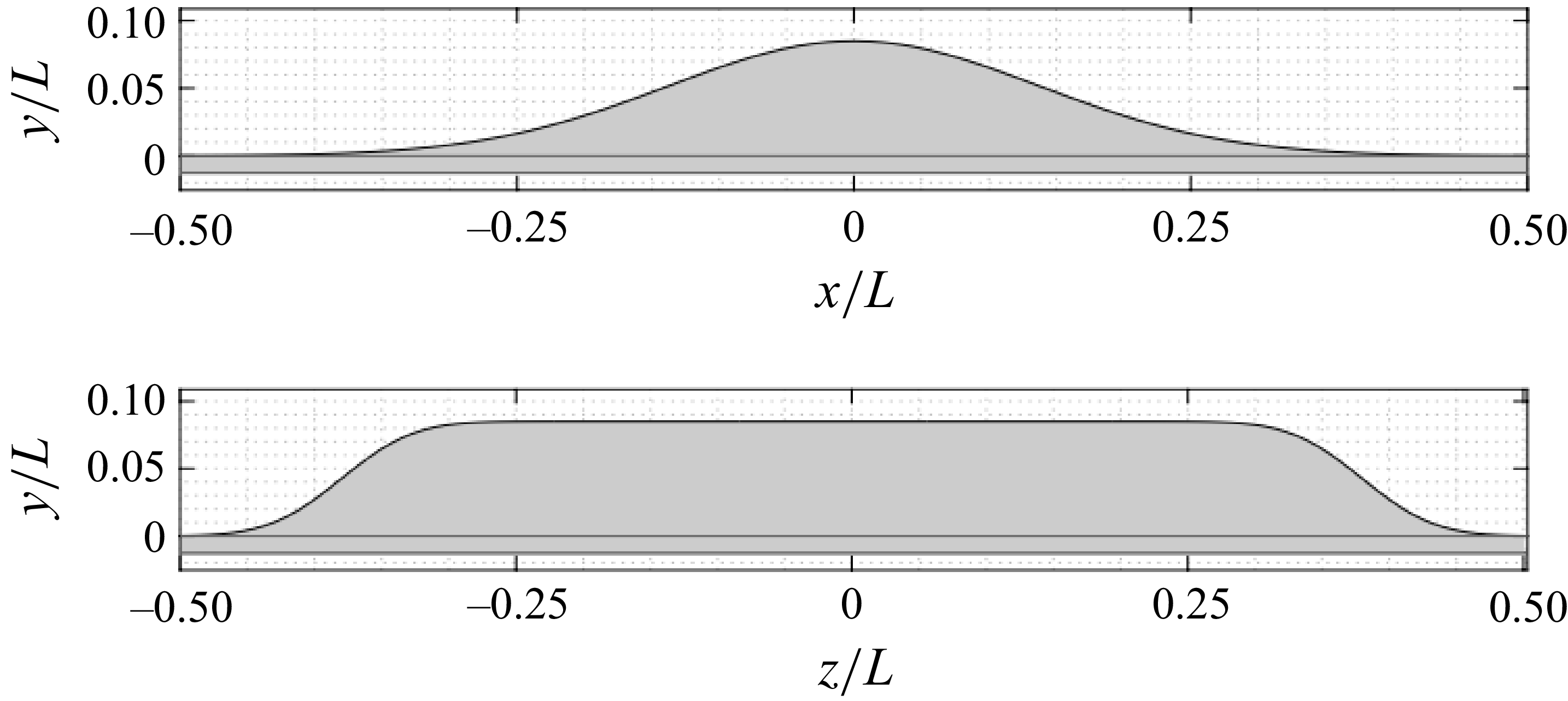


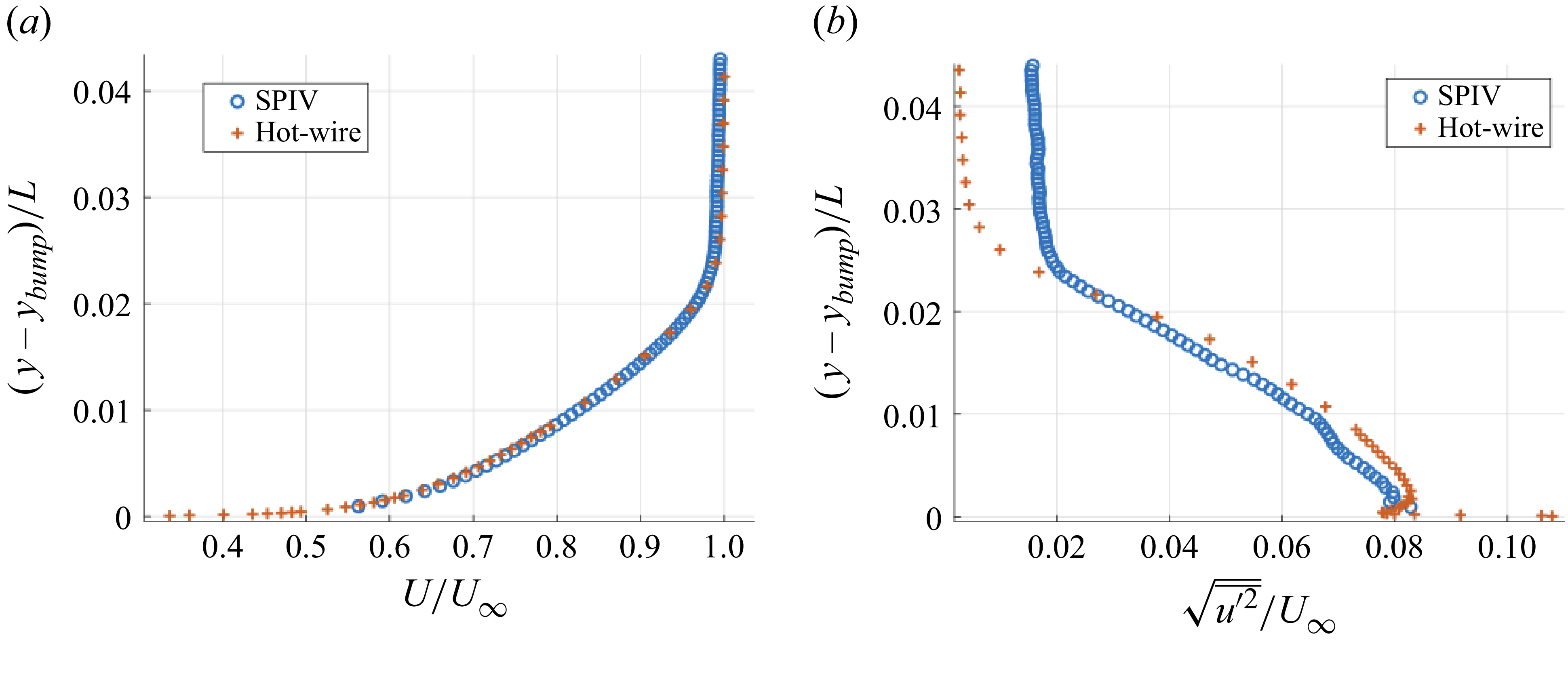


 Open access