





1. Introduction
Shock wave–turbulent boundary interactions (STBLIs) are prevalent in high-speed flows, such as those over transonic wings, in supersonic inlets and in over-expanded nozzles. A well-documented phenomenon in such flows is the low-frequency intermittent shock motion, often referred to as the breathing motion of turbulent separation bubbles (Souverein et al. Reference Souverein, Dupont, Debieve, Dussauge, Van, Bas and Scarano2010; Clemens & Narayanaswamy Reference Clemens and Narayanaswamy2014). These motions can couple with adjacent structures and generate unsteady aerodynamic loads, posing significant risks to the structural integrity of an airframe (Dolling Reference Dolling2001). This concern has motivated growing research interest in flow-control strategies aimed at mitigating the hazards associated with STBLIs.
Babinsky & Ogawa (Reference Babinsky and Ogawa2008) classified the control strategies into two main categories: boundary-layer control and shock control. Boundary-layer control aims to delay separation by modifying the upstream boundary layer, whereas shock control focuses on altering the shock structure itself. Vortex generators are widely used for boundary-layer control, producing trailing vortices that enhance momentum exchange to delay flow separation (Anderson, Tinapple & Surber Reference Anderson, Tinapple and Surber2006; Ghosh, Choi & Edwards Reference Ghosh, Choi and Edwards2008; Sun et al. Reference Sun, Guo, Li and Liu2019). Despite their ability to introduce strong three-dimensional (3-D) effects and alter the upstream boundary layer, they may not effectively suppress the inherent low-frequency unsteadiness of STBLIs. In fact, Della Posta et al. (Reference Della Posta, Martelli, Salvadore and Bernardini2024) reported that upstream vortex generators even enhanced this unsteadiness. Shock-control bumps, on the other hand, are commonly applied to transonic wings, as comprehensively reviewed by Bruce & Colliss (Reference Bruce and Colliss2015), with research emphasis placed on drag reduction and shock buffet delay. In shock impingement interactions, bumps are often employed to suppress flow separation (Nastro et al. Reference Nastro, Robinet, Loiseau, Passaggia and Mazellier2023; Ribeiro & Taira Reference Ribeiro and Taira2024). More recently, Ceci (Reference Ceci2025) shifted the focus towards attenuating the two-dimensional (2-D) low-frequency unsteadiness of the turbulent separation bubble. Through direct numerical simulations, they demonstrated that a bump shaped as the dividing streamline topology of the uncontrolled interaction can effectively eliminate flow separation and suppress low-frequency breathing motion, if appropriately positioned.
Despite these advances, most control strategies rely on trial-and-error and often introduce extra drag due to significant geometric change. This limitation stems from the incomplete physical understanding of the breathing motion, which, as noted by Clemens & Narayanaswamy (Reference Clemens and Narayanaswamy2014), is governed by coupled upstream and downstream mechanisms. Recently, a promising explanation has been proposed through stability analysis: the unsteadiness is intrinsic, governed by a 2-D global mode that is excited by external disturbances (Touber & Sandham Reference Touber and Sandham2009; Nichols et al. Reference Nichols, Larsson, Bernardini and Pirozzoli2017; Hao Reference Hao2023). This insight enables a more targeted control methodology, referred to as stability-based control, focusing on the suppression of the global mode itself. In this context, stability-based control has gained traction recently (Marquet, Sipp & Jacquin Reference Marquet, Sipp and Jacquin2008; Martinez-Cava et al. Reference Martinez-Cava, Chávez-Modena, Valero, de Vicente and Ferrer2020; Nastro et al. Reference Nastro, Robinet, Loiseau, Passaggia and Mazellier2023; Ribeiro & Taira Reference Ribeiro and Taira2024; Jung, Bhagwat & Towne Reference Jung, Bhagwat and Towne2025), owing to its physics-informed foundation, computational efficiency and straightforward implementation. A representative example is the work of Martinez-Cava et al. (Reference Martinez-Cava, Chávez-Modena, Valero, de Vicente and Ferrer2020), who proposed a micro-bump for the control of shock buffet using stability-based control. Transonic buffet is a self-sustained oscillation governed by an unsteady, globally unstable mode. Motivated by this approach, the present study aims to employ a similar stability-based control strategy to suppress the low-frequency breathing motion.
In this study, using large-eddy simulation (LES) and global stability analysis (GSA), we identify the sensitive region of the leading 2-D global mode, design and position a micro-bump accordingly and effectively suppress the low-frequency breathing motion in a supersonic compression ramp flow.
2. Numerical strategies
2.1. Geometry and free-stream parameters
A $ 25^{\circ }$
compression ramp is considered. A Cartesian coordinate system is adopted with its origin fixed at the corner. The streamwise, vertical and spanwise directions are denoted by
$ 25^{\circ }$
compression ramp is considered. A Cartesian coordinate system is adopted with its origin fixed at the corner. The streamwise, vertical and spanwise directions are denoted by $x$
,
$x$
, $y$
and
$y$
and $z$
, respectively, with the corresponding velocity components given by
$z$
, respectively, with the corresponding velocity components given by $u$
,
$u$
, $v$
and
$v$
and $w$
. The free-stream parameters are as follows: density
$w$
. The free-stream parameters are as follows: density $ \rho _{\infty }=0.314$
kg m−
$ \rho _{\infty }=0.314$
kg m− $ ^{3}$
, Mach number
$ ^{3}$
, Mach number $ M_{\infty }=2.95$
, temperature
$ M_{\infty }=2.95$
, temperature $ T_{\infty }= 108$
K and Reynolds number
$ T_{\infty }= 108$
K and Reynolds number $ \textit{Re}_{\delta }=63\,500$
based on the boundary-layer thickness
$ \textit{Re}_{\delta }=63\,500$
based on the boundary-layer thickness $\delta$
at the reference station
$\delta$
at the reference station $x=-15.4\delta$
. The flow is modelled as a perfect gas with a specific heat ratio of 1.4 and a Prandtl number of 0.72. The molecular viscosity
$x=-15.4\delta$
. The flow is modelled as a perfect gas with a specific heat ratio of 1.4 and a Prandtl number of 0.72. The molecular viscosity $\mu$
is calculated using Sutherland’s law.
$\mu$
is calculated using Sutherland’s law.
2.2. Computational set-up
Implicit LES are conducted using an in-house solver named PHAROS (Hao & Wen Reference Hao and Wen2020). The inviscid fluxes are computed using a sixth-order skew-symmetric central difference scheme (Pirozzoli Reference Pirozzoli2010) in smooth-flow regions. In regions containing discontinuities, the scheme is switched to the AUSM $^{+}$
-up scheme (Liou Reference Liou2006) with a fifth-order weighted essentially non-oscillatory reconstruction (Jiang & Shu Reference Jiang and Shu1996). The switching is controlled by a modified Jameson sensor (Jameson, Schmidt & Turkel Reference Jameson, Schmidt and Turkel1981), with a threshold of 0.1. The viscous terms are discretised using a second-order central difference scheme, and time integration is carried out with a third-order Runge–Kutta method.
$^{+}$
-up scheme (Liou Reference Liou2006) with a fifth-order weighted essentially non-oscillatory reconstruction (Jiang & Shu Reference Jiang and Shu1996). The switching is controlled by a modified Jameson sensor (Jameson, Schmidt & Turkel Reference Jameson, Schmidt and Turkel1981), with a threshold of 0.1. The viscous terms are discretised using a second-order central difference scheme, and time integration is carried out with a third-order Runge–Kutta method.
Turbulent inflow is generated using the modified digital filter technique (Touber & Sandham Reference Touber and Sandham2009). A non-reflective boundary condition (Mani Reference Mani2012) is applied at the upper domain boundary, while the outflow boundary uses a simple extrapolation, which is located far downstream of the interaction region with a stretched grid applied as a sponge zone. The streamwise distance between the outflow boundary and the corner is approximately 20 $\delta$
, while the sponge zone lasts for 6
$\delta$
, while the sponge zone lasts for 6 $\delta$
. The wall is treated as isothermal with a fixed temperature of
$\delta$
. The wall is treated as isothermal with a fixed temperature of $T_w = 275.4$
K. Periodic boundary conditions are imposed in the spanwise direction, which has a width of
$T_w = 275.4$
K. Periodic boundary conditions are imposed in the spanwise direction, which has a width of $4\delta$
. Although this domain width is insufficient to resolve the large-scale 3-D spanwise undulations reported in recent numerical and experimental studies (Ceci et al. Reference Ceci, Palumbo, Larsson and Pirozzoli2023; Liu et al. Reference Liu, Chen, Zhang, Tan, Liu and Peng2024), Zhang et al. (Reference Zhang, Li and Hao2025b
) showed that the quasi-2-D breathing motion is the dominant factor in wall-pressure response. This conclusion is supported by several numerical investigations demonstrating that experimental wall-pressure fluctuations can be accurately reproduced with comparably narrow computational domains (Pasquariello, Hickel & Adams Reference Pasquariello, Hickel and Adams2017; Fang et al. Reference Fang, Zheltovodov, Yao, Moulinec and Emerson2020; Bernardini et al. Reference Bernardini, Della Posta, Salvadore and Martelli2023). A detailed discussion of the effects of spanwise widths is provided in Appendix A. At the reference station, the grid resolutions in wall units are approximately
$4\delta$
. Although this domain width is insufficient to resolve the large-scale 3-D spanwise undulations reported in recent numerical and experimental studies (Ceci et al. Reference Ceci, Palumbo, Larsson and Pirozzoli2023; Liu et al. Reference Liu, Chen, Zhang, Tan, Liu and Peng2024), Zhang et al. (Reference Zhang, Li and Hao2025b
) showed that the quasi-2-D breathing motion is the dominant factor in wall-pressure response. This conclusion is supported by several numerical investigations demonstrating that experimental wall-pressure fluctuations can be accurately reproduced with comparably narrow computational domains (Pasquariello, Hickel & Adams Reference Pasquariello, Hickel and Adams2017; Fang et al. Reference Fang, Zheltovodov, Yao, Moulinec and Emerson2020; Bernardini et al. Reference Bernardini, Della Posta, Salvadore and Martelli2023). A detailed discussion of the effects of spanwise widths is provided in Appendix A. At the reference station, the grid resolutions in wall units are approximately $\Delta x^{+} \approx 19$
,
$\Delta x^{+} \approx 19$
, $\Delta y_{w}^{+} \approx 1.0$
and
$\Delta y_{w}^{+} \approx 1.0$
and $\Delta z^{+} \approx 10$
. For the solver validation, the reader is referred to Zhang et al. (Reference Zhang, Li and Hao2025b
).
$\Delta z^{+} \approx 10$
. For the solver validation, the reader is referred to Zhang et al. (Reference Zhang, Li and Hao2025b
).
2.3. Global stability analysis
The linearised Navier–Stokes equation in the operator form is written as
 \begin{align} \frac {\partial \boldsymbol{{U^{\prime }}} }{\partial t}=\boldsymbol{\mathcal{A}}\boldsymbol{{U^{\prime }}}, \end{align}
where $\boldsymbol{{U^{\prime }}}$
is a small-amplitude 3-D perturbation vector and
$\boldsymbol{{U^{\prime }}}$
is a small-amplitude 3-D perturbation vector and $\boldsymbol{\mathcal{A}}$
is the linearised Navier–Stokes operator. The perturbation term is assumed in the following modal norm:
$\boldsymbol{\mathcal{A}}$
is the linearised Navier–Stokes operator. The perturbation term is assumed in the following modal norm:
 \begin{align} \boldsymbol{{U^{\prime }}}(x,y,z,t) = \boldsymbol{\hat {U}}(x,y)\mathrm{exp}\left [ i\beta z-i({\omega }_{r}+i{\omega }_{i})t\right ], \end{align}
where $\boldsymbol{\hat {U}}$
is the 2-D function,
$\boldsymbol{\hat {U}}$
is the 2-D function, $\beta$
represents the spanwise wavenumber,
$\beta$
represents the spanwise wavenumber, ${\omega }_{r}$
denotes the angular frequency and
${\omega }_{r}$
denotes the angular frequency and ${\omega }_{i}$
indicates the growth rate. Here
${\omega }_{i}$
indicates the growth rate. Here ${\omega }_{i}\gt 0$
means a flow is globally unstable (and vice versa). Substituting (2.2) into (2.1) leads to an eigenvalue problem, which can be solved using an in-house GSA solver as described in Hao (Reference Hao2023). Note that an effective viscosity
${\omega }_{i}\gt 0$
means a flow is globally unstable (and vice versa). Substituting (2.2) into (2.1) leads to an eigenvalue problem, which can be solved using an in-house GSA solver as described in Hao (Reference Hao2023). Note that an effective viscosity $\mu _{eff}=\mu _{t}+\mu$
is adopted, where
$\mu _{eff}=\mu _{t}+\mu$
is adopted, where $\mu _{t}$
is the eddy viscosity obtained using a least-squares fit method (Lilly Reference Lilly1992). The formulation of
$\mu _{t}$
is the eddy viscosity obtained using a least-squares fit method (Lilly Reference Lilly1992). The formulation of $\mu _{t}$
is detailed in Appendix B. A sponge layer is placed near the left boundary (Mani Reference Mani2012) to avoid any introduction of disturbances, while the remaining boundaries are treated consistently with the LES.
$\mu _{t}$
is detailed in Appendix B. A sponge layer is placed near the left boundary (Mani Reference Mani2012) to avoid any introduction of disturbances, while the remaining boundaries are treated consistently with the LES.
Real parts of ( $ a$
) the 2-D global mode and (
$ a$
) the 2-D global mode and ( $ b$
) the leading 2-D SPOD mode at
$ b$
) the leading 2-D SPOD mode at $ St=0.026$
. (
$ St=0.026$
. ( $c$
) Normalised energy distribution of SPOD modes; the red dashed line marks the frequency
$c$
) Normalised energy distribution of SPOD modes; the red dashed line marks the frequency $ \textit{St}=0.026$
. (
$ \textit{St}=0.026$
. ( $d$
) Wall-normal integrated Chu energy density for the 2-D global mode and and SPOD modes, normalised by their respective maximum values. The SPOD details: Welch method with a Hamming window, eight segments, 75
$d$
) Wall-normal integrated Chu energy density for the 2-D global mode and and SPOD modes, normalised by their respective maximum values. The SPOD details: Welch method with a Hamming window, eight segments, 75 $\,\%$
overlap, segment length
$\,\%$
overlap, segment length $194L_{\textit{sep}}/u_{\infty }$
.
$194L_{\textit{sep}}/u_{\infty }$
.

3. Results
3.1. The low-frequency unsteadiness
Hao (Reference Hao2023) demonstrated that 2-D shock motion is primarily driven by a 2-D global mode (referred to as the shock mode), characterised by $\beta =0$
and
$\beta =0$
and ${\omega }_{r} =0$
, through a modal resonance mechanism. The interpretation, however, relies on Reynolds-averaged Navier–Stokes (RANS) simulations and RANS-based GSA. As a result, direct evidence for the physical existence of the mode was not established. In the present work, this issue is revisited by comparing 2-D coherent structures extracted from LES with the 2-D global mode obtained from LES-based GSA, thereby providing higher-fidelity support for the underlying mechanism. Spectral proper orthogonal decomposition (SPOD) analysis is performed to extract coherent structures from the unsteady spanwise-averaged data. The input data consist of the spanwise-averaged state vector
${\omega }_{r} =0$
, through a modal resonance mechanism. The interpretation, however, relies on Reynolds-averaged Navier–Stokes (RANS) simulations and RANS-based GSA. As a result, direct evidence for the physical existence of the mode was not established. In the present work, this issue is revisited by comparing 2-D coherent structures extracted from LES with the 2-D global mode obtained from LES-based GSA, thereby providing higher-fidelity support for the underlying mechanism. Spectral proper orthogonal decomposition (SPOD) analysis is performed to extract coherent structures from the unsteady spanwise-averaged data. The input data consist of the spanwise-averaged state vector $ {q}^{\prime }= [ \rho ^{\prime },u^{\prime },v^{\prime },w^{\prime },T^{\prime } ]$
. Welch’s method is used with a Hamming window to minimise spectral leakage, segmenting the dataset into eight blocks with 75
$ {q}^{\prime }= [ \rho ^{\prime },u^{\prime },v^{\prime },w^{\prime },T^{\prime } ]$
. Welch’s method is used with a Hamming window to minimise spectral leakage, segmenting the dataset into eight blocks with 75 $ \,\%$
overlap. The Chu energy norm (Chu Reference Chu1965) is used as the inner product. The use of spanwise-averaged SPOD is appropriate owing to the quasi-2-D character of the shock motion in ramp flows (Clemens & Narayanaswamy Reference Clemens and Narayanaswamy2014). Figure 1(
$ \,\%$
overlap. The Chu energy norm (Chu Reference Chu1965) is used as the inner product. The use of spanwise-averaged SPOD is appropriate owing to the quasi-2-D character of the shock motion in ramp flows (Clemens & Narayanaswamy Reference Clemens and Narayanaswamy2014). Figure 1( $a{,}b$
) compares the 2-D shock mode and the leading 2-D SPOD mode at the normalised frequency
$a{,}b$
) compares the 2-D shock mode and the leading 2-D SPOD mode at the normalised frequency $ St=fL_{\textit{sep}}/u_{\infty }=0.026$
, where
$ St=fL_{\textit{sep}}/u_{\infty }=0.026$
, where $L_{\textit{sep}}$
is the separation length and
$L_{\textit{sep}}$
is the separation length and $u_{\infty }$
is the free-stream velocity. Note that
$u_{\infty }$
is the free-stream velocity. Note that $L_{\textit{sep}}$
from the uncontrolled case is used in the definition of
$L_{\textit{sep}}$
from the uncontrolled case is used in the definition of $ \textit{St}$
throughout this study to ensure consistent comparison. This frequency corresponds the energy peak of the SPOD modes in the low-frequency regime, as shown in figure 1(
$ \textit{St}$
throughout this study to ensure consistent comparison. This frequency corresponds the energy peak of the SPOD modes in the low-frequency regime, as shown in figure 1( $c$
), and aligns well with the characteristic frequency of the shock motion presented later in figure 2(
$c$
), and aligns well with the characteristic frequency of the shock motion presented later in figure 2( $ c$
). The shock mode maintains high values of
$ c$
). The shock mode maintains high values of $ u^{\prime }$
near the shock foot and along the separation shock. Notably, the SPOD mode closely resembles the shock mode, with elevated
$ u^{\prime }$
near the shock foot and along the separation shock. Notably, the SPOD mode closely resembles the shock mode, with elevated $ u^{\prime }$
values similarly concentrated around the shock foot and along the shock. Convergence of the SPOD modes is discussed in Appendix C.
$ u^{\prime }$
values similarly concentrated around the shock foot and along the shock. Convergence of the SPOD modes is discussed in Appendix C.
A quantitative comparison between the two modes can be conducted using two methods. First, the integrated Chu energy density distributions along the streamwise direction are compared, as shown in figure 1( $ d$
). Both distributions are normalised by their respective peak values located just downstream of the mean separation point
$ d$
). Both distributions are normalised by their respective peak values located just downstream of the mean separation point $x_{\textit{sep}}$
. Slightly upstream of
$x_{\textit{sep}}$
. Slightly upstream of $x_{\textit{sep}}$
, both profiles increase rapidly towards their peaks. Their growth rates and positions closely match. Downstream of these peaks, both distributions exhibit a gradual decline, followed by an increase beyond the corner. Despite minor differences in the decay rates, the overall trends remain highly similar. This consistent behaviour provides compelling evidence that the two modes share fundamental similarities. The second perspective is to make a projection between the two modes, given by
$x_{\textit{sep}}$
, both profiles increase rapidly towards their peaks. Their growth rates and positions closely match. Downstream of these peaks, both distributions exhibit a gradual decline, followed by an increase beyond the corner. Despite minor differences in the decay rates, the overall trends remain highly similar. This consistent behaviour provides compelling evidence that the two modes share fundamental similarities. The second perspective is to make a projection between the two modes, given by
 \begin{align} \gamma =\frac {\big | {\parallel \boldsymbol{{\hat {\varPsi }}_{\textit{SPOD}}}(x,y), \boldsymbol{{\hat {U}}_{\textit{GSA}}}(x,y)\parallel }_{E} \big |}{ {\parallel \boldsymbol{{\hat {\varPsi }}_{\textit{SPOD}}}(x,y) \parallel }_{E} \times {\parallel \boldsymbol{{\hat {U}}_{\textit{GSA}}}(x,y)\parallel }_{E} }, \end{align}
where $ \boldsymbol{{\hat {\varPsi }}_{\textit{SPOD}}}(x,y)$
represents the 2-D leading SPOD mode at
$ \boldsymbol{{\hat {\varPsi }}_{\textit{SPOD}}}(x,y)$
represents the 2-D leading SPOD mode at $ \textit{St}=0.026$
, while
$ \textit{St}=0.026$
, while $ \boldsymbol{{\hat {U}}_{\textit{GSA}}}(x,y)$
denotes the shock mode. The notation
$ \boldsymbol{{\hat {U}}_{\textit{GSA}}}(x,y)$
denotes the shock mode. The notation $ \left \| \boldsymbol{\cdot }\right \|_{E}$
means the Chu norm (Chu Reference Chu1965). A value of
$ \left \| \boldsymbol{\cdot }\right \|_{E}$
means the Chu norm (Chu Reference Chu1965). A value of $ \gamma =1$
represents a perfect match of the two modes. The projection coefficient between the two modes shown in figure 1(
$ \gamma =1$
represents a perfect match of the two modes. The projection coefficient between the two modes shown in figure 1( $ a{,}b$
) is 0.93, indicating a strong correlation between them. This further supports the conclusion that the low-frequency unsteadiness of the turbulent separation bubble is predominantly driven by the shock mode. Moreover, the low-frequency shock motion can be effectively reconstructed by superimposing the leading SPOD mode at
$ a{,}b$
) is 0.93, indicating a strong correlation between them. This further supports the conclusion that the low-frequency unsteadiness of the turbulent separation bubble is predominantly driven by the shock mode. Moreover, the low-frequency shock motion can be effectively reconstructed by superimposing the leading SPOD mode at $ \textit{St}=0.026$
onto the mean flow (see supplementary movie available at https://doi.org/10.1017/jfm.2026.11679).
$ \textit{St}=0.026$
onto the mean flow (see supplementary movie available at https://doi.org/10.1017/jfm.2026.11679).
3.2. Controlled breathing motion with a micro-bump
Having established the central role of the 2-D global mode in driving the low-frequency unsteadiness, we now turn to its targeted suppression by exploiting its sensitivity distribution. Following Paladini et al. (Reference Paladini, Marquet, Sipp, Robinet and Dandois2019), the core of the 2-D instability can be quantified by the complex density $ d= \tilde {U} ^{\dagger } \hat {U}$
, where
$ d= \tilde {U} ^{\dagger } \hat {U}$
, where $ \tilde {U}$
is the 2-D adjoint mode and the superscript
$ \tilde {U}$
is the 2-D adjoint mode and the superscript $ \dagger$
refers to the transconjugate. The adjoint mode is computed by solving the adjoint eigenvalue problem. The real part of
$ \dagger$
refers to the transconjugate. The adjoint mode is computed by solving the adjoint eigenvalue problem. The real part of $ d$
represents the local contribution to the growth rate of the zero-frequency shock mode. Note that the integration of
$ d$
represents the local contribution to the growth rate of the zero-frequency shock mode. Note that the integration of $ d$
over the computational domain equals 1. Figure 2(
$ d$
over the computational domain equals 1. Figure 2( $ a$
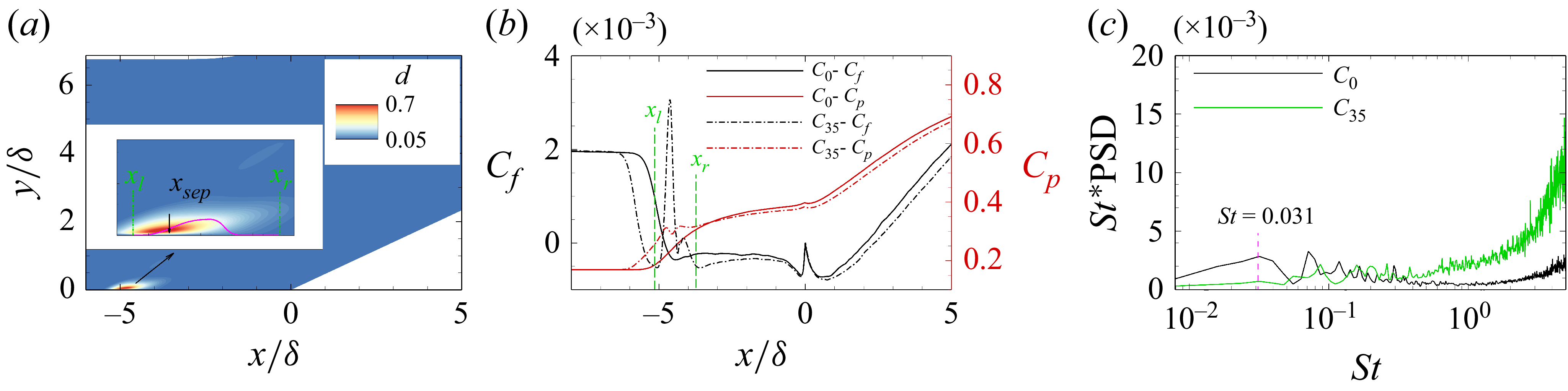
) shows the growth rate density map for the shock mode. The highest density values are concentrated near the shock foot, consistent with the mode structure shown in figure 1(
$ a$
) shows the growth rate density map for the shock mode. The highest density values are concentrated near the shock foot, consistent with the mode structure shown in figure 1( $a$
). In contrast, the density remains nearly zero elsewhere, including across the separation shock. This localised distribution indicates that the shock-foot region dominates the sensitivity to global instabilities, a finding consistent with Paladini et al. (Reference Paladini, Marquet, Sipp, Robinet and Dandois2019) in the research of transonic shock buffet, which is governed by a globally unstable, oscillatory mode.
$a$
). In contrast, the density remains nearly zero elsewhere, including across the separation shock. This localised distribution indicates that the shock-foot region dominates the sensitivity to global instabilities, a finding consistent with Paladini et al. (Reference Paladini, Marquet, Sipp, Robinet and Dandois2019) in the research of transonic shock buffet, which is governed by a globally unstable, oscillatory mode.
Parameters in (3.2): $h$
, bump height;
$h$
, bump height; $x_{l}$
and
$x_{l}$
and $x_{r}$
, left and right boundaries;
$x_{r}$
, left and right boundaries; $x_{p}$
, bump peak location;
$x_{p}$
, bump peak location; $A$
,
$A$
, $B$
,
$B$
, $C$
and
$C$
and $D$
, shape-control constants.
$D$
, shape-control constants.

( $a$
) Real part of the shock mode’s growth rate density map, with the bump edges
$a$
) Real part of the shock mode’s growth rate density map, with the bump edges $x_{l}$
and
$x_{l}$
and $x_{r}$
marked by green lines. (
$x_{r}$
marked by green lines. ( $b$
) Comparison of skin-friction (
$b$
) Comparison of skin-friction ( $C_f$
) and pressure (
$C_f$
) and pressure ( $C_p$
) coefficients. (
$C_p$
) coefficients. ( $c$
) Pre-multiplied wall-pressure spectra at station
$c$
) Pre-multiplied wall-pressure spectra at station $x_{\textit{sep}}$
(case
$x_{\textit{sep}}$
(case $C_{0}$
) and station
$C_{0}$
) and station $x_{p}$
(case
$x_{p}$
(case $C_{35}$
).
$C_{35}$
).

To mitigate the instability contribution from the shock-foot region, we introduce a local surface modification. Inspired by Martinez-Cava et al. (Reference Martinez-Cava, Chávez-Modena, Valero, de Vicente and Ferrer2020), who showed that the optimal surface deformation for weakening shock-buffet instability resembles a shock-control bump, we adopt a similar control bump around the shock-foot region, as highlighted by the purple line in the inset of figure 2( $a$
). This small-scale bump is designed to control the shock mode and suppress the low-frequency shock motion. The geometric configuration of the bump is defined by the following shape function:
$a$
). This small-scale bump is designed to control the shock mode and suppress the low-frequency shock motion. The geometric configuration of the bump is defined by the following shape function:
 \begin{align} y=\begin{cases}h_{1} \times (1-\mathrm{exp}(-(x-x_{p}+A )^{B})) & \text{ if } x_{l}\le x\lt x_{p}, \\h_{2} \times (1-\mathrm{tanh}(C\times (x-x_{p}+D))) & \text{ if } x_{p}\le x\le x_{r}. \end{cases} \end{align}
Here, $ h_{1} =h/(1-\mathrm{exp}(-A^{B} ))$
and
$ h_{1} =h/(1-\mathrm{exp}(-A^{B} ))$
and $ h_{2} =h/(1-\mathrm{tanh}(C\times D))$
are scaling factors, where
$ h_{2} =h/(1-\mathrm{tanh}(C\times D))$
are scaling factors, where $h$
is the bump height. The streamwise extent and positioning of the bump are defined by
$h$
is the bump height. The streamwise extent and positioning of the bump are defined by $x_{l}$
and
$x_{l}$
and $x_{r}$
marking the left and right boundaries, respectively, and
$x_{r}$
marking the left and right boundaries, respectively, and $x_{p}$
indicating the peak location. Constants
$x_{p}$
indicating the peak location. Constants $ A$
,
$ A$
, $ B$
,
$ B$
, $ C$
and
$ C$
and $D$
govern the bump profile. Values of these parameters are listed in table 1. The bump is designed primarily to envelop the high-sensitivity region and centre around the separation point
$D$
govern the bump profile. Values of these parameters are listed in table 1. The bump is designed primarily to envelop the high-sensitivity region and centre around the separation point $x_{\textit{sep}}$
, featuring a gradual ascent followed by a steep descent. The smooth forward rise prevents additional separation, while the steeper rear section serves to modify the separation bubble. The bump size is relatively small, with a height 15
$x_{\textit{sep}}$
, featuring a gradual ascent followed by a steep descent. The smooth forward rise prevents additional separation, while the steeper rear section serves to modify the separation bubble. The bump size is relatively small, with a height 15 $\,\%$
of the boundary-layer thickness and a streamwise length 20
$\,\%$
of the boundary-layer thickness and a streamwise length 20 $\,\%$
of the separation length. Hereafter, the uncontrolled case is denoted as
$\,\%$
of the separation length. Hereafter, the uncontrolled case is denoted as $C_{0}$
and the controlled case as
$C_{0}$
and the controlled case as $C_{35}$
, where the subscript denotes the bump height.
$C_{35}$
, where the subscript denotes the bump height.
The flow response to the introduction of the micro-bump is examined next. Figure 2( $b$
) compares the skin-friction coefficient
$b$
) compares the skin-friction coefficient $ C_{f}$
and pressure coefficient
$ C_{f}$
and pressure coefficient $ C_{p}$
. For
$ C_{p}$
. For $C_{35}$
, the bump induces a mild adverse pressure gradient upstream, leading to a minor localised separation ahead of the bump. Near the bump peak, the
$C_{35}$
, the bump induces a mild adverse pressure gradient upstream, leading to a minor localised separation ahead of the bump. Near the bump peak, the $ C_{f}$
distribution shows a pronounced increase, while that of
$ C_{f}$
distribution shows a pronounced increase, while that of $ C_{p}$
exhibits slight fluctuations followed by a recovery. Away from the bump region, both
$ C_{p}$
exhibits slight fluctuations followed by a recovery. Away from the bump region, both $ C_{f}$
and
$ C_{f}$
and $ C_{p}$
distributions closely match those of
$ C_{p}$
distributions closely match those of $ C_{0}$
, confirming that the influence of the bump remains highly localised. Over the range
$ C_{0}$
, confirming that the influence of the bump remains highly localised. Over the range $(-10\delta , 8\delta )$
, the integrated skin-friction drag of the controlled case
$(-10\delta , 8\delta )$
, the integrated skin-friction drag of the controlled case $C_{35}$
is reduced by
$C_{35}$
is reduced by $14\,\%$
compared with that of case
$14\,\%$
compared with that of case $C_{0}$
, while the pressure drag decreases by 0.8
$C_{0}$
, while the pressure drag decreases by 0.8 $\,\%$
.
$\,\%$
.
The primary differences emerge in the power spectral density (PSD) spectra near the bump region, as illustrated in figure 2( $c$
). Here, we choose the station
$c$
). Here, we choose the station $ x_{\textit{sep}}$
from case
$ x_{\textit{sep}}$
from case $C_{0}$
and
$C_{0}$
and $x_{p}$
from case
$x_{p}$
from case $C_{35}$
for comparison, where the low-frequency motion is evident. In the low-frequency regime (
$C_{35}$
for comparison, where the low-frequency motion is evident. In the low-frequency regime ( $ \textit{St}\lt 0.05$
), a predominant peak is observed at
$ \textit{St}\lt 0.05$
), a predominant peak is observed at $ \textit{St}=0.031$
, which corresponds to the low-frequency breathing motion. However, this peak diminishes in the
$ \textit{St}=0.031$
, which corresponds to the low-frequency breathing motion. However, this peak diminishes in the $C_{35}$
case. With increasing
$C_{35}$
case. With increasing $ \textit{St}$
, high-frequency energy is gradually amplified. A similar trend was also reported by Ceci (Reference Ceci2025), where a large shock-control bump was implemented.
$ \textit{St}$
, high-frequency energy is gradually amplified. A similar trend was also reported by Ceci (Reference Ceci2025), where a large shock-control bump was implemented.
Instantaneous vortices from ( $ a$
)
$ a$
) $C_{0}$
and (
$C_{0}$
and ( $ b$
)
$ b$
) $C_{35}$
, extracted using the
$C_{35}$
, extracted using the $ Q$
-criterion, 5
$ Q$
-criterion, 5 $ \,\%$
of the maximum of
$ \,\%$
of the maximum of $C_{0}$
, coloured by the Favre-fluctuating velocity
$C_{0}$
, coloured by the Favre-fluctuating velocity $ u^{\prime\prime}/u_{\infty }$
. Transparent iso-surfaces of density-gradient magnitude are used to highlight the shock position.
$ u^{\prime\prime}/u_{\infty }$
. Transparent iso-surfaces of density-gradient magnitude are used to highlight the shock position.

A comparison of the instantaneous vortices, coloured by the fluctuating velocity $ u^{\prime\prime}/u_{\infty }$
, is presented in figure 3 for the two cases. Upstream of the separation shock, both cases exhibit negligible vortex activity. In the uncontrolled case
$ u^{\prime\prime}/u_{\infty }$
, is presented in figure 3 for the two cases. Upstream of the separation shock, both cases exhibit negligible vortex activity. In the uncontrolled case $C_{0}$
, vortices primarily originate near the shock foot and subsequently propagate downstream. While for the controlled
$C_{0}$
, vortices primarily originate near the shock foot and subsequently propagate downstream. While for the controlled $C_{35}$
case, the micro-bump acts as an effective vortex generator, shedding numerous small-scale vortices in its immediate vicinity. Downstream of the bump, the large-scale vortices are significantly reduced compared with case
$C_{35}$
case, the micro-bump acts as an effective vortex generator, shedding numerous small-scale vortices in its immediate vicinity. Downstream of the bump, the large-scale vortices are significantly reduced compared with case $C_{0}$
. This distinct alteration in the flow pattern demonstrates that the bump fundamentally modifies the vortex dynamics of the interaction.
$C_{0}$
. This distinct alteration in the flow pattern demonstrates that the bump fundamentally modifies the vortex dynamics of the interaction.
( $a$
) Comparison of the eigenvalues for the 2-D modes from cases
$a$
) Comparison of the eigenvalues for the 2-D modes from cases $C_{0}$
and
$C_{0}$
and $C_{35}$
. Real parts of (
$C_{35}$
. Real parts of ( $ b$
) the 2-D mode and (
$ b$
) the 2-D mode and ( $ c$
) the leading SPOD mode at
$ c$
) the leading SPOD mode at $ \textit{St}=0.03$
for case
$ \textit{St}=0.03$
for case $C_{35}$
. (
$C_{35}$
. ( $d$
) Low-pass-filtered planar TKE distributions (
$d$
) Low-pass-filtered planar TKE distributions ( $ \textit{St}_{cut}=0.1$
), normalised by the square of the friction velocity
$ \textit{St}_{cut}=0.1$
), normalised by the square of the friction velocity $u_{\tau }^{2}$
at the reference station. Streamwise distributions of (
$u_{\tau }^{2}$
at the reference station. Streamwise distributions of ( $e$
) the wall-normal integrated TKE (
$e$
) the wall-normal integrated TKE ( $ \textit{St}_{cut}=0.1$
) and (
$ \textit{St}_{cut}=0.1$
) and ( $f$
) the normalised wall-pressure root mean square (
$f$
) the normalised wall-pressure root mean square ( $ \textit{St}_{cut}=0.1$
) for both cases. Black lines in (
$ \textit{St}_{cut}=0.1$
) for both cases. Black lines in ( $d$
) indicate dividing streamlines. Green dash-dot and solid lines in (
$d$
) indicate dividing streamlines. Green dash-dot and solid lines in ( $c$
,
$c$
, $d$
) mark the edges and peak positions of the bump, respectively. Both TKE and
$d$
) mark the edges and peak positions of the bump, respectively. Both TKE and $p^{\prime}_{\textit{rms}} /\bar {p}_{w}$
in (
$p^{\prime}_{\textit{rms}} /\bar {p}_{w}$
in ( $e$
,
$e$
, $f$
) are normalised by the peak values of the
$f$
) are normalised by the peak values of the $C_{0}$
case.
$C_{0}$
case.

The GSA reveals a fundamental change in the 2-D dynamics. As shown in figure 4( $a$
), the most unstable 2-D global mode in case
$a$
), the most unstable 2-D global mode in case $C_{0}$
is strongly damped in case
$C_{0}$
is strongly damped in case $C_{35}$
, transitioning to a stable mode. Its spatial structure also shifts, with high
$C_{35}$
, transitioning to a stable mode. Its spatial structure also shifts, with high $u^{\prime}$
amplitudes now concentrated along the shear layer from the bump and the separation shock, rather than at the shock foot, as shown in figure 4(
$u^{\prime}$
amplitudes now concentrated along the shear layer from the bump and the separation shock, rather than at the shock foot, as shown in figure 4( $b$
). Although stabilised, this mode is still excited by disturbances through modal resonance. The leading SPOD mode at
$b$
). Although stabilised, this mode is still excited by disturbances through modal resonance. The leading SPOD mode at $ \textit{St}=0.03$
(figure 4
$ \textit{St}=0.03$
(figure 4 $c$
) confirms this, showing strong similarity to the global mode (projection coefficient of 0.89 with the global mode). Crucially, the stable mode is associated with weak breathing motion, as evidenced by the reconstructed unsteady flow fields obtained using the specific SPOD mode (see supplementary movie). Furthermore, the long-time filtered unsteady density gradient magnitude with
$c$
) confirms this, showing strong similarity to the global mode (projection coefficient of 0.89 with the global mode). Crucially, the stable mode is associated with weak breathing motion, as evidenced by the reconstructed unsteady flow fields obtained using the specific SPOD mode (see supplementary movie). Furthermore, the long-time filtered unsteady density gradient magnitude with $ \textit{St}_{cut}=0.05$
for the two cases is also provided in the supplementary movies, which clearly show weakened shock motion. Convergence of the SPOD modes is verified in Appendix C.
$ \textit{St}_{cut}=0.05$
for the two cases is also provided in the supplementary movies, which clearly show weakened shock motion. Convergence of the SPOD modes is verified in Appendix C.
The strength of the low-frequency breathing motion is then quantified and compared for cases $ C_{0}$
and
$ C_{0}$
and $ C_{35}$
. Here, we compare their wall-normal integrated planar turbulent kinetic energy (TKE) distributions and wall-pressure fluctuations (
$ C_{35}$
. Here, we compare their wall-normal integrated planar turbulent kinetic energy (TKE) distributions and wall-pressure fluctuations ( $ p^{\prime}_{\textit{rms}}$
). Both quantities are low-pass filtered at
$ p^{\prime}_{\textit{rms}}$
). Both quantities are low-pass filtered at $ \textit{St}_{cut}=0.1$
to focus on the low-frequency dynamics. The planar TKE is defined as follows:
$ \textit{St}_{cut}=0.1$
to focus on the low-frequency dynamics. The planar TKE is defined as follows:
 \begin{align} \mathrm{Planar\;TKE}=0.5\times \big [ \big \langle u^{\prime\prime}_{\textit{span}}u^{\prime\prime}_{\textit{span}} \big \rangle +\big\langle v^{\prime\prime}_{\textit{span}}v^{\prime\prime}_{\textit{span}} \big \rangle \big], \end{align}
where the spanwise averaging (denoted by the subscript ‘ $ span$
’) and the omission of the small
$ span$
’) and the omission of the small $\langle w^{\prime\prime}_{\textit{span}}w^{\prime\prime}_{\textit{span}} \rangle$
term are deliberate choices to isolate the dominant 2-D motion from 3-D turbulent fluctuations. This operation is reasonable since the total TKE is mainly contributed by the planar part, as compared in figure 4(
$\langle w^{\prime\prime}_{\textit{span}}w^{\prime\prime}_{\textit{span}} \rangle$
term are deliberate choices to isolate the dominant 2-D motion from 3-D turbulent fluctuations. This operation is reasonable since the total TKE is mainly contributed by the planar part, as compared in figure 4( $e$
). The operator
$e$
). The operator $\left \langle \boldsymbol{\cdot }\right \rangle$
signifies the Favre average and the double prime marks the Favre fluctuating variables.
$\left \langle \boldsymbol{\cdot }\right \rangle$
signifies the Favre average and the double prime marks the Favre fluctuating variables.
In figure 4( $d$
), the filtered TKE distributions of the two cases are presented, normalised by the square of the friction velocity at the reference station and superimposed with the dividing streamlines. In the uncontrolled
$d$
), the filtered TKE distributions of the two cases are presented, normalised by the square of the friction velocity at the reference station and superimposed with the dividing streamlines. In the uncontrolled $C_{0}$
case, regions of high TKE are concentrated around the shock foot and along the separation shock, exhibiting a striking resemblance to the structure of the 2-D global mode shown in figure 1(
$C_{0}$
case, regions of high TKE are concentrated around the shock foot and along the separation shock, exhibiting a striking resemblance to the structure of the 2-D global mode shown in figure 1( $a{,} b$
). This spatial agreement strongly indicates that the low-frequency TKE is governed by this 2-D global mode. In the controlled
$a{,} b$
). This spatial agreement strongly indicates that the low-frequency TKE is governed by this 2-D global mode. In the controlled $C_{35}$
case, the TKE distribution continues to broadly follow the shape of the stabilised global mode from figure 4(
$C_{35}$
case, the TKE distribution continues to broadly follow the shape of the stabilised global mode from figure 4( $b{,} c$
), though with visibly attenuated amplitudes compared to the uncontrolled case.
$b{,} c$
), though with visibly attenuated amplitudes compared to the uncontrolled case.
Figure 4( $e$
) compares the streamwise evolutions of the wall-normal integrated TKE for the two cases. For easy comparison, all quantities are normalised by the maximum value obtained in case
$e$
) compares the streamwise evolutions of the wall-normal integrated TKE for the two cases. For easy comparison, all quantities are normalised by the maximum value obtained in case $C_{0}$
, and the same normalisation is applied in figure 4(
$C_{0}$
, and the same normalisation is applied in figure 4( $f$
). For case
$f$
). For case $C_{0}$
, the TKE begins to rise slightly upstream of
$C_{0}$
, the TKE begins to rise slightly upstream of $x_{\textit{sep}}$
, and reaches a peak just downstream of this point, corresponding directly to the high-intensity region observed in the spatial plot. In contrast, the distribution for case
$x_{\textit{sep}}$
, and reaches a peak just downstream of this point, corresponding directly to the high-intensity region observed in the spatial plot. In contrast, the distribution for case $C_{35}$
is fundamentally different. A minor peak with a value of 0.03 occurs upstream of the bump, attributable to the small separation discussed in figure 2(
$C_{35}$
is fundamentally different. A minor peak with a value of 0.03 occurs upstream of the bump, attributable to the small separation discussed in figure 2( $b$
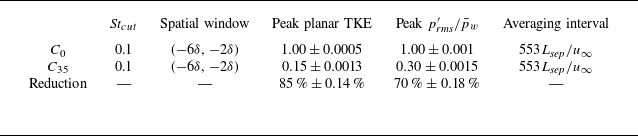
). Within the bump region, the TKE drops to a minimum near the bump peak before increasing again downstream. The peak TKE value in the controlled interaction is approximately 0.15, which is considerably lower than that of the uncontrolled case. Details of this reduction in peak values are presented in table 2. Furthermore, the control effects are independent of the spanwise width, as confirmed by a wider case (
$b$
). Within the bump region, the TKE drops to a minimum near the bump peak before increasing again downstream. The peak TKE value in the controlled interaction is approximately 0.15, which is considerably lower than that of the uncontrolled case. Details of this reduction in peak values are presented in table 2. Furthermore, the control effects are independent of the spanwise width, as confirmed by a wider case ( $8\delta$
) presented in Appendix A.
$8\delta$
) presented in Appendix A.
Performance metrics. For easy comparison, both TKE and $p^{\prime}_{\textit{rms}} /\bar {p}_{w}$
are normalised by the peak values in case
$p^{\prime}_{\textit{rms}} /\bar {p}_{w}$
are normalised by the peak values in case $C_{0}$
.
$C_{0}$
.

The control effect is also reflected in the wall-pressure fluctuations $ p^{\prime}_{\textit{rms}}/\bar {p}_{w}$
in figure 4(
$ p^{\prime}_{\textit{rms}}/\bar {p}_{w}$
in figure 4( $f$
). The
$f$
). The $C_{0}$
case displays a single, prominent peak near
$C_{0}$
case displays a single, prominent peak near $x_{\textit{sep}}$
, which decays rapidly downstream and plateaus at around 0.25. The
$x_{\textit{sep}}$
, which decays rapidly downstream and plateaus at around 0.25. The $C_{35}$
case, however, exhibits a bifurcated response with two distinct peaks: one of magnitude 0.15 associated with the upstream separation, and a second peak of 0.3 near the bump peak. Critically, both peaks are substantially weaker than the dominant peak in the uncontrolled flow. Downstream of the bump, the
$C_{35}$
case, however, exhibits a bifurcated response with two distinct peaks: one of magnitude 0.15 associated with the upstream separation, and a second peak of 0.3 near the bump peak. Critically, both peaks are substantially weaker than the dominant peak in the uncontrolled flow. Downstream of the bump, the $ p^{\prime}_{\textit{rms}}/\bar {p}_{w}$
values stabilise at a level comparable to the uncontrolled case.
$ p^{\prime}_{\textit{rms}}/\bar {p}_{w}$
values stabilise at a level comparable to the uncontrolled case.
Our results confirm that the micro-bump significantly attenuates the low-frequency breathing motion. The control mechanism operates by minimally modifying the base flow, which stabilises the dominant 2-D shock mode and thereby makes it more difficult to be excited by external disturbances. Another plausible explanation is the transformation of the separation mechanism from pressure-induced separation to geometry-induced separation, the latter being associated with comparatively weaker low-frequency dynamics due to the relatively fixed separation point (Eaton & Johnston Reference Eaton and Johnston1982; Borgmann et al. Reference Borgmann, Cura, Weiss and Little2024).
Comparisons of ( $a$
) pre-multiplied wall-pressure spectra, (
$a$
) pre-multiplied wall-pressure spectra, ( $b$
) integrated planar TKE (
$b$
) integrated planar TKE ( $ \textit{St}_{cut}=0.1$
) and (
$ \textit{St}_{cut}=0.1$
) and ( $c$
) the maximum growth rate of the 2-D mode for cases with different bump heights. Streamwise stations in (
$c$
) the maximum growth rate of the 2-D mode for cases with different bump heights. Streamwise stations in ( $a$
):
$a$
): $x_{\textit{sep}}$
for uncontrolled case and
$x_{\textit{sep}}$
for uncontrolled case and $x_{p}$
for controlled cases.
$x_{p}$
for controlled cases.

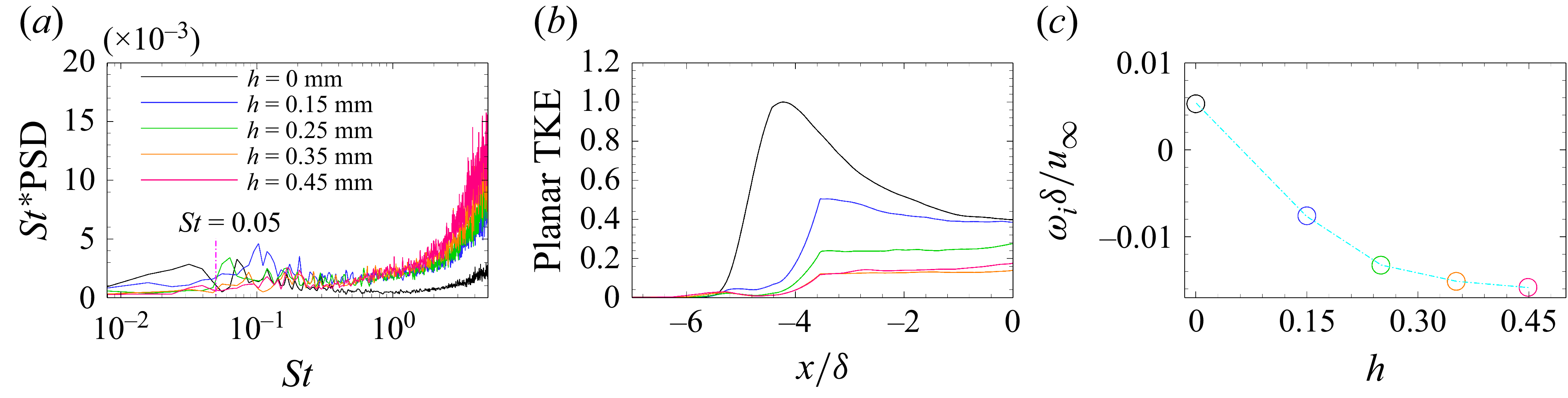
Effects of bump height are then investigated. Figure 5( $a$
) compares the pre-multiplied wall-pressure spectra for cases with different heights. The low-frequency peak diminishes at
$a$
) compares the pre-multiplied wall-pressure spectra for cases with different heights. The low-frequency peak diminishes at $h=0.15$
mm, indicating that the bump begins to effectively suppress the breathing motion at this height. The low-frequency TKE level drops sharply compared with the uncontrolled case
$h=0.15$
mm, indicating that the bump begins to effectively suppress the breathing motion at this height. The low-frequency TKE level drops sharply compared with the uncontrolled case $C_{0}$
, as seen in figure 5(
$C_{0}$
, as seen in figure 5( $b$
). Further increasing the bump height has little influence on the spectral shape, but the TKE level continues to decline with height up to
$b$
). Further increasing the bump height has little influence on the spectral shape, but the TKE level continues to decline with height up to $h = 0.35$
mm. At
$h = 0.35$
mm. At $h = 0.45$
mm, the TKE level is comparable to that at
$h = 0.45$
mm, the TKE level is comparable to that at $h = 0.35$
mm, suggesting a local weakening of the suppressive effects. The weakening effects can be explained using the maximum growth rates of the 2-D mode, as illustrated in figure 5(
$h = 0.35$
mm, suggesting a local weakening of the suppressive effects. The weakening effects can be explained using the maximum growth rates of the 2-D mode, as illustrated in figure 5( $c$
). The growth rate decreases monotonically with bump height, a trend that tends to saturate around
$c$
). The growth rate decreases monotonically with bump height, a trend that tends to saturate around $h = 0.45$
mm. In the presence of a bump, the mode shape resembles that shown in figure 4(
$h = 0.45$
mm. In the presence of a bump, the mode shape resembles that shown in figure 4( $b$
). As noted earlier, modal resonance can excite the 2-D mode, which is linked to the weakened breathing motion and can be triggered under modal resonance. Therefore, a sharp reduction in fluctuating energy results from a significantly damped growth rate. If the bump height is increased further, the flow may no longer remain only slightly disturbed and nonlinear effects could emerge, which might in turn reduce the effectiveness of the suppression mechanism.
$b$
). As noted earlier, modal resonance can excite the 2-D mode, which is linked to the weakened breathing motion and can be triggered under modal resonance. Therefore, a sharp reduction in fluctuating energy results from a significantly damped growth rate. If the bump height is increased further, the flow may no longer remain only slightly disturbed and nonlinear effects could emerge, which might in turn reduce the effectiveness of the suppression mechanism.
Comparisons of ( $a{,} b$
)
$a{,} b$
) $C_{f}$
and
$C_{f}$
and $C_{p}$
, (
$C_{p}$
, ( $c$
) pre-multiplied wall-pressure spectra, (
$c$
) pre-multiplied wall-pressure spectra, ( $d$
) integrated planar TKE (
$d$
) integrated planar TKE ( $ \textit{St}_{cut}=0.1$
) and (
$ \textit{St}_{cut}=0.1$
) and ( $e$
) the normalised wall-pressure root mean square (
$e$
) the normalised wall-pressure root mean square ( $ \textit{St}_{cut}=0.1$
) of cases at different positions.
$ \textit{St}_{cut}=0.1$
) of cases at different positions.

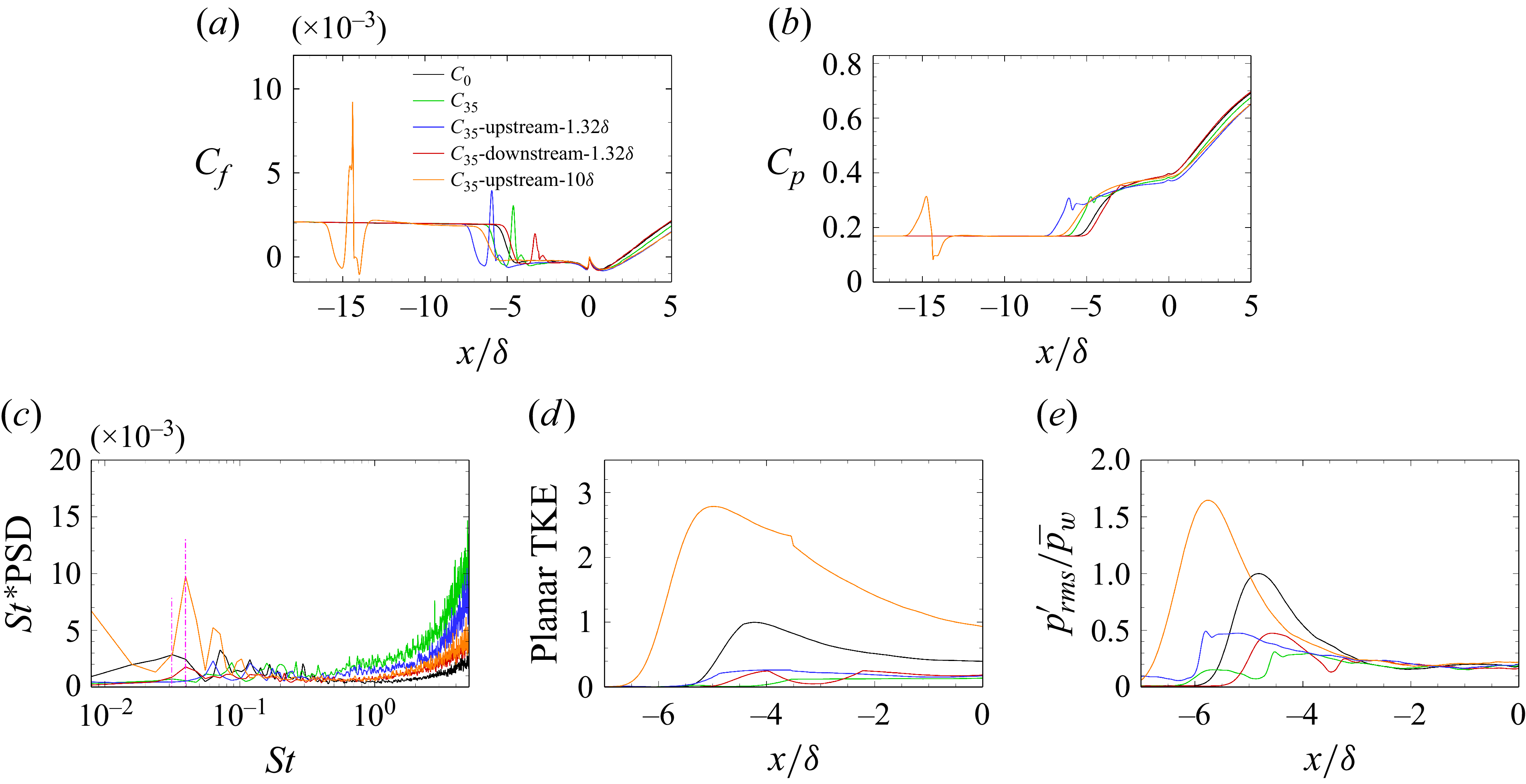
The effects of bump position are examined by considering three additional cases: case $C_{35}$
–upstream–1.32
$C_{35}$
–upstream–1.32 $\delta$
, with the bump shifted
$\delta$
, with the bump shifted $1.32\delta$
upstream;
$1.32\delta$
upstream; $C_{35}$
–downstream–1.32
$C_{35}$
–downstream–1.32 $\delta$
, with the bump shifted
$\delta$
, with the bump shifted $1.32\delta$
downstream; and case
$1.32\delta$
downstream; and case $C_{35}$
–upstream–10
$C_{35}$
–upstream–10 $\delta$
, with the bump shifted
$\delta$
, with the bump shifted $10\delta$
upstream. The first two cases are designed to assess the impact of slight bump shifts, whereas the last case represents a fully off-design condition. Figure 6(
$10\delta$
upstream. The first two cases are designed to assess the impact of slight bump shifts, whereas the last case represents a fully off-design condition. Figure 6( $a{,} b$
) compares the distributions of
$a{,} b$
) compares the distributions of $C_{f}$
and
$C_{f}$
and $C_{p}$
for cases at different positions. Large separation bubbles are formed in the two upstream cases, whereas the downstream bump, concealed within the separation bubble, induces only minor changes in the two distributions relative to case
$C_{p}$
for cases at different positions. Large separation bubbles are formed in the two upstream cases, whereas the downstream bump, concealed within the separation bubble, induces only minor changes in the two distributions relative to case $C_{0}$
. Figure 6(
$C_{0}$
. Figure 6( $c$
) shows the pre-multiplied wall-pressure spectra for the original
$c$
) shows the pre-multiplied wall-pressure spectra for the original $C_{0}$
and
$C_{0}$
and $C_{35}$
cases, together with the three repositioned cases. The low-frequency peak is greatly amplified for the fully off-design case (
$C_{35}$
cases, together with the three repositioned cases. The low-frequency peak is greatly amplified for the fully off-design case ( $C_{35}$
–upstream–10
$C_{35}$
–upstream–10 $\delta$
). For the two slightly shifted cases, the low-frequency components are enhanced compared with the well-controlled
$\delta$
). For the two slightly shifted cases, the low-frequency components are enhanced compared with the well-controlled $C_{35}$
case, although both remain slightly lower than that in case
$C_{35}$
case, although both remain slightly lower than that in case $C_{0}$
. The peak TKE and
$C_{0}$
. The peak TKE and $ p^{\prime}_{\textit{rms}}/\bar {p}_{w}$
values increase by 300
$ p^{\prime}_{\textit{rms}}/\bar {p}_{w}$
values increase by 300 $\,\%$
and 150
$\,\%$
and 150 $\,\%$
, respectively, in the
$\,\%$
, respectively, in the $C_{35}$
–upstream–10
$C_{35}$
–upstream–10 $\delta$
case. In contrast, the two slightly shifted cases show similar satisfactory reductions in the shock motion strength, with decreases of approximately
$\delta$
case. In contrast, the two slightly shifted cases show similar satisfactory reductions in the shock motion strength, with decreases of approximately $75\,\%$
in the peak TKE and
$75\,\%$
in the peak TKE and $50\,\%$
in
$50\,\%$
in $ p^{\prime}_{\textit{rms}}/\bar {p}_{w}$
.
$ p^{\prime}_{\textit{rms}}/\bar {p}_{w}$
.
The conclusions drawn here regarding positioning the bump far upstream are consistent with Della Posta et al. (Reference Della Posta, Martelli, Salvadore and Bernardini2024), who reported that an upstream vortex generator amplified the low-frequency magnitude of shock motion. The two partially off-design conditions suggest that slight shifts of the bump can still mitigate the unsteadiness, although the effectiveness varies. Further efforts could employ techniques such as piezoelectrics and shape memory alloys to advance this control strategy towards practical implementation, ensuring the bump remains in the effective region across varying flow conditions.
4. Conclusions
This study employs a micro-bump to suppress the low-frequency unsteadiness in STBLIs through LES and stability analysis. The unsteadiness is shown to be driven by a 2-D global mode, whose instability originates primarily from the shock-foot region. By positioning a micro-bump at this critical region, the 2-D global mode is effectively damped and the local flow dynamics is altered, which substantially weakens the low-frequency motion. The controlled wall-pressure spectrum shows that the energy peak at $ \textit{St}\lt 0.05$
vanishes, leading to reductions of 85
$ \textit{St}\lt 0.05$
vanishes, leading to reductions of 85 $\,\%$
in TKE and 70
$\,\%$
in TKE and 70 $\,\%$
in wall-pressure fluctuations associated with
$\,\%$
in wall-pressure fluctuations associated with $ \textit{St}\lt 0.1$
. These findings highlight the effectiveness of using a micro-bump to mitigate low-frequency unsteadiness, achieving precise suppression with negligible disturbance to the flow and minimal additional drag or other aerodynamic penalties.
$ \textit{St}\lt 0.1$
. These findings highlight the effectiveness of using a micro-bump to mitigate low-frequency unsteadiness, achieving precise suppression with negligible disturbance to the flow and minimal additional drag or other aerodynamic penalties.
The effects of bump height and position are investigated. Effective suppression of breathing motion is achieved once the bump height exceeds $h=0.15$
mm, and the control effect saturates beyond
$h=0.15$
mm, and the control effect saturates beyond $h=0.35$
mm. Furthermore, slightly adjusting the bump position weakens the suppression effects but does not exacerbate the unsteadiness, provided the bump is located near the separation point. These observations may provide useful guidance for practical implementations.
$h=0.35$
mm. Furthermore, slightly adjusting the bump position weakens the suppression effects but does not exacerbate the unsteadiness, provided the bump is located near the separation point. These observations may provide useful guidance for practical implementations.
Supplementary movies
Supplementary movies are available at https://doi.org/10.1017/jfm.2026.11679.
Acknowledgements
The authors thank Professor J. Weiss for helpful discussions.
Funding
This work was supported by the National Natural Science Foundation of China under grant 12472239 and the Hong Kong Research Grants Council under grant 15204322.
Declaration of interests
The authors report no conflict of interest.
Appendix A. Effects of the computational width
Case $C_{0}$
: (
$C_{0}$
: ( $a$
) real part of the leading 2-D SPOD mode at
$a$
) real part of the leading 2-D SPOD mode at $ St=0.023$
from the wide case (
$ St=0.023$
from the wide case ( $15\delta$
) and (
$15\delta$
) and ( $b$
) wall-normal integrated planar TKE (
$b$
) wall-normal integrated planar TKE ( $ \textit{St}_{cut}=0.1$
) from the original and wide cases, normalised by their respective maxima. Case
$ \textit{St}_{cut}=0.1$
) from the original and wide cases, normalised by their respective maxima. Case $C_{35}$
: (
$C_{35}$
: ( $c$
) Pre-multiplied wall-pressure spectra and (
$c$
) Pre-multiplied wall-pressure spectra and ( $d$
) planar TKE (
$d$
) planar TKE ( $ \textit{St}_{cut}=0.1$
) at different widths (
$ \textit{St}_{cut}=0.1$
) at different widths ( $4\delta$
and
$4\delta$
and $8\delta$
), normalised by their respective maxima. (
$8\delta$
), normalised by their respective maxima. ( $e$
) The comparison of eigenvalues for cases
$e$
) The comparison of eigenvalues for cases $C_{0}$
and
$C_{0}$
and $C_{35}$
at different widths.
$C_{35}$
at different widths.

The effects of computational width are examined in this appendix. For the uncontrolled $C_{0}$
case, while the present width cannot resolve large-scale spanwise structures of the order of twice the separation length (Ceci et al. Reference Ceci, Palumbo, Larsson and Pirozzoli2023; Zhang et al. Reference Zhang, Li and Hao2025b
), it is sufficient to capture the dominant 2-D dynamics (Grilli et al. Reference Grilli, Schmid, Hickel and Adams2012; Priebe et al. Reference Priebe, Tu, Rowley and Martín2016; Pasquariello et al. Reference Pasquariello, Hickel and Adams2017). To verify that the 2-D dynamics is independent of the computational domain width, we compare the original case (spanwise width
$C_{0}$
case, while the present width cannot resolve large-scale spanwise structures of the order of twice the separation length (Ceci et al. Reference Ceci, Palumbo, Larsson and Pirozzoli2023; Zhang et al. Reference Zhang, Li and Hao2025b
), it is sufficient to capture the dominant 2-D dynamics (Grilli et al. Reference Grilli, Schmid, Hickel and Adams2012; Priebe et al. Reference Priebe, Tu, Rowley and Martín2016; Pasquariello et al. Reference Pasquariello, Hickel and Adams2017). To verify that the 2-D dynamics is independent of the computational domain width, we compare the original case (spanwise width $4\delta$
) with a wider case (
$4\delta$
) with a wider case ( $15\delta$
), which includes large-scale 3-D spanwise undulations. As shown in figure 7(
$15\delta$
), which includes large-scale 3-D spanwise undulations. As shown in figure 7( $a$
), the leading SPOD mode at
$a$
), the leading SPOD mode at $ \textit{St}=0.023$
for the wide case closely resembles the mode in figure 1(
$ \textit{St}=0.023$
for the wide case closely resembles the mode in figure 1( $b$
). Furthermore, figure 7(
$b$
). Furthermore, figure 7( $b$
) shows that the streamwise distributions of the integrated TKE are nearly identical between the two cases. These comparisons confirm that extending the spanwise width does not alter the fundamental characteristics of the 2-D dynamics.
$b$
) shows that the streamwise distributions of the integrated TKE are nearly identical between the two cases. These comparisons confirm that extending the spanwise width does not alter the fundamental characteristics of the 2-D dynamics.
For the controlled case $C_{35}$
, a wider domain (
$C_{35}$
, a wider domain ( $8\delta$
) is considered. Figures 7(
$8\delta$
) is considered. Figures 7( $c$
) and 7(
$c$
) and 7( $d$
) compare the pre-multiplied PSD distributions and the integrated planar TKE profiles between cases with different widths, respectively. The good agreement indicates that the domain width does not influence the control effects. Moreover, the comparison of eigenvalues for cases
$d$
) compare the pre-multiplied PSD distributions and the integrated planar TKE profiles between cases with different widths, respectively. The good agreement indicates that the domain width does not influence the control effects. Moreover, the comparison of eigenvalues for cases $C_{0}$
and
$C_{0}$
and $C_{35}$
with different widths is shown in figure 7(
$C_{35}$
with different widths is shown in figure 7( $e$
). As expected, variations in width have only a minor influence on the leading few eigenvalues. The impact of the bump on 3-D modes will be addressed in a future study.
$e$
). As expected, variations in width have only a minor influence on the leading few eigenvalues. The impact of the bump on 3-D modes will be addressed in a future study.
Appendix B. Eddy viscosity $\boldsymbol{\mu _{t}}$

The Boussinesq assumption gives
 \begin{align} -\rho \big \langle u_{i}^{\prime\prime} u_{j}^{\prime\prime} \big \rangle =-\frac {2}{3} \rho K\delta _{\textit{ij}} +\left(-\frac {2}{3}\mu _{t}S_{kk} \delta _{\textit{ij}}+2\mu _{t}S_{\textit{ij}} \right)\quad (i,j,k\in \left \{ 1,2,3 \right \} ), \end{align}
where $K$
is the total TKE,
$K$
is the total TKE, $S$
is the Favre-averaged strain-rate tensor and
$S$
is the Favre-averaged strain-rate tensor and $\delta _{\textit{ij}}$
is the Kronecker delta. Letting
$\delta _{\textit{ij}}$
is the Kronecker delta. Letting $L_{\textit{ij}}= -\rho \langle u_{i}^{\prime\prime} u_{j}^{\prime\prime} \rangle +2/3 \rho K\delta _{\textit{ij}}$
and
$L_{\textit{ij}}= -\rho \langle u_{i}^{\prime\prime} u_{j}^{\prime\prime} \rangle +2/3 \rho K\delta _{\textit{ij}}$
and $M_{\textit{ij}}=-1/3S_{kk} \delta _{\textit{ij}}+S_{\textit{ij}}$
, the square of the error in (B1) can be defined as (Lilly Reference Lilly1992)
$M_{\textit{ij}}=-1/3S_{kk} \delta _{\textit{ij}}+S_{\textit{ij}}$
, the square of the error in (B1) can be defined as (Lilly Reference Lilly1992)
 \begin{align} Q= \big(L_{\textit{ij}}-2\mu _{t}M_{\textit{ij}} \big)^{2}. \end{align}
Upon setting $\partial Q/ \partial \mu _{t}=0$
,
$\partial Q/ \partial \mu _{t}=0$
, $\mu _{t}$
is evaluated as
$\mu _{t}$
is evaluated as
 \begin{align} \mu _{t}=\frac {1}{2} \big(L_{\textit{ij}}M_{\textit{ij}}/M_{\textit{ij}}^{2} \big), \end{align}
which represents the minimum of $Q$
. The least-squares fitting method has been adopted by Abe et al. (Reference Abe, Mizobuchi, Matsuo and Spalart2012), Coleman, Rumsey & Spalart (Reference Coleman, Rumsey and Spalart2018) and Zhang et al. (Reference Zhang, Li and Hao2025b
). Regarding the robustness of
$Q$
. The least-squares fitting method has been adopted by Abe et al. (Reference Abe, Mizobuchi, Matsuo and Spalart2012), Coleman, Rumsey & Spalart (Reference Coleman, Rumsey and Spalart2018) and Zhang et al. (Reference Zhang, Li and Hao2025b
). Regarding the robustness of $\mu _{t}$
in stability analysis, Pickering et al. (Reference Pickering, Rigas, Schmidt, Sipp and Colonius2021) and Fan et al. (Reference Fan, Kozul, Li and Sandberg2024) systematically discussed different
$\mu _{t}$
in stability analysis, Pickering et al. (Reference Pickering, Rigas, Schmidt, Sipp and Colonius2021) and Fan et al. (Reference Fan, Kozul, Li and Sandberg2024) systematically discussed different $\mu _{t}$
strategies in resolvent analysis and concluded that the optimal mode is insensitive to the relatively small differences in
$\mu _{t}$
strategies in resolvent analysis and concluded that the optimal mode is insensitive to the relatively small differences in $\mu _{t}$
when it is represented properly. Hao (Reference Hao2023) demonstrated that although varying RANS models changes the most unstable eigenvalues, the leading modal structures remain consistent. To verify this insensitivity, an alternative
$\mu _{t}$
when it is represented properly. Hao (Reference Hao2023) demonstrated that although varying RANS models changes the most unstable eigenvalues, the leading modal structures remain consistent. To verify this insensitivity, an alternative $\mu _{t}$
field can be represented using the following formula:
$\mu _{t}$
field can be represented using the following formula:
 \begin{align} \mu _{t} =C_{\mu }\rho \frac {K^{2} }{\epsilon }, \end{align}
where $C_{\mu }=0.09$
and
$C_{\mu }=0.09$
and $\epsilon$
is the rate of dissipation of TKE (Pope Reference Pope2001). The corresponding shock mode and sensitivity analysis results are presented in figure 8. The resulting mode shape is qualitatively consistent with that shown in figure 1(
$\epsilon$
is the rate of dissipation of TKE (Pope Reference Pope2001). The corresponding shock mode and sensitivity analysis results are presented in figure 8. The resulting mode shape is qualitatively consistent with that shown in figure 1( $a$
), and the most sensitive region remains concentrated around the shock foot, aligning with the observations in figure 2(
$a$
), and the most sensitive region remains concentrated around the shock foot, aligning with the observations in figure 2( $a$
). These comparisons confirm that the linear dynamics is relatively robust with respect to the specific choice of
$a$
). These comparisons confirm that the linear dynamics is relatively robust with respect to the specific choice of $\mu _{t}$
.
$\mu _{t}$
.
( $a$
) Shock mode and (
$a$
) Shock mode and ( $b$
) sensitivity analysis results obtained using the alternative eddy-viscosity model (
$b$
) sensitivity analysis results obtained using the alternative eddy-viscosity model ( $\mu _{t} =C_{\mu }\rho K^{2} /\epsilon$
).
$\mu _{t} =C_{\mu }\rho K^{2} /\epsilon$
).

Appendix C. Convergence analysis of SPOD
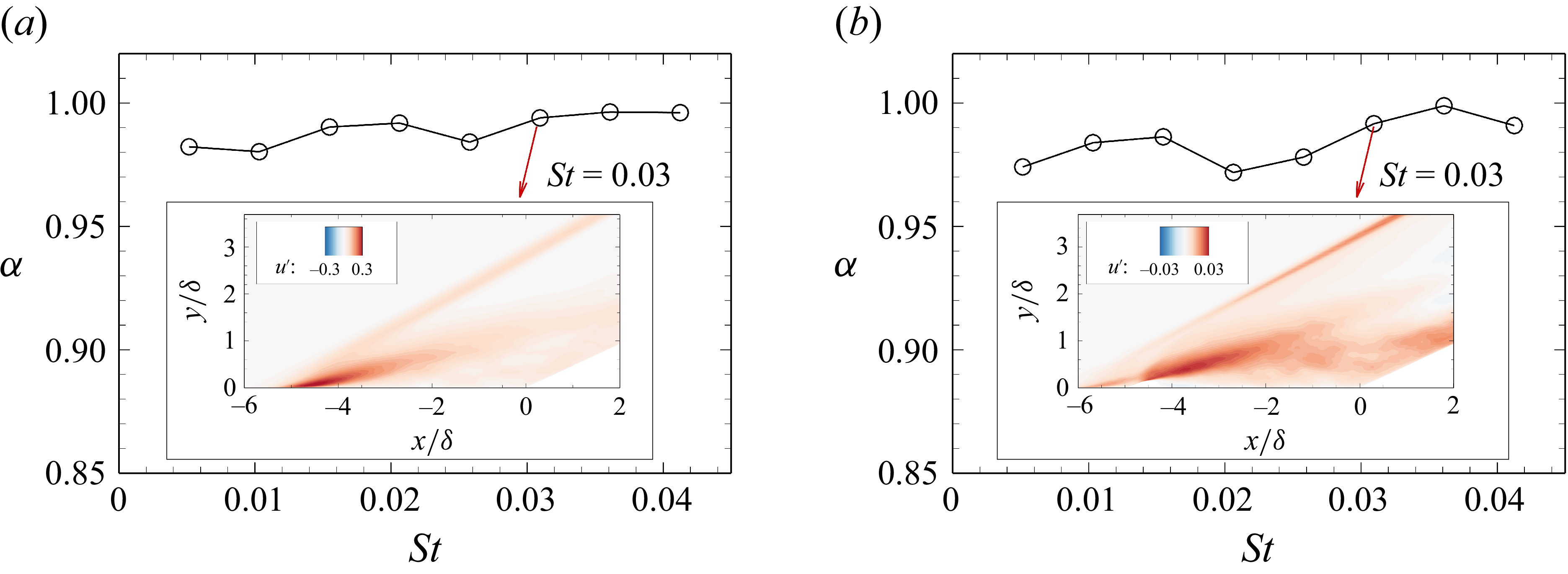
This appendix aims to verify the convergence of the SPOD modes. Convergence is highly correlated with the number of samples (Lesshafft et al. Reference Lesshafft, Semeraro, Jaunet, Cavalieri and Jordan2019; Schmidt & Colonius Reference Schmidt and Colonius2020). Accordingly, the correlation coefficient $\alpha$
is defined as (Abreu et al. Reference Abreu, Cavalieri, Schlatter, Vinuesa and Henningson2020; Zhang et al. Reference Zhang, Hao and Uy2025a
)
$\alpha$
is defined as (Abreu et al. Reference Abreu, Cavalieri, Schlatter, Vinuesa and Henningson2020; Zhang et al. Reference Zhang, Hao and Uy2025a
)
 \begin{align} \alpha =\frac {\left | {\parallel \boldsymbol{{\varPsi }_{100\,\%}}, \boldsymbol{{\varPsi }_{75\,\%}}\parallel }_{E} \right |}{ {\parallel \boldsymbol{{\varPsi }_{100\,\%}}\parallel }_{E} \times {\parallel \boldsymbol{{\varPsi }_{75\,\%}}\parallel }_{E} }, \end{align}
where $ \boldsymbol{\varPsi }$
denotes the leading SPOD modes of the first nine frequencies and the subscripts ‘
$ \boldsymbol{\varPsi }$
denotes the leading SPOD modes of the first nine frequencies and the subscripts ‘ $100\,\%$
’ and ‘
$100\,\%$
’ and ‘ $75\,\%$
’ indicate the dataset length. A value of 1 indicates a perfect match between the modes from different datasets. Figure 9(
$75\,\%$
’ indicate the dataset length. A value of 1 indicates a perfect match between the modes from different datasets. Figure 9( $a{,} b$
) presents the coefficients from cases
$a{,} b$
) presents the coefficients from cases $C_{0}$
and
$C_{0}$
and $C_{35}$
. For all frequencies, values of
$C_{35}$
. For all frequencies, values of $\alpha \gt 0.97$
are obtained. The streamwise velocity perturbations as shown in the insets in figure 9(
$\alpha \gt 0.97$
are obtained. The streamwise velocity perturbations as shown in the insets in figure 9( $a{,} b$
) closely resemble those in figures 1(
$a{,} b$
) closely resemble those in figures 1( $a$
) and 4(
$a$
) and 4( $c$
). The results based on the 75
$c$
). The results based on the 75 $\,\%$
subset show excellent agreement with those from the full 100
$\,\%$
subset show excellent agreement with those from the full 100 $\,\%$
dataset. Hence, the SPOD modes are regarded as converged.
$\,\%$
dataset. Hence, the SPOD modes are regarded as converged.
Convergence analysis of ( $a$
) case
$a$
) case $C_{0}$
and (
$C_{0}$
and ( $b$
) case
$b$
) case $C_{35}$
. The insets are from the 75
$C_{35}$
. The insets are from the 75 $\,\%$
dataset.
$\,\%$
dataset.















 Open access

