


I. Introduction
Plant protection is an essential component of agricultural production, with numerous systems relying on synthetic pesticides (Savary et al., Reference Savary, Willocquet, Pethybridge, Esker, McRoberts and Nelson2019). However, their widespread and intensive application has been associated with harmful effects on the environment and human health (Tang et al., Reference Tang, Lenzen, McBratney and Maggi2021). Consequently, reductions of pesticide use and risk have become pivotal components of agricultural policies, particularly in Europe (Schneider et al., Reference Schneider, Barreiro-Hurle and Rodriguez-Cerezo2023). Grapevine is among the crops with the highest pesticide usage (Fouillet et al., Reference Fouillet, Delière, Chartier, Munier-Jolain, Cortel, Rapidel and Merot2022). It requires between 12 and 15 pesticide applications per year alone, making up a vast share of pesticide use in EuropeFootnote 1 and Switzerland.Footnote 2 Given its substantial potential for reduction, grapevine is imperative in achieving pesticide reduction goals. However, this potential has not been fully realized. A range of pesticide reduction measures are available to winegrowers and combining these is needed to meet pesticide reduction policy goals (see e.g., Finger et al., Reference Finger, Sok, Ahovi, Akter, Bremmer, Dachbrodt-Saaydeh, de Lauwere, Kreft, Kudsk, Lambarraa-Lehnhardt, McCallum, Lansink, Wauters and Möhring2024). Assessment of practice adoption however frequently happens in isolation, so little is known about specific measure combinations most frequently used, and the factors influencing such a bundled adoption (e.g., Chen et al., Reference Chen, Herrera, Benitez, Hoffmann, Möth, Paredes, Plaas, Popescu, Rascher, Rusch, Sandor, Tolle, Willemen, Winter and Schwarz2022).
To address this knowledge gap, we conduct a comprehensive assessment of a large collection of pesticide reduction measures, using survey data from 436 Swiss grape growers (Zachmann et al., Reference Zachmann, McCallum and Finger2023b). The objective of this study is twofold: first, to identify links between the adoption of individual measures (i.e., within each pesticide category), and second, to examine how individual measures are combined to form global pesticide reduction strategies across pesticide categories. In addition, the study assesses how measure, farm, and farmer characteristics are associated with the adoption of both individual and bundles of measures.
A substantial body of literature exists on the adoption of sustainable crop protection practices (e.g., Möhring et al., Reference Möhring, Ingold, Kudsk, Martin-Laurent, Niggli, Siegrist, Studer, Walter and Finger2020a). For viticulture, many studies focus on specific strategies in isolation, such as preventative measures (Wang and Finger, Reference Wang and Finger2023), precision application technologies (Wandkar et al., Reference Wandkar, Bhatt, Jain, Nalawade and Pawar2018), or the adoption of resistant varieties (Finger et al., Reference Finger, Zachmann and McCallum2023). The assessment of multiple measures as part of bundles however is highly relevant due to the higher efficacy of bundles and their relevance in achieving sustainable pesticide reduction (e.g., Finger et al., Reference Finger, Sok, Ahovi, Akter, Bremmer, Dachbrodt-Saaydeh, de Lauwere, Kreft, Kudsk, Lambarraa-Lehnhardt, McCallum, Lansink, Wauters and Möhring2024). Additionally, individual measures may not be independent from each other, for example due to technical exclusion (Gagliardi et al., Reference Gagliardi, Fontanelli, Luglio, Frasconi, Peruzzi and Raffaelli2023) or complementary effects (Reiff et al., Reference Reiff, Ehringer, Hoffmann and Entling2021). The consideration of bundles also holds relevance for the targeted design of effective support policies (e.g., Fouillet et al., Reference Fouillet, Delière, Flori, Rapidel and Merot2023; Ghali et al., Reference Ghali, Ben Jaballah, Ben Arfa and Sigwalt2022). However, evaluations of farmer decision-making surrounding pesticide reduction that explicitly consider measure bundles are currently lacking.
We address this research gap by providing a detailed assessment of adoption patterns for 21 pesticide reduction strategies in Swiss viticulture, using survey data from 436 farms. We utilize a contingency analysis to assess which measures are more likely to be used as part of bundles, and a k-means clustering algorithm to identify how pest management strategies differ across our dataset. We further use regression analysis to identify which farm and farmer characteristics, behavioral factors, and environmental influences are relevant determinants in shaping adoption of different strategies.
Our findings indicate that capital and labor constraints are important determinants for measure occurrence in bundles, but that complementary effects between measures are also highly relevant in shaping their joint or separate adoption. The k-means analysis reveals that half of Swiss grape growers currently implement a broad variety of pesticide reduction measures, while the other half tends to rely primarily on the use of pesticides. The clusters are labeled “Low-IPM” (52% of growers) and “High-IPM” (48% of growers), with reference to their adoption levels of integrated pest management (IPM) practices. We identify notable differences in farm and farmer characteristics between both clusters, and use a logit regression model to identify the statistical significance of these differences. Results indicate that some structural and demographic characteristics such as marketing wine, having completed an agricultural apprenticeship, and producing in accordance with ecological cross-compliance significantly increase the probability of being a High-IPM-Adopter. Additionally, behavioral factors matter, for example, non-cognitive skills, risk preferences, and farmer goals and self-identity. Based on our findings, we make several detailed policy recommendations, to be used to design more effective and efficient policies to incentivize the adoption of pesticide reduction measures among current Low-IPM-Adopters. Our analysis thus contributes to a more holistic understanding of farmer choices of pesticide reduction measures and thus supports decision-making by farmers, industry and policymakers, also beyond viticulture, and beyond the case study of Switzerland.
The remainder of this paper is structured as follows. Section II provides information on the study background and conceptual framework, Section III covers the methods and data, Section IV presents the results, which are then discussed in Section V, before concluding with Section VI.
II. Background and conceptual framework
Pesticide reduction measures and their characteristics. Various pesticide reduction measures exist for viticulture (see, e.g., Pertot et al., Reference Pertot, Caffi, Rossi, Mugnai, Hoffmann, Grando, Gary, Lafond, Duso, Thiery, Mazzoni and Anfora2017). These include the substitution of synthetic fungicides and copperFootnote 3, for example with microorganisms, or inorganic compounds, the replacement of synthetic herbicides using mechanical weeding or mulching, or alternatives to synthetic insecticides using mechanical nets and traps. Disease pressure may also be mitigated through preventative measures, such as sanitation, canopy management, or controlled fertilizer use (Pertot et al., Reference Pertot, Caffi, Rossi, Mugnai, Hoffmann, Grando, Gary, Lafond, Duso, Thiery, Mazzoni and Anfora2017). Furthermore, the necessity of pesticide applications may be lowered altogether, for instance through the use of decision support tools (e.g., forecasting systems), by replanting traditional varieties with less susceptible alternatives (i.e., fungus-resistant varieties) (Finger et al., Reference Finger, Zachmann and McCallum2023), or by promoting beneficial insects to control harmful pest populations (Reiff et al., Reference Reiff, Sudarsan, Hoffmann and Entling2023). Lastly, precision application technologies can enhance the efficiency of conventional pesticide applications by reducing drift and run-off.
Table 1 gives an overview of all pesticide reduction measures included in the survey and analysis. The data contains binary adoption data (1 = use of measure, 0 = non-use of measure) for both conventional pesticide use as well as pesticide reduction measures (see Zachmann et al., Reference Zachmann, McCallum and Finger2023b for details). In total, the sample contains information on 15 pesticide reduction measures, and 6 precision application technologies, yielding 21 total measures included in our analysis.
Overview of pesticide reduction measures in the sample. For a detailed overview of evaluation criteria and additional insights into each measure, see Appendix, Section 1 for further details

Note: Participation numbers taken from survey data (Zachmann et al., Reference Zachmann, McCallum and Finger2023b). Throughout the analysis, the dimension value of increases or decreases in capital- and labor-intensity is indicated through a proxy ratingFootnote 4, ranging rom ↑/↓ (low), ↑↑/↓ ↓ (moderate), and ↑↑↑/ ↓ ↓ ↓ (high). An estimation of the reduction potential within each pesticide category is also given. All ratings rely on related literature (e.g., Fouillet et al., Reference Fouillet, Delière, Chartier, Munier-Jolain, Cortel, Rapidel and Merot2022; Pertot et al., Reference Pertot, Caffi, Rossi, Mugnai, Hoffmann, Grando, Gary, Lafond, Duso, Thiery, Mazzoni and Anfora2017).
Four dimensions are crucial to characterize pesticide reduction measures (see e.g., Chen et al., Reference Chen, Herrera, Benitez, Hoffmann, Möth, Paredes, Plaas, Popescu, Rascher, Rusch, Sandor, Tolle, Willemen, Winter and Schwarz2022; Wang et al., Reference Wang, Möhring and Finger2023): capital-intensity, labor-intensity, pesticide reduction potential, and the associated time lag between measure implementation and effect (Table 1). The first two dimensions are of particular significance due to the high capital and labor requirements inherent to viticulture. For example, Swiss vineyards frequently feature inclines, requiring between 450 and 800 labor-hours per hectare and year (Höper et al., Reference Höper, Zachmann and Finger2025). Capital-intensive practices describe measures that are assumed to be more costly than conventional pesticides on average. These higher costs may arise from significant upfront investments or recurring seasonal costs, which are often higher for pesticide alternatives due to the underdeveloped state of their markets and the lower effectiveness of such alternatives, requiring more frequent applications (Pertot et al., Reference Pertot, Caffi, Rossi, Mugnai, Hoffmann, Grando, Gary, Lafond, Duso, Thiery, Mazzoni and Anfora2017). Higher labor requirements may happen because measures increase the workload directly (e.g., lower effectiveness than conventional pesticides, or relying on manual labor), or due to labor associated with correct measure implementation (e.g., information gathering, measure timing, etc.) (Pertot et al., Reference Pertot, Caffi, Rossi, Mugnai, Hoffmann, Grando, Gary, Lafond, Duso, Thiery, Mazzoni and Anfora2017).
The time-lag associated with measures is another important factor for decision-making. We define measures without a time lag as those with immediate effects, while lagged measures are characterized by a time lag between implementation control effect. In general, such a time lag has been shown to hinder practice adoption for impatient farmers. Moreover, such measures may be less attractive for risk averse farmers because their upfront investment in capital and labor occurs uncertain, as their benefit depends on the occurrence of pathogen presence later in the growing season (Wang and Finger, Reference Wang and Finger2023).
Finally, while capital intensity, labor intensity, and associated time lag have been demonstrated to influence measure adoption (see Chen et al., Reference Chen, Herrera, Benitez, Hoffmann, Möth, Paredes, Plaas, Popescu, Rascher, Rusch, Sandor, Tolle, Willemen, Winter and Schwarz2022), the pesticide reduction potential of a measure is ultimately determinative of its impact on policy goals. Measures with a substantial reduction potentialFootnote 5 can greatly reduce the use of pesticides (e.g., 80% reduction in fungicides for the adoption of fungus-resistant varieties) by controlling pests without necessitating a high supplementary use of conventional pesticides. Conversely, other strategies may be less effective, requiring additional conventional pesticide applications, and consequently exhibiting a lower reduction potential.
a. The role of farm and farmer characteristics
The adoption of pesticide reduction measures is also influenced by characteristics specific to farms and their operators. Structural factors, including farm size, production systems, or regional disease pressure levels have been identified as significant determinants within this context (Chen et al., Reference Chen, Herrera, Benitez, Hoffmann, Möth, Paredes, Plaas, Popescu, Rascher, Rusch, Sandor, Tolle, Willemen, Winter and Schwarz2022). Larger farms for instance have been found to be more likely to use preventative measures (Wang and Finger, Reference Wang and Finger2023), and geographical factors (e.g., location, regional disease pressure levels) can be significant drivers of pesticide use differences between otherwise similar farms (Fouillet et al., Reference Fouillet, Delière, Chartier, Munier-Jolain, Cortel, Rapidel and Merot2022 ). Economic factors also play a role. For instance, part-time farms have been shown to have a higher likelihood of relying on conventional pesticides (Yang and Sang, Reference Yang and Sang2020) and to invest less in preventative efforts (Wang and Finger, Reference Wang and Finger2023). Furthermore, marketing channels have been demonstrated to be relevant. For example, Finger et al. (Reference Finger, Zachmann and McCallum2023) found that the adoption of resistant varieties is higher in farms that use direct marketing channels and that market wines rather than unprocessed grapes.
In addition to farm characteristics, farmer-specific factors have been identified as significant determinants of decision-making. The adoption of different strategies may be influenced by education on and knowledge of measures (e.g., Bakker et al., Reference Bakker, Sok, Van Der Werf and Bianchi2021), a farmer’s non-cognitive skills (i.e., self-efficacy, locus of control) (Wüpper et al., Reference Wüpper, Bukchin‐Peles, Just and Zilberman2023), future plans (e.g., the presence/absence of a successor) (Chen et al., Reference Chen, Herrera, Benitez, Hoffmann, Möth, Paredes, Plaas, Popescu, Rascher, Rusch, Sandor, Tolle, Willemen, Winter and Schwarz2022) or personal preferences. Risk and time preferences are also highly relevant. For instance, higher risk aversion has been linked to reduced preventative efforts (Wang and Finger, Reference Wang and Finger2023), increased (preemptive) conventional pesticide applications (Chen et al., Reference Chen, Herrera, Benitez, Hoffmann, Möth, Paredes, Plaas, Popescu, Rascher, Rusch, Sandor, Tolle, Willemen, Winter and Schwarz2022; Fouillet et al., Reference Fouillet, Delière, Chartier, Munier-Jolain, Cortel, Rapidel and Merot2022), and a lower adoption of fungus-resistant varieties (Finger et al., Reference Finger, Zachmann and McCallum2023). The interplay between risk preferences and time preferences is particularly impactful for long-term investments characterized by the presence of a time lag between investment and subsequent returns, due to the uncertainty of future payoffs and associated discounting.
b. The relevance of measure bundles
Previous studies on the behavior surrounding pesticide reduction practices and related sustainability measures in viticulture analyze adoption decisions on the basis of pesticide treatment frequency indices (e.g., Mailly et al., Reference Mailly, Hossard, Barbier, Thiollet-Scholtus and Gary2017), or adoption rates of specific measures (e.g., Wang and Finger, Reference Wang and Finger2023) or more general adoption scores (i.e., ranking measures according to their sustainability, and assessing the total score of each farmer, e.g., Ghali et al., Reference Ghali, Ben Jaballah, Ben Arfa and Sigwalt2022). These approaches offer valuable insights into adoption behaviors among grape growers, but they may not allow for the inclusion of clustering effects between measures. Considering measure bundles (i.e., combinations of measures) rather than individual measures can be highly relevant for pesticide reduction in viticulture for several reasons. (1) Bundles are mostly more effective than stand-alone measures. This is especially relevant as the substitution of pesticide typically requires the adoption of multiple pesticide alternatives rather than one “silver bullet” solution. This concept is also referred to as the “many small hammers” approach (Liebman and Gallandt, Reference Liebman and Gallandt1997). Additionally, the adoption of varied measure portfolios is also encouraged as part of IPM, resulting in more effective pest control as well as slower resistance development (Barzman et al., Reference Barzman, Bàrberi, Birch, Boonekamp, Dachbrodt-Saaydeh, Graf, Hommel, Jensen, Kiss, Kudsk, Lamichhane, Messéan, Moonen, Ratnadass, Ricci, Sarah and Sattin2015). (2) Measures are not independent from each other. The adoption of one measure is influenced by the adoption of others, for instance due to technical exclusion (e.g., vineyard structure and geometry influences the compatibility with mechanical weed control; Gagliardi et al., Reference Gagliardi, Fontanelli, Luglio, Frasconi, Peruzzi and Raffaelli2023), labor and capital availability, or complementary effects (e.g., insects benefit from fungus-resistant varieties; Reiff et al., Reference Reiff, Sudarsan, Hoffmann and Entling2023). An evaluation of adoption behaviors for individual measures may thus overlook relevant interdependencies that could influence farmer decision-making. (3) A measure bundle perspective allows for improved targeting or agricultural policies. The most effective policies to support pesticide reduction in viticulture may vary depending on the adoption of specific measure bundles by particular grape growers. Fouillet et al. (Reference Fouillet, Delière, Flori, Rapidel and Merot2023) for instance observe three distinct clusters of grape growers based on the implemented pesticide reduction measures, with each cluster requiring different policy support for continued pesticide reduction. These findings align with related studies (e.g., Ghali et al., Reference Ghali, Ben Jaballah, Ben Arfa and Sigwalt2022), emphasizing the importance of measure bundles for the development of effective and efficient policy support in the transition toward sustainable viticulture production systems. (4) Bundles are relevant also beyond the case study of viticulture. While measure bundles are highly relevant in the context of pesticide reduction in viticulture, they also hold significance for other crops and agricultural systems and regions.
III. Data and methods
a. Data
The data comprises 436 observations of Swiss grape growers and was collected in Spring 2022. The survey addressed farmers in all 6 winegrowing regions and was conducted in 3 languages (German, French, Italian), and the responding farms collectively encompass a vineyard area of 2'112.2, which constitutes 14.4% of the total cultivated grapevine area in Switzerland. A comprehensive description of the data is available in Zachmann et al. (Reference Zachmann, McCallum and Finger2023b), and detailed summary statistics on the representativeness of the data are given in the Appendix (Section 2). The survey questionnaire was designed to elicit information regarding various aspects of the farms and their management. Specifically, the survey addressed the size and labor intensity of the farms, their production focus, plant protection practices, and the farmers’ stance on environmental matters. These environmental concerns included biodiversity and pesticide use. The survey also addressed behavioral factors such as risk and time preferences, as well as non-cognitive skills. The survey was linked with additional data to acquire information on average precipitation, relative humidity, and fungal pest pressure (i.e., infection risk by Oidium and Peronospora viticola) at weather station level. It should be noted that these variables all capture time periods preceding the year of the survey.
The dataset contains 15 pesticide reduction measures and 6 precise application technologies, yielding 21 total measures used for analysis (see Table 1). These measures encompass a range of approaches, including fungicide reduction strategies such as the removal of infected plant material, canopy management, the utilization of microorganisms, controlled fertilizer management, the use of fungus-resistant varieties and the application of inorganic compounds like potassium bicarbonate. Additionally, insecticide reduction methods include the promotion of beneficial insects, the use of pheromones, mechanical nets and traps, preventative measures, and the use of non-chemical insecticides. Finally, herbicide reduction techniques involve mechanical weeding and mulching. Precision application technologies encompass the utilization of hand sprayers, low-drift nozzles, spraying equipment with horizontal assistance, tunnel recycling sprayers, spraying guns, and drones. Notably, the dataset contains information on binary participation for all measures, lacking information on the depth of adoption. Applied pesticide quantities are thus unknown. However, we assume that ceteris paribus a producer engaging in more pesticide reduction strategies with a higher reduction potential (see Table 1) has the capacity to more effectively reduce pesticide use and mitigate associated risks. We exclude outliers (e.g., farms with implausibly large farm size)Footnote 6 from the dataset and finally include only non-organic farms in our sample to ensure comparability across farms. For example, specific pest management practices differ, e.g., as organic agriculture is prohibited from using chemical-synthetic pesticides. The final dataset used for analysis thus contains 313 observations.
b. Methods
We assess patterns of pesticide reduction measures in Swiss viticulture. To this end, the analysis is divided into two main steps. Firstly, patterns are assessed on the individual measure level using a contingency analysis, which is used to identify the significance of positive and negative associations between measures in the dataset. A positive association signifies the probability that two measures A and B are adopted jointly (i.e.,  $P\left( {A\mathop \cap \nolimits^ B} \right)$), while a negative association indicates independent use of either measure, i.e., scenarios where A is adopted but B is not, and scenarios where B is adopted but A is not (i.e., $P\left( {A\mathop \cap \nolimits^ {B^c}} \right) + P\left( {B\mathop \cap \nolimits^ {A^c}} \right)$). Therein, ${A^c}$ and ${B^c}$ represent complements to the adoption case, i.e., the case where A or B are not adopted, respectively.
For the second step of the analysis, we use a k-means clustering algorithm to identify pesticide reduction strategies (i.e., combinations of individual measures) in the sample and to ascertain how farm and farmer characteristics correlate with related adoption decisions. This cluster approach is relevant to identify how the adoption of measure bundles differs between farmer types, thus providing valuable insights for the development of targeted and effective policies in the here presented context. For details on the empirical basis of the clustering approach, see the Appendix, Section 3.
After clustering the data, cluster-specific differences in farm and farmer characteristics on the adoption decisions of pesticide reduction measures and strategies are analyzed descriptively. As a last step, we conduct a logit regression to examine which explanatory variables are associated with farms’ membership in each cluster (see the Appendix, Section 4).
IV. Results
a. Results of the contingency analysis
Figure 1 shows associations found in the contingency analysis, significant at the 1% level. We find that some measures are more frequently used as part of bundles. These measures include decision support tools for fungicide use (occurring in seven bundles), the promotion of beneficial insects (seven bundles), preventative measures for the reduction of insecticide use (seven bundles), and decision support tools for insecticide use (five bundles). These measures do not require significant capital or labor and possess a low reduction potential. Conversely, we observe different patterns for measures with a high reduction potential that require significant investments in capital and/or labor. This is the case for the removal of infected material (occurring in 0 bundles) or mechanical weeding (1 bundle). This suggests that capital and labor endowment is an important determining factor in shaping measure bundles.
Contingency plot for all measures and technologies in the dataset.

While labor and capital are highly relevant in shaping measure occurrence in bundles, decision-making with regards to pesticide reduction strategies also extends beyond capital and labor endowments. Specifically, results indicate that bundles occur also for measures with a high capital- and labor-intensity, e.g., for mechanical nets and traps (bundled with mechanical weeding, mulching, and preventative measures) or the use of fungus-resistant varieties (bundled with microorganisms, beneficial insects, decision support tools for insecticide use, or mulching). These findings indicate that complementary effects – for instance regarding fungus-resistant varieties and the promotion of beneficial insects (Reiff et al., Reference Reiff, Sudarsan, Hoffmann and Entling2023) – can outweigh labor and capital constraints in shaping measure adoption and occurrence in bundles.
Lastly, we observe a significant positive association of measures with an associated time lag, for example fungus-resistant varieties and the promotion of beneficial insects. We observe similar associations across the dataset, e.g., for canopy management and preventative methods. Some lagged measures may thus complement each other, and farmers who implement one such measure are more likely to also implement others. Additionally, farmers in our sample appear to rely on both present- and future-oriented measures, i.e., they use often bundles of measures that have both immediate lagged effects.
b. Results of the k-means analysis
The k-means algorithm identified two clusters as optimal for our dataset.Footnote 7 Cluster 1 comprises 52% of farms (n = 177), and Cluster 2 encompasses 48% (n = 164). Figure 2 illustrates the adoption of pesticide reduction measures for each cluster. Notably, Cluster 2 exhibits a higher adoption rate of most pesticide reduction measures compared to Cluster 1, e.g., for decision support tools, fungus-resistant varieties, or pheromone use.Footnote 8 We also observe differences in the choice of precision application technologies. Cluster 1 farms are characterized by higher prevalence of hand sprayers, while Cluster 2 farms demonstrate a greater adoption of low-drift nozzles and spraying equipment with horizontal assistance. The use of drones and spraying guns is consistent across both clusters. Given the patterns observed in the cluster analysis, we rename Cluster 2 as “High-IPM-Adopters,” and Cluster 1 as “Low-IPM-Adopters.” High- and low-IPM here refers to the extent with which each cluster follows the principles of IPM, i.e., decreasing the reliance on synthetic pesticides and copper by combining several different approaches and preventative measures (e.g., Barzman et al., Reference Barzman, Bàrberi, Birch, Boonekamp, Dachbrodt-Saaydeh, Graf, Hommel, Jensen, Kiss, Kudsk, Lamichhane, Messéan, Moonen, Ratnadass, Ricci, Sarah and Sattin2015). We find that the observed clusters are of behavioral and structural nature and not spatial, with results indicating neither autocorrelation on the level of wine growing regions or at cantonal level (see the Appendix, Section 4). The following section explores the disparities in farm characteristics and farmer demographics between clusters, both descriptively as well as statistically.
Adoption of pesticide reduction strategies across clusters.

c. Descriptive differences between clusters
We identify notable differences in farm and farmer characteristics, behavioral factors, and environmental influences between Cluster 1 (High-IPM-Adopters) and Cluster 2 (Low-IPM-Adopters). Figure 3 lists the most important variables (details can be found in the Appendix, Section 4).
Descriptive differences in farm and farmer characteristics, behavioral factors, and environmental influences between clusters.

High-IPM-Adopters tend to manage larger farms and generate most of their income from both agriculture as well as viticulture. Additionally, a higher share of High-IPM-Adopters produces in accordance with ecological cross compliance only, and markets wine. Labor requirements for High- and Low-IPM-Adopters are comparable.
In addition to farm characteristics, results further indicate differences in farmer characteristics between clusters. This includes education, with High-IPM-Adopters exhibiting a greater share of agricultural apprenticeships as their highest completed education. We find no differences in the variable higher education (university degree) between the clusters. Results further show variations in tasks which growers performs themselves, with a larger share of High-IPM-Adopters completing planting decision tasks than Low-IPM-Adopters. However, a slightly higher share of Low-IPM-Adopters is found to perform fieldwork themselves. Lastly, we observe differences in the type of information on plant protection accessed by both clusters. Therein, High-IPM Adopters are more likely to make use of information from colleagues, cantonal services, as well as the internet, while Low-IPM-Adopters exhibit a higher likelihood to access no information on plant protection at all. Results show no differences in farmer age between clusters.
We find that behavioral factors are similar between High- and Low-IPM Adopters. Specifically, results indicate that both clusters value social recognition, environmental protection, grape quality, yields, and income similarly, with only small differences between adopter types. Strong differences can be observed for future outlooks however, with High-IPM-Adopters seeing themselves as more likely to convert to organic in the future, while a higher share of Low-IPM-Adopters considers leaving viticulture altogether. Lastly, High-IPM-Adopters show slightly higher time preferences (i.e., a stronger willingness to give up present income for future benefits), and agricultural risk aversion (i.e., desire to avoid risk exposure).
With regards to environmental influences, we find that for High-IPM-Adopters, yields are most negatively affected by frost, weeds, and droughts, while insects and hail are more relevant for Low-IPM-Adopters. Finally, the disease pressure between both clusters is comparable.
d. Results of the logit model
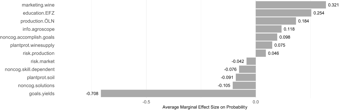
While descriptive results show notable differences between High- and Low-IPM-Adopters in our sample, not all differences are significant in predicting grower membership in either cluster. Results of the logit regression model give insights into the explanatory variables that are most predictive in determining cluster membership. More specifically, the model identifies which variables hold a statistically significant influence in predicting the adoption or non-adoption of High-IPM practices. Figure 4 shows the average marginal effect size (i.e., the percentage increase of being a High-IPM-Adopter upon a one-unit increase in the variable)Footnote 9 for the explanatory variables that were found to be statistically significant at the 5% level (for details see the Appendix, Section 4).
Significant predictors of High-IPM Cluster Membership.

The logit regression identifies a number of variables with a positive association with being a High-IPM-Adopter. Specifically, we find that farm and farmer characteristics such as marketing type (i.e., marketing mainly wines), the completion of an agricultural apprenticeship by the grape grower, and the production in accordance with cross-compliance is relevant. Additionally, the type of information on plant protection accessed by the grower matters, as we observe a positive effect of consulting federal research agencies (i.e., Agroscope). Results further indicate a significant positive association with selected behavioral factors, specifically non-cognitive skills, beliefs and risk attitudes. Specifically, the model predicts a higher likelihood of being a High-IPM-Adopter if growers are confident in their ability to achieve production goals, and if they believe that plant protection products positively impact wine supply. Notably, we find that the effect of risk aversion differs depending on the risk domain. While risk aversion in the production domain positively affects High-IPM adoption, risk aversion in the market domain has a negative effect.
V. Discussion
We analyze patterns of pesticide reduction measures in Swiss viticulture, focusing on their joint adoption as part of bundles. Specifically, we use a contingency analysis, a k-means algorithm, and a logit regression model to determine (i) which measures are frequently adopted as part of bundles and (ii) how bundle composition is shaped through farm and farmer characteristics, behavioral factors, and environmental influences.
Results indicate that labor and capital constraints play are relevant for the joint and separate adoption of individual measures. Specifically, we find that measures associated with a low capital- and labor-intensity (e.g., decision support tools, preventative measures, the promotion of beneficial insects) are more frequently adopted as bundles. Conversely, particularly capital- or labor-intense measures (e.g., sanitation, mechanical weeding) are generally adopted as stand-alone measures. This is intuitive, as viticulture is capital- and labor-demanding already without the adoption of additional measures (Schumacher et al., Reference Schumacher, Hirsch, Leumann and Wirthner2007) particularly in the plant protection domain (Chen et al., Reference Chen, Herrera, Benitez, Hoffmann, Möth, Paredes, Plaas, Popescu, Rascher, Rusch, Sandor, Tolle, Willemen, Winter and Schwarz2022), acting as a barrier to the joint adoption of particularly intensive measures. Additionally, results indicate that frequently bundled measures are characterized by low pesticide reduction potentials, indicating that a higher number of measures is needed to reduce pesticide use without compromising yields. Growers in our sample thus follow a bundled approach to pesticide substitution, as highlighted in related literature (see e.g., Finger et al., Reference Finger, Sok, Ahovi, Akter, Bremmer, Dachbrodt-Saaydeh, de Lauwere, Kreft, Kudsk, Lambarraa-Lehnhardt, McCallum, Lansink, Wauters and Möhring2024). Our findings further highlight the relevance of interdependencies between measures, with growers appearing to exploit complementary measures even when their joint use is associated with higher labor and capital demand. Specifically, growers in the sample make use of complementary effects between fungicide reduction (i.e., as a result of adopting fungus-resistant varieties) and the promotion of beneficial insects (see, e.g., Reiff et al., Reference Reiff, Sudarsan, Hoffmann and Entling2023). The adoption of both measures can be highly capital-intensive (see the Appendix, Section 1), but the complementarity between both measures appear to outweigh these financial drawbacks. However, as the use of fungus-resistant varieties is also associated with a reduction in labor demand (see, e.g., Pedneault and Provost, Reference Pedneault and Provost2016), this might also free up labor to be used for the adoption of additional measures. The interplay of capital, labor, and pesticide reduction potential is thus highly relevant for shaping pest management strategies, emphasizing the need for holistic perspectives beyond adoption behavior on a measure-level. Additional potential complementarities also remain to be explored, e.g., with regards to mechanical insect control and mechanical weeding.
The results of the cluster analysis indicate that the growers in our sample can be categorized into two groups of approximately equivalent size. Cluster 1 comprises 52% of the farms (n = 177), while Cluster 2 encompasses 48% (n = 164). Given that Cluster 2 farms adopt a range of pesticide reduction measures to a greater extent than Cluster 2, this cluster is described as “High-IPM-Adopters,” and Cluster 1 as “Low-IPM-Adopters,” with IPM principles as a benchmark (see Barzman et al., Reference Barzman, Bàrberi, Birch, Boonekamp, Dachbrodt-Saaydeh, Graf, Hommel, Jensen, Kiss, Kudsk, Lamichhane, Messéan, Moonen, Ratnadass, Ricci, Sarah and Sattin2015). We find that clusters are not spatially correlated. However, we find notable differences between the two clusters with regards to farm characteristics (e.g., farm size and income share) and farmer characteristics (e.g., education, tasks, information sources), behavioral factors (e.g., risk and time preferences, goals and outlook), and environmental influences (biggest negative yield influences, disease pressure levels). However, our results of the logit regression model show that not all differences are determining factors in shaping cluster membership.
We identify the statistically significant determinants for the adoption/non-adoption of highly IPM. We find that the marketing approach (i.e., marketing wine rather than unprocessed grapes) is the strongest positive determinant for membership in the High-IPM-Adoption cluster. This is in line with related literature, for instance with regards to fungus-resistant varieties (Finger et al., Reference Finger, Zachmann and McCallum2023), and emphasizes the need for incentives for pesticide reduction across the wine supply chain, also incorporating wineries and retailers (see also Möhring et al., Reference Möhring, Ingold, Kudsk, Martin-Laurent, Niggli, Siegrist, Studer, Walter and Finger2020a).
We further find that IPM in viticulture is not linked to higher education. Similarly, IPM is not limited to extensive production systems (e.g., as part of IP-Suisse programs).Footnote 10 The adoption of IPM and pesticide reduction measures is thus not necessarily dependent on the adoption of specific production systems, but rather dependent on factors relating to farm, farmer, and environment.
Results indicate that alongside structural and demographic characteristics, behavioral factors are crucial in explaining the adoption of High-IPM practices, which is in line with related literature (e.g., Dessart et al., Reference Dessart, Barreiro-Hurlé and Van Bavel2019). For example, the goals set by the farmer are relevant. Specifically, we find that a production-oriented approach—characterized by high grape yields as the main goal—decreases the likelihood of being a High-IPM-Adopter substantially. This highlights the role of farmer identity and self-perception in promoting conservation behavior (e.g., Lavoie and Wardropper, Reference Lavoie and Wardropper2021), and emphasizes the need for policy action in viticulture also beyond financial incentives such as direct payments or price markups. Shaping farmer identity and culture is challenging but shall be considered as part of effective and efficient policymaking towards sustainable agriculture (Möhring et al., Reference Möhring, Ingold, Kudsk, Martin-Laurent, Niggli, Siegrist, Studer, Walter and Finger2020a). Nudges may represent a promising opportunity in this context, but have shown heterogeneous success (Zachmann et al., Reference Zachmann, McCallum and Finger2023a).
We further find that farmer personality significantly affects adoption decision, particularly with regards to non-cognitive skills. Specifically, we find that growers who are confident in the success of their farming activities are more likely to be High-IPM-Adopters. Conversely, farmers with a strong internal locus of control, who belief that the success of farming operations is directly dependent on their skill exhibit a lower likelihood for being High-IPM-Adopters. The negative effect of an internal locus of control may be an indication of lack of knowledge or perceived skill surrounding integrated plant protection practices. Lack of knowledge and experience has been linked to lower adoption of new practices in agriculture in general (Bakker et al., Reference Bakker, Sok, Van Der Werf and Bianchi2021), but also specifically with regards to viticulture (e.g., Lucchi and Benelli, Reference Lucchi and Benelli2018). Additionally, our findings emphasize the importance of non-cognitive skills and personality for the adoption of conservation behavior in general (Wüpper et al., Reference Wüpper, Bukchin‐Peles, Just and Zilberman2023). This highlights the potential of information provision, trainings, or peer-to-peer workshops in promoting both the awareness of, as well as the skill perceptions surrounding pesticide reduction measures.
Our results further indicate a significant influence of risk preferences on High-IPM adoption, particularly in the production and market domain. Therein, risk aversion in the production domain is associated with a higher probability of being a High-IPM-Adopter, while the opposite is true for risk aversion in the market domain. These findings are in line with related literature. For example, Horowitz and Lichtenberg (Reference Horowitz and Lichtenberg1994) identify a risk-increasing effect of pesticides on production, meaning that growers exhibiting a stronger production risk aversion may be more likely to adopt a highly integrated plant protection approach with lower pesticide reliance. This is in line with literature relating a higher risk aversion to more intense pesticide usage (Fouillet et al., Reference Fouillet, Delière, Chartier, Munier-Jolain, Cortel, Rapidel and Merot2022). Conversely, literature identifies perceived market and institutional risks as significant adoption barriers to pesticide reduction (Garcia et al., Reference Garcia, Niklas, Wang and Finger2024a), which aligns with the negative effect of market risk aversion we identify as part of our analysis. Overall, these findings emphasize the need for the explicit consideration of risk preferences and risk perceptions, particularly under consideration of domain-specific preferences (Garcia et al., Reference Garcia, McCallum and Finger2024b), and their variations across production contexts.
Finally, we find that the type of information accessed by the farmer matters, as growers using information from federal research agencies such as Agroscope are more likely to be High-IPM-Adopters. This emphasizes the role of information sources for farmer conservation behavior (e.g., Wüpper et al., Reference Wüpper, Roleff and Finger2021), and underlines the relevance of information provision to promote sustainability transitions in viticulture and beyond.
VI. Conclusion
In light of our findings, we make the following recommendations for policy: (1) Our findings emphasize the role of measure bundles particularly in the context of pesticide reduction. Policy shall thus not only focus on the support of individual measures in isolation but also foster the adoption of effective and efficient bundles. (2) Action is needed across the grapevine value chain, also including wineries and retailers. This may be particularly effective in incentivizing growers marketing unprocessed grapes who are currently less likely to adopt a highly integrated approach to pest management. Measures could include price markups for grapes produced in low-pesticide production systems with more IPM approaches. (3) Information provision is crucial to move current Low-IPM-Adopters toward a more integrated approach, by removing adoption barriers related to the adoption of new and unfamiliar measures. Targeted information provision shall also aim to influence farmer self-perception, to incentivize a shift from a production-oriented perspective to a more conservational approach. This is crucial, as farmer self-identity and goals are significant determinants of their High-IPM adoption. The provision of information could entail the use of nudges, peer-to-peer learning, workshops, or trainings in a combined approach. (4) Risk preferences must be considered in the design of agricultural policies. For example, possible risk-reducing effects of pesticide reduction in the production domain could be communicated to farmers. Moreover, policy can contribute to reduce (perceived) risk with regards to markets and institutions to lower adoption barriers. This could include creating more stable policy environments and the provision of additional risk management tools.
Our analysis has implications for future research. Firstly, to better understand interdependencies and identify causal effects on promoters and barriers for the adoption of various pesticide reduction measures, further research is necessary. Moreover, further analysis on the realized reduction in pesticide applications and risks behind bundles of adoption, and further potential complementary effects between measures will contribute to a more nuanced and holistic understanding of farmer choices and the associated environmental impacts. Along these lines, additional assessments on differences between clusters could be improved by assessing details on production, pesticide use, risk, and environmental outcomes (e.g., biodiversity), which is currently limited by data constraints. Lastly, our analysis of combinations and clusters of pesticide reducing measures shall be also applied beyond viticulture and beyond Switzerland, thus contributing to sustainability transitions in agriculture as a whole.
Acknowledgements
We thank all farmers who participated in the survey. We thank the editor and reviewers for constructive feedback on earlier drafts of the paper. The study relied on financial support given by the ETH Foundation and Uniscientia Foundation within the project “Towards pesticide free agricultural production systems.”
Appendix
1. Assessment of available pesticide reduction strategies
In the following, we provide a detailed literature background for the assessment of each pesticide reduction measure that may be used by farmers in the sample, in accordance with the four main measure criteria: capital-intensity, labor-intensity, pesticide reduction potential, as well as involved time lag between measure implementation and realized measure effect.
1.1. Fungicide reduction measures
Sanitation
Sanitation is a lagged measure that entails the removal and pruning of infected plant material from the vineyard area, which significantly reduces the infection probability in the next growing season. As sanitation is typically done manually, it is characterized by a high labor-intensity. However, no additional capital is required, resulting in a low capital-intensity. While sanitation may be effective in controlling overwintering inoculum (Pertot et al., Reference Pertot, Caffi, Rossi, Mugnai, Hoffmann, Grando, Gary, Lafond, Duso, Thiery, Mazzoni and Anfora2017), it is commonly employed in combination with decision support tools (i.e., to schedule sanitation timepoints) and fungicides in the following growing season (Caffi et al., Reference Caffi, Legler, Bugiani and Rossi2013). The reduction potential is thus moderate.
Canopy management
Another lagged measure involving cluster thinning, shoot removal, or leaf removal early in the growing season, which may significantly reduce disease pressure at later points in time (Gubler, Reference Gubler1987). Canopy management practices may reduce yield losses from fungal diseases, but their use is not automatically associated with a reduction in fungicide use, as they are typically also an integral part of vine yield management in general (Mailly et al., Reference Mailly, Hossard, Barbier, Thiollet-Scholtus and Gary2017). Their reduction potential is thus characterized as moderate. As with sanitation, canopy management relies not on additional inputs but rather manual labor, resulting in a high labor-intensity and a low capital-intensity.
Decision support tools (fungicides and insecticides)
Decision support tools are used to optimize the timing and intensity of a pesticide application, e.g., in response to weather conditions favoring the development of a specific inoculum (see Fouillet et al., Reference Fouillet, Delière, Chartier, Munier-Jolain, Cortel, Rapidel and Merot2022). At the base of many decision support tools are disease models, that simulate the development of pathogens and diseases over time, and given the current environmental conditions. Decision support tools may significantly reduce the amount of pesticide used in comparison to routine applications of both fungicides (e.g., Gil et al., Reference Gil, Llorens, Landers, Llop and Giralt2011 ) and insecticides (Winkler et al., Reference Winkler, Bauer, Jung, Kleinhenz and Racca2024), resulting in a moderate overall reduction potential. As decision support tools are typically free and require little additional manual labor, both capital- and labor-intensity are characterized as low. Lastly, while decision support tool use forecasting systems, their effect is immediate, i.e., they reduce pesticide use without an associated time lag.
Microorganisms
Microorganisms (e.g., Bacillus subtilis) are parts of biopesticides which may be combined with other natural molecules to reduce the use of synthetic pesticides without a time lag, through antibiosis, induction of chemical resistance in the vine, parasitism of, or competition for nutrients with the pathogen (Pertot et al., Reference Pertot, Caffi, Rossi, Mugnai, Hoffmann, Grando, Gary, Lafond, Duso, Thiery, Mazzoni and Anfora2017). Microorganisms may significantly reduce disease pressure, but their efficacy may be reduced by varying environmental conditions (Altieri et al., Reference Altieri, Rossi and Fedele2023), thus resulting in a moderate reduction potential overall. Additionally, products containing microorganisms may also not always be commercially available on a large-scale (Pertot et al., Reference Pertot, Caffi, Rossi, Mugnai, Hoffmann, Grando, Gary, Lafond, Duso, Thiery, Mazzoni and Anfora2017), and thus likely more capital-intensive. Additionally, their reduced efficacy of biopesticides requires a higher number of applications, implying a moderate increase in labor-intensity.
Fertilizer Management
Fertilizer management involves the practice of applying nutrients to the vine foliage at the right times in order to prevent fungal disease spread (Calzarano et al., Reference Calzarano, Amalfitano, Seghetti and Di Marco2023). While their use has been observed to reduce pathogen incidence on the treated leaves, full effects are dependent on local conditions, resulting in a low reduction potential. Increases in fertilizer prices may also make this method more capital-intensive than synthetic pesticides. As with biopesticides, labor-intensity is higher than for synthetic fungicides (lower efficacy).
Inorganic Compounds
Inorganic compoundsFootnote 11 (e.g., Potassium bicarbonate) have an immediate control effect and are effective against fungal diseases (Laurent et al., Reference Laurent, Makowski, Aveline, Dupin and Miguez2021) but their efficacy as a stand-alone measure is low, implying a higher labor-intensity compared to synthetic fungicides. However, inorganic compounds are commonly less capital-intensive synthetic fungicides (Laurent et al., Reference Laurent, Makowski, Aveline, Dupin and Miguez2021).
Fungus-resistant varieties
Fungus-resistant grapevine varieties are characterized by higher resistance levels to common fungal pathogens (Pertot et al., Reference Pertot, Caffi, Rossi, Mugnai, Hoffmann, Grando, Gary, Lafond, Duso, Thiery, Mazzoni and Anfora2017), thus carrying the highest reduction potential for synthetic fungicides (Pedneault and Provost, Reference Pedneault and Provost2016). This also reduces the labor-intensity compared to synthetic fungicides, as fewer pesticide applications are necessary. Their adoption however involves replanting of vineyards, resulting in a high capital-intensity (Droz, Reference Droz2019). The time needed for newly panted vines to mature further implies a time lag.
1.2. Herbicide reduction measures
Mechanical weeding
Mechanical weeding is a measure with an immediate effect that may be used as an alternative to herbicides between and within vineyard rows (Fouillet et al., Reference Fouillet, Delière, Chartier, Munier-Jolain, Cortel, Rapidel and Merot2022). Mechanical weeding can be effective in controlling weeds, but the implements required, as well as the additional workload compared to synthetic herbicides (Jacquet et al., Reference Jacquet, Delame, Lozano-Vita, Reboud and Huyghe2019) imply a moderate increase in both capital- and labor-intensity.
Mulching
Mulching is an immediate measure that involves the spread of various materials (e.g., straw) between and within vineyard rows to suppress weed growth (Follak et al., Reference Follak, Kirchinger, Menger, Redl, Schmid, Heßdörfer, Lardschneider, Remmele, Riedle-Bauer, Rosner, Steinkellner, Winter and Rathbauer2024), which carries a moderate to high reduction potential for synthetic herbicides. Mulching requires additional labor and—depending on the availability of mulching materials and machinery—may also be associated with an increase in capital-intensity.
1.3. Insecticide reduction measures
Promotion of beneficial insects
The promotion of beneficial insects relies on the competition of beneficial arthropods with common insect pathogens (Pertot et al., Reference Pertot, Caffi, Rossi, Mugnai, Hoffmann, Grando, Gary, Lafond, Duso, Thiery, Mazzoni and Anfora2017). Beneficial insects have been shown to effectively control common insect pests, either as stand-alone organisms (e.g., Gomez-Llano et al., Reference Gomez-Llano, Khanal, Acevedo and Mansour2025) or as part of a general increase in local biodiversity levels (Reiff et al., Reference Reiff, Ehringer, Hoffmann and Entling2021). However, while significant control effects can occur, they are highly context dependent (Pertot et al., Reference Pertot, Caffi, Rossi, Mugnai, Hoffmann, Grando, Gary, Lafond, Duso, Thiery, Mazzoni and Anfora2017). The capital- and labor-intensity associated with the promotion of beneficial insects may additionally vary greatly depending on the promotion method (i.e., augmentation vs. dissemination) as well as the targeted insect pests. This measure is thus associated with a moderate capital- and labor-intensity increase, and a low reduction potential for insecticides.
Pheromones/confusion techniques
Pheromone-based pesticide reduction measures commonly involve the use of sex-pheromones, typically for mating disruption of common insect pests with an immediate effect (Fouillet et al., Reference Fouillet, Delière, Chartier, Munier-Jolain, Cortel, Rapidel and Merot2022). While the use of pheromones as confusion techniques to inhibit successful mating can be effective in controlling insect pests (e.g., Cocco et al., Reference Cocco, Lentini and Serra2024), their success is context dependent (Pertot et al., Reference Pertot, Caffi, Rossi, Mugnai, Hoffmann, Grando, Gary, Lafond, Duso, Thiery, Mazzoni and Anfora2017), resulting in a low reduction potential. As up to 1000 pheromone dispensers may have to be deployed per ha (Pertot et al., Reference Pertot, Caffi, Rossi, Mugnai, Hoffmann, Grando, Gary, Lafond, Duso, Thiery, Mazzoni and Anfora2017), their initial deployment may be moderately labor intensive. However, as dispensers are effective over long time periods, their overall labor-intensity compared to synthetic insecticide is low. Furthermore, as some pheromone-based methods are not widely commercially available or still in early developmental stages (Gut et al., Reference Gut, Adams, Miller, McGhee and Thomson2019), their use represents a moderate increase capital-intensity.
Mechanical nets and traps
Netting around the vineyard area can exclude insect pests with a very high efficacy (e.g., Leach et al., Reference Leach, Mariani, Centinari and Urban2023) but installing the nets is associated with a high capital-intensity. When successful, nets may however reduce the need for insecticide applications almost completely, thus lowering the labor-intensity slightly.
Preventative methods
Preventative methods are additional lagged measures that may be used before the start of the growing season to provide additional control effect against insect pests at later points in time (Fouillet et al., Reference Fouillet, Delière, Chartier, Munier-Jolain, Cortel, Rapidel and Merot2022; Mailly et al., Reference Mailly, Hossard, Barbier, Thiollet-Scholtus and Gary2017). There is a broad range of preventative methods available which may already be realized without significant increases in capital- and labor-intensity. However, due to the multitude of influences that may affect the efficacy of preventative methods as stand-alone measures, their overall reduction potential is low.
Non-chemical insecticides
Non-chemical insecticides may be used to control insect pests as an alternative to synthetic insecticides (Pertot et al., Reference Pertot, Caffi, Rossi, Mugnai, Hoffmann, Grando, Gary, Lafond, Duso, Thiery, Mazzoni and Anfora2017), but their efficacy is lower than for synthetic insecticides, thus increasing the labor-intensity. Their manufacturing may also be more capital-intensive than for synthetic insecticides.
1.4. Precision application technologies
When pesticides are applied using non-precision implements, run-off and drift may be significant (Otto et al., Reference Otto, Loddo, Baldoin and Zanin2015). Precision application technologies may be used to increase the application efficiency of all pesticide categories with immediate effect. All technologies are assumed to increase capital-intensity due to the associated investment costs, which are likely to outweigh costs savings for reduced pesticide quantities. Some technologies additionally imply an moderate to high increase in labor requirement.
2. Data
2.1. Overview and summary statistics
This study uses data which comprises 436 observations of Swiss grapevine growers and was collected in Spring 2022. The survey addressed farmers in all 6 winegrowing regions and in 3 languages (German, French, Italian), and the responding farms collectively encompass a vineyard area of 2'112.2, which constitutes 14.4% of the total cultivated grapevine area in Switzerland. Additional detail on the data is given in Zachmann, McCallum and Finger (Reference Zachmann, McCallum and Finger2023b).
2.2. Data preparation
We apply a two-step data preparation procedure to minimize biases and the influence of potential outliers. In a first step, organic farms are excluded from analysis as the uptake of organic practices does not allow for the use of certain plant protection practices. Additionally, the influence of outliers is minimized by using the interquartile range method. Thus, the final dataset used for analysis is reduced to 313 observations.
3. Details on the k-means analysis
3.1. Empirical basis
The k-means algorithm groups observations in the dataset by using  $k$ clusters, to which it repeatedly assigns centroids at random (Steinly, Reference Steinley and Brusco2011). The value of $k$ is determined using 23 estimation criteriaFootnote 12, and the $k$ to the highest number of estimation criteria is then used for further analysis. Once $k$ cluster centroids have been randomly assigned, the following formula is used to calculate each data point's Euclidian distance from the initial centroids:
 \begin{equation}\text{Distance}(x_i, c_k) = \sqrt{\sum_{d=1}^{D} (x_{id} - c_{kd})^2} ,\end{equation}
where  ${x_i}$ represents a datapoint (i.e., a farm) and ${c_k}$ the centroids for all pre-determined clusters $k$.
$k$.  $D$ represents the number of dimensions in the data (i.e., the number of assessed strategies. Using Equation (1), each datapoint is assigned to the centroid which it is closest to. The algorithm then reassesses the value of the cluster centroids using:
 \begin{equation}c_i = \frac{1}{n_k} \sum_{i=1}^{n_k} x_k,\end{equation}
where  ${n_k}$ is the number of datapoints in each cluster $k$, and ${x_k}$ represents all the datapoints $x$ that were assigned to each $k$. The new centroid value ${c_i}$ is calculated using the means of all datapoints assigned to it. With Equation (1), the distance of all datapoints to the new centroids is calculated again, and datapoints are re-assigned to their closest centroid. Equation (2) is then used once more to re-calculate centroid values and repeated until the centroids in each cluster no longer shift significantly after using Equation (2). Objectively, this can be expressed as
 \begin{equation}
J = \sum_{j=1}^k \left( \sum_{x_i \in C_j} (x_i - c_j)^2 \right)\end{equation}
\begin{equation}
J = \sum_{j=1}^k \left( \sum_{x_i \in C_j} (x_i - c_j)^2 \right)\end{equation}where  $J$ represents the total within-cluster variation (i.e., the sum of squared distances between each datapoint and its assigned cluster centroid. The k-means algorithm minimizes $J$ so that each centroid's cluster of datapoints is as tight as possible. Equation (1) and (2) are repeated until the change in $J$ with each iteration of the algorithm becomes negligible.
3.2. Outputs and index values
Table A1. gives an overview of the optimal number of clusters suggested by index, as well as the corresponding index values.
Overview of indices used for the k-means clustering algorithm

4. Result Details
4.1. Results of the k-means clustering analysis
Table A2. compares the average variable values across the whole dataset with averages for both clusters identified in the k-means analysis.
Comparison of variable means between Clusters 1 and 2

Red indicates negative and blue positive deviations from the data average within the clusters.
4.2. Spatial correlation of clusters—regional
To determine whether the observed differences in measure bundle adoption between the two clusters are behavioral rather than spatial, we perform a series of tests. First, we aggregate clusters by region to identify which wine production region is more likely to belong to Cluster 1 than Cluster 2 and vice versa. Results indicate that the majority of wine producing regions (i.e., Deutschschweiz, Geneve, Valais, and Vaud) are approximately equally divided between Cluster 1 and Cluster 2. Disparities in membership are evident only for Ticino and Trois lacs, which appear to belong predominantly to Cluster 1, indicating a higher propensity to adopt Low-IPM strategies in these regions. To determine if differences in cluster membership across regions occur due to spatial autocorrelation, we use a weight matrix. The output of the Moran's I statistic (Figure A1) reads:
Moran’s I output for regional autocorrelation.

The spatial autocorrelation observed in the survey data (−0.24) is close to the expected autocorrelation under complete randomness (−0.2), indicating that there is no spatial autocorrelation of clusters in the analyzed sample. Thus, while some regions are much more likely to belong to one cluster over the other, this effect is not observed between neighboring regions, i.e., there is no spatial component to cluster membership. The p-value of 0.57 confirms these findings. We thus conclude that the clustering observed in the k-means analysis is a result of behavioral and structural nature rather than spatial.
4.3. Spatial correlation of clusters—cantonal
As wine regions in the sample are vast (see https://www.myswitzerland.com/de-ch/erlebnisse/sommer-herbst/oenotourismus/schweizer-wein/ for reference), we also test for spatial correlation on a cantonal, i.e., smaller-scale level. Results of cluster membership per canton as well as the results of the Moran’s I statistic are indicated below (Figure A2).

We find that cluster membership varies between cantons. However, this variation does not seem to be related to a canton’s neighbors, as evidenced by the Moran’s statistic of our spatial weight matrix (Figure A2). The autocorrelation in our sample is 0.38 (compared to −0.05 under complete randomness) and the p-value is 0.27, indicating that there is no spatial autocorrelation on a cantonal level in the analyzed sample. We thus conclude that the observed differences between clusters are indeed of behavioral and structural nature.
4.4. Results of the logit model
The regression used for the logit analysis can be expressed as:
 \begin{equation*}\log \left( {\frac{{{p_i}}}{{1 - {p_i}}}} \right) = {\beta _0} + {\beta _1}{\text{Va}}{{\text{r}}_1} + \ldots + {\beta _k}{\text{Va}}{{\text{r}}_k},\end{equation*}
where  ${p_i}$ denotes the probability of farmer membership in the High-IPM cluster, conditional on the explanatory variables ${\text{Var}}$. ${\beta _0}$, ${\beta _1}$, and ${\beta _k}$ denote the coefficient estimates for each of these variables. For additional information on variable coding and description, please refer to Zachmann et al. (Reference Zachmann, McCallum and Finger2023b).
Table A3. shows the average marginal effect size (AME) for the explanatory variables that were found to be statistically significant at least at the 5% level. It also gives an indication on the average effect size, the standard error, as well as associated z-values.
Average marginal effect size for significant explanatory variables

Legend:
marketing.wine = grower sells mainly wine
education.EFZ = grower has completed an agricultural apprenticeship as the highest degree
production.ÖLN = production in accordance with ecological cross compliance
info.agroscope = federal research agencies (i.e., Agroscope) are consulted for information on plant protction
noncog.accomplish.goals = belief that production goals will be accomplished at harvest
plantprot.winesupply = belief that plant protection products have a positive impact on wine supply
risk.production = risk aversion in the production domain
risk.market = risk aversion in the market domain
noncog.skill.dependent = belief that production success is dependent on grower's own skill
plantprot.soil = belief that plant protection products have a positive impact on soil health
goals.yields = high yields are the most important goal


 Open access