


1. Introduction
Bubble-laden turbulent flows are prevalent in both environmental and industrial scenes. In nature, bubbles play important roles, such as air bubbles at the ocean–atmosphere interface and the absorption of greenhouse gases (Thorpe Reference Thorpe1982; Zappa, Asher & Jessup Reference Zappa, Asher and Jessup2001). In industrial applications, bubble-laden flows are commonly encountered in bubble columns used in chemical reactors and cavitation within the hydraulic machinery (Arndt Reference Arndt1981; Kantarci, Borak & Ulgen Reference Kantarci, Borak and Ulgen2005). The bubble also exhibits significant potential for turbulent drag reduction, which is environmentally friendly and easy to implement (Mccormick & Bhattacharyya Reference Mccormick and Bhattacharyya1973). In most of these scenarios, bubbles demonstrate complex dispersion behaviours and interact intricately with turbulent flow structures.
Due to their low-density ratio, $\varGamma =\rho _b/\rho _f\ll 1$
, where
$\varGamma =\rho _b/\rho _f\ll 1$
, where $\rho _b$
and
$\rho _b$
and $\rho _f$
denote the densities of bubble and liquid phases, respectively, the dynamics of bubbles in turbulent flows differ from those of heavy or neutrally buoyant particles. There are several important dimensionless numbers governing the bubble behaviours: the Stokes number,
$\rho _f$
denote the densities of bubble and liquid phases, respectively, the dynamics of bubbles in turbulent flows differ from those of heavy or neutrally buoyant particles. There are several important dimensionless numbers governing the bubble behaviours: the Stokes number, $St=\tau _b/\tau _f$
, which represents the ratio of bubble response time
$St=\tau _b/\tau _f$
, which represents the ratio of bubble response time $\tau _b$
and the characteristic fluid time scale
$\tau _b$
and the characteristic fluid time scale $\tau _f$
; the Froude number,
$\tau _f$
; the Froude number, $\textit{Fr}=a_f/a_b$
, which quantifies the ratio of characteristic fluid acceleration
$\textit{Fr}=a_f/a_b$
, which quantifies the ratio of characteristic fluid acceleration $a_f$
and bubble acceleration due to buoyancy
$a_f$
and bubble acceleration due to buoyancy $a_b$
; and the Eötvös number,
$a_b$
; and the Eötvös number, $Eo=gd^2 (\rho _f-\rho _b )/\sigma$
, which compares the effects of buoyancy and capillary forces, where
$Eo=gd^2 (\rho _f-\rho _b )/\sigma$
, which compares the effects of buoyancy and capillary forces, where $\sigma$
denotes the surface tension (Mathai, Lohse & Sun Reference Mathai, Lohse and Sun2020).
$\sigma$
denotes the surface tension (Mathai, Lohse & Sun Reference Mathai, Lohse and Sun2020).
Bubble size plays a crucial role in determining bubble dynamics, as quantified by the Stokes number $St$
. Very small bubbles with low
$St$
. Very small bubbles with low $St$
respond almost instantaneously to flow fluctuations, making them effective fluid tracers for flow visualisation (Lu & Smith Reference Lu and Smith1985). Druzhinin & Elghobashi (Reference Druzhinin and Elghobashi1998) studied microbubbles in homogeneous isotropic turbulence and observed minimal preferential concentration due to their small
$St$
respond almost instantaneously to flow fluctuations, making them effective fluid tracers for flow visualisation (Lu & Smith Reference Lu and Smith1985). Druzhinin & Elghobashi (Reference Druzhinin and Elghobashi1998) studied microbubbles in homogeneous isotropic turbulence and observed minimal preferential concentration due to their small $St$
. As
$St$
. As $St$
increases (
$St$
increases ( $St\lt 1$
), bubbles exhibit stronger preferential concentration, scaling approximately linearly with
$St\lt 1$
), bubbles exhibit stronger preferential concentration, scaling approximately linearly with $St$
(Balachandar & Eaton Reference Balachandar and Eaton2010). The strongest clustering in homogeneous isotropic turbulence occurs at
$St$
(Balachandar & Eaton Reference Balachandar and Eaton2010). The strongest clustering in homogeneous isotropic turbulence occurs at $St\approx 1$
, indicating substantial coupling with the smallest Kolmogorov scale (Wang & Maxey Reference Wang and Maxey1993; Tagawa et al. Reference Tagawa, Mercado, Prakash, Calzavarini, Sun and Lohse2012). Bubbles with moderate
$St\approx 1$
, indicating substantial coupling with the smallest Kolmogorov scale (Wang & Maxey Reference Wang and Maxey1993; Tagawa et al. Reference Tagawa, Mercado, Prakash, Calzavarini, Sun and Lohse2012). Bubbles with moderate $St$
tend to be trapped within vortices due to the centripetal action of inertial forces, accumulating in regions of high enstrophy and low pressure (Ruetsch & Meiburg Reference Ruetsch and Meiburg1993; Maxey, Chang & Wang Reference Maxey, Chang and Wang1994).
$St$
tend to be trapped within vortices due to the centripetal action of inertial forces, accumulating in regions of high enstrophy and low pressure (Ruetsch & Meiburg Reference Ruetsch and Meiburg1993; Maxey, Chang & Wang Reference Maxey, Chang and Wang1994).
Gravity also has a significant influence on bubble dynamics, as characterised by the Froude number $\textit{Fr}$
. At low
$\textit{Fr}$
. At low $\textit{Fr}$
(
$\textit{Fr}$
( $\textit{Fr}\lt 1$
), buoyancy force induces a non-negligible mean slip velocity along the gravitation direction, leading to crossing-trajectory behaviours (Mathai et al. Reference Mathai, Lohse and Sun2020). Sene, Hunt & Thomas (Reference Sene, Hunt and Thomas1994) noted that bubbles tend to be trapped within vortices only when the characteristic vortex velocity exceeds the slip velocity. Mathai et al. (Reference Mathai, Calzavarini, Brons, Sun and Lohse2016) found that gravity amplifies acceleration variance even for bubbles with
$\textit{Fr}\lt 1$
), buoyancy force induces a non-negligible mean slip velocity along the gravitation direction, leading to crossing-trajectory behaviours (Mathai et al. Reference Mathai, Lohse and Sun2020). Sene, Hunt & Thomas (Reference Sene, Hunt and Thomas1994) noted that bubbles tend to be trapped within vortices only when the characteristic vortex velocity exceeds the slip velocity. Mathai et al. (Reference Mathai, Calzavarini, Brons, Sun and Lohse2016) found that gravity amplifies acceleration variance even for bubbles with $St\ll 1$
, leading to suppression of the decorrelation time with fluid. They emphasised that microbubbles may not serve as faithful tracers unless
$St\ll 1$
, leading to suppression of the decorrelation time with fluid. They emphasised that microbubbles may not serve as faithful tracers unless $St/Fr\ll 1$
. The buoyancy-induced slip also introduces a lift force perpendicular to the slip. Mazzitelli et al. (Reference Mazzitelli, Lohse and Toschi2003b
) pointed out that lift force pushes bubbles to the downward side of the vortex, preventing them from approaching the centres of vortices. Bubble deformability, quantified by the Eötvös number,
$St/Fr\ll 1$
. The buoyancy-induced slip also introduces a lift force perpendicular to the slip. Mazzitelli et al. (Reference Mazzitelli, Lohse and Toschi2003b
) pointed out that lift force pushes bubbles to the downward side of the vortex, preventing them from approaching the centres of vortices. Bubble deformability, quantified by the Eötvös number, $Eo$
, also strongly affects the bubble motion and concentration. This is primarily because the drag force and lift force acting on the bubbles are shape-dependent (Ni Reference Ni2024). Notably, the lift force is highly sensitive to bubble deformation, as its direction is gradually reversed as deformation increases (Tomiyama et al. Reference Tomiyama, Tamai, Zun and Hosokawa2002; Atasi et al. Reference Atasi, Ravisankar, Legendre and Zenit2023).
$Eo$
, also strongly affects the bubble motion and concentration. This is primarily because the drag force and lift force acting on the bubbles are shape-dependent (Ni Reference Ni2024). Notably, the lift force is highly sensitive to bubble deformation, as its direction is gradually reversed as deformation increases (Tomiyama et al. Reference Tomiyama, Tamai, Zun and Hosokawa2002; Atasi et al. Reference Atasi, Ravisankar, Legendre and Zenit2023).
The preferential concentration of bubbles in wall-bounded turbulent flows introduces additional complexities. In upflows, gravity acts opposite to the flow direction, imparting a positive streamwise slip velocity and a lift force that pushes the bubble towards the wall; in downflows, the opposite occurs (Kashinsky & Randin Reference Kashinsky and Randin1999; Hibiki et al. Reference Hibiki, Goda, Kim, Ishii and Uhle2004). Giusti, Lucci & Soldati (Reference Giusti, Lucci and Soldati2005) pointed out that in the upflow (downflow), the lift force displaces bubbles away from (towards) the quasi-streamwise vortices, resulting in preferential concentration in low-speed (high-speed) regions. Park et al. (Reference Park, Saito, Tasaka and Murai2019) conducted experiments in the horizontal turbulent boundary layer and found that microbubbles accumulate within low-speed streaks in the viscous sublayer and hairpin vortices in the buffer layer. Similar wall-accumulation and preferential concentration in low-speed streaks are commonly observed in inertial particle-laden flows and are attributed to the well-known turbophoresis mechanism (Caporaloni et al. Reference Caporaloni, Tampieri, Trombetti and Vittori1975; Narayanan et al. Reference Narayanan, Lakehal, Botto and Soldati2003). Turbophoresis drives inertia particles towards the wall, requiring particles to persist in low-speed ejection regions to balance the turbophoretic fluxes (Picano, Sardina & Casciola Reference Picano, Sardina and Casciola2009). Turbophoresis is most effective for particles with moderate inertia $(St=10\sim 50)$
, whose response time scales match those of near-wall vortices (Sardina et al. Reference Sardina, Picano, Schlatter, Brandt and Casciola2011). However, due to the small
$(St=10\sim 50)$
, whose response time scales match those of near-wall vortices (Sardina et al. Reference Sardina, Picano, Schlatter, Brandt and Casciola2011). However, due to the small $St$
in bubble-laden flow, the effect of turbophoresis on bubbles is limited, while it inspires us to investigate the roles of the wall-normal forces on preferential concentration.
$St$
in bubble-laden flow, the effect of turbophoresis on bubbles is limited, while it inspires us to investigate the roles of the wall-normal forces on preferential concentration.
Bubbles in wall-bounded flows also interact dynamically with turbulence. Their presence directly modifies local fluid properties, such as density and viscosity (Legner Reference Legner1984). Kanai & Miyata (Reference Kanai and Miyata2001) found that bubbles prevent the formation of spanwise vortices and suppress bursting events. Ferrante & Elghobashi (Reference Ferrante and Elghobashi2004) observed that bubbles induce positive local fluid velocity divergence, generating positive wall-normal velocities that displace the quasi-streamwise vortices away from the wall. Ortiz-Villafuerte & Hassan (Reference Ortiz-Villafuerte and Hassan2006) emphasised that the local void fraction in the buffer layer significantly affects drag reduction, indicating dynamic bubble interaction with turbulent structures in the buffer layer. Jacob et al. (Reference Jacob, Olivieri, Miozzi, Campana and Piva2010) showed that the coherence of near-wall structures is decreased by the bubble feedback force. Lu, Fernández & Tryggvason (Reference Lu, Fernández and Tryggvason2005) highlighted the roles of bubble deformation and breakup in turbulence modulation, while these effects can be neglected for small bubbles. The bubble size is also an important factor for turbulence modulation (Murai, Qu & Yamamoto Reference Murai, Qu and Yamamoto2006). Kato et al. (Reference Kato, Iwashina, Miyanaga and Yamaguchi1999) stressed that large bubbles enhance turbulence, whereas small bubbles suppress it, which is similar to solid particles. Verschoof et al. (Reference Verschoof, van der Veen, Sun and Lohse2016) showed that large and deformable bubbles near the wall partially block the outward transportation of coherent structures and pointed out that bubble drag reduction requires large bubbles.
With the development of computational capability, numerical studies on bubble-laden flows have grown rapidly over the past two decades, introducing a range of numerical methods. The Euler–Euler (E–E) method treats the dispersed phase as a fluid media and models the interface transfer, which is suitable for dense two-phase flows (Druzhinin & Elghobashi Reference Druzhinin and Elghobashi1998; Haji Mohammadi et al. Reference Haji Mohammadi, Sotiropoulos and Brinkerhoff2019). In contrast, the interface-resolving method fully captures the bubble–fluid interface and is typically used for large bubbles ( $d\gt \eta$
) (Bunner & Tryggvason Reference Bunner and Tryggvason2003; Lu & Tryggvason Reference Lu and Tryggvason2013). However, this method is computationally expensive and limited to small bubble counts. The Euler–Lagrange (E–L) method treats bubbles as point particles and tracks their trajectories individually, combining the advantages of these two methods (Maxey & Riley Reference Maxey and Riley1983; Wang & Maxey Reference Wang and Maxey1993). Xu et al. (Reference Xu, Maxey and Karniadakis2002) conducted the earliest Euler–Lagrange study of bubble-laden wall-bounded turbulent flow, with direct numerical simulation (DNS) for the fluid phase. This method has been proven successful in studies of turbulent boundary layer (Mattson & Mahesh Reference Mattson and Mahesh2011; Zhang, Wang & Wan Reference Zhang, Wang and Wan2020) and channel flow (Pang, Wei & Yu Reference Pang, Wei and Yu2010; Molin, Marchioli & Soldati Reference Molin, Marchioli and Soldati2012). Breuer & Hoppe (Reference Breuer and Hoppe2017) coupled large eddy simulation (LES) with the E–L method, incorporating a Langevin model for the subgrid-scale effect. When bubble volume fraction is low enough (
$d\gt \eta$
) (Bunner & Tryggvason Reference Bunner and Tryggvason2003; Lu & Tryggvason Reference Lu and Tryggvason2013). However, this method is computationally expensive and limited to small bubble counts. The Euler–Lagrange (E–L) method treats bubbles as point particles and tracks their trajectories individually, combining the advantages of these two methods (Maxey & Riley Reference Maxey and Riley1983; Wang & Maxey Reference Wang and Maxey1993). Xu et al. (Reference Xu, Maxey and Karniadakis2002) conducted the earliest Euler–Lagrange study of bubble-laden wall-bounded turbulent flow, with direct numerical simulation (DNS) for the fluid phase. This method has been proven successful in studies of turbulent boundary layer (Mattson & Mahesh Reference Mattson and Mahesh2011; Zhang, Wang & Wan Reference Zhang, Wang and Wan2020) and channel flow (Pang, Wei & Yu Reference Pang, Wei and Yu2010; Molin, Marchioli & Soldati Reference Molin, Marchioli and Soldati2012). Breuer & Hoppe (Reference Breuer and Hoppe2017) coupled large eddy simulation (LES) with the E–L method, incorporating a Langevin model for the subgrid-scale effect. When bubble volume fraction is low enough ( $\alpha _v\lt 10^{-3}$
), the two-phase system can be regarded as a dilute suspension, where only the two-way coupling between bubbles and fluid needs to be considered (Elghobashi Reference Elghobashi1991, Reference Elghobashi1994). At higher volume fraction, the system transitions into a dense suspension, where the bubble–bubble interactions, including collision, breakup and coalescence, become significant, necessitating a four-way coupling (Asiagbe et al. Reference Asiagbe, Colombo, Fairweather and Njobuenwu2020; Zhai, Fairweather & Colombo Reference Zhai, Fairweather and Colombo2020). Additionally, in the two-way coupling simulations, the feedback force exerted by the bubbles perturbs the local flow field, thereby introducing errors in the calculation of the hydrodynamic forces. Consequently, an additional correction is necessary for finite-size bubbles (Balachandar & Liu Reference Balachandar and Liu2023). Most existing correction methods account only for the fluid velocity (Ireland & Desjardins Reference Ireland and Desjardins2017; Pakseresht, Esmaily & Apte Reference Pakseresht, Esmaily and Apte2020). Motta, Battista & Gualtieri (Reference Motta, Battista and Gualtieri2020) employed the exact regularised point particle method (ERPP) (Gualtieri et al. Reference Gualtieri, Picano, Sardina and Casciola2015) for the two-way coupling bubble-laden shear flow. Le Roy De Bonneville et al. (Reference Le Roy De Bonneville, Zamansky, Risso, Boulin and Haquet2021) proposed a comprehensive method that corrects not only the flow velocity, but also the spatial gradient and temporal derivative of flow velocity.
$\alpha _v\lt 10^{-3}$
), the two-phase system can be regarded as a dilute suspension, where only the two-way coupling between bubbles and fluid needs to be considered (Elghobashi Reference Elghobashi1991, Reference Elghobashi1994). At higher volume fraction, the system transitions into a dense suspension, where the bubble–bubble interactions, including collision, breakup and coalescence, become significant, necessitating a four-way coupling (Asiagbe et al. Reference Asiagbe, Colombo, Fairweather and Njobuenwu2020; Zhai, Fairweather & Colombo Reference Zhai, Fairweather and Colombo2020). Additionally, in the two-way coupling simulations, the feedback force exerted by the bubbles perturbs the local flow field, thereby introducing errors in the calculation of the hydrodynamic forces. Consequently, an additional correction is necessary for finite-size bubbles (Balachandar & Liu Reference Balachandar and Liu2023). Most existing correction methods account only for the fluid velocity (Ireland & Desjardins Reference Ireland and Desjardins2017; Pakseresht, Esmaily & Apte Reference Pakseresht, Esmaily and Apte2020). Motta, Battista & Gualtieri (Reference Motta, Battista and Gualtieri2020) employed the exact regularised point particle method (ERPP) (Gualtieri et al. Reference Gualtieri, Picano, Sardina and Casciola2015) for the two-way coupling bubble-laden shear flow. Le Roy De Bonneville et al. (Reference Le Roy De Bonneville, Zamansky, Risso, Boulin and Haquet2021) proposed a comprehensive method that corrects not only the flow velocity, but also the spatial gradient and temporal derivative of flow velocity.
In vertical turbulent channel flow, bubbles exhibit significant wall accumulation and preferential concentration behaviours (Giusti et al. Reference Giusti, Lucci and Soldati2005; Molin et al. Reference Molin, Marchioli and Soldati2012), yet the underlying mechanisms remain unclear. The preferential concentration mechanism of bubbles differs from that of inertial particles. For instance, inertial particles tend to accumulate in low-speed streaky structures (Soldati & Marchioli Reference Soldati and Marchioli2009), while preferential accumulation in high-speed regions has been observed in downward bubble-laden flows (Giusti et al. Reference Giusti, Lucci and Soldati2005). However, most existing studies on bubble-laden flows have focused on finite-size, deformable bubbles with moderate $St$
and large
$St$
and large $Eo$
, which exhibit strong two-way coupling with turbulent structures (García-Magariño et al. Reference García-Magariño, Lopez-Gavilan, Sor and Terroba2023). In contrast, studies on micro-size bubbles under the strong influence of gravity are relatively scarce (Mazzitelli et al. Reference Mazzitelli, Lohse and Toschi2003a
; Molin et al. Reference Molin, Marchioli and Soldati2012). The present study aims to investigate the dynamic characteristics of micro-size bubbles (
$Eo$
, which exhibit strong two-way coupling with turbulent structures (García-Magariño et al. Reference García-Magariño, Lopez-Gavilan, Sor and Terroba2023). In contrast, studies on micro-size bubbles under the strong influence of gravity are relatively scarce (Mazzitelli et al. Reference Mazzitelli, Lohse and Toschi2003a
; Molin et al. Reference Molin, Marchioli and Soldati2012). The present study aims to investigate the dynamic characteristics of micro-size bubbles ( $d/\eta \lt 1$
,
$d/\eta \lt 1$
, $St\ll 1$
,
$St\ll 1$
, $St/Fr\sim O ( 1 )$
and
$St/Fr\sim O ( 1 )$
and $Eo\ll 1$
) in the upward vertical channel using the E–L method. We primarily focus on the phenomena and the underlying mechanisms of bubble preferential concentration. We also analyse the flow field modification induced by bubbles. The remainder of this paper is structured as follows. The details of the numerical simulation are provided in § 2. Then, instantaneous and statistical results are presented and discussed in § 3. Finally, conclusions are drawn in § 4.
$Eo\ll 1$
) in the upward vertical channel using the E–L method. We primarily focus on the phenomena and the underlying mechanisms of bubble preferential concentration. We also analyse the flow field modification induced by bubbles. The remainder of this paper is structured as follows. The details of the numerical simulation are provided in § 2. Then, instantaneous and statistical results are presented and discussed in § 3. Finally, conclusions are drawn in § 4.
2. Problem formulation and numerical method
In this section, the numerical method employed for simulating bubble-laden turbulent channel flows is presented. A two-way coupling E–L method based on DNS is employed. The Eulerian phase represents slightly contaminated water with a density of $\rho _f=1\times 10^3\, \textrm{kg m}^{-3}$
and a kinematic viscosity of
$\rho _f=1\times 10^3\, \textrm{kg m}^{-3}$
and a kinematic viscosity of $\nu =1\times 10^{-6}\,\rm m^2\,s^{-1}$
. The Lagrangian phase represents air bubbles with a density of
$\nu =1\times 10^{-6}\,\rm m^2\,s^{-1}$
. The Lagrangian phase represents air bubbles with a density of $\rho _b=1.3\, \textrm{kg m}^{-3}$
and a surface tension coefficient of
$\rho _b=1.3\, \textrm{kg m}^{-3}$
and a surface tension coefficient of $\sigma =0.0728\rm \,N\,m^{-1}$
.
$\sigma =0.0728\rm \,N\,m^{-1}$
.
2.1. Governing equations
2.1.1. Eulerian fluid phase
The flow field is solved within the Eulerian framework, which is considered incompressible and adiabatic. The governing equations of the fluid phase are the continuity equation and the Navier–Stokes equation in the incompressible form:
 \begin{align} \frac {\partial u_i}{\partial x_i}&=0 , \end{align}
 \begin{align} \frac {\partial u_i}{\partial t}+u_j\frac {\partial u_i}{\partial x_j}&=-\frac {1}{\rho _f}\frac {\partial p}{\partial x_i}+\nu \frac {\partial ^2u_i}{\partial x_j\partial x_j}+\frac {1}{\rho _f}\frac {{\textrm{d}}P_0}{{\textrm{d}}x}\delta _{1,i}+\frac {f_i}{\rho _f} , \end{align}
where $u_i$
is the
$u_i$
is the $i{\textrm{th}}$
component of velocity,
$i{\textrm{th}}$
component of velocity, $p$
is pressure and
$p$
is pressure and $f_i$
is the feedback force from the bubbles to the flow. Here,
$f_i$
is the feedback force from the bubbles to the flow. Here, ${\textrm{d}}P_0/{\textrm{d}}x$
is the mean pressure gradient driving the flow, corresponding to a friction Reynolds number of
${\textrm{d}}P_0/{\textrm{d}}x$
is the mean pressure gradient driving the flow, corresponding to a friction Reynolds number of $Re_{\tau 0}=u_{\tau 0}h/\nu$
, where
$Re_{\tau 0}=u_{\tau 0}h/\nu$
, where $h$
is the channel half-width and
$h$
is the channel half-width and $u_{\tau 0}$
is the friction velocity of unladen flow,
$u_{\tau 0}$
is the friction velocity of unladen flow,
 \begin{align} u_{\tau 0}=\sqrt {\frac {{\textrm{d}}P_0}{{\textrm{d}}x}\frac {h}{\rho _f}} . \end{align}
In the upward vertical channel, gravity acts in the direction opposite to the flow. Bubbles experience a positive buoyancy force, which further contributes to an increase in both the fluid bulk velocity and wall shear stress. The actual friction velocity in the bubble-laden flow is (Molin et al. Reference Molin, Marchioli and Soldati2012)
 \begin{align} u_{\tau }=\sqrt {\frac {{\textrm{d}}P_0}{{\textrm{d}}x}\frac {h}{\rho _f}+\frac {\alpha _v(\rho _f-\rho _b)gh}{\rho _f}}. \end{align}
The corresponding friction Reynolds number for bubble-laden flow is $Re_{\tau }=u_{\tau }h/\nu$
. In this article, the superscript ‘
$Re_{\tau }=u_{\tau }h/\nu$
. In this article, the superscript ‘ $+0$
’ refers to normalisation using the unladen friction velocity
$+0$
’ refers to normalisation using the unladen friction velocity $u_{\tau 0}$
, while the superscript ‘
$u_{\tau 0}$
, while the superscript ‘ $+$
’ represents the normalisation using the actual friction velocity
$+$
’ represents the normalisation using the actual friction velocity $u_{\tau }$
.
$u_{\tau }$
.
2.1.2. Lagrangian bubble phase
The bubbles are assumed to be rigid spheres due to their small diameter and the presence of surface surfactants in the water. The surfactants accumulate on the bubble surface, leading to an assumption that the bubble surface approximates a no-slip boundary condition, thus neglecting internal circulation within the bubble (Ferrante & Elghobashi Reference Ferrante and Elghobashi2004).
The motion of bubbles in the flow is governed by Newton’s second law. Since the bubble density is significantly lower than the fluid $(\rho _b\ll \rho _f)$
, the forces acting on the bubbles must include the gravity force, buoyancy force, drag force, lift force, wall-lift force, pressure-gradient force, added mass force and Basset force. The Lagrangian motion equation can be written as (Maxey & Riley Reference Maxey and Riley1983)
$(\rho _b\ll \rho _f)$
, the forces acting on the bubbles must include the gravity force, buoyancy force, drag force, lift force, wall-lift force, pressure-gradient force, added mass force and Basset force. The Lagrangian motion equation can be written as (Maxey & Riley Reference Maxey and Riley1983)
 \begin{align} \dfrac {{\textrm{d}}\boldsymbol{x_b}}{{\textrm{d}}t}&=\boldsymbol{u}_b, \end{align}
 \begin{align} \dfrac {{\textrm{d}}\boldsymbol{u}_b}{{\textrm{d}}t} &=\underbrace {\left (1-\dfrac {\rho _f}{\rho _b}\right )\boldsymbol{g}}_{{\boldsymbol{F}_G}} +\underbrace {C_D\dfrac 3{4d}\dfrac {\rho _f}{\rho _b}|\boldsymbol{u}_s|\left (-\boldsymbol{u}_s\right )}_{{\boldsymbol{F}_D}} +\underbrace {C_L\dfrac {\rho _f}{\rho _b}\left (-\boldsymbol{u}_s\right )\times \left (\boldsymbol{\nabla }\times \boldsymbol{u}\right )_{@b}}_{{\boldsymbol{F}_L}} \nonumber \\ & +\underbrace {C_W\dfrac {\rho _f}{\rho _b}\dfrac 2d|u_{sw}|^2\hat {\boldsymbol{e}}_y}_{{\boldsymbol{F}_W}} +\underbrace {\dfrac {\rho _f}{\rho _b}\dfrac {{\textrm{D}}\boldsymbol{u}_{@b}}{{\textrm{D}}t}}_{{\boldsymbol{F}_P}} +\underbrace {C_M\dfrac {\rho _f}{\rho _b}\left (\dfrac {{\textrm{D}}\boldsymbol{u}_{@b}}{{\textrm{D}}t}-\dfrac {{\textrm{d}}\boldsymbol{u}_b}{{\textrm{d}}t}\right )}_{{\boldsymbol{F}_A}} \nonumber \\ & +\underbrace {C_B\int _{-\infty }^tK_B(t-\tau )\left (\dfrac {{\textrm{d}}\boldsymbol{u}_{@b}}{{\textrm{d}}t}-\dfrac {{\textrm{d}}\boldsymbol{u}_b}{{\textrm{d}}t}\right ){\textrm{d}}\tau }_{{\boldsymbol{F}_{\!B}}}, \end{align}
where $\boldsymbol{x}$
is the instantaneous bubble position,
$\boldsymbol{x}$
is the instantaneous bubble position, $d$
is the diameter,
$d$
is the diameter, $\boldsymbol{u}_b$
and
$\boldsymbol{u}_b$
and $\boldsymbol{u}_{@b}$
are the bubble velocity and fluid velocity at bubble location, respectively. Here,
$\boldsymbol{u}_{@b}$
are the bubble velocity and fluid velocity at bubble location, respectively. Here, $\boldsymbol{u}_s=\boldsymbol{u}_b-\boldsymbol{u}_{@b}$
is the bubble slip velocity and
$\boldsymbol{u}_s=\boldsymbol{u}_b-\boldsymbol{u}_{@b}$
is the bubble slip velocity and $u_{\textit{sw}}=\sqrt {u_s^2+w_s^2}$
is the slip velocity in wall-parallel direction. Furthermore,
$u_{\textit{sw}}=\sqrt {u_s^2+w_s^2}$
is the slip velocity in wall-parallel direction. Furthermore, ${\textrm{D}}\boldsymbol{u}_{@b}/{\textrm{D}}t=\partial \boldsymbol{u}_{@b}/\partial t+\boldsymbol{u}_{@b}\boldsymbol{\cdot }\boldsymbol{\nabla }\boldsymbol{u}_{@b}$
is the fluid material derivative at bubble location, whereas
${\textrm{D}}\boldsymbol{u}_{@b}/{\textrm{D}}t=\partial \boldsymbol{u}_{@b}/\partial t+\boldsymbol{u}_{@b}\boldsymbol{\cdot }\boldsymbol{\nabla }\boldsymbol{u}_{@b}$
is the fluid material derivative at bubble location, whereas ${\textrm{d}}\boldsymbol{u}_{@b}/{\textrm{d}}t=\partial \boldsymbol{u}_{@b}/\partial t+\boldsymbol{u}_b\boldsymbol{\cdot }\boldsymbol{\nabla }\boldsymbol{u}_{@b}$
is the Lagrangian derivative along the bubble trajectory. The coefficients
${\textrm{d}}\boldsymbol{u}_{@b}/{\textrm{d}}t=\partial \boldsymbol{u}_{@b}/\partial t+\boldsymbol{u}_b\boldsymbol{\cdot }\boldsymbol{\nabla }\boldsymbol{u}_{@b}$
is the Lagrangian derivative along the bubble trajectory. The coefficients $C_D$
,
$C_D$
, $C_L$
,
$C_L$
, $C_W$
,
$C_W$
, $C_M$
,
$C_M$
, $C_B$
correspond to drag force, lift force, wall-lift force, added mass force and Basset force, respectively. Accurate calculation of the force components in (2.6) requires appropriate force models. However, there is still no consensus on the specific force coefficient models, especially for the lift force coefficient
$C_B$
correspond to drag force, lift force, wall-lift force, added mass force and Basset force, respectively. Accurate calculation of the force components in (2.6) requires appropriate force models. However, there is still no consensus on the specific force coefficient models, especially for the lift force coefficient $C_L$
and wall-lift force coefficient
$C_L$
and wall-lift force coefficient $C_W$
, which are still subject to debate. The choice of force models can directly influence the bubble dynamics, such as the slip velocity and preferential concentration (Wang & Yao Reference Wang and Yao2016). The force models used in the present study are listed later and other commonly used force models are also listed in Appendix A, with a brief analysis of these models. Readers can refer to other review articles for more detailed discussions about the force models (Wang & Yao Reference Wang and Yao2016; Khan et al. Reference Khan, Wang, Zhang, Tian, Su and Qiu2020; Muniz & Sommerfeld Reference Muniz and Sommerfeld2020).
$C_W$
, which are still subject to debate. The choice of force models can directly influence the bubble dynamics, such as the slip velocity and preferential concentration (Wang & Yao Reference Wang and Yao2016). The force models used in the present study are listed later and other commonly used force models are also listed in Appendix A, with a brief analysis of these models. Readers can refer to other review articles for more detailed discussions about the force models (Wang & Yao Reference Wang and Yao2016; Khan et al. Reference Khan, Wang, Zhang, Tian, Su and Qiu2020; Muniz & Sommerfeld Reference Muniz and Sommerfeld2020).
The drag force $\boldsymbol{F}_D$
is proportional to the bubble slip velocity
$\boldsymbol{F}_D$
is proportional to the bubble slip velocity $\boldsymbol{u}_s$
, but in the opposite direction. In this study, the Schiller–Naumann model is employed (Schiller & Naumann Reference Schiller and Naumann1935), which is widely used for rigid sphere bubbles,
$\boldsymbol{u}_s$
, but in the opposite direction. In this study, the Schiller–Naumann model is employed (Schiller & Naumann Reference Schiller and Naumann1935), which is widely used for rigid sphere bubbles,
 \begin{align} C_{{\textit{D}}}=\left \{ \begin{aligned} &\frac {24}{Re_{b}}\left (1+0.15Re_{b}^{0.687}\right ),\qquad &&Re_b \leqslant 1000,\\ &0.44, \qquad &&Re_b \gt 1000, \end{aligned} \right . \end{align}
where $Re_b=|\boldsymbol{u}_s|d/\nu$
is the bubble Reynolds number.
$Re_b=|\boldsymbol{u}_s|d/\nu$
is the bubble Reynolds number.
The lift force $\boldsymbol{F}_L$
arises from the shear in the flow. In this study, the lift coefficient model proposed by Legendre & Magnaudet (Reference Legendre and Magnaudet1998) is adopted, which combines the formulations of high and low Reynolds numbers, valid for
$\boldsymbol{F}_L$
arises from the shear in the flow. In this study, the lift coefficient model proposed by Legendre & Magnaudet (Reference Legendre and Magnaudet1998) is adopted, which combines the formulations of high and low Reynolds numbers, valid for $0.1\leqslant Re_b\leqslant 500$
and
$0.1\leqslant Re_b\leqslant 500$
and $Sr_b\leqslant 1$
,
$Sr_b\leqslant 1$
,
 \begin{align} \begin{array}{l} C_{L}=\sqrt {C_{L}^{low\,Re}\left (Re_{b},Sr_{b}\right )^{2}+C_{L}^{high\,Re}\left (Re_{b}\right )^{2}}, \\ C_{L}^{low\,Re}\left (Re_{b},Sr_{b}\right )=\frac {6}{\pi ^{2}}\left (Re_{b}Sr_{b}\right )^{-0.5}\left [\frac {2.255}{\left (1+0.2\varepsilon ^{-2}\right )^{1.5}}\right ], \\ C_{L}^{high\,Re}\left (Re_{b}\right )=\frac {1}{2}\left (\frac {1+16/Re_{b}}{1+29/Re_{b}}\right ), \end{array} \end{align}
where $Sr_b=|\boldsymbol{\nabla }\times \boldsymbol{u}|d/ (2\nu |\boldsymbol{v_s}| )$
is the dimensionless shear rate and
$Sr_b=|\boldsymbol{\nabla }\times \boldsymbol{u}|d/ (2\nu |\boldsymbol{v_s}| )$
is the dimensionless shear rate and $\varepsilon =\sqrt {Sr_b/Re_b}$
.
$\varepsilon =\sqrt {Sr_b/Re_b}$
.
The wall-lift force $\boldsymbol{F}_W$
(also known as wall-lubrication force) arises from the asymmetry of fluid flow around the bubble as it approaches the wall, which generates an additional pressure gradient that pushes the bubble away from the wall (Mühlbauer et al. Reference Mühlbauer, Hlawitschka and Bart2019). In this study, the wall-lift force model of Takemura & Magnaudet (Reference Takemura and Magnaudet2003) is used:
$\boldsymbol{F}_W$
(also known as wall-lubrication force) arises from the asymmetry of fluid flow around the bubble as it approaches the wall, which generates an additional pressure gradient that pushes the bubble away from the wall (Mühlbauer et al. Reference Mühlbauer, Hlawitschka and Bart2019). In this study, the wall-lift force model of Takemura & Magnaudet (Reference Takemura and Magnaudet2003) is used:
 \begin{align} \begin{array}{l} {C_W} = \dfrac {3}{8}{C_{{W_0}}}{\left ( {1 + 0.6 Re_{\|}^{0.5} - 0.55 Re_{\|}^{0.08}} \right )^2} \boldsymbol{\cdot }{\left ( {\dfrac {1}{3}\dfrac {{2{y^ + }}}{{d_p^ + }}} \right )^{ - 2\tanh \left ( {0.01 Re_{\|}} \right )}},\\ {C_{{W_0}}}=\left \{ \begin{array}{lc} { \left [ {\dfrac {9}{8} + 5.78 \times {{10}^{ - 6}}{{\left ( {{y^{\ast }}} \right )}^{4.58}}} \right ]{\beta ^2}\exp \left ( { - 0.292{y^{\ast }}} \right )},&{{y^{\ast }} \lt 10},\\ { 8.94{\beta ^2}{{\left ( {{y^{\ast }}} \right )}^{ - 2.09}}},&{{y^{\ast }} \gt 10}, \end{array} \right . \end{array} \end{align}
where $Re_{\|}=u_{\textit{sw}}d/\nu$
is the horizontal bubble Reynolds number and
$Re_{\|}=u_{\textit{sw}}d/\nu$
is the horizontal bubble Reynolds number and $y^{\ast }=yu_{\textit{sw}}\nu$
.
$y^{\ast }=yu_{\textit{sw}}\nu$
.
The pressure gradient force $\boldsymbol{F}_P$
arises from the local pressure gradient on the opposite sides of the bubble (Maxey & Riley Reference Maxey and Riley1983). The added mass force
$\boldsymbol{F}_P$
arises from the local pressure gradient on the opposite sides of the bubble (Maxey & Riley Reference Maxey and Riley1983). The added mass force $\boldsymbol{F}_A$
results from the work done by an accelerating bubble on the surrounding fluid, with
$\boldsymbol{F}_A$
results from the work done by an accelerating bubble on the surrounding fluid, with $C_M$
typically set as
$C_M$
typically set as $0.5$
for spherical bubbles (Bournaski Reference Bournaski1992). These two forces are usually neglected in the particle-laden flow with a high-density ratio. However, they become significant in bubble-laden flow, particularly at high Reynolds numbers (Spelt & Sangani Reference Spelt and Sangani1998; Asiagbe et al. Reference Asiagbe, Fairweather, Njobuenwu and Colombo2019).
$0.5$
for spherical bubbles (Bournaski Reference Bournaski1992). These two forces are usually neglected in the particle-laden flow with a high-density ratio. However, they become significant in bubble-laden flow, particularly at high Reynolds numbers (Spelt & Sangani Reference Spelt and Sangani1998; Asiagbe et al. Reference Asiagbe, Fairweather, Njobuenwu and Colombo2019).
The Basset force (or history force) $\boldsymbol{F}_{\!B}$
is also often neglected, primarily due to the significant computational cost (Jaganathan et al. Reference Jaganathan, Prasath, Govindarajan and Vasan2023). However, researchers have shown that the Basset force plays a significant role in turbulent flow; in some cases, the Basset force is only an order of magnitude smaller than the drag force (Elghobashi & Truesdell Reference Elghobashi and Truesdell1992). It has been found to be able to reduce the bubble clustering (Olivieri et al. Reference Olivieri, Picano, Sardina, Iudicone and Brandt2014) and to decrease both the bubble slip velocity and acceleration (Daitche Reference Daitche2015). In this study, the Basset force is implemented using the method of approximation by exponentials (MAE) proposed by van Hinsberg, ten Thije Boonkkamp & Clercx (Reference van Hinsberg, Ten Thije Boonkkamp and Clercx2011). This approach divides the Basset force
$\boldsymbol{F}_{\!B}$
is also often neglected, primarily due to the significant computational cost (Jaganathan et al. Reference Jaganathan, Prasath, Govindarajan and Vasan2023). However, researchers have shown that the Basset force plays a significant role in turbulent flow; in some cases, the Basset force is only an order of magnitude smaller than the drag force (Elghobashi & Truesdell Reference Elghobashi and Truesdell1992). It has been found to be able to reduce the bubble clustering (Olivieri et al. Reference Olivieri, Picano, Sardina, Iudicone and Brandt2014) and to decrease both the bubble slip velocity and acceleration (Daitche Reference Daitche2015). In this study, the Basset force is implemented using the method of approximation by exponentials (MAE) proposed by van Hinsberg, ten Thije Boonkkamp & Clercx (Reference van Hinsberg, Ten Thije Boonkkamp and Clercx2011). This approach divides the Basset force $\boldsymbol{F}_{\!B}(t)$
into a window term
$\boldsymbol{F}_{\!B}(t)$
into a window term $\boldsymbol{F}_{B-win}(t)$
and a tail term
$\boldsymbol{F}_{B-win}(t)$
and a tail term $\boldsymbol{F}_{B-tail}(t)$
,
$\boldsymbol{F}_{B-tail}(t)$
,
 \begin{align} \boldsymbol{F}_{\!B}(t)=\int _{t_{0}}^{t}\frac {\boldsymbol{a}^*\left (\tau \right )}{\sqrt {t-\tau }}\,{\textrm{d}}\tau \approx \underbrace {\int _{t-t_{w}}^{t}\frac {\boldsymbol{a}^*\left (\tau \right )}{\sqrt {t-\tau }}\,{\textrm{d}}\tau }_{\boldsymbol{F}_{{B-win }}(t)} +\underbrace {\int _{t_{0}}^{t-t_{w}}K_{{tail }}\boldsymbol{a}^*\left (\tau \right )\,{\textrm{d}}\tau }_{\boldsymbol{F}_{{B-tail }}(t)}, \end{align}
where $\boldsymbol{a}^*={\textrm{d}}\boldsymbol{u}_{@b}/{\textrm{d}}t-{\textrm{d}}\boldsymbol{u}_{b}/{\textrm{d}}t$
is the difference between fluid acceleration along the bubble trajectory and bubble acceleration. The window term
$\boldsymbol{a}^*={\textrm{d}}\boldsymbol{u}_{@b}/{\textrm{d}}t-{\textrm{d}}\boldsymbol{u}_{b}/{\textrm{d}}t$
is the difference between fluid acceleration along the bubble trajectory and bubble acceleration. The window term $\boldsymbol{F}_{{B-win }}(t)=\sqrt {\Delta t}\sum _{j=0}^{n}\gamma _{j}^{n}\boldsymbol{a}^* (\tau _{n-j} )$
is calculated directly using the quadrature formulation, which can reach up to third-order accuracy (Daitche Reference Daitche2013). The tail term approximates the integral kernel using a sum of exponential functions and employs a recursive method to avoid directly integrating over the entire history (Casas et al. Reference Casas, Ferrer and Oñate2018). This is expressed as
$\boldsymbol{F}_{{B-win }}(t)=\sqrt {\Delta t}\sum _{j=0}^{n}\gamma _{j}^{n}\boldsymbol{a}^* (\tau _{n-j} )$
is calculated directly using the quadrature formulation, which can reach up to third-order accuracy (Daitche Reference Daitche2013). The tail term approximates the integral kernel using a sum of exponential functions and employs a recursive method to avoid directly integrating over the entire history (Casas et al. Reference Casas, Ferrer and Oñate2018). This is expressed as $\boldsymbol{F}_{{B\text{-}tail }}(t)=\sum _{i=1}^ma_i\boldsymbol{F}_i(t)$
, where
$\boldsymbol{F}_{{B\text{-}tail }}(t)=\sum _{i=1}^ma_i\boldsymbol{F}_i(t)$
, where
 \begin{align} \boldsymbol{F}_i(t)=\intop _{t-\Delta t-t_w}^{t-t_w}\sqrt {\dfrac e{t_i}}exp\left (-\frac {t-\tau }{2t_i}\right )\boldsymbol{a}^*\left (\tau \right )\,{\textrm{d}}\tau +\exp\left (-\frac {\Delta t}{2t_i}\right )\boldsymbol{F}_i\left (t-\Delta t\right ). \end{align}
2.1.3. Two-way coupling
In this study, only the two-way coupling between the bubbles and the flow is considered (Elghobashi Reference Elghobashi1991). The feedback force $\boldsymbol{f}$
, exerted by the bubbles on the flow, is applied as a volumetric force to the right-hand side of the momentum equation (2.2). The feedback force of the
$\boldsymbol{f}$
, exerted by the bubbles on the flow, is applied as a volumetric force to the right-hand side of the momentum equation (2.2). The feedback force of the $j{\textrm{th}}$
bubble is the sum of all the forces acting on the bubble, excluding gravity force, buoyancy force and pressure gradient force (Mazzitelli et al. Reference Mazzitelli, Lohse and Toschi2003b
):
$j{\textrm{th}}$
bubble is the sum of all the forces acting on the bubble, excluding gravity force, buoyancy force and pressure gradient force (Mazzitelli et al. Reference Mazzitelli, Lohse and Toschi2003b
):
 \begin{align} \boldsymbol{f}^j=-\dfrac 16\rho _b\pi d^3\left [\dfrac {{\textrm{d}}\boldsymbol{u}_b}{{\textrm{d}}t}-\left (1-\dfrac {\rho _f}{\rho _b}\right )\boldsymbol{g}-\dfrac {\rho _f}{\rho _b}\dfrac {{\textrm{D}}\boldsymbol{u}_{@b}}{{\textrm{D}}t}\right ]. \end{align}
The most widely used projection model is the particle-source-in-cell model (Crowe, Sharma & Stock Reference Crowe, Sharma and Stock1977), which applies the feedback force to a single grid cell where the bubble’s centre is located. However, in this study, the bubble diameter is smaller than the Kolmogorov scale $\eta$
but larger than the minimum wall-normal grid height
$\eta$
but larger than the minimum wall-normal grid height $\Delta y_{min}$
. Consequently, bubbles near the wall may span multiple cells in the wall-normal direction. To address this, a projection model proposed by Darmana, Deen & Kuipers (Reference Darmana, Deen and Kuipers2006), based on a truncated quartic polynomial function (Deen, van Sint Annaland & Kuipers Reference Deen, van Sint Annaland and Kuipers2004), is employed. This polynomial function is an approximation of the Gaussian distribution, while the computational cost is dramatically reduced. The one-dimensional mapping template is modified due to the presence of the wall:
$\Delta y_{min}$
. Consequently, bubbles near the wall may span multiple cells in the wall-normal direction. To address this, a projection model proposed by Darmana, Deen & Kuipers (Reference Darmana, Deen and Kuipers2006), based on a truncated quartic polynomial function (Deen, van Sint Annaland & Kuipers Reference Deen, van Sint Annaland and Kuipers2004), is employed. This polynomial function is an approximation of the Gaussian distribution, while the computational cost is dramatically reduced. The one-dimensional mapping template is modified due to the presence of the wall:
 \begin{align} \omega (x-r_j)= \begin{cases}\dfrac {15}{16}\left [\dfrac {(x-r_j)^4}{n_-^5}-2\dfrac {(x-r_j)^2}{n_-^3}+\dfrac 1n_-\right ],& -n_-\leqslant x-r_j\leqslant 0,\\[10pt] \dfrac {15}{16}\left [\dfrac {(x-r_j)^4}{n_+^5}-2\dfrac {(x-r_j)^2}{n_+^3}+\dfrac 1n_+\right ],& 0\lt x-r_j\leqslant n_+,\\ 0,&{\textrm{otherwise}} ,\end{cases} \end{align}
where $n_-$
and
$n_-$
and $n_+$
are lower and upper half-widths of the projection window, respectively, and
$n_+$
are lower and upper half-widths of the projection window, respectively, and $r_j$
is the position of the
$r_j$
is the position of the $j{\textrm{th}}$
bubble. When bubbles are sufficiently far from the wall, the projection window is symmetric, with
$j{\textrm{th}}$
bubble. When bubbles are sufficiently far from the wall, the projection window is symmetric, with $n_-^+=n_+^+=N^+$
, where
$n_-^+=n_+^+=N^+$
, where $N^+=1.5d^+$
following Deen et al. (Reference Deen, van Sint Annaland and Kuipers2004). When the wall distance is smaller than
$N^+=1.5d^+$
following Deen et al. (Reference Deen, van Sint Annaland and Kuipers2004). When the wall distance is smaller than $N^+$
, the half-window adjacent to the wall is truncated to the wall distance
$N^+$
, the half-window adjacent to the wall is truncated to the wall distance $n_{-/+}^+=y_w^+$
, while the opposite side remains unchanged. The feedback force of the
$n_{-/+}^+=y_w^+$
, while the opposite side remains unchanged. The feedback force of the $j{\textrm{th}}$
bubble to the
$j{\textrm{th}}$
bubble to the $i{\textrm{th}}$
grid cell is
$i{\textrm{th}}$
grid cell is
 \begin{align} \boldsymbol{f^j_i}=\boldsymbol{f^{{\kern-1pt}j}}\int _{{\varOmega }_{i,x}}\int _{{\varOmega }_{i,y}}\int _{{\varOmega }_{i,x}}\omega (x-r_{j,x})\omega (y-r_{j,y})\omega (z-r_{j,z})\,{\textrm{d}}x\,{\textrm{d}}y\,{\textrm{d}}z. \end{align}
The total feedback force on the $i{\textrm{th}}$
grid cell is
$i{\textrm{th}}$
grid cell is $\boldsymbol{f_i}=\sum _{j=1}^{n_b}\boldsymbol{f^j_i}$
.
$\boldsymbol{f_i}=\sum _{j=1}^{n_b}\boldsymbol{f^j_i}$
.
2.2. Simulation set-up
As shown in figure 1, the computational domain is a channel with two infinite flat parallel walls. The $x$
-,
$x$
-, $y$
- and
$y$
- and $z$
-axes correspond to the streamwise, wall-normal and spanwise directions, respectively. The dimensions of the channel are
$z$
-axes correspond to the streamwise, wall-normal and spanwise directions, respectively. The dimensions of the channel are $L_x\times L_y\times L_z=4\pi h \times 2 h \times 2\pi h$
, where
$L_x\times L_y\times L_z=4\pi h \times 2 h \times 2\pi h$
, where $h=0.036\,\rm m$
is the channel half-width. Periodic boundary conditions are applied in the streamwise and spanwise directions, and the impermeable and no-slip conditions are imposed at the walls. Gravity acts in the opposite direction to the flow,
$h=0.036\,\rm m$
is the channel half-width. Periodic boundary conditions are applied in the streamwise and spanwise directions, and the impermeable and no-slip conditions are imposed at the walls. Gravity acts in the opposite direction to the flow, $\boldsymbol{g}=-g\hat {\boldsymbol{e}}_x$
.
$\boldsymbol{g}=-g\hat {\boldsymbol{e}}_x$
.
Schematic of the flow field and simulation set-up. Micro-sized bubbles with dimensionless diameters $d^+$
ranging from 0.72 to 1.43 are dispersed in an upward vertical turbulent channel flow. The bulk bubble volume fraction is fixed at
$d^+$
ranging from 0.72 to 1.43 are dispersed in an upward vertical turbulent channel flow. The bulk bubble volume fraction is fixed at $3\times 10^{-5}$
for all the cases. The dimensions of the channel are
$3\times 10^{-5}$
for all the cases. The dimensions of the channel are $4\pi h \times 2 h \times 2\pi h$
, where
$4\pi h \times 2 h \times 2\pi h$
, where $h$
is the channel half-width. The simulations are performed at a Froude number of
$h$
is the channel half-width. The simulations are performed at a Froude number of $\textit{Fr}=0.011$
and an actual friction Reynolds number of
$\textit{Fr}=0.011$
and an actual friction Reynolds number of $Re_{\tau }=214.7$
.
$Re_{\tau }=214.7$
.

For the Eulerian phase, the continuity equation (2.1) and the Navier–Stokes equation (2.2) are solved using the finite difference method, based on the projection method proposed by Kim, Baek & Sung (Reference Kim, Baek and Sung2002). This method decouples the pressure and velocity with second-order temporal accuracy. A second-order central difference scheme is used for spatial discretisation, and the Crank–Nicholson scheme is imposed for time stepping. The flow is driven by a constant pressure gradient with ${\textrm{d}}P_0/{\textrm{d}}x=25/36\ \rm Pa\,m^{-1}$
, corresponding to a friction Reynolds number of
${\textrm{d}}P_0/{\textrm{d}}x=25/36\ \rm Pa\,m^{-1}$
, corresponding to a friction Reynolds number of $Re_{\tau 0}=180$
and a friction velocity
$Re_{\tau 0}=180$
and a friction velocity $u_{\tau 0}=0.005\rm \ m\,s^{-1}$
for the single-phase flow.
$u_{\tau 0}=0.005\rm \ m\,s^{-1}$
for the single-phase flow.
The displacement and velocity of the bubble are calculated by solving the Lagrangian equations of motion (i.e. (2.5) and (2.6)). Since the fractional step methods like the Runge–Kutta method are incompatible with the MAE method used for calculating the Basset force (van Hinsberg et al. Reference van Hinsberg, Ten Thije Boonkkamp and Clercx2011), the second-order explicit Adams–Bashforth method is used, which avoids sub-time steps and is commonly used in E–L simulation involving the Basset force (Daitche Reference Daitche2013; Gong et al. Reference Gong, Wu, An, Zhang and Fu2023). A fifth-order Hermite scheme is used for interpolation. Bubble–bubble collisions are neglected, while bubble–wall collisions are assumed to be elastic.
The bulk-average bubble volume fraction is kept as $\alpha _v=3\times 10^{-5}$
in all cases, allowing only the two-way coupling to be considered. After introducing bubbles, the flow velocity increases and the actual friction velocity is
$\alpha _v=3\times 10^{-5}$
in all cases, allowing only the two-way coupling to be considered. After introducing bubbles, the flow velocity increases and the actual friction velocity is $u_{\tau }\approx 0.006\,\rm m\,s^{-1}$
, corresponding to a friction Reynolds number of
$u_{\tau }\approx 0.006\,\rm m\,s^{-1}$
, corresponding to a friction Reynolds number of $Re_{\tau }= 214.7$
. To take into account the Reynolds number effect, the mean pressure gradient in the unladen flow that is used for comparison is increased to
$Re_{\tau }= 214.7$
. To take into account the Reynolds number effect, the mean pressure gradient in the unladen flow that is used for comparison is increased to ${\textrm{d}}P/{\textrm{d}}x={\textrm{d}}P_0/{\textrm{d}}x+\alpha _v(\rho _f-\rho _b)g$
, ensuring that the friction Reynolds number in unladen flow matches that of the bubble-laden flow, i.e.
${\textrm{d}}P/{\textrm{d}}x={\textrm{d}}P_0/{\textrm{d}}x+\alpha _v(\rho _f-\rho _b)g$
, ensuring that the friction Reynolds number in unladen flow matches that of the bubble-laden flow, i.e. $Re_{\tau ,unladen }=Re_{\tau }$
.
$Re_{\tau ,unladen }=Re_{\tau }$
.
The computational domain is discretised using a grid of $N_x\times N_y\times N_z=384 \times{} 128 \times 256$
. The streamwise and spanwise grids are uniformly distributed with dimensionless grid sizes
$N_x\times N_y\times N_z=384 \times{} 128 \times 256$
. The streamwise and spanwise grids are uniformly distributed with dimensionless grid sizes $\Delta x^+= 7.0$
and
$\Delta x^+= 7.0$
and $\Delta z^+= 5.3$
, respectively. A hyperbolic tangent grid distribution is used in the wall-normal direction, where the minimum and maximum grid sizes are
$\Delta z^+= 5.3$
, respectively. A hyperbolic tangent grid distribution is used in the wall-normal direction, where the minimum and maximum grid sizes are $\Delta y^+_{min}= 0.11$
and
$\Delta y^+_{min}= 0.11$
and $\Delta y^+_{max}= 10.7$
, respectively.
$\Delta y^+_{max}= 10.7$
, respectively.
Six bubble diameters are considered: $d= [120,125,130,140,180,240 ]{\unicode{x03BC}} \textrm{m}$
, with the corresponding bubble numbers of
$d= [120,125,130,140,180,240 ]{\unicode{x03BC}} \textrm{m}$
, with the corresponding bubble numbers of $N_b= [244\,289,216\,132,192\,140,153\,838,72\,382, 30\,536 ]$
. The bubble diameter scaled by the wall unit
$N_b= [244\,289,216\,132,192\,140,153\,838,72\,382, 30\,536 ]$
. The bubble diameter scaled by the wall unit $d^+$
ranges from
$d^+$
ranges from $0.72$
to
$0.72$
to $1.43$
. However, the Kolmogorov scale
$1.43$
. However, the Kolmogorov scale $\eta ^+$
takes a minimum value of
$\eta ^+$
takes a minimum value of $1.6$
at the wall under the current Reynolds number (Marchioli, Picciotto & Soldati Reference Marchioli, Picciotto and Soldati2006). Thus, the bubble diameters considered here are smaller than the Kolmogorov scale. Moreover, the bubbles are smaller than the streamwise and spanwise grid sizes, but larger than the wall-normal grid size in the near-wall region. Thus, bubbles may span multiple grids in the wall-normal direction, and in Appendix B, additional simulations are conducted to evaluate the two primary finite-size corrections under the present computational configurations, i.e. Faxén correction (Maxey & Riley Reference Maxey and Riley1983) and undisturbed velocity correction (Pakseresht et al. Reference Pakseresht, Esmaily and Apte2020).
$1.6$
at the wall under the current Reynolds number (Marchioli, Picciotto & Soldati Reference Marchioli, Picciotto and Soldati2006). Thus, the bubble diameters considered here are smaller than the Kolmogorov scale. Moreover, the bubbles are smaller than the streamwise and spanwise grid sizes, but larger than the wall-normal grid size in the near-wall region. Thus, bubbles may span multiple grids in the wall-normal direction, and in Appendix B, additional simulations are conducted to evaluate the two primary finite-size corrections under the present computational configurations, i.e. Faxén correction (Maxey & Riley Reference Maxey and Riley1983) and undisturbed velocity correction (Pakseresht et al. Reference Pakseresht, Esmaily and Apte2020).
The Eötvös number defined as $Eo=gd^2 (\rho _f-\rho _b )/\sigma$
, which is of the order of
$Eo=gd^2 (\rho _f-\rho _b )/\sigma$
, which is of the order of $O (10^{-4} )$
, with a maximum value
$O (10^{-4} )$
, with a maximum value $Eo_{max}\approx 3.1\times 10^{-4}$
for the case of 240
$Eo_{max}\approx 3.1\times 10^{-4}$
for the case of 240 ${\unicode{x03BC}} \textrm{m}$
bubbles. Since all cases satisfy
${\unicode{x03BC}} \textrm{m}$
bubbles. Since all cases satisfy $Eo\ll 1$
, the bubbles can be regarded as non-deformable rigid spheres (Clift et al. Reference Clift, Grace and Weber1978). The bubble Stokes number
$Eo\ll 1$
, the bubbles can be regarded as non-deformable rigid spheres (Clift et al. Reference Clift, Grace and Weber1978). The bubble Stokes number $St$
is defined as
$St$
is defined as $St=\tilde {t}_b/t_f$
, where the
$St=\tilde {t}_b/t_f$
, where the $\tilde {t}_b$
is the bubble response time with accounting for the added mass effect (Giusti et al. Reference Giusti, Lucci and Soldati2005):
$\tilde {t}_b$
is the bubble response time with accounting for the added mass effect (Giusti et al. Reference Giusti, Lucci and Soldati2005):
 \begin{align} \tilde {t}_b=\dfrac {\rho _bd^2}{18\rho _f\nu }\left (1+\dfrac {\rho _f}{2\rho _b}\right ). \end{align}
In turbulent channel flow, the characteristic time is typically chosen as the viscous time scale $t_f=\nu /u_{\tau }^2$
, making the Stokes number equivalent to the dimensionless bubble response time
$t_f=\nu /u_{\tau }^2$
, making the Stokes number equivalent to the dimensionless bubble response time $St=\tilde {t}_b^+$
. The Stokes number
$St=\tilde {t}_b^+$
. The Stokes number $St\sim O(0.01)$
, with maximum Stokes number is
$St\sim O(0.01)$
, with maximum Stokes number is $St\approx 5.7\times 10^{-2}$
for the 240
$St\approx 5.7\times 10^{-2}$
for the 240 ${\unicode{x03BC}} \textrm{m}$
bubbles and the minimum is
${\unicode{x03BC}} \textrm{m}$
bubbles and the minimum is $St\approx 1.4\times 10^{-2}$
for the 120
$St\approx 1.4\times 10^{-2}$
for the 120 ${\unicode{x03BC}} \textrm{m}$
bubbles. The Froude number is defined as
${\unicode{x03BC}} \textrm{m}$
bubbles. The Froude number is defined as $\textit{Fr}=a_f/ (\gamma g )$
(Mathai et al. Reference Mathai, Lohse and Sun2020), where
$\textit{Fr}=a_f/ (\gamma g )$
(Mathai et al. Reference Mathai, Lohse and Sun2020), where $a_f=u_{\tau }^3/\nu$
is the characteristic acceleration of the fluid, and
$a_f=u_{\tau }^3/\nu$
is the characteristic acceleration of the fluid, and $\gamma g = (\rho _f-\rho _b )g/ (0.5\rho _f+\rho _b )$
is the acceleration of bubble due to the gravity and buoyancy force, considering the added mass effect. In this study,
$\gamma g = (\rho _f-\rho _b )g/ (0.5\rho _f+\rho _b )$
is the acceleration of bubble due to the gravity and buoyancy force, considering the added mass effect. In this study, $\textit{Fr}=0.011\ll 1$
for all the cases. Although
$\textit{Fr}=0.011\ll 1$
for all the cases. Although $St\ll 1$
indicates that bubbles can rapidly respond to fluid fluctuation, the ratio of the Stokes number and the Froude number
$St\ll 1$
indicates that bubbles can rapidly respond to fluid fluctuation, the ratio of the Stokes number and the Froude number $St/Fr\sim O(1)$
suggests that gravity has a significant influence on bubble dynamics, and the bubbles cannot be treated as fluid tracers (Mathai et al. Reference Mathai, Calzavarini, Brons, Sun and Lohse2016). The detailed bubble parameters are listed in table 1. The bubble Reynolds number
$St/Fr\sim O(1)$
suggests that gravity has a significant influence on bubble dynamics, and the bubbles cannot be treated as fluid tracers (Mathai et al. Reference Mathai, Calzavarini, Brons, Sun and Lohse2016). The detailed bubble parameters are listed in table 1. The bubble Reynolds number $Re_b$
is of the order of
$Re_b$
is of the order of $O(1)$
, which will be discussed in detail in § 3.2.1.
$O(1)$
, which will be discussed in detail in § 3.2.1.
Computational parameters of the bubble.

At the initial time, the turbulent flow is fully developed and reaches a numerically stable state. Bubbles are injected into the flow nearly uniformly at random locations, with their initial velocity equal to the local flow. The total simulation time $T_{\textit{tot}}$
is sufficiently long for the bubble distribution and flow statistics to become stable. In the present study, the
$T_{\textit{tot}}$
is sufficiently long for the bubble distribution and flow statistics to become stable. In the present study, the $T_{\textit{tot}}$
required for bubble distribution to converge can reach up to
$T_{\textit{tot}}$
required for bubble distribution to converge can reach up to $T_{\textit{tot}}^+\sim O(10^4)$
(a detailed discussion can be found in § 3.1.1). For the case of 120
$T_{\textit{tot}}^+\sim O(10^4)$
(a detailed discussion can be found in § 3.1.1). For the case of 120 ${\unicode{x03BC}} \textrm{m}$
, the total simulation time is
${\unicode{x03BC}} \textrm{m}$
, the total simulation time is $T_{\textit{tot}}^+ \approx 5.9\times 10^{4}$
, while for the other cases,
$T_{\textit{tot}}^+ \approx 5.9\times 10^{4}$
, while for the other cases, $T_{\textit{tot}}^+ \approx 4.6\times 10^{4}$
, which is sufficient for the flow to run 200 cycles through the channel. After the system has reached a statistically steady state, the data collecting and statistical averaging occur over a time window of
$T_{\textit{tot}}^+ \approx 4.6\times 10^{4}$
, which is sufficient for the flow to run 200 cycles through the channel. After the system has reached a statistically steady state, the data collecting and statistical averaging occur over a time window of $\Delta T_{win}^+ \approx 3.0\times 10^{4}$
. The time step for the bubble solver
$\Delta T_{win}^+ \approx 3.0\times 10^{4}$
. The time step for the bubble solver $\Delta t_b$
is smaller than half of the response time
$\Delta t_b$
is smaller than half of the response time $\tilde {t}_b$
, which is sufficient for accurately resolving the bubble motion according to the Nyquist principle (Giusti et al. Reference Giusti, Lucci and Soldati2005). For each fluid time step, 3 or 4 bubble time steps are used. In the case of the smallest 120
$\tilde {t}_b$
, which is sufficient for accurately resolving the bubble motion according to the Nyquist principle (Giusti et al. Reference Giusti, Lucci and Soldati2005). For each fluid time step, 3 or 4 bubble time steps are used. In the case of the smallest 120 ${\unicode{x03BC}} \textrm{m}$
bubbles, the bubble time step
${\unicode{x03BC}} \textrm{m}$
bubbles, the bubble time step $\Delta t_b^+=0.007$
and the fluid step
$\Delta t_b^+=0.007$
and the fluid step $\Delta t_f^+=4\Delta t_b^+$
. Meanwhile, for the largest 240
$\Delta t_f^+=4\Delta t_b^+$
. Meanwhile, for the largest 240 ${\unicode{x03BC}} \textrm{m}$
bubbles, the bubble time step is
${\unicode{x03BC}} \textrm{m}$
bubbles, the bubble time step is $\Delta t_b^+=0.017$
and the fluid time step is
$\Delta t_b^+=0.017$
and the fluid time step is $\Delta t_f^+=3\Delta t_b^+$
.
$\Delta t_f^+=3\Delta t_b^+$
.
2.3. Validation
The accuracy of the flow solver is validated by reproducing the DNS results of Moser, Kim & Mansour (Reference Moser, Kim and Mansour1999) in a single-phase turbulent channel flow at friction Reynolds number $Re_\tau =180$
. Figures 2(a) and 2(b) compare the mean streamwise velocity profile and the Reynolds stress, respectively, both showing excellent agreement with the results of Moser et al. (Reference Moser, Kim and Mansour1999).
$Re_\tau =180$
. Figures 2(a) and 2(b) compare the mean streamwise velocity profile and the Reynolds stress, respectively, both showing excellent agreement with the results of Moser et al. (Reference Moser, Kim and Mansour1999).
Comparison of single-phase velocity statistics with the results of Moser et al. (Reference Moser, Kim and Mansour1999): (a) mean streamwise velocity profile $\langle u^+\rangle$
; (b) Reynolds stresses profiles including streamwise
$\langle u^+\rangle$
; (b) Reynolds stresses profiles including streamwise $\langle u^\prime u^\prime \rangle ^+$
, wall-normal
$\langle u^\prime u^\prime \rangle ^+$
, wall-normal $\langle v^\prime v^\prime \rangle ^+$
, spanwise
$\langle v^\prime v^\prime \rangle ^+$
, spanwise $\langle w^\prime w^\prime \rangle ^+$
and Reynolds shear stress
$\langle w^\prime w^\prime \rangle ^+$
and Reynolds shear stress $\langle u^\prime v^\prime \rangle ^+$
.
$\langle u^\prime v^\prime \rangle ^+$
.

Further validation is conducted in bubble-laden flow following Molin et al. (Reference Molin, Marchioli and Soldati2012). Bubbles with a diameter of 110 ${\unicode{x03BC}} \textrm{m}$
are injected into an upward turbulent channel flow, where the friction Reynolds number in the unladen flow is
${\unicode{x03BC}} \textrm{m}$
are injected into an upward turbulent channel flow, where the friction Reynolds number in the unladen flow is $Re_{\tau 0}=150$
. All case settings match those of Molin et al. (Reference Molin, Marchioli and Soldati2012). Figures 3(a) and 3(b) compare the mean streamwise bubble velocity and the root-mean-square (r.m.s.) of bubble velocity fluctuations, respectively, both of which agree very well with the reference data. These demonstrate the accuracy of the present numerical solver.
$Re_{\tau 0}=150$
. All case settings match those of Molin et al. (Reference Molin, Marchioli and Soldati2012). Figures 3(a) and 3(b) compare the mean streamwise bubble velocity and the root-mean-square (r.m.s.) of bubble velocity fluctuations, respectively, both of which agree very well with the reference data. These demonstrate the accuracy of the present numerical solver.
3. Results and discussion
3.1. Preferential concentration
3.1.1. Bubble density distribution
Bubbles are initially randomly released into the fully developed turbulent flow. Due to turbulent transport and forces acting on the bubbles, they tend to accumulate in specific flow regions. Figure 4(a) shows the time evolution of the Shannon entropy $S$
, which quantifies the spatial non-uniformity of bubbles in the wall-normal direction:
$S$
, which quantifies the spatial non-uniformity of bubbles in the wall-normal direction:
 \begin{align} S&=\zeta /\zeta _{\textit{max}},\nonumber \\ \zeta &=-\sum _{j=1}^{N_{y}}\frac {N_{b,j}}{N_{b}}\ln \frac {N_{b,j}}{N_{b}}, \end{align}
where $N_y=400$
is the number of wall-parallel layers,
$N_y=400$
is the number of wall-parallel layers, $N_{b,j}$
is the number of bubble in the
$N_{b,j}$
is the number of bubble in the $j{\textrm{th}}$
layer,
$j{\textrm{th}}$
layer, $N_b$
is the total number and
$N_b$
is the total number and $\zeta _{max}=\ln N_y$
is the normalisation factor. Once
$\zeta _{max}=\ln N_y$
is the normalisation factor. Once $S$
reaches convergence, the bubble distribution is considered to be statistically steady. For the smallest 120
$S$
reaches convergence, the bubble distribution is considered to be statistically steady. For the smallest 120 ${\unicode{x03BC}} \textrm{m}$
bubbles, stabilisation occurs at
${\unicode{x03BC}} \textrm{m}$
bubbles, stabilisation occurs at $t\approx 2\times 10^4$
, with a Shannon entropy of
$t\approx 2\times 10^4$
, with a Shannon entropy of $S\approx 0.75$
, indicating strong non-uniformity. For the 125 and 130
$S\approx 0.75$
, indicating strong non-uniformity. For the 125 and 130 ${\unicode{x03BC}} \textrm{m}$
bubbles, stabilisation is achieved more rapidly (
${\unicode{x03BC}} \textrm{m}$
bubbles, stabilisation is achieved more rapidly ( $t\approx 1\times 10^4$
), with final
$t\approx 1\times 10^4$
), with final $S$
of approximately 0.94 and 0.99, respectively. Larger bubbles
$S$
of approximately 0.94 and 0.99, respectively. Larger bubbles $(d\geqslant 140\,{\unicode{x03BC}} \textrm{m})$
stabilise even faster, at
$(d\geqslant 140\,{\unicode{x03BC}} \textrm{m})$
stabilise even faster, at $t\sim O(10^3)$
, and exhibit a Shannon entropy close to unity, suggesting an almost uniform wall-normal distribution.
$t\sim O(10^3)$
, and exhibit a Shannon entropy close to unity, suggesting an almost uniform wall-normal distribution.
Comparison of bubble velocity statistics with the results of Molin et al. (Reference Molin, Marchioli and Soldati2012): (a) mean streamwise bubble velocity profile $\langle u^+\rangle$
; (b) r.m.s. of bubble velocity fluctuation in the streamwise
$\langle u^+\rangle$
; (b) r.m.s. of bubble velocity fluctuation in the streamwise $ u^{\prime +}_{b,rms}$
, wall-normal
$ u^{\prime +}_{b,rms}$
, wall-normal $v^{\prime +}_{b,rms}$
and spanwise
$v^{\prime +}_{b,rms}$
and spanwise $w^{\prime +}_{b,rms}$
directions.
$w^{\prime +}_{b,rms}$
directions.

(a) Time evolution of Shannon entropy $S$
for bubble diameter range from 120
$S$
for bubble diameter range from 120 $\rm {\unicode{x03BC}} \textrm{m}$
to 240
$\rm {\unicode{x03BC}} \textrm{m}$
to 240 ${\unicode{x03BC}} \textrm{m}$
; (b) bubble density distribution
${\unicode{x03BC}} \textrm{m}$
; (b) bubble density distribution $c$
, normalised by the bulk density
$c$
, normalised by the bulk density $c_0$
.
$c_0$
.

The density distribution of bubbles after reaching a steady state is shown in figure 4(b). The mean bubble concentration is defined as $c=\Delta N_b/ \Delta V$
, where
$c=\Delta N_b/ \Delta V$
, where $\Delta N_b$
is the number of bubbles within a thin wall-parallel layer of volume
$\Delta N_b$
is the number of bubbles within a thin wall-parallel layer of volume $\Delta V$
at a specific
$\Delta V$
at a specific $y^+$
, normalised by the bulk-averaged concentration
$y^+$
, normalised by the bulk-averaged concentration $c_0$
.
$c_0$
.
Two distinct wall-normal bubble distribution patterns are observed based on bubble diameter. The first pattern corresponds to the smaller bubble $(d\leqslant 130\,{\unicode{x03BC}} \textrm{m})$
, which exhibits strong wall accumulation with a significant number of bubbles confined on the wall. This pattern aligns with the ‘Type I distribution profile’ in the experiment study by Felton & Loth (Reference Felton and Loth2001). The smallest bubbles (120
$(d\leqslant 130\,{\unicode{x03BC}} \textrm{m})$
, which exhibits strong wall accumulation with a significant number of bubbles confined on the wall. This pattern aligns with the ‘Type I distribution profile’ in the experiment study by Felton & Loth (Reference Felton and Loth2001). The smallest bubbles (120 ${\unicode{x03BC}} \textrm{m}$
) exhibit a peak concentration of
${\unicode{x03BC}} \textrm{m}$
) exhibit a peak concentration of $c/c_{0\ max}\approx 800$
near the lowest height
$c/c_{0\ max}\approx 800$
near the lowest height $y^+\approx d^+/2$
, primarily due to the bubble–wall collision. Beyond
$y^+\approx d^+/2$
, primarily due to the bubble–wall collision. Beyond $y^+\gt 10$
, the concentration stabilises at
$y^+\gt 10$
, the concentration stabilises at $c/c_0\approx 0.55$
, indicating that nearly half of these bubbles reside within the near-wall region (
$c/c_0\approx 0.55$
, indicating that nearly half of these bubbles reside within the near-wall region ( $y^+\lt 10$
). Strictly speaking, the peak concentration corresponds to a local value of
$y^+\lt 10$
). Strictly speaking, the peak concentration corresponds to a local value of $c=2.4\times 10^{-2}$
, which falls within the regime of four-way coupling (Balachandar & Eaton Reference Balachandar and Eaton2010), where bubble–bubble interactions should be taken into account. However, this extremely high concentration (
$c=2.4\times 10^{-2}$
, which falls within the regime of four-way coupling (Balachandar & Eaton Reference Balachandar and Eaton2010), where bubble–bubble interactions should be taken into account. However, this extremely high concentration ( $c\gt 1.0\times 10^{-3}$
) is confined to a very thin layer near the wall (
$c\gt 1.0\times 10^{-3}$
) is confined to a very thin layer near the wall ( $0.4\lt y^+\lt 0.8$
), which is not the primary region of interest in the present study. Moreover, given that the inertia of these bubbles is negligible (
$0.4\lt y^+\lt 0.8$
), which is not the primary region of interest in the present study. Moreover, given that the inertia of these bubbles is negligible ( $St\ll 1$
), the effect of bubble–bubble interactions is expected to be very limited and will not spread to the outer region (
$St\ll 1$
), the effect of bubble–bubble interactions is expected to be very limited and will not spread to the outer region ( $y^+\gt 1$
), which is different from the case of inertial particles. Therefore, neglecting the four-way coupling is not expected to significantly affect the main conclusions of this study.
$y^+\gt 1$
), which is different from the case of inertial particles. Therefore, neglecting the four-way coupling is not expected to significantly affect the main conclusions of this study.
As the bubble diameter increases $(d\lt 140\,{\unicode{x03BC}} \textrm{m})$
, the near-wall peak concentration decreases sharply, while a second peak gradually emerges. For the
$(d\lt 140\,{\unicode{x03BC}} \textrm{m})$
, the near-wall peak concentration decreases sharply, while a second peak gradually emerges. For the $130\, {\unicode{x03BC}} \textrm{m}$
bubbles, the second peak appears at
$130\, {\unicode{x03BC}} \textrm{m}$
bubbles, the second peak appears at $y^+\approx d^+$
and becomes comparable to the near-wall peak. The second distribution pattern is observed for larger bubbles
$y^+\approx d^+$
and becomes comparable to the near-wall peak. The second distribution pattern is observed for larger bubbles $(d\geqslant 140\,{\unicode{x03BC}} \textrm{m})$
, which do not accumulate in the vicinity of the wall, but instead exhibit a peak concentration at
$(d\geqslant 140\,{\unicode{x03BC}} \textrm{m})$
, which do not accumulate in the vicinity of the wall, but instead exhibit a peak concentration at $y^+\approx 2.5\sim 3.0d^+$
. As the bubble diameter increases, the
$y^+\approx 2.5\sim 3.0d^+$
. As the bubble diameter increases, the $c/c_{0\ max}$
decreases and eventually stabilises. This pattern shows some similarity with the previous experimental and numerical studies, despite the much smaller bubble diameters considered here (Hibiki et al. Reference Hibiki, Goda, Kim, Ishii and Uhle2004; Lu & Tryggvason Reference Lu and Tryggvason2008).
$c/c_{0\ max}$
decreases and eventually stabilises. This pattern shows some similarity with the previous experimental and numerical studies, despite the much smaller bubble diameters considered here (Hibiki et al. Reference Hibiki, Goda, Kim, Ishii and Uhle2004; Lu & Tryggvason Reference Lu and Tryggvason2008).
Similar wall-accumulation behaviour is widely observed in inertial particle-laden turbulent flows due to the turbophoresis phenomenon (Reeks Reference Reeks1983; Soldati & Marchioli Reference Soldati and Marchioli2009), which is particularly pronounced at intermediate Stokes number ( $St=10{-}50$
), where the particle response time is comparable to the characteristic flow time scale (Picano et al. Reference Picano, Sardina and Casciola2009). However, bubbles generally exhibit much lower Stokes numbers (
$St=10{-}50$
), where the particle response time is comparable to the characteristic flow time scale (Picano et al. Reference Picano, Sardina and Casciola2009). However, bubbles generally exhibit much lower Stokes numbers ( $St\sim O (10^{-2} )$
), making turbophoresis an unlikely primary accumulation mechanism. In upward turbulent channel flow, the positive streamwise slip velocity generates a shear-induced lift force directed towards the wall, promoting wall-ward bubble migration and resulting in the substantial wall-accumulation (Giusti et al. Reference Giusti, Lucci and Soldati2005; Molin et al. Reference Molin, Marchioli and Soldati2012). When bubbles are very close to the wall, the wall-lift force acts in the opposite direction, preventing them from directly colliding with the wall (Antal, Lahey & Flaherty Reference Antal, Lahey and Flaherty1991; Kim & Kim Reference Kim and Kim2022).
$St\sim O (10^{-2} )$
), making turbophoresis an unlikely primary accumulation mechanism. In upward turbulent channel flow, the positive streamwise slip velocity generates a shear-induced lift force directed towards the wall, promoting wall-ward bubble migration and resulting in the substantial wall-accumulation (Giusti et al. Reference Giusti, Lucci and Soldati2005; Molin et al. Reference Molin, Marchioli and Soldati2012). When bubbles are very close to the wall, the wall-lift force acts in the opposite direction, preventing them from directly colliding with the wall (Antal, Lahey & Flaherty Reference Antal, Lahey and Flaherty1991; Kim & Kim Reference Kim and Kim2022).
Figure 5(a) presents the mean force components acting on bubbles in the wall-normal direction. The dominant forces in the wall-normal direction are the lift, wall-lift and drag force. As for other force components, the Basset force $\langle F_{y,B}\rangle ^+$
is minor, constituting approximately
$\langle F_{y,B}\rangle ^+$
is minor, constituting approximately $1/3$
of drag force
$1/3$
of drag force $\langle F_{y,D}\rangle ^+$
near the wall and decaying to zero as
$\langle F_{y,D}\rangle ^+$
near the wall and decaying to zero as $y^+$
increases; the pressure gradient force
$y^+$
increases; the pressure gradient force $\langle F_{y,P}\rangle ^+$
and added mass force
$\langle F_{y,P}\rangle ^+$
and added mass force $\langle F_{y,A}\rangle ^+$
are nearly zero across all heights due to the low Stokes number. The wall-lift force
$\langle F_{y,A}\rangle ^+$
are nearly zero across all heights due to the low Stokes number. The wall-lift force $\langle F_{y,W}\rangle ^+$
acts exclusively in the wall-normal direction and is always positive. Since the slip velocity
$\langle F_{y,W}\rangle ^+$
acts exclusively in the wall-normal direction and is always positive. Since the slip velocity $u_s^+$
remains nearly constant (as will be discussed in detail in § 3.2.1), the magnitude of wall-lift force primarily depends on the wall-lift coefficient
$u_s^+$
remains nearly constant (as will be discussed in detail in § 3.2.1), the magnitude of wall-lift force primarily depends on the wall-lift coefficient $C_W$
, which increases sharply as the wall distance decreases and vanishes beyond
$C_W$
, which increases sharply as the wall distance decreases and vanishes beyond $y^+\gt 10$
. As the bubble diameter increases,
$y^+\gt 10$
. As the bubble diameter increases, $\langle F_{y,W}\rangle ^+$
also rises. The lift force
$\langle F_{y,W}\rangle ^+$
also rises. The lift force $\langle F_{y,L}\rangle ^+$
is more complicated compared with the wall-lift force. Its maximum occurs at the lowest positions, where the spanwise shear rate
$\langle F_{y,L}\rangle ^+$
is more complicated compared with the wall-lift force. Its maximum occurs at the lowest positions, where the spanwise shear rate $\partial u^+/\partial y^+$
is greatest. As
$\partial u^+/\partial y^+$
is greatest. As $y^+$
increases, it decreases and approaches zero in the logarithmic layer. For the 120
$y^+$
increases, it decreases and approaches zero in the logarithmic layer. For the 120 ${\unicode{x03BC}} \textrm{m}$
bubbles,
${\unicode{x03BC}} \textrm{m}$
bubbles, $\langle F_{y,L}\rangle ^+$
decreases gradually across the channel, while for the larger bubbles (
$\langle F_{y,L}\rangle ^+$
decreases gradually across the channel, while for the larger bubbles ( $d\geqslant 140\,{\unicode{x03BC}} \textrm{m}$
), inflection points are located near the peak concentration (
$d\geqslant 140\,{\unicode{x03BC}} \textrm{m}$
), inflection points are located near the peak concentration ( $y^+\approx 3$
). Above the inflection points,
$y^+\approx 3$
). Above the inflection points, $\langle F_{y,L}\rangle ^+$
changes slowly, whereas below the inflection point, it increases rapidly. This is due to the bubble’s preference for regions with higher spanwise shear rates, which will be elaborated on in § 3.1.2.
$\langle F_{y,L}\rangle ^+$
changes slowly, whereas below the inflection point, it increases rapidly. This is due to the bubble’s preference for regions with higher spanwise shear rates, which will be elaborated on in § 3.1.2.
(a) All the force components acting on the bubble in the wall-normal direction; (b) sum of lift force and wall-lift force in wall-normal direction $\langle F_{y,L+W}\rangle ^+$
. In panel (a),
$\langle F_{y,L+W}\rangle ^+$
. In panel (a), $\langle F_{y,D}\rangle ^+$
, drag;
$\langle F_{y,D}\rangle ^+$
, drag; $\langle F_{y,L}\rangle ^+$
, lift;
$\langle F_{y,L}\rangle ^+$
, lift; $\langle F_{y,W}\rangle ^+$
, wall-lift;
$\langle F_{y,W}\rangle ^+$
, wall-lift; $\langle F_{y,P}\rangle ^+$
, pressure-gradient;
$\langle F_{y,P}\rangle ^+$
, pressure-gradient; $\langle F_{y,A}\rangle ^+$
, add-mass;
$\langle F_{y,A}\rangle ^+$
, add-mass; $\langle F_{y,B}\rangle ^+$
, Basset force. Solid lines, 120
$\langle F_{y,B}\rangle ^+$
, Basset force. Solid lines, 120 ${\unicode{x03BC}} \textrm{m}$
bubble; dashed lines,
${\unicode{x03BC}} \textrm{m}$
bubble; dashed lines, $140\,{\unicode{x03BC}} \textrm{m}$
bubble; dash-dotted lines, 180
$140\,{\unicode{x03BC}} \textrm{m}$
bubble; dash-dotted lines, 180 ${\unicode{x03BC}} \textrm{m}$
bubble; and dotted lines,
${\unicode{x03BC}} \textrm{m}$
bubble; and dotted lines, $240\,{\unicode{x03BC}} \textrm{m}$
.
$240\,{\unicode{x03BC}} \textrm{m}$
.

In figure 5(b), we focus on the total lift force, defined as the sum of lift force and wall-lift force $\langle F_{y,L+W}\rangle ^+=\langle F_{y,L}\rangle ^++\langle F_{y,W}\rangle ^+$
, which directly governs the bubble’s wall-normal dynamics and determines their concentration distribution. The drag force
$\langle F_{y,L+W}\rangle ^+=\langle F_{y,L}\rangle ^++\langle F_{y,W}\rangle ^+$
, which directly governs the bubble’s wall-normal dynamics and determines their concentration distribution. The drag force $\langle F_{y,D}\rangle ^+$
is nearly the inverse of
$\langle F_{y,D}\rangle ^+$
is nearly the inverse of $\langle F_{y,L+W}\rangle ^+$
. For all bubble sizes,
$\langle F_{y,L+W}\rangle ^+$
. For all bubble sizes, $\langle F_{y,L+W}\rangle ^+$
reaches a minimum around
$\langle F_{y,L+W}\rangle ^+$
reaches a minimum around $y^+=7$
, while it shows different patterns for different bubble diameters. For 120
$y^+=7$
, while it shows different patterns for different bubble diameters. For 120 ${\unicode{x03BC}} \textrm{m}$
bubbles,
${\unicode{x03BC}} \textrm{m}$
bubbles, $\langle F_{y,L+W}\rangle ^+$
remains negative throughout the channel, resulting in strong wall accumulation. The negative value of
$\langle F_{y,L+W}\rangle ^+$
remains negative throughout the channel, resulting in strong wall accumulation. The negative value of $\langle F_{y,L+W}\rangle ^+$
at the lowest position is associated with the bubble–wall collision. When the collision occurs, the lift force increases suddenly. This phenomenon will be further explained in § 3.1.2.
$\langle F_{y,L+W}\rangle ^+$
at the lowest position is associated with the bubble–wall collision. When the collision occurs, the lift force increases suddenly. This phenomenon will be further explained in § 3.1.2.
3.1.2. Effect of lift and wall-lift forces
The wall-normal force on bubbles affects not only their distribution in the wall-normal direction, but also their preferential concentration in the wall-parallel plane and their transportation behaviours in the near-wall region. In this section, we first explore the preferential concentration of bubbles based on the instantaneous snapshots of bubble positions, followed by an analysis of the underlying mechanisms.
Figure 6 illustrates the preferential concentration of 120 and 180 ${\unicode{x03BC}} \textrm{m}$
bubbles at different
${\unicode{x03BC}} \textrm{m}$
bubbles at different $y^+$
. The contours show the instantaneous streamwise velocity fluctuation,
$y^+$
. The contours show the instantaneous streamwise velocity fluctuation, $u^{\prime +}=u^+-\langle u\rangle ^+$
, where
$u^{\prime +}=u^+-\langle u\rangle ^+$
, where $u^+$
and
$u^+$
and $\langle u\rangle ^+$
are the instantaneous local velocity and mean velocity, respectively. Circles marking bubbles within a thin layer around this height. Bubbles of different diameters exhibit distinct patterns of preferential concentration. As shown in figure 6(a, c), the smallest 120
$\langle u\rangle ^+$
are the instantaneous local velocity and mean velocity, respectively. Circles marking bubbles within a thin layer around this height. Bubbles of different diameters exhibit distinct patterns of preferential concentration. As shown in figure 6(a, c), the smallest 120 ${\unicode{x03BC}} \textrm{m}$
bubbles tend to accumulate in the regions with low streamwise velocities (referred to as low-speed regions) within the viscous sublayer, which corresponds to the low-speed streaky structure, a typical near-wall turbulent coherent structure, and is usually accompanied by the ejection motion. In the viscous sublayer, these low-speed streaks are just forming, which are elongated and relatively straight near the wall (Kim, Kline & Reynolds Reference Kim, Kline and Reynolds1971). In figure 6(a), at
${\unicode{x03BC}} \textrm{m}$
bubbles tend to accumulate in the regions with low streamwise velocities (referred to as low-speed regions) within the viscous sublayer, which corresponds to the low-speed streaky structure, a typical near-wall turbulent coherent structure, and is usually accompanied by the ejection motion. In the viscous sublayer, these low-speed streaks are just forming, which are elongated and relatively straight near the wall (Kim, Kline & Reynolds Reference Kim, Kline and Reynolds1971). In figure 6(a), at $y^+=2$
, the concentration of 120
$y^+=2$
, the concentration of 120 ${\unicode{x03BC}} \textrm{m}$
bubbles is extremely high, forming long and narrow bubble streaks that align with the fluid streaks, but extend over much longer lengths, approximately
${\unicode{x03BC}} \textrm{m}$
bubbles is extremely high, forming long and narrow bubble streaks that align with the fluid streaks, but extend over much longer lengths, approximately $1000{-}2000\delta _\nu$
, nearly half the computational domain length. This is similar to the particle streaks in the inertial particle-laden flows (Sardina et al. Reference Sardina, Picano, Schlatter, Brandt and Casciola2011; Jie et al. Reference Jie, Cui, Xu and Zhao2022). As
$1000{-}2000\delta _\nu$
, nearly half the computational domain length. This is similar to the particle streaks in the inertial particle-laden flows (Sardina et al. Reference Sardina, Picano, Schlatter, Brandt and Casciola2011; Jie et al. Reference Jie, Cui, Xu and Zhao2022). As $y^+$
increases, the preferential concentration of 120
$y^+$
increases, the preferential concentration of 120 ${\unicode{x03BC}} \textrm{m}$
bubbles gradually diminishes.
${\unicode{x03BC}} \textrm{m}$
bubbles gradually diminishes.
Instantaneous streamwise velocity fluctuation $u^{\prime +}$
in the wall-parallel planes, along with corresponding bubble distributions: (a, c, e) 120
$u^{\prime +}$
in the wall-parallel planes, along with corresponding bubble distributions: (a, c, e) 120 ${\unicode{x03BC}} \textrm{m}$
bubbles; (b, d, f) 180
${\unicode{x03BC}} \textrm{m}$
bubbles; (b, d, f) 180 ${\unicode{x03BC}} \textrm{m}$
bubbles. (a–b)
${\unicode{x03BC}} \textrm{m}$
bubbles. (a–b) $y^+=2$
; (c–d)
$y^+=2$
; (c–d) $y^+=5$
; (e–f)
$y^+=5$
; (e–f) $y^+=20$
. Contours, instantaneous streamwise velocity fluctuations of fluid
$y^+=20$
. Contours, instantaneous streamwise velocity fluctuations of fluid $u^{\prime +}$
, normalised by the friction velocity; circles, bubble positions; circle colour, wall-normal velocity of bubbles
$u^{\prime +}$
, normalised by the friction velocity; circles, bubble positions; circle colour, wall-normal velocity of bubbles $v_b^+$
.
$v_b^+$
.

In contrast, the larger 180 ${\unicode{x03BC}} \textrm{m}$
bubbles exhibit unique clustering behaviour near the wall. As shown in figure 6(b), below the peak of concentration
${\unicode{x03BC}} \textrm{m}$
bubbles exhibit unique clustering behaviour near the wall. As shown in figure 6(b), below the peak of concentration $(y^+\lt 3)$
, these larger bubbles tend to cluster in the regions with high streamwise velocities (referred to as high-speed regions), which are usually caused by the sweep events that bring high-speed fluid from the outer region towards the wall (Corino & Brodkey Reference Corino and Brodkey1969). The structure of the high-speed regions is fragmented, preventing the formation of continuous bubble streaks. However, as shown in figure 6(d), above the concentration peak, while still within the viscous sublayer, 180
$(y^+\lt 3)$
, these larger bubbles tend to cluster in the regions with high streamwise velocities (referred to as high-speed regions), which are usually caused by the sweep events that bring high-speed fluid from the outer region towards the wall (Corino & Brodkey Reference Corino and Brodkey1969). The structure of the high-speed regions is fragmented, preventing the formation of continuous bubble streaks. However, as shown in figure 6(d), above the concentration peak, while still within the viscous sublayer, 180 ${\unicode{x03BC}} \textrm{m}$
bubbles tend to accumulate in the low-speed streaks, similar to the 120
${\unicode{x03BC}} \textrm{m}$
bubbles tend to accumulate in the low-speed streaks, similar to the 120 ${\unicode{x03BC}} \textrm{m}$
bubbles. Figures 6(e) and 6(f) show that in the middle of the buffer layer at
${\unicode{x03BC}} \textrm{m}$
bubbles. Figures 6(e) and 6(f) show that in the middle of the buffer layer at $y^+=20$
, both kinds of bubbles exhibit only a weak preference for the low-speed regions. Above the buffer layer, the bubble distribution becomes nearly uniform (not shown here).
$y^+=20$
, both kinds of bubbles exhibit only a weak preference for the low-speed regions. Above the buffer layer, the bubble distribution becomes nearly uniform (not shown here).
The wall-normal bubble velocity $v_b^+$
indicates the transport characteristics and is represented by the colour of the circles in figure 6. As shown in figure 6(b), at
$v_b^+$
indicates the transport characteristics and is represented by the colour of the circles in figure 6. As shown in figure 6(b), at $y^+=2$
, nearly all the 180
$y^+=2$
, nearly all the 180 ${\unicode{x03BC}} \textrm{m}$
bubbles are located in the high-speed sweep regions. Bubbles within relatively stronger high-speed regions (stronger sweep events) exhibit negative
${\unicode{x03BC}} \textrm{m}$
bubbles are located in the high-speed sweep regions. Bubbles within relatively stronger high-speed regions (stronger sweep events) exhibit negative $v_b^+$
, while those in relatively weaker high-speed regions show positive
$v_b^+$
, while those in relatively weaker high-speed regions show positive $v_b^+$
. This wall-vicinity preferential concentration behaviour will be discussed in detail in § 3.1.3. In figure 6(a), although the 120
$v_b^+$
. This wall-vicinity preferential concentration behaviour will be discussed in detail in § 3.1.3. In figure 6(a), although the 120 ${\unicode{x03BC}} \textrm{m}$
bubbles accumulate in the low-speed ejection regions, opposite to the 180
${\unicode{x03BC}} \textrm{m}$
bubbles accumulate in the low-speed ejection regions, opposite to the 180 ${\unicode{x03BC}} \textrm{m}$
bubbles, their wall-normal velocity
${\unicode{x03BC}} \textrm{m}$
bubbles, their wall-normal velocity $v_b^+$
still correlates negatively with
$v_b^+$
still correlates negatively with $u_{@b}^+$
. This indicates that the wall-normal transportation of bubbles does not simply follow the coherent structures as it does for inertial particles.
$u_{@b}^+$
. This indicates that the wall-normal transportation of bubbles does not simply follow the coherent structures as it does for inertial particles.
Figure 7 shows the mean relative velocity of the flow at the bubble location, $\langle \Delta u_{@b,i}\rangle ^+=\langle u_{@b,i}\rangle ^+-\langle u_{i}\rangle ^+$
, which represents the difference between the mean fluid velocity at bubble locations and that over the whole plane. This serves as a quantitative measure of preferential concentration of bubbles in the velocity sample plane (
$\langle \Delta u_{@b,i}\rangle ^+=\langle u_{@b,i}\rangle ^+-\langle u_{i}\rangle ^+$
, which represents the difference between the mean fluid velocity at bubble locations and that over the whole plane. This serves as a quantitative measure of preferential concentration of bubbles in the velocity sample plane ( $u^\prime {-}v^\prime$
). Focusing first on the wall-normal direction, figure 7(a) shows the mean relative wall-normal velocity at bubble location
$u^\prime {-}v^\prime$
). Focusing first on the wall-normal direction, figure 7(a) shows the mean relative wall-normal velocity at bubble location $\langle \Delta v_{@b}\rangle ^+$
, which equals
$\langle \Delta v_{@b}\rangle ^+$
, which equals $\langle v_{@b}\rangle ^+$
. A comparison with figure 5(b) reveals that
$\langle v_{@b}\rangle ^+$
. A comparison with figure 5(b) reveals that $\langle \Delta v_{@b}\rangle ^+$
is nearly inversely proportional to the mean total wall-normal lift force
$\langle \Delta v_{@b}\rangle ^+$
is nearly inversely proportional to the mean total wall-normal lift force $\langle F_{y,L+W}\rangle ^+$
. This relationship arises because the total lift force is balanced by the drag force, leading to
$\langle F_{y,L+W}\rangle ^+$
. This relationship arises because the total lift force is balanced by the drag force, leading to $\langle F_{y,L+W}\rangle ^+\propto \langle v_{s}\rangle ^+$
. Once the two-phase system reaches a steady state, the mean wall-normal bubble velocity
$\langle F_{y,L+W}\rangle ^+\propto \langle v_{s}\rangle ^+$
. Once the two-phase system reaches a steady state, the mean wall-normal bubble velocity $\langle v_{b}\rangle ^+=\langle v_{@b}\rangle ^++\langle v_{s}\rangle ^+$
approaches zero due to mass conservation, which means that
$\langle v_{b}\rangle ^+=\langle v_{@b}\rangle ^++\langle v_{s}\rangle ^+$
approaches zero due to mass conservation, which means that $\langle v_{@b}\rangle ^+\approx -\langle v_{s}\rangle ^+$
. Accordingly, we obtain
$\langle v_{@b}\rangle ^+\approx -\langle v_{s}\rangle ^+$
. Accordingly, we obtain $\langle F_{y,L+W}\rangle ^+\propto -\langle \Delta v_{@b}\rangle ^+$
.
$\langle F_{y,L+W}\rangle ^+\propto -\langle \Delta v_{@b}\rangle ^+$
.
For the 120 ${\unicode{x03BC}} \textrm{m}$
bubbles,
${\unicode{x03BC}} \textrm{m}$
bubbles, $\langle F_{y,L+W}\rangle ^+$
is always negative, resulting in
$\langle F_{y,L+W}\rangle ^+$
is always negative, resulting in $\langle \Delta v_{@b}\rangle ^+\gt 0$
, indicating that these bubbles prefer accumulating on the outward regions (
$\langle \Delta v_{@b}\rangle ^+\gt 0$
, indicating that these bubbles prefer accumulating on the outward regions ( $v\gt 0$
). Since the instantaneous slip velocity
$v\gt 0$
). Since the instantaneous slip velocity $v_{s}^+$
is more likely to be negative, the bubbles must reside in the outward-moving region (
$v_{s}^+$
is more likely to be negative, the bubbles must reside in the outward-moving region ( $v\gt 0$
), where the positive fluid velocity
$v\gt 0$
), where the positive fluid velocity $v_{@b}^+$
can offset the slip velocity and maintain its wall-normal height. Conversely, if it is located in the inward-moving region (
$v_{@b}^+$
can offset the slip velocity and maintain its wall-normal height. Conversely, if it is located in the inward-moving region ( $v\lt 0$
), it will move towards the wall more rapidly.
$v\lt 0$
), it will move towards the wall more rapidly.
Mean relative fluid velocity at bubble location in the (a) wall-normal direction $\langle \Delta v_{@b}\rangle ^+$
and (b) streamwise direction
$\langle \Delta v_{@b}\rangle ^+$
and (b) streamwise direction $\langle \Delta u_{@b}\rangle ^+$
. Solid lines, cases of two-way coupling; dashed line, case of one-way coupling for the 180
$\langle \Delta u_{@b}\rangle ^+$
. Solid lines, cases of two-way coupling; dashed line, case of one-way coupling for the 180 ${\unicode{x03BC}} \textrm{m}$
bubbles.
${\unicode{x03BC}} \textrm{m}$
bubbles.

It has been mentioned already that the ejection and sweep events are two typical turbulent coherent structures, where ejections correspond to low-speed streaks that migrate away from the wall $(u^\prime \lt 0,v^\prime \gt 0)$
and are located in the second quadrant (Q2) of the
$(u^\prime \lt 0,v^\prime \gt 0)$
and are located in the second quadrant (Q2) of the $u^\prime {-}v^\prime$
velocity fluctuation plane. Sweeps, however, correspond to high-speed fluid moving towards the wall and are located in the fourth quadrant (Q4) (Corino & Brodkey Reference Corino and Brodkey1969). The 120
$u^\prime {-}v^\prime$
velocity fluctuation plane. Sweeps, however, correspond to high-speed fluid moving towards the wall and are located in the fourth quadrant (Q4) (Corino & Brodkey Reference Corino and Brodkey1969). The 120 ${\unicode{x03BC}} \textrm{m}$
bubbles preferentially cluster in the outward regions (
${\unicode{x03BC}} \textrm{m}$
bubbles preferentially cluster in the outward regions ( $v\gt 0$
), which corresponds to the ejection regions with low-speed streaks. Therefore,
$v\gt 0$
), which corresponds to the ejection regions with low-speed streaks. Therefore, $\langle \Delta u_{@b}\rangle ^+$
in figure 7(b) is negative. Similarly, for the larger 180
$\langle \Delta u_{@b}\rangle ^+$
in figure 7(b) is negative. Similarly, for the larger 180 ${\unicode{x03BC}} \textrm{m}$
bubbles, when they locate below
${\unicode{x03BC}} \textrm{m}$
bubbles, when they locate below $y^+\approx 2$
, the wall-lift force dominates in the wall-normal direction, leading to
$y^+\approx 2$
, the wall-lift force dominates in the wall-normal direction, leading to $\langle F_{y,L+W}\rangle ^+\gt 0$
and
$\langle F_{y,L+W}\rangle ^+\gt 0$
and $\langle \Delta v_{@b}\rangle ^+\lt 0$
. This indicates a preferential concentration in the inward region (
$\langle \Delta v_{@b}\rangle ^+\lt 0$
. This indicates a preferential concentration in the inward region ( $v\lt 0$
), which corresponds to the high-speed sweep regions, where
$v\lt 0$
), which corresponds to the high-speed sweep regions, where $\langle \Delta u_{@b}\rangle ^+\gt 0$
. Above this height, the total lift force becomes negative, causing the 180
$\langle \Delta u_{@b}\rangle ^+\gt 0$
. Above this height, the total lift force becomes negative, causing the 180 ${\unicode{x03BC}} \textrm{m}$
bubbles to accumulate in the ejection regions, similar to the 120
${\unicode{x03BC}} \textrm{m}$
bubbles to accumulate in the ejection regions, similar to the 120 ${\unicode{x03BC}} \textrm{m}$
bubbles.
${\unicode{x03BC}} \textrm{m}$
bubbles.
It is interesting to see in figure 7 that the wall-normal range where bubbles prefer the high-speed region ( $\langle \Delta u_{@b}\rangle ^+\lt 0$
) is higher and shorter than that of the outward region (
$\langle \Delta u_{@b}\rangle ^+\lt 0$
) is higher and shorter than that of the outward region ( $\langle \Delta v_{@b}\rangle ^+\gt 0$
). For example, in the case of 180
$\langle \Delta v_{@b}\rangle ^+\gt 0$
). For example, in the case of 180 ${\unicode{x03BC}} \textrm{m}$
bubbles,
${\unicode{x03BC}} \textrm{m}$
bubbles, $\langle \Delta u_{@b}\rangle ^+$
is negative only within
$\langle \Delta u_{@b}\rangle ^+$
is negative only within $3.6\lt y^+ \lt 16$
, whereas
$3.6\lt y^+ \lt 16$
, whereas $\langle \Delta v_{@b}\rangle ^+$
becomes positive at
$\langle \Delta v_{@b}\rangle ^+$
becomes positive at $y^+\gt 2.0$
. This discrepancy can be attributed to the two-way coupling between the bubbles and the fluid.
$y^+\gt 2.0$
. This discrepancy can be attributed to the two-way coupling between the bubbles and the fluid.
In the streamwise direction, the feedback force from bubble to fluid (mainly the buoyancy force) is always positive, accelerating the local flow around the bubble itself and other bubbles nearby. The dashed line in figure 7 shows the results for the 180 ${\unicode{x03BC}} \textrm{m}$
bubbles under the same conditions but in one-way coupling (without the feedback force on fluid). By comparing the two cases, it is evident that the feedback force increases
${\unicode{x03BC}} \textrm{m}$
bubbles under the same conditions but in one-way coupling (without the feedback force on fluid). By comparing the two cases, it is evident that the feedback force increases $\langle \Delta u_{@b}\rangle ^+$
throughout the domain, with the maximum increment at
$\langle \Delta u_{@b}\rangle ^+$
throughout the domain, with the maximum increment at $y^+\approx 4$
, where bubbles are highly concentrated and strongly clustered in low-speed regions. Here,
$y^+\approx 4$
, where bubbles are highly concentrated and strongly clustered in low-speed regions. Here, $\langle \Delta u_{@b}\rangle ^+$
is slightly larger than zero above the buffer layer, although not strictly zero. The two-way coupling also exerts an indirect impact in the wall-normal direction. As seen in figure 7(a), it increases
$\langle \Delta u_{@b}\rangle ^+$
is slightly larger than zero above the buffer layer, although not strictly zero. The two-way coupling also exerts an indirect impact in the wall-normal direction. As seen in figure 7(a), it increases $\langle \Delta v_{@b}\rangle ^+$
within the viscous sublayer (
$\langle \Delta v_{@b}\rangle ^+$
within the viscous sublayer ( $y^+\lt 5$
), while the outer regions remain relatively unaffected. This occurs because the feedback force increases the local streamwise velocity
$y^+\lt 5$
), while the outer regions remain relatively unaffected. This occurs because the feedback force increases the local streamwise velocity $u^+$
, which in turn amplifies the velocity gradient
$u^+$
, which in turn amplifies the velocity gradient $\partial u^+/\partial y^+$
. As a result, the lift force increases, whereas the wall-lift force remains nearly unchanged. The increased lift force enhances the bubble’s preference for the outward regions, thereby increasing
$\partial u^+/\partial y^+$
. As a result, the lift force increases, whereas the wall-lift force remains nearly unchanged. The increased lift force enhances the bubble’s preference for the outward regions, thereby increasing $\langle \Delta v_{@b}\rangle ^+$
.
$\langle \Delta v_{@b}\rangle ^+$
.
Comparing figures 7(b) and 4(a), we observe that the peak concentration of bubbles in figure 4(a) is close to the zero point of $\langle \Delta u_{@b}\rangle ^+$
. This is because
$\langle \Delta u_{@b}\rangle ^+$
. This is because $\langle \Delta u_{@b}\rangle ^+=0$
implies that the number of bubbles in the high-speed and low-speed regions is nearly equal, indicating a balance between outward- and inward-moving bubbles. In the one-way coupling case, the zero points of both the
$\langle \Delta u_{@b}\rangle ^+=0$
implies that the number of bubbles in the high-speed and low-speed regions is nearly equal, indicating a balance between outward- and inward-moving bubbles. In the one-way coupling case, the zero points of both the $\langle \Delta u_{@b}\rangle ^+$
and
$\langle \Delta u_{@b}\rangle ^+$
and $\langle \Delta v_{@b}\rangle ^+$
are almost identical and located at
$\langle \Delta v_{@b}\rangle ^+$
are almost identical and located at $y^+=3$
, where the balance between lift and wall-lift force determines the peak bubble concentration. Within the two-way coupling case, however, the zero point of
$y^+=3$
, where the balance between lift and wall-lift force determines the peak bubble concentration. Within the two-way coupling case, however, the zero point of $\langle \Delta v_{@b}\rangle ^+$
is lowered, while that of
$\langle \Delta v_{@b}\rangle ^+$
is lowered, while that of $\langle \Delta u_{@b}\rangle ^+$
is raised. This effect of two-way coupling leads to the peak bubble concentration no longer matching the balance point between lift force and wall-lift force.
$\langle \Delta u_{@b}\rangle ^+$
is raised. This effect of two-way coupling leads to the peak bubble concentration no longer matching the balance point between lift force and wall-lift force.
It should be noted that, at the lowest height ( $y^+\approx 0.4$
),
$y^+\approx 0.4$
), $\langle \Delta u_{@b}\rangle ^+$
of the 120
$\langle \Delta u_{@b}\rangle ^+$
of the 120 ${\unicode{x03BC}} \textrm{m}$
bubbles becomes positive. This is attributed to bubble–wall collision, which causes the sign of
${\unicode{x03BC}} \textrm{m}$
bubbles becomes positive. This is attributed to bubble–wall collision, which causes the sign of $\langle v_{s}\rangle ^+$
to be reversed, from negative to positive. As a result, after collision, the 120
$\langle v_{s}\rangle ^+$
to be reversed, from negative to positive. As a result, after collision, the 120 ${\unicode{x03BC}} \textrm{m}$
bubbles transiently migrate to high-speed sweep regions, maintaining a positive slip velocity. Because the bubbles have negligible inertia, the reversed slip velocity decays rapidly. Consequently, this preference for the high-speed region is confined to an extremely thin layer (
${\unicode{x03BC}} \textrm{m}$
bubbles transiently migrate to high-speed sweep regions, maintaining a positive slip velocity. Because the bubbles have negligible inertia, the reversed slip velocity decays rapidly. Consequently, this preference for the high-speed region is confined to an extremely thin layer ( $0.4 \lt y^+ \lt 0.5$
).
$0.4 \lt y^+ \lt 0.5$
).
Figure 8 further quantitatively shows the preferential concentration of bubbles at various $y^+$
in the
$y^+$
in the $u^\prime {-}v^\prime$
plane. The quadrant proportion of the whole flow field (or flow at bubble location) is defined as
$u^\prime {-}v^\prime$
plane. The quadrant proportion of the whole flow field (or flow at bubble location) is defined as $\varPhi _i=N_{i}/N_{\textit{total}}$
, where
$\varPhi _i=N_{i}/N_{\textit{total}}$
, where $N_{i}$
is the number of grid points (or bubbles) located in the ith quadrant at a given height, and
$N_{i}$
is the number of grid points (or bubbles) located in the ith quadrant at a given height, and $N_{\textit{total}}=\sum _{j=1}^{4}N_{j}$
represents the total number of grid points (or bubbles) in all the four quadrants. Figure 8(a) illustrates the preferential concentration of 120
$N_{\textit{total}}=\sum _{j=1}^{4}N_{j}$
represents the total number of grid points (or bubbles) in all the four quadrants. Figure 8(a) illustrates the preferential concentration of 120 ${\unicode{x03BC}} \textrm{m}$
bubbles. It is observed that a higher proportion of bubbles resides in Q2 (ejection events) within the viscous sublayer and the lower buffer layer (
${\unicode{x03BC}} \textrm{m}$
bubbles. It is observed that a higher proportion of bubbles resides in Q2 (ejection events) within the viscous sublayer and the lower buffer layer ( $y^+\lt 20$
), while the proportions in Q4 (sweep events) are lower than in the whole flow field. The proportions in Q1 and Q3 show small differences compared with the flow field. At
$y^+\lt 20$
), while the proportions in Q4 (sweep events) are lower than in the whole flow field. The proportions in Q1 and Q3 show small differences compared with the flow field. At $y^+\gt 20$
, the proportions of bubbles in each quadrant become nearly identical to those of the flow, confirming that the bubbles are uniformly distributed above the near-wall region. Due to the bubble–wall collision, the proportions of Q1 and Q4 increase rapidly as
$y^+\gt 20$
, the proportions of bubbles in each quadrant become nearly identical to those of the flow, confirming that the bubbles are uniformly distributed above the near-wall region. Due to the bubble–wall collision, the proportions of Q1 and Q4 increase rapidly as $y^+$
decreases.
$y^+$
decreases.
Fraction of the four quadrants in the $u^\prime {-}v^\prime$
plane: (a) 120
$u^\prime {-}v^\prime$
plane: (a) 120 ${\unicode{x03BC}} \textrm{m}$
bubbles; (b) 180
${\unicode{x03BC}} \textrm{m}$
bubbles; (b) 180 ${\unicode{x03BC}} \textrm{m}$
bubbles. Solid lines, fluid at grid point in bubble-laden flow; dashed lines, fluid at bubble locations in bubble-laden flow; dotted lines, fluid at grid point in unladen flow.
${\unicode{x03BC}} \textrm{m}$
bubbles. Solid lines, fluid at grid point in bubble-laden flow; dashed lines, fluid at bubble locations in bubble-laden flow; dotted lines, fluid at grid point in unladen flow.

Figure 8(b) shows four different preferential concentration patterns of the 180 ${\unicode{x03BC}} \textrm{m}$
bubbles. In figure 9, we select four typical heights representing these preferential patterns (
${\unicode{x03BC}} \textrm{m}$
bubbles. In figure 9, we select four typical heights representing these preferential patterns ( $y^+=1.5,2.5,5$
and
$y^+=1.5,2.5,5$
and $20$
) and plot the joint probability density function (p.d.f.) of the relative fluid velocity at bubble location (
$20$
) and plot the joint probability density function (p.d.f.) of the relative fluid velocity at bubble location ( $u^{\prime +}_{@b},v^{\prime +}_{@b}$
) (contours) and fluid velocity fluctuation of all grid points (
$u^{\prime +}_{@b},v^{\prime +}_{@b}$
) (contours) and fluid velocity fluctuation of all grid points ( $u^{\prime +},v^{\prime +}$
) for comparison (isoline), where
$u^{\prime +},v^{\prime +}$
) for comparison (isoline), where $\boldsymbol{u}_{@b}^{\prime +}$
is defined as
$\boldsymbol{u}_{@b}^{\prime +}$
is defined as $\boldsymbol{u}_{@b}^{\prime +}=\boldsymbol{u}_{@b}^+-\langle \boldsymbol{u}\rangle ^+$
. As
$\boldsymbol{u}_{@b}^{\prime +}=\boldsymbol{u}_{@b}^+-\langle \boldsymbol{u}\rangle ^+$
. As $y^+$
increases, four distinct preferential concentration patterns are observed. (i) In the vicinity of the wall (
$y^+$
increases, four distinct preferential concentration patterns are observed. (i) In the vicinity of the wall ( $y^+\lt 2$
), as seen in figure 8(b), bubbles tend to cluster in Q4 regions. As shown in figure 9(a), at
$y^+\lt 2$
), as seen in figure 8(b), bubbles tend to cluster in Q4 regions. As shown in figure 9(a), at $y^+=1.5$
, bubbles concentrate in the strong sweep event, with
$y^+=1.5$
, bubbles concentrate in the strong sweep event, with $\langle \Delta u_{@b}\rangle ^+\approx 3u_{\textit{rms}}^{\prime +}$
. As the bubbles approach the wall, the proportion of Q4 increases, reaching approximately
$\langle \Delta u_{@b}\rangle ^+\approx 3u_{\textit{rms}}^{\prime +}$
. As the bubbles approach the wall, the proportion of Q4 increases, reaching approximately $90\,\%$
at the lowest point (
$90\,\%$
at the lowest point ( $y^+\approx 1$
), where nearly all bubbles are in the sweep events. (ii) As the height increases to
$y^+\approx 1$
), where nearly all bubbles are in the sweep events. (ii) As the height increases to $2\lt y^+\lt 3$
, as seen in figure 9(b), bubbles tend to concentrate in Q3 regions. As discussed before, this is attributed to the two-way coupling effect, a pattern that does not appear in the one-way coupling case. (iii) Above the concentrate peak (
$2\lt y^+\lt 3$
, as seen in figure 9(b), bubbles tend to concentrate in Q3 regions. As discussed before, this is attributed to the two-way coupling effect, a pattern that does not appear in the one-way coupling case. (iii) Above the concentrate peak ( $3 \lt y^+ \lt 15$
), as shown in figure 8(b), the proportion of bubbles in Q2 regions increases rapidly, while the proportion of Q4 decreases. In figure 9(c), at
$3 \lt y^+ \lt 15$
), as shown in figure 8(b), the proportion of bubbles in Q2 regions increases rapidly, while the proportion of Q4 decreases. In figure 9(c), at $y^+=5$
, the peak of joint p.d.f. is at (
$y^+=5$
, the peak of joint p.d.f. is at ( $u_{@b}^{\prime +}\approx -0.9u_{\textit{rms}}^{\prime +}$
,
$u_{@b}^{\prime +}\approx -0.9u_{\textit{rms}}^{\prime +}$
, $v_{@b}^{\prime +}\approx 0.3v_{rms}^{\prime +}$
), indicating that most bubbles are concentrated in strong ejection events. Although a small proportion of bubbles are still in the high-speed Q1 and Q4 regions with a combined proportion of less than
$v_{@b}^{\prime +}\approx 0.3v_{rms}^{\prime +}$
), indicating that most bubbles are concentrated in strong ejection events. Although a small proportion of bubbles are still in the high-speed Q1 and Q4 regions with a combined proportion of less than $30\,\%$
, this makes the
$30\,\%$
, this makes the $\langle \Delta u_{@b}\rangle ^+$
increase to approximately
$\langle \Delta u_{@b}\rangle ^+$
increase to approximately $-0.2u_{\textit{rms}}^{\prime +}$
, away from the peak point. (iv) Above
$-0.2u_{\textit{rms}}^{\prime +}$
, away from the peak point. (iv) Above $y^+=15$
, as shown in figure 9(d), the bubbles are nearly uniformly distributed, with their quadrant proportion distribution closely matching that of the flow field. Similarly, for the smallest 120
$y^+=15$
, as shown in figure 9(d), the bubbles are nearly uniformly distributed, with their quadrant proportion distribution closely matching that of the flow field. Similarly, for the smallest 120 ${\unicode{x03BC}} \textrm{m}$
bubbles, only the patterns (iii) and (iv) are observed (not shown here).
${\unicode{x03BC}} \textrm{m}$
bubbles, only the patterns (iii) and (iv) are observed (not shown here).
Joint p.d.f. of fluid velocity fluctuations $(u^{\prime +},v^{\prime +})$
and those at bubble location
$(u^{\prime +},v^{\prime +})$
and those at bubble location $(u^{\prime +}_{@b},v^{\prime +}_{@b})$
in the case of 180
$(u^{\prime +}_{@b},v^{\prime +}_{@b})$
in the case of 180 ${\unicode{x03BC}} \textrm{m}$
bubbles: (a)
${\unicode{x03BC}} \textrm{m}$
bubbles: (a) $y^+=1.5$
; (b)
$y^+=1.5$
; (b) $y^+=2.5$
; (c)
$y^+=2.5$
; (c) $y^+=5$
and (d)
$y^+=5$
and (d) $y^+=20$
. Isolines, fluid velocity; contours, fluid velocity at bubble location; dashed lines, mean relative fluid velocity at bubble location
$y^+=20$
. Isolines, fluid velocity; contours, fluid velocity at bubble location; dashed lines, mean relative fluid velocity at bubble location $(\langle \Delta u_{@b}\rangle ^+, \langle \Delta v_{@b}\rangle ^+)$
.
$(\langle \Delta u_{@b}\rangle ^+, \langle \Delta v_{@b}\rangle ^+)$
.

3.1.3. Preferential concentration in the wall vicinity
We have already discussed the influence of lift and wall-lift forces on the preferential concentration of bubbles at different heights across the channel. Furthermore, even at the same $y^+$
, bubbles experience varying magnitudes of lift and wall-lift forces depending on the local flow region, which further affects their preferential concentration behaviour. Here, we take 180
$y^+$
, bubbles experience varying magnitudes of lift and wall-lift forces depending on the local flow region, which further affects their preferential concentration behaviour. Here, we take 180 ${\unicode{x03BC}} \textrm{m}$
bubbles as an example to illustrate this mechanism. In figure 10(a), the joint p.d.f. of wall-normal lift force
${\unicode{x03BC}} \textrm{m}$
bubbles as an example to illustrate this mechanism. In figure 10(a), the joint p.d.f. of wall-normal lift force $F_{y,L}^+$
and streamwise velocity fluctuation at bubble locations
$F_{y,L}^+$
and streamwise velocity fluctuation at bubble locations $u_{@b}^{\prime +}$
shows a strong negative correlation in the vicinity of the wall (
$u_{@b}^{\prime +}$
shows a strong negative correlation in the vicinity of the wall ( $y^+=1.5$
). This arises because, within the viscous sublayer, the spanwise shear rate
$y^+=1.5$
). This arises because, within the viscous sublayer, the spanwise shear rate $\partial u^+/\partial y^+$
is well proportional to the local streamwise velocity
$\partial u^+/\partial y^+$
is well proportional to the local streamwise velocity $u^+$
, while the slip velocity
$u^+$
, while the slip velocity $u^+_s$
remains nearly constant. Consequently, the lift force follows
$u^+_s$
remains nearly constant. Consequently, the lift force follows $F_{y,L}^+\approx C_Lu^+_s\partial u^+/\partial y^+ \propto u_{@b}^{\prime +}$
, indicating that bubbles located in higher streamwise velocity regions experience a stronger wall-normal lift force that pushes them towards the wall. Meanwhile, the wall-lift force
$F_{y,L}^+\approx C_Lu^+_s\partial u^+/\partial y^+ \propto u_{@b}^{\prime +}$
, indicating that bubbles located in higher streamwise velocity regions experience a stronger wall-normal lift force that pushes them towards the wall. Meanwhile, the wall-lift force $F_{y,W}^+$
remains nearly unchanged (not shown here), leading to a reduction in the total lift force
$F_{y,W}^+$
remains nearly unchanged (not shown here), leading to a reduction in the total lift force $F_{y,L+W}^+$
and, in turn, a lower wall-normal slip velocity
$F_{y,L+W}^+$
and, in turn, a lower wall-normal slip velocity $v^+_s$
. As shown in figure 10(b),
$v^+_s$
. As shown in figure 10(b), $v^+_s$
exhibits a strong negative correlation with
$v^+_s$
exhibits a strong negative correlation with $u_{@b}^{\prime +}$
, while the wall-normal velocity fluctuation at bubble location
$u_{@b}^{\prime +}$
, while the wall-normal velocity fluctuation at bubble location $v^{\prime +}_{@b}$
also shows a weaker negative correlation (figure 9
a). These two effects collectively result in a strong negative correlation between the overall wall-normal bubble velocity
$v^{\prime +}_{@b}$
also shows a weaker negative correlation (figure 9
a). These two effects collectively result in a strong negative correlation between the overall wall-normal bubble velocity $v^{\prime +}_b=v^{\prime +}_{@b}+v^+_s$
and
$v^{\prime +}_b=v^{\prime +}_{@b}+v^+_s$
and $u_{@b}^{\prime +}$
(figure 10
c). This implies that even when all bubbles are located in high-speed regions, those in stronger high-speed regions will experience a larger lift force and are more likely to migrate towards the wall (
$u_{@b}^{\prime +}$
(figure 10
c). This implies that even when all bubbles are located in high-speed regions, those in stronger high-speed regions will experience a larger lift force and are more likely to migrate towards the wall ( $v^+_b\lt 0$
), while bubbles in relatively weaker high-speed regions tend to move away from the wall
$v^+_b\lt 0$
), while bubbles in relatively weaker high-speed regions tend to move away from the wall $(v^+_b\gt 0)$
.
$(v^+_b\gt 0)$
.
Joint p.d.f. of bubble statistics in wall-normal direction and streamwise relative fluid velocity at bubble location $u_{@b}^{\prime +}$
in the case of 180
$u_{@b}^{\prime +}$
in the case of 180 ${\unicode{x03BC}} \textrm{m}$
bubbles: (a–c)
${\unicode{x03BC}} \textrm{m}$
bubbles: (a–c) $y^+=1.5$
; (d–f)
$y^+=1.5$
; (d–f) $y^+=5$
and (g–i)
$y^+=5$
and (g–i) $y^+=20$
. (a, d, g) Lift force
$y^+=20$
. (a, d, g) Lift force $F_{y,L}$
; (b, e, h) bubble slip velocity
$F_{y,L}$
; (b, e, h) bubble slip velocity $v^+_s$
and (c, f, i) bubble velocity
$v^+_s$
and (c, f, i) bubble velocity $v^{\prime +}_b$
. Dashed lines represent the mean value of each item.
$v^{\prime +}_b$
. Dashed lines represent the mean value of each item.

In $y^+\lt 2$
, the mean wall-lift force is greater than the mean lift force (figure 5
b), and the overall trend of bubbles is away from the wall. However, only those in higher speed regions experience sufficient lift to balance the wall-lift force. Consequently, as bubbles close to the wall, they are more likely to accumulate in higher speed regions (figure 7
b) and are more likely to move towards the wall by following stronger sweep events (figure 8
b).
$y^+\lt 2$
, the mean wall-lift force is greater than the mean lift force (figure 5
b), and the overall trend of bubbles is away from the wall. However, only those in higher speed regions experience sufficient lift to balance the wall-lift force. Consequently, as bubbles close to the wall, they are more likely to accumulate in higher speed regions (figure 7
b) and are more likely to move towards the wall by following stronger sweep events (figure 8
b).
This wall-vicinity preferential mechanism is most pronounced in the viscous sublayer and diminishes with increasing distance from the wall. There are two main reasons for this. First, as the wall distance increases, the flow becomes more dominated by larger-scale turbulent structures, causing the correlation between $\partial u^+/\partial y^+$
and
$\partial u^+/\partial y^+$
and $u^+$
to be rapidly weakened. This, in turn, reduces the correlation between
$u^+$
to be rapidly weakened. This, in turn, reduces the correlation between $F_{y,L}^+$
and
$F_{y,L}^+$
and $u_{@b}^{\prime +}$
. As shown in figure 10(d), at
$u_{@b}^{\prime +}$
. As shown in figure 10(d), at $y^+=5$
, there is still a noticeable correlation between
$y^+=5$
, there is still a noticeable correlation between $F_{y,L}^+$
and
$F_{y,L}^+$
and $u_{@b}^{\prime +}$
, though weaker compared with the correlation at
$u_{@b}^{\prime +}$
, though weaker compared with the correlation at $y^+=1.5$
(figure 10
a). At
$y^+=1.5$
(figure 10
a). At $y^+=20$
, this correlation nearly disappears (figure 10
g). Second,
$y^+=20$
, this correlation nearly disappears (figure 10
g). Second, $F_{y,L}^+$
modulates
$F_{y,L}^+$
modulates $v^+_s$
, which in turn affects the overall wall-normal velocity
$v^+_s$
, which in turn affects the overall wall-normal velocity $v^+_b$
, while the magnitude of
$v^+_b$
, while the magnitude of $v^+_s$
remains at the order of
$v^+_s$
remains at the order of $O(0.01)$
throughout the viscous sublayer and buffer layer (figure 10
b, e, h). In the vicinity of the wall, the wall-normal fluid velocity
$O(0.01)$
throughout the viscous sublayer and buffer layer (figure 10
b, e, h). In the vicinity of the wall, the wall-normal fluid velocity $v^+$
is small and its magnitude is comparable to the slip velocity, resulting in a strong correlation between
$v^+$
is small and its magnitude is comparable to the slip velocity, resulting in a strong correlation between $v^+_b$
and
$v^+_b$
and $u_{@b}^{\prime +}$
. However, as the wall-normal velocity increases rapidly with wall distance (
$u_{@b}^{\prime +}$
. However, as the wall-normal velocity increases rapidly with wall distance ( $v_{rms}\propto y^2$
) (Kim, Moin & Moser Reference Kim, Moin and Moser1987), by
$v_{rms}\propto y^2$
) (Kim, Moin & Moser Reference Kim, Moin and Moser1987), by $y^+=5$
, the magnitude of
$y^+=5$
, the magnitude of $v^+_s$
becomes much smaller than that of
$v^+_s$
becomes much smaller than that of $v^+_{@b}$
, weakening the correlation between
$v^+_{@b}$
, weakening the correlation between $v^+_b$
and
$v^+_b$
and $u_{@b}^{\prime +}$
. For bubbles in the buffer layer, the effect of
$u_{@b}^{\prime +}$
. For bubbles in the buffer layer, the effect of $v^+_s$
on
$v^+_s$
on $v^+_b$
becomes negligible (figure 10
i).
$v^+_b$
becomes negligible (figure 10
i).
3.1.4. Preferential concentration in flow topologies
We further analysed the preferential concentration of bubbles in the flow topologies, using the local topology classification scheme by Chong, Perry & Cantwell (Reference Chong, Perry and Cantwell1990). The three eigenvalues $\lambda _k(k=1,2,3)$
of the velocity gradient tensor
$\lambda _k(k=1,2,3)$
of the velocity gradient tensor $\partial u_i/\partial x_j$
satisfy the characteristic equation
$\partial u_i/\partial x_j$
satisfy the characteristic equation $\lambda ^3+P\lambda ^2+Q\lambda +R=0$
, where
$\lambda ^3+P\lambda ^2+Q\lambda +R=0$
, where $P$
,
$P$
, $Q$
and
$Q$
and $R$
are the tensor invariants:
$R$
are the tensor invariants:
 \begin{align} &P=-\left (\lambda _1+\lambda _2+\lambda _3\right ) \nonumber ,\\ &Q=\lambda _1\lambda _2+\lambda _1\lambda _3+\lambda _2\lambda _3, \nonumber \\ &R=-\lambda _1\lambda _2\lambda _3. \end{align}
In incompressible flow, $P=0$
, allowing the eigenvalues to be mapped onto the
$P=0$
, allowing the eigenvalues to be mapped onto the $Q{-}R$
plane. The discriminant
$Q{-}R$
plane. The discriminant $D=(27/4)R^2+Q^3$
determines the nature of the eigenvalues: for
$D=(27/4)R^2+Q^3$
determines the nature of the eigenvalues: for $D\gt 0$
, there is one real eigenvalue and two complex conjugates, corresponding to focal topologies (high-enstrophy and low-dissipation). For
$D\gt 0$
, there is one real eigenvalue and two complex conjugates, corresponding to focal topologies (high-enstrophy and low-dissipation). For $D\lt 0$
, all eigenvalues are real, corresponding to nodal topologies (low-enstrophy and high-dissipation) (Hasslberger et al. Reference Hasslberger, Cifani, Chakraborty and Klein2020). As shown in figure 11(a), the curves
$D\lt 0$
, all eigenvalues are real, corresponding to nodal topologies (low-enstrophy and high-dissipation) (Hasslberger et al. Reference Hasslberger, Cifani, Chakraborty and Klein2020). As shown in figure 11(a), the curves $D=0$
and
$D=0$
and $R=0$
(solid lines) divide the
$R=0$
(solid lines) divide the $Q{-}R$
plane into four topological quadrants (I–IV), proceeding counter-clockwise from the upper right: (I) unstable focus/ compressing; (II) stable focus/ stretching; (III) stable node/saddle/saddle and (IV) unstable node/saddle/saddle.
$Q{-}R$
plane into four topological quadrants (I–IV), proceeding counter-clockwise from the upper right: (I) unstable focus/ compressing; (II) stable focus/ stretching; (III) stable node/saddle/saddle and (IV) unstable node/saddle/saddle.
Joint p.d.f. of $Q$
and
$Q$
and $R$
in the case of 180
$R$
in the case of 180 ${\unicode{x03BC}} \textrm{m}$
bubbles: (a–c)
${\unicode{x03BC}} \textrm{m}$
bubbles: (a–c) $y^+=1.5$
; (d–f)
$y^+=1.5$
; (d–f) $y^+=5$
and (g–i)
$y^+=5$
and (g–i) $y^+=20$
. (a, d, g) Fluid at grid point; (b, c, e, f, h, i) fluid at bubble location. Contours, all bubbles; solid lines, outward bubbles (
$y^+=20$
. (a, d, g) Fluid at grid point; (b, c, e, f, h, i) fluid at bubble location. Contours, all bubbles; solid lines, outward bubbles ( $v_b\gt 0.1v_{b,rms}$
); dashed lines, inward bubbles (
$v_b\gt 0.1v_{b,rms}$
); dashed lines, inward bubbles ( $v_b\lt -0.1v_{b,rms}$
).
$v_b\lt -0.1v_{b,rms}$
).

Figure 11(a, d, g) shows the joint p.d.f. of $(Q^+,R^+)$
for the flow at grid points of the 180
$(Q^+,R^+)$
for the flow at grid points of the 180 ${\unicode{x03BC}} \textrm{m}$
bubble case. In the viscous sublayer, the flow is more evenly distributed across the four quadrants (figure 11
a,d), As the height increases, in the buffer layer (figure 11
g), the proportion of topological quadrants II and IV increases, and the distribution elongates along the curve
${\unicode{x03BC}} \textrm{m}$
bubble case. In the viscous sublayer, the flow is more evenly distributed across the four quadrants (figure 11
a,d), As the height increases, in the buffer layer (figure 11
g), the proportion of topological quadrants II and IV increases, and the distribution elongates along the curve $D=0$
, forming a well-known teardrop shape (Blackburn, Mansour & Cantwell Reference Blackburn, Mansour and Cantwell1996). Figure 11(b,c,e,f,h,i) shows joint p.d.f.s of
$D=0$
, forming a well-known teardrop shape (Blackburn, Mansour & Cantwell Reference Blackburn, Mansour and Cantwell1996). Figure 11(b,c,e,f,h,i) shows joint p.d.f.s of $(Q^+,R^+)$
at bubble locations
$(Q^+,R^+)$
at bubble locations $(Q^+_{@b},R^+_{@b})$
, with the contours representing the whole bubbles. We also examined the outward and inward bubbles separately, excluding those with near-zero wall-normal velocity, using
$(Q^+_{@b},R^+_{@b})$
, with the contours representing the whole bubbles. We also examined the outward and inward bubbles separately, excluding those with near-zero wall-normal velocity, using $0.1v_{b,rms}^{\prime +}$
as the threshold. The solid and dashed isolines represent the outward (
$0.1v_{b,rms}^{\prime +}$
as the threshold. The solid and dashed isolines represent the outward ( $v_b\gt -0.1v_{b,rms}$
) and inward (
$v_b\gt -0.1v_{b,rms}$
) and inward ( $v_b\lt -0.1v_{b,rms}$
) bubbles, respectively.
$v_b\lt -0.1v_{b,rms}$
) bubbles, respectively.
In the vicinity of the wall ( $y^+=1.5$
), the contours in figure 11(b, c) show that nearly all bubbles are located in the convergence region (
$y^+=1.5$
), the contours in figure 11(b, c) show that nearly all bubbles are located in the convergence region ( $D^+\lt 0$
) and tend to accumulate in the topological quadrant IV, stretching along the
$D^+\lt 0$
) and tend to accumulate in the topological quadrant IV, stretching along the $D^+=0$
curve. This behaviour is consistent with the results of Bijlard et al. (Reference Bijlard, Oliemans, Portela and Ooms2010) and Hasslberger et al. (Reference Hasslberger, Cifani, Chakraborty and Klein2020), but with a much stronger preference. This is because, at this
$D^+=0$
curve. This behaviour is consistent with the results of Bijlard et al. (Reference Bijlard, Oliemans, Portela and Ooms2010) and Hasslberger et al. (Reference Hasslberger, Cifani, Chakraborty and Klein2020), but with a much stronger preference. This is because, at this $y^+$
, the 180
$y^+$
, the 180 ${\unicode{x03BC}} \textrm{m}$
bubbles prefer to cluster in strong sweep events, which belong to the topological quadrant IV (unstable node/saddle/saddle) (Chacin & Cantwell Reference Chacin and Cantwell2000). The inward bubbles are more likely to be observed in stronger sweep events and, thus, they are more concentrated in the more active part of topological quadrant IV with larger
${\unicode{x03BC}} \textrm{m}$
bubbles prefer to cluster in strong sweep events, which belong to the topological quadrant IV (unstable node/saddle/saddle) (Chacin & Cantwell Reference Chacin and Cantwell2000). The inward bubbles are more likely to be observed in stronger sweep events and, thus, they are more concentrated in the more active part of topological quadrant IV with larger $Q^+$
and
$Q^+$
and $R^+$
(dashed lines in figure 11
c). However, outward bubbles are still within the sweep event, while it is relatively weaker and thus corresponds to the more stable part of topological quadrant IV (solid lines in figure 11
b).
$R^+$
(dashed lines in figure 11
c). However, outward bubbles are still within the sweep event, while it is relatively weaker and thus corresponds to the more stable part of topological quadrant IV (solid lines in figure 11
b).
At a larger distance from the wall ( $y^+=5$
), as shown in the contours of figure 11(e, f), bubbles predominantly cluster in the topological quadrants III and IV. At this height, bubbles prefer the low-speed streaks generated by the ejection events, which correspond to nodal topologies (
$y^+=5$
), as shown in the contours of figure 11(e, f), bubbles predominantly cluster in the topological quadrants III and IV. At this height, bubbles prefer the low-speed streaks generated by the ejection events, which correspond to nodal topologies ( $D^+\lt 0$
), but do not possess a clear classification in the
$D^+\lt 0$
), but do not possess a clear classification in the $Q{-}R$
plane (Picciotto, Marchioli & Soldati Reference Picciotto, Marchioli and Soldati2005). The outward bubbles, which are more numerous, are primarily located in stronger ejection events and tend to concentrate in the more stable topological quadrant III (figure 11
e). Meanwhile, inward bubbles are mainly found in regions where
$Q{-}R$
plane (Picciotto, Marchioli & Soldati Reference Picciotto, Marchioli and Soldati2005). The outward bubbles, which are more numerous, are primarily located in stronger ejection events and tend to concentrate in the more stable topological quadrant III (figure 11
e). Meanwhile, inward bubbles are mainly found in regions where $u^\prime \lt 0$
and
$u^\prime \lt 0$
and $v^\prime \lt 0$
, with a small proportion in sweep events, and these bubbles tend to be concentrated in topological quadrant IV. Similar results have also been observed in particle-laden flows by Bijlard et al. (Reference Bijlard, Oliemans, Portela and Ooms2010).
$v^\prime \lt 0$
, with a small proportion in sweep events, and these bubbles tend to be concentrated in topological quadrant IV. Similar results have also been observed in particle-laden flows by Bijlard et al. (Reference Bijlard, Oliemans, Portela and Ooms2010).
As the height further increases, as shown in the contours of figure 11(h, i), in the middle of the buffer layer at $y^+=20$
, the distribution of flow at bubble locations in the
$y^+=20$
, the distribution of flow at bubble locations in the $Q{-}R$
plane becomes almost identical to that at grid points, similar to the results of Rouson & Eaton (Reference Rouson and Eaton2001). The outward bubbles show a weak preference for ejection events, leading to an increased proportion of the topological quadrant IV, while the distribution of inward bubbles appears slightly stretched, with both the focal and nodal topologies increasing slightly in proportion.
$Q{-}R$
plane becomes almost identical to that at grid points, similar to the results of Rouson & Eaton (Reference Rouson and Eaton2001). The outward bubbles show a weak preference for ejection events, leading to an increased proportion of the topological quadrant IV, while the distribution of inward bubbles appears slightly stretched, with both the focal and nodal topologies increasing slightly in proportion.
Figure 12 quantitatively illustrates the preferential distribution of bubbles in the four topological quadrants of the $Q{-}R$
plane, comparing the proportions of the flow at grid points (solid lines) with those at bubble locations (dashed lines). As shown in figure 12(a), the 120
$Q{-}R$
plane, comparing the proportions of the flow at grid points (solid lines) with those at bubble locations (dashed lines). As shown in figure 12(a), the 120 ${\unicode{x03BC}} \textrm{m}$
bubbles tend to accumulate in nodal topologies (
${\unicode{x03BC}} \textrm{m}$
bubbles tend to accumulate in nodal topologies ( $D^+\lt 0$
) throughout both the viscous sublayer and buffer layer, corresponding to their preference for ejection events, as depicted in figure 8. In figure 12(b), the 180
$D^+\lt 0$
) throughout both the viscous sublayer and buffer layer, corresponding to their preference for ejection events, as depicted in figure 8. In figure 12(b), the 180 ${\unicode{x03BC}} \textrm{m}$
bubbles in the vicinity of the wall (
${\unicode{x03BC}} \textrm{m}$
bubbles in the vicinity of the wall ( $y^+\lt 3$
) primarily concentrate in sweep events, corresponding to the topological quadrant IV (unstable node/saddle/saddle). While at
$y^+\lt 3$
) primarily concentrate in sweep events, corresponding to the topological quadrant IV (unstable node/saddle/saddle). While at $3\lt y^+\lt 30$
, they also show a preference for ejection events, similar to the 120
$3\lt y^+\lt 30$
, they also show a preference for ejection events, similar to the 120 ${\unicode{x03BC}} \textrm{m}$
bubbles, exhibiting a preference for nodal topologies. In summary, within the viscous sublayer and buffer layer (
${\unicode{x03BC}} \textrm{m}$
bubbles, exhibiting a preference for nodal topologies. In summary, within the viscous sublayer and buffer layer ( $y^+\lt 30$
), bubbles of all sizes show a strong preference for the nodal topologies, which are located in topological quadrants III and IV. This indicates that due to the force in the wall-normal direction, bubbles prefer regions of low-enstrophy and high-dissipation. This is consistent with the result of light particles, which tend to avoid high-enstrophy regions and, instead, concentrate in nodal topologies (Rouson & Eaton Reference Rouson and Eaton2001; Picciotto et al. Reference Picciotto, Marchioli and Soldati2005).
$y^+\lt 30$
), bubbles of all sizes show a strong preference for the nodal topologies, which are located in topological quadrants III and IV. This indicates that due to the force in the wall-normal direction, bubbles prefer regions of low-enstrophy and high-dissipation. This is consistent with the result of light particles, which tend to avoid high-enstrophy regions and, instead, concentrate in nodal topologies (Rouson & Eaton Reference Rouson and Eaton2001; Picciotto et al. Reference Picciotto, Marchioli and Soldati2005).
Fraction of the four quadrants in the $Q{-}R$
plane: (a) 120
$Q{-}R$
plane: (a) 120 ${\unicode{x03BC}} \textrm{m}$
bubbles; (b) 180
${\unicode{x03BC}} \textrm{m}$
bubbles; (b) 180 ${\unicode{x03BC}} \textrm{m}$
bubbles. The same notation is used in figure 8.
${\unicode{x03BC}} \textrm{m}$
bubbles. The same notation is used in figure 8.

Furthermore, we compare the quadrant proportions in the $u^{\prime }{-}v^{\prime }$
plane (figure 8) and
$u^{\prime }{-}v^{\prime }$
plane (figure 8) and $Q{-}R$
plane (figure 12) between the flow field in bubble-laden cases (solid lines) and unladen case (dotted lines) to analyse the modulation of bubbles on the turbulent structures. Despite the strong preferential concentration behaviours exhibited by the bubbles, the impact of bubbles on the flow is found to be marginal, especially for large bubbles. In the viscous sublayer (
$Q{-}R$
plane (figure 12) between the flow field in bubble-laden cases (solid lines) and unladen case (dotted lines) to analyse the modulation of bubbles on the turbulent structures. Despite the strong preferential concentration behaviours exhibited by the bubbles, the impact of bubbles on the flow is found to be marginal, especially for large bubbles. In the viscous sublayer ( $y^+\lt 5$
), the introduction of the 120
$y^+\lt 5$
), the introduction of the 120 ${\unicode{x03BC}} \textrm{m}$
bubbles slightly reduces the proportion of Q2 and Q4 events (figure 8
a), indicating the sweep/ejection events are slightly suppressed. This leads to a slight increase in the proportion of nodal topologies (topological quadrants III and IV), as shown in figure 12(a), suggesting a modest increase in dissipation in the viscous sublayer. Above the viscous sublayer, there is virtually no difference between the bubble-laden and unladen flows in both figures 8(a) and 12(a). Similarly, in figures 8(b) and 12(b), the 180
${\unicode{x03BC}} \textrm{m}$
bubbles slightly reduces the proportion of Q2 and Q4 events (figure 8
a), indicating the sweep/ejection events are slightly suppressed. This leads to a slight increase in the proportion of nodal topologies (topological quadrants III and IV), as shown in figure 12(a), suggesting a modest increase in dissipation in the viscous sublayer. Above the viscous sublayer, there is virtually no difference between the bubble-laden and unladen flows in both figures 8(a) and 12(a). Similarly, in figures 8(b) and 12(b), the 180 ${\unicode{x03BC}} \textrm{m}$
bubbles show almost no effect on the flow; the proportions of the 180
${\unicode{x03BC}} \textrm{m}$
bubbles show almost no effect on the flow; the proportions of the 180 ${\unicode{x03BC}} \textrm{m}$
bubbles are almost identical to those in the unladen flow throughout the entire domain. This suggests that while bubbles exhibit strong preferential concentration in coherent structures such as the ejection and sweep events, their overall impact on these coherent structures is quite small. This conclusion is somewhat counterintuitive. In the next section, we will explore the underlying mechanisms of how bubbles interact with the flow field.
${\unicode{x03BC}} \textrm{m}$
bubbles are almost identical to those in the unladen flow throughout the entire domain. This suggests that while bubbles exhibit strong preferential concentration in coherent structures such as the ejection and sweep events, their overall impact on these coherent structures is quite small. This conclusion is somewhat counterintuitive. In the next section, we will explore the underlying mechanisms of how bubbles interact with the flow field.
3.2. Flow filed modification
In this section, we first present the velocity statistics of both the fluid and bubbles to directly illustrate the flow modification, and then interpret these results by analysing energy transfer and velocity spectra. Finally, we present a decomposition analysis of the skin friction.
3.2.1. Velocity statistics
Figure 13(a) shows the normalised mean streamwise fluid velocity $\langle u\rangle ^+$
, mean streamwise bubble velocity
$\langle u\rangle ^+$
, mean streamwise bubble velocity $\langle u_b\rangle ^+$
and mean streamwise fluid velocity at bubble location
$\langle u_b\rangle ^+$
and mean streamwise fluid velocity at bubble location $\langle u_{@b}\rangle ^+$
, compared with those of the unladen flow. All terms are normalised by the friction velocity
$\langle u_{@b}\rangle ^+$
, compared with those of the unladen flow. All terms are normalised by the friction velocity $u_\tau$
. For the smallest bubbles (120
$u_\tau$
. For the smallest bubbles (120 ${\unicode{x03BC}} \textrm{m}$
),
${\unicode{x03BC}} \textrm{m}$
), $\langle u\rangle ^+$
is reduced relative to the unladen flow in the buffer layer and logarithmic layer, indicating a lower bulk velocity and, hence, suggesting an increase in drag. In contrast, for the larger bubbles of 180 and 240
$\langle u\rangle ^+$
is reduced relative to the unladen flow in the buffer layer and logarithmic layer, indicating a lower bulk velocity and, hence, suggesting an increase in drag. In contrast, for the larger bubbles of 180 and 240 ${\unicode{x03BC}} \textrm{m}$
, the
${\unicode{x03BC}} \textrm{m}$
, the $\langle u\rangle ^+$
profiles remain nearly indistinguishable from that of the unladen flow, suggesting that the turbulence modulation is minimal, which aligns with the result of Molin et al. (Reference Molin, Marchioli and Soldati2012).
$\langle u\rangle ^+$
profiles remain nearly indistinguishable from that of the unladen flow, suggesting that the turbulence modulation is minimal, which aligns with the result of Molin et al. (Reference Molin, Marchioli and Soldati2012).
(a) Mean streamwise velocity profiles. Solid lines, fluid velocity $\langle u\rangle ^+$
; dashed lines, bubble velocity
$\langle u\rangle ^+$
; dashed lines, bubble velocity $\langle u_b\rangle ^+$
; dotted lines, fluid velocity at bubble location
$\langle u_b\rangle ^+$
; dotted lines, fluid velocity at bubble location $\langle u_{@b}\rangle ^+$
. (b) Mean streamwise slip velocity. Circle, slip velocity
$\langle u_{@b}\rangle ^+$
. (b) Mean streamwise slip velocity. Circle, slip velocity $\langle u_s\rangle ^+$
; dashed lines, slip velocity estimated from (3.4).
$\langle u_s\rangle ^+$
; dashed lines, slip velocity estimated from (3.4).

The mean velocity at bubble location $\langle u_{@b}\rangle ^+$
reveals the tendency of the bubble to concentrate in either high- or low-speed regions, which has been discussed in detail in § 3.1. In the upward channel flow, the bubble experiences a positive buoyancy force. Therefore, the bubble mean velocity
$\langle u_{@b}\rangle ^+$
reveals the tendency of the bubble to concentrate in either high- or low-speed regions, which has been discussed in detail in § 3.1. In the upward channel flow, the bubble experiences a positive buoyancy force. Therefore, the bubble mean velocity $\langle u_b\rangle ^+$
always exceeds
$\langle u_b\rangle ^+$
always exceeds $\langle u\rangle ^+$
, with larger bubbles having higher
$\langle u\rangle ^+$
, with larger bubbles having higher $\langle u_b\rangle ^+$
.
$\langle u_b\rangle ^+$
.
The mean streamwise bubble slip velocity is defined as $\langle u_s\rangle ^+=\langle u_b\rangle ^+-\langle u_{@b}\rangle ^+$
. In the streamwise direction, the drag force and buoyancy force in (2.6) are dominant, leading to
$\langle u_s\rangle ^+=\langle u_b\rangle ^+-\langle u_{@b}\rangle ^+$
. In the streamwise direction, the drag force and buoyancy force in (2.6) are dominant, leading to
 \begin{align} \langle u_s\rangle ^+\approx \sqrt {\dfrac {4\left (\rho _f-\rho _b\right )g^+d^+}{3C_D\rho _f}}. \end{align}
Considering the contribution of spanwise and wall-normal slip velocity is minor, the mean bubble Reynolds number can be approximated as $ Re_b\approx \langle u_s\rangle ^+d^+$
. Using the drag force model given in (2.7) (Schiller & Naumann Reference Schiller and Naumann1935), the mean streamwise slip velocity can be solved from
$ Re_b\approx \langle u_s\rangle ^+d^+$
. Using the drag force model given in (2.7) (Schiller & Naumann Reference Schiller and Naumann1935), the mean streamwise slip velocity can be solved from
 \begin{align} \langle u_s\rangle ^+ \left (1+0.15\left (\langle u_s\rangle ^+d^+\right )^{0.687}\right )\approx \left (St/Fr\right ), \end{align}
where $St/Fr$
is a prior parameter as listed in table 1 and scales with the bubble diameter as
$St/Fr$
is a prior parameter as listed in table 1 and scales with the bubble diameter as $St/Fr\propto d^{+\,2}$
. As seen in figure 13(b), the mean streamwise slip velocity
$St/Fr\propto d^{+\,2}$
. As seen in figure 13(b), the mean streamwise slip velocity $\langle u_s\rangle ^+$
remains approximately constant across the channel, i.e.
$\langle u_s\rangle ^+$
remains approximately constant across the channel, i.e. $\langle u_s\rangle ^+ \approx [1.16,1.25,1.34,1.52,2.31,3.60 ]$
for all six cases. These correspond to the bubble Reynolds numbers
$\langle u_s\rangle ^+ \approx [1.16,1.25,1.34,1.52,2.31,3.60 ]$
for all six cases. These correspond to the bubble Reynolds numbers $ Re_b$
ranging from 0.83 to 5.15. The numerical solutions of mean slip velocity closely align with the analytical prediction from (3.4). For small bubbles
$ Re_b$
ranging from 0.83 to 5.15. The numerical solutions of mean slip velocity closely align with the analytical prediction from (3.4). For small bubbles $(Re_b\lt 1)$
, the relative motion lies in the Stokesian region, so the finite Reynolds number correction in (2.7) remains close to unity, yielding the scaling
$(Re_b\lt 1)$
, the relative motion lies in the Stokesian region, so the finite Reynolds number correction in (2.7) remains close to unity, yielding the scaling $\langle u_s\rangle ^+\propto d^{+\,2}$
. As
$\langle u_s\rangle ^+\propto d^{+\,2}$
. As $Re_b$
increases, this nonlinear correction becomes significant and the scaling is changed to
$Re_b$
increases, this nonlinear correction becomes significant and the scaling is changed to $\langle u_s\rangle ^+\propto d^{+\,1.7}$
.
$\langle u_s\rangle ^+\propto d^{+\,1.7}$
.
Figure 14 illustrates the root mean square (r.m.s.) of fluid velocity fluctuations $u_{i,rms}^{\prime +}$
, bubble velocity fluctuations
$u_{i,rms}^{\prime +}$
, bubble velocity fluctuations $u_{bi,rms}^{\prime +}$
and fluid velocity fluctuations at bubble location
$u_{bi,rms}^{\prime +}$
and fluid velocity fluctuations at bubble location $u_{@bi,rms}^{\prime +}$
, as well as the Reynolds shear stress. For the larger bubbles (180 and 240
$u_{@bi,rms}^{\prime +}$
, as well as the Reynolds shear stress. For the larger bubbles (180 and 240 ${\unicode{x03BC}} \textrm{m}$
), both
${\unicode{x03BC}} \textrm{m}$
), both $u_{i,rms}^{\prime +}$
and
$u_{i,rms}^{\prime +}$
and $-\langle u^\prime v^\prime \rangle ^+$
almost entirely overlap with those of unladen flow, which aligns with the results in figure 13. This indicates that, in these cases, the bubble has minimal influence on the turbulent structure, as noted by Molin et al. (Reference Molin, Marchioli and Soldati2012). In contrast, the smaller bubbles (120
$-\langle u^\prime v^\prime \rangle ^+$
almost entirely overlap with those of unladen flow, which aligns with the results in figure 13. This indicates that, in these cases, the bubble has minimal influence on the turbulent structure, as noted by Molin et al. (Reference Molin, Marchioli and Soldati2012). In contrast, the smaller bubbles (120 ${\unicode{x03BC}} \textrm{m}$
) lead to a reduction in both the turbulence intensity and Reynolds shear stress, suggesting that these bubbles suppress the overall flow field, decreasing both the bulk velocity and the turbulence intensity.
${\unicode{x03BC}} \textrm{m}$
) lead to a reduction in both the turbulence intensity and Reynolds shear stress, suggesting that these bubbles suppress the overall flow field, decreasing both the bulk velocity and the turbulence intensity.
R.m.s. of fluid velocity fluctuations $u_{i,rms}^{\prime +}$
, bubble velocity fluctuations
$u_{i,rms}^{\prime +}$
, bubble velocity fluctuations $u_{bi,rms}^{\prime +}$
and fluid velocity fluctuation at bubble location
$u_{bi,rms}^{\prime +}$
and fluid velocity fluctuation at bubble location $u_{@bi,rms}^{\prime +}$
: (a) streamwise; (b) wall-normal; (c) spanwise components and (d) Reynolds shear stress.
$u_{@bi,rms}^{\prime +}$
: (a) streamwise; (b) wall-normal; (c) spanwise components and (d) Reynolds shear stress.

Owing to their small Stokes number, bubbles in all cases exhibit small slip velocity fluctuations. Consequently, the r.m.s. of bubble velocity fluctuations ( $u_{bi,rms}^{\prime +}$
) closely match with the r.m.s. of fluid velocity fluctuations at bubble locations (
$u_{bi,rms}^{\prime +}$
) closely match with the r.m.s. of fluid velocity fluctuations at bubble locations ( $u_{@bi,rms}^{\prime +}$
), as seen in figure 14, indicating that
$u_{@bi,rms}^{\prime +}$
), as seen in figure 14, indicating that $u_{bi,rms}^{\prime +}$
is primarily governed by the local flow regions where the bubbles preferentially accumulate.
$u_{bi,rms}^{\prime +}$
is primarily governed by the local flow regions where the bubbles preferentially accumulate.
Below the concentration peak, the 180 and 240 ${\unicode{x03BC}} \textrm{m}$
bubbles show strong preference for high-speed regions, resulting in reduced values of
${\unicode{x03BC}} \textrm{m}$
bubbles show strong preference for high-speed regions, resulting in reduced values of $u_{@b,rms}^{\prime +}$
and
$u_{@b,rms}^{\prime +}$
and $u_{b,rms}^{\prime +}$
, as shown in figure 14(a). This behaviour aligns with the joint p.d.f. of
$u_{b,rms}^{\prime +}$
, as shown in figure 14(a). This behaviour aligns with the joint p.d.f. of $(u_{@b}^{\prime +},v_{@b}^{\prime +})$
in figure 9(a, b), where the
$(u_{@b}^{\prime +},v_{@b}^{\prime +})$
in figure 9(a, b), where the $u_{@b}^{\prime +}$
exhibits a narrower distribution than
$u_{@b}^{\prime +}$
exhibits a narrower distribution than $u^\prime$
due to its preference of high-speed region. Similarly, above the concentration peak but still within the viscous sublayer
$u^\prime$
due to its preference of high-speed region. Similarly, above the concentration peak but still within the viscous sublayer $(y^+\lt 5)$
, the preference shifts towards the low-speed region. However,
$(y^+\lt 5)$
, the preference shifts towards the low-speed region. However, $u_{@b,rms}^{\prime +}$
are still lower, which is also consistent with figure 9(c). These suggest that in the near-wall region, due to the strong preferential concentration, regardless of whether high- or low-speed region,
$u_{@b,rms}^{\prime +}$
are still lower, which is also consistent with figure 9(c). These suggest that in the near-wall region, due to the strong preferential concentration, regardless of whether high- or low-speed region, $u_{@b,rms}^{\prime +}$
always remains lower than
$u_{@b,rms}^{\prime +}$
always remains lower than $u_{\textit{rms}}^{\prime +}$
.
$u_{\textit{rms}}^{\prime +}$
.
In the spanwise direction, as seen in figure 14(c), the extremely high values of $w_{b,rms}^{\prime +}$
and
$w_{b,rms}^{\prime +}$
and $w_{@b,rms}^{\prime +}$
are observed for the 180 and 240
$w_{@b,rms}^{\prime +}$
are observed for the 180 and 240 ${\unicode{x03BC}} \textrm{m}$
bubbles in the vicinity of the wall (
${\unicode{x03BC}} \textrm{m}$
bubbles in the vicinity of the wall ( $y^+\lt 2$
). Almost the same level of enhancement of
$y^+\lt 2$
). Almost the same level of enhancement of $w_{b,rms}^{\prime +}$
in the vicinity of the wall is observed in the one-way coupling simulation (not shown here), indicating that it is not caused by the bubble–fluid feedback force. This phenomenon occurs as bubbles are entrained by the sweep events, which transport them towards the wall. These sweep events, located on the side of quasi-streamwise vortices, also carry strong spanwise momentum. In other words, as bubbles are driven towards the wall by the quasi-streamwise vortices, both the wall-normal and spanwise velocity fluctuations of the bubbles,
$w_{b,rms}^{\prime +}$
in the vicinity of the wall is observed in the one-way coupling simulation (not shown here), indicating that it is not caused by the bubble–fluid feedback force. This phenomenon occurs as bubbles are entrained by the sweep events, which transport them towards the wall. These sweep events, located on the side of quasi-streamwise vortices, also carry strong spanwise momentum. In other words, as bubbles are driven towards the wall by the quasi-streamwise vortices, both the wall-normal and spanwise velocity fluctuations of the bubbles, $v_{b,rms}^{\prime +}$
and
$v_{b,rms}^{\prime +}$
and $w_{b,rms}^{\prime +}$
, are significantly amplified.
$w_{b,rms}^{\prime +}$
, are significantly amplified.
As $y^+$
increase into the buffer layer, both
$y^+$
increase into the buffer layer, both $u_{@b,rms}^{\prime +}$
and
$u_{@b,rms}^{\prime +}$
and $u_{b,rms}^{\prime +}$
become slightly larger than those of the fluid, while
$u_{b,rms}^{\prime +}$
become slightly larger than those of the fluid, while $v_{b,rms}^{\prime +}$
and
$v_{b,rms}^{\prime +}$
and $w_{b,rms}^{\prime +}$
closely match with those of the fluid. This behaviour is consistent with the characteristics of low-inertia particles (
$w_{b,rms}^{\prime +}$
closely match with those of the fluid. This behaviour is consistent with the characteristics of low-inertia particles ( $St\lt 1$
) (Marchioli, Picciotto & Soldati Reference Marchioli, Picciotto and Soldati2007). It may be attributed to the interactions between bubbles and turbulent structures, as bubbles are driven by the lift force in the wall-normal direction to move perpendicularly to the mean flow, between regions of high- and low-speed regions (Portela, Cota & Oliemans Reference Portela, Cota and Oliemans2002). Beyond the buffer layer, all terms of bubble velocity fluctuations converge with those of the fluid phase, as the preferential concentration diminishes and the effect of the lift force becomes negligible.
$St\lt 1$
) (Marchioli, Picciotto & Soldati Reference Marchioli, Picciotto and Soldati2007). It may be attributed to the interactions between bubbles and turbulent structures, as bubbles are driven by the lift force in the wall-normal direction to move perpendicularly to the mean flow, between regions of high- and low-speed regions (Portela, Cota & Oliemans Reference Portela, Cota and Oliemans2002). Beyond the buffer layer, all terms of bubble velocity fluctuations converge with those of the fluid phase, as the preferential concentration diminishes and the effect of the lift force becomes negligible.
The 120 ${\unicode{x03BC}} \textrm{m}$
bubble in the viscous sublayer prefers accumulating in the low-speed streak region, resulting in lower
${\unicode{x03BC}} \textrm{m}$
bubble in the viscous sublayer prefers accumulating in the low-speed streak region, resulting in lower $u_{b,rms}^{\prime +}$
and slightly lower
$u_{b,rms}^{\prime +}$
and slightly lower $w_{b,rms}^{\prime +}$
compared with the fluid. As the distance from the wall increases, within the buffer layer (
$w_{b,rms}^{\prime +}$
compared with the fluid. As the distance from the wall increases, within the buffer layer ( $5\lt y^+\lt 30$
), the
$5\lt y^+\lt 30$
), the $u_{b,rms}^{\prime +}$
gradually switches to be higher than
$u_{b,rms}^{\prime +}$
gradually switches to be higher than $u_{\textit{rms}}^{\prime +}$
. This is first because the tendency of bubble accumulation decreases with
$u_{\textit{rms}}^{\prime +}$
. This is first because the tendency of bubble accumulation decreases with $y^+$
, causing
$y^+$
, causing $u_{b,rms}^{\prime +}$
to converge towards
$u_{b,rms}^{\prime +}$
to converge towards $u_{\textit{rms}}^{\prime +}$
. Additionally, due to the significant streamwise slip velocity, bubbles exhibit a crossing-trajectory effect, where they rapidly pass through turbulent structures, leading to greater bubble streamwise velocity fluctuations. The crossing-trajectory effect is most pronounced in the buffer layer, as this region has the most active turbulence and moderate fluid velocity. Beyond the buffer layer, all terms of bubble velocity in figure 14 converge with those of the fluid phase since there is nearly no preferential concentration, and the cross-trajectory effect gradually weakens.
$u_{\textit{rms}}^{\prime +}$
. Additionally, due to the significant streamwise slip velocity, bubbles exhibit a crossing-trajectory effect, where they rapidly pass through turbulent structures, leading to greater bubble streamwise velocity fluctuations. The crossing-trajectory effect is most pronounced in the buffer layer, as this region has the most active turbulence and moderate fluid velocity. Beyond the buffer layer, all terms of bubble velocity in figure 14 converge with those of the fluid phase since there is nearly no preferential concentration, and the cross-trajectory effect gradually weakens.
3.2.2. Energy transfer
In an upward vertical channel, bubbles experience a buoyancy force in the streamwise direction, which performs positive work on the flow and consequently accelerates the flow. This is the most important feedback effect of bubbles on the flow field. We first explore the effect of bubbles on flow from the perspective of the mean flow. The transport equation of the mean kinetic energy (MKE) $K=\langle u \rangle ^2/2$
in the channel can be expressed as (Pope Reference Pope2000)
$K=\langle u \rangle ^2/2$
in the channel can be expressed as (Pope Reference Pope2000)
 \begin{align} \frac {{\bar DK}}{{\bar Dt}} =\,&\, \underbrace {\nu \frac {\partial }{{\partial y}}\frac {{\partial K}}{{\partial y}}}_{{T_{\nu ,K}}}+\underbrace {\frac {\partial }{{\partial y}}\left ( { - \langle {u'v'} \rangle \langle u \rangle } \right )}_{{T_{\textit{t,K}}}} + \underbrace {\left ( { - \nu \frac {{\partial \langle u \rangle }}{{\partial y}}\frac {{\partial \langle u \rangle }}{{\partial y}}} \right )}_{{\varepsilon _K}}\nonumber \\ - & \underbrace {\left ( { - \langle {u'v'} \rangle \frac {{\partial \langle u \rangle }}{{\partial y}}} \right )}_{{P_k}}+\underbrace {\left ( { - \frac {1}{\rho }\frac {{{\textrm{d}}P}}{{{\textrm{d}}x}}\langle u \rangle } \right )}_{{P_{P,K}}} + \underbrace {\langle u \rangle \langle f_x \rangle }_{{P_{B,K}}}, \end{align}
where $\bar D/\bar Dt=\partial /\partial t+\langle u_i \rangle \partial /\partial x_i$
is the mean material derivatives,
$\bar D/\bar Dt=\partial /\partial t+\langle u_i \rangle \partial /\partial x_i$
is the mean material derivatives, $P_{P,K}$
is the mean production term due to the mean pressure gradient and
$P_{P,K}$
is the mean production term due to the mean pressure gradient and $P_{B,K}$
is the production term of bubble feedback force acting on flow. The total energy production is
$P_{B,K}$
is the production term of bubble feedback force acting on flow. The total energy production is $P_{K}=P_{P,K}+P_{B,K}$
. As mentioned before, the mean pressure gradient in the unladen flow is increased to
$P_{K}=P_{P,K}+P_{B,K}$
. As mentioned before, the mean pressure gradient in the unladen flow is increased to ${\textrm{d}}P/{\textrm{d}}x={\textrm{d}}P_0/{\textrm{d}}x+\alpha _v(\rho _f-\rho _b)g$
, meaning that the total driving force is the same for both bubble-laden flow and unladen flow. Here,
${\textrm{d}}P/{\textrm{d}}x={\textrm{d}}P_0/{\textrm{d}}x+\alpha _v(\rho _f-\rho _b)g$
, meaning that the total driving force is the same for both bubble-laden flow and unladen flow. Here, $T_{\textit{t,K}}$
and
$T_{\textit{t,K}}$
and $T_{\nu ,K}$
are the diffusion terms due to the turbulence and viscosity, respectively, which transport
$T_{\nu ,K}$
are the diffusion terms due to the turbulence and viscosity, respectively, which transport $K$
towards the near-wall region;
$K$
towards the near-wall region; $\varepsilon _K$
is the viscous dissipation term and
$\varepsilon _K$
is the viscous dissipation term and $P_k$
is the turbulent production term, which represents the transfer of mean kinetic energy
$P_k$
is the turbulent production term, which represents the transfer of mean kinetic energy $K$
to turbulent kinetic energy
$K$
to turbulent kinetic energy $k$
.
$k$
.
Figure 15(a) shows the budget terms in (3.5) for flows with 120, 125 and 180 ${\unicode{x03BC}} \textrm{m}$
bubbles, along with the unladen flow. Figure 15(b) provides a magnified view of the mean production terms
${\unicode{x03BC}} \textrm{m}$
bubbles, along with the unladen flow. Figure 15(b) provides a magnified view of the mean production terms $P_{P,K}$
,
$P_{P,K}$
, $P_{B,K}$
and
$P_{B,K}$
and $P_{K}$
. For the 120
$P_{K}$
. For the 120 ${\unicode{x03BC}} \textrm{m}$
bubbles, all terms are decreased compared with the unladen flow. The viscous-related terms
${\unicode{x03BC}} \textrm{m}$
bubbles, all terms are decreased compared with the unladen flow. The viscous-related terms $T_{\nu ,K}$
and
$T_{\nu ,K}$
and $\varepsilon _K$
in the vicinity of the wall gradually approach those of the unladen flow as
$\varepsilon _K$
in the vicinity of the wall gradually approach those of the unladen flow as $y^+$
decreases. We focus primarily on the production terms. In the vicinity of the wall (
$y^+$
decreases. We focus primarily on the production terms. In the vicinity of the wall ( $y^+\lt 1$
), the bubble concentration
$y^+\lt 1$
), the bubble concentration $c$
is extremely high (figure 4
a), while the local velocity
$c$
is extremely high (figure 4
a), while the local velocity $\langle u \rangle$
is very low. Even though the mean streamwise bubble feedback force
$\langle u \rangle$
is very low. Even though the mean streamwise bubble feedback force $\langle f_x \rangle$
is substantial, their contribution
$\langle f_x \rangle$
is substantial, their contribution $P_{B,K}$
remains limited (figure 15
b). However, since nearly half the bubbles are concentrated within the very near-wall region (
$P_{B,K}$
remains limited (figure 15
b). However, since nearly half the bubbles are concentrated within the very near-wall region ( $y^+\lt 10$
), the bubble volume fraction decreases in the logarithmic layer and outer layer, where
$y^+\lt 10$
), the bubble volume fraction decreases in the logarithmic layer and outer layer, where $\langle u \rangle$
is high. This results in lower work done on the flow, thus reducing the total production term
$\langle u \rangle$
is high. This results in lower work done on the flow, thus reducing the total production term $P_{K}$
. This reduction in
$P_{K}$
. This reduction in $P_{K}$
further leads to the reduction in both the mean velocity profile (figure 13) and the velocity fluctuation profiles (figure 14) for the 120
$P_{K}$
further leads to the reduction in both the mean velocity profile (figure 13) and the velocity fluctuation profiles (figure 14) for the 120 ${\unicode{x03BC}} \textrm{m}$
case. The decreased mean velocity further reduces the work done by the mean pressure gradient
${\unicode{x03BC}} \textrm{m}$
case. The decreased mean velocity further reduces the work done by the mean pressure gradient $P_{P,K}$
.
$P_{P,K}$
.
Budget of the mean kinetic energy $K$
transportation equation: (a) all budget terms; (b) production terms only. Solid lines, unladen flow; dashed lines, 120
$K$
transportation equation: (a) all budget terms; (b) production terms only. Solid lines, unladen flow; dashed lines, 120 ${\unicode{x03BC}} \textrm{m}$
bubbles; dash-dotted lines,
${\unicode{x03BC}} \textrm{m}$
bubbles; dash-dotted lines, $125\,{\unicode{x03BC}} \textrm{m}$
bubbles; dotted lines, 180
$125\,{\unicode{x03BC}} \textrm{m}$
bubbles; dotted lines, 180 ${\unicode{x03BC}} \textrm{m}$
bubbles.
${\unicode{x03BC}} \textrm{m}$
bubbles.

For the $125\,{\unicode{x03BC}} \textrm{m}$
bubbles, although the diameter is only slightly increased, the peak concentration near the wall significantly decreases, resulting in a reduction of
$125\,{\unicode{x03BC}} \textrm{m}$
bubbles, although the diameter is only slightly increased, the peak concentration near the wall significantly decreases, resulting in a reduction of $P_{B,K}$
in the vicinity of the wall. However, the increase in
$P_{B,K}$
in the vicinity of the wall. However, the increase in $c$
in the outer region leads to an increase in
$c$
in the outer region leads to an increase in $P_{B,K}$
, resulting in the total production term
$P_{B,K}$
, resulting in the total production term $P_{K}$
being closer to that of the unladen flow. For the larger 180
$P_{K}$
being closer to that of the unladen flow. For the larger 180 ${\unicode{x03BC}} \textrm{m}$
bubbles, although a concentration peak is observed in figure 4(a), it is relatively low and the concentration
${\unicode{x03BC}} \textrm{m}$
bubbles, although a concentration peak is observed in figure 4(a), it is relatively low and the concentration $c$
at
$c$
at $y^+\gt 10$
is almost equal to the bulk concentration
$y^+\gt 10$
is almost equal to the bulk concentration $c_0$
. Consequently, as shown in figure 15(b),
$c_0$
. Consequently, as shown in figure 15(b), $P_{K}$
shows only a very slight increase near the peak of
$P_{K}$
shows only a very slight increase near the peak of $c$
at
$c$
at $y^+\approx 4$
, with a slight decrease for
$y^+\approx 4$
, with a slight decrease for $y^+\lt 2$
. Beyond the near-wall region, it nearly matches the unladen flow. The terms of the
$y^+\lt 2$
. Beyond the near-wall region, it nearly matches the unladen flow. The terms of the $K$
transportation equation in figure 15(a) are also closely aligned with those of the unladen flow. In general, the smallest bubbles, which are predominantly concentrated in the vicinity of the wall, contribute less work to the mean flow, resulting in a lower bulk velocity and reduced turbulence statistics. In contrast, the larger bubbles, despite accumulating near the wall as well, exhibit a small peak of concentration. However, the overall concentration distribution is relatively uniform across the channel. As a result, the work done by these bubbles on the mean flow is nearly equivalent to an additional mean pressure gradient. This finding is consistent with the previous studies (Molin et al. Reference Molin, Marchioli and Soldati2012; Asiagbe et al. Reference Asiagbe, Fairweather, Njobuenwu and Colombo2019).
$K$
transportation equation in figure 15(a) are also closely aligned with those of the unladen flow. In general, the smallest bubbles, which are predominantly concentrated in the vicinity of the wall, contribute less work to the mean flow, resulting in a lower bulk velocity and reduced turbulence statistics. In contrast, the larger bubbles, despite accumulating near the wall as well, exhibit a small peak of concentration. However, the overall concentration distribution is relatively uniform across the channel. As a result, the work done by these bubbles on the mean flow is nearly equivalent to an additional mean pressure gradient. This finding is consistent with the previous studies (Molin et al. Reference Molin, Marchioli and Soldati2012; Asiagbe et al. Reference Asiagbe, Fairweather, Njobuenwu and Colombo2019).
We further analyse the effects of bubbles on turbulence by examining the transportation equation of the turbulent kinetic energy (TKE), defined as $k=\langle {u_i^{\prime }u_i'} \rangle /2$
(Lee & Lee Reference Lee and Lee2015; Wang, Xu & Zhao Reference Wang, Xu and Zhao2021):
$k=\langle {u_i^{\prime }u_i'} \rangle /2$
(Lee & Lee Reference Lee and Lee2015; Wang, Xu & Zhao Reference Wang, Xu and Zhao2021):
 \begin{align} \frac {{\bar Dk}}{{\bar Dt}} = \underbrace { - \langle {u'v'} \rangle \frac {{\partial \langle u \rangle }}{{\partial y}}}_{{P_k}} + \frac {\partial }{{\partial y}}\left \{ {\underbrace { - \frac {{\langle {p'v'} \rangle }}{\rho }}_{{T_{p,k}}} + \underbrace {\nu \frac {{\partial k}}{{\partial y}}}_{{T_{\nu ,k}}}\underbrace { - \langle {kv'} \rangle }_{{T_{t,k}}}} \right \}\underbrace { - \nu \left \langle {\frac {{\partial {u^{\prime}_i}}}{{\partial {x_j}}}\frac {{\partial {u^{\prime}_i}}}{{\partial {x_j}}}}\right \rangle }_{{\varepsilon _k}} + \underbrace {\langle {u^{\prime}_i{f^{\prime}_i}} \rangle }_{{B_{k}}}, \end{align}
where $P_k$
is the turbulent production term that transfers the mean kinetic energy to turbulence (3.5);
$P_k$
is the turbulent production term that transfers the mean kinetic energy to turbulence (3.5); $T_{p,k}$
,
$T_{p,k}$
, $T_{\nu ,k}$
and
$T_{\nu ,k}$
and $T_{t,k}$
are the diffusion terms due to pressure, viscosity and turbulence, respectively;
$T_{t,k}$
are the diffusion terms due to pressure, viscosity and turbulence, respectively; $\varepsilon _k$
is the dissipation term and
$\varepsilon _k$
is the dissipation term and $B_{k}$
represents the bubble feedback on the TKE. As shown in figure 16(a), for both the 120 and 125
$B_{k}$
represents the bubble feedback on the TKE. As shown in figure 16(a), for both the 120 and 125 ${\unicode{x03BC}} \textrm{m}$
bubble cases, all budget terms decrease by nearly the same scale, except the bubble-induced term
${\unicode{x03BC}} \textrm{m}$
bubble cases, all budget terms decrease by nearly the same scale, except the bubble-induced term $B_{k}$
. This is the same as the trends observed in the budget of
$B_{k}$
. This is the same as the trends observed in the budget of $K$
in figure 15(a), indicating that bubbles have a suppression effect on turbulence. Near the peak of concentration at
$K$
in figure 15(a), indicating that bubbles have a suppression effect on turbulence. Near the peak of concentration at $y^+\approx 0.4$
, the bubble-induced term
$y^+\approx 0.4$
, the bubble-induced term $B_{k}$
reaches the maximum for the 120
$B_{k}$
reaches the maximum for the 120 ${\unicode{x03BC}} \textrm{m}$
bubbles. This leads to an increase in the viscous-related terms
${\unicode{x03BC}} \textrm{m}$
bubbles. This leads to an increase in the viscous-related terms $\varepsilon _k$
and
$\varepsilon _k$
and $T_{\nu ,k}$
below the peak and a decrease above the peak. As the bubble diameter increases, all the TKE budget terms increase rapidly. For the large 180
$T_{\nu ,k}$
below the peak and a decrease above the peak. As the bubble diameter increases, all the TKE budget terms increase rapidly. For the large 180 ${\unicode{x03BC}} \textrm{m}$
bubbles, the curves almost collapse with those of the unladen flow.
${\unicode{x03BC}} \textrm{m}$
bubbles, the curves almost collapse with those of the unladen flow.
Figure 16(b) provides a magnified view of the bubble-induced term $B_{k}$
. Due to the small inertia of bubbles, the feedback force on the flow is almost entirely due to the streamwise buoyancy force, while the feedback forces in the wall-normal and spanwise directions are negligible. As a result,
$B_{k}$
. Due to the small inertia of bubbles, the feedback force on the flow is almost entirely due to the streamwise buoyancy force, while the feedback forces in the wall-normal and spanwise directions are negligible. As a result, $B_{k}=\langle {{u^{\prime}_i}{f^{\prime}_i}}\rangle \approx \langle {{u'}{f^{\prime}_x}}\rangle$
, meaning that the sign of
$B_{k}=\langle {{u^{\prime}_i}{f^{\prime}_i}}\rangle \approx \langle {{u'}{f^{\prime}_x}}\rangle$
, meaning that the sign of $B_{k}$
depends on the preference of bubbles. For the 120
$B_{k}$
depends on the preference of bubbles. For the 120 ${\unicode{x03BC}} \textrm{m}$
bubbles, wall collisions cause them to accumulate in the high-speed regions at the lowest bubble height (
${\unicode{x03BC}} \textrm{m}$
bubbles, wall collisions cause them to accumulate in the high-speed regions at the lowest bubble height ( $y^+\approx d^+/2 \approx 0.36$
), where the concentration also reaches its maximum. This results in a positive shark peak at
$y^+\approx d^+/2 \approx 0.36$
), where the concentration also reaches its maximum. This results in a positive shark peak at $y^+\approx 0.3$
. This peak appears to be slightly lower than the lowest bubble height due to the projection method (§ 2.1.3), which distributes the feedback force to the nearby grids. As
$y^+\approx 0.3$
. This peak appears to be slightly lower than the lowest bubble height due to the projection method (§ 2.1.3), which distributes the feedback force to the nearby grids. As $y^+$
increases (
$y^+$
increases ( $y^+\gt 1$
), the preference shifts to the low-speed regions, causing
$y^+\gt 1$
), the preference shifts to the low-speed regions, causing $B_{k}$
to become negative. Similarly, for larger bubbles,
$B_{k}$
to become negative. Similarly, for larger bubbles, $B_{k}$
is positive when bubbles cluster in high-speed regions and negative when they concentrate in low-speed regions. Beyond
$B_{k}$
is positive when bubbles cluster in high-speed regions and negative when they concentrate in low-speed regions. Beyond $y^+\gt 20$
, where bubbles are more uniformly distributed,
$y^+\gt 20$
, where bubbles are more uniformly distributed, $B_{k}$
approaches zero.
$B_{k}$
approaches zero.
However, compared with other terms in figure 16(a), the $B_{k}$
term remains relatively small. For larger bubbles (
$B_{k}$
term remains relatively small. For larger bubbles ( $d\gt 130\,{\unicode{x03BC}} \textrm{m}$
),
$d\gt 130\,{\unicode{x03BC}} \textrm{m}$
), $B_{k}$
is approximately two orders of magnitude smaller than the other terms, making its contribution nearly negligible. This is primarily because the regions where bubble preferential concentration is most pronounced are confined to the near-wall viscous sublayer and the bottom of the buffer layer (
$B_{k}$
is approximately two orders of magnitude smaller than the other terms, making its contribution nearly negligible. This is primarily because the regions where bubble preferential concentration is most pronounced are confined to the near-wall viscous sublayer and the bottom of the buffer layer ( $y^+\lt 10$
), where the velocity is very low. As a result, the total bubble-induced production term
$y^+\lt 10$
), where the velocity is very low. As a result, the total bubble-induced production term $B_{\textit{tot}}=P_{B,K}+B_{k}=\langle {{{u}_i}{{f}_i}}\rangle$
remains very small. The main region of the bubble-induced term is too low to reach the centre of the buffer layer, where the turbulence is most active. It can thus be concluded that, despite the clear preference for bubbles in sweep and ejection events, the overall impact of bubbles on turbulent flow is insignificant, resulting in only slight modulation of the turbulent structures across the channel.
$B_{\textit{tot}}=P_{B,K}+B_{k}=\langle {{{u}_i}{{f}_i}}\rangle$
remains very small. The main region of the bubble-induced term is too low to reach the centre of the buffer layer, where the turbulence is most active. It can thus be concluded that, despite the clear preference for bubbles in sweep and ejection events, the overall impact of bubbles on turbulent flow is insignificant, resulting in only slight modulation of the turbulent structures across the channel.
Budget of the TKE transportation equation. (a) All the budget terms, where the same notation of lines is used in figure 15. Solid lines, unladen flow; dashed lines, 120 ${\unicode{x03BC}} \textrm{m}$
bubbles; dash-dotted lines,
${\unicode{x03BC}} \textrm{m}$
bubbles; dash-dotted lines, $125\,{\unicode{x03BC}} \textrm{m}$
bubbles; dotted lines, 180
$125\,{\unicode{x03BC}} \textrm{m}$
bubbles; dotted lines, 180 ${\unicode{x03BC}} \textrm{m}$
bubbles. (b) Bubble-induced term
${\unicode{x03BC}} \textrm{m}$
bubbles. (b) Bubble-induced term $B_{k}$
.
$B_{k}$
.

In addition, the turbulence modulation induced by bubbles can be further elucidated by examining the energy spectra of fluid velocity, as presented in detail in Appendix C. It is interesting to observe an enhancement of the energy spectra at high wavenumbers in the near-wall region where the preferential concentration is most pronounced, while further investigation is still required to elucidate its physical origin.
3.2.3. Skin friction
The mean skin friction coefficient is defined as $C_{\!f} = \tau _w/ ({0.5\rho u_m^2} ) = \mathop {{ Re}}\nolimits _\tau ^2/ (0.5{\mathop { {Re}}\nolimits } _m^2 )$
, where
$C_{\!f} = \tau _w/ ({0.5\rho u_m^2} ) = \mathop {{ Re}}\nolimits _\tau ^2/ (0.5{\mathop { {Re}}\nolimits } _m^2 )$
, where $\tau _w$
is the wall shear stress. As mentioned previously, all the bubble-laden flows and unladen flow share the same friction Reynolds number
$\tau _w$
is the wall shear stress. As mentioned previously, all the bubble-laden flows and unladen flow share the same friction Reynolds number $\mathop {{ Re}}\nolimits _\tau$
. Therefore, any decrease/increase in the bulk velocity
$\mathop {{ Re}}\nolimits _\tau$
. Therefore, any decrease/increase in the bulk velocity $u_m$
leads to a corresponding increase/decrease in
$u_m$
leads to a corresponding increase/decrease in $C_f$
. The drag increase rate is defined as
$C_f$
. The drag increase rate is defined as $DI= (C_f-C_{f0} )/C_{f0}$
, where
$DI= (C_f-C_{f0} )/C_{f0}$
, where $C_{f0}$
is the skin friction coefficient of the unladen flow. As shown in table 2, drag increase is observed for all the cases. The smallest bubbles (120
$C_{f0}$
is the skin friction coefficient of the unladen flow. As shown in table 2, drag increase is observed for all the cases. The smallest bubbles (120 ${\unicode{x03BC}} \textrm{m}$
) exhibit the greatest increase in skin friction, by approximately 16.7 %. As the bubble diameter increases, the
${\unicode{x03BC}} \textrm{m}$
) exhibit the greatest increase in skin friction, by approximately 16.7 %. As the bubble diameter increases, the $DI$
rapidly decreases. For the large bubbles (
$DI$
rapidly decreases. For the large bubbles ( $d\gt 130\,{\unicode{x03BC}} \textrm{m}$
), the
$d\gt 130\,{\unicode{x03BC}} \textrm{m}$
), the $DI$
is only approximately 1 %, indicating that the skin friction of these cases is almost the same as that of unladen flow.
$DI$
is only approximately 1 %, indicating that the skin friction of these cases is almost the same as that of unladen flow.
Drag increase rate.

To further analyse the drag increase, we conduct a decomposition of mean skin friction, following the RD identity proposed by Renard & Deck (Reference Renard and Deck2016) and extending this decomposition to the two-phase system by incorporating an additional bubble-induced term. This allows us to better quantify the contributions of bubbles to the whole drag. The RD identity has a physical interpretation based on the budget of mean kinetic energy $K$
(3.5) and can be expressed as
$K$
(3.5) and can be expressed as
 \begin{align} {C_f} = \frac {2}{{u_m^3}}\left ( {\underbrace {{{\int _0^h {\nu \left ( {\frac {{\partial \langle u \rangle }}{{\partial y}}} \right )} }^2}{\textrm{d}}y}_{{C_{f,\nu }}} + \underbrace {\int _0^h {\overline { - u'\nu '} \frac {{\partial \langle u \rangle }}{{\partial y}}} {\textrm{d}}y}_{{C_{f,t}}} + \underbrace {\int _0^h {\left ( {{u_m} - \langle u \rangle } \right )\langle {{F_x}} \rangle } {\textrm{d}}y}_{{C_{f,b}}}} \right ), \end{align}
where $C_{f,\nu }$
is the viscous dissipation term,
$C_{f,\nu }$
is the viscous dissipation term, $C_{f,t}$
is the turbulence production term and
$C_{f,t}$
is the turbulence production term and $C_{f,b}$
is the bubble-induced term. As shown in figure 17, for the large bubbles,
$C_{f,b}$
is the bubble-induced term. As shown in figure 17, for the large bubbles, $C_{f,b}$
is almost zero, and
$C_{f,b}$
is almost zero, and $C_{f,\nu }$
and
$C_{f,\nu }$
and $C_{f,t}$
are almost identical to those of the unladen flow. In the case of 120
$C_{f,t}$
are almost identical to those of the unladen flow. In the case of 120 ${\unicode{x03BC}} \textrm{m}$
bubbles, the increase in
${\unicode{x03BC}} \textrm{m}$
bubbles, the increase in $C_{\!f}$
is almost entirely due to the bubble-induced term
$C_{\!f}$
is almost entirely due to the bubble-induced term $C_{f,b}$
, while
$C_{f,b}$
, while $C_{f,\nu }$
only shows a slight increase and
$C_{f,\nu }$
only shows a slight increase and $C_{f,t}$
remains almost unchanged. This suggests that, although all velocity statistics decrease in the 120
$C_{f,t}$
remains almost unchanged. This suggests that, although all velocity statistics decrease in the 120 ${\unicode{x03BC}} \textrm{m}$
case, the rate of decrease aligns with the reduction in bulk velocity. The strong wall accumulation of 120
${\unicode{x03BC}} \textrm{m}$
case, the rate of decrease aligns with the reduction in bulk velocity. The strong wall accumulation of 120 ${\unicode{x03BC}} \textrm{m}$
bubbles at
${\unicode{x03BC}} \textrm{m}$
bubbles at $y^+\lt 1$
generates a significant positive feedback force in the vicinity of the wall. However, this effect is confined to the extremely near-wall region (
$y^+\lt 1$
generates a significant positive feedback force in the vicinity of the wall. However, this effect is confined to the extremely near-wall region ( $y^+\lt 1$
) and only leads to an increase in the wall shear, while flow structures in the main region of the flow (
$y^+\lt 1$
) and only leads to an increase in the wall shear, while flow structures in the main region of the flow ( $y^+\gt 1$
) are only slightly affected. This further confirms that smaller bubbles tend to accumulate near the wall, contributing less work to the flow, which results in lower bulk velocity and reduced turbulent intensity. However, larger bubbles maintain a more uniform concentration across the entire channel and their effect on the flow is almost equivalent to adding an additional mean pressure gradient.
$y^+\gt 1$
) are only slightly affected. This further confirms that smaller bubbles tend to accumulate near the wall, contributing less work to the flow, which results in lower bulk velocity and reduced turbulent intensity. However, larger bubbles maintain a more uniform concentration across the entire channel and their effect on the flow is almost equivalent to adding an additional mean pressure gradient.
Skin friction coefficient and its decomposition using the RD identity (3.7). Dashed lines, unladen flow.

4. Conclusions
The preferential concentration of bubbles and flow modification by bubbles in an upward vertical turbulent channel is studied by a two-way coupling Euler–Lagrange method with direct numerical simulation. Due to the positive buoyancy in the upward flow, bubbles acquire a notable slip velocity, leading to significant lift force and wall-lift force. The balance of these two forces leads to distinct wall-normal distribution patterns. Small bubbles ( $d\leqslant 130\,{\unicode{x03BC}} \textrm{m}$
) exhibit strong wall accumulation, with a substantial proportion concentrated in the vicinity of the wall, while large bubbles (
$d\leqslant 130\,{\unicode{x03BC}} \textrm{m}$
) exhibit strong wall accumulation, with a substantial proportion concentrated in the vicinity of the wall, while large bubbles ( $d\gt 130\,{\unicode{x03BC}} \textrm{m}$
) peak at around
$d\gt 130\,{\unicode{x03BC}} \textrm{m}$
) peak at around $y^+=2.5d^+\sim 3d^+$
, with weaker wall accumulation. In the near-wall region (
$y^+=2.5d^+\sim 3d^+$
, with weaker wall accumulation. In the near-wall region ( $y^+\lt 20$
), the preferential concentration is strongly influenced by the interplay between lift force and wall-lift force. Large bubbles exhibit three distinct preferential concentration patterns along the wall-normal direction, while the small bubbles exhibit two. For small bubbles, the lift force always outweighs the wall-lift force, inducing a negative wall-normal slip velocity; they need to reside in the low-speed ejection region to counterbalance this effect. Conversely, for large bubbles, wall-lift force dominates in the vicinity of the wall, causing them to accumulate in the high-speed sweep regions. Above the peak of concentration, the lift force becomes dominant and large bubbles shift to accumulate in the low-speed regions, similar to small bubbles. Furthermore, in the viscous sublayer, due to the strong correlation between the spanwise shear rate and the streamwise velocity, bubbles in higher speed regions experience a stronger lift force, which leads to a preferential concentration of bubbles in higher speed regions at lower heights. Beyond
$y^+\lt 20$
), the preferential concentration is strongly influenced by the interplay between lift force and wall-lift force. Large bubbles exhibit three distinct preferential concentration patterns along the wall-normal direction, while the small bubbles exhibit two. For small bubbles, the lift force always outweighs the wall-lift force, inducing a negative wall-normal slip velocity; they need to reside in the low-speed ejection region to counterbalance this effect. Conversely, for large bubbles, wall-lift force dominates in the vicinity of the wall, causing them to accumulate in the high-speed sweep regions. Above the peak of concentration, the lift force becomes dominant and large bubbles shift to accumulate in the low-speed regions, similar to small bubbles. Furthermore, in the viscous sublayer, due to the strong correlation between the spanwise shear rate and the streamwise velocity, bubbles in higher speed regions experience a stronger lift force, which leads to a preferential concentration of bubbles in higher speed regions at lower heights. Beyond $y^+\gt 20$
, the influence of these two forces gradually diminishes, resulting in the disappearance of preferential concentration behaviours for bubbles of all sizes. Due to the preference for either sweep or ejection event regions, bubbles exhibit a strong preference for low-enstrophy and high-dissipation nodal topologies in the
$y^+\gt 20$
, the influence of these two forces gradually diminishes, resulting in the disappearance of preferential concentration behaviours for bubbles of all sizes. Due to the preference for either sweep or ejection event regions, bubbles exhibit a strong preference for low-enstrophy and high-dissipation nodal topologies in the $Q{-}R$
plane. The large bubbles, below the peak of concentration, show a strong preference for topological quadrant IV, with the inward-moving bubbles accumulating in the more active part of this quadrant. Additionally, the two-way coupling effect and the bubble–wall collision also affect the preferential concentration.
$Q{-}R$
plane. The large bubbles, below the peak of concentration, show a strong preference for topological quadrant IV, with the inward-moving bubbles accumulating in the more active part of this quadrant. Additionally, the two-way coupling effect and the bubble–wall collision also affect the preferential concentration.
As for the flow modification by bubbles, the small bubbles accumulate predominantly in the vicinity of the wall, where their contribution to energy injection into the mean flow is minimal, leading to a reduction in bulk velocity and turbulence statistics. Although large bubbles also accumulate near the wall, their overall concentration is more uniformly distributed across the wall-normal direction. Despite the strong preferential concentration in the viscous sublayer, it almost vanishes in the buffer layer, resulting in the bubble-induced term $B_k$
in the turbulent kinetic energy budget being much smaller than other terms. This indicates that the turbulence modulation by bubbles is limited and the overall turbulent structures remain nearly unchanged. Consequently, the effect of large bubbles on the flow field is almost equivalent to an additional mean pressure gradient that directly drives the flow, with turbulence statistics closely matching those of the unladen flow.
$B_k$
in the turbulent kinetic energy budget being much smaller than other terms. This indicates that the turbulence modulation by bubbles is limited and the overall turbulent structures remain nearly unchanged. Consequently, the effect of large bubbles on the flow field is almost equivalent to an additional mean pressure gradient that directly drives the flow, with turbulence statistics closely matching those of the unladen flow.
Acknowledgements
The authors are thankful to the anonymous reviewers for their valuable comments and suggestions.
Funding
This work was supported by the National Natural Science Foundation of China under Grant Nos. 12425206, 12272206 and 12388101.
Declaration of interests
The authors declare no conflict of interest.
Appendix A. Evaluation of the force models of bubbles
The bubble force models used in the present study have already been introduced in § 2.1. This section provides an overview of several other commonly employed force models for drag, lift and wall-lift forces, and then proceeds with a comparison of these models. The effect of the Basset force (historic force) is also tested.
We first discuss the drag force model. For the clean bubbles, internal flow exists, rendering the no-slip boundary condition inapplicable. In such cases, a typical drag force model is the Lain model (Laín et al. Reference Laín, Bröder, Sommerfeld and Göz2002):
 \begin{align} C_{{D}}=\left \{ \begin{aligned} &16Re_{b}^{-1},\quad &&Re_b \leqslant 1.5,\\ &14.9Re_{b}^{-0.78}, &&1.5\lt Re_b \leqslant 80,\\ &\frac {48}{Re_{b}}\left (1-2.21Re_{b}^{-0.5}\right )+1.86\times 10^{-15}Re_{b}^{4.756},\quad &&80\lt Re_b \leqslant 1500,\\ &2.61 &&1500\lt Re_b. \end{aligned} \right . \end{align}
Tomiyama et al. (Reference Tomiyama, Kataoka, Zun and Sakaguchi1998) considered bubble deformation and proposed a drag force model based on different levels of water contamination:
 \begin{align} C_{D}=\left \{ \begin{aligned} &\max \left [ \frac {24}{Re_{b}}\left (1+0.15Re_{b}^{0.687}\right ),\frac 83\frac {Eo}{Eo+4}\right ], \quad &&\mathrm{Fully \ contaminated}, \\ &\max \left \{\min \left [ \frac {24}{Re_{b}}\left (1+0.15Re_{b}^{0.687}\right ),\frac {72}{Re_{b}}\right ],\frac 83\frac {Eo}{Eo+4}\right \}, \quad && \mathrm{Slightly \ contaminated},\\ &\max \left \{ \min \left [ \frac {16}{Re_{b}}\left (1+0.15Re_{b}^{0.687}\right ),\frac {48}{Re_{b}}\right ],\frac 83\frac {Eo}{Eo+4}\right \}, \quad && \mathrm{Pure}, \end{aligned} \right . \end{align}
where $Eo=gd^2 (\rho _f-\rho _b )/\sigma$
is the Eötvös number, representing the ratio of buoyancy to surface tension.
$Eo=gd^2 (\rho _f-\rho _b )/\sigma$
is the Eötvös number, representing the ratio of buoyancy to surface tension.
For the lift force model, Tomiyama et al. (Reference Tomiyama, Tamai, Zun and Hosokawa2002) demonstrated that the lift coefficient of small bubbles is solely dependent on the Reynolds number $Re_b$
, while for the larger bubbles, it is primarily related to the modified Eötvös number
$Re_b$
, while for the larger bubbles, it is primarily related to the modified Eötvös number $Eo_d$
:
$Eo_d$
:
 \begin{align} C_L=\left \{ \begin{aligned} &\min [0.288\tanh (0.121Re),f(Eo_d)],\quad &&Eo_d\lt 4,\\ &f(Eo_d),\quad &&4\leqslant Eo_d\leqslant 10.7\ , \end{aligned} \right . \end{align}
where $f(Eo_d)=0.00105Eo_d^3-0.0159Eo_d^2-0.0204Eo_d+0.474$
, and
$f(Eo_d)=0.00105Eo_d^3-0.0159Eo_d^2-0.0204Eo_d+0.474$
, and $Eo_d=gd_{H}^2{} (\rho _f-\rho _b )/\sigma$
with
$Eo_d=gd_{H}^2{} (\rho _f-\rho _b )/\sigma$
with $d_H=d (1+0.16Eo^{0.757} )^{1/3}$
being the horizontal diameter. Additionally, Giusti et al. (Reference Giusti, Lucci and Soldati2005) proposed a composite lift force model that incorporates the model by McLaughlin (Reference McLaughlin1991)
$d_H=d (1+0.16Eo^{0.757} )^{1/3}$
being the horizontal diameter. Additionally, Giusti et al. (Reference Giusti, Lucci and Soldati2005) proposed a composite lift force model that incorporates the model by McLaughlin (Reference McLaughlin1991) $C_{L_{\textit{McL}}}$
for low Reynolds numbers and the model by Kurose & Komori (Reference Kurose and Komori1999)
$C_{L_{\textit{McL}}}$
for low Reynolds numbers and the model by Kurose & Komori (Reference Kurose and Komori1999) $C_{L_{\textit{KK}}}$
for high Reynolds numbers,
$C_{L_{\textit{KK}}}$
for high Reynolds numbers,
 \begin{align} C_{L}=\left \{\begin{array}{ll} C_{L_{\textit{McL}}}=\left [5.816\left (\frac {S r_{p}}{2 R e_{p}}\right )^{0.5}-0.875 \frac {S r_{p}}{2}\right ] \frac {3}{4 S r_{p}} \frac {J(\varepsilon )}{2.255}, \quad &R e_{p}\lt 1, \\[10pt] C_{L_{\textit{McL}}} \frac {5-R e_{p}}{4}+C_{L_{\textit{KK}}} \frac {R e_{p}-1}{4}, \quad &1\lt R e_{p}\lt 5, \\[10pt] C_{L_{\textit{KK}}}=\left [K_{0}\left (\frac {S r_{p}}{2}\right )^{0.9}+K_{1}\left (\frac {S r_{p}}{2}\right )^{1.1}\right ] \frac {3}{4 S r_{p}}, \quad &R e_{p}\gt 5, \end{array}\right . \end{align}
where $J(\varepsilon )$
is fitted using the empirical formula from Mei (Reference Mei1992).
$J(\varepsilon )$
is fitted using the empirical formula from Mei (Reference Mei1992).
For the wall-lift force, Antal et al. (Reference Antal, Lahey and Flaherty1991) theoretically derived the earliest wall-lift force model under the laminar flow conditions for spherical bubbles:
 \begin{align} C_{W}=\max \left (C_{W 1}+C_{W 2} \dfrac {d}{y}, 0\right ), \end{align}
with the non-dimensional parameters $C_{W 1}=-0.06U_R-0.104$
and
$C_{W 1}=-0.06U_R-0.104$
and $C_{W 2}=0.0735$
, where
$C_{W 2}=0.0735$
, where $U_R$
is the relative velocity. Krepper & Prasser (Reference Krepper and Prasser2000) later modified these parameters to
$U_R$
is the relative velocity. Krepper & Prasser (Reference Krepper and Prasser2000) later modified these parameters to $C_{W 1}=-0.0064$
and
$C_{W 1}=-0.0064$
and $C_{W 2}=0.016$
.
$C_{W 2}=0.016$
.
In the present study, the base case is set using the drag force model of Schiller & Naumann (Reference Schiller and Naumann1935) (2.7), lift force model of Legendre & Magnaudet (Reference Legendre and Magnaudet1998) (2.8) and wall-lift force model of Takemura & Magnaudet (Reference Takemura and Magnaudet2003) (2.9). The drag force models of Laín et al. (Reference Laín, Bröder, Sommerfeld and Göz2002) (A1) and Tomiyama et al. (Reference Tomiyama, Kataoka, Zun and Sakaguchi1998) (A2), lift force models of Tomiyama et al. (Reference Tomiyama, Tamai, Zun and Hosokawa2002) (A3) and Giusti et al. (Reference Giusti, Lucci and Soldati2005) (A4), wall-lift force models of Antal et al. (Reference Antal, Lahey and Flaherty1991) (A5) and Krepper & Prasser (Reference Krepper and Prasser2000), and the case ignoring the Basset force are also tested for comparison. For each comparison test, only one force model is modified, while the others remain the same as the base case. All simulation settings are kept the same as discussed in § 2.2, with a bubble diameter of 180 ${\unicode{x03BC}} \textrm{m}$
,
${\unicode{x03BC}} \textrm{m}$
, $d^+=1.07$
. Due to
$d^+=1.07$
. Due to $Eo\ll 1$
, the drag coefficients
$Eo\ll 1$
, the drag coefficients $C_D$
calculated by the Schiller model and Tomiyama drag force model are identical, resulting in the same outcomes. So, the results of the Tomiyama drag force model are not shown here.
$C_D$
calculated by the Schiller model and Tomiyama drag force model are identical, resulting in the same outcomes. So, the results of the Tomiyama drag force model are not shown here.
Numerical results for different force models: (a) normalised bubble density distribution $c/c_0$
; (b) mean streamwise bubble velocity
$c/c_0$
; (b) mean streamwise bubble velocity $\langle u_b \rangle ^+$
. The present study employs the Schiller drag force model (2.7), the Legendre lift force model (2.8) and the Takemura wall-lift force model (2.9).
$\langle u_b \rangle ^+$
. The present study employs the Schiller drag force model (2.7), the Legendre lift force model (2.8) and the Takemura wall-lift force model (2.9).

As shown in figure 18, the density distribution $c/c_0$
and the mean streamwise bubble velocity
$c/c_0$
and the mean streamwise bubble velocity $\langle u_b \rangle ^+$
exhibit noticeable differences across the various force models. For the drag force model, the drag coefficient
$\langle u_b \rangle ^+$
exhibit noticeable differences across the various force models. For the drag force model, the drag coefficient $C_D$
of the Lain model is much smaller than the Schiller model, which leads to an increase in the streamwise bubble slip velocity
$C_D$
of the Lain model is much smaller than the Schiller model, which leads to an increase in the streamwise bubble slip velocity $\langle u_s\rangle ^+$
and, consequently, the streamwise bubble velocity
$\langle u_s\rangle ^+$
and, consequently, the streamwise bubble velocity $\langle u_b\rangle ^+$
, as shown in figure 18(b). As
$\langle u_b\rangle ^+$
, as shown in figure 18(b). As $\langle u_s\rangle ^+$
increases, the wall-lift force
$\langle u_s\rangle ^+$
increases, the wall-lift force $\langle F_{y,W}\rangle ^+$
grows more rapidly than the lift force
$\langle F_{y,W}\rangle ^+$
grows more rapidly than the lift force $\langle F_{y,L}\rangle ^+$
(where
$\langle F_{y,L}\rangle ^+$
(where $F_{y,W}\propto u_s^2$
and
$F_{y,W}\propto u_s^2$
and $ F_{y,L}\propto u_s$
), thus pushing the bubble away from the wall as illustrated in figure 18(a).
$ F_{y,L}\propto u_s$
), thus pushing the bubble away from the wall as illustrated in figure 18(a).
Mean lift force and wall-lift force in wall-normal direction for different force models: (a) lift force $\langle F_{y,L}\rangle ^+$
; (b) wall-lift force
$\langle F_{y,L}\rangle ^+$
; (b) wall-lift force $\langle F_{y,W}\rangle ^+$
.
$\langle F_{y,W}\rangle ^+$
.

Regarding the lift force model, as shown in figure 18, $c/c_0$
of the Tomiyama lift force model differs significantly from that of the Legendre model, with no wall accumulation observed. This is because the wall-normal lift force
$c/c_0$
of the Tomiyama lift force model differs significantly from that of the Legendre model, with no wall accumulation observed. This is because the wall-normal lift force $\langle F_{y,L}\rangle ^+$
calculated by the Tomiyama lift force model is much smaller than that of the other two lift force models, as shown in figure 19(a) and it is substantially smaller than the wall-lift force
$\langle F_{y,L}\rangle ^+$
calculated by the Tomiyama lift force model is much smaller than that of the other two lift force models, as shown in figure 19(a) and it is substantially smaller than the wall-lift force $\langle F_{y,W}\rangle ^+$
. As a result, the viscous sublayer becomes depleted of bubbles. In contrast, the
$\langle F_{y,W}\rangle ^+$
. As a result, the viscous sublayer becomes depleted of bubbles. In contrast, the $\langle F_{y,L}\rangle ^+$
of the Giusti model is close to that of the Legendre model in the viscous sublayer, but becomes significantly larger above the viscous sublayer, leading to a higher density peak (figure 18
a). The mean streamwise bubble velocity
$\langle F_{y,L}\rangle ^+$
of the Giusti model is close to that of the Legendre model in the viscous sublayer, but becomes significantly larger above the viscous sublayer, leading to a higher density peak (figure 18
a). The mean streamwise bubble velocity $\langle u_b\rangle ^+$
of the Giusti model is almost identical to that of the Legendre model, while
$\langle u_b\rangle ^+$
of the Giusti model is almost identical to that of the Legendre model, while $\langle u_b\rangle ^+$
of the Tomiyama lift force model is much higher in the viscous sublayer due to the lower lift force.
$\langle u_b\rangle ^+$
of the Tomiyama lift force model is much higher in the viscous sublayer due to the lower lift force.
As for the wall-lift force model, as shown in figure 19(b), the wall-lift forces of the Antal model and Krepper model are much smaller than that of the Takemura model. This results in a significant wall accumulation, with most of the bubbles confined near the wall, as shown in figure 18(a). As discussed in § 3.2.2, this distribution pattern leads to less work done by bubbles to the flow. Consequently, $\langle u_b\rangle ^+$
is smaller than that of the Takemura model.
$\langle u_b\rangle ^+$
is smaller than that of the Takemura model.
R.m.s. of bubble slip velocity $u_{s,i,rms}^{\prime +}$
for the cases with and without the Basset force. Solid lines, streamwise component; dash-dotted lines, wall-normal component; dashed lines, spanwise component. Black, case with the Basset force; blue, case without the Basset force.
$u_{s,i,rms}^{\prime +}$
for the cases with and without the Basset force. Solid lines, streamwise component; dash-dotted lines, wall-normal component; dashed lines, spanwise component. Black, case with the Basset force; blue, case without the Basset force.

The reasons for choosing force models for the present simulations are as follows.
-
i. For the drag force, the Lain model is applicable for clean bubbles, while the Schiller model is valid for contaminated bubbles. For the slightly contaminated bubble in the current study, both the Schiller model and the Tomiyama drag force model can be employed since both yield identical results under the present conditions.
-
ii. For the lift force, the Tomiyama lift force model was derived experimentally under the condition of $1.39\leqslant Eo \leqslant 5.74$
(Tomiyama et al. Reference Tomiyama, Tamai, Zun and Hosokawa2002), which is more appropriate for larger deformable bubbles. Given that the present study involves bubbles with
$Eo\ll 1$
, the bubbles can be treated as rigid spheres, making the Legendre or Giusti model more suitable for the current situation. The results of these two lift force models are similar (figure 18).
$1.39\leqslant Eo \leqslant 5.74$
(Tomiyama et al. Reference Tomiyama, Tamai, Zun and Hosokawa2002), which is more appropriate for larger deformable bubbles. Given that the present study involves bubbles with
$Eo\ll 1$
, the bubbles can be treated as rigid spheres, making the Legendre or Giusti model more suitable for the current situation. The results of these two lift force models are similar (figure 18). -
iii. For the wall-lift force, the parameters
$C_{W1}$
and
$C_{W2}$
in the Antal model were fitted under laminar flow conditions at two large relative velocities:
$U_R=0.1$
and
$0.2 \,\rm m\,s^{-1}$
(Antal et al. Reference Antal, Lahey and Flaherty1991), corresponding to Reynolds numbers
$Re_b$
of
$87$
and
$174$
. Similarly, the parameters in the Krepper model are fitted at
$Re_b$
ranging from 40 to 400 (Krepper & Prasser Reference Krepper and Prasser2000). In contrast, the Takemura model is valid for
$Re_b$
ranging from 1 to 100 and performs well at the low-Reynolds-number range (Takemura & Magnaudet Reference Takemura and Magnaudet2003). Considering that
$Re_b$
in the present study ranges from 0.8 to 5.1 and the flow is turbulent, the Takemura model is considered to be the most suitable choice.


The effect of the Basset force $F_B$
(2.6) in the present simulations was also examined. As shown in figure 18, neglecting the Basset force produces negligible changes in both the bubble concentration distribution and the bubble velocity profile, indicating that its influence is marginal in this study. The preferential concentration remains essentially unchanged when the Basset force is neglected (not shown here). The primary impact of the Basset force is a reduction in the fluctuations of bubble slip velocity in all three directions, as illustrated in figure 20, which is consistent with the previous findings for inertial particles (Daitche Reference Daitche2015). The Basset force acts as a time-weighted filtering on the drag force, thereby attenuating its fluctuations and, in turn, the slip velocity. Its limited role can be attributed to the very small bubble inertia and the fact that the bubbles are predominantly driven by the nearly constant buoyancy force. Therefore, the time derivative of the bubble slip velocity
$F_B$
(2.6) in the present simulations was also examined. As shown in figure 18, neglecting the Basset force produces negligible changes in both the bubble concentration distribution and the bubble velocity profile, indicating that its influence is marginal in this study. The preferential concentration remains essentially unchanged when the Basset force is neglected (not shown here). The primary impact of the Basset force is a reduction in the fluctuations of bubble slip velocity in all three directions, as illustrated in figure 20, which is consistent with the previous findings for inertial particles (Daitche Reference Daitche2015). The Basset force acts as a time-weighted filtering on the drag force, thereby attenuating its fluctuations and, in turn, the slip velocity. Its limited role can be attributed to the very small bubble inertia and the fact that the bubbles are predominantly driven by the nearly constant buoyancy force. Therefore, the time derivative of the bubble slip velocity ${\textrm{d}}\boldsymbol{u}_s^+/{\textrm{d}}t$
is small. The effect of the Basset force on bubbly flows may be more significant in the unsteady state, such as turbulent oscillatory flows.
${\textrm{d}}\boldsymbol{u}_s^+/{\textrm{d}}t$
is small. The effect of the Basset force on bubbly flows may be more significant in the unsteady state, such as turbulent oscillatory flows.
Appendix B. Effect of finite-sized corrections
The traditional Euler–Lagrange point-particle method is based on the assumption that the bubble (or particle) diameter is much smaller than both the Kolmogorov scale and the grid size (Saffman Reference Saffman1973). In the present study, the bubble diameter is approximately an order smaller than the Kolmogorov scale, i.e. $d/\eta \sim O(10^{-1})$
. In comparison to the grid size, the bubble diameter is several times smaller than the streamwise and spanwise grid spacings. However, in the wall-normal direction, the near-wall grid resolution may be finer than the bubble diameter, so that a bubble may span several grids near the wall. This raises the following question. Can the bubbles in the present study still be treated as point particles?
$d/\eta \sim O(10^{-1})$
. In comparison to the grid size, the bubble diameter is several times smaller than the streamwise and spanwise grid spacings. However, in the wall-normal direction, the near-wall grid resolution may be finer than the bubble diameter, so that a bubble may span several grids near the wall. This raises the following question. Can the bubbles in the present study still be treated as point particles?
When the bubble diameter exceeds the validity range of the point-particle model, two distinct corrections need to be applied to account for finite-size effects in hydrodynamic force calculations, i.e. the Faxén correction (Maxey & Riley Reference Maxey and Riley1983) and the undisturbed velocity correction (Pakseresht & Apte Reference Pakseresht and Apte2021), as summarised by Balachandar, Liu & Lakhote (Reference Balachandar, Liu and Lakhote2019).
The first kind of finite-size correction is the Faxén correction (Faxén Reference Faxén1922). In traditional methods, the fluid quantities, such as velocity and velocity gradient, are directly interpolated from the Eulerian grids to the bubble centre. The Faxén correction accounts for the non-uniformity of the surrounding flow by averaging these quantities over the bubble surface or volume (Maxey & Riley Reference Maxey and Riley1983; Annamalai & Balachandar Reference Annamalai and Balachandar2017). With the correction, the equation of motion (2.6) is modified as (Le Roy De Bonneville et al. Reference Le Roy De Bonneville, Zamansky, Risso, Boulin and Haquet2021)
 \begin{align} \dfrac {{\textrm{d}}\boldsymbol{u}_b}{{\textrm{d}}t} &=\underbrace {\left (1-\dfrac {\rho _f}{\rho _b}\right )\boldsymbol{g}}_{{\boldsymbol{F}_G}} +\underbrace {C_D\dfrac 3{4d}\dfrac {\rho _f}{\rho _b}|\tilde {\boldsymbol{u}}_s|\left (-\tilde {\boldsymbol{u}}_s\right )}_{{\boldsymbol{F}_D}} +\underbrace {C_L\dfrac {\rho _f}{\rho _b}\left (-\tilde {\boldsymbol{u}}_s\right )\times \left (\boldsymbol{\nabla }\times \boldsymbol{u}\right )_{@b}}_{{\boldsymbol{F}_L}} \nonumber \\ &+\underbrace {C_W\dfrac {\rho _f}{\rho _b}\dfrac 2d|\tilde {u}_{sw}|^2\hat {\boldsymbol{e}}_y}_{{\boldsymbol{F}_W}} +\underbrace {\dfrac {\rho _f}{\rho _b}\dfrac {{\textrm{D}}\tilde {\boldsymbol{u}}_{@b}}{{\textrm{D}}t}}_{{\boldsymbol{F}_P}} +\underbrace {C_M\dfrac {\rho _f}{\rho _b}\left (\dfrac {{\textrm{D}}\tilde {\boldsymbol{u}}_{@b}}{{\textrm{D}}t}-\dfrac {{\textrm{d}}\boldsymbol{u}_b}{{\textrm{d}}t}\right )}_{{\boldsymbol{F}_A}} \nonumber \\ & +\underbrace {C_B\int _{-\infty }^tK_B(t-\tau )\left (-\dfrac {{\textrm{d}}\tilde {\boldsymbol{u}}_{s}}{{\textrm{d}}t}\right ){\textrm{d}}\tau }_{{\boldsymbol{F}_{\!B}}}, \end{align}
where the slip velocity $\boldsymbol{u}_s=\boldsymbol{u}_b-\boldsymbol{u}_{@b}$
is corrected as
$\boldsymbol{u}_s=\boldsymbol{u}_b-\boldsymbol{u}_{@b}$
is corrected as
 \begin{align} \tilde {\boldsymbol{u}}_s=\boldsymbol{u}_b-\boldsymbol{u}_{@b}-\left (1/24\right )d^2{\nabla} ^2\boldsymbol{u}_{@b}, \end{align}
and the fluid material derivative is corrected as
 \begin{align} \dfrac {{\textrm{D}}\tilde {\boldsymbol{u}}_{@b}}{{\textrm{D}}t}= \dfrac {{\textrm{D}}}{{\textrm{D}}t}\left (\boldsymbol{u}_{@b}-\left (1/40\right )d^2{\nabla} ^2\boldsymbol{u}_{@b}\right ). \end{align}
The second kind of finite-size correction is the undisturbed velocity correction. In two-way coupling simulations, the feedback force exerted by the bubble perturbs the local flow field. This disturbance velocity needs to be corrected for accurately calculating the hydrodynamic force since the force models in (2.6) are derived under the assumption of undisturbed flow (Le Roy De Bonneville et al. Reference Le Roy De Bonneville, Zamansky, Risso, Boulin and Haquet2021; Balachandar & Liu Reference Balachandar and Liu2023). In traditional Euler–Lagrange simulations, where the bubble diameter is much smaller than the grid size, the undisturbed flow velocity is typically approximated by the actual (disturbed) velocity (Molin et al. Reference Molin, Marchioli and Soldati2012). However, this approximation becomes questionable when the bubble diameter is comparable to the grid size (Saffman Reference Saffman1973). Numerous methods have been proposed to estimate the undisturbed velocity (Pan & Banerjee Reference Pan and Banerjee1996; Gualtieri et al. Reference Gualtieri, Picano, Sardina and Casciola2015; Esmaily & Horwitz Reference Esmaily and Horwitz2018; Horwitz & Mani Reference Horwitz and Mani2018; Balachandar et al. Reference Balachandar, Liu and Lakhote2019; Pakseresht et al. Reference Pakseresht, Esmaily and Apte2020; Le Roy De Bonneville et al. Reference Le Roy De Bonneville, Zamansky, Risso, Boulin and Haquet2021; Srinivas & Tomar Reference Srinivas and Tomar2025). Most of these methods are developed only for unbounded flows (Gualtieri et al. Reference Gualtieri, Picano, Sardina and Casciola2015; Ireland & Desjardins Reference Ireland and Desjardins2017), while only a few account for the wall effects (Motta et al. Reference Motta, Battista and Gualtieri2020; Pakseresht et al. Reference Pakseresht, Esmaily and Apte2020; Balachandar & Liu Reference Balachandar and Liu2023; Chandran et al. Reference Chandran, Evrard and Van Wachem2025). Despite decades of research, no universal model for undisturbed velocity correction has emerged, particularly for wall-bounded turbulent flows.
In the present study, the method of Pakseresht et al. (Reference Pakseresht, Esmaily and Apte2020) is adopted, which extends the method of Esmaily & Horwitz (Reference Esmaily and Horwitz2018) to account for the wall effects. This method is applicable to highly skewed anisotropic grids and supports arbitrary interpolation and projection schemes. The core idea is to model the computational cell as a solid body that is dragged by the bubble feedback force $\boldsymbol{f}_{\!i}$
through the surrounding cells. The governing equation of cell velocity (disturbance velocity)
$\boldsymbol{f}_{\!i}$
through the surrounding cells. The governing equation of cell velocity (disturbance velocity) $u_{c,i}$
is written as
$u_{c,i}$
is written as
 \begin{align} \frac {3}{2} m_{c} \frac {{\textrm{d}} u_{c,i}}{{\textrm{d}} t}=-3 \pi \mu d_{c} K_{t,i} u_{c,i}-f_i, \end{align}
where $d_c$
and
$d_c$
and $m_c$
are the volume-equivalent diameter and mass of the cell. In (B4),
$m_c$
are the volume-equivalent diameter and mass of the cell. In (B4), $K_{t,i}$
is the adjustment factor, i.e.
$K_{t,i}$
is the adjustment factor, i.e.
 \begin{align} K_{t,i}=\frac {K_{c,i} C_{r}}{K_{p,i} C_{t,i}}, \end{align}
where $K_{c,i}$
accounts for the non-sphericity of the cell,
$K_{c,i}$
accounts for the non-sphericity of the cell, $K_{p,i}$
incorporates the wall effects as well as the interpolation and projection functions,
$K_{p,i}$
incorporates the wall effects as well as the interpolation and projection functions, $C_{r}$
represents the finite Reynolds number effect of the cell, and
$C_{r}$
represents the finite Reynolds number effect of the cell, and $C_{t,i}$
accounts for the limited exposure time. Further details of the method can be referred to Pakseresht et al. (Reference Pakseresht, Esmaily and Apte2020). The undisturbed flow velocity at the bubble location is then given by
$C_{t,i}$
accounts for the limited exposure time. Further details of the method can be referred to Pakseresht et al. (Reference Pakseresht, Esmaily and Apte2020). The undisturbed flow velocity at the bubble location is then given by
 \begin{align} \tilde {\boldsymbol{u}}_{@b}=\boldsymbol{u}_{@b}-\boldsymbol{u}_{c}. \end{align}
The slip velocity in (B1) is corrected as $\tilde {\boldsymbol{u}}_s=\boldsymbol{u}_b-\boldsymbol{u}_{@b}+\boldsymbol{u}_{c}$
. The corrections of velocity gradient
$\tilde {\boldsymbol{u}}_s=\boldsymbol{u}_b-\boldsymbol{u}_{@b}+\boldsymbol{u}_{c}$
. The corrections of velocity gradient $\partial u_i/\partial x_j$
and material derivative
$\partial u_i/\partial x_j$
and material derivative $D u_i/Dt$
are not considered in this study. It should be noted that the self-induced perturbation can also influence these terms to some extent, which may in turn affect the bubble dynamics. However, there is a scarcity of research that quantitatively assesses their influence and, as a result, no definitive conclusions can be drawn so far. Balachandar et al. (Reference Balachandar, Liu and Lakhote2019) theoretically analysed the self-induced perturbation on other force components, showing that their effects are much smaller than the correction of velocity. Le Roy De Bonneville et al. (Reference Le Roy De Bonneville, Zamansky, Risso, Boulin and Haquet2021) proposed a method that accounts for the corrections of velocity gradient and material derivative. However, it was derived for high-Reynolds-number bubbles and, thus, is not applicable under the present condition of
$D u_i/Dt$
are not considered in this study. It should be noted that the self-induced perturbation can also influence these terms to some extent, which may in turn affect the bubble dynamics. However, there is a scarcity of research that quantitatively assesses their influence and, as a result, no definitive conclusions can be drawn so far. Balachandar et al. (Reference Balachandar, Liu and Lakhote2019) theoretically analysed the self-induced perturbation on other force components, showing that their effects are much smaller than the correction of velocity. Le Roy De Bonneville et al. (Reference Le Roy De Bonneville, Zamansky, Risso, Boulin and Haquet2021) proposed a method that accounts for the corrections of velocity gradient and material derivative. However, it was derived for high-Reynolds-number bubbles and, thus, is not applicable under the present condition of $Re_b\sim O(1)$
.
$Re_b\sim O(1)$
.
To assess the significance of the Faxén correction and the undisturbed velocity correction under the present computational settings, additional simulations incorporating these two corrections are carried out. The diameter of bubbles ranges from $d^+=0.72$
to
$d^+=0.72$
to $d^+=1.43$
. As described in § 2.2, the streamwise and spanwise grid spacings are
$d^+=1.43$
. As described in § 2.2, the streamwise and spanwise grid spacings are $\Delta x^+=7.0$
and
$\Delta x^+=7.0$
and $\Delta z^+=5.3$
, respectively, which are several times larger than the bubble diameters. In the wall-normal direction, at the lowest height reached by bubbles, the smallest wall-normal grid sizes are
$\Delta z^+=5.3$
, respectively, which are several times larger than the bubble diameters. In the wall-normal direction, at the lowest height reached by bubbles, the smallest wall-normal grid sizes are $\Delta y_{min}^+=0.14$
for 120
$\Delta y_{min}^+=0.14$
for 120 ${\unicode{x03BC}} \textrm{m}$
bubbles and
${\unicode{x03BC}} \textrm{m}$
bubbles and $\Delta y_{min}^+=0.25$
for 240
$\Delta y_{min}^+=0.25$
for 240 ${\unicode{x03BC}} \textrm{m}$
bubbles, which are smaller than the bubble diameters.
${\unicode{x03BC}} \textrm{m}$
bubbles, which are smaller than the bubble diameters.
Results of cases with and without finite-size corrections: (a) normalised bubble concentration distribution $c/c_0$
; (b) mean streamwise bubble velocity
$c/c_0$
; (b) mean streamwise bubble velocity $\langle u_b \rangle ^+$
. Solid lines, without correction; dashed lines, with undisturbed velocity correction (UC); squares, with Faxén correction (FC).
$\langle u_b \rangle ^+$
. Solid lines, without correction; dashed lines, with undisturbed velocity correction (UC); squares, with Faxén correction (FC).

As shown in figure 21, inclusion of the Faxén correction leads to negligible changes in both the bubble concentration and the mean streamwise bubble velocity profiles, compared with the present baseline cases with correction. The deviations are imperceptible, indicating that the Faxén correction can be neglected in the present study due to the small bubble size ( $d \lt \eta$
). This is consistent with the findings of Homann & Bec (Reference Homann and Bec2010), who showed that for neutrally buoyant particles, the effect of the Faxén correction becomes noticeable only when
$d \lt \eta$
). This is consistent with the findings of Homann & Bec (Reference Homann and Bec2010), who showed that for neutrally buoyant particles, the effect of the Faxén correction becomes noticeable only when $d \simeq 3\eta$
.
$d \simeq 3\eta$
.
For the undisturbed velocity correction (Pakseresht et al. Reference Pakseresht, Esmaily and Apte2020), figure 21(a) shows that the concentration profile remains nearly identical to the baseline case. In figure 21(b), the corrected mean bubble velocity profile also closely matches the uncorrected one, with only small deviations observed in the viscous sublayer. These deviations are more pronounced for the largest 240 ${\unicode{x03BC}} \textrm{m}$
bubbles, as seen in the inset, but still remain an order of magnitude smaller than the mean bubble velocity
${\unicode{x03BC}} \textrm{m}$
bubbles, as seen in the inset, but still remain an order of magnitude smaller than the mean bubble velocity $\langle u_b\rangle ^+$
. The observed deviation directly originates from the disturbance velocity
$\langle u_b\rangle ^+$
. The observed deviation directly originates from the disturbance velocity $\boldsymbol{u}_{c}$
in (B6).
$\boldsymbol{u}_{c}$
in (B6).
Profiles of the mean streamwise cell flow velocity (disturbance velocity).

Figure 22 presents the mean streamwise disturbance velocity $\langle u_{c}\rangle ^+$
across the channel. The disturbance velocity is largest within the viscous sublayer, where the wall-normal grid spacing is finest. The maximum values of
$\langle u_{c}\rangle ^+$
across the channel. The disturbance velocity is largest within the viscous sublayer, where the wall-normal grid spacing is finest. The maximum values of $\langle u_{c}\rangle ^+$
reach approximately 0.12 for the 120
$\langle u_{c}\rangle ^+$
reach approximately 0.12 for the 120 ${\unicode{x03BC}} \textrm{m}$
bubbles and 0.42 for the 240
${\unicode{x03BC}} \textrm{m}$
bubbles and 0.42 for the 240 ${\unicode{x03BC}} \textrm{m}$
bubbles. A second peak appears for all cases at
${\unicode{x03BC}} \textrm{m}$
bubbles. A second peak appears for all cases at $y^+\approx 2.5$
, corresponding to the middle of the viscous sublayer. Above the peak,
$y^+\approx 2.5$
, corresponding to the middle of the viscous sublayer. Above the peak, $\langle u_{c}\rangle ^+$
decreases rapidly and converges at the centre of the channel. The original mean streamwise slip velocity
$\langle u_{c}\rangle ^+$
decreases rapidly and converges at the centre of the channel. The original mean streamwise slip velocity $\langle u_s\rangle ^+$
is 1.2, 2.3 and 3.6 for the three cases, indicating that the disturbance velocity is nearly an order of magnitude smaller than the slip velocity. This result is consistent with figure 7(b), where the difference in
$\langle u_s\rangle ^+$
is 1.2, 2.3 and 3.6 for the three cases, indicating that the disturbance velocity is nearly an order of magnitude smaller than the slip velocity. This result is consistent with figure 7(b), where the difference in $\langle \Delta u_{@b}\rangle ^+$
between two-way and one-way coupling cases for the 180
$\langle \Delta u_{@b}\rangle ^+$
between two-way and one-way coupling cases for the 180 ${\unicode{x03BC}} \textrm{m}$
bubbles closely resembles the profiles of
${\unicode{x03BC}} \textrm{m}$
bubbles closely resembles the profiles of $\langle u_{c}\rangle ^+$
. It should be noted that
$\langle u_{c}\rangle ^+$
. It should be noted that $\langle u_{c}\rangle ^+$
only accounts for the self-induced disturbance, whereas in the two-way coupling, bubbles are also experiencing disturbances from neighbouring bubbles. Consequently, the difference in
$\langle u_{c}\rangle ^+$
only accounts for the self-induced disturbance, whereas in the two-way coupling, bubbles are also experiencing disturbances from neighbouring bubbles. Consequently, the difference in $\langle \Delta u_{@b}\rangle ^+$
in figure 7(b) is slightly larger than
$\langle \Delta u_{@b}\rangle ^+$
in figure 7(b) is slightly larger than $\langle u_{c}\rangle ^+$
.
$\langle u_{c}\rangle ^+$
.
To assess whether the preferential concentration is affected by the inclusion of the undisturbed velocity correction, we also examine the quadrant distribution of the flow velocity at bubble locations, as shown in figure 23, similar to figure 8. It is seen that the proportions of the four quadrants remain nearly unchanged for both the 120 ${\unicode{x03BC}} \textrm{m}$
and 240
${\unicode{x03BC}} \textrm{m}$
and 240 ${\unicode{x03BC}} \textrm{m}$
bubbles after including the correction, indicating that the undisturbed velocity correction does not affect the preferential concentration behaviour in the present study.
${\unicode{x03BC}} \textrm{m}$
bubbles after including the correction, indicating that the undisturbed velocity correction does not affect the preferential concentration behaviour in the present study.
Comparing the original equation of motion (2.6) and the corrected version (B1), only the slip velocity $\tilde {\boldsymbol{u}}_s$
is replaced by a corrected form. Since the mean streamwise corrected slip velocity
$\tilde {\boldsymbol{u}}_s$
is replaced by a corrected form. Since the mean streamwise corrected slip velocity $\langle \tilde {u}_{s}\rangle ^+$
is also governed by the balance between buoyancy force and drag force, it should be the same as the uncorrected one. Consequently, the lift force and the wall-lift force in the wall-normal direction also remain unaffected. This explains why both the bubble concentration distribution (figure 22
a) and the preferential concentration (figure 23
a) are nearly identical between the corrected and uncorrected cases.
$\langle \tilde {u}_{s}\rangle ^+$
is also governed by the balance between buoyancy force and drag force, it should be the same as the uncorrected one. Consequently, the lift force and the wall-lift force in the wall-normal direction also remain unaffected. This explains why both the bubble concentration distribution (figure 22
a) and the preferential concentration (figure 23
a) are nearly identical between the corrected and uncorrected cases.
Fraction of the four quadrants in the $u^{\prime }{-}v^{\prime }$
plane: (a) 120
$u^{\prime }{-}v^{\prime }$
plane: (a) 120 ${\unicode{x03BC}} \textrm{m}$
bubbles; (b) 240
${\unicode{x03BC}} \textrm{m}$
bubbles; (b) 240 ${\unicode{x03BC}} \textrm{m}$
bubbles. Solid lines, without correction; circles, with undisturbed velocity correction.
${\unicode{x03BC}} \textrm{m}$
bubbles. Solid lines, without correction; circles, with undisturbed velocity correction.

Two main factors might account for the limited influence of the undisturbed velocity. First, although the bubble diameters exceed the wall-normal grid size, they remain smaller than the streamwise and spanwise grid sizes. As a result, the volume of the computational mesh is still much larger than the bubble volume. Second, the present force projection method distributes the feedback force using an approximate Gaussian profile over several grids in the wall-normal direction. This leads to a much smaller disturbance velocity compared with the methods where the feedback force is applied to a single grid cell, e.g. the particle-source-in-cell (PSIC) method.
In summary, with the present parameter settings, applying the undisturbed velocity correction to the fluid velocity alone (without corrections to velocity gradient and material derivative) yields only a slight reduction in the bubble velocity within the viscous sublayer. The induced disturbance velocity is approximately an order of magnitude smaller than the mean slip velocity. The fundamental bubble dynamics, such as the concentration distribution and the preferential concentration behaviour, is virtually unaffected. It should be pointed out that the scarcity of research on correcting the velocity gradient and material derivative has prevented definitive conclusions regarding their impacts. This gap warrants further investigation to establish reliable correction methods and elucidate their effects.
One-dimensional streamwise spectra of fluid velocity components at (a–c) $y^+=1$
, (d–f)
$y^+=1$
, (d–f) $y^+=5$
and (g–i)
$y^+=5$
and (g–i) $y^+=10$
. (a, d, g) Streamwise component
$y^+=10$
. (a, d, g) Streamwise component $E_{\textit{uu}}^+$
; (b, e, h) wall-normal component
$E_{\textit{uu}}^+$
; (b, e, h) wall-normal component $E_{\textit{vv}}^+$
; (c, f, i) spanwise component
$E_{\textit{vv}}^+$
; (c, f, i) spanwise component $E_{\textit{ww}}^+$
.
$E_{\textit{ww}}^+$
.

Appendix C. Examination of energy spectra
A detailed examination of the energy spectra of fluid velocity is presented to show the bubble-induced modulation of turbulence. Figure 24 presents the one-dimensional streamwise spectra of the fluid velocity components at three near-wall locations: $y^+=1, 5$
and 10. As shown in figure 24(a–c), at
$y^+=1, 5$
and 10. As shown in figure 24(a–c), at $y^+=1$
, the presence of bubbles leads to a pronounced enhancement of energy at high wavenumbers for all three velocity components, indicating a significant amplification of small-scale motions. The magnitude of this enhancement decreases with increasing bubble diameter. This trend is consistent with the increased proportion of nodal topologies (low-enstrophy/ high-dissipation) shown in figure 12. At
$y^+=1$
, the presence of bubbles leads to a pronounced enhancement of energy at high wavenumbers for all three velocity components, indicating a significant amplification of small-scale motions. The magnitude of this enhancement decreases with increasing bubble diameter. This trend is consistent with the increased proportion of nodal topologies (low-enstrophy/ high-dissipation) shown in figure 12. At $y^+=5$
, the enhancement at high wavenumbers is reduced, especially for the smallest 120
$y^+=5$
, the enhancement at high wavenumbers is reduced, especially for the smallest 120 ${\unicode{x03BC}} \textrm{m}$
bubbles. At
${\unicode{x03BC}} \textrm{m}$
bubbles. At $y^+=10$
, the enhancement becomes very weak and is confined to the highest wavenumbers. As
$y^+=10$
, the enhancement becomes very weak and is confined to the highest wavenumbers. As $y^+$
further increases, in the buffer layer and beyond, the high-wavenumber enhancement disappears and the energy spectra nearly collapse onto those of the unladen flow across all wavenumbers (not shown here).
$y^+$
further increases, in the buffer layer and beyond, the high-wavenumber enhancement disappears and the energy spectra nearly collapse onto those of the unladen flow across all wavenumbers (not shown here).
Similar enhancements of high-wavenumber energy have been reported in vertical channel flows (Molin et al. Reference Molin, Marchioli and Soldati2012) and homogeneous isotropic turbulence (Mazzitelli et al. Reference Mazzitelli, Lohse and Toschi2003a
; van den Berg et al. Reference van den, Thomas, Luther and Lohse2006). However, the underlying physical mechanisms remain debated. Numerical factors, such as the order of the flow solver, may also contribute to this enhancement. It should be noted that the present flow solver employs a second-order finite difference method (Kim et al. Reference Kim, Baek and Sung2002), which is known to be less accurate at the highest resolved wavenumber ( $k\approx k_{max}$
) compared with the high-order finite difference or pseudospectral methods (Abe, Kawamura & Matsuo Reference Abe, Kawamura and Matsuo2001; Mohan Rai & Moin Reference Mohan Rai and Moin1991). The energy spectra near the highest wavenumber may be increased due to the second-order scheme (Abe et al. Reference Abe, Kawamura and Matsuo2001). This might partially contribute to the enhancement in the high-wavenumber energy spectra. However, as shown in figure 24(a–f), the enhancement extends over a broad range of high wavenumbers (
$k\approx k_{max}$
) compared with the high-order finite difference or pseudospectral methods (Abe, Kawamura & Matsuo Reference Abe, Kawamura and Matsuo2001; Mohan Rai & Moin Reference Mohan Rai and Moin1991). The energy spectra near the highest wavenumber may be increased due to the second-order scheme (Abe et al. Reference Abe, Kawamura and Matsuo2001). This might partially contribute to the enhancement in the high-wavenumber energy spectra. However, as shown in figure 24(a–f), the enhancement extends over a broad range of high wavenumbers ( $k_xh\gt 200$
), indicating that it cannot be attributed solely to the numerical accuracy of the flow solver.
$k_xh\gt 200$
), indicating that it cannot be attributed solely to the numerical accuracy of the flow solver.
In the present study, the primary mechanism responsible for the elevated energy at high-wavenumber is likely the preferential concentration of bubbles in the near-wall region. Within the accumulation zone, the mean inter-bubble spacing is significantly smaller than the local grid spacing in both the streamwise and spanwise directions. In other words, bubbles cluster at spatial scales smaller than the grid resolution. Consequently, the feedback forces exerted by such clustered bubbles therefore act effectively at the smallest resolved scales, injecting energy into high wavenumbers. The preferential concentration is strongest in the near-wall region ( $y^+\lt 10$
), which explains why the enhancement is most pronounced at
$y^+\lt 10$
), which explains why the enhancement is most pronounced at $y^+=1$
and 5. For the largest 240
$y^+=1$
and 5. For the largest 240 ${\unicode{x03BC}} \textrm{m}$
bubbles, whose concentration peak occurs at
${\unicode{x03BC}} \textrm{m}$
bubbles, whose concentration peak occurs at $y^+\approx 3$
, the enhancements observed at
$y^+\approx 3$
, the enhancements observed at $y^+=1$
and
$y^+=1$
and $5$
are comparable in magnitude and span a similar range of wavenumbers. In contrast, the smallest 120
$5$
are comparable in magnitude and span a similar range of wavenumbers. In contrast, the smallest 120 ${\unicode{x03BC}} \textrm{m}$
bubbles, which are densely clustered within the low-speed streaks at
${\unicode{x03BC}} \textrm{m}$
bubbles, which are densely clustered within the low-speed streaks at $y^+=1$
with the high concentration
$y^+=1$
with the high concentration $c$
, their enhancement at high wavenumbers is most pronounced. At
$c$
, their enhancement at high wavenumbers is most pronounced. At $y^+=10$
, where the preferential concentration nearly vanishes, the enhancement becomes negligible.
$y^+=10$
, where the preferential concentration nearly vanishes, the enhancement becomes negligible.
Moreover, although the bulk volume fraction is very low $(\alpha _v=3\times 10^{-5})$
, the Froude number is also small
$(\alpha _v=3\times 10^{-5})$
, the Froude number is also small $(Fr=0.011)$
, so that the bubble feedback force remains significant. For example, the mean feedback force is comparable to the mean pressure gradient that drives the flow, i.e.
$(Fr=0.011)$
, so that the bubble feedback force remains significant. For example, the mean feedback force is comparable to the mean pressure gradient that drives the flow, i.e. $\alpha _v(\rho _f-\rho _b)g/({\textrm{d}}P_0/{\textrm{d}}x)\approx 42\,\%$
. In the vicinity of the wall, where the local concentration
$\alpha _v(\rho _f-\rho _b)g/({\textrm{d}}P_0/{\textrm{d}}x)\approx 42\,\%$
. In the vicinity of the wall, where the local concentration $c$
is much higher than the bulk value, the influence of the feedback force on the flow energy is further amplified. Therefore, the combination of strong preferential concentration and significant bubble feedback force constitutes the two necessary conditions for the observed enhancement of energy spectra at high wavenumbers.
$c$
is much higher than the bulk value, the influence of the feedback force on the flow energy is further amplified. Therefore, the combination of strong preferential concentration and significant bubble feedback force constitutes the two necessary conditions for the observed enhancement of energy spectra at high wavenumbers.
To further confirm its physical nature of the high-wavenumber enhancement, four additional groups of numerical tests are conducted to rule out its origin in numerical artefacts or discretisation errors. These cases are designed to systematically examine the influences of (i) the form of feedback force, (ii) the projection kernel, (iii) the grid resolution and (iv) the bubble size. To decrease the computational cost, a reduced domain size of $2\pi h\times 2h\times \pi h$
is employed in these auxiliary simulations, with the numerical schemes and the boundary conditions retained from the main simulations.
$2\pi h\times 2h\times \pi h$
is employed in these auxiliary simulations, with the numerical schemes and the boundary conditions retained from the main simulations.
C.1. Effect of the buoyancy force
We first aim to identify which specific component of the feedback force serves as the primary contributor to the enhanced energy spectra at high wavenumbers. The complete form of the feedback force of a single bubble to fluid is given by (2.12). Under the conditions of large density ratio ( $\rho _f/\rho _b\gg 1$
) and small Froude number (
$\rho _f/\rho _b\gg 1$
) and small Froude number ( $\textit{Fr}\ll 1$
), the feedback force
$\textit{Fr}\ll 1$
), the feedback force $\boldsymbol{f}^j$
can be approximated as a constant buoyancy force, i.e.
$\boldsymbol{f}^j$
can be approximated as a constant buoyancy force, i.e.
 \begin{align} \boldsymbol{f}^j \approx -\dfrac 16\rho _b\pi d^3\left (\dfrac {\rho _f}{\rho _b}\boldsymbol{g}-\dfrac {\rho _f}{\rho _b}\dfrac {{\textrm{D}}\boldsymbol{u}_{@b}}{{\textrm{D}}t}\right ) \approx -\dfrac 16\rho _f\pi d^3\boldsymbol{g}. \end{align}
A new simulation was performed with the constant feedback force (C1), acting in the streamwise direction. As shown in figure 25, comparing with the case of original feedback force (2.12), the energy spectra nearly collapse at $y^+=1$
for the 130
$y^+=1$
for the 130 ${\unicode{x03BC}} \textrm{m}$
bubbles. This indicates that the buoyancy force in the streamwise direction dominates the observed enhancement in the energy spectra at high wavenumbers for all three velocity components. The streamwise velocity component gains energy from the buoyancy feedback force at high wavenumbers, which is then redistributed to the wall-normal and spanwise components via the pressure–strain term.
${\unicode{x03BC}} \textrm{m}$
bubbles. This indicates that the buoyancy force in the streamwise direction dominates the observed enhancement in the energy spectra at high wavenumbers for all three velocity components. The streamwise velocity component gains energy from the buoyancy feedback force at high wavenumbers, which is then redistributed to the wall-normal and spanwise components via the pressure–strain term.
One-dimensional streamwise energy spectra of fluid velocity components for the 130 ${\unicode{x03BC}} \textrm{m}$
bubbles at
${\unicode{x03BC}} \textrm{m}$
bubbles at $y^+=1$
: (a) streamwise; (b) wall-normal; (c) spanwise components. Black lines, unladen flow; red lines, 130
$y^+=1$
: (a) streamwise; (b) wall-normal; (c) spanwise components. Black lines, unladen flow; red lines, 130 ${\unicode{x03BC}} \textrm{m}$
bubbles with original settings; red circles, with only the buoyancy force as the feedback force (C1); blue lines, modified projection kernel with a smaller projection window of
${\unicode{x03BC}} \textrm{m}$
bubbles with original settings; red circles, with only the buoyancy force as the feedback force (C1); blue lines, modified projection kernel with a smaller projection window of $N^+=0.5d^+$
; blue squares, modified projection kernel having a symmetric shape with
$N^+=0.5d^+$
; blue squares, modified projection kernel having a symmetric shape with $n_-^+=n_+^+=\min(y_w^+,1.5d^+)$
.
$n_-^+=n_+^+=\min(y_w^+,1.5d^+)$
.


C.2. Effect of the projection kernel
The feedback force exerted on the fluid grids (2.2) is directly influenced by the projection kernel (2.13) used to distribute the feedback force of individual bubbles (2.12). As discussed in § 2.1.3, the projection method proposed by Darmana et al. (Reference Darmana, Deen and Kuipers2006) is adopted in the present study, with a projection window $N^+=1.5d^+$
. If the wall distance
$N^+=1.5d^+$
. If the wall distance $y_w^+\lt N^+$
, the half-window adjacent to the wall is reduced to the wall distance, i.e.
$y_w^+\lt N^+$
, the half-window adjacent to the wall is reduced to the wall distance, i.e. $n_{-/+}^+=y_w^+$
, while the opposite side remains unchanged.
$n_{-/+}^+=y_w^+$
, while the opposite side remains unchanged.
To assess the sensitivity of the results to the projection kernel, two additional simulations are performed for the 130 ${\unicode{x03BC}} \textrm{m}$
bubbles. In the first case, the projection window is reduced to
${\unicode{x03BC}} \textrm{m}$
bubbles. In the first case, the projection window is reduced to $N^+=0.5d^+$
. In the second case, the projection kernel is enforced to remain symmetric and smooth around the channel with
$N^+=0.5d^+$
. In the second case, the projection kernel is enforced to remain symmetric and smooth around the channel with $n_-^+=n_+^+=\min(y_w^+,1.5d^+)$
. Figure 26 illustrates these two modified projection kernels together with the original one (2.13) at
$n_-^+=n_+^+=\min(y_w^+,1.5d^+)$
. Figure 26 illustrates these two modified projection kernels together with the original one (2.13) at $y_w^+=d^+$
(in the vicinity of the wall) and
$y_w^+=d^+$
(in the vicinity of the wall) and $y_w^+=6d^+$
(away from the wall). As shown in figure 25, the smaller projection window of
$y_w^+=6d^+$
(away from the wall). As shown in figure 25, the smaller projection window of $N^+=0.5d^+$
leads to a slight increase in energy only at the highest wavenumbers, as the feedback force becomes more spatially concentrated. Under the symmetric projection kernel, the energy spectra remain nearly unchanged compared with the original case.
$N^+=0.5d^+$
leads to a slight increase in energy only at the highest wavenumbers, as the feedback force becomes more spatially concentrated. Under the symmetric projection kernel, the energy spectra remain nearly unchanged compared with the original case.
C.3. Effect of the grid resolution
To examine the effect of grid resolution, the streamwise grid size is varied, while those in the wall-normal and spanwise directions are kept unchanged. In the simulations, the streamwise grid number is set to be $N_x=[256, 192, 128]$
, corresponding to dimensionless grid spacings
$N_x=[256, 192, 128]$
, corresponding to dimensionless grid spacings $\Delta x^+=[5.3, 7.0, 10.5]$
. In figure 27, slight differences in the energy spectra can be observed near the highest wavenumber for the unladen flow due to the different grid resolutions. For the bubble-laden cases, however, the high-wavenumber energy enhancement persists across all grid resolutions, confirming it is grid-independent and not a numerical artefact.
$\Delta x^+=[5.3, 7.0, 10.5]$
. In figure 27, slight differences in the energy spectra can be observed near the highest wavenumber for the unladen flow due to the different grid resolutions. For the bubble-laden cases, however, the high-wavenumber energy enhancement persists across all grid resolutions, confirming it is grid-independent and not a numerical artefact.
One-dimensional streamwise energy spectra of fluid velocity components for the 130 ${\unicode{x03BC}} \textrm{m}$
bubbles at
${\unicode{x03BC}} \textrm{m}$
bubbles at $y^+=1$
: (a) streamwise; (b) wall-normal; (c) spanwise components. Solid lines, unladen flow; dashed lines, 130
$y^+=1$
: (a) streamwise; (b) wall-normal; (c) spanwise components. Solid lines, unladen flow; dashed lines, 130 ${\unicode{x03BC}} \textrm{m}$
bubbles. Black,
${\unicode{x03BC}} \textrm{m}$
bubbles. Black, $N_x=256$
; red,
$N_x=256$
; red, $N_x=192$
; blue,
$N_x=192$
; blue, $N_x=128$
.
$N_x=128$
.

Bubble density distribution $c$
, normalised by the mean bulk density
$c$
, normalised by the mean bulk density $c_0$
.
$c_0$
.

One-dimensional streamwise energy spectra of fluid velocity components for the bubbles with $d^+=0.13$
: (a) streamwise; (b) wall-normal; (c) spanwise components. Solid lines,
$d^+=0.13$
: (a) streamwise; (b) wall-normal; (c) spanwise components. Solid lines, $y^+=1$
; dashed lines,
$y^+=1$
; dashed lines, $y^+=20$
. Black, unladen flow; red,
$y^+=20$
. Black, unladen flow; red, $d^+=0.13$
bubbles.
$d^+=0.13$
bubbles.

C.4. Effect of the bubble size
Since the bubble diameters considered in the main simulation are only slightly smaller than the Kolmogorov scale $\eta$
, an additional simulation was performed using sub-Kolmogorov scale bubbles (
$\eta$
, an additional simulation was performed using sub-Kolmogorov scale bubbles ( $d\lt 0.1\eta$
) to further assess whether the observed high-wavenumber energy enhancement persists when the finite-size effects are eliminated. In this auxiliary simulation, several computational parameters are reset: the channel half-width
$d\lt 0.1\eta$
) to further assess whether the observed high-wavenumber energy enhancement persists when the finite-size effects are eliminated. In this auxiliary simulation, several computational parameters are reset: the channel half-width $h=0.18\,\rm m$
, constant mean pressure gradient
$h=0.18\,\rm m$
, constant mean pressure gradient ${\textrm{d}}P_0/{\textrm{d}}x=1/180\ \rm Pa\,m^{-1}$
, gravitation acceleration
${\textrm{d}}P_0/{\textrm{d}}x=1/180\ \rm Pa\,m^{-1}$
, gravitation acceleration $g=2.7\,\rm m\,s^{-2}$
, bubble diameter
$g=2.7\,\rm m\,s^{-2}$
, bubble diameter $d=120\,{\unicode{x03BC}} \textrm{m}$
and bulk volume fraction
$d=120\,{\unicode{x03BC}} \textrm{m}$
and bulk volume fraction $\alpha _v=5\times 10^{-7}$
, while the other parameters and the force models remain unchanged. Here, the bulk volume fraction is extremely low, while the Froude number is also very small (
$\alpha _v=5\times 10^{-7}$
, while the other parameters and the force models remain unchanged. Here, the bulk volume fraction is extremely low, while the Froude number is also very small ( $\textit{Fr}=1.9\times 10^{-4}$
), resulting in a non-negligible mean bubble feedback force, which is nearly one quarter of the mean pressure gradient, i.e.
$\textit{Fr}=1.9\times 10^{-4}$
), resulting in a non-negligible mean bubble feedback force, which is nearly one quarter of the mean pressure gradient, i.e. $\alpha _v(\rho _f-\rho _b)g/({\textrm{d}}P_0/{\textrm{d}}x)\approx 24\,\%$
. After introducing bubbles, the frictional Reynolds number
$\alpha _v(\rho _f-\rho _b)g/({\textrm{d}}P_0/{\textrm{d}}x)\approx 24\,\%$
. After introducing bubbles, the frictional Reynolds number $Re_\tau$
is increased from
$Re_\tau$
is increased from $180$
to
$180$
to $200$
. The corresponding dimensionless bubble diameter is
$200$
. The corresponding dimensionless bubble diameter is $d^+=0.13$
, which is much smaller than the Kolmogorov scale (
$d^+=0.13$
, which is much smaller than the Kolmogorov scale ( $d^+\lt \eta ^+$
). The minimal wall-normal grid size is
$d^+\lt \eta ^+$
). The minimal wall-normal grid size is $\Delta y^+_{min}=0.2$
, ensuring
$\Delta y^+_{min}=0.2$
, ensuring $d^+\lt \Delta y^+_{min}$
.
$d^+\lt \Delta y^+_{min}$
.
The bubble density distribution is shown in figure 28. The balance between lift force and wall-lift force occurs at approximately $y^+=1$
, resulting in a concentration peak at this location. As shown in figure 29, a similar energy enhancement at high wavenumbers occurs at
$y^+=1$
, resulting in a concentration peak at this location. As shown in figure 29, a similar energy enhancement at high wavenumbers occurs at $y^+=1$
, even for the much smaller sub-Kolmogorov scale bubbles (
$y^+=1$
, even for the much smaller sub-Kolmogorov scale bubbles ( $d\ll \eta$
,
$d\ll \eta$
, $d\lt \Delta y_{min}$
,
$d\lt \Delta y_{min}$
, $d\ll \Delta _x,\Delta _z$
).
$d\ll \Delta _x,\Delta _z$
).


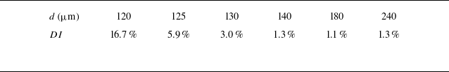


 Open access