2.1. The governing equations

A two-layer set-up with idealized radiation and moist processes is built. It is modified from the fully nonlinear model of Siems et al. (Reference Siems, Bretherton, Baker, Shy and Breidenthal1990) and Mellado et al. (Reference Mellado, Stevens, Schmidt and Peters2009) by adding a Dirac-delta function radiative cooling, as well as changing the basic state buoyancy profile from a local staircase reversal to a global piecewise linear one. The governing equations are expressed with explicit temperature and water species, rather than the mixing fraction formulation. The following four processes are omitted.

1. (i) The background vertical shear which enhances the interfacial mixing (Schulz & Mellado Reference Schulz and Mellado2018).

2. (ii) The droplet settling which reduces the interfacial evaporation by removing droplets near the cloud top (Bretherton, Blossey & Uchida Reference Bretherton, Blossey and Uchida2007; Schulz & Mellado Reference Schulz and Mellado2019).

3. (iii) The lightening effect of water vapour and the loading of liquid water on buoyancy (Austin Reference Austin1995).

4. (iv) The adiabatic expansion and compression of a parcel in vertical motion which is only significant for a sufficiently deep domain, such as the whole stratocumulus layer (Siems et al. Reference Siems, Bretherton, Baker, Shy and Breidenthal1990).

The symbol of all the dimensional variables (but not dimensional parameters) will include a ‘*’. The basic state saturation interface is at $z^*=0$, the lower boundary is a rigid lid at $z^*=-H$ and the upper layer is infinitely deep. Figure 1 shows a schematic diagram of the set-up. The flow is assumed to be Boussinesq. The continuity equation, momentum equation, Clausius-Clapeyron equation, water vapour diagnostic equation, total water equation and thermodynamic equation are

(2.1)\begin{gather} \boldsymbol{\nabla}^* \boldsymbol{\cdot} \boldsymbol{u^*} = 0, \end{gather}

(2.2)\begin{gather} \frac{\partial \boldsymbol{u^*}}{\partial t^*}+ \boldsymbol{u^*} \boldsymbol{\cdot} \boldsymbol{\nabla}^* \boldsymbol{u^*} ={-} \frac{1}{\rho_0} \boldsymbol{\nabla}^* p^* + \frac{g}{T_0}T^* \boldsymbol{k} + \nu \nabla^{*2} \boldsymbol{u^*}, \end{gather}

(2.3)\begin{gather} q^*_{vs}(T^*)=q_{vs0}+\tilde{\lambda} (T^*-T_0), \end{gather}

(2.4)\begin{gather} q_v^*=\min\left\{ q^*_{vs},q^*_t \right\}, \end{gather}

(2.5)\begin{gather} \frac{\partial q^*_t}{\partial t^*}+ \boldsymbol{u}^* \boldsymbol{\cdot} \boldsymbol{\nabla}^* q^*_t ={\kappa} \nabla^{*2} q^*_t\quad \mathrm{with} \ q_t^*=q_v^*+q_l^*, \end{gather}

(2.6)\begin{gather} \frac{\partial T^*}{\partial t^*}+ \boldsymbol{u^*} \boldsymbol{\cdot} \boldsymbol{\nabla}^* T^* - \kappa \nabla^{*2} T^* =\left[ Q^*_{rad} +\frac{L_v{\kappa }}{c_p}\boldsymbol{\nabla}^* q^*_l |_{z^*=z^{*-}_s} \boldsymbol{\cdot} \boldsymbol{n}\delta \left(z^*-z^*_s\right) \right]\nonumber\\ \qquad \qquad \times \delta \left(z^*-z^*_s\right), \end{gather}

where $\boldsymbol {u^*}= u^* \boldsymbol {i} + v^* \boldsymbol {j} + w^* \boldsymbol {k}$ is the three-dimensional velocity vector, $\boldsymbol {i}$, $\boldsymbol {j}$ and $\boldsymbol {k}$ are the three unit vectors of Cartesian coordinate, $\boldsymbol {x^*}= x^* \boldsymbol {i} + y^* \boldsymbol {j} + z^* \boldsymbol {k}$ is the position vector, $\boldsymbol {\nabla }^*=\boldsymbol {i}\partial /\partial x^* + \boldsymbol {j}\partial /\partial y^* + \boldsymbol {k}\partial /\partial z^*$ is the gradient operator, $t^*$ is time and $\min \{\}$ is the minimum operator.

Figure 1.

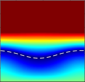
A schematic diagram of the two-layer set-up with (a) the dimensional values and (b) the non-dimensional values. The solid red lines denote temperature profiles, and the solid blue lines denote total water content profiles. The dashed black line denotes the basic state saturation interface. The light blue shadow denotes the saturated region. The deep blue shadow denotes the vertical profile of the liquid water content $q_l$ whose basic state non-dimensional value is $1-\lambda$ at $z=-1$ and $0$ at $z=0$.

The variable $p^*$ is perturbation pressure, $T^*$ is temperature, $q^*_{vs}$ is the saturation vapour content (the mass of saturated vapour in 1 kg of air), $q^*_t$ is the total water content (the total water mass in 1 kg of air) which is the sum of vapour content $q^*_v$ and liquid water content $q_l^*$. The constants $\rho _0$ is the reference density, $\nu$ is the kinematic viscosity, $\kappa$ is the diffusivity shared by $T^*$ and all water species, $L_v$ is the evaporation latent heat and $c_p$ is the isobaric specific heat. For applications to stratocumulus, $\nu$ and $\kappa$ should be viewed as eddy viscosity and diffusivity, respectively. The saturated water vapour content $q^*_{vs}$ is linearized to $T^*$ (Randall Reference Randall1980; Spyksma, Bartello & Yau Reference Spyksma, Bartello and Yau2006), with $\tilde {\lambda }$ as the slope, $T_0$ and $q_{vs0}$ as the reference temperature and saturated water vapour content. They are the radiative-diffusive equilibrium value at $z^*=0$. The constant $Q^*_{rad}$ is the longwave radiative cooling strength (strictly speaking, the radiative flux density expressed in temperature) that depends on the Stefan–Boltzmann law. It is the small penetration depth limit of the simple radiation transfer model of de Lozar & Mellado (Reference de Lozar and Mellado2013). The validity of this radiative representation is discussed in Appendix A. The vector $\boldsymbol {n}$ is the unit vector perpendicular to the saturation interface and points from the saturated region to the unsaturated region. The superscript ‘$-$’ in $z^{*-}_s$ means a tiny distance below $z^*_s$, and vice versa for ‘+’ which will appear later.

The adjustment to thermodynamic equilibrium is assumed to be instantaneous, so the supersaturation (Chandrakar et al. Reference Chandrakar, Cantrell, Krueger, Shaw and Wunsch2020) is not allowed, as shown in (2.4). The assumption of identical diffusivity for $T^*$, $q_v^*$, $q_l^*$ and $q_t^*$ was proposed by Bretherton (Reference Bretherton1987), and has been used in many cloud-top mixing simulations (Siems et al. Reference Siems, Bretherton, Baker, Shy and Breidenthal1990; Mellado et al. Reference Mellado, Stevens, Schmidt and Peters2009; Mellado González Reference Mellado González2010; de Lozar & Mellado Reference de Lozar and Mellado2015; Schulz & Mellado Reference Schulz and Mellado2018). It leads to a drastic simplification: evaporative cooling is determined by the liquid water diffusive flux at the interface. An equivalent argument is shown in (8) of de Lozar & Mellado (Reference de Lozar and Mellado2015) in their mixing fraction formulation. If the diffusivity of temperature and water species are different, diffusion will cause a phase change inside the saturated region. In the real atmosphere the dispersion of droplets is much more complicated than Fickian diffusion (Bois & Kubicki Reference Bois and Kubicki2003).

2.2. Boundary condition

The boundary condition is identical to the simulation of Siems et al. (Reference Siems, Bretherton, Baker, Shy and Breidenthal1990) and Mellado et al. (Reference Mellado, Stevens, Schmidt and Peters2009), except for an infinitely deep upper layer (rather than an upper lid). The lower boundary is a free-slip rigid lid with fixed temperature $T^*$ and total water content $q^*_t$,

(2.7)\begin{equation} \left. \begin{aligned} \left.\frac{\partial u^*}{\partial z^*}\right|_{z^*={-}H} & =\left.\frac{\partial v^*}{\partial z^*}\right|_{z^*={-}H}=w^*|_{z^*={-}H}=0,\\ T^*{|}_{z^*={-}H} & =T_0+\Delta T,\ \ q^*_t{|}_{z^*={-}H}=q_{vs0}+\Delta q_t, \end{aligned} \right\} \end{equation}

where $\Delta T$ and $\Delta q_t$ are the temperature and water content drop across the saturated layer, respectively, and are both positive. In the real atmosphere the downward penetration depth of the mixture produced at the cloud top is limited by its moisture content. The adiabatic compression can make it dry out and then quickly gain buoyancy in the dry adiabatic process, even before reaching the cloud bottom (Siems et al. Reference Siems, Bretherton, Baker, Shy and Breidenthal1990). This effect, which is not explicitly considered in this model, can be implicitly carried by the lower lid. At $z^* \to \infty$, the velocity vanishes, and $T^*$ and $q^*_t$ asymptotically approach a reference linear profile,

(2.8)\begin{equation} \left. \begin{aligned} u^*|_{z^*\to \infty} & = v^*|_{z^*\to \infty} = w^*|_{z^*\to \infty} = 0,\\ T^*|_{z^*\to \infty} & =T_0 -\varGamma_{T\infty}z , \quad q^*_t|_{z^*\to \infty} =q_{vs0}- \varGamma_{q\infty}z, \end{aligned} \right\} \end{equation}

where $\varGamma _{T\infty }$ (negative) and $\varGamma _{q\infty }=\Delta q_t/H$ (positive) are the lapse rate of $T^*$ and $q^*_t$ at $z^*\to \infty$. Strictly speaking, the upper-layer thickness should be smaller than $q_{vs0}/\varGamma _{q\infty }$ to make $q^*_t$ positive. In the real atmosphere $\varGamma _{q\infty }$ is changing with height, and is small outside of the cloud-top mixing layer (Mellado Reference Mellado2017). In this model, switching the water lapse rate to a small value above the convective penetration depth $H_p$ should not influence the result. Thus, we only require $q_t^*$ to be still positive at $z^*=H_p$. Considering that $H_p$ is the neutrally buoyant level of a parcel which ascends adiabatically from the lower boundary, we get $H_p\sim -\Delta T/\varGamma _{T\infty }$. This poses a physical constraint on our model: $H_p\ll q_{vs0}/\varGamma _{q\infty }$ or $-\Delta T/\varGamma _{T\infty } \ll q_{vs0}/\varGamma _{q\infty }$. Furthermore, as $q_{vs0}$ only influences the basic state and does not enter the linear stability analysis, we can always choose a $q_{vs0}$ to satisfy this physical constraint.

2.3. The non-dimensional group

The basic state is in radiative-diffusive equilibrium, without any motion. The basic state variables are denoted with an overline. The Dirac-delta function cooling at the saturation interface makes the basic state temperature profile $\overline {T^*}$ piecewise linear, which decreases with height in the lower saturated layer and increases with height in the upper unsaturated layer. The basic state water content $\overline {q^*_t}$ decreases linearly with height. These basic state profiles will be used to non-dimensionalize the equations.

The governing equation of $\overline {q^*_t}$ is obtained from (2.5). Further using the boundary condition in (2.7) and (2.8), we get

(2.9)\begin{equation} -\kappa \frac{\textrm{d}^2 \overline{q^*_t}}{\textrm{d}{z^*}^2} = 0 \quad \Rightarrow \quad \overline{q^*_t} (z)= q_{vs0} - \varGamma_{q\infty}z^*. \end{equation}

The governing equation of $\overline {T^*}$ and its solution are obtained with (2.3), (2.4), (2.6) and (2.9),

(2.10)\begin{equation} \left. \begin{aligned} -\kappa \frac{\textrm{d}^2 \overline{T^*}}{\textrm{d}{z^*}^2} & = \left( Q^*_{rad} + \frac{L_v\kappa}{c_p}\frac{\textrm{d}\overline{q^*_l}}{\textrm{d}z^*}|_{z^*=0^-} \right) \delta(z^*)\\ \Rightarrow \quad \overline{T^*}(z^*) & = \left\{ \begin{array}{ll} T_0 - \varGamma_{T\infty}z^*, & 0 \le z^*<\infty , \\ T_0 - \varGamma_{Ts}z^*, & -H< z^* \le 0, \end{array} \right. \end{aligned} \right\} \end{equation}

where $\varGamma _{Ts}=\Delta T/H$ (positive) is the $\overline {T^*}$ lapse rate in the saturated layer. The parameters $\varGamma _{Ts}$ and $\varGamma _{T\infty }$ are linked with the radiative and evaporative cooling rate at the interface:

(2.11)\begin{equation} \varGamma_{T_s} = \varGamma_{T\infty} - \frac{1}{\kappa} \left[ Q^*_{rad} - \frac{L_v\kappa}{c_p}\varGamma_{q\infty} \left( 1 - \frac{\tilde{\lambda} \Delta T}{\Delta q_t} \right)\right]. \end{equation}

We choose $\Delta T$ and $\Delta q_t$ as the temperature and water content scale, the saturated layer depth $H$ as the length scale and $H^2/\nu$ as the time scale. The dimensionless variables (without ‘*’) obey

(2.12)\begin{align} \left. \begin{gathered} \boldsymbol{x^*} =\boldsymbol{x} H, \ z^*_s=z_s H,\ t^*=t H^2/\nu ,\\ \boldsymbol{u^*} =\boldsymbol{u}\nu /H, \ p^* =p \rho_0 \nu^2 / H^2,\ T^*-T_0=T \Delta T,\\ q^*_t-q_{vs0}=q_t \Delta q_t, \ q^*_{l}-q_{vs0}=q_{l} \Delta q_t,\ q^*_{v}-q_{vs0}=q_{v} \Delta q_t,\ q^*_{vs}-q_{vs0}=q_{vs} \Delta q_t. \end{gathered} \right\} \end{align}

The problem is controlled by five non-dimensional parameters:

(2.13)\begin{equation} \left. \begin{aligned} Ra=\frac{g (\Delta T/T_0)H^3}{\nu {\kappa }}, \ Pr=\frac{\nu }{{\kappa }},\\ M=\frac{L_v\Delta q_t}{c_p\Delta T},\ Q_{rad}=\frac{Q^*_{rad}}{\Delta T \nu/H} \quad \mathrm{and} \quad {\lambda }=\frac{\tilde{\lambda} \Delta T}{\Delta q_t}. \end{aligned} \right\} \end{equation}

Rayleigh number $Ra$ measures the relative strength of the destabilizing effect of unstable stratification and the stabilizing effect of viscosity and temperature diffusivity. Prandtl number $Pr$ is the ratio of viscosity to temperature and water diffusivity. The $Q_{rad}$ measures the contribution of radiative cooling.

Now, we consider $\lambda$ and $M$ that involve the moisture effect. It is worth noting that their ranges are constrained. The parameter ${\lambda }$ represents the Clausius–Clapeyron equation which influences the interface height $z_s$, as well as the partition between $q_v$ and $q_l$ in the saturated layer which is purely diagnostic under the thermodynamic equilibrium assumption. There must be $\lambda <1$ to guarantee the lower layer is saturated, and $\lambda >0$ to guarantee the monotonicity of saturated vapour pressure on $T$. The parameter $M$ is the ratio of latent to dry enthalpy change across the saturated layer. It can be represented as $M=(L_v/c_p)\tilde {\lambda }\lambda ^{-1}$. The parameter $(L_v/c_p)\tilde {\lambda }$ ranges from 1 to 2 in the 280–290 K temperature range at 900 hPa level which represents the stratocumulus (Randall Reference Randall1980). This, together with $0<\lambda <1$, indicates $M\gtrsim 1$.

Before linearizing the problem, the basic state non-dimensional profiles $\bar {T}$, $\overline {q_t}$, $\overline {q_{vs}}$ and $\overline {q_l}$ are derived from their dimensional expression. The cooling strength at the interface can be further depicted with a parameter $\gamma _T$ which measures the temperature gradient ratio of the upper and lower layers:

(2.14)\begin{equation} \gamma_T \equiv \frac{(\textrm{d}\overline{T^*}/\textrm{d}z^*)_u}{(\textrm{d}\overline{T^*}/\textrm{d}z^*)_s} = \frac{\varGamma_{T\infty}}{\varGamma_{Ts}}. \end{equation}

Here $()_u$ and $()_s$ denote the unsaturated (upper) and saturated (lower) layer property, respectively. The parameter $\gamma _T$ is negative in our case where temperature decreases with height in the lower layer and increases with height in the upper layer. Using (2.3), (2.9), (2.10), (2.12) and (2.14), we get

(2.15)\begin{equation} \left. \begin{gathered} \bar{T}(z) = \left\{ \begin{array}{@{}ll} -\gamma_T z, & 0 \le z<\infty, \\ -z, & -1< z \le 0, \end{array}\right.\quad \overline{q_{l}} =\left\{ \begin{array}{@{}ll} 0, & 0 \le z<\infty, \\ \left( 1-\lambda \right) \bar{T}, & -1< z \le 0, \end{array}\right. \\ \overline{q_t} ={-}z,\quad \overline{q_{vs}} = \lambda \bar{T}. \end{gathered} \right\} \end{equation}

The parameter $\gamma _T$ can be linked to the radiative cooling rate $Q_{rad}$ and the basic state evaporative cooling rate $\overline {Q_{evap}}$ by substituting (2.11) into (2.14), and using the non-dimensional treatment in (2.12) and (2.13):

(2.16)\begin{equation} \overline{Q_{evap}}+Q_{rad} ={-}\frac{1 - \gamma_T}{Pr} \quad \mathrm{with} \ \overline{Q_{evap}}={-}\frac{M(1-\lambda)}{Pr}. \end{equation}

2.4. The linearized governing equation

The disturbance non-dimensional temperature and water content is obtained by subtracting their basic state values from their total values, i.e.

(2.17a–e)\begin{equation} T'=T-\bar{T}, \quad q'_t=q_t-\overline{q_t}, \quad q'_l=q_l-\overline{q_l}, \quad q'_v=q_v-\overline{q_v}, \quad q'_{vs}=q_{vs}-\overline{q_{vs}}. \end{equation}

The non-dimensional gradient operator is defined as $\boldsymbol {\nabla }=\boldsymbol {i}\partial /\partial x + \boldsymbol {j}\partial /\partial y + \boldsymbol {k}\partial /\partial z$. With (2.12), (2.13), (2.15) and (2.17a–e), the dimensional equations (2.1)–(2.6) are non-dimensionalized and linearized,

(2.18)\begin{gather} \boldsymbol{\nabla} \boldsymbol{\cdot} \boldsymbol{u} = 0, \end{gather}

(2.19)\begin{gather} \frac{\partial \boldsymbol{u}}{\partial t} ={-}\boldsymbol{\nabla} p + \frac{Ra}{Pr}T'\boldsymbol{k}+\nabla^2 \boldsymbol{u}, \end{gather}

(2.20)\begin{gather} q'_t|_{z=0}+z_s\left.\frac{\textrm{d}\overline{q_t}}{\textrm{d}z}\right|_{z=0}={\lambda }\left( T'|_{z=0^{-}} + z_s \left.\frac{\textrm{d}\bar{T}}{\textrm{d}z}\right|_{z=0^{-}} \right)={\lambda }\left( T'|_{z=0^{+}} + z_s \left.\frac{\textrm{d}\bar{T}}{\textrm{d}z}\right|_{z=0^{+}} \right), \end{gather}

(2.21)\begin{gather} q_l'=\left[1-\mathcal{H}(z) \right]\left(q_t'-\lambda T'\right), \end{gather}

(2.22)\begin{gather} \frac{\partial q'_t}{\partial t}-w = \frac{1}{Pr}\nabla^2 q'_t, \end{gather}

(2.23)\begin{gather} \frac{\partial T'}{\partial t} = \frac{ 1-\gamma_T}{Pr} z_s \frac{\textrm{d}\delta(z)}{\textrm{d}z} + \frac{M}{Pr}\left( \left.\frac{\partial q'_t}{\partial z} \right|_{z=0} - \lambda \left.\frac{\partial T'}{\partial z}\right|_{z=0^-} \right) \delta(z) + \frac{1}{Pr}\nabla^2 T' \nonumber\\ + w \left[ 1 - (1-\gamma_T) \mathcal{H}(z) \right], \end{gather}

where $\mathcal {H}(z)$ is the Heaviside function. The variables $q'_t$, $q'_{vs}$, $q'_l$, $T'$, $\boldsymbol {u}$ and $z_s$ all have small amplitude. The non-dimensional boundary conditions are obtained from (2.7) and (2.8),

(2.24)\begin{equation} \left. \begin{gathered} \dfrac{\partial u}{\partial z}=\dfrac{\partial v}{\partial z}=w=q'_t=q'_l=T'=0, \quad z={-}1, \\ u=v=w=q'_t=q'_l=T'=0,\quad z\to\infty. \end{gathered} \right\} \end{equation}

Three remarks on the governing equations are made below.

First, the $\textrm {d}\delta (z)/\textrm {d}z$ term on the right-hand side of (2.23) indicates that there is a discontinuity of the small-amplitude $T'$ at $z=0$, which is strictly proved later in (3.6). Physically, it is because the shift of the cooling source produces a small amplitude yet systematic deviation of the temperature profile from the basic state, as illustrated in figure 2(a). The finite-amplitude $T'$ is continuous everywhere, with a sharp transition within $z \in (-z_s,z_s)$. The thickness of the $T'$ transition region reduces to the thickness of the saturation interface at the small-amplitude limit, which is infinitely thin.

Figure 2.

A schematic diagram of (a) the effect of the undulating interface and (b) the effect of non-uniform evaporation at the interface. The solid blue line denotes the perturbed saturation interface. The dashed black line denotes the basic state saturation interface. The vertical blue arrows denote the vertical motion at the interface. The blue patch denotes the cooling anomaly and the red patch denotes the warming anomaly. The circulating red arrows in (a,b) denote the baroclinic torque produced by the interface undulation and non-uniform evaporation, respectively. The solid red lines denote the basic state temperature profiles ($\bar {T}$), and the dotted red lines denote the temperature profiles changed by the interface undulation or the non-uniform evaporation alone.

Second, (2.21) is derived by first transforming (2.4) to $q_l=[1-\mathcal {H}(z-z_s)](q_t-q_{vs})$, and then decomposing it into the basic state and perturbation variables

(2.25)\begin{align} \overline{q_l}+q_l' &=\left[1-\mathcal{H}(z-z_s)\right](\overline{q_t}+q_t'-\overline{q_{vs}}-q_{vs}') \nonumber\\ &\approx\left[1-\mathcal{H}(z)+z_s\delta(z)\right](\overline{q_t}+q_t'-\lambda\bar{T}-\lambda T') \nonumber\\ &\approx\left[1-\mathcal{H}(z) \right](\overline{q_t}-\lambda\bar{T}) + \left[1-\mathcal{H}(z) \right](q_t'-\lambda T') + z_s \delta(z)(\overline{q_t}-\lambda\bar{T}), \end{align}

where we have used $\overline {q_{vs}}=\lambda \bar {T}$ in (2.15) and $q'_{vs}=\lambda T'$, as well as the Taylor expansion of the Heaviside function $\mathcal {H}(z-z_s) \approx \mathcal {H}(z)-z_s\delta (z)$. Because $\overline {q_t}-\lambda \bar {T}=0$ at $z=0$, the third term on the right-hand side of (2.25) vanishes. Because $\overline {q_l}=[1-\mathcal {H}(z) ](\overline {q_t}-\lambda \bar {T})$ as is indicated by (2.15), the perturbation part of (2.25) becomes (2.21).

Third, (2.23) is derived by first linearizing $\boldsymbol {\nabla } q_l |_{z=z^{-}_s} \boldsymbol {\cdot } \boldsymbol {n}$ to $\partial q_l/\partial z|_{z=z_s^-}$, and then using Taylor expansion of the Dirac-delta function $\delta (z-z_s)\approx \delta (z)-z_s\,\textrm {d}\delta (z)/\textrm {d}z$ to linearize the interfacial cooling term around $z=0$. The derivative and Taylor expansion of a Dirac-delta function is defined by considering it as a generalized function (a distribution). See appendix C.4 of the book of Pope (Reference Pope2000) for a reference. The Taylor expansion of the Heaviside function also exists, because it is the integral of the Taylor expansion of a Dirac-delta function. The detail of the expansion of the Dirac-delta function term in the non-dimensional version of (2.6) is as follows:

(2.26) \begin{align} & \left(Q_{rad} + \frac{M}{Pr}\boldsymbol{\nabla} q_l |_{z=z^{-}_s} \boldsymbol{\cdot} \boldsymbol{n} \right) \delta(z-z_s) \nonumber\\ &\quad \approx \left[ Q_{rad} + \frac{M(1-\lambda)}{Pr}\frac{\textrm{d} \overline{q_t}}{\textrm{d} z} + \left.\frac{M}{Pr} \frac{\partial q'_l}{\partial z}\right|_{z=0^-} \right] \left( \delta(z) - z_s \frac{\textrm{d}\delta(z)}{\textrm{d}z} \right) \nonumber\\ &\quad \approx \left[ Q_{rad} + \frac{M(1-\lambda)}{Pr}\frac{\textrm{d} \overline{q_t}}{\textrm{d} z} \right] \delta(z) - \left[ Q_{rad} + \frac{M(1-\lambda)}{Pr}\frac{\textrm{d} \overline{q_t}}{\textrm{d} z} \right] \frac{\textrm{d}\delta(z)}{\textrm{d}z}z_s \nonumber\\ &\qquad + \frac{M}{Pr}\left( \left.\frac{\partial q'_t}{\partial z}\right|_{z=0} - \lambda \left.\frac{\partial T'}{\partial z}\right|_{z=0^-} \right) \delta(z) \nonumber\\ &\quad \approx \underbrace{-\frac{1-\gamma_T}{Pr} \delta(z)}_{\textit{basic state}} + \underbrace{\frac{1-\gamma_T}{Pr} \frac{\textrm{d}\delta(z)}{\textrm{d}z}z_s}_{\textit{interface undulation}} + \underbrace{\frac{M}{Pr}\left( \left.\frac{\partial q'_t}{\partial z}\right|_{z=0} - \lambda \left.\frac{\partial T'}{\partial z} \right|_{z=0^-} \right) \delta(z)}_{\textit{non-uniform evaporation}}. \end{align}

Here we have used (2.16) and (2.21). The quantities $\partial q'_l / \partial z|_{z=0^-}$, $\partial q'_t / \partial z|_{z=0}$, $\partial T' / \partial z|_{z=0^-}$ and $z_s$ all have small amplitude, so the product between them vanish in the linear analysis. On the right-hand side of (2.26), the first term denotes the basic state part, the second term denotes the interface undulation which produces a vertical dipole heating pattern, and the third term denotes the horizontally non-uniform evaporation which produces a monopole heating pattern. The basic state part leads to a piecewise linear $\bar {T}$ and, therefore, a piecewise constant $\textrm {d}\bar {T}/\textrm {d}z$, which corresponds to the $-w \,\textrm {d}\bar {T}/\textrm {d}z=w [ 1 - (1-\gamma _T) \mathcal {H}(z) ]$ term in (2.23).

3.1. The eigenvalue problem

As the non-uniform evaporation and interface undulation take the form of a Dirac-delta function and its derivative in (2.23), their influence is concentrated near the saturation interface. Thus, compared with the fixed TRBC, the moisture effect only influences the matching condition. The procedure in this subsection is a standard practice that follows Ogura & Kondo (Reference Ogura and Kondo1970), except the matching conditions of $\hat {T}$ and $D\hat {T}$ which are novel.

The normal mode solution is

(3.1)$$\begin{align} \{u,\ v,\ w,\ p,\ T', \ q'_t,\ q'_l, \ z_s \} & =\{\hat{u}(z),\ \hat{v}(z),\ \hat{w}(z),\ \hat{p}(z),\ \hat{T}(z),\ \hat{q}_t(z),\ \hat{q}_l(z),\ \hat{z}_s \} \nonumber\\ & \quad \times \exp\left[\textrm{i}(k_xx+k_yy)\right] \exp\left(\sigma t\right), \end{align}$$

where $k_x$ is the $x$-direction wavenumber, $k_y$ is the $y$-direction wavenumber, $\sigma \equiv {\sigma }_r+\textrm {i}{\sigma }_i$ is the complex growth factor, where $\sigma _r$ denotes the growth rate and $\sigma _i$ denotes the oscillation frequency. The z-dependent variables with a ‘hat’ denote the eigenfunctions. By substituting (3.1) into (2.18), (2.19) and (2.23), a sixth-order ordinary differential equation (ODE) of $\hat {w}$ is obtained:

(3.2)\begin{equation} \left(Pr\sigma +K^2-D^2\right)\left(\sigma +K^2-D^2\right)(K^2-D^2)\hat{w}=\left\{ \begin{array}{ll} \gamma_T Ra K^2\hat{w}, & 0< z<\infty, \\ Ra K^2\hat{w}, & -1 < z < 0, \end{array} \right. \end{equation}

where $K^2\equiv k^2_x+k^2_y$, $D\equiv \textrm {d} /\textrm {d} z$. The derivative of the eigenfunctions will use notation $D$ rather than $\textrm {d}/\textrm {d}z$. At $z=-1$, the non-penetrative and free-slip velocity boundary condition, as well as the Dirichlet temperature boundary condition $T'|_{z=-1}=0$ that are adapted from (2.7) to yield

(3.3)\begin{equation} \hat{w}=D^2\hat{w}=D^4\hat{w}=0,\quad z={-}1. \end{equation}

As (3.2) have constant coefficients, obey the homogeneous lower boundary condition shown in (3.3) and the natural boundary condition at $z\to \infty$, we have

(3.4)\begin{equation} \hat{w}(z)=\left\{ \begin{array}{ll} \displaystyle\sum^6_{m=4}{a_m{e^{{-}p_m z}\ }}, & 0< z<\infty, \\ \displaystyle\sum^3_{m=1}{a_m{\mathrm{sinh} [p_m(z+1)]\ }}, & -1< z<0. \end{array} \right. \end{equation}

Here $a_m$, $m=1,2,3,4,5,6$ are the amplitude coefficients, $p_m$ are the eigenvalues. Substituting (3.4) into (3.2), and viewing $\sigma$, $Ra$ and $K^2$ as coefficients, a complex cubic equation of $p^2_m$ is obtained and analytically solved using the method of Lebedev (Reference Lebedev1991). As the sign of $p_m$ is not constrained by the cubic equation, we choose the $p_m$ with a positive real part.

The six coefficients $a_m$ need to be determined by six matching conditions at $z=0$. The first four are the continuity of vertical velocity $w$, horizontal velocity $u$ and $v$, the non-dimensional tangential stress components $(\partial u/\partial z+\partial w/\partial x)$ and $(\partial v/\partial z+\partial w/\partial y)$, and pressure $p$. Using the normal mode form of (2.18) and (2.19), a few lines of algebra yield

(3.5)\begin{equation} D^n\hat{w}{|}_{z=0^-}=D^n\hat{w}{|}_{z=0^+},\quad n=0,\ 1,\ 2,\ 3. \end{equation}

The remaining two conditions are about the disturbance temperature $T'$ and heat flux $Pr^{-1} \partial T'/\partial z$. Unlike the fixed TRBC where $\hat {T}$ and $D\hat {T}$ are continuous at $z=0$, §§ 3.2 and 3.3 will show that it is not the case for the free TRBC due to the interface undulation and the non-uniform evaporation there. The full solution procedure of the eigenvalue problem is shown in Appendix B.

3.2. The effect of undulating interface

The first term on the right-hand side of (2.23) denotes the interface undulation. First, we study how the small-amplitude interface displacement $\hat {z}_s$ produces a jump of $\hat {T}$ at $z=0$. Let $\epsilon$ be a small positive constant. The following double integral is performed on (2.23), within a small slot encompassing the interface. All terms vanish except the vertical diffusion term which has the highest order, and the $\textrm {d}\delta (z)/\textrm {d}z$ term which changes most abruptly:

(3.6)\begin{gather} \frac{1-\gamma_T}{Pr} \hat{z}_s\int^{\epsilon}_{-\epsilon} \int^{z'}_{-\epsilon} \frac{\textrm{d}\delta(z)}{\textrm{d}z}\,\textrm{d}z\,\textrm{d}z' \sim{-} \frac{1}{Pr}\int^{\epsilon}_{-\epsilon} \int^{z'}_{-\epsilon} D^2\hat{T}\,\textrm{d}z\,\textrm{d}z' \nonumber\\ \Rightarrow \quad \frac{1-\gamma_T}{Pr} \hat{z}_s + \frac{1}{Pr} \left(\hat{T}|_{z=0^+} - \hat{T}|_{z=0^-} \right) = 0. \end{gather}

Another more straightforward way to derive (3.6) is to use the interfacial temperature continuity $T|_{z=z_s^+} = T|_{z=z_s^-}$ and perform Taylor expansion of $T$ near $z=0$, as has been employed by Hsieh (Reference Hsieh1972) in studying liquid–gas flow. The parameter $Pr$ appears on both terms of the second line of (3.6) and can be eliminated.

Then, we consider the Clausius–Clapeyron equation that determines $z_s$. At the saturation interface, there is $q_{vs} = q_t$. The normal mode form of (2.20) yields

(3.7)\begin{gather} \hat{q}_t|_{z=0}+\frac{\textrm{d}\overline{q_t}}{\textrm{d}z}\hat{z}_s = \lambda \left( \hat{T}|_{z=0^{-}}+ \left.\frac{\textrm{d}\bar{T}}{\textrm{d}z}\right|_{z=0^{-}}\hat{z}_s \right) = \lambda \left( \hat{T}|_{z=0^{+}}+ \left.\frac{\textrm{d}\bar{T}}{\textrm{d}z}\right|_{z=0^{+}}\hat{z}_s \right) \nonumber\\ \Rightarrow \quad \hat{z}_s = \frac{\hat{q}_t|_{z=0}-\lambda \hat{T}|_{z=0^-}}{1-\lambda} = \frac{\hat{q}_t|_{z=0}-\lambda \hat{T}|_{z=0^+}}{1-\lambda \gamma_T}. \end{gather}

Fielder (Reference Fielder1984) has derived an expression similar to (3.7) to find the cloud bottom undulation magnitude, where he considered the matching between a well-mixed sub-cloud layer and a well-mixed cloud layer.

The normal mode form of (2.18) and (2.19) are manipulated to represent $\hat {T}$ with $\hat {w}$:

(3.8)\begin{equation} \hat{T}=\frac{Pr}{RaK^2}\left( D^2-K^2-\sigma \right) \left(D^2-K^2\right) \hat{w}. \end{equation}

Substituting (3.7) and (3.8) into (3.6), we obtain the matching condition of $\hat {T}$:

(3.9)\begin{gather} \hat{T}|_{z=0^+} \frac{1-\lambda}{1-\lambda \gamma_T} - \hat{T}|_{z=0^-} =\frac{Pr}{Ra K^2} \left( D^2-K^2-\sigma \right) \left( D^2-K^2 \right) \nonumber\\ \times \left( \hat{w}{|}_{z=0^+} \frac{1-\lambda}{1-\lambda \gamma_T} - \hat{w}{|}_{z=0^-} \right) = \underbrace{ -\frac{1-\gamma_T}{1-\lambda \gamma_T} }_{\eta_T} \hat{q}_t|_{z=0}, \end{gather}

where $\eta _T$ is a negative constant. The $\hat {w}{|}_{z=0^+}$ and $\hat {w}{|}_{z=0^-}$ on the second line of the right-hand side denote the derivative value of $\hat {w}$ at $z=0^+$ and $z=0^-$.

The quantity $\hat {q}_t|_{z=0}$ is obtained by solving $q'_t$ as an advective-diffusive tracer driven by $w$. The normal mode form of (2.22) is a second-order ODE of $\hat {q}_t$:

(3.10)\begin{equation} D^2\hat{q}_t-\left(K^2+\sigma Pr\right)\hat{q}_t={-}\hat{w}Pr \quad \mathrm{with} \ \hat{q}_t{|}_{z={-}1}=\hat{q}_t{|}_{z \to\infty}=0. \end{equation}

It is solved with the method of variation of parameter in Appendix C. For $\sigma =0$, (3.10) can be viewed as the normal mode form of a Poisson equation with $-\hat {w}Pr$ as the source term. Thus, when $\hat {w}$ is a real function (no phase tilt with height), $\hat {q}_t$ is real and has the same sign as $\hat {w}$. In other words, there is always positive $q'_t|_{z=0}$ at the updraft region for a neutral mode due to vertical advection.

The physical influence of the undulating interface is briefly analysed here, and illustrated in figure 2(a). The updraft at the saturation interface pushes the air at the interface upward. These parcels are the coldest air in the vertical air column. The temperature field adjusts to the rising dome through diffusion, so the result is a cold anomaly at the upper layer and a warm anomaly at the lower layer, and vice versa in a valley produced by a downdraft. This produces a vertical dipole buoyancy anomaly, which corresponds to two undulation-induced torques which are in the opposite sign. A qualitatively similar yet more singular pattern can be produced by the interface undulation in a three-layer Rayleigh–Taylor instability model (Mellado et al. Reference Mellado, Stevens, Schmidt and Peters2009). We note that the torque below the interface is in the same direction as the lower-layer convective cell (also a torque), which is generated by the unstable stratification. Because the main body of the convective cell is below the interface, the cell receives a more positive influence from the interfacial torque right below the interface than the negative influence from the torque right above the interface. Thus, the interface undulation is a destabilizing factor. A stricter explanation based on energetics is given in § 4.5.

3.3. The effect of non-uniform evaporation at the interface

The second term on the right-hand side of (2.23) denotes the non-uniform liquid water diffusion and, therefore, evaporative cooling at the interface. It induces a jump of perturbation heat flux and, therefore, $D\hat {T}$ at $z=0$. This term is the key to reproduce the deformation-induced anomalous evaporative cooling at a ‘flame front’ (the interfacial ridge lifted by the updraft) described by Siems et al. (Reference Siems, Bretherton, Baker, Shy and Breidenthal1990) and Mellado et al. (Reference Mellado, Stevens, Schmidt and Peters2009). The author is unaware of any previous work that addresses the influence of the deformation-induced anomalous evaporation on the interfacial instability.

Equation (2.23) indicates that the matching condition for heat flux in normal mode form is

(3.11)\begin{equation} D\hat{T}{\left.{}\right|}_{z=0^+}-D\hat{T}{|}_{z=0^-} ={-}M \left( D\hat{q}_t|_{z=0} - \lambda D\hat{T}|_{z=0^-} \right). \end{equation}

Substituting (3.8) into (3.11), we get the matching condition represented with $\hat {w}$:

(3.12)\begin{gather} \frac{Pr}{Ra K^2} \left( D^2-K^2-\sigma \right) \left( D^2-K^2 \right) D \left[\hat{w}|_{z=0^+} - (1+\lambda M) \hat{w}|_{z=0^-} \right] \nonumber\\ ={-}M D \hat{q}_t|_{z=0}. \end{gather}

As in § 3.2, the $\hat {w}{|}_{z=0^+}$ and $\hat {w}{|}_{z=0^-}$ on the left-hand side denote the value of the derivatives of $\hat {w}$ at $z=0^+$ and $z=0^-$. The expression of $D\hat {q}_t|_{z=0}$ is documented in Appendix C.

In § 4 the eigenfunctions of the neutral mode show that in most cases there is always $\partial q'_l/\partial z|_{z=0^-}<0$ at the updraft region ($w|_{z=0}>0$), primarily due to the squeezing of the $q_t$ contour surfaces near the interface. The detailed physical understanding and constraint are to be discussed in § 4.4. Figure 2(b) illustrates the physical influence of non-uniform evaporation. There is more evaporative cooling in the updraft region than in the downdraft region, so the baroclinic torque produced by the non-uniform evaporation is opposite to the torque produced by the lower-level unstable stratification. Thus, the non-uniform evaporation is stabilizing. It is worth noting that $M$ only influences the instability via (3.11), not directly relevant to the interface undulation. Thus, a larger $M$ directly means a stronger non-uniform evaporation.

4.1. The investigation strategy

Three reference tests of the linear stability problem are performed.

1. (i) The Ref-F test which is a fixed TRBC test that uses $\gamma _T=-2.5$ and $Pr=1$. The matching condition uses $\hat {T}|_{z=0^+}=\hat {T}|_{z=0^-}$ and $D\hat {T}|_{z=0^+}=D\hat {T}|_{z=0^-}$.

2. (ii) The Ref-E test with purely evaporative cooling that uses $M=6.364$, $\lambda =0.45$, $\gamma _T=-2.5$ and $Pr=1$ (corresponding to $Q_{rad}/\overline {Q_{evap}}=0$).

3. (iii) The Ref-ER test with both evaporative and radiative cooling that uses $M=3$, $\lambda =0.45$, $\gamma _T=-2.5$ and $Pr=1$ (corresponding to $Q_{rad}/\overline {Q_{evap}}=1.12$).

Sensitivity tests are performed around Ref-ER, with an emphasis on studying the sensitivity to $Q_{rad}/\overline {Q_{evap}}$ by changing $\lambda$ and $\gamma _T$. The Ref-E test can be regarded as a special sensitivity test of the Ref-ER test with a larger $M$, which directly means a stronger non-uniform interfacial evaporation. Though this parameter set does not correspond to a specific state of real stratocumulus which is turbulent, it is an idealized state where the convective instability in the saturated layer, interfacial instability and upper-layer stratification all play a role. Only the marginal stability curve is studied in this section to understand the physical mechanism. Thus, $Ra$ is to be solved, rather than prescribed. In § 5 the weakly supercritical (linearly unstable) regime is briefly explored with nonlinear numerical simulation. The neutral mode might represent the large eddy component of a turbulent flow, with the small-scale eddies parameterized as the diffusivity (Zhou, Simon & Chow Reference Zhou, Simon and Chow2014; Thuburn & Efstathiou Reference Thuburn and Efstathiou2020). We leave the careful investigation of the relevance to the turbulent stratocumulus for future works.

The critical (marginally stable) $Ra$ is defined as $Ra_c$. The problem is horizontally isotropic, so there is no need to split the horizontal total wavenumber $K$ into $k_x$ and $k_y$. On a marginal curve, the minimum $Ra_c$ is defined as $Ra_{cm}$ and the corresponding $K$ is $K_{cm}$. For the single layer Rayleigh–Bénard convection at $Pr=1$, the existence of minimum $Ra_c$ can be heuristically understood as the competition between the destabilizing effect of the inviscid unstable gravity wave component, and the stabilizing effect of the diffusive and viscous component (Thuburn & Efstathiou Reference Thuburn and Efstathiou2020). The supposed growth rate of the unstable gravity wave increases mildly with $K$ and asymptotically approaches $(Ra/Pr)^{1/2}$, which is the modulus of the non-dimensional imaginary Brunt–Väisälä frequency. The damping rate of diffusion increases as $K^2$. Thus, $Ra_{cm}$ must be achieved at a finite $K=K_{cm}$. It will be shown that in this problem, a smaller $Ra_{cm}$ is mostly accompanied with a smaller $K_{cm}$, similar to the fixed TRBC problem (Ogura & Kondo Reference Ogura and Kondo1970). Qualitatively speaking, a smaller $Ra_{cm}$ means a smaller imaginary Brunt–Väisälä frequency, so less diffusion and therefore a lower $K_{cm}$ is needed to balance it.

By calculating the growth rate of various $Ra$ in the parameter space around the reference test, we have not found any growing or neutral oscillatory mode ($\sigma _r \ge 0$, $\sigma _i \neq 0$). Thus, we let the solver (introduced in Appendix B) only search across stationary modes ($\sigma _i = 0$) in all the tests. Whitehead (Reference Whitehead1968) has shown that an unstable or neutral oscillatory mode does not exist for the fixed TRBC problem (the principle of exchange of stability), but a rigorous proof is hard for our free TRBC problem. For the stationary mode, we arbitrarily set the phase by letting $\hat {w}$ be a real function with positive value in the lower layer. With this setting, the normal mode form of (2.18)–(2.23) show that all the eigenfunctions in (3.1) are real functions except $\hat {u}(z)$ and $\hat {v}(z)$. These real-value eigenfunctions are proportional to the physical space variables at an updraft column.

In Appendix D we introduce the novel finding that the purely evaporative cooling case yields an identical marginal stability curve (for the neutral mode) and growth rate (for the growing mode) to the corresponding fixed TRBC case (using the same $\gamma _T$ and $Pr$ but for $\hat {T}|_{z=0^+}=\hat {T}|_{z=0^-}$ and $D\hat {T}|_{z=0^+}=D\hat {T}|_{z=0^-}$). In § 4.5 it is explained as the cancellation between the effect of the interface undulation and non-uniform evaporation with an argument of energetics.

4.2. The lowest $Ra_c$ neutral mode of the two reference tests

Figure 3(a) shows the marginal stability curve of the Ref-F test, Ref-E test and Ref-ER test. The curve of the Ref-E test completely overlaps with that of the Ref-F test, which is strictly proved in Appendix D. The Ref-ER test has a lower $Ra_{cm}$ and a smaller $K_{cm}$. We explain this more unstable behaviour as a smaller $M$ (larger $Q_{rad}/\overline {Q_{evap}}$) which makes the stabilizing effect of the non-uniform evaporation weaker than the destabilizing effect of the interface undulation.

Figure 3.

The marginal stability curve. (a) The solid red line is the Ref-F test, the dashed blue line is the Ref-E test, the solid black line is the Ref-ER test and the dashed green line is the Ref-ER test with the additional non-uniform radiative cooling at the interface (discussed in Appendix A). (b) The solid blue line and solid red line denote the $\lambda =0$ and $\lambda =1$ tests respectively for the reference $\gamma _T =-2.5$. The dashed blue line and dashed red line denote the corresponding tests for a double $\gamma _T$. In the code, we use $\lambda =10^{-10}$ to approximate $\lambda =0$ and $\lambda = 1-10^{-10}$ to approximate $\lambda =1$, to avoid dividing by zero. (c) The solid blue line and dashed red line denote changing $Pr$ to 0.5 and 2 times of their reference value ($Pr=1$), respectively. All tests in (b) and (c) are free TRBC tests with radiative cooling.

The eigenfunctions and the reconstructed flow field in figure 4 show that, for all tests, there is a primary cell confined within the saturated layer. The Ref-E and Ref-ER tests have a less penetrative primary cell but a more prominent secondary upper cell than the Ref-F test, due to the baroclinic torque produced by the interface undulation. Though the Ref-E test and the Ref-F test have the same ${Ra}_{cm} = 381.82$ and $K_{cm} = 1.90$, their eigenfunctions and therefore flow patterns are different. For the Ref-E and Ref-ER tests, the interface ${z=z_s}$ is raised at the updraft branch. Whether it is flatter than the $q_t$ contour lines is hard to see from this figure due to a ‘technical issue’ in the plotting: too large an amplitude violates the small-amplitude assumption, and too small an amplitude is hard to observe. This point will be carefully discussed in § 4.3 and the interface will be shown to be no steeper. As there is $D{\hat {q}_l}| _{z=0^-}<0$ in figure 4 for the Ref-E and Ref-ER tests, the perturbation liquid water gradient is negative at the updraft. This corresponds to a larger $q_l$ gradient at the updraft ridge of the interface, which produces more evaporation and explains the stabilizing effect of the non-uniform evaporation.

Figure 4.

(a) The vertical profile of eigenfunction $\hat {w}$ (black line), $\hat {T}$ (red line) and $\hat {q}_t$ (blue line) for the Ref-F test. The magnitude is chosen by letting the maximum value of $\hat {w}$ be unit. The eigenfunctions $\hat {T}$ and $\hat {q}_t$ are further multiplied by $2 K_{cm}^2/Pr$ to make their magnitude close to unit, because (2.22) and (2.23) are close to advection–diffusion equations. (b) The reconstructed 2-D $x$-$z$ flow field, with $k_x=K_{cm}$. The magnitude of $\hat {w}$ is set as $\max \{|\hat {w}|\}=2$. The velocity vector is shown as the arrows. The $q_t$ (as a passive tracer in the fixed TRBC) is shown as the contour lines, with each line corresponding to an increment of 0.4. The domain width ‘4’ is arbitrary and does not mean a wavelength. (c) The same as (a), but for the Ref-E test, and with an additional $\hat {q}_l$ profile (green line) which is also multiplied by $2 K_{cm}^2/Pr$. (d) The same as (b), but for the Ref-E test, and the additional dashed white line denotes the interface $z_s$. Plots (e,f) are the same as (c,d), but for the Ref-ER test where both evaporative and radiative cooling are present. Results are shown for (a) $\text {Ref-F}\ Ra_{cm} =381.82\ K_{cm}=1.90$; (b) $\text {Ref-F}\ q_t$; (c) $\text {Ref-E}\ Ra_{cm} =381.82\ K_{cm}=1.90$; (d) $\text {Ref-E}\ q_t$; (e) $\text {Ref-ER}\ Ra_{cm} =263.46\ K_{cm}=1.58$; (f) $\text {Ref-ER}\ q_t$.

4.3. The dynamics of interface undulation

In the absence of radiative cooling ($Q_{rad}/\overline {Q_{evap}}=0$) the interface has constant $T=0$ and $q_t=0$ ($\hat {z}_s=\hat {q}_t|_{z=0}$ for any $\lambda$), a property due to the synchronous evolution of $q_t$ and enthalpy $h=(c_pT^*+L_vq^*_v-c_pT_0-L_vq_{vs0})/(c_p\Delta T)=T+Mq_v$. This was pointed out in an equivalent thermodynamic framework by Mellado et al. (Reference Mellado, Stevens, Schmidt and Peters2009), and is derived with our thermodynamic framework in Appendix D. As $\hat {q}_t|_{z=0}$ must be positive at the updraft, as has been discussed in § 3.2, the saturation interface should rise at the updraft due to the moisture increment.

What is the physical mechanism for $T$ to be fixed in the $Q_{rad}/\overline {Q_{evap}}=0$ case? We explain it as a competition: for an updraft, the warming tendency due to the change of interface height is balanced by the cooling tendency due to the extra evaporative cooling at the interface. The warming tendency can be understood with an idealized purely diffusive problem of $T$, with the interface cooling rate fixed. Suppose $z_s$ moves upward at an updraft due to interface undulation. As the upper level is infinitely thick, the vertical thermal diffusion strongly adjusts the upper level temperature profile to the new diffusive-equilibrium profile, which makes $T|_{z=z_s}$ rise. The full adjustment is impossible due to the damping by horizontal diffusion.

What if radiative cooling is considered? Equation (2.16) shows that the $Q_{rad}/\overline {Q_{evap}}$ is larger for a smaller $M$, larger $\lambda$ or larger $-\gamma _T$. The suppression of the instability by a larger $M$ has been discussed at the end of § 3.3, so we focus on $\lambda$ and $\gamma _T$. We hypothesize that the addition of radiative cooling leads to a stronger interface undulation relative to the non-uniform evaporation, so the anomalous cooling at the updraft ridge of the interface is weaker compared with the warming tendency. Thus, the interfacial temperature $T|_{z=z_s}$ should rise more above the basic state value $T=0$, and the Clausius–Clapeyron equation indicates that the saturation interface should fall behind the $q_t=0$ contour line ($\hat {z}_s/\hat {q}_t|_{z=0}<1$). The hypothesis is confirmed in figure 5(a), which shows that $\hat {z}_s/\hat {q}_t|_{z=0}$ decreases as $\lambda$ or $-\gamma _T$ increases. In particular, there is $\hat {z}_s=\hat {q}_t|_{z=0}$ for the $\lambda =0$ case, because the Clausius–Clapeyron equation (3.7) is independent of temperature when $\lambda =0$. The $\hat {z}_s=\hat {q}_t|_{z=0}$ is a property shared by the $Q_{rad}/\overline {Q_{evap}}=0$ (yet $\lambda \neq 0$) case. The analysis leads to an inference: even though radiative cooling enhances interface undulation, the decrease of $\hat {z}_s/\hat {q}_t|_{z=0}$ means that it is self-limiting.

Figure 5.

(a) The change of $\hat {z}_s/\hat {q}_t|_{z=0}$ with $\lambda$ for two $\gamma _T$ values, with other parameters identical to the Ref-ER test. The solid blue line denotes the test using the reference value $\gamma _T=-2.5$, and the solid red line denotes the double $\gamma _T$ test. The dashed blue and dashed red lines denote $(1-\lambda \gamma _T)^{-1}$ for the normal and double $\gamma _T$ test, respectively, which are the theoretical estimates of the lower bound (abbreviated as LB). (b) The dependence of $D\hat {q}_l|_{z=0^-}/D\hat {q}_t|_{z=0}$ on $Q_{rad}/\overline {Q_{evap}}$ (solid blue line), performed by changing $\gamma _T$ while fixing $\lambda$ and $M$ to the Ref-ER test value. The dashed blue line is $(1-\lambda )$ which is an estimated lower bound of $D\hat {q}_l|_{z=0^-}/D\hat {q}_t|_{z=0}$.

In fact, a quantitative lower bound of $\hat {z}_s/\hat {q}_t|_{z=0}$ can be found. Note that $\hat {z}_s$ can be expressed with either $\hat {T}_{z=0^-}$ or $\hat {T}_{z=0^+}$ in (3.7). As long as $\hat {z}_s$ is positive (the interface rises at the updraft), both the movement of the interfacial cooling source and the direct vertical advection of the basic state temperature make $\hat {T}_{z=0^-} \gtrsim 0$ and $\hat {T}_{z=0^+} \lesssim 0$. Substituting this argument into (3.7), and combining it with the physical argument $\hat {z}_s\lesssim \hat {q}_t|_{z=0}$, we obtain a range estimation of $\hat {z}_s$:

(4.1)\begin{equation} \frac{\hat{q}_t|_{z=0}}{1-\lambda \gamma_T} \lesssim \hat{z}_s \lesssim \hat{q}_t|_{z=0}. \end{equation}

The lower bound is plotted as the dashed lines in figure 5(a). Though this constraint is loose, the lower bound does grasp the decrease of $\hat {z}_s$ with $\lambda$, as well as a faster decrease for a higher $-\gamma _T$ (with fixed $M$ and $Pr$).

4.4. The liquid water gradient near the interface

Equation (2.23) shows that the sign of $\partial q'_l/\partial z$ near the interface depends on $\partial q'_t/\partial z$ and $\partial T'/\partial z$. As the basic state $q_t$ and $T$ in the lower layer are both decreasing with height, there is a positive $q_t$ and $T$ anomaly at the updraft region. The flow is horizontally divergent as the updraft intersects the interface, so the $q_t$ contour surfaces are squeezed and there is a negative $\partial q'_t/\partial z$, as has been discussed in § 3.3. The rising of the interface cooling source also induces a warming anomaly right below the interface (e.g.  figure 2a), which locates above the peak warming anomaly induced by the upward advection of the unstable basic state. Thus, the negative $D\hat {T}|_{z=0^-}$ should rise towards zero, as can be seen by comparing figures 4(c) and 4(e).

This can be partly quantified. We start from the $Q_{rad}/\overline {Q_{evap}}=0$ case introduced in Appendix D, where (D7) shows $\hat {q}_t=\hat {T}$ for $z<0$. This indicates

(4.2)\begin{equation} D\hat{q}_l|_{z=0^-}=\left(1-\lambda \right)D\hat{q}_t|_{z=0}\quad \mathrm{for} \ Q_{rad}/\overline{Q_{evap}}=0. \end{equation}

When radiative cooling is incorporated and gradually raised by increasing $-\gamma _T$, the $\hat {T}$ jump at $z=0$ should increase according to (3.6). Thus, we expect that as $-\gamma _T$ increases, $D\hat {q}_l|_{z=0^-}$will approach $D\hat {q}_t|_{z=0}$. This argument and (4.2) lead to a constraint of $D\hat {q}_l|_{z=0^-}/D\hat {q}_t|_{z=0}$:

(4.3)\begin{equation} 1-\lambda \lesssim \frac{D\hat{q}_l|_{z=0^-}}{D\hat{q}_t|_{z=0}} \lesssim 1. \end{equation}

For a $-\gamma _T$ as large as $20$ (very strong interfacial undulation), $D\hat {T}|_{z=0^-}$ only marginally exceeds $0$ and $D\hat {q}_l|_{z=0^-}/D\hat {q}_t|_{z=0}$ marginally exceeds $1$. We have not figured out the mechanism of this asymptotic behaviour. Equation (4.3) is verified in figure 5(b) which shows that $D\hat {q}_l|_{z=0^-}/D\hat {q}_t|_{z=0}$ does increase mildly with increasing $Q_{rad}/\overline {Q_{evap}}$ (performed by changing $\gamma _T$ and fixing $\lambda$), with $(1-\lambda )$ as its lower bound. This indicates a coupling of the two effects: a stronger interface undulation tends to enhance the non-uniform evaporation to some extent. Unfortunately, (4.3) is not accurate enough to include $\gamma _T$.

With (4.1) and (4.3) in hand, we try to answer whether $\lambda$ is a destabilizing factor or not. First, we look at the marginal curve of different $\lambda$ for fixed $\gamma _T$. Figure 3(b) shows that for the reference value $\gamma _T=-2.5$, a larger $\lambda$ significantly destabilizes the system. For double $\gamma _T$, however, a larger $\lambda$ weakly stabilizes the system. This indicates that a larger $-\gamma _T$ (stronger upper-layer stratification) gradually shifts $\lambda$ from a destabilizing factor to a stabilizing one. Physically, this is due to two competing factors. For given $-\gamma _T$, a larger $\lambda$ suppresses $\hat {z}_s$ and therefore weakens the interface undulation as shown in (4.1), but it also weakens the non-uniform evaporation as shown in (4.3) due to a smaller magnitude of liquid water gradient. The dependence of the relative strength of the two factors on $\gamma _T$ is not quantitatively constrained at present.

4.5. The relative importance of interface undulation and non-uniform evaporation

The relative strength of the destabilizing effect of the undulating interface and the stabilizing effect of non-uniform evaporation is quantified by comparing their relative contribution to the tendency of the vertical buoyancy flux $\overline {wT'}$. Here the overline on perturbation quantities denotes horizontal average in a wavelength. Multiplying $w$ to (2.23), multiplying $T'$ to the $w$ component of (2.19), and then summing them up and performing a horizontal wavelength average, we get

(4.4)\begin{gather} \frac{\partial \overline{wT'}}{\partial t} = \overline{w \left( \frac{\partial T}{\partial t} \right)_{IU}} + \overline{w \left( \frac{\partial T}{\partial t} \right)_{NE}} + \mathrm{etc.}, \end{gather}

(4.5a,b)\begin{gather} \overline{w \left( \frac{\partial T}{\partial t} \right)_{IU}} \equiv \hat{w} \frac{ 1-\gamma_T}{Pr} \hat{z}_s \frac{\textrm{d}\delta(z)}{\textrm{d}z}, \quad \overline{w \left( \frac{\partial T}{\partial t} \right)_{NE}} \equiv \hat{w} \frac{M}{Pr} D\hat{q}_l |_{z=0^-} \delta(z), \end{gather}

where ‘IU’ denotes the contribution from interface undulation and ‘NE’ denotes that from non-uniform evaporation. Other terms on the right-hand side of the buoyancy flux tendency equation (4.4), which do not involve the interfacial process, are not shown. The relative importance of the two mechanisms can be roughly estimated as the ratio of the vertical integral of $\overline {w(\partial T/\partial t)_{IU}}$ to $\overline {w(\partial T/\partial t)_{NE}}$. As their contributions are opposite in sign, their ratio with a minus sign is defined as a positive quantity $\varPhi$,

(4.6)\begin{equation} \varPhi \equiv{-}\dfrac{ \displaystyle\int^\infty_{{-}1}\overline{w \left(\dfrac{\partial T}{\partial t}\right)_{IU}} \,\textrm{d}z }{ \displaystyle\int_{{-}1}^{\infty} \overline{w \left(\dfrac{\partial T}{\partial t}\right)_{NE}} \,\textrm{d}z } ={-}\dfrac{\displaystyle\int_{{-}1}^{\infty} \hat{w} \dfrac{1-\gamma_T}{Pr} \hat{z}_s \dfrac{\textrm{d}\delta(z)}{\textrm{d}z}\,\textrm{d}z}{ \displaystyle\int_{{-}1}^{\infty} \hat{w} \dfrac{M}{Pr} D\hat{q}_l|_{z=0^-} \delta(z) \,\textrm{d}z } = \dfrac{ \dfrac{1-\gamma_T}{Pr}\hat{z}_s D\hat{w}|_{z=0} }{ \dfrac{M}{Pr}\hat{w}|_{z=0} D\hat{q}_l|_{z=0^-} }. \end{equation}

To make the undulating interface render a positive buoyancy flux tendency and favour the convective cell, the interface must locate at the upper part of the convective cell ($D\hat {w}|_{z=0}<0$), so that the $\hat {w}$ at the heating (lower) part of the interfacial dipole is larger than that at the cooling (upper) part, as shown in (4.6) and illustrated in figure 2(a).

Substituting the estimate of $\hat {z}_s$ (4.1) and that of $D\hat {q}_l|_{z=0^-}$ (4.3) into (4.6), we get

(4.7)\begin{equation} \frac{1}{M}\frac{1-\gamma_T}{1-\lambda \gamma_T} \frac{ \hat{q}_t|_{z=0} D\hat{w}|_{z=0} }{ \hat{w}|_{z=0} D\hat{q}_t|_{z=0} } \lesssim \varPhi \lesssim \frac{1}{M} \frac{1-\gamma_T}{1-\lambda} \frac{ \hat{q}_t|_{z=0} D\hat{w}|_{z=0} }{ \hat{w}|_{z=0} D\hat{q}_t|_{z=0} }. \end{equation}

Figure 4 shows that the eigenfunctions of $\hat {w}$ and $\hat {q}_t$ have a similar shape, so there is $(\hat {q}_t|_{z=0} D\hat {w}|_{z=0}) / (\hat {w}|_{z=0} D\hat {q}_t|_{z=0} ) \sim 1$. With this, we use (2.16) to rewrite (4.7), and get

(4.8)\begin{equation} \left( 1 + \frac{Q_{rad}}{\overline{Q_{evap}}} \right) \frac{1-\lambda}{1-\lambda \gamma_T} \lesssim \varPhi \lesssim 1 + \frac{Q_{rad}}{\overline{Q_{evap}}}. \end{equation}

The inequalities (4.7) and (4.8) indicate the following.

1. (i) The destabilizing effect of the undulating interface can be stronger than the stabilizing effect of non-uniform evaporation only when the radiative cooling is present.

2. (ii) The upper bound of the net destabilizing effect is roughly proportional to the ratio of the basic state interfacial radiative cooling rate to the diffusion-induced evaporative cooling rate. It confirms that raising $Q_{rad}/\overline {Q_{evap}}$ by decreasing $M$ (fixing $\lambda$ and $\gamma _T$) makes the system more unstable.

3. (iii) The energetics argument is unable to depict the change of the instability behaviour on $\lambda$ for different $\gamma _T$ (e.g. by calculating ${\partial ^2\varPhi }/({\partial \lambda \partial \gamma _T})$), which is discussed in § 4.4. This is due to a lack of the way to include $\gamma _T$ into the inequality (4.3).

Another invariant property is that changing $Pr$ alone does not influence the marginal curve and the eigenfunctions at all. The former is illustrated in figure 3(c). Both properties are evident by checking the sixth-order ODE in (3.2) and the matching conditions in (B1), or the heuristic comparison in (4.7). To explain this, first we note that $Pr$ itself does not influence the neutral mode of the fixed TRBC where $\nu$ and $\kappa$ are equivalent dissipating factors. Second, we note that $Pr$ does not influence the moist process. This originates from the assumption of identical thermal and water diffusivity, which makes the interfacial moist processes detached from $Pr$. For $Ra>Ra_c$, $Pr$ still has an influence on the growth rate, because the time evolution of the $\hat {q}_t$ (3.10) involves $Pr$.