





1. Introduction
The oceans play a central role in capturing anthropogenic CO2, primarily through dissolution processes, resulting in a significant portion of it being stored within seawater (Broecker & Peng Reference Broecker and Peng1982; Sabine et al. Reference Sabine, Feely, Gruber, Key, Lee, Bullister, Wanninkhof, Wong, Wallace and Tilbrook2004; Sarmiento & Gruber Reference Sarmiento and Gruber2006). A fraction of the dissolved CO2 is transformed into organic compounds by the photosynthetic activity of phytoplankton (Guidi et al. Reference Guidi2016) dwelling in the well-mixed euphotic zone, which extends from the surface to a depth of approximately 100 m (Buesseler & Boyd Reference Buesseler and Boyd2009; Buesseler et al. Reference Buesseler, Boyd, Black and Siegel2020), and then is further converted into particulate matter known as marine snow. Marine snow particles form through aggregation of dead or senescent cells, detritus, organic and inorganic matter, and span many orders of magnitude in size and sinking speed (Duret Reference Duret2018; Cael et al. Reference Cael2021; Clements et al. Reference Clements, Yang, Weber, McDonnell, Kiko, Stemmann and Bianchi2022; Williams & Giering Reference Kapellos, Eberl, Kalogerakis, Doyle and Paraskeva2022). Some of them sink beneath the mixing layer and start a journey to depth through mostly quiescent waters. This sedimentation-driven process (and, to a lesser extent, active transport by migrating organisms at intermediate depth (Boyd et al. Reference Boyd, Claustre, Levy, Siegel and Weber2019)), called the biological carbon pump, is a significant mechanism of CO2 sequestration on the seabed (Sarmiento & Gruber Reference Sarmiento and Gruber2006; Boyd et al. Reference Boyd, Claustre, Levy, Siegel and Weber2019). Field observations, described by the Martin curve (Martin et al. Reference Martin, Knauer, Karl and Broenkow1987), show that as little as 10 % of the carbon sediment reaches depths beyond 200 m below the euphotic zone (Buesseler & Boyd Reference Buesseler and Boyd2009), and the carbon flux decays rapidly with depth (Buesseler et al. Reference Buesseler, Lamborg, Boyd, Lam, Trull, Bidigare, Bishop, Casciotti, Dehairs and Elskens2007; Olli Reference Olli2015; Smith et al. Reference Smith, Ruhl, Huffard, Messié and Kahru2018; Armstrong et al. Reference Armstrong, Lee, Hedges, Honjo and Wakeham2001; Giering et al. Reference Giering, Sanders, Martin, Henson, Riley, Marsay and Johns2017; Laufkötter et al. Reference Laufkötter, John, Stock and Dunne2017; Middelburg Reference Middelburg2019; Jang et al. Reference Jang, Hong, Oh, Kim, Kim and Lee2024; Marsay et al. Reference Marsay, Sanders, Henson, Pabortsava, Achterberg and Lampitt2015; Takeuchi, Giering & Yamazaki Reference Takeuchi, Giering and Yamazaki2024). Quantification of this flux decay requires understanding of the underlying microscale interactions within sedimenting matter (Nguyen et al. Reference Nguyen2022).
The drivers of vertical mass transport in the deep ocean, below the euphotic zone, include (DeVries, Liang & Deutsch Reference DeVries, Liang and Deutsch2014; Omand et al. Reference Omand, Govindarajan, He and Mahadevan2020): sedimentation of a heterogeneous ensemble of particles (Kajihara Reference Kajihara1971; Chase Reference Chase1979; Iversen et al. Reference Iversen, Nowald, Ploug, Jackson and Fischer2010; Chajwa et al. Reference Chajwa, Flaum, Bidle, Van Mooy and Prakash2024), particle remineralisation responsible for mass loss (Iversen & Ploug Reference Iversen and Ploug2013; Lambert, Fernandez & Stocker Reference Lambert, Fernandez and Stocker2019; Alcolombri et al. Reference Alcolombri, Peaudecerf, Fernandez, Behrendt, Lee and Stocker2021; Kiørboe et al. Reference Kiørboe, Grossart, Ploug and Tang2002; Nguyen et al. Reference Nguyen2022; Anderson et al. Reference Anderson, Gentleman, Cael, Hirschi, Eastwood and Mayor2023; ), mass gain due to aggregation (Jackson Reference Jackson1990; Kriest & Evans Reference Kriest and Evans2000; Gehlen et al. Reference Gehlen, Bopp, Emprin, Aumont, Heinze and Ragueneau2006; Burd & Jackson Reference Burd and Jackson2009) and fragmentation by multiple mechanisms (Briggs, Dall’Olmo & Claustre Reference Briggs, Dall’Olmo and Claustre2020; Dilling & Alldredge Reference Dilling and Alldredge2000). Most of these processes are influenced, at least in part, by particle collisions. For example, the number of bacteria that colonise a particle can be affected by encounters with free-living populations (Kiørboe et al. Reference Kiørboe, Grossart, Ploug and Tang2002; Nguyen et al. Reference Nguyen2022), increasing their degradation. Collisions with neutrally buoyant gels can decrease the density of a particle (Alcolombri et al. Reference Alcolombri2025), reducing its sinking speed. On the other hand, encounters with smaller marine snow particles can increase the sedimentation speed through mass accretion (Burd & Jackson Reference Burd and Jackson2009). These examples highlight an important class of collisions that significantly influence the fate of marine snow particles: encounters between a large particle and small suspended objects.
As a paradigm model of encounters, researchers typically consider marine snow as a spherical particle that undergoes Stokesian sedimentation and intercepts suspended objects (Friedlander Reference Friedlander1957; Jackson Reference Jackson1990; Kiørboe & Titelman Reference Kiørboe and Titelman1998; Kiørboe et al. Reference Kiørboe2001; Humphries Reference Humphries2009; Burd & Jackson Reference Burd and Jackson2009). The encounter rate in such systems has been calculated using two distinct approaches. The first approach focuses on a direct or ballistic interception with a finite interaction range ( Kiørboe & Titelman Reference Kiørboe and Titelman1998; Humphries Reference Humphries2009). This model accounts for the non-negligible size ratio of the encountered objects and is primarily used for particles with high sinking speeds because it neglects the effects of diffusion of the objects. The second model is based on the advection-diffusion equation, and while it accounts for diffusion and flow around a sphere, it assumes a zero interaction range (i.e. a negligible effective size of the suspended objects) (Friedlander Reference Friedlander1957; Clift, Grace & Weber Reference Clift, Grace and Weber2013; Kiørboe et al. Reference Kiørboe2001; Karp-Boss, Boss & Jumars Reference Karp-Boss, Boss and Jumars1996). This model works well for determining the concentration and flux of oxygen onto a large particle colonised by bacteria, as established both experimentally and theoretically (Kiørboe & Thygesen Reference Kiørboe and Thygesen2001). However, the validity of either approach is unclear in intermediate scenarios, when the size of the objects becomes significant and their diffusion cannot be neglected. Furthermore, the two models yield asymptotically divergent predictions depending on how the size and speed of the sinking particle and the size of the intercepted objects are varied. Consequently, it is challenging to quantify encounter scenarios in marine snow particles accurately because the particles span many orders of magnitude in size and sinking speed. Moreover, they can collide with objects that can be both diffusive and have a finite interaction length (e.g, bacteria, gels or other smaller marine snow particles).
Here, we quantify encounters between sinking marine snow and suspended objects as a function of four key parameters: the size and sinking speed of the marine snow and the size and diffusivity of the objects. We determine the correct asymptotics of the encounter rate of fast-sedimenting particles, reconciling the advection-diffusion model with the direct interception model. Our model provides a practical, closed-form formula for the encounter rate between a large sinking particle and suspended objects. Our results suggest that the number of collisions between picoplankton and larger particles may have been underestimated by the direct interception model, even by two orders of magnitude.
The structure of the article is as follows. First, in § 2, we provide an outline of physical processes involved in marine snow encounters, along with representative examples of collision scenarios which warrant theoretical quantification. In § 3, we present the key equations that describe encounters and define the theoretical framework. We discuss the asymptotic solutions in § 4, before performing the analysis of numerical solutions in § 5.1. Based on the results, in § 5.2 we present a closed-form approximation for the encounter kernel valid for intermediate collision scenarios. We discuss the relevance of the kernel for marine snow in § 6, where we set our results in the context of pico- and nanoplankton encounters. In the following § 7, we discuss the limitations and opportunities that our approach provides. We conclude the paper in § 8.
2. Qualitative collision mechanisms
The nature of encounters between marine snow and suspended objects ranges from purely diffusive to purely ballistic, because marine snow particles are highly heterogeneous (Trudnowska et al. Reference Trudnowska, Lacour, Ardyna, Rogge, Irisson, Waite, Babin and Stemmann2021), and cover a wide range of sizes and sinking speeds. The size of marine snow particles varies in the range of $1\;{\unicode{x03BC}}$
m to several millimetres (McDonnell & Buesseler Reference McDonnell and Buesseler2010; Bochdansky, Clouse & Herndl Reference Bochdansky, Clouse and Herndl2016; Williams & Giering Reference Williams and Giering2022), as visible in figure 1(a), with sedimentation speeds from zero to several hundreds of metres per day (Williams & Giering Reference Williams and Giering2022). For most particles, the Reynolds number
$1\;{\unicode{x03BC}}$
m to several millimetres (McDonnell & Buesseler Reference McDonnell and Buesseler2010; Bochdansky, Clouse & Herndl Reference Bochdansky, Clouse and Herndl2016; Williams & Giering Reference Williams and Giering2022), as visible in figure 1(a), with sedimentation speeds from zero to several hundreds of metres per day (Williams & Giering Reference Williams and Giering2022). For most particles, the Reynolds number $\textit {Re}$
is less than unity (Kiørboe et al. Reference Kiørboe2001; Alldredge Reference Alldredge1998). Thus, the Stokes approximation provides a suitable starting point, as confirmed by recent measurements (Chajwa et al. Reference Chajwa, Flaum, Bidle, Van Mooy and Prakash2024) of flow fields around sinking marine snow, shown in figure 1(b).
$\textit {Re}$
is less than unity (Kiørboe et al. Reference Kiørboe2001; Alldredge Reference Alldredge1998). Thus, the Stokes approximation provides a suitable starting point, as confirmed by recent measurements (Chajwa et al. Reference Chajwa, Flaum, Bidle, Van Mooy and Prakash2024) of flow fields around sinking marine snow, shown in figure 1(b).
The landscape of collision types in marine snow indicates the different physical encounter mechanisms at play. (a) Examples of different sizes and shapes of marine aggregates, imaged in situ off the coast of East Greenland. Image courtesy of E. Trudnowska, Polish Academy of Sciences. (b) Sample image of a marine snow particle collected at 80 m below sea level, with the flow field visualised by plastic microbeads. Image by R. Chajwa et al., CC BY 4.0 (Chajwa et al. Reference Chajwa, Flaum, Bidle, Mooy and Prakash2023). (c) Archetypal collision types between different objects (symbols) in the parameter space of the Péclet number $\textit {Pe}$
and relative size
$\textit {Pe}$
and relative size $\beta$
, based on experimental data in table 1. Possible collision types cover the whole space, ranging qualitatively from purely diffusive encounters, through advective-diffusive encounters, to direct (ballistic) interception. Existing collision models account for the limiting cases only.
$\beta$
, based on experimental data in table 1. Possible collision types cover the whole space, ranging qualitatively from purely diffusive encounters, through advective-diffusive encounters, to direct (ballistic) interception. Existing collision models account for the limiting cases only.

Selected representative examples of particulate matter involved in marine snow encounters, with their typical size and sinking speed as reported in experimental observations and calculated the diffusion coefficient using the Stokes–Einstein relationship (assuming viscosity of seawater to be $\mu =1.6\times 10^{-3}\;\textrm {Pa}\,\textrm {s}$
). When calculating
$\mu =1.6\times 10^{-3}\;\textrm {Pa}\,\textrm {s}$
). When calculating $\beta$
and
$\beta$
and $\textit {Pe}$
for a pair, we assumed that the interaction range
$\textit {Pe}$
for a pair, we assumed that the interaction range $b$
is the radius of a smaller particle and that the diffusion coefficient is a sum of individual diffusion coefficients.
$b$
is the radius of a smaller particle and that the diffusion coefficient is a sum of individual diffusion coefficients.

We qualitatively describe a collision of two particles moving with relative velocity $U$
and diffusion constant
$U$
and diffusion constant $D$
considering two dimensionless numbers. With
$D$
considering two dimensionless numbers. With $a$
denoting the effective radius of the larger particle and
$a$
denoting the effective radius of the larger particle and $b$
the interaction range between the smaller and the larger particle (such that whenever the centres of the particles are at most
$b$
the interaction range between the smaller and the larger particle (such that whenever the centres of the particles are at most $a+b$
apart they collide), we define the Péclet number
$a+b$
apart they collide), we define the Péclet number $\textit {Pe}$
and
$\textit {Pe}$
and $\beta$
describing the size ratio of the colliders as
$\beta$
describing the size ratio of the colliders as
 \begin{equation} {\textit {Pe}} = \frac {U (a+b)}{D}, \qquad \beta = \frac {b}{a+b}. \end{equation}
To estimate the possible values of the two parameters, we consider four illustrative actors: a small marine snow particle (smallest measured particles (McCave Reference McCave1984)); a medium-sized, mucus-laden particle (Chajwa et al. Reference Chajwa, Flaum, Bidle, Van Mooy and Prakash2024); a large particle (around the 10th particle mass quantile (Iversen et al. Reference Iversen, Nowald, Ploug, Jackson and Fischer2010)); and a non-motile bacterium (Kiørboe et al. Reference Kiørboe, Grossart, Ploug and Tang2002). This set covers a broad range of possible collision parameters, outlined in table 1. An estimate of $\textit {Pe}$
and
$\textit {Pe}$
and $\beta$
for collisions between them is shown in figure 1(c), confirming that both
$\beta$
for collisions between them is shown in figure 1(c), confirming that both $\beta$
and
$\beta$
and $\textit {Pe}$
span several orders of magnitude.
$\textit {Pe}$
span several orders of magnitude.
For very small values of $\textit {Pe}$
, diffusion dominates the encounter rate. In this scenario, collisions can be viewed as stochastic, where the large, slowly sedimenting particle ‘bumps into’ smaller particles. We refer to this collision mode as purely diffusive. When the colliders’ size ratio,
$\textit {Pe}$
, diffusion dominates the encounter rate. In this scenario, collisions can be viewed as stochastic, where the large, slowly sedimenting particle ‘bumps into’ smaller particles. We refer to this collision mode as purely diffusive. When the colliders’ size ratio, $\beta$
, is vanishingly small but
$\beta$
, is vanishingly small but $\textit {Pe}$
becomes significant (e.g.
$\textit {Pe}$
becomes significant (e.g. $10^6$
), advection can transport new particles into the depleted region. In this way, the sedimenting particle ‘bumps into’ more particles, although the encounter mechanism remains diffusive as there is no slip at the particle surface. We refer to this collision mode as advection-diffusion. On the right-hand side of figure 1(c), for very large values of
$10^6$
), advection can transport new particles into the depleted region. In this way, the sedimenting particle ‘bumps into’ more particles, although the encounter mechanism remains diffusive as there is no slip at the particle surface. We refer to this collision mode as advection-diffusion. On the right-hand side of figure 1(c), for very large values of $\textit {Pe}$
(e.g.
$\textit {Pe}$
(e.g. $10^9$
) and a non-negligible size ratio,
$10^9$
) and a non-negligible size ratio, $\beta$
(e.g.
$\beta$
(e.g. $10^{-2}$
), previous studies have assumed that the diffusion of the smaller particle becomes negligible. In such cases, collisions can be conceptualised as a large, rapidly sedimenting particle ‘sweeping away’ stationary smaller particles. We refer to this collision mode as direct interception.
$10^{-2}$
), previous studies have assumed that the diffusion of the smaller particle becomes negligible. In such cases, collisions can be conceptualised as a large, rapidly sedimenting particle ‘sweeping away’ stationary smaller particles. We refer to this collision mode as direct interception.
A natural question arises concerning the range of applicability of these models. This question escapes a simplistic answer, because only the limiting cases have been analysed so far. Without a quantitative model of the encounter rate, valid across a broad range of $\textit {Pe}$
and
$\textit {Pe}$
and $\beta$
, assuming one limiting case over another may severely underestimate the encounter rates. We develop tools to resolve this tension in the remainder of this article.
$\beta$
, assuming one limiting case over another may severely underestimate the encounter rates. We develop tools to resolve this tension in the remainder of this article.
3. Governing equations
Consider a sphere of radius $a$
sedimenting with a velocity
$a$
sedimenting with a velocity $U$
in a quiescent fluid. In the Stokesian regime and for an incompressible fluid, the velocity field in cylindrical coordinates
$U$
in a quiescent fluid. In the Stokesian regime and for an incompressible fluid, the velocity field in cylindrical coordinates $(\rho ,\theta ,z)$
, with
$(\rho ,\theta ,z)$
, with $\boldsymbol{U}$
aligned with the
$\boldsymbol{U}$
aligned with the $z$
axis, is given by
$z$
axis, is given by $\boldsymbol{u} = (u_\rho ,u_z)$
. The velocity components and the corresponding streamfunction
$\boldsymbol{u} = (u_\rho ,u_z)$
. The velocity components and the corresponding streamfunction $\psi$
expressed in the sphere frame of reference, are given by (Landau & Lifshitz Reference Landau and Lifshitz1987)
$\psi$
expressed in the sphere frame of reference, are given by (Landau & Lifshitz Reference Landau and Lifshitz1987)
 \begin{align} u_\rho &= \frac {3a \rho z U}{4 R} \left ( \left ( \frac {a}{R^2} \right )^2 - \frac {1}{R^2} \right ), \end{align}
 \begin{align} u_z &= U + \frac {3aU}{4 R} \left ( \frac {2 a^2 + 3 \rho ^2}{3 R^2} -\left (\frac {\rho a}{R^2}\right )^2 - 2 \right ), \end{align}
 \begin{align} \psi &= \frac {1}{2}\, U\, \rho ^2\, \left ( 1 - \frac {3}{2} \frac {a}{R} + \frac {1}{2} \left ( \frac {a}{R} \right )^3\; \right ), \end{align}
 \begin{align} R^2 &= \rho ^2 + z^2. \end{align}
Sedimenting Stokesian sphere colliding with Brownian objects with a non-zero interaction range. (a) Geometry of the collisions. Stokes flow streamlines around a particle of radius $a$
representing sedimenting marine snow, with an interaction range
$a$
representing sedimenting marine snow, with an interaction range $b$
marked in green. The interaction radius accounts for the finite size of the suspended objects. Given the axial symmetry, we introduce sideways (
$b$
marked in green. The interaction radius accounts for the finite size of the suspended objects. Given the axial symmetry, we introduce sideways ( $\rho$
) and downstream (
$\rho$
) and downstream ( $z$
) coordinates to parametrise the system. (b) Numerical solution of the advection-diffusion equation obtained using the finite element method for the steady concentration field around a sedimenting sphere (dashed area) with a size ratio
$z$
) coordinates to parametrise the system. (b) Numerical solution of the advection-diffusion equation obtained using the finite element method for the steady concentration field around a sedimenting sphere (dashed area) with a size ratio $\beta = 0.2$
(dashed line) at
$\beta = 0.2$
(dashed line) at ${\textit {Pe}} = 500$
. (c) Stochastic trajectories of objects obeying the advection-diffusion equation at
${\textit {Pe}} = 500$
. (c) Stochastic trajectories of objects obeying the advection-diffusion equation at ${\textit {Pe}} = 500$
. Here,
${\textit {Pe}} = 500$
. Here, $N = 3\times 10^{3}$
trajectories of objects were initially distributed uniformly on a large disk upstream of the sphere (thus more numerous further from the axis of symmetry). Trajectories that collided with the enlarged sphere (dashed) are terminated, leading to the formation of a characteristic wake free of objects behind the sphere. Note: the decreased number of trajectories upstream, at the centre, is caused by accumulating simulations in three dimensions to
$N = 3\times 10^{3}$
trajectories of objects were initially distributed uniformly on a large disk upstream of the sphere (thus more numerous further from the axis of symmetry). Trajectories that collided with the enlarged sphere (dashed) are terminated, leading to the formation of a characteristic wake free of objects behind the sphere. Note: the decreased number of trajectories upstream, at the centre, is caused by accumulating simulations in three dimensions to $\rho$
and
$\rho$
and $z$
. Thus a spatially uniform distribution transforms to a linearly increasing one,
$z$
. Thus a spatially uniform distribution transforms to a linearly increasing one, $2\pi \rho \,{\mathrm{d}}{} \rho$
.
$2\pi \rho \,{\mathrm{d}}{} \rho$
.

The streamlines of the flow field around the particle are visualised in figure 2(a). Suppose now that the suspending fluid contains small objects of effective radius $b$
which undergo diffusion relative to the large particle, with a diffusion coefficient
$b$
which undergo diffusion relative to the large particle, with a diffusion coefficient $D$
. Whenever the distance between the centre of a small object and the centre of the sphere is smaller than
$D$
. Whenever the distance between the centre of a small object and the centre of the sphere is smaller than $a+b$
, the objects stick to the sphere and are removed from the surrounding liquid. This process can model direct contact of small spherical objects with a larger particle, but different capture mechanics can also be modelled in this fashion; one possibility is an electrostatic attraction between the particle and a small object with an effective interaction range
$a+b$
, the objects stick to the sphere and are removed from the surrounding liquid. This process can model direct contact of small spherical objects with a larger particle, but different capture mechanics can also be modelled in this fashion; one possibility is an electrostatic attraction between the particle and a small object with an effective interaction range $b$
(which can be derived by comparing the interaction potential with the typical energy of thermal fluctuations,
$b$
(which can be derived by comparing the interaction potential with the typical energy of thermal fluctuations, $k_B T$
) (Zaccone et al. Reference Zaccone, Gentili, Wu and Morbidelli2010). Alternatively, in the case of slip or mixed boundary conditions on the sedimenting sphere, an effective Stokes radius
$k_B T$
) (Zaccone et al. Reference Zaccone, Gentili, Wu and Morbidelli2010). Alternatively, in the case of slip or mixed boundary conditions on the sedimenting sphere, an effective Stokes radius $a$
can be introduced and the difference between the true size and the Stokes size would give the effective interaction size. In these cases,
$a$
can be introduced and the difference between the true size and the Stokes size would give the effective interaction size. In these cases, $\beta = 0.2$
would cover, for example, the case where the large collider has the Stokes radius
$\beta = 0.2$
would cover, for example, the case where the large collider has the Stokes radius $a = 100 \;{\unicode{x03BC}} \textrm {m}$
, and the effective collision radius of
$a = 100 \;{\unicode{x03BC}} \textrm {m}$
, and the effective collision radius of $115 \;{\unicode{x03BC}} \textrm {m}$
(e.g. due to its porous nature), and it collides with a solid sphere of size
$115 \;{\unicode{x03BC}} \textrm {m}$
(e.g. due to its porous nature), and it collides with a solid sphere of size $5 \;{\unicode{x03BC}} \textrm {m}$
giving
$5 \;{\unicode{x03BC}} \textrm {m}$
giving $b=20 \;{\unicode{x03BC}} \textrm {m}$
, while at the same time introducing only a small perturbation to the flow field. Regardless of the specific origin of such interaction range, we focus here on the consequences of a finite interaction range described by
$b=20 \;{\unicode{x03BC}} \textrm {m}$
, while at the same time introducing only a small perturbation to the flow field. Regardless of the specific origin of such interaction range, we focus here on the consequences of a finite interaction range described by $b$
. We further assume that the captured particles are much smaller than the sedimenting sphere, so that their influence on the flow field around the large sphere can be neglected. In this case, the steady state concentration profile of small particles
$b$
. We further assume that the captured particles are much smaller than the sedimenting sphere, so that their influence on the flow field around the large sphere can be neglected. In this case, the steady state concentration profile of small particles $\varphi$
is governed by the advection-diffusion equation (Kiørboe & Thygesen Reference Kiørboe2001)
$\varphi$
is governed by the advection-diffusion equation (Kiørboe & Thygesen Reference Kiørboe2001)
 \begin{equation} 0 = D {\nabla} ^2 \varphi - \boldsymbol{u}\boldsymbol{\cdot }\boldsymbol{\nabla }\varphi, \end{equation}
with the boundary condition of constant concentration, $\varphi = \varphi _0$
, upstream of the ball, and
$\varphi = \varphi _0$
, upstream of the ball, and $\varphi = 0$
on a sphere with an effective radius of
$\varphi = 0$
on a sphere with an effective radius of $a+b$
. To make (3.5) dimensionless, we choose the time scale to be
$a+b$
. To make (3.5) dimensionless, we choose the time scale to be $(a+b) / U$
, use
$(a+b) / U$
, use $a+b$
as the length scale and
$a+b$
as the length scale and $\varphi _0$
as the concentration scale and arrive at the dimensionless form
$\varphi _0$
as the concentration scale and arrive at the dimensionless form
 \begin{equation} 0 = {\nabla} ^2 \varphi - {\textit {Pe}}\,(\boldsymbol{u}\boldsymbol{\cdot }\boldsymbol{\nabla }\varphi ), \end{equation}
with the boundary conditions for concentration
 \begin{align} &\varphi (r = 1) = 0,\notag\\ &\varphi (r \to \infty ) = 1. \end{align}
The dimensionless velocity field, (3.1)–(3.2), can be written in terms of the rescaled large particle radius $\alpha = a/(a+b)$
as
$\alpha = a/(a+b)$
as
 \begin{align} u_\rho &= \frac {3 \alpha \rho z}{4 R} \left ( \left ( \frac {\alpha }{R^2} \right )^2 - \frac {1}{R^2} \right ), \notag\\ u_z &= 1 + \frac {3\alpha }{4 R} \left ( \frac {2 \alpha ^2 + 3 \rho ^2}{3 R^2} -\left (\frac {\rho \alpha }{R^2}\right )^2 - 2 \right ). \end{align}
Crucially, the boundary conditions of no slip and no concentration are imposed here on different surfaces, with $\boldsymbol{u}(r=\alpha )=0$
, rather than the classical case, where
$\boldsymbol{u}(r=\alpha )=0$
, rather than the classical case, where $\boldsymbol{u}(r=1)=0$
.
$\boldsymbol{u}(r=1)=0$
.
We now calculate the mass of small particles intercepted by the large particle per unit time. Expressing (3.6) as $0 = \boldsymbol{\nabla } \boldsymbol{\cdot }\boldsymbol{J}$
, we can write the particle current
$0 = \boldsymbol{\nabla } \boldsymbol{\cdot }\boldsymbol{J}$
, we can write the particle current $\boldsymbol{J}$
as
$\boldsymbol{J}$
as
 \begin{equation} \boldsymbol{J} = {\textit {Pe}} \, \boldsymbol{u} \varphi - \boldsymbol{\nabla } \varphi , \end{equation}
where we used the fact that the flow is incompressible, $\boldsymbol{\nabla }\boldsymbol{\cdot }\boldsymbol{u}=0$
. The total, dimensionless flux of particles onto the sphere,
$\boldsymbol{\nabla }\boldsymbol{\cdot }\boldsymbol{u}=0$
. The total, dimensionless flux of particles onto the sphere, $\varPhi ^*$
, is given by
$\varPhi ^*$
, is given by
 \begin{equation} \varPhi ^* = \oint _{\textit{sphere}} \boldsymbol{J} \boldsymbol{\cdot }{\mathrm{d}} \boldsymbol{S}. \end{equation}
Using the Stokes theorem, and given the lack of source terms in (3.6), the integration surface in (3.10) can be changed to any other surface enclosing the sphere. When the integration surface is taken as a large cylinder that extends far from the sphere, we have $\partial _z \varphi \ll \boldsymbol{u} \varphi$
, and we can avoid calculating the gradient in the numerical evaluation of
$\partial _z \varphi \ll \boldsymbol{u} \varphi$
, and we can avoid calculating the gradient in the numerical evaluation of $\boldsymbol{J}$
. The dimensional flux is calculated as
$\boldsymbol{J}$
. The dimensional flux is calculated as $\varPhi = \varphi _0 D (a+b)\varPhi ^*$
. With precise definitions, we are ready to discuss different approximations used to compute
$\varPhi = \varphi _0 D (a+b)\varPhi ^*$
. With precise definitions, we are ready to discuss different approximations used to compute $\varPhi$
for given values of
$\varPhi$
for given values of $\textit {Pe}$
and
$\textit {Pe}$
and $\beta$
.
$\beta$
.
4. Divergent asymptotics of the limiting cases
Before solving (3.6) in the most general case ( ${\textit {Pe}}\geqslant 0$
,
${\textit {Pe}}\geqslant 0$
, $\beta \geqslant 0$
), we first briefly discuss its important limiting cases, namely the widely used direct interception limit and the advection-diffusion description with a zero interaction range. We also highlight important scenarios under which these limiting cases break down and yield asymptotically divergent predictions.
$\beta \geqslant 0$
), we first briefly discuss its important limiting cases, namely the widely used direct interception limit and the advection-diffusion description with a zero interaction range. We also highlight important scenarios under which these limiting cases break down and yield asymptotically divergent predictions.
In the absence of flow ( ${\textit {Pe}} \to 0$
, purely diffusive encounters), (3.6) becomes a spherically symmetric Laplace’s equation, giving the classical expression for the diffusive flux
${\textit {Pe}} \to 0$
, purely diffusive encounters), (3.6) becomes a spherically symmetric Laplace’s equation, giving the classical expression for the diffusive flux $\varPhi _{{D}}$
onto a sphere (Karp-Boss et al. Reference Karp-Boss, Boss and Jumars1996)
$\varPhi _{{D}}$
onto a sphere (Karp-Boss et al. Reference Karp-Boss, Boss and Jumars1996)
 \begin{equation} \varPhi _{{D}} = 4 \pi D (a+b)\varphi _0. \end{equation}
When flow is present ( ${\textit {Pe}}\gt 0$
, advective-diffusive encounters) it is customary to normalise
${\textit {Pe}}\gt 0$
, advective-diffusive encounters) it is customary to normalise $\varPhi$
by this limiting case to obtain the dimensionless quantity proportional to the encounter rate. This ratio defines the Sherwood number (Karp-Boss et al. Reference Karp-Boss, Boss and Jumars1996), given by
$\varPhi$
by this limiting case to obtain the dimensionless quantity proportional to the encounter rate. This ratio defines the Sherwood number (Karp-Boss et al. Reference Karp-Boss, Boss and Jumars1996), given by
 \begin{equation} {\textit {Sh}} =\frac {\varPhi }{\varPhi _{{D}}}. \end{equation}
Note that there is no consensus on the definition of $\textit {Sh}$
and
$\textit {Sh}$
and $\textit {Pe}$
in the literature and the definitions might differ by a factor of two.
$\textit {Pe}$
in the literature and the definitions might differ by a factor of two.
For an arbitrary value of $\textit {Pe}$
and in the limit of a zero interaction range (
$\textit {Pe}$
and in the limit of a zero interaction range ( $\beta \to 0$
), (3.6) also describes heat transfer to or from a sphere in a slowly flowing fluid. In the limit of small or high Péclet number, analytical solutions of this problem were obtained using perturbative methods (Acrivos & Taylor Reference Acrivos and Taylor1962; Acrivos & Goddard Reference Acrivos and Goddard1965; Rimmer Reference Rimmer1968; Gupalo & Ryazantsev Reference Gupalo and Ryazantsev1972; Brunn Reference Brunn1982; Bell et al. Reference Bell, Byrne, Whiteley and Waters2013). Intermediate cases require numerical simulations, pursued since the early work of Friedlander (Reference Friedlander1957). To date, numerical solutions of heat transfer between a sphere immersed in a colder, flowing liquid are well established (Westerberg & Finlayson Reference Westerberg and Finlayson1990; Feng & Michaelides Reference Feng and Michaelides2000; Clift et al. Reference Clift, Grace and Weber2013), and a simple, closed-form approximation of numerical results provided by Clift et al. (Reference Clift, Grace and Weber2013) gives the Sherwood number
$\beta \to 0$
), (3.6) also describes heat transfer to or from a sphere in a slowly flowing fluid. In the limit of small or high Péclet number, analytical solutions of this problem were obtained using perturbative methods (Acrivos & Taylor Reference Acrivos and Taylor1962; Acrivos & Goddard Reference Acrivos and Goddard1965; Rimmer Reference Rimmer1968; Gupalo & Ryazantsev Reference Gupalo and Ryazantsev1972; Brunn Reference Brunn1982; Bell et al. Reference Bell, Byrne, Whiteley and Waters2013). Intermediate cases require numerical simulations, pursued since the early work of Friedlander (Reference Friedlander1957). To date, numerical solutions of heat transfer between a sphere immersed in a colder, flowing liquid are well established (Westerberg & Finlayson Reference Westerberg and Finlayson1990; Feng & Michaelides Reference Feng and Michaelides2000; Clift et al. Reference Clift, Grace and Weber2013), and a simple, closed-form approximation of numerical results provided by Clift et al. (Reference Clift, Grace and Weber2013) gives the Sherwood number ${\textit {Sh}}_{{Cl}}$
in terms of
${\textit {Sh}}_{{Cl}}$
in terms of $\textit {Pe}$
with great accuracy, up to 2 %, for the entire range
$\textit {Pe}$
with great accuracy, up to 2 %, for the entire range $0\leqslant {\textit {Pe}}\lt \infty$
 \begin{equation} {\textit {Sh}}_{{Cl}} = \frac {\varPhi _{{Cl}}}{\varPhi _{{D}}} = \frac {1}{2}\left (1+(1+2{\textit {Pe}})^{1/3}\right ){= \frac {1}{2}+\left ( \frac {1}{8}+\frac {{\textit {Pe}}}{4}\right )^{1/3}}. \end{equation}
These are in agreement with experimental results considering a heated sphere in slowly flowing fluid (Kramers Reference Kramers1946) and absorption of ions by a conducting sphere (Kutateladze, Nakoryakov & Iskakov Reference Kutateladze, Nakoryakov and Iskakov1982). However, we stress that all of these approaches assume a zero interaction range $\beta \to 0$
.
$\beta \to 0$
.
When advection dominates over diffusion (i.e. diffusion can be neglected) and the interaction range is finite ( ${\textit {Pe}} \to \infty$
,
${\textit {Pe}} \to \infty$
, $\beta \gt 0$
, direct interception), a different family of approximations has been derived. In this regime, the Laplacian term in (3.6) can be neglected, and the stationary solution takes only two values:
$\beta \gt 0$
, direct interception), a different family of approximations has been derived. In this regime, the Laplacian term in (3.6) can be neglected, and the stationary solution takes only two values: $0$
inside a critical streamline and
$0$
inside a critical streamline and $1$
outside of it. To determine
$1$
outside of it. To determine $\varPhi$
, one simply calculates the cross-section of the critical stream tube in the far-field flow in (3.4). This gives an expression for direct interception flux
$\varPhi$
, one simply calculates the cross-section of the critical stream tube in the far-field flow in (3.4). This gives an expression for direct interception flux $\varPhi _{{A}}$
as (Friedlander (Reference Friedlander1957), Supplementary Materials Sec. S.1)
$\varPhi _{{A}}$
as (Friedlander (Reference Friedlander1957), Supplementary Materials Sec. S.1)
 \begin{equation} \varPhi _{{A}} = U \pi b^2 \frac {3-\beta }{2}\varphi _0, \end{equation}
leading to the direct interception Sherwood number
 \begin{equation} {\textit {Sh}}_{{A}}=\frac {\varPhi _{{A}}}{\varPhi _{{D}}}={\textit {Pe}}\frac {\beta ^2(3-\beta )}{8}. \end{equation}
It is clear that (4.3) has different asymptotics than (4.5), as the former gives ${\textit {Sh}}_{{Cl}} \approx ( {\textit {Pe}}/4 )^{1/3}$
when
${\textit {Sh}}_{{Cl}} \approx ( {\textit {Pe}}/4 )^{1/3}$
when ${\textit {Pe}}\to \infty$
. Therefore, predicting encounters for fast sinking particles based on the two models depends strongly on how the limit of high
${\textit {Pe}}\to \infty$
. Therefore, predicting encounters for fast sinking particles based on the two models depends strongly on how the limit of high $\textit {Pe}$
is approached.
$\textit {Pe}$
is approached.
To better highlight the disagreement between the two models, we consider the number of collisions $\varLambda$
that occurred with a particle sedimenting over a fixed travel distance
$\varLambda$
that occurred with a particle sedimenting over a fixed travel distance $\Delta Z$
(for example depth of the ocean). For a given diffusion coefficient
$\Delta Z$
(for example depth of the ocean). For a given diffusion coefficient $D$
, from (4.2) we get that
$D$
, from (4.2) we get that
 \begin{equation} \varLambda =\varPhi _{{Cl}}\frac {\Delta Z}{U}=4\pi a^2 \varphi _0 \, \frac {\Delta Z}{{\textit {Pe}}}{\textit {Sh}}_{{Cl}}, \end{equation}
which is vanishingly small for large $\textit {Pe}$
because, from (4.3),
$\textit {Pe}$
because, from (4.3), ${\textit {Sh}}_{{Cl}} \approx ( {\textit {Pe}}/4 )^{1/3}$
as
${\textit {Sh}}_{{Cl}} \approx ( {\textit {Pe}}/4 )^{1/3}$
as ${\textit {Pe}}\to \infty$
. In other words, the advection-diffusion model in (4.3) predicts that marine snow stops intercepting new particles when it becomes fast enough (
${\textit {Pe}}\to \infty$
. In other words, the advection-diffusion model in (4.3) predicts that marine snow stops intercepting new particles when it becomes fast enough ( ${\textit {Pe}}\to \infty$
, by taking
${\textit {Pe}}\to \infty$
, by taking $U\to \infty$
with
$U\to \infty$
with $D$
and
$D$
and $a$
constant, which can be achieved by increasing the density of the larger particle). In contrast, the number of collisions predicted by the direct interception model, (4.4), is always finite and given by
$a$
constant, which can be achieved by increasing the density of the larger particle). In contrast, the number of collisions predicted by the direct interception model, (4.4), is always finite and given by $\varLambda =\varphi _0\pi b^2 (3-\beta ) \Delta Z / 2$
. This divergence of the predicted number of collisions between the two models arises because the advection-diffusion model assumes an infinitely small interaction range (
$\varLambda =\varphi _0\pi b^2 (3-\beta ) \Delta Z / 2$
. This divergence of the predicted number of collisions between the two models arises because the advection-diffusion model assumes an infinitely small interaction range ( $\beta = 0$
).
$\beta = 0$
).
Thus, for any interaction range, however small, the interaction range cannot be neglected at very large values of $\textit {Pe}$
. The true asymptotics of
$\textit {Pe}$
. The true asymptotics of ${\textit {Sh}}({\textit {Pe}})$
are determined by
${\textit {Sh}}({\textit {Pe}})$
are determined by $\beta$
and, eventually, to maintain a constant, non-zero
$\beta$
and, eventually, to maintain a constant, non-zero $\varLambda$
from (4.6),
$\varLambda$
from (4.6), ${\textit {Sh}}({\textit {Pe}})$
should scale as
${\textit {Sh}}({\textit {Pe}})$
should scale as ${\textit {Sh}}({\textit {Pe}}) \sim {\textit {Pe}}$
. To explore this discrepancy, we next calculate
${\textit {Sh}}({\textit {Pe}}) \sim {\textit {Pe}}$
. To explore this discrepancy, we next calculate $\textit {Sh}$
numerically in the general case (
$\textit {Sh}$
numerically in the general case ( ${\textit {Pe}}\geqslant 0$
and
${\textit {Pe}}\geqslant 0$
and $\beta \geqslant 0$
).
$\beta \geqslant 0$
).
5. Numerical investigation
5.1. Simulation methods
Equation (3.6) can be solved directly using finite element method (FEM) for moderate values of Péclet number such as $1 \lt {\textit {Pe}} \lt 10^{6}$
. We used the Python package scikit-fem (Gustafsson & McBain Reference Gustafsson and McBain2020), working in cylindrical symmetry. We expressed (3.6) in a weak form and obtained solutions for the concentration profiles around the sedimenting sphere, as shown in figure 2(b). We provide more details on this method of solution in figure S1 in the Supplementary Materials (SM) and present convergence tests in figure S2 and figure S3 in the SM. The concentration profiles were post-processed to obtain
$1 \lt {\textit {Pe}} \lt 10^{6}$
. We used the Python package scikit-fem (Gustafsson & McBain Reference Gustafsson and McBain2020), working in cylindrical symmetry. We expressed (3.6) in a weak form and obtained solutions for the concentration profiles around the sedimenting sphere, as shown in figure 2(b). We provide more details on this method of solution in figure S1 in the Supplementary Materials (SM) and present convergence tests in figure S2 and figure S3 in the SM. The concentration profiles were post-processed to obtain $\textit {Sh}$
. We did it in two ways to further validate the numerical solution. In the first approach, we calculated
$\textit {Sh}$
. We did it in two ways to further validate the numerical solution. In the first approach, we calculated $\varPhi$
by integrating
$\varPhi$
by integrating ${\textit {Pe}}\, \varphi (\rho ) \boldsymbol{u}(\rho )$
far downstream of the sphere. In the second approach, we calculated
${\textit {Pe}}\, \varphi (\rho ) \boldsymbol{u}(\rho )$
far downstream of the sphere. In the second approach, we calculated $\varPhi$
by integrating
$\varPhi$
by integrating $({\textit {Pe}}\, \varphi \boldsymbol{u} - \boldsymbol{\nabla }\varphi ) \boldsymbol{\cdot }{\mathrm{d}} \boldsymbol{S}$
on the surface of the capturing sphere. Whenever the simulation box was sufficiently large, these methods were in agreement (see figure S4 in the SM). For smaller values of
$({\textit {Pe}}\, \varphi \boldsymbol{u} - \boldsymbol{\nabla }\varphi ) \boldsymbol{\cdot }{\mathrm{d}} \boldsymbol{S}$
on the surface of the capturing sphere. Whenever the simulation box was sufficiently large, these methods were in agreement (see figure S4 in the SM). For smaller values of $\textit {Pe}$
(e.g.
$\textit {Pe}$
(e.g. ${\textit {Pe}} \sim 0.1$
) the FEM becomes impractical because it requires a very large simulation box to set the boundary conditions properly. However, this regime is well described by
${\textit {Pe}} \sim 0.1$
) the FEM becomes impractical because it requires a very large simulation box to set the boundary conditions properly. However, this regime is well described by ${\textit {Sh}}_{{Cl}}$
, defined in (4.3).
${\textit {Sh}}_{{Cl}}$
, defined in (4.3).
We validated the FEM approach with solutions and experiments available in the literature for $\beta =0$
. The comparison of our numerical results for
$\beta =0$
. The comparison of our numerical results for ${\textit {Sh}}({\textit {Pe}})$
is shown in figure 3. After harmonising the definitions of
${\textit {Sh}}({\textit {Pe}})$
is shown in figure 3. After harmonising the definitions of $\textit {Sh}$
and
$\textit {Sh}$
and $\textit {Pe}$
between different sources and this publication, we see that our simulations are in good agreement with previous numerical and experimental works, and agree with the approximate relationship of (4.3).
$\textit {Pe}$
between different sources and this publication, we see that our simulations are in good agreement with previous numerical and experimental works, and agree with the approximate relationship of (4.3).
Validation of our numerical results in the case of zero interaction range. Comparison of our simulations with earlier experimental (Kramers Reference Kramers1946; Kutateladze et al. Reference Kutateladze, Nakoryakov and Iskakov1982) and numerical (Friedlander Reference Friedlander1957; Westerberg & Finlayson Reference Westerberg and Finlayson1990; Feng & Michaelides Reference Feng and Michaelides2000; Clift et al. Reference Clift, Grace and Weber2013) solutions of the advection-diffusion problem around a sphere in Stokes flow (thus with a zero interaction range, $\beta =0$
). Closed-form approximation of Clift et al. (Reference Clift, Grace and Weber2013) is shown as dashed line. Results from our numerical model show excellent agreement with earlier numerical works (excluding the work of Friedlander (Reference Friedlander1957) which is an outlier). Deviations from experimental data are likely driven by finite Reynolds number effects (Kramers (Reference Kramers1946) measured
$\beta =0$
). Closed-form approximation of Clift et al. (Reference Clift, Grace and Weber2013) is shown as dashed line. Results from our numerical model show excellent agreement with earlier numerical works (excluding the work of Friedlander (Reference Friedlander1957) which is an outlier). Deviations from experimental data are likely driven by finite Reynolds number effects (Kramers (Reference Kramers1946) measured $\textit {Sh}$
with
$\textit {Sh}$
with $0.42\lt {\textit {Re}}\lt 26.5$
). Different definitions of Péclet and Sherwood numbers were harmonised.
$0.42\lt {\textit {Re}}\lt 26.5$
). Different definitions of Péclet and Sherwood numbers were harmonised.

For even higher $\textit {Pe}$
, FEM calculations proved ineffective due to a numerical stability problem: for very large values of
$\textit {Pe}$
, FEM calculations proved ineffective due to a numerical stability problem: for very large values of $\textit {Pe}$
, ringing artefacts appear near sharp gradients which follow the streamlines. Refining the mesh can extend the stability of the FEM method to slightly larger values of
$\textit {Pe}$
, ringing artefacts appear near sharp gradients which follow the streamlines. Refining the mesh can extend the stability of the FEM method to slightly larger values of $\textit {Pe}$
; similarly, more sophisticated FEM algorithms can somewhat alleviate the problems of sharp gradients. These improvements, however, are insufficient to cover the limit of very large
$\textit {Pe}$
; similarly, more sophisticated FEM algorithms can somewhat alleviate the problems of sharp gradients. These improvements, however, are insufficient to cover the limit of very large $\textit {Pe}$
. Since the calculations for
$\textit {Pe}$
. Since the calculations for ${\textit {Pe}} \gt 10^7$
are key to understanding marine snow collisions, as seen in figure 1(c), we employed another simulation method.
${\textit {Pe}} \gt 10^7$
are key to understanding marine snow collisions, as seen in figure 1(c), we employed another simulation method.
Given that (3.5) is of Fokker–Planck type, it is possible to obtain integrals of $\varphi$
by simulating the corresponding Itô stochastic differential equation (SDE) with appropriate initial and boundary conditions, as described in Van Kampen (Reference Van and Godfried1992) and Öttinger (Reference Karp-Boss, Boss and Jumars1996). The simulated trajectories are used to calculate the hitting probability for a given initial position, which quantifies the number of small objects absorbed by the large particle. The total flux is then obtained by integrating the hitting probability over a disk placed upstream of the particle.
$\varphi$
by simulating the corresponding Itô stochastic differential equation (SDE) with appropriate initial and boundary conditions, as described in Van Kampen (Reference Van and Godfried1992) and Öttinger (Reference Karp-Boss, Boss and Jumars1996). The simulated trajectories are used to calculate the hitting probability for a given initial position, which quantifies the number of small objects absorbed by the large particle. The total flux is then obtained by integrating the hitting probability over a disk placed upstream of the particle.
Specifically, the positions of suspended objects, $\boldsymbol{q}$
, are described by the equation
$\boldsymbol{q}$
, are described by the equation
 \begin{equation} {\mathrm{d}} \boldsymbol{q} = \boldsymbol{u} {\mathrm{d}} t + \sqrt {2 D}\, {\mathrm{d}} \boldsymbol{W}_t, \end{equation}
with $\boldsymbol{q}(t=0) = \boldsymbol{q_0}$
, and where
$\boldsymbol{q}(t=0) = \boldsymbol{q_0}$
, and where $\boldsymbol{W}_t$
is the Wiener process. Scaling the lengths by
$\boldsymbol{W}_t$
is the Wiener process. Scaling the lengths by $(a+b)$
and the time by
$(a+b)$
and the time by $(a+b)/U$
leads to the dimensionless expression
$(a+b)/U$
leads to the dimensionless expression
 \begin{equation} {\mathrm{d}} \boldsymbol{q} = \boldsymbol{u} {\mathrm{d}} t + \sqrt {\frac {2}{{\textit {Pe}}}}\, {\mathrm{d}} \boldsymbol{W}_t. \end{equation}
We simulated $N = 10^4$
particles for each of 50 starting points,
$N = 10^4$
particles for each of 50 starting points, $\boldsymbol{q_0} = (x_0,0,-h)$
, with
$\boldsymbol{q_0} = (x_0,0,-h)$
, with $h = 5$
, using the Python package pychastic (Waszkiewicz et al. Reference Waszkiewicz, Bartczak, Kolasa and Lisicki2023a
,
Reference Waszkiewicz, Bartczak, Kolasa and Lisickib
). The typical resulting trajectories are shown in figure 2(c). The trajectories were then used to calculate the hitting probability
$h = 5$
, using the Python package pychastic (Waszkiewicz et al. Reference Waszkiewicz, Bartczak, Kolasa and Lisicki2023a
,
Reference Waszkiewicz, Bartczak, Kolasa and Lisickib
). The typical resulting trajectories are shown in figure 2(c). The trajectories were then used to calculate the hitting probability $p_{\textit{hit}}(x_0)$
as a function of
$p_{\textit{hit}}(x_0)$
as a function of $x_0$
for an ensemble of initial locations
$x_0$
for an ensemble of initial locations $x_0$
. Specifically,
$x_0$
. Specifically, $p_{\textit{hit}}(x_0)$
is the fraction of trajectories that approach the particle at a distance smaller than 1. The flux
$p_{\textit{hit}}(x_0)$
is the fraction of trajectories that approach the particle at a distance smaller than 1. The flux $\varPhi$
was calculated as
$\varPhi$
was calculated as
 \begin{equation} \varPhi =\varphi _0 U(a+b)^2 \int _0^\infty 2 \pi \rho \, p_{\textit{hit}}(\rho ) \, u_z(\rho ) \, {\mathrm{d}} \rho . \end{equation}
To efficiently calculate the integral, we sampled $p_{\textit{hit}}$
on a non-uniform grid (figure 4; for details, see discussion of figure S5 in the SM) and used linear interpolation of
$p_{\textit{hit}}$
on a non-uniform grid (figure 4; for details, see discussion of figure S5 in the SM) and used linear interpolation of $p_{\textit{hit}}$
. We note that (5.3) includes the contribution of the advective flux (
$p_{\textit{hit}}$
. We note that (5.3) includes the contribution of the advective flux ( $\boldsymbol{u}\varphi$
) in (3.10) and ignores the diffusive component (
$\boldsymbol{u}\varphi$
) in (3.10) and ignores the diffusive component ( $D\boldsymbol{\nabla }\varphi$
); This approximation utilises the fact that
$D\boldsymbol{\nabla }\varphi$
); This approximation utilises the fact that ${\partial }_z\varphi$
is negligible far downstream of the sphere.
${\partial }_z\varphi$
is negligible far downstream of the sphere.
In summary, FEM is an effective tool for simulating the dynamics of small objects for ${\textit {Pe}}\lt 10^{7}$
, while in the high-Pe regime,
${\textit {Pe}}\lt 10^{7}$
, while in the high-Pe regime, ${\textit {Pe}}\gt 10^5$
, SDE trajectories are increasingly practical due to faster convergence. We used the intermediate regime, where the two methods overlap, as a test ground to compare their results. In figure 4 we present an estimation of the hitting probability profile for
${\textit {Pe}}\gt 10^5$
, SDE trajectories are increasingly practical due to faster convergence. We used the intermediate regime, where the two methods overlap, as a test ground to compare their results. In figure 4 we present an estimation of the hitting probability profile for ${\textit {Pe}}=7\times 10^5$
and
${\textit {Pe}}=7\times 10^5$
and $\beta =0.09$
using FEM and SDE. In this case, both methods converge. The details of the compatibility tests performed are included in the SM, in figure S6 and figure S7.
$\beta =0.09$
using FEM and SDE. In this case, both methods converge. The details of the compatibility tests performed are included in the SM, in figure S6 and figure S7.
Hitting probability of diffusive objects with a non-zero interaction range, calculated using SDE and FEM simulations. Numerical calculations for a representative, intermediate value of $\textit {Pe}$
and
$\textit {Pe}$
and $\beta$
show good agreement between the FEM (scikit-fem) and SDE (pychastic) methods. In the SDE approach, each point was computed using
$\beta$
show good agreement between the FEM (scikit-fem) and SDE (pychastic) methods. In the SDE approach, each point was computed using $N=10^4$
trajectories. To reduce computational time, a set of 50 initial conditions was chosen. In a region near the critical streamline, sampling density was increased (more details in the SM, in figure S5 and figure S6). The profile of hitting probability was used to calculate the total flux onto the particle using (5.3).
$N=10^4$
trajectories. To reduce computational time, a set of 50 initial conditions was chosen. In a region near the critical streamline, sampling density was increased (more details in the SM, in figure S5 and figure S6). The profile of hitting probability was used to calculate the total flux onto the particle using (5.3).

5.2. Flux calculation – results
Sherwood number for varying $\textit {Pe}$
and
$\textit {Pe}$
and $\beta$
, obtained from numerical simulations. Filled dots correspond to FEM using the scikit-fem package, empty dots correspond to solutions of the SDE using the pychastic package. Colour denotes the value of
$\beta$
, obtained from numerical simulations. Filled dots correspond to FEM using the scikit-fem package, empty dots correspond to solutions of the SDE using the pychastic package. Colour denotes the value of $\beta$
. (a) Sherwood number,
$\beta$
. (a) Sherwood number, $\textit {Sh}$
, as a function of
$\textit {Sh}$
, as a function of $\textit {Pe}$
. The solutions range from ignoring the radius of objects (aligning with the solution of Clift et al. (Reference Clift, Grace and Weber2013)) to ignoring diffusion of objects (parallel straight lines in the high-
$\textit {Pe}$
. The solutions range from ignoring the radius of objects (aligning with the solution of Clift et al. (Reference Clift, Grace and Weber2013)) to ignoring diffusion of objects (parallel straight lines in the high- $\textit {Pe}$
limit). (b) Results of the same calculation presented in terms of the modified Sherwood number,
$\textit {Pe}$
limit). (b) Results of the same calculation presented in terms of the modified Sherwood number, $\widetilde {{\textit {Sh}}}$
, defined in (5.4) . With this parametrisation, all solutions approach
$\widetilde {{\textit {Sh}}}$
, defined in (5.4) . With this parametrisation, all solutions approach $1$
as
$1$
as ${\textit {Pe}} \to \infty$
. (c) Relative error between numerical results for
${\textit {Pe}} \to \infty$
. (c) Relative error between numerical results for $\textit {Sh}$
and the analytical approximation
$\textit {Sh}$
and the analytical approximation ${\textit {Sh}}_{{f}}$
, proposed in (5.5).
${\textit {Sh}}_{{f}}$
, proposed in (5.5).

The calculated flux $\varPhi$
reveals a different asymptotic scaling with large
$\varPhi$
reveals a different asymptotic scaling with large $\textit {Pe}$
for objects with a non-zero interaction range (
$\textit {Pe}$
for objects with a non-zero interaction range ( $\beta \gt 0$
) compared with objects with zero interaction range (
$\beta \gt 0$
) compared with objects with zero interaction range ( $\beta =0$
). We calculated
$\beta =0$
). We calculated $\varPhi$
for different values of
$\varPhi$
for different values of $\textit {Pe}$
and
$\textit {Pe}$
and $\beta$
and compared our calculations with the solution from Clift et al. (Reference Clift, Grace and Weber2013) (
$\beta$
and compared our calculations with the solution from Clift et al. (Reference Clift, Grace and Weber2013) ( $\beta =0$
), given by (4.3) (figure 5
a). We find that, for small
$\beta =0$
), given by (4.3) (figure 5
a). We find that, for small $\textit {Pe}$
, all solutions with different
$\textit {Pe}$
, all solutions with different $\beta$
converge to the relation
$\beta$
converge to the relation ${\textit {Sh}}_{{Cl}}$
. However, for higher
${\textit {Sh}}_{{Cl}}$
. However, for higher $\textit {Pe}$
, the solutions diverge significantly from the curve with
$\textit {Pe}$
, the solutions diverge significantly from the curve with $\beta =0$
after a transition region, eventually reaching an asymptote different from
$\beta =0$
after a transition region, eventually reaching an asymptote different from ${\textit {Sh}}_{{Cl}} \approx ( {\textit {Pe}}/4 )^{1/3}$
. Instead, we observe that the solutions for
${\textit {Sh}}_{{Cl}} \approx ( {\textit {Pe}}/4 )^{1/3}$
. Instead, we observe that the solutions for $\beta \neq 0$
approach the asymptotics of
$\beta \neq 0$
approach the asymptotics of ${\textit {Sh}} \sim {\textit {Pe}}$
in the high-
${\textit {Sh}} \sim {\textit {Pe}}$
in the high- $\textit {Pe}$
limit.
$\textit {Pe}$
limit.
To better capture the transition between the diffusion and direct interception regimes, we introduce the modified Sherwood number $\widetilde {{\textit {Sh}}}$
as
$\widetilde {{\textit {Sh}}}$
as
 \begin{equation} \widetilde {{\textit {Sh}}} = \frac {\varPhi }{\varPhi _{{D}}+\varPhi _{{A}}}. \end{equation}
This extended definition ensures that all solutions for $\beta \gt 0$
tend to a finite limit as
$\beta \gt 0$
tend to a finite limit as ${\textit {Pe}} \to \infty$
. As shown in figure 5(b), all numerical solutions for
${\textit {Pe}} \to \infty$
. As shown in figure 5(b), all numerical solutions for $\beta \gt 0$
eventually detach from
$\beta \gt 0$
eventually detach from ${\textit {Sh}}_{{Cl}}$
at a given
${\textit {Sh}}_{{Cl}}$
at a given $\textit {Pe}$
and tend to 1, thus transitioning from advection-diffusion with zero interaction range to pure direct interception. This definition thus allows us to assess the applicability of (4.3) and (4.5) simultaneously: advection-diffusion is a good estimate of the true encounter kernel as long as
$\textit {Pe}$
and tend to 1, thus transitioning from advection-diffusion with zero interaction range to pure direct interception. This definition thus allows us to assess the applicability of (4.3) and (4.5) simultaneously: advection-diffusion is a good estimate of the true encounter kernel as long as $\widetilde {{\textit {Sh}}}$
is close to (4.3) and the direct interceptions approach begins to be valid, when
$\widetilde {{\textit {Sh}}}$
is close to (4.3) and the direct interceptions approach begins to be valid, when $\widetilde {{\textit {Sh}}}$
approaches the value of 1 for high
$\widetilde {{\textit {Sh}}}$
approaches the value of 1 for high $\textit {Pe}$
.
$\textit {Pe}$
.
We provide two ways of incorporating the improved estimates of $\varPhi$
for future research. First, we developed a Python package pypesh accompanying this manuscript which, for given
$\varPhi$
for future research. First, we developed a Python package pypesh accompanying this manuscript which, for given $\textit {Pe}$
and
$\textit {Pe}$
and $\beta$
, calculates
$\beta$
, calculates $\textit {Sh}$
as output interpolated from the calculations from figure 5(a). Second, we propose a closed-form approximation of the numerical results. We approximate
$\textit {Sh}$
as output interpolated from the calculations from figure 5(a). Second, we propose a closed-form approximation of the numerical results. We approximate $\varPhi$
as the sum of
$\varPhi$
as the sum of $\varPhi _{{Cl}}$
and
$\varPhi _{{Cl}}$
and $\varPhi _{{A}}$
 \begin{align} \begin{split} {\textit {Sh}}\approx {\textit {Sh}}_{{f}} &=(\varPhi _{{Cl}}+\varPhi _{{A}})/\varPhi _{{D}} \\ & ={\textit {Sh}}_{{Cl}} + \frac {U \pi b^2}{4 \pi D (a+b) } \frac {3-\beta }{2} \\ & = \frac {1}{2}\left (1+(1+2{\textit {Pe}})^{1/3}+ {\textit {Pe}}\:\frac {\beta ^2(3-\beta )}{4}\right ). \end{split} \end{align}
Figure 5(c) shows the relative difference between the numerically calculated value of $\textit {Sh}$
and the approximation of (5.5). We see that
$\textit {Sh}$
and the approximation of (5.5). We see that ${\textit {Sh}}_{\text{f}}$
underestimates the numerical value by at most 20 %, with the maximum of deviations shifting towards higher
${\textit {Sh}}_{\text{f}}$
underestimates the numerical value by at most 20 %, with the maximum of deviations shifting towards higher $\textit {Pe}$
for smaller values of
$\textit {Pe}$
for smaller values of $\beta$
. We thus conclude that, the two mechanisms generating encounters – direct interception and advection-diffusion – act approximately independently. In the solution for
$\beta$
. We thus conclude that, the two mechanisms generating encounters – direct interception and advection-diffusion – act approximately independently. In the solution for $\beta =0.001$
, a delicate discrepancy occurs, between the two numerical schemes, caused by numerical errors of the estimated
$\beta =0.001$
, a delicate discrepancy occurs, between the two numerical schemes, caused by numerical errors of the estimated $\textit {Sh}$
. This error, however, is smaller than 5 %. In summary, the formula in (5.5) provides a closed-form approximation of the flux as a function of
$\textit {Sh}$
. This error, however, is smaller than 5 %. In summary, the formula in (5.5) provides a closed-form approximation of the flux as a function of $\textit {Pe}$
and
$\textit {Pe}$
and $\beta$
.
$\beta$
.
6. Ecological implications for pico- and nanoplankton
Advection-diffusion vs. direct interception for pico- and nanoplankton. Partial contribution to the total flux from $\varPhi _{{Cl}}$
(denoted as the advection-diffusion share) and
$\varPhi _{{Cl}}$
(denoted as the advection-diffusion share) and $\varPhi _{{A}}$
(denoted as direct interception share). The white region represents a family of curves reflecting the partial contribution generated by varying
$\varPhi _{{A}}$
(denoted as direct interception share). The white region represents a family of curves reflecting the partial contribution generated by varying $\Delta \rho$
and
$\Delta \rho$
and $a$
(
$a$
( $30\; \textrm {kg}\,\textrm {m}^{-3}\lt \Delta \rho \lt 200\; \textrm {kg}\,\textrm {m}^{-3}$
and
$30\; \textrm {kg}\,\textrm {m}^{-3}\lt \Delta \rho \lt 200\; \textrm {kg}\,\textrm {m}^{-3}$
and $20\;{\unicode{x03BC}} \textrm {m}\lt a\lt 10^3\;{\unicode{x03BC}} \textrm {m}$
) in the Stokes law. An increase of
$20\;{\unicode{x03BC}} \textrm {m}\lt a\lt 10^3\;{\unicode{x03BC}} \textrm {m}$
) in the Stokes law. An increase of $\Delta \rho$
and
$\Delta \rho$
and $a$
leads to an increase of
$a$
leads to an increase of $\varPhi _{{A}}$
in comparison with
$\varPhi _{{A}}$
in comparison with $\varPhi _{{Cl}}$
. See figure S9 in the SM for parameterisation using smaller density differences. The vertical dashed lines represent two examples of non-motile pico- and nanoplankton each: Prochlorococcus (image by A. Thompson, public domain (Thompson Reference Thompson2009)) and Pelagibacter (image by L. Steindler et al., CC BY 4.0 (Steindler et al. Reference Steindler, Schwalbach, Smith, Chan and Giovannoni2011)) as well as E. huxleyi (image by M. Iglesias-Rodriguez et al., CC BY 4.0 (Iglesias-Rodriguez et al. Reference Iglesias-Rodriguez, Jones, Blanco-Ameijeiras, Greaves, Huete-Ortega and Lebrato2017)) and Thalassiosira (image reproduced from Sumper & Brunner Reference Sumper and Brunner2008 with permission).
$\varPhi _{{Cl}}$
. See figure S9 in the SM for parameterisation using smaller density differences. The vertical dashed lines represent two examples of non-motile pico- and nanoplankton each: Prochlorococcus (image by A. Thompson, public domain (Thompson Reference Thompson2009)) and Pelagibacter (image by L. Steindler et al., CC BY 4.0 (Steindler et al. Reference Steindler, Schwalbach, Smith, Chan and Giovannoni2011)) as well as E. huxleyi (image by M. Iglesias-Rodriguez et al., CC BY 4.0 (Iglesias-Rodriguez et al. Reference Iglesias-Rodriguez, Jones, Blanco-Ameijeiras, Greaves, Huete-Ortega and Lebrato2017)) and Thalassiosira (image reproduced from Sumper & Brunner Reference Sumper and Brunner2008 with permission).

We now apply our results to environmentally realistic scenarios. We quantify the relative contributions of advection-diffusion (4.3) and direct interception (4.4) to the total encounter kernel (5.5) as a function of the size of the suspended objects in figure 6. We assume the smaller objects to be neutrally buoyant and have a diffusion coefficient described by the Stokes–Einstein relationship
 \begin{equation} D=\frac {k_{{B}}T}{6\pi \mu b}, \end{equation}
where $k_{{B}}=1.38\times 10^{-23}\;\textrm {J}\,\textrm {K}^{-1}$
is the Boltzmann constant,
$k_{{B}}=1.38\times 10^{-23}\;\textrm {J}\,\textrm {K}^{-1}$
is the Boltzmann constant, $T=277\;\textrm {K}$
is the approximate temperature of seawater and
$T=277\;\textrm {K}$
is the approximate temperature of seawater and $\mu = 1.6\times 10^{-3}\;\textrm {Pa}\,\textrm {s}$
is the dynamic viscosity of seawater. To calculate
$\mu = 1.6\times 10^{-3}\;\textrm {Pa}\,\textrm {s}$
is the dynamic viscosity of seawater. To calculate $D$
for small objects, we make a common assumption that the interaction range and the size of the object are identical (Humphries Reference Humphries2009; Kiørboe et al. Reference Kiørboe, Grossart, Ploug and Tang2002; Jackson Reference Jackson1990; Burd & Jackson Reference Burd and Jackson2009; Alcolombri et al. Reference Alcolombri2025).
$D$
for small objects, we make a common assumption that the interaction range and the size of the object are identical (Humphries Reference Humphries2009; Kiørboe et al. Reference Kiørboe, Grossart, Ploug and Tang2002; Jackson Reference Jackson1990; Burd & Jackson Reference Burd and Jackson2009; Alcolombri et al. Reference Alcolombri2025).
We assume for simplicity that larger particles sink according to the Stokes’ law
 \begin{equation} U = \frac {2 g \Delta \rho }{9\mu }a^2, \end{equation}
where $\Delta \rho$
is the density difference between water and the particles, and
$\Delta \rho$
is the density difference between water and the particles, and $g = 9.81\;\textrm {m}\,\textrm {s}^{-2}$
is the gravitational acceleration. We consider
$g = 9.81\;\textrm {m}\,\textrm {s}^{-2}$
is the gravitational acceleration. We consider $ a$
from 20 to
$ a$
from 20 to $ 10^3 \; {\unicode{x03BC}} \textrm {m}$
to cover a realistic range of marine snow sizes (DeVries et al. Reference DeVries, Liang and Deutsch2014). To mimic the variability in sinking velocities, we consider two ranges of
$ 10^3 \; {\unicode{x03BC}} \textrm {m}$
to cover a realistic range of marine snow sizes (DeVries et al. Reference DeVries, Liang and Deutsch2014). To mimic the variability in sinking velocities, we consider two ranges of $\Delta \rho$
. First, we set
$\Delta \rho$
. First, we set $ 30 \; \textrm {kg}\,\textrm {m}^{-3} \lt \Delta \rho \lt 200 \; \textrm {kg}\,\textrm {m}^{-3}$
based on previously reported values (Chase Reference Chase1979; McDonnell & Buesseler Reference McDonnell and Buesseler2010). Second, we consider much smaller values of
$ 30 \; \textrm {kg}\,\textrm {m}^{-3} \lt \Delta \rho \lt 200 \; \textrm {kg}\,\textrm {m}^{-3}$
based on previously reported values (Chase Reference Chase1979; McDonnell & Buesseler Reference McDonnell and Buesseler2010). Second, we consider much smaller values of $\Delta \rho$
to represent slowly sinking particles.
$\Delta \rho$
to represent slowly sinking particles.
Our formula implies that encounters between sinking marine snow and submicrometre-sized suspended objects, such as non-motile picoplankton, are driven primarily by advection-diffusion, whereas the capture mechanism for larger objects, such as non-motile nanoplankton, depends sensitively on the properties of the sinking marine snow. Figure 6 shows the relative contribution of the two terms (advective-diffusive in blue and direct interception in orange) to the total flux as a function of the size of suspended objects for the case of marine snow density differences in the range of $ 30 \; \textrm {kg}\,\textrm {m}^{-3} \lt \Delta \rho \lt 200 \; \textrm {kg}\,\textrm {m}^{-3}$
. In this regime, the share of advection-diffusion vs. direct interception contributions takes a sigmoidal shape, centred at approximately
$ 30 \; \textrm {kg}\,\textrm {m}^{-3} \lt \Delta \rho \lt 200 \; \textrm {kg}\,\textrm {m}^{-3}$
. In this regime, the share of advection-diffusion vs. direct interception contributions takes a sigmoidal shape, centred at approximately $1.5\; {\unicode{x03BC}} \textrm {m}$
, a location that is close to the traditional size threshold separating marine microorganisms into picoplankton and nanoplankton (Omori & Ikeda Reference Omori and Ikeda1992). For a given size of suspended objects, the contributions of
$1.5\; {\unicode{x03BC}} \textrm {m}$
, a location that is close to the traditional size threshold separating marine microorganisms into picoplankton and nanoplankton (Omori & Ikeda Reference Omori and Ikeda1992). For a given size of suspended objects, the contributions of $\varPhi _{{Cl}}$
and
$\varPhi _{{Cl}}$
and $\varPhi _{{A}}$
are weakly dependent on the size of the marine snow particle
$\varPhi _{{A}}$
are weakly dependent on the size of the marine snow particle $a$
and vary mainly with
$a$
and vary mainly with $\Delta \rho$
(with the range of relative shares of
$\Delta \rho$
(with the range of relative shares of $\varPhi _{{Cl}}$
and
$\varPhi _{{Cl}}$
and $\varPhi _{{A}}$
constrained by the white region; see figure S8 in the SM for more details). For example, when the smaller object has a radius of
$\varPhi _{{A}}$
constrained by the white region; see figure S8 in the SM for more details). For example, when the smaller object has a radius of $b \approx 1 \; {\unicode{x03BC}} \textrm {m}$
, the share of advection-diffusion is between
$b \approx 1 \; {\unicode{x03BC}} \textrm {m}$
, the share of advection-diffusion is between $50\,\%$
and
$50\,\%$
and $83\,\%$
, and the share of direct interception is between
$83\,\%$
, and the share of direct interception is between $17\,\%$
and
$17\,\%$
and $50\,\%$
, depending on the density of the particle. On the other hand, for
$50\,\%$
, depending on the density of the particle. On the other hand, for $b \approx 2.5 \; {\unicode{x03BC}} \textrm {m}$
, direct interception contributes between
$b \approx 2.5 \; {\unicode{x03BC}} \textrm {m}$
, direct interception contributes between $64\,\%$
and
$64\,\%$
and $91\,\%$
of the total flux. For excess density of marine snow less than
$91\,\%$
of the total flux. For excess density of marine snow less than $ \Delta \rho = 30\;\textrm {kg}\,\textrm {m}^{-3}$
, the white region in figure 6 shifts towards larger values of
$ \Delta \rho = 30\;\textrm {kg}\,\textrm {m}^{-3}$
, the white region in figure 6 shifts towards larger values of $b$
, while maintaining its sigmoidal shape. In the case of
$b$
, while maintaining its sigmoidal shape. In the case of $ \Delta \rho \approx 10^{-2}\;\textrm {kg}\,\textrm {m}^{-3}$
, which corresponds to
$ \Delta \rho \approx 10^{-2}\;\textrm {kg}\,\textrm {m}^{-3}$
, which corresponds to $ U = 1.2\;\textrm {m}\,\textrm {day}^{-1}$
for
$ U = 1.2\;\textrm {m}\,\textrm {day}^{-1}$
for $ a = 10^3\;{\unicode{x03BC}} \textrm {m}$
(such slowly sinking particles have also been observed in situ (Williams & Giering Reference Williams and Giering2022)), the 50 % threshold on the right-hand side of figure 6 occurs at
$ a = 10^3\;{\unicode{x03BC}} \textrm {m}$
(such slowly sinking particles have also been observed in situ (Williams & Giering Reference Williams and Giering2022)), the 50 % threshold on the right-hand side of figure 6 occurs at $ b \approx 12\;{\unicode{x03BC}} \textrm {m}$
(see the figure S9 in the SM for more details). This estimation shows that, as the particle slows down, direct interception may underestimate the encounter rate with suspended objects as large as nanoplankton.
$ b \approx 12\;{\unicode{x03BC}} \textrm {m}$
(see the figure S9 in the SM for more details). This estimation shows that, as the particle slows down, direct interception may underestimate the encounter rate with suspended objects as large as nanoplankton.
7. Discussion
Estimating microhydrodynamic encounter rates is crucial for quantifying the time scales of microscale interactions (Kiørboe Reference Kiørboe2008; Burd & Jackson Reference Burd and Jackson2009; Słomka et al. Reference Słomka, Alcolombri, Carrara, Foffi, Peaudecerf, Zbinden and Stocker2023). In the context of marine snow particles, collisions with small suspended objects shape the dynamics of carbon export to depth by mediating the colonisation of the particles by microorganisms or the acquisition of additional ballast.
Such collisions are often quantified by the zero-interaction model ( $\beta = 0$
) (Kapellos et al. Reference Kapellos, Eberl, Kalogerakis, Doyle and Paraskeva2022; Nguyen et al. Reference Nguyen2022) or by neglecting the diffusion of objects (Humphries Reference Humphries2009; Krishnamurthy, Pepper & Prakash Reference Krishnamurthy, Pepper and Prakash2023). However, as we have shown in § 4, the quantification of the encounter process is hampered by the different asymptotics of these two frequently used models. Through (5.5), our work provides a simple method that accurately describes both regimes and the intermediate scenarios. With an increasing number of studies determining the size distribution of marine snow particles (McCave Reference McCave1984; Jackson et al. Reference Jackson, Maffione, Costello, Alldredge, Logan and Dam1997; Bochdansky et al. Reference Bochdansky, Clouse and Herndl2016; Cavan et al. Reference Cavan, Giering, Wolff, Trimmer and Sanders2018) and their sinking speeds (Williams & Giering Reference Williams and Giering2022; Chajwa et al. Reference Chajwa, Flaum, Bidle, Van Mooy and Prakash2024), we expect our kernel to become a useful tool for assessing the importance of different encounter mechanisms on the overall sedimentation flux (Burd & Jackson Reference Burd and Jackson2009; Nguyen et al. Reference Nguyen2022).
$\beta = 0$
) (Kapellos et al. Reference Kapellos, Eberl, Kalogerakis, Doyle and Paraskeva2022; Nguyen et al. Reference Nguyen2022) or by neglecting the diffusion of objects (Humphries Reference Humphries2009; Krishnamurthy, Pepper & Prakash Reference Krishnamurthy, Pepper and Prakash2023). However, as we have shown in § 4, the quantification of the encounter process is hampered by the different asymptotics of these two frequently used models. Through (5.5), our work provides a simple method that accurately describes both regimes and the intermediate scenarios. With an increasing number of studies determining the size distribution of marine snow particles (McCave Reference McCave1984; Jackson et al. Reference Jackson, Maffione, Costello, Alldredge, Logan and Dam1997; Bochdansky et al. Reference Bochdansky, Clouse and Herndl2016; Cavan et al. Reference Cavan, Giering, Wolff, Trimmer and Sanders2018) and their sinking speeds (Williams & Giering Reference Williams and Giering2022; Chajwa et al. Reference Chajwa, Flaum, Bidle, Van Mooy and Prakash2024), we expect our kernel to become a useful tool for assessing the importance of different encounter mechanisms on the overall sedimentation flux (Burd & Jackson Reference Burd and Jackson2009; Nguyen et al. Reference Nguyen2022).
Importantly, we showed that considering only $\textit {Pe}$
is insufficient to rule out the contribution of diffusion to generating encounters. For example, as shown in figure 5, for
$\textit {Pe}$
is insufficient to rule out the contribution of diffusion to generating encounters. For example, as shown in figure 5, for ${\textit {Pe}}=10^6$
, the direct interception model works very well when
${\textit {Pe}}=10^6$
, the direct interception model works very well when $\beta =0.02$
(e.g. in the case of a large particle with
$\beta =0.02$
(e.g. in the case of a large particle with $a\approx 175\;{\unicode{x03BC}} \textrm {m}$
,
$a\approx 175\;{\unicode{x03BC}} \textrm {m}$
, $U\approx 20\;\textrm {m}\,\textrm {day}^{-1}$
, capturing small diatoms, such as Thalassiosira, with
$U\approx 20\;\textrm {m}\,\textrm {day}^{-1}$
, capturing small diatoms, such as Thalassiosira, with $b\approx 3.5\;{\unicode{x03BC}} \textrm {m}$
). In contrast, advection-diffusion provides an almost exact result for
$b\approx 3.5\;{\unicode{x03BC}} \textrm {m}$
). In contrast, advection-diffusion provides an almost exact result for $\beta =0.001$
(e.g. in the case of a large particle with
$\beta =0.001$
(e.g. in the case of a large particle with $a\approx 300\;{\unicode{x03BC}} \textrm {m}$
,
$a\approx 300\;{\unicode{x03BC}} \textrm {m}$
, $U\approx 100\;\textrm {m}\,\textrm {day}^{-1}$
capturing a cyanobacteria Prochlorococcus,
$U\approx 100\;\textrm {m}\,\textrm {day}^{-1}$
capturing a cyanobacteria Prochlorococcus, $b\approx 0.3\;{\unicode{x03BC}} \textrm {m}$
), implying that relying on direct interception alone underestimates the encounter rate by a factor of 200 in this case. Similarly, our work implies that the scavenging of neutrally buoyant biogels may occur more frequently than previously thought, possibly enhancing the slow down of sinking particles (Alcolombri et al. Reference Alcolombri, Peaudecerf, Fernandez, Behrendt, Lee and Stocker2021), or the formation of mucus comet tails (Chajwa et al. Reference Chajwa, Flaum, Bidle, Van Mooy and Prakash2024).
$b\approx 0.3\;{\unicode{x03BC}} \textrm {m}$
), implying that relying on direct interception alone underestimates the encounter rate by a factor of 200 in this case. Similarly, our work implies that the scavenging of neutrally buoyant biogels may occur more frequently than previously thought, possibly enhancing the slow down of sinking particles (Alcolombri et al. Reference Alcolombri, Peaudecerf, Fernandez, Behrendt, Lee and Stocker2021), or the formation of mucus comet tails (Chajwa et al. Reference Chajwa, Flaum, Bidle, Van Mooy and Prakash2024).
Our numerical results highlight the need to validate the ad hoc summation of encounter kernels. Several heuristic approaches have been proposed to describe the interception of small objects by a large sinking particle, including using the direct interception kernel alone ((4.4) cf. Kiørboe (Reference Kiørboe2001)), the sum of the direct interception and purely diffusive kernels ((4.4) and (4.1), cf. Jackson (Reference Jackson1990); Burd & Jackson (Reference Burd and Jackson2009)) or the sum of direct interception ((4.4) and an asymptotic variant of (4.3), valid for sufficiently large $\textit {Pe}$
(Shimeta & Jumars Reference Shimeta and Jumars1991; Shimeta Reference Shimeta1993)). Here, we have shown that a specific choice of (5.5), which accounts for the summation of the direct interception and advective-diffusive kernels ((4.4) and (4.3)), provides an accurate description of encounter processes valid for all regimes. In the general case, with other collision mechanisms involved (Jackson Reference Jackson1990; Kriest & Evans Reference Kriest and Evans2000; Gehlen et al. Reference Gehlen, Bopp, Emprin, Aumont, Heinze and Ragueneau2006; Burd & Jackson Reference Burd and Jackson2009; Aumont et al. Reference Aumont, Ethé, Tagliabue, Bopp and Gehlen2015; Stock et al. Reference Stock, Dunne, Fan, Ginoux, John, Krasting, Laufkötter, Paulot and Zadeh2020), our results call for a critical assessment of the assumption of kernel additivity. Beyond models of marine snow collisions, the kernel in (5.5) may find applications in particle-laden flows relevant to atmospheric phenomena (Rosa et al. Reference Rosa, Parishani, Ayala, Grabowski and Wang2013) and industrial processes such as flotation (Jiang & Krug Reference Jiang and Krug2025).
$\textit {Pe}$
(Shimeta & Jumars Reference Shimeta and Jumars1991; Shimeta Reference Shimeta1993)). Here, we have shown that a specific choice of (5.5), which accounts for the summation of the direct interception and advective-diffusive kernels ((4.4) and (4.3)), provides an accurate description of encounter processes valid for all regimes. In the general case, with other collision mechanisms involved (Jackson Reference Jackson1990; Kriest & Evans Reference Kriest and Evans2000; Gehlen et al. Reference Gehlen, Bopp, Emprin, Aumont, Heinze and Ragueneau2006; Burd & Jackson Reference Burd and Jackson2009; Aumont et al. Reference Aumont, Ethé, Tagliabue, Bopp and Gehlen2015; Stock et al. Reference Stock, Dunne, Fan, Ginoux, John, Krasting, Laufkötter, Paulot and Zadeh2020), our results call for a critical assessment of the assumption of kernel additivity. Beyond models of marine snow collisions, the kernel in (5.5) may find applications in particle-laden flows relevant to atmospheric phenomena (Rosa et al. Reference Rosa, Parishani, Ayala, Grabowski and Wang2013) and industrial processes such as flotation (Jiang & Krug Reference Jiang and Krug2025).
Our model and its potential applications are subject to four primary limitations. First, larger, denser marine snow particles can achieve sedimentation speeds that invalidate the Stokes flow assumption (Alldredge Reference Alldredge1998; Kiørboe et al. Reference Kiørboe, Ploug and Thygesen2001), and require extension of the non-zero $\textit {Re}$
model of Humphries (Reference Humphries2009) to include the diffusion of objects. Second, our approach neglects hydrodynamic interactions that become relevant when the sizes of colliders are comparable or when the smaller collider is sufficiently large to exert non-negligible impact on the flow, and can be accounted for by including the distance-dependent hydrodynamic mobility of two spheres (Jeffrey & Onishi Reference Jeffrey and Onishi1984; Lisicki et al. Reference Lisicki, Cichocki, Rogers, Dhont and Lang2014). Third, we have assumed non-motile objects. Motility can be incorporated using effective diffusion (Lambert et al. Reference Lambert, Fernandez and Stocker2019) in the case of large marine snow, whereas encounters with smaller marine snow must take into account the reorienting effects of the shear profile on motile cells (Słomka et al. Reference Słomka, Alcolombri, Secchi, Stocker and Fernandez2020). Finally, we assumed effective spherical shapes of the sinking particles. While marine snow particles have irregular shapes and calculating encounter rates for a given shape of a collider remains largely an open question, we consider here an effective hydrodynamic radius and expect that the primary role of the shape is to determine the particle’s sinking speed. In amorphous cases, we expect the demarcation between advective-diffusive and ballistic encounters predicted by (5.5) to hold more broadly.
$\textit {Re}$
model of Humphries (Reference Humphries2009) to include the diffusion of objects. Second, our approach neglects hydrodynamic interactions that become relevant when the sizes of colliders are comparable or when the smaller collider is sufficiently large to exert non-negligible impact on the flow, and can be accounted for by including the distance-dependent hydrodynamic mobility of two spheres (Jeffrey & Onishi Reference Jeffrey and Onishi1984; Lisicki et al. Reference Lisicki, Cichocki, Rogers, Dhont and Lang2014). Third, we have assumed non-motile objects. Motility can be incorporated using effective diffusion (Lambert et al. Reference Lambert, Fernandez and Stocker2019) in the case of large marine snow, whereas encounters with smaller marine snow must take into account the reorienting effects of the shear profile on motile cells (Słomka et al. Reference Słomka, Alcolombri, Secchi, Stocker and Fernandez2020). Finally, we assumed effective spherical shapes of the sinking particles. While marine snow particles have irregular shapes and calculating encounter rates for a given shape of a collider remains largely an open question, we consider here an effective hydrodynamic radius and expect that the primary role of the shape is to determine the particle’s sinking speed. In amorphous cases, we expect the demarcation between advective-diffusive and ballistic encounters predicted by (5.5) to hold more broadly.
8. Conclusions
In this study, we theoretically and numerically addressed the problem of quantifying encounters between a large sinking sphere and suspended objects, depending on the size and sinking speed of the large sphere, as well as the size and diffusivity of the objects. Using advection-diffusion simulations, based on the FEM and SDE approaches, we quantified the encounter rate for a wide range of parameters of the colliding objects. The results are succinctly described by a compact formula for the resulting encounter kernel, (5.5), which can be used to rapidly estimate encounter rates as a function of two dimensionless groups, the Péclet number $\textit {Pe}$
and
$\textit {Pe}$
and $\beta$
, the relative size of the objects and the large particle. In the context of marine snow, our work implies that advection-diffusion often remains the main driver of encounters with plankton and gels, even at very high Péclet numbers. Overall, by improving estimates of encounter rates, our results can inform models of carbon cycling in ocean ecosystems.
$\beta$
, the relative size of the objects and the large particle. In the context of marine snow, our work implies that advection-diffusion often remains the main driver of encounters with plankton and gels, even at very high Péclet numbers. Overall, by improving estimates of encounter rates, our results can inform models of carbon cycling in ocean ecosystems.
Supplementary material
Supplementary materials are available at https://doi.org/10.1017/jfm.2026.11282.
Acknowledgements
The authors thank Dr E. Trudnowska for sharing images of marine particulate matter and insightful comments. Fenix Science Club is acknowledged for providing computational power.
Funding
The work was supported by a Swiss NSF Ambizione grant no. PZ00P2_202188 to J.S., and the National Science Centre of Poland Sonata Bis grant no. 2023/50/E/ST3/00465 to M.L.
Declaration of interests
The authors report no conflicts of interest.
Data availability statement
All the software used in the above simulations is open source with an open licence and can be accessed from our repositories on Github (Turczynowicz & Waszkiewicz Reference Turczynowicz and Waszkiewicz2024) and Zenodo (Waszkiewicz & Turczynowicz Reference Waszkiewicz and Turczynowicz2025). Additionally, as mentioned earlier, the Python package pypesh accompanies this manuscript. This package interpolates the $\textit {Sh}$
values from the calculations presented in figure 5 or performs direct computations for given parameters.
$\textit {Sh}$
values from the calculations presented in figure 5 or performs direct computations for given parameters.


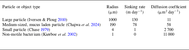


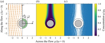


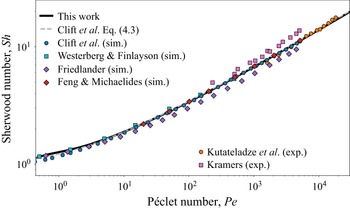


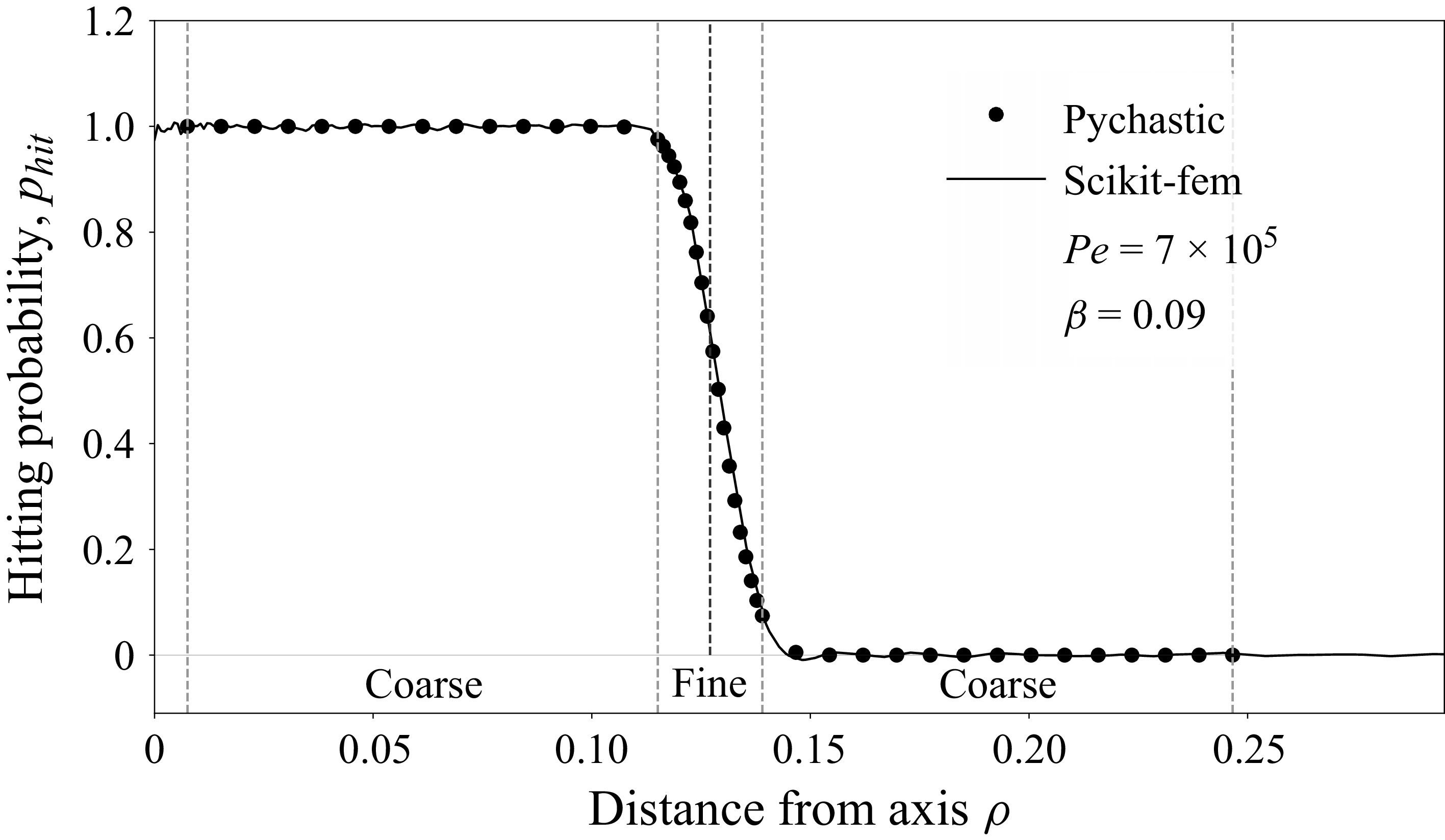


 Open access

