





1. Introduction
Structures in tokamak plasmas are anisotropic: they are elongated along the field line but short perpendicular to it. Many tokamak simulation codes, especially core codes such as GS2 (Dorland et al. Reference Dorland, Jenko, Kotschenreuther and Rogers2000; Barnes et al. Reference Barnes2024), GENE (Jenko et al. Reference Jenko, Dorland, Kotschenreuther and Rogers2000; Görler et al. Reference Görler, Lapillonne, Brunner, Dannert, Jenko, Merz and Told2011) and GYRO (Candy Reference Candy2009; Candy & Belli Reference Candy and Belli2010), take advantage of this by using a field-aligned coordinate system; the field-aligned coordinate system allows for coarse resolution along the field line reducing computational expense (Beer, Cowley & Hammett Reference Beer, Cowley and Hammett1995). However, field-aligned coordinate systems have a coordinate singularity at magnetic X-points where the poloidal magnetic field vanishes, so using field-aligned coordinate systems in edge codes which simulate a portion of the core and scrape-off layer (SOL) simultaneously is more difficult (Stegmeir et al. Reference Stegmeir, Coster, Maj, Hallatschek and Lackner2016; Leddy et al. Reference Leddy, Dudson, Romanelli, Shanahan and Walkden2017). Grids using field-aligned coordinates also suffer from cell deformation in the presence of strong magnetic shear which can be addressed using the shifted metric procedure (Scott Reference Scott1998, Reference Scott2001; Dimits Reference Dimits1993).
There have been a variety of approaches to handling the coordinate singularity at the X-point. BOUT++ handles it by using multiple blocks, each with a field-aligned coordinate system, and avoiding the calculation of geometric quantities at the X-point (Leddy et al. Reference Leddy, Dudson, Romanelli, Shanahan and Walkden2017; Dudson et al. Reference Dudson, Kryjak, Muhammed, Hill and Omotani2024). Flux-aligned coordinates do not suffer from the same shear as field-aligned coordinates since they typically use the toroidal angle as a coordinate, but they are also singular at X-points. This singularity can be cured numerically (Mattor Reference Mattor1995), but still have resolution imbalances near the X-point. COGENT uses multiple blocks each with a coordinate system that is flux aligned except near the X-point where they overlap. A high-order interpolation scheme is used to transfer information between the overlapping regions of each block (McCorquodale et al. Reference McCorquodale, Dorr, Hittinger and Colella2015; Dorf et al. Reference Dorf, Dorr, Hittinger, Cohen and Rognlien2016). The two-dimensional (2-D) fluid codes SOLPS (Wiesen et al. Reference Wiesen2015) and UEDGE (Rognlien et al. Reference Rognlien, Milovich, Rensink and Porter1992) as well as the 3-D fluid code SOLEDGE3X (Bufferand et al. Reference Bufferand2024) also employ flux-aligned coordinates.
Other edge gyrokinetic codes such as GENE-X (Michels et al. Reference Michels, Stegmeir, Ulbl, Jarema and Jenko2021) and fluid codes such as GRILLIX (Stegmeir et al. Reference Stegmeir, Finkbeiner, Pitzal, Geiger and Jenko2026), which use the same framework (Stegmeir et al. Reference Stegmeir, Coster, Maj, Hallatschek and Lackner2016), have abandoned field- and flux-aligned coordinates in favour of the flux-coordinate-independent (FCI) approach because of the difficulty of dealing with the singularity at the X-point. The gyro-fluid code FELTOR (Wiesenberger & Held Reference Wiesenberger and Held2024) uses a discontinuous Galerkin formulation of the FCI approach (Wiesenberger & Held Reference Wiesenberger and Held2023). The FCI approach breaks the simulation domain into a series of poloidal planes which do not have a field-aligned coordinate system and employs a field-line-following discretisation of the parallel derivative operator to minimise the number of poloidal planes needed. Interpolation within the poloidal plane is required to compute the parallel derivatives (Hariri & Ottaviani Reference Hariri and Ottaviani2013; Stegmeir et al. Reference Stegmeir, Coster, Maj, Hallatschek and Lackner2016, Reference Stegmeir, Coster, Ross, Maj, Lackner and Poli2018). Another alternative is to forego the resolution advantages offered by FCI and field-aligned coordinate systems and use a cylindrical coordinate system as is done in the fluid code GBS (Giacomin et al. Reference Giacomin, Ricci, Coroado, Fourestey, Galassi, Lanti, Mancini, Richart, Stenger and Varini2022).
Here, we present an algorithm for grid generation and computing geometric quantities in a standard field-aligned coordinate system that avoids the singularity at the X-point. We employ a multi-block approach where each block conforms to the separatrix leaving no gap around the X-point. Our numerical scheme allows us to avoid calculation of any geometric quantities or fluxes at the X-point while still having block corners at the X-point. We implement and test this algorithm in the gyrokinetic model in the Gkeyll simulation framework (Hakim et al. Reference Hakim, Hammett, Shi and Mandell2019; Mandell et al. Reference Mandell, Hakim, Hammett and Francisquez2020; Shukla et al. Reference Shukla, Roeltgen, Kotschenreuther, Juno, Bernard, Hakim, Hammett, Hatch, Mahajan and Francisquez2025b ; Francisquez et al. Reference Francisquez, Cagas, Shukla, Juno and Hammett2026). Consistent with findings in Wiesenberger et al. (Reference Wiesenberger, Held, Einkemmer and Kendl2018), we find that convergence is reduced in the vicinity of the X-point.
The rest of the paper is organised as follows: in § 2 we give background on the Clebsch representation of magnetic fields and field-aligned coordinates, in § 3 we present the equations of our gyrokinetic model in a field-aligned coordinate system, in § 4 we detail the coordinate system we employ, in § 5 we show how the spatial discretisation of our algorithm avoids the coordinate singularity at the X-point and in § 6 we describe how we generate simulation grids and calculate geometric quantities and also show example grids. Finally, in § 7, we conduct convergence and consistency tests and show an example 2-D axisymmetric gyrokinetic simulation of the spherical tokamak for energy production (STEP) (Karhunen et al. Reference Karhunen, Henderson, Järvinen, Moulton, Newton and Osawa2024) using our algorithm. Although we find that convergence is reduced in the vicinity of the X-point, our scheme converges faster than first order for all tests and maintains exact particle conservation even in domains with an X-point.
2. Coordinate systems for magnetised plasma simulations
As is well known, in certain situations (described below), we can write the magnetic field in the Clebsch representation (Dhaeseleer et al. Reference Dhaeseleer, Hitchon, Shohet, Callen and Kerst1991)
 \begin{align} \boldsymbol{B} = \boldsymbol{\nabla }\psi \times \boldsymbol{\nabla }\alpha , \end{align}
where $\psi (\boldsymbol{x})$
and
$\psi (\boldsymbol{x})$
and $\alpha (\boldsymbol{x})$
are scalar functions of the position vector
$\alpha (\boldsymbol{x})$
are scalar functions of the position vector $\boldsymbol{x}$
. However, not all magnetic field configurations can be described by the Clebsch representation: the field lines of Clebsch-representable magnetic fields are integrable and hence enforce some stringent constraints on the type of fields that can be described in this way.Footnote
1
Thankfully, for tokamaks, where the fields are axisymmetric, or in regions of stellarators with nested flux surfaces, such representations can be found. Hence, in this paper we will restrict ourselves to such magnetic configurations.
$\boldsymbol{x}$
. However, not all magnetic field configurations can be described by the Clebsch representation: the field lines of Clebsch-representable magnetic fields are integrable and hence enforce some stringent constraints on the type of fields that can be described in this way.Footnote
1
Thankfully, for tokamaks, where the fields are axisymmetric, or in regions of stellarators with nested flux surfaces, such representations can be found. Hence, in this paper we will restrict ourselves to such magnetic configurations.
The importance of the Clebsch representation (when it exists) is that the two vectors $\boldsymbol{\nabla }\psi$
and
$\boldsymbol{\nabla }\psi$
and $\boldsymbol{\nabla }\alpha$
can be used as the dual basis vectors (contravariant basis) of a field-line-following coordinate system. To understand what this means and establish notation for rest of the paper consider an arbitrary coordinate transform given by the invertible map
$\boldsymbol{\nabla }\alpha$
can be used as the dual basis vectors (contravariant basis) of a field-line-following coordinate system. To understand what this means and establish notation for rest of the paper consider an arbitrary coordinate transform given by the invertible map
 \begin{align} \boldsymbol{x} = \boldsymbol{x}(z^1, z^2, z^3) , \end{align}
where $(z^1, z^2, z^3)$
are computational coordinates. This maps a rectangular region in
$(z^1, z^2, z^3)$
are computational coordinates. This maps a rectangular region in $\mathbb{R}^3$
to a (generally non-rectangular) region of physical space. Once this mapping is known then we can compute the tangent vectors
$\mathbb{R}^3$
to a (generally non-rectangular) region of physical space. Once this mapping is known then we can compute the tangent vectors
 \begin{align} \boldsymbol{e}_{i} = \frac {\partial \boldsymbol{x}}{\partial z^i} \end{align}
and the dual vectors $\boldsymbol{e}^{i}$
defined implicitly by the relation
$\boldsymbol{e}^{i}$
defined implicitly by the relation
 \begin{align} \boldsymbol{e}^{i}\boldsymbol{\cdot }\boldsymbol{e}_{j} = \delta {^i_j}. \end{align}
If the inverse mapping $z^i = z^i(\boldsymbol{x})$
is known, then we can show that
$z^i = z^i(\boldsymbol{x})$
is known, then we can show that $\boldsymbol{e}^{i} = \boldsymbol{\nabla }z^i$
. At each point
$\boldsymbol{e}^{i} = \boldsymbol{\nabla }z^i$
. At each point $\boldsymbol{x}$
either the tangents or duals form a linearly independent set of vectors and hence can be used to represent vector and tensor quantities at that point. For example, a vector
$\boldsymbol{x}$
either the tangents or duals form a linearly independent set of vectors and hence can be used to represent vector and tensor quantities at that point. For example, a vector $\boldsymbol{a}$
can be written as
$\boldsymbol{a}$
can be written as
 \begin{align} \boldsymbol{a} = a^i \boldsymbol{e}_{i} = a_i \boldsymbol{e}^{i} , \end{align}
where $a^i = \boldsymbol{a}\boldsymbol{\cdot }\boldsymbol{e}^{i}$
,
$a^i = \boldsymbol{a}\boldsymbol{\cdot }\boldsymbol{e}^{i}$
, $a_i = \boldsymbol{a}\boldsymbol{\cdot }\boldsymbol{e}_{i}$
and we have assumed the summation convention over repeated indices. Once the tangent and dual vectors are determined we can compute the covariant and contravariant components of the metric tensor as
$a_i = \boldsymbol{a}\boldsymbol{\cdot }\boldsymbol{e}_{i}$
and we have assumed the summation convention over repeated indices. Once the tangent and dual vectors are determined we can compute the covariant and contravariant components of the metric tensor as
 \begin{align} g_{ij} &= \boldsymbol{e}_{i}\boldsymbol{\cdot }\boldsymbol{e}_{j} ,\\[-10pt]\nonumber\end{align}
 \begin{align} g^{ij} &= \boldsymbol{e}^{i}\boldsymbol{\cdot }\boldsymbol{e}^{j}. \end{align}
Defining the Jacobian (volume element) of the transform $J_c = \boldsymbol{e}_{1}\boldsymbol{\cdot }(\boldsymbol{e}_{2}\times \boldsymbol{e}_{3})$
we can easily derive the explicit expressions for the duals
$J_c = \boldsymbol{e}_{1}\boldsymbol{\cdot }(\boldsymbol{e}_{2}\times \boldsymbol{e}_{3})$
we can easily derive the explicit expressions for the duals
 \begin{align} \boldsymbol{e}^{1} &= \frac {1}{J_c} \boldsymbol{e}_{2}\times \boldsymbol{e}_{3} ,\\[-10pt]\nonumber\end{align}
 \begin{align} \boldsymbol{e}^{2} &= \frac {1}{J_c} \boldsymbol{e}_{3}\times \boldsymbol{e}_{1} ,\\[-10pt]\nonumber\end{align}
 \begin{align} \boldsymbol{e}^{3} &= \frac {1}{J_c} \boldsymbol{e}_{1}\times \boldsymbol{e}_{2}. \end{align}
From this we also see that $J_c^{-1} = \boldsymbol{e}^{1}\boldsymbol{\cdot }(\boldsymbol{e}^{2}\times \boldsymbol{e}^{3}) = \boldsymbol{\nabla }z^1\boldsymbol{\cdot }(\boldsymbol{\nabla }z^2\times \boldsymbol{\nabla }z^3)$
. We assume that the bases are arranged such that
$J_c^{-1} = \boldsymbol{e}^{1}\boldsymbol{\cdot }(\boldsymbol{e}^{2}\times \boldsymbol{e}^{3}) = \boldsymbol{\nabla }z^1\boldsymbol{\cdot }(\boldsymbol{\nabla }z^2\times \boldsymbol{\nabla }z^3)$
. We assume that the bases are arranged such that $J_c \gt 0$
.
$J_c \gt 0$
.
As we need the mapping to be invertible we must ensure that $J_c(\boldsymbol{x})$
does not vanish anywhere in the domain. At the
$J_c(\boldsymbol{x})$
does not vanish anywhere in the domain. At the $X$
- and
$X$
- and $O$
-points of a tokamak configurations, however, we have
$O$
-points of a tokamak configurations, however, we have $J_c = 0$
for field-line-following coordinates, that is, the coordinate system is non-invertible. We get around this issue by ensuring that we do not compute any geometrical quantities or numerical fluxes at these isolated singular points in the domain. The use of a high-order scheme (we use the discontinuous Galerkin scheme) that uses interior (to surfaces and volumes) quadrature nodes where numerical fluxes are computed, automatically ensures this, allowing us to work with coordinate systems that have singularities at a finite set of isolated points. However, despite not computing any geometric or physical quantity at the
$J_c = 0$
for field-line-following coordinates, that is, the coordinate system is non-invertible. We get around this issue by ensuring that we do not compute any geometrical quantities or numerical fluxes at these isolated singular points in the domain. The use of a high-order scheme (we use the discontinuous Galerkin scheme) that uses interior (to surfaces and volumes) quadrature nodes where numerical fluxes are computed, automatically ensures this, allowing us to work with coordinate systems that have singularities at a finite set of isolated points. However, despite not computing any geometric or physical quantity at the $X$
- or
$X$
- or $O$
-points, we ensure a corner node lies exactly there, producing an accurate representation of the geometry, without any ‘holes’. As will be discussed in § 7, avoiding evaluation at the X-point does not entirely remove the effect of the coordinate singularity.
$O$
-points, we ensure a corner node lies exactly there, producing an accurate representation of the geometry, without any ‘holes’. As will be discussed in § 7, avoiding evaluation at the X-point does not entirely remove the effect of the coordinate singularity.
Identifying the dual vectors as $\boldsymbol{e}^{i} = \boldsymbol{\nabla }z^i$
, we can see why the Clebsch form (2.1) is useful: once we find the Clebsch form we can construct a coordinate system (as described later in this paper) such that the resulting mapping has
$\boldsymbol{e}^{i} = \boldsymbol{\nabla }z^i$
, we can see why the Clebsch form (2.1) is useful: once we find the Clebsch form we can construct a coordinate system (as described later in this paper) such that the resulting mapping has $\boldsymbol{e}^{1} = \boldsymbol{\nabla }\psi$
and
$\boldsymbol{e}^{1} = \boldsymbol{\nabla }\psi$
and $\boldsymbol{e}^{2} = \boldsymbol{\nabla }\alpha$
. With this, the two scalar function
$\boldsymbol{e}^{2} = \boldsymbol{\nabla }\alpha$
. With this, the two scalar function $z^1 = \psi$
and
$z^1 = \psi$
and $z^2 = \alpha$
would be two of the three computational coordinates. The choice of the third coordinate,
$z^2 = \alpha$
would be two of the three computational coordinates. The choice of the third coordinate, $z^3 = \theta$
, called the field-line coordinate, can then be made independently.
$z^3 = \theta$
, called the field-line coordinate, can then be made independently.
Now, as $\boldsymbol{B} = \boldsymbol{\nabla }\psi \times \boldsymbol{\nabla }\alpha = \boldsymbol{e}^{1}\times \boldsymbol{e}^{2}$
we must have
$\boldsymbol{B} = \boldsymbol{\nabla }\psi \times \boldsymbol{\nabla }\alpha = \boldsymbol{e}^{1}\times \boldsymbol{e}^{2}$
we must have
 \begin{align} \boldsymbol{B}\boldsymbol{\cdot }\boldsymbol{e}^{1} = \boldsymbol{B}\boldsymbol{\cdot }\boldsymbol{e}^{2} = 0 , \end{align}
and hence
 \begin{align} \boldsymbol{B} = (\boldsymbol{B}\boldsymbol{\cdot }\boldsymbol{e}^{3})\boldsymbol{e}_{3} = \frac {1}{J_c} \boldsymbol{e}_{3}. \end{align}
From this we get a relation between the Jacobian, the magnitude of the magnetic field and the $g_{33}$
 \begin{align} J_c B = \sqrt {g_{33}}. \end{align}
In these field-line-following coordinates the magnetic field always points in the direction of $\boldsymbol{e}_{3}$
. The unit vector in the direction of the magnetic field is
$\boldsymbol{e}_{3}$
. The unit vector in the direction of the magnetic field is
 \begin{align} \boldsymbol{b} = \frac {\boldsymbol{e}_{3}}{\| \boldsymbol{e}_{3} \|} . \end{align}
The choice of these field-line-following coordinates, is not, in general, global or unique, and depends on the topologically distinct regions that need to be included in a simulation. In general, a single mapping is not usually enough to cover all of the physical region of interest, and hence several maps are needed that between them cover the physical domain (Leddy et al. Reference Leddy, Dudson, Romanelli, Shanahan and Walkden2017; Bufferand et al. Reference Bufferand2024). For simple devices, like the magnetic mirror, a single coordinate map is enough to grid the complete domain. However, for tokamaks we usually have to divide the physical domain into multiple regions, at least one for each topologically distinct region, and construct field-line-following coordinates specific to each region. For example, for a double-null configuration we have to construct separate coordinate systems in the outer and inner SOLs, the upper and lower private flux (PF) regions and the core region. In our implementation, in fact, for double-null configurations, we generate five maps to ensure a reasonably smooth grid that includes the core, the SOLs and the PF regions. We refer to the assembly of grids that covers the entire physical region of interest as a multi-block grid.
3. Transforms of the gyrokinetic equation
3.1. The gyrokinetic equations
The electrostatic gyrokinetic equation can be written as a Hamiltonian system
 \begin{align} \frac {\partial f}{\partial t} + \{f,H\} = 0 , \end{align}
where $f$
is the distribution function and
$f$
is the distribution function and $H$
is the Hamiltonian. In conservative form we can write this as
$H$
is the Hamiltonian. In conservative form we can write this as
 \begin{align} \frac {\partial (\mathcal{J}f)}{\partial t} + \boldsymbol{\nabla} _{\boldsymbol{x}}\boldsymbol{\cdot }(\mathcal{J}\dot {\boldsymbol{x}} f) + \frac {\partial }{\partial v_\parallel } (\mathcal{J}\dot {v}_\parallel f) = 0 , \end{align}
where $v_\parallel$
is the velocity parallel to the magnetic field,
$v_\parallel$
is the velocity parallel to the magnetic field, $\mu$
is the magnetic moment,
$\mu$
is the magnetic moment, $\dot {\boldsymbol{x}} = \{\boldsymbol{x},H\}$
,
$\dot {\boldsymbol{x}} = \{\boldsymbol{x},H\}$
, $\dot {v}_\parallel = \{v_\parallel ,H\}$
and
$\dot {v}_\parallel = \{v_\parallel ,H\}$
and $\mathcal{J} = B_\parallel ^*/m$
. Further, for any two phase-space functions
$\mathcal{J} = B_\parallel ^*/m$
. Further, for any two phase-space functions $f(\boldsymbol{x},v_\parallel ,\mu )$
and
$f(\boldsymbol{x},v_\parallel ,\mu )$
and $g(\boldsymbol{x},v_\parallel ,\mu )$
the Poisson bracket is given by
$g(\boldsymbol{x},v_\parallel ,\mu )$
the Poisson bracket is given by
 \begin{align} \{f,g\} = \frac {\boldsymbol{B}^*}{m B_\parallel ^*} \boldsymbol{\cdot }\left ( \boldsymbol{\nabla} _{\boldsymbol{x}} f \frac {\partial g}{\partial v_\parallel } - \frac {\partial f}{\partial v_\parallel } \boldsymbol{\nabla} _{\boldsymbol{x}} g \right ) - \frac {\boldsymbol{b}}{q B_\parallel ^*} \times \boldsymbol{\nabla} _{\boldsymbol{x}} f \boldsymbol{\cdot }\boldsymbol{\nabla} _{\boldsymbol{x}} g , \end{align}
where $\boldsymbol{B}^* = \boldsymbol{B} + (m v_\parallel /q) \boldsymbol{\nabla} _{\boldsymbol{x}}\times \boldsymbol{b}$
and
$\boldsymbol{B}^* = \boldsymbol{B} + (m v_\parallel /q) \boldsymbol{\nabla} _{\boldsymbol{x}}\times \boldsymbol{b}$
and $B_\parallel ^* = \boldsymbol{b}\boldsymbol{\cdot }\boldsymbol{B}^* \approx B$
. The gyrocentre Hamiltonian is
$B_\parallel ^* = \boldsymbol{b}\boldsymbol{\cdot }\boldsymbol{B}^* \approx B$
. The gyrocentre Hamiltonian is
 \begin{align} H = \frac {1}{2} m v_\parallel ^2 + \mu B + q \phi , \end{align}
where $m$
is the species’ mass,
$m$
is the species’ mass, $q$
is the species’ charge and
$q$
is the species’ charge and $\phi$
is the electrostatic potential. Here, we have taken the long-wavelength (drift-kinetic) limit to neglect gyroaveraging of
$\phi$
is the electrostatic potential. Here, we have taken the long-wavelength (drift-kinetic) limit to neglect gyroaveraging of $\phi$
(Mandell et al. Reference Mandell, Hakim, Hammett and Francisquez2020). Substituting the Hamiltonian into the Poisson bracket, we get
$\phi$
(Mandell et al. Reference Mandell, Hakim, Hammett and Francisquez2020). Substituting the Hamiltonian into the Poisson bracket, we get
 \begin{align} \{f,H\} &= \frac {\boldsymbol{B}^*}{m B_\parallel ^*} \boldsymbol{\cdot }\left ( m v_\parallel \boldsymbol{\nabla} _{\boldsymbol{x}} f - \frac {\partial f}{\partial v_\parallel } \boldsymbol{\nabla} _{\boldsymbol{x}} H \right ) - \frac {\boldsymbol{b}}{q B_\parallel ^*} \times \boldsymbol{\nabla} _{\boldsymbol{x}} f \boldsymbol{\cdot }\boldsymbol{\nabla} _{\boldsymbol{x}} H ,\end{align}
where
 \begin{align} \boldsymbol{\nabla} _{\boldsymbol{x}} H = \mu \boldsymbol{\nabla} _{\boldsymbol{x}} B + q\boldsymbol{\nabla} _{\boldsymbol{x}}\phi . \end{align}
The characteristics are
 \begin{align} \dot {\boldsymbol{x}} = \{\boldsymbol{x},H\} = \frac {\boldsymbol{B}^*}{B_\parallel ^*} v_\parallel + \frac {\boldsymbol{b}}{q B_\parallel ^*} \times \boldsymbol{\nabla} _{\boldsymbol{x}} H , \end{align}
and
 \begin{align} \dot {v}_\parallel = \{{v}_\parallel ,H\} = -\frac {\boldsymbol{B}^*}{m B_\parallel ^*}\boldsymbol{\cdot }\boldsymbol{\nabla} _{\boldsymbol{x}} H. \end{align}
The electrostatic potential $\phi$
is determined by the gyrokinetic Poisson equation (also sometimes called the quasineutrality equation)
$\phi$
is determined by the gyrokinetic Poisson equation (also sometimes called the quasineutrality equation)
 \begin{align} -\boldsymbol{\nabla} _{\boldsymbol{x}}\boldsymbol{\cdot }\left ( \varepsilon _\perp \boldsymbol{\nabla} _\perp \phi \right ) = \sum _s q_s \int \mathcal{J} f_s \thinspace \text{d}^3\boldsymbol{v} , \end{align}
where $\varepsilon _\perp (\boldsymbol{x})$
is a polarisation tensor and
$\varepsilon _\perp (\boldsymbol{x})$
is a polarisation tensor and $\text{d}^3\boldsymbol v = \text{d}\mu \text{d}v_\parallel$
indicates integration of velocity space. The operator
$\text{d}^3\boldsymbol v = \text{d}\mu \text{d}v_\parallel$
indicates integration of velocity space. The operator $\boldsymbol{\nabla} _\perp$
is defined as
$\boldsymbol{\nabla} _\perp$
is defined as
 \begin{align} \boldsymbol{\nabla} _\perp = \boldsymbol{\nabla} _{\boldsymbol{x}} - \boldsymbol{b}(\boldsymbol{b}\boldsymbol{\cdot }\boldsymbol{\nabla} _{\boldsymbol{x}}). \end{align}
Even in the long-wavelength limit with no gyroaveraging, the first-order polarisation charge density on the left-hand side of (3.9) incorporates some finite-Larmor-radius effects (Mandell et al. Reference Mandell, Hakim, Hammett and Francisquez2020). Note that, as will be discussed later in § 3.2, the flute ordering approximation ( $k_\parallel \ll k_\perp )$
can be employed to drop derivatives parallel to the magnetic field in the gyrokinetic Poisson equation.
$k_\parallel \ll k_\perp )$
can be employed to drop derivatives parallel to the magnetic field in the gyrokinetic Poisson equation.
Until this point we have written all equations in a coordinate-independent form. Now we introduce coordinates. Consider transforming the configuration space coordinates as
 \begin{align} \boldsymbol{x} = \boldsymbol{x}(z^1,z^2,z^3) , \end{align}
where $(z^1,z^2,z^3)$
are computational coordinates. From this mapping, as we discussed above, we can compute the tangent vectors, the duals and the co- and contravariant components of the metric tensor.
$(z^1,z^2,z^3)$
are computational coordinates. From this mapping, as we discussed above, we can compute the tangent vectors, the duals and the co- and contravariant components of the metric tensor.
One we have the tangents and duals, we can construct the fundamental vector derivative operator
 \begin{align} \boldsymbol{\nabla} _{\boldsymbol{x}} = \boldsymbol{e}^{i}\frac {\partial }{\partial z^i}. \end{align}
This operator is enough now to write the equations in arbitrary coordinate systems. To ease the derivations we need the identities
 \begin{align} \boldsymbol{\nabla} _{\boldsymbol{x}}\boldsymbol{\cdot }\boldsymbol{U} = \frac {1}{J_c}\frac {\partial }{\partial z^i}\left (J_c \boldsymbol{e}^{i}\boldsymbol{\cdot }\boldsymbol{U} \right ) \end{align}
and
 \begin{align} \boldsymbol{\nabla} _{\boldsymbol{x}}\times \boldsymbol{U} &= \frac {1}{J_c}\frac {\partial }{\partial z^i} \left ( \epsilon ^{ijk} U_j \right ) \boldsymbol{e}_{k}\\[-10pt]\nonumber \end{align}
 \begin{align} &= \frac {1}{J_c}\left ( \frac {\partial U_3}{\partial z^2} - \frac {\partial U_2}{\partial z^3} \right ) \boldsymbol{e}_{1} + \frac {1}{J_c}\left ( \frac {\partial U_1}{\partial z^3} - \frac {\partial U_3}{\partial z^1} \right ) \boldsymbol{e}_{2} + \frac {1}{J_c}\left ( \frac {\partial U_2}{\partial z^1} - \frac {\partial U_1}{\partial z^2} \right ) \boldsymbol{e}_{3} ,\end{align}
where $\boldsymbol{U}$
is any vector field and
$\boldsymbol{U}$
is any vector field and $\epsilon ^{ijk}$
is the Levi-Civita tensor.
$\epsilon ^{ijk}$
is the Levi-Civita tensor.
3.2. Gyrokinetic equation in field-aligned coordinates
The gyrokinetic equation in computational coordinates becomes
 \begin{align} \frac {\partial (\mathcal{J}J_cf)}{\partial t} + \frac {\partial }{\partial z^i} ( \mathcal{J}J_c(\boldsymbol{e}^{i}\boldsymbol{\cdot }\dot {\boldsymbol{x}}) f ) + \frac {\partial }{\partial v_\parallel } (\mathcal{J}J_c\dot {v}_\parallel f) = 0. \end{align}
Further, in these coordinates we have
 \begin{align} \boldsymbol{B}^* = (\boldsymbol{B}\boldsymbol{\cdot }\boldsymbol{e}^{3})\boldsymbol{e}_{3} + \frac {m v_\parallel }{q} \frac {1}{J_c} \frac {\partial }{\partial z^i} ( \epsilon ^{ijk} b_j ) \boldsymbol{e}_{k} , \end{align}
where $b_j = \boldsymbol{e}_{j}\boldsymbol{\cdot }\boldsymbol{b}$
. Hence, we have
$b_j = \boldsymbol{e}_{j}\boldsymbol{\cdot }\boldsymbol{b}$
. Hence, we have
 \begin{align} \boldsymbol{e}^{i}\boldsymbol{\cdot }\boldsymbol{B}^* = (\boldsymbol{B}\boldsymbol{\cdot }\boldsymbol{e}^{3})\delta {^i_3} + \frac {m v_\parallel }{q} \frac {1}{J_c} \frac {\partial }{\partial z^k} ( \epsilon ^{kji} b_j ). \end{align}
Further, we can compute
 \begin{align} \boldsymbol{e}^{i}\boldsymbol{\cdot }(\boldsymbol{b}\times \boldsymbol{\nabla} _{\boldsymbol{x}} H) = \boldsymbol{e}^{i}\boldsymbol{\cdot }(\boldsymbol{e}^{j}\times \boldsymbol{e}^{k}) b_j \frac {\partial H}{\partial z^k} = \frac {\epsilon ^{ijk}}{J_c} b_j \frac {\partial H}{\partial z^k}. \end{align}
Hence, we have
 \begin{align} \boldsymbol{e}^{i}\boldsymbol{\cdot }\dot {\boldsymbol{x}} = \frac {v_\parallel }{B^*_\parallel } (\boldsymbol{e}^{i}\boldsymbol{\cdot }\boldsymbol{B}^*) + \frac {1}{q B^*_\parallel } \frac {\epsilon ^{ijk}}{J_c} b_j \frac {\partial H}{\partial z^k}. \end{align}
Further, we have
 \begin{align} \dot {v}_\parallel = -\frac {(\boldsymbol{e}^{k}\boldsymbol{\cdot }\boldsymbol{B}^*)}{m B_\parallel ^*}\frac {\partial H}{\partial z^k}. \end{align}
We can again use (3.18) to compute $\boldsymbol{e}^{k}\boldsymbol{\cdot }\boldsymbol{B}^*$
.
$\boldsymbol{e}^{k}\boldsymbol{\cdot }\boldsymbol{B}^*$
.
The gyrokinetic Poisson equation in computational coordinates becomes
 \begin{align} -\frac {1}{J_c} \frac {\partial }{\partial z^i} \left ( J_c \varepsilon _\perp \boldsymbol{e}^{i}\boldsymbol{\cdot }\boldsymbol{\nabla} _\perp \phi \right ) = \sum _s q_s \int \mathcal{J} f_s \thinspace \text{d}^3\boldsymbol{v}. \end{align}
We can compute
 \begin{align} \boldsymbol{e}^{i}\boldsymbol{\cdot }\boldsymbol{\nabla} _\perp \phi &= \boldsymbol{e}^{i}\boldsymbol{\cdot }\boldsymbol{e}^{j}\frac {\partial \phi }{\partial z^j} - (\boldsymbol{e}^{i}\boldsymbol{\cdot }\boldsymbol{b}) (\boldsymbol{b}\boldsymbol{\cdot }\boldsymbol{e}^{m})\frac {\partial \phi }{\partial z^m}\\[-10pt]\nonumber \end{align}
 \begin{align} &= g^{ij} \frac {\partial \phi }{\partial z^j} - \delta {^i_3}\frac {1}{\lVert \boldsymbol{e}_{3} \rVert ^2 } \frac {\partial \phi }{\partial z^3}. \end{align}
Note that in gyrokinetics we typically drop the derivatives in $z^3$
in the gyrokinetic Poisson equation due to the assumption that gradient scale lengths in the parallel direction are much longer than those in the perpendicular direction. This is the commonly used ‘flute approximation’ (Scott Reference Scott2010; Seto et al. Reference Seto, Xu, Dudson and Yagi2019). Also note that, while this ordering is a good approximation for high-n (toroidal mode number) modes, it can lead to inaccurate solutions for low-n modes, in particular n = 0 modes, near the X-point (Dudson & Leddy Reference Dudson and Leddy2017; Seto et al. Reference Seto, Dudson, Xu and Yagi2023).
$z^3$
in the gyrokinetic Poisson equation due to the assumption that gradient scale lengths in the parallel direction are much longer than those in the perpendicular direction. This is the commonly used ‘flute approximation’ (Scott Reference Scott2010; Seto et al. Reference Seto, Xu, Dudson and Yagi2019). Also note that, while this ordering is a good approximation for high-n (toroidal mode number) modes, it can lead to inaccurate solutions for low-n modes, in particular n = 0 modes, near the X-point (Dudson & Leddy Reference Dudson and Leddy2017; Seto et al. Reference Seto, Dudson, Xu and Yagi2023).
3.3. Simplifications in axisymmetric limit
For divertor design, axisymmetric simulations which are two-dimensional rather than three-dimensional in configuration space are often used (Dominski et al. Reference Dominski, Maget, Manas, Morales, Ku, Scheinberg, Chang, Hager and O’Mullane2024; Shukla et al. Reference Shukla, Roeltgen, Kotschenreuther, Hatch, Francisquez, Juno, Bernard, Hakim, Hammett and Mahajan2025a
,
Reference Shukla, Roeltgen, Kotschenreuther, Juno, Bernard, Hakim, Hammett, Hatch, Mahajan and Francisquezb
). In these simulations, cross-field transport is modelled with ad hoc diffusive terms. If we take the second computational coordinate $z^2$
as our ignorable coordinate assuming
$z^2$
as our ignorable coordinate assuming $\partial F/\partial z^2 = 0$
for all quantities
$\partial F/\partial z^2 = 0$
for all quantities $F$
, we get the following equations of motion by taking
$F$
, we get the following equations of motion by taking $i=1,3$
in (3.20):
$i=1,3$
in (3.20):
 \begin{equation} \boldsymbol e^1 \boldsymbol{\cdot }\boldsymbol{\dot x} = \dot z^1 = -\frac {mv_\parallel ^2}{qJ_cB^*_\parallel }\frac {\partial b_2}{\partial z^3} + \frac {b_2}{qJ_cB_\parallel ^*} \frac {\partial H}{\partial z^3} , \end{equation}
 \begin{align} \boldsymbol e^3 \boldsymbol{\cdot }\boldsymbol{\dot x} = \dot z^3 = \frac {Cv_\parallel }{J_cB_\parallel ^*} + \frac {mv_\parallel ^2}{qJ_cB^*_\parallel }\frac {\partial b_2}{\partial z^1} + \frac {b_2}{qJ_cB_\parallel ^*} \frac {\partial H}{\partial z^1} \end{align}
and (3.21)
 \begin{align} \dot v_\parallel = -\frac {C}{mJ_cB_\parallel ^*}\frac {\partial H}{\partial z^3} + \frac {v_\parallel }{qJ_cB_\parallel ^*} \left (\frac {\partial b_2}{\partial z^3}\frac {\partial H}{\partial z^1} - \frac {\partial b_2}{z^1}\frac {\partial H}{\partial z^3}\right ) . \end{align}
Neglecting derivatives in $z^2$
in (3.22) gives the axisymmetric limit of the gyrokinetic Poisson equation. After dropping the
$z^2$
in (3.22) gives the axisymmetric limit of the gyrokinetic Poisson equation. After dropping the $z^3$
derivatives in (3.22), as is typically justified because of the long parallel and short perpendicular wavelengths present in tokamaks, neglecting derivatives in
$z^3$
derivatives in (3.22), as is typically justified because of the long parallel and short perpendicular wavelengths present in tokamaks, neglecting derivatives in $z^2$
gives the axisymmetric limit of the gyrokinetic Poisson equation
$z^2$
gives the axisymmetric limit of the gyrokinetic Poisson equation
 \begin{align} \rho = -\frac {1}{J_c} \frac {\partial }{\partial z^1} \Big [ J_c\epsilon _\perp g^{11} \frac {\partial \phi }{\partial z^1} \Big ] . \end{align}
4. Coordinate system
4.1. Coordinate definitions
Tokamak equilibrium magnetic fields are axisymmetric and can be written as (Cerfon & Freidberg Reference Cerfon and Freidberg2010)
 \begin{equation} \boldsymbol{B}=\frac {F(\psi )}{R} \boldsymbol{\hat e}_\phi +\frac {1}{R} \boldsymbol{\nabla }\psi \times \boldsymbol{\hat e}_\phi , \end{equation}
where $\boldsymbol{\hat e}_\phi$
is a unit vector and
$\boldsymbol{\hat e}_\phi$
is a unit vector and $\mu _0$
is the vacuum permeability. The poloidal flux
$\mu _0$
is the vacuum permeability. The poloidal flux $\psi$
will satisfy the Grad–Shafranov equation shown here in cylindrical
$\psi$
will satisfy the Grad–Shafranov equation shown here in cylindrical $(R,Z,\phi )$
coordinates
$(R,Z,\phi )$
coordinates
 \begin{equation} R \frac {\partial }{\partial R}\left (\frac {1}{R} \frac {\partial \psi }{\partial R}\right )+\frac {\partial ^2 \psi }{\partial Z^2}=-\mu _0 R^2 \frac {\text{d}p}{\text{d}\psi }-F \frac {\text{d}F}{\text{d}\psi } , \end{equation}
where $F$
is the poloidal current and
$F$
is the poloidal current and $p$
is the pressure. There are equilibrium codes such as the Python package FreeGS (Amorisco et al. Reference Amorisco, Agnello, Holt, Mars, Buchanan and Pamela2024; Dudson & developers Reference Dudson and developers2025), that solve (4.2) for
$p$
is the pressure. There are equilibrium codes such as the Python package FreeGS (Amorisco et al. Reference Amorisco, Agnello, Holt, Mars, Buchanan and Pamela2024; Dudson & developers Reference Dudson and developers2025), that solve (4.2) for $\psi (R,Z)$
and provide the solution in the commonly used G-formatted EQuilibrium DiSK (G-EQDSK) format Lao (Reference Lao1997).
$\psi (R,Z)$
and provide the solution in the commonly used G-formatted EQuilibrium DiSK (G-EQDSK) format Lao (Reference Lao1997).
Given $\psi (R,Z)$
we choose to use field-aligned coordinates
$\psi (R,Z)$
we choose to use field-aligned coordinates $(z^1,z^2,z^3) = (\psi ,\alpha , \theta )$
, where
$(z^1,z^2,z^3) = (\psi ,\alpha , \theta )$
, where $\alpha$
is the field-line label and
$\alpha$
is the field-line label and $\theta$
is the poloidal projection of the length along the field line normalised to
$\theta$
is the poloidal projection of the length along the field line normalised to $2\pi$
. We choose these coordinates such that our field can be represented in the Clebsch form as
$2\pi$
. We choose these coordinates such that our field can be represented in the Clebsch form as
 \begin{equation} \boldsymbol{B} = \boldsymbol{\nabla }\psi \times \boldsymbol{\nabla }\alpha . \end{equation}
Note that there are many possible choices of the parallel coordinate $\theta$
depending on the topology one wishes to represent. For example in the core of a tokamak where flux surfaces are closed, one could choose the actual poloidal angle as the parallel coordinate
$\theta$
depending on the topology one wishes to represent. For example in the core of a tokamak where flux surfaces are closed, one could choose the actual poloidal angle as the parallel coordinate $\theta$
. However, as discussed in Leddy et al. (Reference Leddy, Dudson, Romanelli, Shanahan and Walkden2017), in the SOL, the actual poloidal angle is not a suitable choice because typically more than one point on the same field would have the same value of
$\theta$
. However, as discussed in Leddy et al. (Reference Leddy, Dudson, Romanelli, Shanahan and Walkden2017), in the SOL, the actual poloidal angle is not a suitable choice because typically more than one point on the same field would have the same value of $\theta$
. (In the poloidal plane, a line of constant poloidal angle will intersect the same flux surface twice in the SOL.) For the outer SOL of a double-null tokamak configuration, the cylindrical coordinate
$\theta$
. (In the poloidal plane, a line of constant poloidal angle will intersect the same flux surface twice in the SOL.) For the outer SOL of a double-null tokamak configuration, the cylindrical coordinate $Z$
could be a suitable choice but that would of course not work for the core and would restrict the divertor plates to be horizontal in the R-Z plane which is undesirable. The choice of poloidal arc length as the parallel coordinate
$Z$
could be a suitable choice but that would of course not work for the core and would restrict the divertor plates to be horizontal in the R-Z plane which is undesirable. The choice of poloidal arc length as the parallel coordinate $\theta$
which we make here is suitable for both the open and closed field-line regions of a tokamak and allows for flexible divertor plate shapes. More details on the derivation of our coordinate system can be found in Mandell (Reference Mandell2021) and other possible choices of the parallel coordinate can be found in Jardin (Reference Jardin2010). Another similar coordinate system that aims to reduce cell deformation is described in Ribeiro & Scott (Reference Ribeiro and Scott2010).
$\theta$
which we make here is suitable for both the open and closed field-line regions of a tokamak and allows for flexible divertor plate shapes. More details on the derivation of our coordinate system can be found in Mandell (Reference Mandell2021) and other possible choices of the parallel coordinate can be found in Jardin (Reference Jardin2010). Another similar coordinate system that aims to reduce cell deformation is described in Ribeiro & Scott (Reference Ribeiro and Scott2010).
In order to have a generalised poloidal angle that sweeps out equal poloidal arc lengths, we choose the Jacobian to be
 \begin{equation} J_c =s(\psi ) \frac {R}{|\boldsymbol{\nabla }\psi |}. \end{equation}
Note here that the Jacobian is proportional to $1/|\boldsymbol{\nabla }\psi |$
. This will be true, regardless of the choice of parallel coordinate, for field-aligned coordinate systems. The coordinate singularity discussed earlier results from the fact that
$1/|\boldsymbol{\nabla }\psi |$
. This will be true, regardless of the choice of parallel coordinate, for field-aligned coordinate systems. The coordinate singularity discussed earlier results from the fact that $\boldsymbol{\nabla }\psi$
vanishes at X-points and O-points, which causes the Jacobian to diverge.
$\boldsymbol{\nabla }\psi$
vanishes at X-points and O-points, which causes the Jacobian to diverge.
With this Jacobian, the $\theta$
coordinate, parameterised in terms of the cylindrical
$\theta$
coordinate, parameterised in terms of the cylindrical $Z$
coordinate, is given by
$Z$
coordinate, is given by
 \begin{equation} \theta (R, Z)=\frac {1}{s(\psi (R, Z))} \int _{Z_{\text{lower }}(\psi )}^{Z(\psi )} \sqrt {1+\left (\frac {\partial R\left (\psi , Z^{\prime }\right )}{\partial Z^{\prime }}\right )^2} \mathrm{\,d} Z^{\prime } - \pi , \end{equation}
where the normalisation factor is
 \begin{equation} s(\psi )=\frac {1}{2 \pi } \oint \mathrm{d} \ell _p=\frac {1}{2\pi } \int _{Z_{\text{lower }}(\psi )}^{Z_{\text{upper }}(\psi )} \sqrt {1+\left (\frac {\partial R\left (\psi , Z^{\prime }\right )}{\partial Z^{\prime }}\right )^2} \mathrm{\,d} Z^{\prime } . \end{equation}
Now we define the last coordinate such that (4.3) is satisfied
 \begin{equation} \alpha (R, Z, \phi )= \phi - F(\psi ) \int _{Z_{\text{lower }}(\psi )}^{Z(\psi )} \frac {1}{|\boldsymbol{\nabla }\psi | R\left (\psi , Z^{\prime }\right )} \sqrt {1+\left (\frac {\partial R\left (\psi , Z^{\prime }\right )}{\partial Z^{\prime }}\right )^2} \mathrm{\,d} Z^{\prime } , \end{equation}
where $F(\psi ) = RB_\phi$
.
$F(\psi ) = RB_\phi$
.
The choice of computational coordinates, $(z^1, z^2, z^3) = (\psi , \alpha , \theta )$
, along with (4.6), (4.5) and (4.7), define the mapping of computational coordinates
$(z^1, z^2, z^3) = (\psi , \alpha , \theta )$
, along with (4.6), (4.5) and (4.7), define the mapping of computational coordinates $(\psi , \alpha , \theta )$
to physical
$(\psi , \alpha , \theta )$
to physical $(R,Z,\phi )$
coordinates where
$(R,Z,\phi )$
coordinates where $\theta \in [-\pi , \pi ]$
and
$\theta \in [-\pi , \pi ]$
and $\alpha \in [-\pi , \pi ]$
. From the mapping we can compute tangent vectors, dual vectors and then metric coefficients, which are written explicitly in (6.6)–(6.10).
$\alpha \in [-\pi , \pi ]$
. From the mapping we can compute tangent vectors, dual vectors and then metric coefficients, which are written explicitly in (6.6)–(6.10).
Schematic for field-line tracing in a double-null (a) and single-null (b) configurations.

The integrals in (4.5)–(4.7) are along contours of constant $\psi$
. The Z limits of the integration can be chosen based on the part of the poloidal plane one wishes to trace. For example integral in (4.6) traces from divertor plate to divertor plate in the SOL but makes a complete poloidal circuit in the core. For a double-null tokamak configuration there are 5 distinct topological regions: the outboard SOL, the inboard SOL, the lower PF region, the upper private region and the core. In figure 1(a) we show how each region is traced for a double-null tokamak. For a single-null tokamak configuration there are 3 distinct topological regions: the SOL, the PF region and the core. In figure 1(b) we show how each region is traced for a lower single-null tokamak.
$\psi$
. The Z limits of the integration can be chosen based on the part of the poloidal plane one wishes to trace. For example integral in (4.6) traces from divertor plate to divertor plate in the SOL but makes a complete poloidal circuit in the core. For a double-null tokamak configuration there are 5 distinct topological regions: the outboard SOL, the inboard SOL, the lower PF region, the upper private region and the core. In figure 1(a) we show how each region is traced for a double-null tokamak. For a single-null tokamak configuration there are 3 distinct topological regions: the SOL, the PF region and the core. In figure 1(b) we show how each region is traced for a lower single-null tokamak.
5. Discretisation of the gyrokinetic equation: avoiding the X-point
The gyrokinetic equation (3.16), for the evolution of $F = \mathcal{J} J_c f$
in the axisymmetric limit becomes
$F = \mathcal{J} J_c f$
in the axisymmetric limit becomes
 \begin{align} \frac {\partial F}{\partial t} + \dot {z}^1\frac {\partial F}{\partial z^1} + \dot {z}^3\frac {\partial F}{\partial z^3} + \dot {v_\parallel }\frac {\partial F}{\partial v_\parallel } = 0. \end{align}
We use a discontinuous Galerkin (DG) scheme to discretise this equation as described in Hakim et al. (Reference Hakim, Hammett, Shi and Mandell2019), Mandell et al. (Reference Mandell, Hakim, Hammett and Francisquez2020) and Francisquez et al. (Reference Francisquez, Cagas, Shukla, Juno and Hammett2026). The discrete approximation of $F$
in each cell
$F$
in each cell $K_i$
is given by
$K_i$
is given by
 \begin{equation} F_i=\sum _{k=1}^{N_b} F_i^{(k)} \psi _i^{(k)} , \end{equation}
where $\psi _i$
are the phase-space basis functions and
$\psi _i$
are the phase-space basis functions and $N_b$
is the number of basis functions. The discrete form of (5.1) can be obtained by projecting it onto the phase-space basis
$N_b$
is the number of basis functions. The discrete form of (5.1) can be obtained by projecting it onto the phase-space basis $\psi _j^{(k)}$
in cell
$\psi _j^{(k)}$
in cell $K_j$
and integrating by parts
$K_j$
and integrating by parts
 \begin{align} \int _{K_j} \text{d}\boldsymbol{z} \text{d}v_\parallel \text{d}\mu \psi _j^{(\ell )} \frac {\partial F}{\partial t} & +\oint _{\partial K_j} \mathrm{\,d} \boldsymbol{S}_{\mathrm{i}} \text{d}v_\parallel \text{d}\mu \psi _{j \pm }^{(\ell )} \dot {z}_{ \pm }^i \widehat {F}_{ \pm }+\oint _{\partial K_j} \text{d} \boldsymbol{z} \text{d}\mu \psi _{j \pm }^{(\ell )} \dot {v}_{\| \pm } \widehat {F_{ \pm }} \nonumber\\[4pt] & -\int _{K_j} \text{d}\boldsymbol{z} \text{d}v_\parallel \text{d}\mu \left (\frac {\partial \psi _j^{(\ell )}}{\partial z^i} \dot {z}^i+\frac {\partial \psi _j^{(\ell )}}{\partial v_\parallel } \dot {v}_{\|}\right ) F=0 , \end{align}
where $\text{d}\boldsymbol S_i$
is the surface element perpendicular to the ith direction and
$\text{d}\boldsymbol S_i$
is the surface element perpendicular to the ith direction and $\widehat {F_\pm }$
is the upwind flux evaluated at the upper and lower edges of the cell in direction i.
$\widehat {F_\pm }$
is the upwind flux evaluated at the upper and lower edges of the cell in direction i.
Substituting in the expansion of $F$
in the first term of (5.2) and making use of the orthonormality relation
$F$
in the first term of (5.2) and making use of the orthonormality relation $\int _{K_j} \text{d}\boldsymbol z \text{d}v_\parallel \text{d}\mu \psi _j^{(\ell )}\psi _j^{(k)} = \delta _{lk}$
, we get the time evolution of each expansion coefficient of
$\int _{K_j} \text{d}\boldsymbol z \text{d}v_\parallel \text{d}\mu \psi _j^{(\ell )}\psi _j^{(k)} = \delta _{lk}$
, we get the time evolution of each expansion coefficient of $F$
$F$
 \begin{align} \frac {\partial F_j^{(\ell )}}{\partial t} & +\oint _{\partial K_j} \mathrm{\,d} \boldsymbol{S}_{\mathrm{i}} \text{d}v_\parallel \text{d}\mu \psi _{j \pm }^{(\ell )} \dot {z}_{ \pm }^i \widehat {F}_{ \pm }+\oint _{\partial K_j} \text{d} \boldsymbol{z} \text{d}\mu \psi _{j \pm }^{(\ell )} \dot {v}_{\| \pm } \widehat {F_{ \pm }} \nonumber\\ & -\int _{K_j} \text{d}\boldsymbol{z} \text{d}v_\parallel \text{d}\mu \left (\frac {\partial \psi _j^{(\ell )}}{\partial z^i} \dot {z}^i+\frac {\partial \psi _j^{(\ell )}}{\partial v_\parallel } \dot {v}_{\|}\right ) F=0 . \end{align}
We evaluate the integrals in (5.4) analytically using DG expansions of the characteristics $\dot z^i$
and
$\dot z^i$
and $\dot v_\parallel$
on the phase basis in the volume term (the fourth term) and DG expansions of the fluxes (
$\dot v_\parallel$
on the phase basis in the volume term (the fourth term) and DG expansions of the fluxes ( $\dot {z}^i\hat {F}_\pm$
and
$\dot {z}^i\hat {F}_\pm$
and $\dot {v_\parallel }\hat {F}_\pm$
) in the second and third terms (the surface terms). In the last term (the volume term) the expansion of the characteristic velocities (
$\dot {v_\parallel }\hat {F}_\pm$
) in the second and third terms (the surface terms). In the last term (the volume term) the expansion of the characteristic velocities ( $\dot {z}^i$
and
$\dot {z}^i$
and $\dot {v_\parallel }$
) are constructed by evaluating the characteristics at interior Gauss–Legendre quadrature points and converting to a modal representation. In the second and third terms, the expansion of the fluxes are calculated by evaluating the flux at surface Gauss–Legendre quadrature points and converting to a modal representation. Labelling the characteristics and fluxes based on whether they are calculated by evaluation at interior or surface quadrature points with a subscripts
$\dot {v_\parallel }$
) are constructed by evaluating the characteristics at interior Gauss–Legendre quadrature points and converting to a modal representation. In the second and third terms, the expansion of the fluxes are calculated by evaluating the flux at surface Gauss–Legendre quadrature points and converting to a modal representation. Labelling the characteristics and fluxes based on whether they are calculated by evaluation at interior or surface quadrature points with a subscripts $int$
and
$int$
and $surf$
respectively, we can rewrite (5.4) as
$surf$
respectively, we can rewrite (5.4) as
 \begin{align} \frac {\partial F_j^{(\ell )}}{\partial t} & +\oint _{\partial K_j} \mathrm{\,d} \boldsymbol{S}_{\mathrm{i}} \text{d}v_\parallel \text{d}\mu \psi _{j \pm }^{(\ell )} (\dot {z}^i \widehat {F})_{\pm , surf} +\oint _{\partial K_j} \text{d} \boldsymbol{z} \text{d}\mu \psi _{j \pm }^{(\ell )} (\dot {v}_{\|} \widehat {F})_{\pm , surf} \nonumber\\[6pt] & -\int _{K_j} \text{d}\boldsymbol{z} \text{d}v_\parallel \text{d}\mu \left (\frac {\partial \psi _j^{(\ell )}}{\partial z^i} \dot {z}^i_{int}+\frac {\partial \psi _j^{(\ell )}}{\partial v_\parallel } \dot {v}_{\|,int}\right ) F=0 . \end{align}
An example of the quadrature points used in two dimensions is depicted in figure 2(a). For example, to construct the volume representation $\dot {z}^i_{int}$
in this cell, we evaluate
$\dot {z}^i_{int}$
in this cell, we evaluate $\dot z^i$
at the 4 red points and convert to a modal representation. To calculate the surface representation
$\dot z^i$
at the 4 red points and convert to a modal representation. To calculate the surface representation $(\dot z^1\hat {F})_{+,surf}$
at the upper
$(\dot z^1\hat {F})_{+,surf}$
at the upper $z^1$
edge of this cell we would evaluate
$z^1$
edge of this cell we would evaluate $\dot z^1\hat {F}$
at the two blue points at
$\dot z^1\hat {F}$
at the two blue points at $z^1=1$
and convert to a modal representation. The use of an orthonormal, modal representation for the DG fields allows us to significantly reduce the computational cost of DG (Hakim & Juno Reference Hakim and Juno2020) while respecting the need to eliminate aliasing errors in DG discretisations of kinetic equations (Juno et al. Reference Juno, Hakim, TenBarge, Shi and Dorland2018).
$z^1=1$
and convert to a modal representation. The use of an orthonormal, modal representation for the DG fields allows us to significantly reduce the computational cost of DG (Hakim & Juno Reference Hakim and Juno2020) while respecting the need to eliminate aliasing errors in DG discretisations of kinetic equations (Juno et al. Reference Juno, Hakim, TenBarge, Shi and Dorland2018).
In (a) we show the interior, surface and corner points on the unit cell. In (b) we show these points mapped to the physical domain for cells abutting the X-point. The cell in physical space is not rectangular, allowing for an accurate representation of the flux-surface geometry. The surface and interior nodes used for the evaluation of geometric quantities do not lie directly on the X-point and are thus well defined.

This method of evaluating the characteristics is the key feature of our algorithm that allows us to simulate magnetic geometries with an X-point as shown in figure 2. The geometric quantities such as the Jacobian, $J_c$
, contained in the characteristics written in (3.25)–(3.27) diverge at the X-point as mentioned below (4.4). However, since we evaluate the characteristics at either interior quadrature points or surface quadrature points and not corner points, we can avoid evaluating any geometric quantities at the X-point as long as cell corners lie at the X-point, which our multi-block grid generation routine ensures. The gyrokinetic Poisson equation, (3.22), also benefits from the distinction between corner and interior evaluations. Our solution, described in detail in Francisquez et al. (Reference Francisquez, Cagas, Shukla, Juno and Hammett2026), makes use of the interior geometric quantities to avoid the coordinate singularity. Note that while our method allows including the X-point in the domain, the effect of the coordinate singularity is not completely avoided; it affects convergence as described in § 7 and previously observed in Wiesenberger et al. (Reference Wiesenberger, Held, Einkemmer and Kendl2018).
$J_c$
, contained in the characteristics written in (3.25)–(3.27) diverge at the X-point as mentioned below (4.4). However, since we evaluate the characteristics at either interior quadrature points or surface quadrature points and not corner points, we can avoid evaluating any geometric quantities at the X-point as long as cell corners lie at the X-point, which our multi-block grid generation routine ensures. The gyrokinetic Poisson equation, (3.22), also benefits from the distinction between corner and interior evaluations. Our solution, described in detail in Francisquez et al. (Reference Francisquez, Cagas, Shukla, Juno and Hammett2026), makes use of the interior geometric quantities to avoid the coordinate singularity. Note that while our method allows including the X-point in the domain, the effect of the coordinate singularity is not completely avoided; it affects convergence as described in § 7 and previously observed in Wiesenberger et al. (Reference Wiesenberger, Held, Einkemmer and Kendl2018).
At block boundaries, one must be careful to ensure consistency; the surface normal vectors must be consistent at block boundaries. For example at a radial block boundary (the $z^1$
direction), the surface normal
$z^1$
direction), the surface normal $\boldsymbol{\hat {e}^1} = \boldsymbol{e^1}/|\boldsymbol{e_1}|$
must match. Our method for calculating the tangent vectors and metric coefficients (described in § 6.4) ensures that the surface nodes used to calculate fluxes across block boundaries are common and that the normal vectors are consistent at either side of the boundaries. Because our algorithm evolves
$\boldsymbol{\hat {e}^1} = \boldsymbol{e^1}/|\boldsymbol{e_1}|$
must match. Our method for calculating the tangent vectors and metric coefficients (described in § 6.4) ensures that the surface nodes used to calculate fluxes across block boundaries are common and that the normal vectors are consistent at either side of the boundaries. Because our algorithm evolves $F=\mathcal{J}J_cf$
rather than
$F=\mathcal{J}J_cf$
rather than $f$
, we must also be careful to correctly handle the change in the normalisation of
$f$
, we must also be careful to correctly handle the change in the normalisation of $J_c$
(4.6) at radial block boundaries. Blocks sharing a parallel boundary share the same normalisation, so there is a change only at radial block boundaries. To address this, the second term in 5.5 must be modified at radial block boundaries. The flux
$J_c$
(4.6) at radial block boundaries. Blocks sharing a parallel boundary share the same normalisation, so there is a change only at radial block boundaries. To address this, the second term in 5.5 must be modified at radial block boundaries. The flux $(\dot {z}^i\hat {F})_{\pm , surf}$
is divided by
$(\dot {z}^i\hat {F})_{\pm , surf}$
is divided by $J_c$
of the block the flux is leaving and multiplied by
$J_c$
of the block the flux is leaving and multiplied by $J_c$
of the block it is entering. The values of
$J_c$
of the block it is entering. The values of $J_c$
used for the division and multiplication are the value of
$J_c$
used for the division and multiplication are the value of $J_c$
at the surface quadrature point.
$J_c$
at the surface quadrature point.
If the normal vectors are not consistent at block boundaries or at cell boundaries, particle conservation will broken (Hakim et al. Reference Hakim, Hammett, Shi and Mandell2019). In § 7.4 we conduct a test of particle conservation which demonstrates consistency of the normal vectors and the correct handling of the re-normalisation at block boundaries.
6. Grid generation and geometric quantities
In order to conduct simulations, we need to generate a physical simulation grid and then calculate all of the geometric quantities appearing in the equations of motion on that grid. All of the geometric quantities required can be extracted from two basic quantities: the magnitude of the magnetic field $B(\psi , \alpha , \theta )$
and the tangent vectors.
$B(\psi , \alpha , \theta )$
and the tangent vectors.
6.1. Representation of magnetic field
The starting point for our grid generation is a tokamak equilibrium provided by the commonly used G-EQDSK format (Lao Reference Lao1997). The G-EQDSK format provides $\psi (R,Z)$
on an
$\psi (R,Z)$
on an $N_R \times N_Z$
grid and from that we can construct a DG expansion of
$N_R \times N_Z$
grid and from that we can construct a DG expansion of $\psi (R,Z)$
on the same grid. The G-EQDSK files also give the toroidal magnetic field by providing
$\psi (R,Z)$
on the same grid. The G-EQDSK files also give the toroidal magnetic field by providing $F(\psi ) = RB_\phi$
on a grid of length
$F(\psi ) = RB_\phi$
on a grid of length $N$
from which we can construct a DG expansion of
$N$
from which we can construct a DG expansion of $F(\psi )$
. We use either a biquadratic or bicubic representation of
$F(\psi )$
. We use either a biquadratic or bicubic representation of $\psi (R,Z)$
for the field-line tracing described in § 6.2 and for calculating the magnitude of the magnetic field at each grid point. The biquadratic representation offers a speedup over the bicubic representation in the grid generation process because it enables a simple and fast root finding procedure. The magnetic field components and magnitude can be calculated from
$\psi (R,Z)$
for the field-line tracing described in § 6.2 and for calculating the magnitude of the magnetic field at each grid point. The biquadratic representation offers a speedup over the bicubic representation in the grid generation process because it enables a simple and fast root finding procedure. The magnetic field components and magnitude can be calculated from $\psi (R,Z)$
and
$\psi (R,Z)$
and $F(\psi )$
in cylindrical coordinates as
$F(\psi )$
in cylindrical coordinates as
 \begin{align} B_R & =\frac {1}{R} \frac {\partial \psi }{\partial Z}=\frac {\partial }{\partial Z}\left (\frac {\psi }{R}\right ) ,\\[-10pt]\nonumber\end{align}
 \begin{align} B_Z & = -\frac {1}{R} \frac {\partial \psi }{\partial R}=-\frac {\partial }{\partial R}\left (\frac {\psi }{R}\right )-\frac {\psi }{R^2} ,\\[-10pt]\nonumber\end{align}
 \begin{align} B_\phi &= \frac {F(\psi )}{R} ,\\[-10pt]\nonumber\end{align}
 \begin{align} B &= \|\boldsymbol B \| = \sqrt {B_R^2+B_Z^2+B_\phi ^2}. \end{align}
The poloidal magnetic field is $\boldsymbol B_{pol} = B_R \hat {\boldsymbol R} + B_Z\hat {\boldsymbol Z}$
. Looking at (4.4) and (6.1a
) and (6.1b
), one can now see the connection between a vanishing poloidal field and the coordinate singularity at the X-point; when
$\boldsymbol B_{pol} = B_R \hat {\boldsymbol R} + B_Z\hat {\boldsymbol Z}$
. Looking at (4.4) and (6.1a
) and (6.1b
), one can now see the connection between a vanishing poloidal field and the coordinate singularity at the X-point; when $\boldsymbol B_{pol}$
vanishes,
$\boldsymbol B_{pol}$
vanishes, $|\boldsymbol{\nabla }\psi | = 0$
, and the Jacobian,
$|\boldsymbol{\nabla }\psi | = 0$
, and the Jacobian, $J_c$
, diverges.
$J_c$
, diverges.
6.2. Grid generation algorithm
We use a rectangular computational grid with extents $(L_\psi , L_\alpha , L_\theta )$
and number of cells
$(L_\psi , L_\alpha , L_\theta )$
and number of cells $(N_\psi , N_\alpha , N_\theta )$
. The grid spacing is
$(N_\psi , N_\alpha , N_\theta )$
. The grid spacing is $(\Delta \psi , \Delta \alpha , \Delta \theta ) = (L_\psi /N_\psi , L_\alpha /N_\alpha , L_\theta /N_\theta )$
. This computational grid has
$(\Delta \psi , \Delta \alpha , \Delta \theta ) = (L_\psi /N_\psi , L_\alpha /N_\alpha , L_\theta /N_\theta )$
. This computational grid has $(N_\psi +1)(N_\alpha +1)(N_\theta +1)$
nodes.
$(N_\psi +1)(N_\alpha +1)(N_\theta +1)$
nodes.
In order to lay out a physical grid for our simulation and to calculate the geometric factors appearing in (3.20) and (3.21) we calculate mapping $\boldsymbol x(\psi , \alpha , \theta )$
at each point on our computational grid. For each point,
$\boldsymbol x(\psi , \alpha , \theta )$
at each point on our computational grid. For each point, $(\psi _0, \alpha _0, \theta _0)$
, on our grid, we calculate the mapping using the following algorithm.
$(\psi _0, \alpha _0, \theta _0)$
, on our grid, we calculate the mapping using the following algorithm.
-
(i) Step 1: pick an initial $Z$
and find
$R$
such that
$\psi (R,Z) = \psi _0$
. In practice this is done by inverting our piecewise polynomial representation of
$\psi (R,Z)$
to get a polynomial
$R(\psi ,Z)$
.
$Z$
and find
$R$
such that
$\psi (R,Z) = \psi _0$
. In practice this is done by inverting our piecewise polynomial representation of
$\psi (R,Z)$
to get a polynomial
$R(\psi ,Z)$
. -
(ii) Step 2: calculate
$\theta (R,Z)$
using (4.5). The integral is done with a double exponential method (Bailey & Borwein Reference Bailey and Borwein2011) and will require doing step 1 and evaluating the derivative of the polynomial
$R(\psi ,Z)$
at each quadrature point to remain on the flux surface. -
(iii) Step 3: repeat steps 1 and 2 choosing
$Z$
using a root finder (we use Ridders method (Ridders Reference Ridders1979)) until we find
$R$
and
$Z$
such that
$\theta (R,Z) = \theta _0$
. -
(iv) Step 4: calculate
$\phi$
using (4.7). -
(v) Step 5: calculate the Cartesian coordinates from the cylindrical coordinates:
$X = R\cos \phi , Y=R\sin \phi$
,
$Z=Z$
.







The method described here requires the inversion of $\psi (R,Z)$
. Although this inversion is simple with our biquadratic representation of
$\psi (R,Z)$
. Although this inversion is simple with our biquadratic representation of $\psi$
, an alternative employing streamline integration (Wiesenberger, Held & Einkemmer Reference Wiesenberger, Held and Einkemmer2017) could be used in the future to avoid the inversion and root finding. Wiesenberger et al. (Reference Wiesenberger, Held, Einkemmer and Kendl2018) describes how to use streamline integration in domains including an X-point.
$\psi$
, an alternative employing streamline integration (Wiesenberger, Held & Einkemmer Reference Wiesenberger, Held and Einkemmer2017) could be used in the future to avoid the inversion and root finding. Wiesenberger et al. (Reference Wiesenberger, Held, Einkemmer and Kendl2018) describes how to use streamline integration in domains including an X-point.
Block layout and grid for the STEP in a double-null configuration with different colours indicating different blocks and a number 1–12 labelling each block. The full grid is shown in (a), (b) shows a close-up of the grid near the upper X-point and (c) shows a close-up of the grid near the upper outer divertor plate (red).

6.3. Multi-block grids
To enable simulations of domains including the core, PF and SOL, we break the domain up into blocks. We first break the domain up into the distinct topological regions (5 for double null and 3 for single null) described in § 4 and then split each region at the X-point. As shown in figure 3(a), a double-null tokamak has 12 blocks each of which has one edge along the separatrix and at least one corner at the X-point. Figure 4(a) shows a lower single-null tokamak with 6 blocks.
Once the domain has been split into blocks, we can generate a uniform computational grid within each block. In figure 3 we show the multi-block grid generated for a double-null configuration of STEP, and in figure 4 we show the multi-block grid generated for ASDEX-Upgrade (Stroth et al. Reference Stroth2022) in a lower single-null configuration. The input files used to generate these grids can be found at https://github.com/ammarhakim/gkyl-paper-inp/tree/master/2025_JPP_Xpt.
Grid for ASDEX-Upgrade in a single-null configuration with different colours indicating different blocks and a number 1–6 labelling each block. The full grid is shown in (a) and (b) shows a close-up of the grid near the X-point.

6.4. Metric coefficients
One we have generated mapping from computational to physical coordinates at all of the grid nodes, we can calculate the metric coefficients associated with this coordinate transformation.
Using the definitions of transformation from Cartesian coordinates $(x,y,z)$
to cylindrical coordinates
$(x,y,z)$
to cylindrical coordinates $(R, Z, \phi )$
 \begin{align} x &= R(\psi , \theta )\cos \phi (\psi , \theta , \alpha ) ,\\[-8pt]\nonumber\end{align}
 \begin{align} y &= R(\psi , \theta )\sin \phi (\psi , \theta , \alpha ) ,\\[-8pt]\nonumber\end{align}
 \begin{align} z &= Z(\psi , \theta ) ,\end{align}
we can express the metric coefficients, $g_{ij}$
, in terms of the derivatives of the cylindrical coordinates
$g_{ij}$
, in terms of the derivatives of the cylindrical coordinates $(R, Z, \phi )$
with respect to the computation coordinates
$(R, Z, \phi )$
with respect to the computation coordinates $(\psi , \alpha , \theta )$
as follows:
$(\psi , \alpha , \theta )$
as follows:
 \begin{align} g_{11} &= \Big (\frac {\partial R}{\partial \psi }\Big )^2 + R^2\Big (\frac {\partial \phi }{\partial \psi }\Big )^2 + \Big (\frac {\partial Z}{\partial \psi }\Big )^2 ,\\[-10pt]\nonumber\end{align}
 \begin{align} g_{12} &= R^2 \frac {\partial \phi }{\partial \psi } ,\end{align}
 \begin{align} g_{13} &= \frac {\partial R}{\partial \psi }\frac {\partial R}{\partial \theta } + R^2\frac {\partial \phi }{\partial \psi }\frac {\partial \phi }{\partial \theta } + \frac {\partial Z}{\partial \psi }\frac {\partial Z}{\partial \theta } ,\\[-10pt]\nonumber\end{align}
 \begin{align} g_{22} &= R^2 ,\\[-10pt]\nonumber\end{align}
 \begin{align} g_{23} &= R^2\frac {\partial \phi }{\partial \theta } ,\\[-10pt]\nonumber\end{align}
 \begin{align} g_{33} &= \left(\frac {\partial R}{\partial \theta }\right)^2 + R^2\Big (\frac {\partial \phi }{\partial \theta }\Big )^2 + \Big (\frac {\partial Z}{\partial \theta }\Big )^2 . \end{align}
The derivatives $(R,Z,\phi )$
with respect to the computational coordinate
$(R,Z,\phi )$
with respect to the computational coordinate $\theta$
can be calculated directly from our representation of
$\theta$
can be calculated directly from our representation of $\psi (R,Z)$
and the derivatives with respect to
$\psi (R,Z)$
and the derivatives with respect to $\alpha$
are trivial
$\alpha$
are trivial
 \begin{align} \frac {\partial R}{\partial \theta } &= \sin \left[\arctan \left(\frac {\partial R}{\partial Z}\right)\right] s(\psi ) ,\\[-8pt]\nonumber\end{align}
 \begin{align} \frac {\partial Z}{\partial \theta } &= \cos \left[\arctan \left(\frac {\partial R}{\partial Z}\right)\right] s(\psi ) ,\\[-8pt]\nonumber\end{align}
 \begin{align} \frac {\partial \phi }{\partial \theta } &= \frac {F(\psi )}{R|\boldsymbol{\nabla }\psi |} s(\psi ) ,\\[-8pt]\nonumber\end{align}
 \begin{align} \frac {\partial R}{\partial \alpha } &= 0 ,\\[-8pt]\nonumber\end{align}
 \begin{align} \frac {\partial Z}{\partial \alpha } &= 0 ,\\[-8pt]\nonumber\end{align}
 \begin{align} \frac {\partial \phi }{\partial \alpha } &= 1. \end{align}
The derivative ${\partial R}/{\partial Z}$
appearing in the derivatives with respect to
${\partial R}/{\partial Z}$
appearing in the derivatives with respect to $\theta$
can be calculated easily from our biquadratic representation of
$\theta$
can be calculated easily from our biquadratic representation of $\psi (R,Z)$
. To calculate the remaining 3 derivatives with respect to
$\psi (R,Z)$
. To calculate the remaining 3 derivatives with respect to $\psi$
,
$\psi$
, ${\partial R}/{\partial \psi }$
,
${\partial R}/{\partial \psi }$
, ${\partial Z}/{\partial \psi }$
and
${\partial Z}/{\partial \psi }$
and $ {\partial \phi }/{\partial \psi }$
, we use second-order finite differences.
$ {\partial \phi }/{\partial \psi }$
, we use second-order finite differences.
7. Convergence and consistency tests
In previous work on grids with X-points, it has been observed that the effects of the X-point singularity cannot be avoided entirely by avoiding evaluation at the X-point (Wiesenberger et al. Reference Wiesenberger, Held, Einkemmer and Kendl2018). Here, we conduct several convergence checks and an example simulation including a consistency test. In § 7.1 we test the convergence of the enclosed volume, in § 7.2 we test the convergence of the Poisson solver and in § 7.3 we test convergence for the advection of a Gaussian bump. In § 7.4 we conduct an example gyrokinetic simulation and demonstrate geometric consistency at multi-block boundaries by showing that our simulation conserves particles to machine precision. In line with previous work, we see a reduced order of convergence for the dynamics in the vicinity of the X-point. The convergence of our second-order scheme is not completely destroyed or reduced to 1, but we observe an order of 1.5. The input files used for the convergence tests and simulations described in this section can be found at https://github.com/ammarhakim/gkyl-paper-inp/tree/master/2025_JPP_Xpt.
Double-null, SOL-only grids without the X-point (a) and including the X-point (b). These grids were used to test convergence of the enclosed volume.

7.1. Enclosed volume
As a first step, we check the order at which the enclosed volume of a multi-block grid not containing the X-point converges. As a second step we check the order at which the enclosed volume of a similar multi-block grid including the X-point converges. For these tests we use an analytical double-null equilibrium with $\psi (R,Z) = (R-2)^2 + Z^2 - Z^4/8$
. The grids without and with the X-point are shown in figures 5(a) and 5(b), respectively.
$\psi (R,Z) = (R-2)^2 + Z^2 - Z^4/8$
. The grids without and with the X-point are shown in figures 5(a) and 5(b), respectively.
We define the relative error for the volume as $\mathcal{E} = |V_{grid} - V_{ref}|/V_{ref}$
, where
$\mathcal{E} = |V_{grid} - V_{ref}|/V_{ref}$
, where $V_{grid}$
is the volume of our grid and
$V_{grid}$
is the volume of our grid and $V_{ref}$
is the reference enclosed volume. We calculate the reference volume between the two flux surfaces (labelled with subscripts outer and inner) in Python as
$V_{ref}$
is the reference enclosed volume. We calculate the reference volume between the two flux surfaces (labelled with subscripts outer and inner) in Python as
 \begin{align} V_{ref} & =\pi \int _{-2.75}^{2.75}\big [ (\psi _{\textrm{outer}}-\psi _{\textrm{inner}}\nonumber\\[4pt]& \quad + 4\big (\sqrt {\psi _{\textrm{outer}} - Z^2 + Z^4/8} - \sqrt {\psi _{\textrm{inner}} - Z^2 + Z^4/8} \big )\big ]\,\text{d}Z \end{align}
using an adaptive double quadrature scheme (scipy.integrate.dblquad). The reference volume has some error, but this is much smaller than the difference between $V_{grid}$
and
$V_{grid}$
and $V_{exact}$
. We define the order of convergence between two successive tests with increasing resolution as
$V_{exact}$
. We define the order of convergence between two successive tests with increasing resolution as
 \begin{equation} \mathcal{O} = -\frac {\ln (\mathcal{E}_{2}/\mathcal{E}_{1})} {\ln (\sqrt {(N_{\psi ,2}N_{\theta ,2}) / (N_{\psi ,1}N_{\theta ,1})})} , \end{equation}
where the subscript 1 indicates the lower resolution test and the subscript 2 indicates the higher resolution test.
The numerical results of the convergence test are shown in table 1. We observe an average convergence order of 3.31 for the grid without the X-point and a reduced convergence order of 1.42 when the X-point is included in the domain. The presence of the X-point reduces the convergence order of the enclosed volume, which we can attribute to the diverging Jacobian.
Relative error for enclosed volume of the double-null outer SOL grid away from the X-point (a) and touching the X-point (b). The average order of convergence without the X-point is 3.37 and with the X-point is 1.42.

7.2. Poisson solve
In this section we used the method of manufactured solutions to test the convergence of the gyrokinetic Poisson equation, (3.22), on our multi-block grids. For these tests we use an analytical single-null equilibrium with $\psi (R,Z) = (R-2)^2 + Z^2 + Z^3/3$
. We conduct tests similar to the tests conducted in Wiesenberger et al. (Reference Wiesenberger, Held, Einkemmer and Kendl2018). We use a function of the following form:
$\psi (R,Z) = (R-2)^2 + Z^2 + Z^3/3$
. We conduct tests similar to the tests conducted in Wiesenberger et al. (Reference Wiesenberger, Held, Einkemmer and Kendl2018). We use a function of the following form:
 \begin{equation} \phi (R, Z)= \begin{cases}e^{1+\left(\left({(R-R_0)^2}/{\sigma _R^2}\right)+ \left({(Z-Z_0)^2}/{\sigma _Z^2}\right)-1\right)^{-1}} & \!\!\text{ for }\left (R-R_0\right )^2\!/\sigma _R^2+\left (Z-Z_0\right )^2\!/\sigma _Z^2\lt 1 ,\\ 0 & \!\!\text{ otherwise, }\end{cases} \end{equation}
for the potential $\phi$
. Note that we do not employ the flute approximation for this test because the potential we have chosen to test is not elongated in the direction of the magnetic field. We insert (7.3) into (3.22) to compute the corresponding charge density analytically in cylindrical coordinates and project this charge density onto the grid. We then solve (3.22) on our multi-block grid to get a numerical solution
$\phi$
. Note that we do not employ the flute approximation for this test because the potential we have chosen to test is not elongated in the direction of the magnetic field. We insert (7.3) into (3.22) to compute the corresponding charge density analytically in cylindrical coordinates and project this charge density onto the grid. We then solve (3.22) on our multi-block grid to get a numerical solution $\phi _{num}$
. Finally, we project the analytical solution onto the grid to get
$\phi _{num}$
. Finally, we project the analytical solution onto the grid to get $\phi _{ref}$
and compute the relative error as
$\phi _{ref}$
and compute the relative error as
 \begin{align} \mathcal{E} = \Big (\frac {\int J_c \text{d}\psi \text{d}\theta (\phi _{num}-\phi _{ref})^2} {\int J_c \text{d}\psi \text{d}\theta \phi _{ref}^2} \Big )^{1/2}. \end{align}
When solving (3.22) numerically, we used homogeneous Dirichlet boundary conditions at the inner radial boundary of the core, the outer radial boundary of the SOL and the outer radial boundary of the PF region. Because our Poisson solver is typically used with the flute approximation in simulation, we do not have the infrastructure in Gkeyll to solve the Poisson equation including the parallel derivatives with physical boundary conditions at the divertor plates. So, for this test problem, we had to impose artificial boundary conditions at the parallel block boundaries. Rather than fix the value with a Dirichlet boundary condition, we used a homogeneous Neumann boundary condition at the interface between blocks 1 and 5, 2 and 3 and 3 and 4 where the numbering is the same as in figure 4. These boundary conditions are compatible with the solution.
Projections of the analytical bump solutions away from the X-point (a) and on the X-point (b) for the potential, $\phi$
.
$\phi$
.

We conducted one test with the potential far away from the X-point with parameters $R_0=2\,\text{m}, Z_0=1.05\,\text{m}, \sigma _R=0.2\,\text{m}$
and
$R_0=2\,\text{m}, Z_0=1.05\,\text{m}, \sigma _R=0.2\,\text{m}$
and $\sigma _Z = 0.03\,\text{m}$
. The projection of the analytical solution for this test is shown in figure 6(a) and the numerical results are shown in table 2. We conducted another test with the potential centred on the X-point with parameters
$\sigma _Z = 0.03\,\text{m}$
. The projection of the analytical solution for this test is shown in figure 6(a) and the numerical results are shown in table 2. We conducted another test with the potential centred on the X-point with parameters $R_0=2\,\text{m}, Z_0=-2\,\text{m}, \sigma _R=0.2\,\text{m}$
and
$R_0=2\,\text{m}, Z_0=-2\,\text{m}, \sigma _R=0.2\,\text{m}$
and $\sigma _Z = 0.2\,\text{m}$
. The projection of the analytical solution for this test is shown in figure 6(b) and the numerical results are shown in table 2.
$\sigma _Z = 0.2\,\text{m}$
. The projection of the analytical solution for this test is shown in figure 6(b) and the numerical results are shown in table 2.
For both cases (with and without the X-point) we observe somewhat irregular convergence with an abnormally low order going from $(N_\psi ,N_\theta )=(16,48)$
to
$(N_\psi ,N_\theta )=(16,48)$
to $(N_\psi ,N_\theta ) = (32,96)$
. The average order of convergence is 1.42 for the test case away from the X-point and 1.71 for the test case on the X-point. It is useful to compare the average order of convergence of the last 3 rows in table 2, because these rows best represent the high resolution limit. The average order of convergence for the last 3 rows is 1.44 in the case away from the X-point and 1.2 in the case on the X-point. This reduction of convergence in the vicinity of the X-point is consistent with findings in Wiesenberger et al. (Reference Wiesenberger, Held, Einkemmer and Kendl2018). Note that the reference potential,
$(N_\psi ,N_\theta ) = (32,96)$
. The average order of convergence is 1.42 for the test case away from the X-point and 1.71 for the test case on the X-point. It is useful to compare the average order of convergence of the last 3 rows in table 2, because these rows best represent the high resolution limit. The average order of convergence for the last 3 rows is 1.44 in the case away from the X-point and 1.2 in the case on the X-point. This reduction of convergence in the vicinity of the X-point is consistent with findings in Wiesenberger et al. (Reference Wiesenberger, Held, Einkemmer and Kendl2018). Note that the reference potential, $\phi _{ref}$
, is a projection, and thus there is an additional error in the comparison of the reference solution with the numerical solution which can impact convergence. Nevertheless, on average we find greater than first-order convergence.
$\phi _{ref}$
, is a projection, and thus there is an additional error in the comparison of the reference solution with the numerical solution which can impact convergence. Nevertheless, on average we find greater than first-order convergence.
Relative error from the Poisson solve for a potential located away from the X-point (a) and on the X-point (b). The average order of convergence is 1.42 for the potential centred away from the X-point and 1.71 for the potential centred on the X-point.

7.3. Advection
For this test case we advect a Gaussian bump in the $\hat {Z}$
direction with velocity
$\hat {Z}$
direction with velocity $\boldsymbol{v} = v_0\hat {Z}$
in the vicinity of the X-point. This means that we set the characteristic velocities ((3.25)–(3.27)) to
$\boldsymbol{v} = v_0\hat {Z}$
in the vicinity of the X-point. This means that we set the characteristic velocities ((3.25)–(3.27)) to $\dot {z}^1 = v_0\boldsymbol{e^1} \boldsymbol{\cdot }\hat {Z}$
,
$\dot {z}^1 = v_0\boldsymbol{e^1} \boldsymbol{\cdot }\hat {Z}$
, $\dot {z}^3 = v_0 \boldsymbol{e^3} \boldsymbol{\cdot }\hat {Z}$
and
$\dot {z}^3 = v_0 \boldsymbol{e^3} \boldsymbol{\cdot }\hat {Z}$
and $\dot {v}_\parallel = 0$
. So, this test is not a test of the gyrokinetic equations, but a test of the quality of the grid and geometric quantities near the X-point.
$\dot {v}_\parallel = 0$
. So, this test is not a test of the gyrokinetic equations, but a test of the quality of the grid and geometric quantities near the X-point.
We chose an initial condition for this test of $n = e^{[(R-2.2)^2 + (Z-2.1)^2]/0.1^2}$
. We chose a speed
$n = e^{[(R-2.2)^2 + (Z-2.1)^2]/0.1^2}$
. We chose a speed $v_0 = 10^5\,\textrm {ms}^{-1}$
and evolve the simulation for
$v_0 = 10^5\,\textrm {ms}^{-1}$
and evolve the simulation for $2.0 \times 10^6\textrm { s}$
, which makes the final solution
$2.0 \times 10^6\textrm { s}$
, which makes the final solution $n=e^{[(R-2.2)^2 + (Z-1.9)^2]/0.1^2}$
. The initial condition and analytical final solution are shown in figure 7.
$n=e^{[(R-2.2)^2 + (Z-1.9)^2]/0.1^2}$
. The initial condition and analytical final solution are shown in figure 7.
We compare the density at the end of the simulation, $n_{num}$
with the projection of the analytical solution,
$n_{num}$
with the projection of the analytical solution, $n_{ref}$
, and calculate the error as
$n_{ref}$
, and calculate the error as
 \begin{equation} \mathcal{E} = \left(\frac {\int J_c \text{d}\psi \text{d}\theta (n_{num}-n_{ref})^2} {\int J_c \text{d}\psi \text{d}\theta n_{ref}^2} \right)^{1/2}. \end{equation}
The results of the convergence test are shown in table 3. The average order of convergence is 1.55 with lower-order convergence at low resolutions. Note that, as was true in the test of the Poisson solver, the reference solution, $n_{ref}$
, is a projection, which introduces some additional error in the comparison of the reference solution with the numerical solution. Again, as in § 7.2, we observe greater than first-order convergence.
$n_{ref}$
, is a projection, which introduces some additional error in the comparison of the reference solution with the numerical solution. Again, as in § 7.2, we observe greater than first-order convergence.
Relative error from the advection test for a Gaussian bump advected in the $\hat {Z}$
direction just to the right of the X-point. The average order of convergence is 1.55.
$\hat {Z}$
direction just to the right of the X-point. The average order of convergence is 1.55.

Projection of the initial condition (a) and the analytical final solution (b) for the Gaussian bump advection test.

7.4. Multi-block demonstration and consistency test
To demonstrate the effectiveness of our algorithm and geometric consistency at block boundaries, we conduct a 2-D axisymmetric simulation in the magnetic geometry of STEP with the grid shown in figure 3. The simulation consists of a deuterium plasma with 100 MW of input power and a particle input of $1.3\times 10^{24}$
m
$1.3\times 10^{24}$
m $^{-3}$
s
$^{-3}$
s $^{-1}$
split evenly between electrons and ions. The particle and heat source is Maxwellian and is present only in the innermost radial cell of the core. Within this first radial cell the particle input rate and temperature of the source are uniform. As is typically done in axisymmetric divertor design codes, an ad hoc diffusivity is chosen to mimic turbulence which is absent in 2-D simulations. Here, we choose a particle diffusivity of
$^{-1}$
split evenly between electrons and ions. The particle and heat source is Maxwellian and is present only in the innermost radial cell of the core. Within this first radial cell the particle input rate and temperature of the source are uniform. As is typically done in axisymmetric divertor design codes, an ad hoc diffusivity is chosen to mimic turbulence which is absent in 2-D simulations. Here, we choose a particle diffusivity of $D=0.22$
m2s−1 and a heat diffusivity of
$D=0.22$
m2s−1 and a heat diffusivity of $\chi = 0.33$
m2s−1 to target a heat flux width of
$\chi = 0.33$
m2s−1 to target a heat flux width of $2$
mm. The simulation set-up is similar to those in Shukla et al. (Reference Shukla, Roeltgen, Kotschenreuther, Juno, Bernard, Hakim, Hammett, Hatch, Mahajan and Francisquez2025b
), where more details on Gkeyll’s gyrokinetic model can be found. In figure 8 we show the electron density and temperature from the simulation at
$2$
mm. The simulation set-up is similar to those in Shukla et al. (Reference Shukla, Roeltgen, Kotschenreuther, Juno, Bernard, Hakim, Hammett, Hatch, Mahajan and Francisquez2025b
), where more details on Gkeyll’s gyrokinetic model can be found. In figure 8 we show the electron density and temperature from the simulation at $t=0.72$
ms. In these figures we can see that the simulation is well behaved near the X-point; the electron temperature and density do not diverge.
$t=0.72$
ms. In these figures we can see that the simulation is well behaved near the X-point; the electron temperature and density do not diverge.
Simulation results from a 2-D, axisymmetric simulation of the STEP. The poloidal projection of the electron density and temperature are shown in (a) and (b), respectively. A close-up of the electron density is shown in (c) and a close-up of the electron temperature is shown in (d).

As mentioned at the end of § 5, if the surface normals are not consistent at block boundaries, particle conservation will be broken. In figure 9, we plot the relative error in the number of particles, which shows that our algorithm conserves particles to machine precision.
Particle balance (a) and relative error in the number of particles (b) for the STEP simulation. The balance includes the change in a single time step (solid blue) due to fluxes through the boundaries (dashed orange) and sources (dotted green), as well as the error in adding these up (purple dash-dot).

8. Conclusion
Field-aligned coordinate systems offer a computational advantage when conducting simulations of tokamaks because they allow for coarse resolution along the field line and larger time steps. However, using field-aligned coordinates for simulations that cover both the open and closed field-line regions in diverted geometries can be difficult because of the coordinate singularity at the X-point. Here, we have presented a grid generation algorithm along with a phase-space discretisation scheme that allows for the evolution a gyrokinetic system in X-point tokamak geometries while taking advantage of a field-aligned coordinate system.
Our grid generation algorithm described in § 6 splits the domain of a tokamak into topologically distinct regions for field-line tracing and then further splits the domain at the X-points resulting in a multi-block grid that ensures cell corners lie on the X-point. This grid generation algorithm uses highly accurate integrators for field-line tracing and allows for direct calculation of the metric coefficients and other geometric quantities required for evolving the gyrokinetic equation in field-aligned coordinates. In § 5 we describe the key feature of our algorithm that avoids the coordinate singularity at the X-point. Geometric quantities are evaluated at interior and surface quadrature points which do not touch the X-point. In the final section, § 7, we performed convergence tests which showed greater than first-order convergence. The lack of full second-order convergence due to the X-point is consistent with previous studies (Wiesenberger et al. Reference Wiesenberger, Held, Einkemmer and Kendl2018). We also demonstrated that our algorithm conserves particles to machine precision in an example 2-D axisymmetric simulation of a deuterium plasma in the STEP magnetic geometry including the X-point. In the future we hope to use Gkeyll’s axisymmetric solver as a complement to fluid divertor design codes and highlight the importance of kinetic effects in divertor design.
Planned improvements to our grid generation methods involve refining our grids and extending these methods for use 3-D turbulence simulations. As can be seen in figure 4 and elsewhere, the grid spacing becomes coarse near the X-point. There are several ways this could be improved in the future. One is by using mesh refinement near the X-point. Another is to use a non-uniform spacing of the $\psi$
grid to give more uniform spacing in real space near the X-point, and merge adjacent DG cells away from X-point if they become more narrow than needed (which would reduce the time step due to the Courant limit). Another approach could be to switch to a non-aligned grid near the X-point as COGENT does.
$\psi$
grid to give more uniform spacing in real space near the X-point, and merge adjacent DG cells away from X-point if they become more narrow than needed (which would reduce the time step due to the Courant limit). Another approach could be to switch to a non-aligned grid near the X-point as COGENT does.
We believe the methods described here will also work for 3-D turbulence simulations; our method of evaluating geometric quantities and surface fluxes will still avoid the X-point. For 3-D simulations, we plan to employ a procedure similar to the shifted metric approach (Scott Reference Scott2001), applying a toroidal shift in the coordinate system at parallel block boundaries. We plan to use Gkeyll’s previously developed twist-and-shift boundary conditions (Francisquez et al. Reference Francisquez, Mandell, Hakim and Hammett2024) on the distribution function at these parallel block boundaries (for example the boundary between blocks 11 and 12 and the boundary between blocks 2 and 3 in figure 3). The extension to three dimensions will be presented in a future work. Detailed physics studies with the grids and algorithms described here, including the effect of neutrals, will also be presented in other publications.
Acknowledgements
This research used resources of the National Energy Research Scientific Computing Center, a DOE Office of Science User Facility.
Editor Paolo Ricci thanks the referees for their advice in evaluating this article.
Funding
This work has been funded by CEDA SciDAC (Center for Computational Evaluation and Design of Actuators for Core-edge Integration) grant number DE-AC02-09CH11466 and DE-FG02-04ER54742.
Declaration of interests
The authors report no conflict of interest.


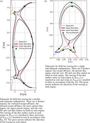
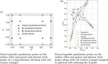
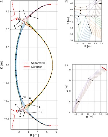
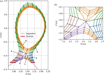
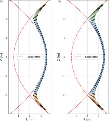
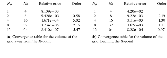
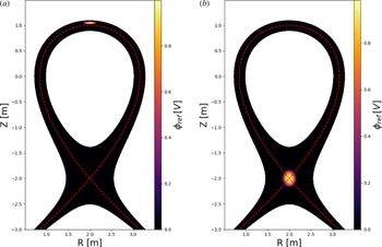

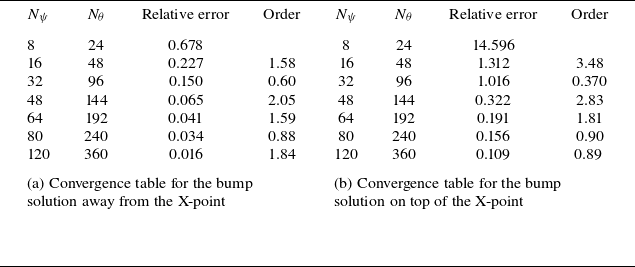
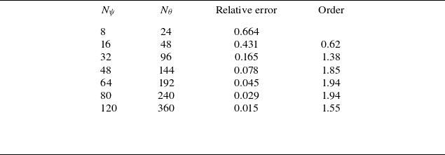

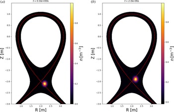
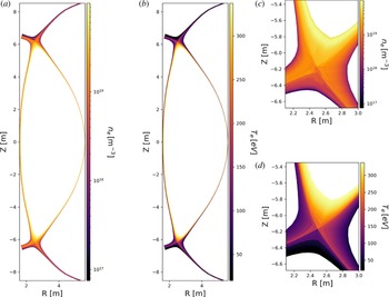
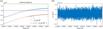

 Open access

