2. Computational setup

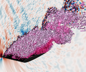
In this paper, we consider a NACA0012 aerofoil with a sharp TE at Reynolds number $50\ 000$. Two different free-stream Mach numbers ($0.3$ and $0.4$) and three incidence angles ($5^\circ$, $10^\circ$ and $15^\circ$) are explored. Under the current flow conditions, the aerofoil experiences a leading edge (LE) stall process as the angle of attack is increased, caused by laminar boundary layer separation. The pre-stall condition is an example of a classical laminar separation bubble. As the incidence angle is increased, the bubble is shifted towards the LE, eventually bursting due to an excessive adverse pressure gradient. In full-stall, the flow is characterised by instabilities such as Kelvin–Helmholtz vortex shedding in the separated shear layer (SSL), which develops into a von Kármán vortex street downstream of the TE. The instantaneous flow and sound fields are visualised for the stalled case in figure 1 by iso-surfaces of streamwise vorticity ($\omega _x$) coloured by streamwise velocity magnitude, and divergence of velocity contours ($\boldsymbol {\nabla }\boldsymbol {\cdot }\boldsymbol {u}$), respectively.

Figure 1.

Snapshot of streamwise vorticity iso-surfaces ($\omega _xL_c/a_\infty =\pm 8$) coloured by streamwise velocity (normalised). Dilatation $(\boldsymbol {\nabla }\boldsymbol {\cdot }\boldsymbol {u})L_c/a_\infty$ contours are shown in the $xy$-plane at $z=-0.5L_c$. (a) Isometric view; (b) side view.

2.1. Governing equations and numerical methods

A conservative form of the three-dimensional compressible Navier–Stokes equations written in a generalised coordinate system is used for the current direct numerical simulation (DNS):

(2.1)\begin{equation} \frac{\partial}{\partial t}\left(\frac{\boldsymbol{Q}}{J}\right)+ \frac{\partial}{\partial\xi_i}\left(\frac{\boldsymbol{E}_j-Re^{{-}1}_\infty M_\infty\boldsymbol{F}_j}{J}\,\frac{\partial\xi_i}{\partial x_j}\right)={-}\frac{a_\infty}{L_c}\,\frac{\boldsymbol{S}}{J}, \end{equation}

where the indices $i=1,2,3$ and $j=1,2,3$ denote the three dimensions, and $a_\infty$ is the ambient speed of sound. The vectors of the conservative variables, inviscid and viscous fluxes, are given by

(2.2)\begin{equation} \left.\begin{array}{c@{}} \boldsymbol{Q}=[\rho,\rho u,\rho v,\rho w,\rho e_{t}]^{\rm T},\\ \boldsymbol{E}_j=[\rho u_j,(\rho uu_j+\delta_{1j}p),(\rho vu_j+\delta_{2j}p),(\rho wu_j+\delta_{3j}p),(\rho e_{t}+p)u_j]^{\rm T},\\ \boldsymbol{F}_j=[0, \tau_{1j}, \tau_{2j}, \tau_{3j}, u_i\tau_{ji}+q_j]^{\rm T}, \end{array}\right\} \end{equation}

with the stress tensor and heat flux vector written as

(2.3a,b)\begin{equation} \tau_{ij}=\mu\left(\frac{\partial u_i}{\partial x_j}+\frac{\partial u_j}{\partial x_i}-\frac{2}{3}\,\delta_{ij}\,\frac{\partial u_i}{\partial x_i}\right), \quad q_j=\frac{\mu}{(\gamma-1)Pr}\,\frac{\partial T}{\partial x_j}, \end{equation}

where $\xi _i=\{\xi,\eta,\zeta \}$ are the generalised coordinates, $x_j=\{x,y,z\}$ are the Cartesian coordinates, $\delta _{ij}$ is the Kronecker delta, $u_j=\{u,v,w\}$, $e_{t}=p/[(\gamma -1)\rho ]+u_ju_j/2$, and $\gamma =1.4$ for air. The local dynamic viscosity $\mu$ is calculated by using Sutherland's law (White Reference White1991). In the current set-up, $\xi$, $\eta$ and $\zeta$ are aligned in the streamwise, vertical and lateral directions, respectively. The Jacobian determinant of the coordinate transformation (from Cartesian to generalised) is given by $J^{-1}=|\partial (x,y,z)/\partial (\xi,\eta,\zeta )|$ (Kim & Morris Reference Kim and Morris2002). The extra source term $\boldsymbol {S}$ on the right-hand side of (2.1) is non-zero within the sponge layer only, which is described in Kim, Lau & Sandham (Reference Kim, Lau and Sandham2010a,Reference Kim, Lau and Sandhamb). In this paper, the free-stream Mach and Reynolds numbers are defined as $M_\infty =u_\infty /a_\infty$ and $Re_\infty =\rho _\infty u_\infty L_c/\mu _\infty$. The governing equations are non-dimensionalised based on the aerofoil chord length $L_c$ for length scales, the ambient speed of sound $a_\infty$ for velocities, $L_c/a_\infty$ for time scales, and $\rho _\infty a^2_\infty$ for pressure. Temperature, density and dynamic viscosity are normalised by their respective ambient values: $T_\infty$, $\rho _\infty$ and $\mu _\infty$.

The governing equations given above are solved by using high-order accurate numerical methods developed specifically for aeroacoustic simulations on structured grids. The flux derivatives in space are calculated based on fourth-order pentadiagonal compact finite difference schemes with seven-point stencils (Kim Reference Kim2007). Explicit time advancing of the numerical solution is carried out by using the classical fourth-order Runge–Kutta scheme with Courant–Friedrichs–Lewy (CFL) number 1.0. Numerical stability is maintained by implementing sixth-order pentadiagonal compact filters for which the cutoff wavenumber (normalised by the grid spacing) is set to $0.8{\rm \pi}$ in interior regions and ramped up to ${\rm \pi}$ at the boundaries (Kim Reference Kim2010). In addition to the sponge layers used, characteristics-based non-reflecting boundary conditions (Kim & Lee Reference Kim and Lee2000) are applied at the far boundaries in order to prevent any outgoing waves from returning to the computational domain. Periodic conditions are used across the spanwise boundary planes as indicated earlier. On the aerofoil surface, no-slip wall boundary conditions are implemented (Kim & Lee Reference Kim and Lee2004).

A moving frame technique is used to initialise the simulations, which gradually ramps the velocity from zero to the free-stream value $(u_\infty, v_\infty, w_\infty )=(|\boldsymbol {u}|\cos (\alpha ), |\boldsymbol {u}|\sin (\alpha ), 0)$. Each simulation is run for a total of $T^*=t\,a_\infty /L_c=200$ non-dimensional time units. The approximate time step size (provided by the CFL number) is ${\rm \Delta} t\, a_\infty /L_c=1\times 10^{-4}$. Data are collected during the final 20 non-dimensional time units for post-processing of the acoustics signals. The spectra in this paper are presented based on either one-third or one-twelfth octave averaging. The sensitivity of the results to the time series length is tested in the Appendix.

2.2. Computational domain and grid

The computational domain is a rectangular cuboid with the aerofoil at the centre. The outer boundaries of the $xy$-plane (where $x$ and $y$ are the horizontal and vertical coordinates, respectively) are surrounded by a sponge layer through which numerical reflections are attenuated. The entire computational domain, the inner region (physical domain) where meaningful simulation data are obtained, and the sponge layer zone are defined as

(2.4)\begin{equation} \left. \begin{array}{c@{}} \mathcal{D}_\infty=\{\boldsymbol{x} \mid x/L_c\in[{-}9,9], y/L_c\in[{-}9,9], z/L_z\in[{-}1/2,1/2]\},\\ \mathcal{D}_{phys}=\{\boldsymbol{x} \mid x/L_c\in[{-}7,7], y/L_c\in[{-}7,7], z/L_z\in[{-}1/2,1/2]\},\\ \mathcal{D}_{sponge}=\mathcal{D}_\infty-\mathcal{D}_{phys}, \end{array}\right\} \end{equation}

where $L_z$ is the spanwise domain length. The aerofoil's leading and trailing edges are located at $x/L_c=-1/2$ and $1/2$, respectively. The default spanwise domain size is one chord length ($L_z=L_c$), unless stated otherwise. This is considered to be sufficient for reliable simulations in stall conditions. A numerical validation on this has been undertaken previously by the authors (Turner & Kim Reference Turner and Kim2020b).

The current numerical simulations are performed on a structured H-topology grid that is stretched in both the horizontal and vertical directions (uniform in span), with the smallest cells positioned on the aerofoil surface. Additional refinement is implemented in the wake region of the aerofoil, specifically the first two chord lengths above the aerofoil, which corresponds roughly to the wake height at the domain outlet, and the first two chord lengths downstream of the TE. A total of $(N_\xi, N_\eta, N_\zeta)=(1200,1120,326)$ grid cells are used in the three respective directions, distributed over 6720 processor cores on ARCHER. The full domain and grid with the aerofoil at the centre is shown in figure 2(a), with one in five points plotted. The grid lines are coloured by the streamwise component of velocity, which demonstrates the asymmetric distribution of points between the upper and lower half-planes. At the current Reynolds number, the aerofoil pressure side remains laminar and therefore requires less grid resolution than the suction side, where transition and separation occur. Additionally, in figure 2(b,c) a side view close-up near the aerofoil and the surface mesh are shown with one in four points plotted. The spanwise- and time-averaged surface mesh sizes in wall units are shown in figure 3. Approximate requirements for DNS mesh sizes have been suggested by Georgiadis, Rizzetta & Fureby (Reference Georgiadis, Rizzetta and Fureby2010) as $10\leq {\rm \Delta} x^+\leq 20$, ${\rm \Delta} y^+<1$ and $5\leq {\rm \Delta} z^+\leq 10$. The current mesh sizes remain either within or below these requirements over the full aerofoil surface. An extensive validation of the current numerical set-up has been carried out in Turner & Kim (Reference Turner and Kim2020b), including verification of the spanwise domain size and comparison to experiments for aerodynamic coefficients. In addition, the wall mesh sizes away from the wall have been compared in the previous paper to the local Kolmogorov micro-scale $\eta =(\nu ^3/\epsilon )^{1/4}$. It was found that the turbulent regions mostly satisfy $J^{1/3}<4\eta$, with a maximum value around $5.5\eta$. Additionally, a grid refinement study for the far-field noise prediction is included in the Appendix.

Figure 2.

Computational mesh used in the numerical set-up. (a) Side view of full domain with grid lines coloured by streamwise velocity $u/a_\infty$ (every fifth point shown in each direction). (b) Close-up of NACA0012 profile (every fourth point shown in each direction). (c) Aerofoil surface mesh (every fourth point shown in each direction).

Figure 3.

Time- and spanwise-averaged grid sizes in wall units over the aerofoil surface. ${\rm \Delta} s$ and ${\rm \Delta} n$ represent the body-fitted and wall-normal spacings, respectively.

The computation is parallelised via domain decomposition and message passing interface (MPI) approaches. The compact finite difference schemes and filters used are implicit in space due to the inversion of pentadiagonal matrices involved, which requires a precise and efficient technique for the parallelisation in order to avoid numerical artefacts that may appear at the subdomain boundaries. A parallelisation approach based on quasi-disjoint matrix systems (Kim Reference Kim2013) offering super-linear scalability is used in the present paper.

2.3. Definition of variables for statistical analysis

Data processing and analysis are carried out upon the completion of each simulation. The far-field (acoustic) pressure is defined as

(2.5)\begin{equation} p_a(\boldsymbol{x},t)=p(\boldsymbol{x},t)-\bar{p}(\boldsymbol{x}), \end{equation}

where $\bar {p}(\boldsymbol {x})$ is the time-averaged pressure. Following the definitions used in Goldstein (Reference Goldstein1976), the Fourier transform of $p_a$ can then be calculated as

(2.6)\begin{equation} P_a(\boldsymbol{x},f,T)=\int_{{-}T}^{T}{p_a(\boldsymbol{x},t)\, {\rm e}^{2{\rm \pi} ift}\,{\rm d} t}, \end{equation}

and the one-sided frequency-based power spectral density (PSD) function as

(2.7)\begin{equation} S_{ppa}(\boldsymbol{x},f)=\lim_{T\rightarrow\infty}\frac{P_a(\boldsymbol{x},f,T)\,P_a^*(\boldsymbol{x},f,T)}{T}, \end{equation}

where ‘$*$’ denotes a complex conjugate. The same definitions can also be used to calculate the spectra of other variables. The sound power spectra are calculated by integrating the fluctuating pressure PSD between two observer angles $\theta _1$ and $\theta _2$:

(2.8)\begin{equation} W(\theta_1,\theta_2,f)=\frac{Rb}{\rho_\infty a_\infty}\int^{\theta_2}_{\theta_1}S_{ppa}(\theta,f) \, {\rm d} \theta, \end{equation}

where $R=10L_c$ is the distance from the aerofoil mid-chord to the observers, and $b$ is the span of the integration surface, taken as $25L_c$ for consistency with the FWH calculations. For the majority of the spectra presented in this paper, $\theta _2-\theta _1=20^\circ$, and $\theta _0$ is the middle observer angle. We also define two normalised frequencies used throughout the paper:

(2.9)\begin{equation} \left.\begin{array}{c@{}} St_u=fL_c/u_\infty, \\ St_a=fL_c/a_\infty. \end{array}\right\} \end{equation}

3. Far-field extrapolation approach

In this paper, the far-field noise is calculated by using the FWH method (Ffowcs Williams & Hawkings Reference Ffowcs Williams and Hawkings1969) based on two different approaches: (1) solid wall, and (2) permeable surface integrations. Theoretically, a permeable integration surface is capable of capturing both surface dipoles and volume quadrupoles (if it surrounds all the turbulence). This kind of approach is often preferable over calculating directly volume quadrupole terms due to the excessive cost (in terms of both time and memory) required. One of the first permeable-surface-based FWH formulations is the time domain solution proposed by Di Francescantonio (Reference Di Francescantonio1997), which is used in the current study:

(3.1)\begin{align} 4{\rm \pi}\,p_P(\boldsymbol{x},t)&=\int\left[\frac{\rho_\infty\dot{U}_in_i}{r|1-M_r|^2} +\frac{\rho_\infty U_in_ia_\infty(M_r-M^2)}{r|1-M_r|^3} \right]_{ret} {\rm d} S_P \nonumber\\ &\quad +\int\left[\frac{\dot{F}_i\hat{r}_i}{a_\infty r|1-M_r|^2} +\frac{\dot{F}_i\hat{r}_i-F_iM_i}{r^2|1-M_r|^2} +\frac{F_i\hat{r}_i(M_r-M^2)}{r^2|1-M_r|^3}\right]_{ret} {\rm d} S_P \end{align}

and

(3.2a–c)\begin{equation} F_i={\mathsf{L}}_{ij}n_j, \quad U_i=u_i+[(\rho/\rho_\infty-1)](u_i-v_i), \quad {\mathsf{L}}_{ij}=p^\prime\delta_{ij}+\rho u_i(u_j-v_j), \end{equation}

where $v_i$ is the surface velocity, $n_j$ is the surface normal, and $\delta _{ij}$ is the Kronecker delta. Dotted variables indicate the time derivative, while subscript $ret$ indicates that variables are analysed at the retarded time $\tau =t-r/a_\infty$. The above integration is performed on the permeable surface $S_P$ that encloses the aerofoil and full wake. For problems involving rectilinear motion, the retarded time can be determined uniquely via the Garrick triangle (Garrick & Watkins Reference Garrick and Watkins1953), extended below for two-dimensional mean flow velocity:

(3.3)\begin{equation} r=\frac{M_1d_1+M_2d_2+\sqrt{(M_1d_1+M_2d_2)^2+(1-M_1^2 -M_2^2)[d_1^2+d_2^2+d_3^2]}}{1-M_1^2-M_2^2}, \end{equation}

where $M_i=v_i/a_\infty$ and $d_i=(x_o-x_s,y_o-y_s,z_o-z_s)$, with subscripts $o$ and $s$ representing observer and source, respectively. Additionally, $M_r=\boldsymbol {M}\boldsymbol {\cdot }\hat {\boldsymbol {r}}$, where $\boldsymbol {r}$ is the radiation vector, and $\hat {\ }$ indicates a unit length.

Meanwhile, a second FWH calculation is performed by using a solid-surface integration on the aerofoil. Equation (3.1) is simplified considerably by noting that $u_i=v_i$ due to the no-slip condition. This returns the well-known formulation 1A proposed by Farassat & Succi (Reference Farassat and Succi1980):

(3.4)\begin{align} 4{\rm \pi}\,p_S(\boldsymbol{x},t)&=\int \left[\frac{\dot{p}^\prime n_i\hat{r}_i}{a_\infty r|1-M_r|^2}+\frac{p^\prime n_i\hat{r}_i-p^\prime M_in_i}{r^2|1-M_r|^2}\right]_{ret} {\rm d} S_S \nonumber\\ &\quad +\int \left[\frac{(M_r-M^2)p^\prime n_i\hat{r}_i}{r^2|1 -M_r|^3}+\frac{\rho_\infty a_\infty v_in_i (M_r-M^2)}{r^2|1 -M_r|^3}\right]_{ret} {\rm d} S_S. \end{align}

From here on, we refer to (3.4) and (3.1) as the FWH-S and FWH-P solutions, respectively. As mentioned earlier, the FWH-P solution is expected to contain all noise components in full. However, the FWH-S solution consists mainly of the dipole noise and partially of the secondary quadrupole noise scattered by the aerofoil body. If we focus on the primary dipole component of the FWH-S solution, then the following approximations could be used:

(3.5)\begin{equation} \left.\begin{array}{c@{}} p_{{Total}}=p_P,\\ p_D\simeq p_S,\\ p_Q\simeq p_P - p_S. \end{array}\right\} \end{equation}

It is important to also account for the spanwise periodic boundary condition present in the numerical simulations within the FWH integration. This is essential to obtain the same radiated sound amplitude as signal probes positioned in the grid. This can be accomplished by performing repeated surface integrations on spanwise-shifted domains until a converged result is obtained. Despite the aerofoil being effectively infinite in span, convergence occurs due to $r$ increasing and $n_i\hat {r}_i\rightarrow 0$ as the $z$ coordinate increases relative to the observer. For the current problem, 25 spanwise domain lengths (25 chords) were required to reach convergence.

The computational cost saving offered by the permeable approach (compared to volume integration) is especially useful for the current DNS cases, which produce large datasets of size ${\sim }10$ TB. Despite this clear advantage, there are some practical considerations required to ensure reliable results. Strictly speaking, the surface must surround the entire turbulent region for the quadrupole sound to correctly determined. Additionally, the surface should be placed in a region of adequate grid resolution to capture the desired acoustic wavelengths. Often these restrictions are not practical. It is a fairly common practice to truncate the surface in the downstream direction – usually, to reduce the computation cost or due to excessive downstream grid stretching. For problems with large wakes or jets, surface truncation can result in the hydrodynamic perturbations perpendicularly crossing the surface end-plane. In doing this, the fluid perturbations manifest as an unphysical noise source in the FWH equations. Several treatments have been proposed to minimise end-plane errors. One of the simplest is to use an ‘open surface’, where the end-cap is ignored during integration. This has the obvious drawback of missing some of the acoustic information, mainly for observers directly downstream. Another common technique is to employ additional averaged end-caps (Shur, Spalart & Strelets Reference Shur, Spalart and Strelets2005). This method aims to force phase interference in the time signals of the convected disturbances due to the different retarded times on each end-plane. Although this approach can be effective, it is not exact, and there is a danger of choosing the end-plane locations arbitrarily if the results are not compared against experimental data. Additionally, the effectiveness of the averaging approach relies on a contrast between the convection speeds of the turbulence and the sound. At $M_\infty =0.4$ this could pose a problem for sound waves convecting against the mean flow. Experimental acoustic data for stalled aerofoils is scarce, especially under the current flow conditions. Consequently, we prefer to minimise additional treatments where possible, opting to contain as much of the wake as possible within the surface (rather than truncating).

Four surfaces shown in figure 4 are tested to verify the consistency of the results. The first surface (S1) is a tight-fit truncated surface, avoiding the coarse grids in the downstream sponge region. Comparatively, S2 extends the full length of the computational domain. Both open and closed variants of S2 are considered. S3 and S4 are full-length surfaces with increasing vertical offset from the wake. Figure 5 shows the far-field data predicted with the four integration surfaces. The normalised sound power is shown for $\theta _0=90^\circ$ in figure 5(a), while directivity plots are shown for $St_u=0.75$, $3.0$ and $12.0$ in figures 5(b–d). All four surfaces obtain comparable results for spectra and directivity at mid-to-high frequencies $St_u>3.0$. At lower frequency, the S2 closed surface shows significant differences from the others despite the end-plane position at the domain exit. Most notably, it incorrectly predicts the von Kármán shedding frequency $St_u=0.75$, which is known from previous work (Turner & Kim Reference Turner and Kim2020a). A consistent result is obtained by the surfaces S3 and S4 at all frequencies, which demonstrates convergence of the top and bottom surface boundary locations. The open S1 and S2 results are also comparable to S3 and S4, except for directly upstream at $St_u=0.75$ and downstream at $St_u=3.0$. The downstream lobes predicted by S1 and S2 at $St_u=3.0$ are suspect since the surface end-plane is open. Additionally, the lobes are gradually reduced by loosening the vertical surface boundaries.

Figure 4.

FWH integration surfaces (S1–S4) shown alongside the unsteady flow field. The aerofoil wake is visualised by iso-surfaces of normalised Q-criterion ($QL^2_c/a^2_\infty$) coloured by vertical velocity.

Figure 5.

Far-field noise predictions obtained with the four FWH integration surfaces (see figure 4). (a) One-twelfth octave averaged normalised sound power for $\theta _0=90^\circ$. One-third octave averaged sound directivity plots based on the magnitude of acoustic pressure Fourier transform at $R=10L_c$ for (b) $St_u=0.75$, (c) $St_u=3.00$, and (d) $St_u=12.00$.

The four surfaces are also tested by comparing with a direct noise computation obtained by a probe positioned at $\boldsymbol {x}_o=(0,3L_c,0)$. The resulting spectra are shown in figure 6. The best agreement is obtained by using either surface S3 or surface S4. The only exception is for very high frequencies ($St_u>20$), where the probe solution begins to suffer from dissipation due to grid stretching. The result demonstrates that ignoring the end-cap data does not significantly impact the accuracy of the FWH prediction if the surface is carefully selected (and extends the full length of the wake). Consequently, the S4 surface is used for the calculations carried out in this paper.

Figure 6.

PSD of acoustic pressure (one-twelfth octave averaged) obtained by a probe at $\boldsymbol {x}_o=(0,3L_c,0)$. Comparison is made with the FWH-P predictions based on the surfaces (a) S1, S2, and S2 closed, and (b) S3 and S4.

4. Significance of quadrupole noise contributions

In previous work by the authors, the dipole noise was investigated under the same flow conditions (Turner & Kim Reference Turner and Kim2020a). Although it was not the focus of the previous study, there was convincing evidence of significant quadrupole sources, particularly for near- and full-stall conditions. The divergence of velocity contours shown in figure 1 indicates how noise radiates from the SSL close to the LE. Furthermore, sound waves are radiated from the vortex roll-ups in the wake seen in figure 1(b). This is in contrast to a typical dipole sound field expected for low angles of incidence, radiated primarily from the TE.

The far-field sounds predicted by the FWH-S and FWH-P approaches are compared in this section to determine approximately the increase in total noise due to quadrupole sources. The PSD functions of acoustic pressure predicted by the two approaches are shown in figure 7(a,b) for observer angles $\theta =90^\circ$ and $270^\circ$. At $\theta =90^\circ$, increased noise amplitude is predicted by the FWH-P approach for most of the frequency range. Most notably, in the range $4\leq St_u\leq 30$, the increase is approximately 10 dB or more, indicating that the quadrupole contribution is dominant. This differs from the aerofoil underside, $\theta =270^\circ$, where the two solutions are more comparable except for at low frequencies. The difference between the radiated noise above and below the aerofoil is due to two reasons. First, there should be some sound blockage due to the turbulent flow appearing on only the aerofoil suction side, resulting in higher quadrupole levels above the aerofoil. This should affect sound waves generated by the SSL more severely than those from large structures in the wake, possibly explaining why an increase is observed for low frequencies at $\theta =270^\circ$. Second, the dipole noise is biased towards the lower half-plane due to the positive incidence angle. This can be explained by considering the Doppler factor term $|1-M_r|^2$ appearing in the leading term of (3.4), which differs by approximately a factor of 1.5 between the upper and lower half-planes.

Figure 7.

PSD functions of acoustic pressure (one-twelfth octave averaged) compared for FWH-S ($p_D$) and FWH-P ($p_{{Total}}$) predictions for $\alpha =15^\circ$. (a) $\theta =90^\circ$; (b) $\theta =270^\circ$.

Third octave band directivity plots are shown in figures 8(a–f) based on the magnitude of acoustic pressure Fourier transform at six Strouhal numbers: $St_u=0.75$, $1.5$, $3.0$, $6.0$, $12.0$ and $24.0$. In addition to the FWH-S ($p_D$) and FWH-P ($p_{{Total}}$) solutions, the Fourier transform of $p_Q$ is also included. At the low-frequency peak ($St_u=0.75$), the maximum levels for dipole and quadrupole noise are comparable, although the main radiation directions differ. The quadrupole sound is directed upstream primarily, where the dipole sound is weakest. Consequently, the total noise radiation is less restricted towards the vertical directions than it is for the dipole-only component. At $St_u=1.5$, the quadrupole sound increases relative to the dipole sound, becoming comparable or larger in every direction except directly below the aerofoil. Again, the largest quadrupole noise amplitude is radiated upstream, near $\theta =150^\circ$. For Strouhal numbers $St_u=3.0$, $6.0$ and $12.0$, the quadrupole sound remains dominant. However, the largest sound amplitude is directed vertically, for $90^\circ \leq \theta \leq 120^\circ$. For $St_u=24.0$, strong asymmetry is predicted by the FWH-P approach between the upper and lower half-planes. As mentioned previously, this could be due to blockage of the quadrupole sound on the suction side due to the body. This would be most significant for angles slightly upstream since the wake noise will also be blocked partially. Another possibility is a strong negative correlation between the dipole and quadrupole noise in this direction. A similar observation was also made by Spalart et al. (Reference Spalart, Belyaev, Shur, Strelets and Travin2019) for a noise source on one side of a fuselage.

Figure 8.

One-third octave averaged sound directivity plots for $M_\infty =0.4$ based on the magnitude of acoustic pressure Fourier transform (see (2.6)) at $R=10L_c$ for (a) $St_u=0.75$, (b) $St_u=1.5$, (c) $St_u=3.0$, (d) $St_u=6.0$, (e) $St_u=12.0$, and (f) $St_u=24.0$.

The dominance of quadrupole sound in the upper half-plane is initially surprising considering the scaling laws of Curle ($p^2_Q=O(M^8)$ and $p^2_D=O(M^6)$, indicating $p^2_Q/p^2_D\sim M^2$). However, an important consideration is that for separated flows, the relevant local Mach numbers for quadrupoles and dipoles might not be the same. For instance, the local convection speed near the TE (relevant for dipoles) is typically lower than the SSL convection speed (relevant for quadrupoles). On the contrary, for attached flow cases, the boundary layer convection speed is probably determinant for both sources of noise. A good estimate for $p_Q/p_D$ may be attainable if the correct velocities can be calculated. However, this is not a straightforward task since there are likely multiple quadrupole sources occurring in different regions of the flow. To better demonstrate this, snapshots of the acoustic pressure field are shown at specific frequencies in figure 9. The bandpass filtered field is achieved with the equation

(4.1)\begin{equation} \left.\begin{array}{c@{}} \widetilde{p_a}(\boldsymbol{x},t)=\mathcal{F}^{{-}1}\{W(f)\,\mathcal{F}[p_a(\boldsymbol{x},t)]\},\\ W(f)=\exp[-\beta(f-f_p)^2/{\rm \Delta} f^2]+\exp[-\beta(f+f_p)^2/{\rm \Delta} f^2], \end{array}\right\} \end{equation}

where $\mathcal {F}$ and $\mathcal {F}^{-1}$ represent the Fourier and inverse Fourier transforms, respectively, and $W(f)$ is a narrow-band frequency filter with a bandwidth ${\rm \Delta} f^*=1$ at target frequency $f_p$. The coefficient $\beta =20$ determines the steepness of the window function. The filtered pressure snapshots are shown at the end of the simulation. At low frequencies, $St_u=0.75$ and $3.5$, it is clear how sound waves are emitted directly from the near wake. This is a clear indication of low-frequency quadrupole sound (since the waves are not emitted from the aerofoil surface), hence the increase at low frequencies observed previously. At the von Kármán shedding frequency, the low-frequency wake noise is directed primarily upstream, which explains the strong upstream directivity for the quadrupole noise in figure 8(a). As the frequency is increased (see $St_u=6.00$ and $10.00$), interference patterns emerge, especially on the aerofoil suction side, indicating multiple noise sources. At high frequencies (see $St_u=20.00$ and $40.00$) it is clear how the separated shear layer directly above the aerofoil begins to play a more major role in the production of the noise.

Figure 9.

Filtered fluctuating pressure field $\widetilde {p_a}$ obtained at the mid-span location for (a) $St_u=0.75$, (b) $St_u=3.50$, (c) $St_u=6.00$, (d) $St_u=10.00$, (e) $St_u=20.00$, and (f) $St_u=40.00$.

The dominant flow features at the various frequencies are also identified by replotting with more appropriate contour levels. Figure 10 shows three-dimensional iso-surfaces of the filtered fluctuating pressure on the aerofoil suction side at four frequencies, $St_u=0.75$, $3.5$, $6.0$ and $20.0$. The sound waves are shown in the $z/L_c=-L_z/2$ and $y/L_c=0$ planes. At $St_u=0.75$, the dominating flow structure is the von Kármán vortex street. The highest intensity occurs in the near wake as indicated by the sound waves in figure 9(a). The structures are relatively uniform in the spanwise direction, which results in cylindrical sound propagation and minimal interference patterns. The filtered pressure field at $St_u=3.50$ shows a combination of turbulent structures in the near wake, as well as spanwise-coherent vortices around one chord length downstream. The spanwise vortices likely play a meaningful role in the generation of the noise as indicated by the sound waves emitted from the wake in figure 9(b). At $St_u=6.0$, vortices in the separated shear layer are highlighted in addition to small-scale structures near the TE and spanwise vortices in the wake. The multiple source regions lead to a more complex sound field with various interference effects. Similarly, at $St_u=20.0$, Kelvin–Helmholtz vortices and the subsequent breakdown to turbulence also dominate the flow field along with small-scale structures near the TE. At high frequencies, it is also interesting to note that the sound field becomes more three-dimensional (as seen in the $y=0$ plane) due to the breakdown of the dominating flow structures in the spanwise direction.

Figure 10.

Iso-surfaces of the filtered fluctuating pressure $\widetilde {p_a}$ shown on the aerofoil suction side: (a) $St_u=0.75$, (b) $St_u=3.50$, (c) $St_u=6.00$, and (d) $St_u=20.00$.

In figure 11(a–d) the spectral content at specific angles $\theta _0=120^\circ$, $150^\circ$, $210^\circ$ and $250^\circ$ is investigated more closely. The figure shows normalised sound power, calculated over $20^\circ$ observer bands as in (2.8). Solutions based on $p_{{Total}}$ (FWH-P), $p_D$ (FWH-S) and $p_Q$ are included. The figure provides further confirmation that the quadrupole sound is the larger of the two sources in the upper half-plane. At $\theta _0=120^\circ$, the quadrupole noise is more than 10 dB greater than the dipole in the range $3< St_u\leq 40$. Moving the observer further upstream tends to reduce the lower frequency bound where quadrupole noise begins to dominate. For $\theta _0=150^\circ$, the quadrupole exceeds the dipole noise for the full frequency range by as much as 10 dB at low frequencies and 20 dB at high frequencies. The larger difference is due partly to significantly lower levels of dipole sound in the upstream/downstream directions. The low-frequency increase to the total noise due to quadrupoles differs from previously published results at low angles of attack where quadrupole contributions were limited to high frequencies (Wolf et al. Reference Wolf, Azevedo and Lele2012). As previously suggested, this is likely caused by radiation directly from the large-scale vortex shedding in the wake. For the equivalent upstream angle in the lower half-plane ($\theta _0=210^\circ$), the quadrupole noise dominates a similar frequency range. However, the amplitude increase (relative to the dipole sound) is usually milder, between 0 and 5 dB. Comparatively, for $\theta _0=250^\circ$, comparable amplitude levels are observed for both dipole and quadrupole results over most frequencies. When the amplitudes are similar, meaningful phase interactions are possible between the two sources. In this instance, constructive interference occurs for the low-frequency peaks when $St_u<2$, while at high frequencies the two sources appear to interfere destructively, reducing the overall radiated noise.

Figure 11.

Comparison of one-twelfth octave averaged normalised sound power predictions obtained based on $p_D$ (FWH-S), $p_{{Total}}$ (FWH-P) and $p_Q$ ($p_{{Total}}-p_D$) for $\alpha =15^\circ$ at four observer angles: (a) $\theta _0=120^\circ$, (b) $\theta _0=150^\circ$, (c) $\theta _0=210^\circ$, and (d) $\theta _0=250^\circ$. Sound power is calculated over a $20^\circ$ observer range.

5. Influence of Mach number on quadrupole noise

In this section, an additional simulation is carried out at the free-stream Mach number $M_\infty =0.3$ to determine the effect of mean flow speed on the quadrupole noise. The aerofoil profile and angle of attack remain fixed. Figure 12 shows the sound fields obtained at the two flow speeds based on the divergence of velocity contours ($\boldsymbol {\nabla }\boldsymbol {\cdot }\boldsymbol {u}$). There is a visibly large difference between the two cases, with the $M_\infty =0.3$ case demonstrating something closer to the more classical dipole sound radiation expected from a sharp TE aerofoil (although sound waves are also emitted from the SSL). At the higher Mach number, the quadrupole sources become qualitatively more significant. It is interesting to note how sound waves are generated from the wake for $M_\infty =0.4$, which do not appear (visibly) for $M_\infty =0.3$.

Figure 12.

Normalised divergence of velocity contours $(\boldsymbol {\nabla }\boldsymbol {\cdot }\boldsymbol {u})L_c/a_\infty$ shown in the $xy$-plane at $z/L_c=0$ for (a) $M_\infty =0.4$ and (b) $M_\infty =0.3$. The wake is visualised by the normalised Q-criterion ($QL^2_c/a^2_\infty =1.0$).

The radiated sound power (see (2.8)) produced by both solid and permeable FWH approaches is compared for the two Mach numbers in figures 13(a,b) for $\theta _0=90^\circ$ and $\theta _0=120^\circ$, respectively, versus $St_a$. The contribution from direct quadrupole sound remains significant for the lower Mach number case, although the increase in total noise begins at a slightly higher frequency compared to $M_\infty =0.4$. This observation is consistent with the divergence field in figure 12, which clearly showed waves emitted from the large-scale structures in the wake in the higher Mach number case. The change in sound power level (PWL) spectra (increase in total noise due to the direct quadrupole contribution) can be calculated as

(5.1)\begin{equation} {\rm \Delta} {PWL}_{T}=10\log_{10}(W_{{Total}}/W_{D}), \end{equation}

where ${\rm \Delta} {PWL}_{T}$ is plotted in figure 14 against the Strouhal number $St_u$. At $\theta _0=90^\circ$, there is a fairly constant increase in total noise for $St_u\gtrsim 5.0$, with mean values 6.35 and 8.70 dB for $M_\infty =0.3$ and $0.4$, respectively. At $\theta _0=120^\circ$, where the quadrupole sound tends to radiate more strongly (see figure 8), the noise increase rises significantly for the higher Mach number case.

Figure 13.

One-twelfth octave averaged normalised sound power versus $St_a$ obtained with the FWH-S ($p_D$) and FWH-P ($p_{{Total}}$) approaches at two Mach numbers, $M_\infty =0.4$ and $0.3$. (a) $\theta _0=90^\circ$; (b) $\theta _0=120^\circ$.

Figure 14.

Increase in total noise due to quadrupole sources ${\rm \Delta} {PWL}_{T}$ (calculated using one-third octave averaging). (a) $\theta _0=90^\circ$; (b) $\theta _0=120^\circ$.

Third octave directivity plots for $M_\infty =0.3$ are shown in figures 15(a–f) for comparison with the higher Mach number case in figure 8. In figure 15, $p_{{Total}}$ (FWH-S), $p_D$ (FWH-P) and isolated $p_Q$ sound predictions are shown at the Strouhal numbers $St_u=0.75$, $1.5$, $3.0$, $6.0$, $12.0$ and $24.0$. For the three highest frequencies, a similar trend is observed as for the $M_\infty =0.4$ case. The largest radiated noise amplitude is in the upper half-plane close to $\theta =120^\circ$, with the quadrupole noise dominating there, and at other observer angles except around $240^\circ$. At the lower three frequencies ($St_u=0.75$, $1.5$, $3.0$), there is no clearly dominant radiation angle for the quadrupole sound. This differs from the results for $M_\infty =0.4$, which showed strong radiation in the upstream direction for low frequencies. This difference could be due to the noise radiated from the downstream wake in the higher Mach number case. Figure 12 shows that a component of the wake noise radiates in the upstream direction. (This is most clear on the aerofoil underside where there is less interference from other sources.)

Figure 15.

One-third octave averaged sound directivity plots for $M_\infty =0.3$ based on the magnitude of acoustic pressure Fourier transform (see (2.6)) at $R=10L_c$ for (a) $St_u=0.75$, (b) $St_u=1.5$, (c) $St_u=3.0$, (d) $St_u=6.0$, (e) $St_u=12.0$, and (f) $St_u=24.0$.

To approximate the Mach number scaling for dipoles and quadrupoles in the current simulations, we can consider the relative changes to $p_D$ and $p_Q$. The Mach number scaling exponent can be determined by assuming a power-law relationship

(5.2)\begin{equation} \frac{W(St_a)|_{M_A}}{W(St_a)|_{M_B}}=\left(\frac{M_A}{M_B}\right)^{N_a}, \end{equation}

where $W$ is the sound power spectra (2.8) based on $St_a$, calculated from either the dipole $p_D$ or the quadrupole $p_Q$ time signals. This rearranges to the following expression for $N_a$:

(5.3)\begin{equation} N_a=\frac{\log[W(St_a)|_{M_A}/W(St_a)|_{M_B}]}{\log(M_A/M_B)}. \end{equation}

An alternative expression for the scaling exponent can be obtained based on the power spectra as a function of $St_u$ (rather than $St_a$), which provides

(5.4)\begin{equation} \frac{W(St_u)|_{M_A}\times M_A}{W(St_u)|_{M_B}\times M_B}=\left(\frac{M_A}{M_B}\right)^{N_u} \end{equation}

and

(5.5)\begin{equation} N_u=\frac{\log[W(St_u)|_{M_A}/W(St_u)|_{M_B}]}{\log(M_A/M_B)}+1. \end{equation}

The factor $M_A/M_B$ is included on the left-hand side of (5.4) due to the definition of the PSD as the power per unit frequency (in this case per unit $St_u$). The calculated values for $N_u$ and $N_a$ are shown in figure 16(a–h) at four observer angles, $\theta _0=60^\circ$, $90^\circ$, $120^\circ$ and $150^\circ$. The outcome is non-trivial, with a strong dependence on frequency, frequency normalisation and observer angle. Consistent scaling against $St_a$ may suggest that sound scattering plays a vital role in determining the radiated sound. Alternatively, more convincing results in plots versus $St_u$ imply that coherent hydrodynamic features are important. It appears that the Mach number scaling based on $St_u$ produces the most consistent trend (values of $N_u$) for the $\theta _0=60^\circ$ and $90^\circ$ observers regarding both dipole and quadrupole sources. At $\theta _0=60^\circ$, the quadrupole noise oscillates around mean value $N_u=6.5$ in the range $5\leq St_u\leq 25$. This is close to the theoretical value $N_u=7$ suggested by Spalart (Reference Spalart2013) for quadrupoles in the presence of dipoles. At $\theta _0=90^\circ$, the average value is $N_u=8.1$ in the same range, close to the classical value $N=8$. However, the dipole noise is close to the theoretical value of $N_u=6$ only in a short range $15\leq St_u\leq 22$. For $\theta _0=120^\circ$ and $150^\circ$, neither $N_a$ nor $N_u$ provides a consistent trend for the quadrupole noise scaling. On the other hand, for dipole sound, the $N_a$ result is more convincing than that for $N_u$. The mean values of $N_a$ in the range $2\leq St_a\leq 10$ are $N_a=4.0$ and $4.9$, respectively, for $\theta _0=120^\circ$ and $150^\circ$. $N_a=4.9$ is close to the value observed typically for turbulent boundary layer scattering at a sharp TE, $N_a=5$. One possible explanation for the rapidly increasing $N$ values at high frequency is that the sound scaling based on the free-stream Mach number becomes less appropriate. The filtered flow field in figure 10 suggests that multiple flow regions are responsible for the noise at high frequencies. This includes Kelvin–Helmholtz vortices in the shear layer, turbulent flow near the TE, and spanwise wake vortices. Since all of these regions have different local flow speeds, it is difficult to determine the best value to use for the calculation of the sound scaling.

Figure 16.

Mach number scaling exponents $N_u$ and $N_a$ due to increasing the Mach number from $M_\infty =0.3$ to $0.4$. The values of $N_u$ (see (5.5)) and $N_a$ (see (5.3)) are calculated as the difference in sound power spectra based on $St_u$ and $St_a$, respectively (calculated using one-third octave averaging). (a,b) $\theta _0=60^\circ$; (c,d) $\theta _0=90^\circ$; (e,f) $\theta _0=120^\circ$; (g,h) $\theta _0=150^\circ$.

There are some similarities in the scaling exponent trends obtained for dipole and quadrupole sound, especially at $\theta _0=60^\circ$ and $90^\circ$. It is expected that the two sources are correlated, and therefore share some resemblance. However, the degree of similarity might indicate a more direct relationship between the dipole and quadrupole predictions. A possible explanation is identified by considering that the FWH-S approach contains a quadrupole sound component due to scattering by the aerofoil body. The current results suggest that the scattered quadrupole sound could be comparable or dominant to the dipole source radiation from the surface. Additionally, for $\theta _0=120^\circ$ and $150^\circ$, it is worth noting that the dipole noise scales closer to the theoretical value when the scaling exponent is calculated based on $St_a$. This could also be an indication of significant sound scattering phenomena. This is supported by figure 10, which shows the dominant flow structures for mid-to-high frequencies away from the wall (or aft of the TE), indicating that TE scattering may not be significant. Another indication of this was provided in the previous paper by the authors (Turner & Kim Reference Turner and Kim2020a). It was shown that for the mid-to-high frequencies, the wall pressure fluctuations were both weaker and had reduced chordwise phase variation compared to lower angles of attack, possibly indicating acoustics pressure disturbances.

6. Influence of incidence angle on quadrupole noise

In this section, the full-stall case is compared to pre-stall ($\alpha =5^\circ$) and near-stall ($\alpha =10^\circ$) conditions. The two additional datasets are carried out based on $M_\infty =0.4$ with $L_z=0.2L_c$ for the pre-stall case, and $L_z=L_c$ for the near-stall case (Turner & Kim Reference Turner and Kim2020a). Figure 17 compares the divergence of velocity and local Mach number fields for the three incidence angles. At the lowest incidence angle, there is a laminar separation bubble around the mid-chord location. Upon reattachment, the flow transitions to turbulence, remaining attached until the TE point. Increasing the angle of attack causes the separation bubble to shift towards the LE. At $\alpha =10^\circ$, the aerofoil is near the maximum lift condition. There is a short bubble near the LE and a turbulent boundary layer over the majority of the suction surface. Some separation is also observed near the TE intermittently. Above this angle, the bubble bursts, leading to the full stall condition seen previously in this paper.

Figure 17.

(a–c) Instantaneous divergence of velocity fields produced at the mid-span location for the three angles of attack $\alpha =5^\circ$, $\alpha =10^\circ$ and $\alpha =15^\circ$. (d–f) Local Mach number fields. Specific contour bands $M=0.5$, $0.525$ and $0.55$ shown in greyscale.

The sound field produced by the pre-stall case radiates primarily from the TE, except for some sound waves from the transition/reattachment region (possibly due to quadrupole sources appearing there). On the other hand, the near- and full-stall cases seem to radiate noise mainly from the SSL and downstream wakes. It is evident from the divergence fields that the noise produced at higher angles of attack also contains increased amplitude high-frequency waves. This is an expected outcome since the transition occurs further upstream at higher incidence angles. Another factor is the increased flow velocity near the transition point. For example, the $\alpha =10^\circ$ case experiences transition and reattachment of the laminar separation bubble within the first quarter chord, whereas the transition occurs around the mid-chord in the pre-stall condition where the local Mach number is lower. The instantaneous snapshots of the local Mach number field in figure 17 show higher and more consistent values along the edge of the SSL for the near-stall case compared to full-stall. Conversely, the full-stall case has higher Mach number values directly downstream of the TE, possibly indicating stronger quadrupole noise from the eddies generated there.

Figure 18 shows the radiated power spectra predicted by FWH-S ($p_D$) and FWH-P ($p_{{Total}}$) at the three angles of attack. The dipole results predicted by FWH-S have been discussed in detail in the previous paper by the authors (Turner & Kim Reference Turner and Kim2020a). Here they are repeated in order to analyse the trend changes when quadrupole sources are also included. The dipole noise can be separated into three frequency bands where different behaviours are observed. At low frequencies, increased broadband noise is observed for the near- and full-stall cases, with additional broad peaks due to wake shedding. At medium frequencies, the results are more similar for all angles of attack. Finally, at high frequencies, the near-stall case dominates. If the quadrupole sources are accounted for, then the trend changes due to increased overall noise levels for the full-stall case. More specifically, at high frequencies, the gap between near-stall and full-stall is significantly reduced, while at low frequencies, the full-stall case becomes more dominant. The total noise increase due to the direct quadrupole contribution is quantified in figures 19(a–d) for $\theta _0=60^\circ$, $90^\circ$, $120^\circ$ and $150^\circ$ at the three angles of attack. The increase in total noise due to quadrupole sound is shown to increase with the incidence angle. For $\alpha =5^\circ$, the noise increase is typically below 5 dB, which provides some confirmation of the results as this is consistent with the findings of Wolf et al. (Reference Wolf, Azevedo and Lele2012) at the same angle of attack but higher Reynolds number. In the near-stall condition ($\alpha =10^\circ$), ${\rm \Delta} {PWL}_{T}$ is increased most for upstream angles, particularly high frequencies. This is likely caused by the higher velocity turbulent SSL on the aerofoil suction side, discussed previously. For the full-stall case ($\alpha =15^\circ$), ${\rm \Delta} {PWL}_{T}$ is increased further: mildly in the vertical direction, and more significantly upstream and downstream. The largest increase in ${\rm \Delta} {PWL}_{T}$ during full-stall relative to the near-stall case occurs at $\theta =150^\circ$ for $St_u>20$.

Figure 18.

Comparison of the one-twelfth octave averaged normalised sound power obtained for the three angles of attack by using both the FWH-S ($p_D$) and FWH-P ($p_{{Total}}$) approaches. (a) FWH-S, $\theta _0=90^\circ$; (b) FWH-P, $\theta _0=90^\circ$; (c) FWH-S, $\theta _0=150^\circ$; (d) FWH-P, $\theta _0=150^\circ$.

Figure 19.

Increase in total noise due to quadrupole sources ${\rm \Delta} {PWL}_{T}$ at the three angles of attack (calculated using one-third octave averaging): (a) $\theta _0=60^\circ$, (b) $\theta _0=90^\circ$, (c) $\theta _0=120^\circ$, and (d) $\theta _0=150^\circ$.

The increased ${\rm \Delta} {PWL}_{T}$ values in full-stall at high frequencies are interesting since the isolated quadrupole sound level is actually lower than in the near-stall case. This is verified in figure 20, which compares the quadrupole sound power level (${PWL}_{Q}$) based on $p_Q$ for the two angles of attack at $\theta _0=90^\circ$ and $150^\circ$. The increased significance of quadrupole noise at high frequencies during full-stall is therefore not caused purely by increased quadrupole noise generation. Also, it is caused by weaker dipole sound relative to the quadrupole sound, when compared with the near-stall condition. For $\alpha =10^\circ$, the small-scale structures in the SSL remain close to the wall. Therefore they can induce a significant unsteady pressure footprint near the TE. On the other hand, in full-stall, the distance between the aerofoil and the SSL means that there is a reduced pressure footprint. For this reason, the high-frequency dipole noise is lower (see figure 18), meaning that quadrupole sound directly from the turbulence represents a larger proportion of the radiated noise. The situation is very different at low frequencies, where the broadband dipole sound is more comparable for near- and full-stall; however, the quadrupole sound is greater in full-stall – see figure 20.

Figure 20.

One-twelfth octave averaged sound power level based on $p_Q$ compared for the near-stall ($\alpha =10^\circ$) and full-stall ($15^\circ$) cases. The full-stall result is also shown scaled by ${\rm \Delta} {PWL}_{{SSL}}=10.2$ dB and ${\rm \Delta} {PWL}_{{Wake}}=-7.37$ dB, calculated via (6.1) and (6.2), respectively. (a,b) $-7.37$ dB shift compared at $\theta _0=90^\circ$ and $150^\circ$. (c,d) $+10.2$ dB shift compared at $\theta _0=90^\circ$ and $150^\circ$. Reference power $W_{{Ref}}/(p^2_\infty \rho ^{-1}_\infty L^2_ca^{-1}_\infty )=3.3\times 10^{-18}$.

To infer more understanding of the quadrupole sound generation mechanisms, ${PWL_Q}$ can be scaled relative to local Mach number variations in the SSL and wake. Figure 21 shows the time-averaged Mach numbers for $\alpha =10^\circ$ and $15^\circ$, respectively, for the LE–SSL and downstream wake regions. The maximum mean Mach number for the LE–SSL region ($x/L_c<0$) is $\max [\overline {M_{{SSL}}}]=0.751$ for $\alpha =10^\circ$ versus $\max [\overline {M_{{SSL}}}]=0.560$ for $\alpha =15^\circ$, whereas in the wake ($x/L_c>0.5$), $\max [\overline {M_{{Wake}}}]=0.406$ versus $0.502$. Based on these values, the spectra in figure 20 are scaled by the following factors:

(6.1)\begin{gather} {\rm \Delta} {PWL}_{{SSL}}=10\log_{10}\left[\left(\frac{ \max[\overline{M_{{SSL}}}]|_{\alpha=10^\circ}}{ \max[\overline{M_{{SSL}}}]|_{\alpha=15^\circ}}\right)^{N_u}\right], \end{gather}

(6.2)\begin{gather}{\rm \Delta} {PWL}_{{Wake}}=10\log_{10}\left[\left(\frac{ \max[\overline{M_{{Wake}}}]|_{\alpha=10^\circ}}{ \max[\overline{M_{{Wake}}}]|_{\alpha=15^\circ}}\right)^{N_u}\right]. \end{gather}

Assuming a power of eight scaling ($N_u=8$) results in a vertical shift of ${\rm \Delta} {PWL}_{{SSL}}=+10.2$ dB and ${\rm \Delta} {PWL}_{{Wake}}=-7.37$ dB applied to the $\alpha =15^\circ$ result. The rescaled spectra are plotted in figure 20, and show good agreement with the near-stall case at high and low frequencies, respectively. This helps to confirm that the high level of high-frequency sound for near-stall conditions is due to higher local flow speed in the LE–SSL. Similarly, the increased low-frequency broadband quadrupole sound during full-stall is likely linked to the velocity in the wake. In the previous section, it was observed that the free-stream Mach number scaling exponent depends on the frequency. The current result suggests an alternative, that the relevant Mach number used to scale the spectra could vary with frequency (depending on the source region) while the exponent remains fixed.

Figure 21.

Time-averaged local Mach number for the LE–SSL and wake regions. (a,b) $\alpha =10^\circ$; (c,d) $\alpha =15^\circ$.