


1. Introduction
The turbulent Prandtl number ${\textit{Pr}}_t$
is an essential parameter for modelling turbulent heat transfer in fluids on scales that cannot be resolved in numerical simulations. It is required to construct accurate turbulence models for simulating highly turbulent heat transport in, for example, the Sun and other stars (Schumacher & Sreenivasan Reference Schumacher and Sreenivasan2020; Garaud Reference Garaud2021; Käpylä Reference Käpylä2021; Alam et al. Reference Alam, Krasnov, Pandey, Panickacheril John, Samuel, Vieweg and Schumacher2025), the atmosphere (Li Reference Li2019), and various engineering applications such as heat exchangers and cooling liquid metal blankets in nuclear reactors (Otić & Grötzbach Reference Otić and Grötzbach2007). The turbulent Prandtl number is given as the ratio of the turbulent viscosity
${\textit{Pr}}_t$
is an essential parameter for modelling turbulent heat transfer in fluids on scales that cannot be resolved in numerical simulations. It is required to construct accurate turbulence models for simulating highly turbulent heat transport in, for example, the Sun and other stars (Schumacher & Sreenivasan Reference Schumacher and Sreenivasan2020; Garaud Reference Garaud2021; Käpylä Reference Käpylä2021; Alam et al. Reference Alam, Krasnov, Pandey, Panickacheril John, Samuel, Vieweg and Schumacher2025), the atmosphere (Li Reference Li2019), and various engineering applications such as heat exchangers and cooling liquid metal blankets in nuclear reactors (Otić & Grötzbach Reference Otić and Grötzbach2007). The turbulent Prandtl number is given as the ratio of the turbulent viscosity $\nu _e$
to the turbulent diffusivity
$\nu _e$
to the turbulent diffusivity $\kappa _e$
:
$\kappa _e$
:
 \begin{equation} {\textit{Pr}}_t=\frac {\nu _e}{\kappa _e}\,. \end{equation}
The turbulent viscosity and diffusivity quantify the enhanced mixing caused by turbulence. Here, ${\textit{Pr}}_t$
determines the turbulent diffusivity directly from the turbulent viscosity, a crucial step in most empirical correlations.
${\textit{Pr}}_t$
determines the turbulent diffusivity directly from the turbulent viscosity, a crucial step in most empirical correlations.
The values of $\nu _e$
and
$\nu _e$
and $\kappa _e$
can differ by orders of magnitude from their molecular counterparts, molecular viscosity
$\kappa _e$
can differ by orders of magnitude from their molecular counterparts, molecular viscosity $\nu$
and molecular diffusivity
$\nu$
and molecular diffusivity $\kappa$
. Thus, they shift the range of
$\kappa$
. Thus, they shift the range of ${\textit{Pr}}_t$
significantly away from that of the molecular value
${\textit{Pr}}_t$
significantly away from that of the molecular value ${\textit{Pr}} = \nu /\kappa$
. For moderate-Prandtl-number fluids at
${\textit{Pr}} = \nu /\kappa$
. For moderate-Prandtl-number fluids at ${\textit{Pr}} \sim 1$
, such as air and water,
${\textit{Pr}} \sim 1$
, such as air and water, ${\textit{Pr}}_t$
is predicted with reasonable accuracy using the Reynolds analogy, according to which the eddies responsible for the turbulent transport of momentum are also responsible for transporting heat (Bricteux et al. Reference Bricteux, Duponcheel, Winckelmans, Tiselj and Bartosiewicz2012; Abe & Antonia Reference Abe and Antonia2019; Li Reference Li2019). This argument implies that
${\textit{Pr}}_t$
is predicted with reasonable accuracy using the Reynolds analogy, according to which the eddies responsible for the turbulent transport of momentum are also responsible for transporting heat (Bricteux et al. Reference Bricteux, Duponcheel, Winckelmans, Tiselj and Bartosiewicz2012; Abe & Antonia Reference Abe and Antonia2019; Li Reference Li2019). This argument implies that ${\textit{Pr}}_t \approx 1$
. Rüdiger (Reference Rüdiger1989) derived turbulent Prandtl numbers of
${\textit{Pr}}_t \approx 1$
. Rüdiger (Reference Rüdiger1989) derived turbulent Prandtl numbers of ${\textit{Pr}}_t\sim {\mathcal O}(1)$
by analytical mean field calculations in Fourier spectral space for
${\textit{Pr}}_t\sim {\mathcal O}(1)$
by analytical mean field calculations in Fourier spectral space for $0.01\lesssim \textit{Pr}\lesssim 1$
. It must be noted that Reynolds’ analogy does not hold true for liquid metals (
$0.01\lesssim \textit{Pr}\lesssim 1$
. It must be noted that Reynolds’ analogy does not hold true for liquid metals ( ${\textit{Pr}} \ll 1$
), for which
${\textit{Pr}} \ll 1$
), for which ${\textit{Pr}}_t$
has been observed to be larger than unity, varying between 1.5 and 5 depending on the turbulence intensity (Reynolds Reference Reynolds1975; Jischa & Rieke Reference Jischa and Rieke1979; Bricteux et al. Reference Bricteux, Duponcheel, Winckelmans, Tiselj and Bartosiewicz2012). Similar observations have been made for passive scalars by Donzis et al. (Reference Donzis, Aditya, Sreenivasan and Yeung2014) for the turbulent Schmidt number in the case of passive scalar mixing. Recent investigations on turbulent channel flow (Abe & Antonia Reference Abe and Antonia2019) and thermal convection (Tai et al. Reference Tai, Ching, Zwirner and Shishkina2021; Pandey, Schumacher & Sreenivasan Reference Pandey, Schumacher and Sreenivasan2021, Reference Pandey, Krasnov, Schumacher, Samtaney and Sreenivasan2022a
) suggest that
${\textit{Pr}}_t$
has been observed to be larger than unity, varying between 1.5 and 5 depending on the turbulence intensity (Reynolds Reference Reynolds1975; Jischa & Rieke Reference Jischa and Rieke1979; Bricteux et al. Reference Bricteux, Duponcheel, Winckelmans, Tiselj and Bartosiewicz2012). Similar observations have been made for passive scalars by Donzis et al. (Reference Donzis, Aditya, Sreenivasan and Yeung2014) for the turbulent Schmidt number in the case of passive scalar mixing. Recent investigations on turbulent channel flow (Abe & Antonia Reference Abe and Antonia2019) and thermal convection (Tai et al. Reference Tai, Ching, Zwirner and Shishkina2021; Pandey, Schumacher & Sreenivasan Reference Pandey, Schumacher and Sreenivasan2021, Reference Pandey, Krasnov, Schumacher, Samtaney and Sreenivasan2022a
) suggest that ${\textit{Pr}}_t$
increases with decreasing
${\textit{Pr}}_t$
increases with decreasing ${\textit{Pr}}$
. In these studies, the turbulent Prandtl number was observed to vary from approximately 6 (for
${\textit{Pr}}$
. In these studies, the turbulent Prandtl number was observed to vary from approximately 6 (for ${\textit{Pr}}=0.01$
) to 0.9 (for
${\textit{Pr}}=0.01$
) to 0.9 (for ${\textit{Pr}}=0.71$
) in channel flows and from approximately 18 (for
${\textit{Pr}}=0.71$
) in channel flows and from approximately 18 (for ${\textit{Pr}}=10^{-4}$
) to 0.2 (for
${\textit{Pr}}=10^{-4}$
) to 0.2 (for ${\textit{Pr}}=10^2$
) in thermal convection. Thus, the turbulent Prandtl numbers can deviate significantly from unity at extreme molecular Prandtl numbers, critically impacting the range of scales which have to be resolved in simulation models (see, for example, Bekki, Hotta & Yokoyama Reference Bekki, Hotta and Yokoyama2017; Karak, Miesch & Bekki Reference Karak, Miesch and Bekki2018; Pandey et al. Reference Pandey, Schumacher and Sreenivasan2021, Reference Pandey, Krasnov, Schumacher, Samtaney and Sreenivasan2022a
). In both parameters,
${\textit{Pr}}=10^2$
) in thermal convection. Thus, the turbulent Prandtl numbers can deviate significantly from unity at extreme molecular Prandtl numbers, critically impacting the range of scales which have to be resolved in simulation models (see, for example, Bekki, Hotta & Yokoyama Reference Bekki, Hotta and Yokoyama2017; Karak, Miesch & Bekki Reference Karak, Miesch and Bekki2018; Pandey et al. Reference Pandey, Schumacher and Sreenivasan2021, Reference Pandey, Krasnov, Schumacher, Samtaney and Sreenivasan2022a
). In both parameters, $\nu _e$
and
$\nu _e$
and $\kappa _e$
, the effect of the turbulent fluctuations at the smallest unresolvable scales is condensed. These fluctuations are typically highly intermittent; however, they are not incorporated in derivations of
$\kappa _e$
, the effect of the turbulent fluctuations at the smallest unresolvable scales is condensed. These fluctuations are typically highly intermittent; however, they are not incorporated in derivations of ${\textit{Pr}}_t$
.
${\textit{Pr}}_t$
.
Here, we will focus on the turbulent Prandtl number in buoyancy-driven convection in the Rayleigh–Bénard convection (RBC) set-up, which consists of a fluid enclosed between two parallel horizontal plates separated by a vertical distance $H$
, with the bottom plate kept at a higher temperature than the top plate. Such a set-up is a simplified paradigm for natural convection flows and many engineering applications, such as natural convection heat sinks and solar collectors. The flow in these applications is highly turbulent; hence, a better understanding of the characteristics of the turbulent Prandtl number is a crucial step to developing turbulence models for accurate simulations of natural convection in these applications. Further, it is interesting to note that, for example, although the Prandtl number in the convection zone of the Sun is very small (ranging from
$H$
, with the bottom plate kept at a higher temperature than the top plate. Such a set-up is a simplified paradigm for natural convection flows and many engineering applications, such as natural convection heat sinks and solar collectors. The flow in these applications is highly turbulent; hence, a better understanding of the characteristics of the turbulent Prandtl number is a crucial step to developing turbulence models for accurate simulations of natural convection in these applications. Further, it is interesting to note that, for example, although the Prandtl number in the convection zone of the Sun is very small (ranging from $10^{-6}$
to
$10^{-6}$
to $10^{-3}$
), several studies (for example, Bekki et al. Reference Bekki, Hotta and Yokoyama2017; Karak et al. Reference Karak, Miesch and Bekki2018) suggested that convection operates there at a higher effective Prandtl number. This example and others underscore the importance of understanding the characteristics of turbulent Prandtl number in buoyancy-driven convection, which we do here disentangled from other important and relevant physical processes such as differential rotation or magnetic fields, see e.g. Käpylä (Reference Käpylä2023).
$10^{-3}$
), several studies (for example, Bekki et al. Reference Bekki, Hotta and Yokoyama2017; Karak et al. Reference Karak, Miesch and Bekki2018) suggested that convection operates there at a higher effective Prandtl number. This example and others underscore the importance of understanding the characteristics of turbulent Prandtl number in buoyancy-driven convection, which we do here disentangled from other important and relevant physical processes such as differential rotation or magnetic fields, see e.g. Käpylä (Reference Käpylä2023).
Turbulent viscosity and diffusivity can be obtained by the so-called Boussinesq or flux-gradient ansatz for the turbulent stresses, which is given by
 \begin{equation} \big\langle u_i^{\prime}u_{\!j}^{\prime}\big\rangle \approx -\nu _e \left (\frac {\partial \langle u_i\rangle }{\partial x_{\!j}}+\frac {\partial \langle u_{\!j}\rangle }{\partial x_i}\right )\quad \mbox{and} \quad \big\langle u_i^{\prime}T'\big\rangle \approx -\kappa _e \frac {\partial \langle T\rangle }{\partial x_i}\,, \end{equation}
with $i,j \in \lbrace x,y,z \rbrace$
. In (1.2), the Reynolds decompositions
$i,j \in \lbrace x,y,z \rbrace$
. In (1.2), the Reynolds decompositions $u_i = \langle u_i \rangle + u_i^{\prime}$
and
$u_i = \langle u_i \rangle + u_i^{\prime}$
and $T= \langle T \rangle + T'$
are used, where
$T= \langle T \rangle + T'$
are used, where $T$
and
$T$
and $u_i$
are the temperature and the
$u_i$
are the temperature and the $i$
th component of velocity,
$i$
th component of velocity, $\langle \boldsymbol{\cdot }\rangle$
represents the mean and the prime represents the corresponding fluctuation about the mean. These relations rely on the existence of monotonic mean gradient profiles in the flow at hand. Käpylä & Singh (Reference Käpylä and Singh2022) used the flux-gradient ansatz to analyse turbulent Prandtl numbers for
$\langle \boldsymbol{\cdot }\rangle$
represents the mean and the prime represents the corresponding fluctuation about the mean. These relations rely on the existence of monotonic mean gradient profiles in the flow at hand. Käpylä & Singh (Reference Käpylä and Singh2022) used the flux-gradient ansatz to analyse turbulent Prandtl numbers for $0.01\leqslant \textit{Pr}\leqslant 10$
, and obtained
$0.01\leqslant \textit{Pr}\leqslant 10$
, and obtained ${\textit{Pr}}_t\sim 1$
for bulk turbulence, which is sustained by forcing a sinusoidal shear mode that does not affect the local isotropy, but generates a finite mean gradient. Such gradients are absent in RBC for the mean velocity components, as shown recently in Samuel et al. (Reference Samuel, Bode, Scheel, Sreenivasan and Schumacher2024). Other examples are transiently growing convective boundary layers (Heyder, Mellado & Schumacher Reference Heyder, Mellado and Schumacher2024), which have a zero mean temperature gradient and require additional mass-flux parametrisations for the buoyancy flux (Siebesma, Soares & Teixeira Reference Siebesma, Soares and Teixeira2007).
${\textit{Pr}}_t\sim 1$
for bulk turbulence, which is sustained by forcing a sinusoidal shear mode that does not affect the local isotropy, but generates a finite mean gradient. Such gradients are absent in RBC for the mean velocity components, as shown recently in Samuel et al. (Reference Samuel, Bode, Scheel, Sreenivasan and Schumacher2024). Other examples are transiently growing convective boundary layers (Heyder, Mellado & Schumacher Reference Heyder, Mellado and Schumacher2024), which have a zero mean temperature gradient and require additional mass-flux parametrisations for the buoyancy flux (Siebesma, Soares & Teixeira Reference Siebesma, Soares and Teixeira2007).
Recently, Pandey et al. (Reference Pandey, Schumacher and Sreenivasan2021, Reference Pandey, Krasnov, Schumacher, Samtaney and Sreenivasan2022a
) computed ${\textit{Pr}}_t$
for a wide range of Prandtl numbers in RBC using the
${\textit{Pr}}_t$
for a wide range of Prandtl numbers in RBC using the $k_u$
–
$k_u$
– $\epsilon$
framework, where
$\epsilon$
framework, where $k_u$
is the turbulent kinetic energy and
$k_u$
is the turbulent kinetic energy and $\epsilon$
is the viscous dissipation rate. However, the study assumed that the ratio of the unknown prefactors of
$\epsilon$
is the viscous dissipation rate. However, the study assumed that the ratio of the unknown prefactors of $\nu _e$
and
$\nu _e$
and $\kappa _e$
is constant. Käpylä & Singh (Reference Käpylä and Singh2022) used their data from simulations of isotropically forced compressible turbulence to deduce that the aforementioned ratio depends on the Prandtl number as
$\kappa _e$
is constant. Käpylä & Singh (Reference Käpylä and Singh2022) used their data from simulations of isotropically forced compressible turbulence to deduce that the aforementioned ratio depends on the Prandtl number as ${\sim}\textit{Pr}^{1/4}$
, which resulted in the turbulent Prandtl number being independent of its molecular counterpart at high Péclet numbers. This is in contrast with the observations of Pandey et al. (Reference Pandey, Schumacher and Sreenivasan2021, Reference Pandey, Krasnov, Schumacher, Samtaney and Sreenivasan2022a
) and Tai et al. (Reference Tai, Ching, Zwirner and Shishkina2021), who reported that the turbulent Prandtl number decreases as
${\sim}\textit{Pr}^{1/4}$
, which resulted in the turbulent Prandtl number being independent of its molecular counterpart at high Péclet numbers. This is in contrast with the observations of Pandey et al. (Reference Pandey, Schumacher and Sreenivasan2021, Reference Pandey, Krasnov, Schumacher, Samtaney and Sreenivasan2022a
) and Tai et al. (Reference Tai, Ching, Zwirner and Shishkina2021), who reported that the turbulent Prandtl number decreases as ${\textit{Pr}}$
is increased. However, Käpylä & Singh (Reference Käpylä and Singh2022) also noted the possibility of this discrepancy being due to their results based on data of compressible turbulence, whereas those of Pandey et al. (Reference Pandey, Schumacher and Sreenivasan2021, Reference Pandey, Krasnov, Schumacher, Samtaney and Sreenivasan2022a
) and Tai et al. (Reference Tai, Ching, Zwirner and Shishkina2021) are computed using data of incompressible (Boussinesq) convection. Hence, the validity of the assumption that the ratio of the unknown prefactors remains constant is still unclear.
${\textit{Pr}}$
is increased. However, Käpylä & Singh (Reference Käpylä and Singh2022) also noted the possibility of this discrepancy being due to their results based on data of compressible turbulence, whereas those of Pandey et al. (Reference Pandey, Schumacher and Sreenivasan2021, Reference Pandey, Krasnov, Schumacher, Samtaney and Sreenivasan2022a
) and Tai et al. (Reference Tai, Ching, Zwirner and Shishkina2021) are computed using data of incompressible (Boussinesq) convection. Hence, the validity of the assumption that the ratio of the unknown prefactors remains constant is still unclear.
In this paper, we examine the turbulent Prandtl number of RBC at a very low molecular Prandtl number of ${\textit{Pr}}=10^{-3}$
. In this regime of
${\textit{Pr}}=10^{-3}$
. In this regime of ${\textit{Pr}}$
, the Reynolds analogy may not be applicable and, if the observed trend continues to hold, the turbulent Prandtl number may exceed unity by a significant amount. The motivation for choosing such a very low
${\textit{Pr}}$
, the Reynolds analogy may not be applicable and, if the observed trend continues to hold, the turbulent Prandtl number may exceed unity by a significant amount. The motivation for choosing such a very low ${\textit{Pr}}$
is two-fold. (i) It is below any
${\textit{Pr}}$
is two-fold. (i) It is below any ${\textit{Pr}}$
value that can be obtained in controlled laboratory experiments; it is only accessible by numerical simulations. (ii) It is, however, relevant for astrophysical applications, where the
${\textit{Pr}}$
value that can be obtained in controlled laboratory experiments; it is only accessible by numerical simulations. (ii) It is, however, relevant for astrophysical applications, where the ${\textit{Pr}}$
values are even lower than what we have already discussed (Stefani Reference Stefani2024). The present value is still accessible in computations, which resolve the full statistics and thus provide new data for turbulence modelling in this limit of convection. We calculate
${\textit{Pr}}$
values are even lower than what we have already discussed (Stefani Reference Stefani2024). The present value is still accessible in computations, which resolve the full statistics and thus provide new data for turbulence modelling in this limit of convection. We calculate ${\textit{Pr}}_t$
on the basis of the refined similarity theory, which was developed by Kolmogorov (Reference Kolmogorov1962) and Obukhov (Reference Obukhov1962) for homogeneous isotropic turbulence and is known under the abbreviation K62. We consider the bulk of an extended turbulent mesoscale convection layer, where the active character of the temperature field as a driver of fluid motion becomes less important in comparison with that in the boundary layers close to the bottom and top walls. Therefore, we can apply an extension of the K62 framework, which was developed by Stolovitzky, Kailasnath & Sreenivasan (Reference Stolovitzky, Kailasnath and Sreenivasan1995) for passively advected scalar fields in a turbulent flow. Our analysis is based on the data from high-resolution direct numerical simulations (DNS), obtained by solving the equations for RBC in a horizontally extended layer. Our approach of computing the turbulent Prandtl number minimises the usage of assumptions, and thus we expect the former’s calculated value to be accurate. Moreover, our methodology makes it possible to determine
${\textit{Pr}}_t$
on the basis of the refined similarity theory, which was developed by Kolmogorov (Reference Kolmogorov1962) and Obukhov (Reference Obukhov1962) for homogeneous isotropic turbulence and is known under the abbreviation K62. We consider the bulk of an extended turbulent mesoscale convection layer, where the active character of the temperature field as a driver of fluid motion becomes less important in comparison with that in the boundary layers close to the bottom and top walls. Therefore, we can apply an extension of the K62 framework, which was developed by Stolovitzky, Kailasnath & Sreenivasan (Reference Stolovitzky, Kailasnath and Sreenivasan1995) for passively advected scalar fields in a turbulent flow. Our analysis is based on the data from high-resolution direct numerical simulations (DNS), obtained by solving the equations for RBC in a horizontally extended layer. Our approach of computing the turbulent Prandtl number minimises the usage of assumptions, and thus we expect the former’s calculated value to be accurate. Moreover, our methodology makes it possible to determine ${\textit{Pr}}_t$
of RBC at different scales. This, in turn, allows us to simulate highly turbulent flow dynamics (for example, the atmosphere) at a certain scale by incorporating the turbulent Prandtl number at that particular scale. Clearly, the physics in the examples we provided as motivation is more complex. Nevertheless, it can be concluded from previous studies that the turbulence in the bulk of the convection zones can be approximated fairly well by classical Kolmogorov turbulence, as in the paradigm of the RBC model.
${\textit{Pr}}_t$
of RBC at different scales. This, in turn, allows us to simulate highly turbulent flow dynamics (for example, the atmosphere) at a certain scale by incorporating the turbulent Prandtl number at that particular scale. Clearly, the physics in the examples we provided as motivation is more complex. Nevertheless, it can be concluded from previous studies that the turbulence in the bulk of the convection zones can be approximated fairly well by classical Kolmogorov turbulence, as in the paradigm of the RBC model.
The outline of the paper is as follows. In § 2 we briefly describe the derivation of the expressions for the eddy viscosity and diffusivity. Section 3 compactly summarises the numerical simulations and the data records. This is followed by §§ 4 and 5 with the results. The paper closes with a summary and an outlook.
2. Eddy viscosity and diffusivity from refined similarity framework
In the following, we will derive the expressions for the eddy viscosity, eddy diffusivity and turbulent Prandtl number using the refined similarity hypothesis.
2.1. Eddy viscosity from velocity field
At the core of the theory is the kinetic energy cascade rate, which equals the kinetic energy dissipation rate for homogeneous and isotropic turbulence (Kolmogorov Reference Kolmogorov1941a
,
Reference Kolmogorovb
) as well as small- ${\textit{Pr}}$
convection (Bhattacharya, Verma & Samtaney Reference Bhattacharya, Verma and Samtaney2021). The kinetic energy dissipation rate is given by
${\textit{Pr}}$
convection (Bhattacharya, Verma & Samtaney Reference Bhattacharya, Verma and Samtaney2021). The kinetic energy dissipation rate is given by
 \begin{equation} \epsilon (\boldsymbol{x},t)=\frac {\nu }{2}\sum _{i,j} \left ( \frac {\partial u_i}{\partial x_{\!j}} + \frac {\partial u_{\!j}}{\partial x_i} \right )^2, \end{equation}
where $u_i$
are the components of the turbulent velocity field. Note that in RBC,
$u_i$
are the components of the turbulent velocity field. Note that in RBC, $\boldsymbol{u}=\boldsymbol{u}'$
. Based on (2.1), one can define the following coarse-grained dissipation field:
$\boldsymbol{u}=\boldsymbol{u}'$
. Based on (2.1), one can define the following coarse-grained dissipation field:
 \begin{equation} \epsilon _r(\boldsymbol{x},t)=\frac {1}{B_r} \int _{B_r} \epsilon (\boldsymbol{x}+\boldsymbol{y},t) \, \textrm{d}^3 y, \end{equation}
where $B_r$
is a sphere of radius
$B_r$
is a sphere of radius $r$
centred at
$r$
centred at $\boldsymbol{x}$
. The coarse-graining scale
$\boldsymbol{x}$
. The coarse-graining scale $r$
varies between the viscous and outer scales of the inertial range of turbulence, which will be Kolmogorov scale
$r$
varies between the viscous and outer scales of the inertial range of turbulence, which will be Kolmogorov scale $\eta$
and
$\eta$
and $H$
. The logarithm of the new energy dissipation field
$H$
. The logarithm of the new energy dissipation field $\epsilon _r(\boldsymbol{x},t)$
is assumed to be normally distributed. Let us associate a characteristic velocity
$\epsilon _r(\boldsymbol{x},t)$
is assumed to be normally distributed. Let us associate a characteristic velocity ${\mathcal U}_r=(r \epsilon _r)^{1/3}$
and a characteristic time
${\mathcal U}_r=(r \epsilon _r)^{1/3}$
and a characteristic time ${\mathcal T}_r=(r^2/\epsilon _r)^{1/3}$
with the scale
${\mathcal T}_r=(r^2/\epsilon _r)^{1/3}$
with the scale $r$
, which is taken in the inertial subrange (Sreenivasan & Antonia Reference Sreenivasan and Antonia1997). Furthermore, we define the following dimensionless relative velocities (Kolmogorov Reference Kolmogorov1962):
$r$
, which is taken in the inertial subrange (Sreenivasan & Antonia Reference Sreenivasan and Antonia1997). Furthermore, we define the following dimensionless relative velocities (Kolmogorov Reference Kolmogorov1962):
 \begin{equation} \boldsymbol{w}(\boldsymbol{\xi },t)= \frac {\boldsymbol{u}(\boldsymbol{x}+\boldsymbol{\xi }r, \, t+\tau {\mathcal T}_r) - \boldsymbol{u}(\boldsymbol{x},t)}{{\mathcal U}_r}. \end{equation}
In the case of assumed statistical stationarity, the temporal arguments can be neglected for the subsequent discussion. The focus is on spatial scales which are locally isotropic. Thus, we set $\boldsymbol{\xi }=(1,0,0)$
. A longitudinal velocity increment along this direction follows then with the definition (2.1) to
$\boldsymbol{\xi }=(1,0,0)$
. A longitudinal velocity increment along this direction follows then with the definition (2.1) to
 \begin{equation} \delta u (r) = u_x(\boldsymbol{x} + \boldsymbol{\xi } r, t) - u_x (\boldsymbol{x},t) = w_x(1,0,0,0)(r \epsilon _r)^{1/3}. \end{equation}
A scale-resolved eddy viscosity in the inertial subrange is then given by
 \begin{equation} \nu _e(r) \approx r \delta u(r) = w_x(1,0,0,0)\,r^{4/3}\epsilon _r^{1/3}. \end{equation}
In the following, we simply write $w_x$
and drop the argument vector. The distribution of the fluctuating prefactor is unknown and has to be determined from DNS. This was done in Iyer, Sreenivasan & Yeung (Reference Iyer, Sreenivasan and Yeung2017) for high-Reynolds-number data for isotropic box turbulence. The probability density function (PDF) of
$w_x$
and drop the argument vector. The distribution of the fluctuating prefactor is unknown and has to be determined from DNS. This was done in Iyer, Sreenivasan & Yeung (Reference Iyer, Sreenivasan and Yeung2017) for high-Reynolds-number data for isotropic box turbulence. The probability density function (PDF) of $w_x$
was found to obey super-Gaussian tails. Furthermore,
$w_x$
was found to obey super-Gaussian tails. Furthermore, $\langle w_x \rangle = 0$
and
$\langle w_x \rangle = 0$
and $\langle w_x^3 \rangle = -4/5$
in correspondence with the
$\langle w_x^3 \rangle = -4/5$
in correspondence with the $4/5$
th law (Kolmogorov Reference Kolmogorov1941b
). The ansatz (2.5) for
$4/5$
th law (Kolmogorov Reference Kolmogorov1941b
). The ansatz (2.5) for $\nu _e(r)$
is consistent because
$\nu _e(r)$
is consistent because
 \begin{equation} \nu _e(\eta )=\lim _{r \rightarrow \eta } \nu _e(r)=\nu \quad \mbox{since} \quad \nu _e(\eta )=\eta \delta u (\eta ) = Re_\eta \nu , \end{equation}
with Kolmogorov scale $\eta =(\nu ^3/\langle \epsilon \rangle )^{1/4}$
and
$\eta =(\nu ^3/\langle \epsilon \rangle )^{1/4}$
and $Re_\eta =1$
(Yakhot Reference Yakhot2006). On the other hand, when
$Re_\eta =1$
(Yakhot Reference Yakhot2006). On the other hand, when $r \rightarrow l$
with
$r \rightarrow l$
with $l$
being the size of the largest eddy, we have
$l$
being the size of the largest eddy, we have
 \begin{equation} \nu _e(l)=\lim _{r \rightarrow l} \nu _e(r)=l \delta u(l) \sim l u, \end{equation}
where $u$
is the characteristic velocity of the large-scale eddies. Noting that the kinetic energy dissipation rate
$u$
is the characteristic velocity of the large-scale eddies. Noting that the kinetic energy dissipation rate $\langle \epsilon \rangle$
is of the order of
$\langle \epsilon \rangle$
is of the order of $O(u^3/l)$
, (2.7) can be further manipulated using scaling analysis as follows:
$O(u^3/l)$
, (2.7) can be further manipulated using scaling analysis as follows:
 \begin{equation} \nu _e(l) \sim l u \sim \frac {l}{u^3} \, u^4 \sim \frac {u^4}{\langle \epsilon \rangle } \sim \frac {k_u^2}{\langle \epsilon \rangle }, \end{equation}
where $k_u=\langle u^2 \rangle /2$
is the turbulent kinetic energy. This is precisely the
$k_u=\langle u^2 \rangle /2$
is the turbulent kinetic energy. This is precisely the $k_u$
–
$k_u$
– $\epsilon$
type ansatz for
$\epsilon$
type ansatz for $\nu _e$
(Pope Reference Pope2000), used widely for computing the turbulent viscosity. The quantity
$\nu _e$
(Pope Reference Pope2000), used widely for computing the turbulent viscosity. The quantity $\nu _e(r)$
is a highly fluctuating field due to the fluctuations of
$\nu _e(r)$
is a highly fluctuating field due to the fluctuations of $\epsilon _r$
and
$\epsilon _r$
and $w_x$
. An effective eddy viscosity at scale
$w_x$
. An effective eddy viscosity at scale $r$
in the inertial range follows in the present framework by an ensemble average
$r$
in the inertial range follows in the present framework by an ensemble average
 \begin{equation} \langle \nu _e(r) \rangle = \big\langle w_x \epsilon _r^{1/3} \big\rangle r^{4/3}. \end{equation}
This moment is to be determined from the simulation data for $\eta \ll r \ll H$
, with
$\eta \ll r \ll H$
, with $H$
being the (scale) height of the turbulent convection layer.
$H$
being the (scale) height of the turbulent convection layer.
2.2. Eddy diffusivity from temperature field
In the next step, we extend this framework to the temperature field $T$
, inspired by the work of Stolovitzky et al. (Reference Stolovitzky, Kailasnath and Sreenivasan1995). The procedure is a bit less straightforward compared with that for the eddy viscosity. The scalar field at hand is the fluctuating temperature field which is given by
$T$
, inspired by the work of Stolovitzky et al. (Reference Stolovitzky, Kailasnath and Sreenivasan1995). The procedure is a bit less straightforward compared with that for the eddy viscosity. The scalar field at hand is the fluctuating temperature field which is given by
 \begin{equation} T'(\boldsymbol{x},t)=T(\boldsymbol{x},t)-\langle T(z) \rangle , \end{equation}
where $\langle T(z) \rangle$
is the area- and time-averaged temperature. The corresponding thermal dissipation rate is given by
$\langle T(z) \rangle$
is the area- and time-averaged temperature. The corresponding thermal dissipation rate is given by
 \begin{equation} \chi (\boldsymbol{x},t) = \kappa\!\left ( \frac {\partial T'}{\partial x_{\!j}} \right )^2. \end{equation}
Similar to (2.2), we define the coarse-grained thermal dissipation field:
 \begin{equation} \chi _r(\boldsymbol{x},t)=\frac {1}{B_r} \int _{B_r} \chi (\boldsymbol{x}+\boldsymbol{y},t) \, \textrm{d}^3y. \end{equation}
The coarse-graining scale $r$
varies again between the diffusive and outer scales of the inertial-convective range of scalar turbulence, which will be the Corrsin scale
$r$
varies again between the diffusive and outer scales of the inertial-convective range of scalar turbulence, which will be the Corrsin scale $\eta _C$
and
$\eta _C$
and $H$
(see § 3 for the definition). Following Stolovitzky et al. (Reference Stolovitzky, Kailasnath and Sreenivasan1995), the increment of temperature fluctuations is given by
$H$
(see § 3 for the definition). Following Stolovitzky et al. (Reference Stolovitzky, Kailasnath and Sreenivasan1995), the increment of temperature fluctuations is given by
 \begin{equation} \delta T' (r) = T'(\boldsymbol{x} + \boldsymbol{\xi }r,t) - T'(\boldsymbol{x},t) = w_T(1,0,0,0) \frac {(r \chi _r)^{1/2}}{(r \epsilon _r)^{1/6}}. \end{equation}
In (2.13), $w_T$
is the dimensionless relative temperature. Thus, we get the following expression for the eddy diffusivity, cf. (2.5):
$w_T$
is the dimensionless relative temperature. Thus, we get the following expression for the eddy diffusivity, cf. (2.5):
 \begin{equation} \kappa _e(r) \approx \frac {[\delta T'(r) \, \delta u (r)]^2}{\chi _r}=w_x^2(1,0,0,0) w_T^2 (1,0,0,0)\, r^{4/3} \epsilon _r^{1/3}. \end{equation}
Again, when $r \rightarrow l$
, we have
$r \rightarrow l$
, we have
 \begin{equation} \kappa _e(l)=\lim _{r \rightarrow l} \kappa _e(r) = \frac {[\delta T'(l) \delta u (l)]^2}{\chi _l} \sim \frac {\theta ^2 u^2}{\chi _l} \sim \frac {\langle T'^2 \rangle u^2}{\langle \chi \rangle } \sim \frac {k_T k_u}{\langle \chi \rangle }, \end{equation}
where $\theta \sim \sqrt {\langle {T^\prime} ^{2} \rangle }$
is the characteristic temperature of the large-scale eddies and
$\theta \sim \sqrt {\langle {T^\prime} ^{2} \rangle }$
is the characteristic temperature of the large-scale eddies and $\chi_l$
is the large-scale thermal dissipation rate. We note again that (2.15) is consistent with the
$\chi_l$
is the large-scale thermal dissipation rate. We note again that (2.15) is consistent with the $k_u$
–
$k_u$
– $\epsilon$
type ansatz for an eddy diffusivity,
$\epsilon$
type ansatz for an eddy diffusivity, $\kappa _e \sim k_u k_T/\langle \chi \rangle$
with the thermal variance
$\kappa _e \sim k_u k_T/\langle \chi \rangle$
with the thermal variance $k_T=\langle T^{\prime 2} \rangle /2$
.
$k_T=\langle T^{\prime 2} \rangle /2$
.
The effective eddy diffusivity at scale $r$
follows
$r$
follows
 \begin{equation} \langle \kappa _e(r) \rangle = \big\langle w_x^2 w_T^2 \epsilon _r^{1/3}\big\rangle r^{4/3}. \end{equation}
We end up with the following expression for the scale-dependent turbulent Prandtl number:
 \begin{equation} {\textit{Pr}}_t(r) = \frac {\big\langle \nu _e(r) \big\rangle}{\big\langle \kappa _e (r)\big\rangle} = \frac {\big\langle w_x \epsilon _r^{1/3} \big\rangle }{\big\langle w_x^2 w_T^2 \epsilon _r^{1/3}\big\rangle }. \end{equation}
We note that the thermal dissipation rate disappears in this derivation for the eddy diffusivity and turbulent Prandtl number. Further, the statistics of the dimensionless $w_T$
will depend on the molecular Prandtl number. So, it can be expected that the
$w_T$
will depend on the molecular Prandtl number. So, it can be expected that the ${\textit{Pr}}$
-dependence of
${\textit{Pr}}$
-dependence of ${\textit{Pr}}_t$
enters dominantly via this property. In this paper, we investigate how these definitions work for a very-low-Prandtl-number fluid.
${\textit{Pr}}_t$
enters dominantly via this property. In this paper, we investigate how these definitions work for a very-low-Prandtl-number fluid.
3. Numerical simulation data
To examine the framework developed in § 2, we use data obtained from DNS of RBC conducted by Pandey et al. (Reference Pandey, Krasnov, Sreenivasan and Schumacher2022b
). The convection flow domain consists of a closed rectangular box with an aspect ratio of $25H:25H:H$
. The molecular Prandtl number is set at
$25H:25H:H$
. The molecular Prandtl number is set at ${\textit{Pr}}=10^{-3}$
, and the Rayleigh number
${\textit{Pr}}=10^{-3}$
, and the Rayleigh number ${\textit{Ra}}=\{10^5, 10^6, 10^7\}$
. The simulations were performed using a second-order finite difference solver developed by Krasnov et al. (Reference Krasnov, Zikanov and Boeck2011, Reference Krasnov, Akhtari, Zikanov and Schumacher2023). The dimensionless equations of motion are given by
${\textit{Ra}}=\{10^5, 10^6, 10^7\}$
. The simulations were performed using a second-order finite difference solver developed by Krasnov et al. (Reference Krasnov, Zikanov and Boeck2011, Reference Krasnov, Akhtari, Zikanov and Schumacher2023). The dimensionless equations of motion are given by
 \begin{align} \boldsymbol{\nabla }\boldsymbol{\cdot }\boldsymbol{u}&=0 , \end{align}
 \begin{align} \frac {\partial \boldsymbol{u}}{\partial t} + \boldsymbol{u}\boldsymbol{\cdot }\boldsymbol{\nabla }\boldsymbol{u} &= -\boldsymbol{\nabla }\!p + T\hat {z}+ \sqrt {\frac {{\textit{Pr}}}{{\textit{Ra}}}} {\nabla} ^2 \boldsymbol{u},\\[-12pt]\nonumber \end{align}
 \begin{align} \frac {\partial T}{\partial t} + \boldsymbol{u} \boldsymbol{\cdot }\boldsymbol{\nabla }T &= \frac {1}{\sqrt {{\textit{Ra}} {\textit{Pr}}}} {\nabla} ^2 T, \end{align}
where $\boldsymbol{u}$
,
$\boldsymbol{u}$
, $p$
and
$p$
and $T$
are the fields of velocity, pressure and temperature, respectively. In (3.2),
$T$
are the fields of velocity, pressure and temperature, respectively. In (3.2), $\hat{z}$
is the unit vector along the vertical direction. The governing equations are made dimensionless by using the cell height
$\hat{z}$
is the unit vector along the vertical direction. The governing equations are made dimensionless by using the cell height $H$
, the imposed temperature difference
$H$
, the imposed temperature difference $\varDelta$
, and the free-fall velocity
$\varDelta$
, and the free-fall velocity $U_f = \sqrt {\alpha g \Delta H}$
(where
$U_f = \sqrt {\alpha g \Delta H}$
(where $g$
and
$g$
and $\alpha$
are, respectively, the acceleration due to gravity and the volumetric coefficient of thermal expansion of the fluid) as the length, temperature and velocity scales, respectively. The non-dimensional governing parameters are the Rayleigh number
$\alpha$
are, respectively, the acceleration due to gravity and the volumetric coefficient of thermal expansion of the fluid) as the length, temperature and velocity scales, respectively. The non-dimensional governing parameters are the Rayleigh number ${\textit{Ra}}=\alpha g \Delta H^3/(\nu \kappa )$
and the Prandtl number
${\textit{Ra}}=\alpha g \Delta H^3/(\nu \kappa )$
and the Prandtl number ${\textit{Pr}}=\nu /\kappa$
.
${\textit{Pr}}=\nu /\kappa$
.
The temperatures of the top and bottom walls were held fixed at $T=-0.5$
and
$T=-0.5$
and $T=0.5$
, respectively, and the sidewalls were adiabatic with
$T=0.5$
, respectively, and the sidewalls were adiabatic with $\partial T/\partial n =0$
(where
$\partial T/\partial n =0$
(where $n$
is the component normal to sidewall). No-slip boundary conditions were imposed on all the walls, resulting in the formation of thin viscous boundary layers near these walls as the flow develops. In the appendix of Pandey, Scheel & Schumacher (Reference Pandey, Scheel and Schumacher2018), it has been shown that for aspect ratios
$n$
is the component normal to sidewall). No-slip boundary conditions were imposed on all the walls, resulting in the formation of thin viscous boundary layers near these walls as the flow develops. In the appendix of Pandey, Scheel & Schumacher (Reference Pandey, Scheel and Schumacher2018), it has been shown that for aspect ratios $\varGamma \gtrsim 16$
the statistical properties for a closed box and a plane layer with horizontal periodic boundary conditions are the same, despite the fact that there is, strictly speaking, no homogeneity in the
$\varGamma \gtrsim 16$
the statistical properties for a closed box and a plane layer with horizontal periodic boundary conditions are the same, despite the fact that there is, strictly speaking, no homogeneity in the $x$
- and
$x$
- and $y$
-directions for the closed box case.
$y$
-directions for the closed box case.
The flow domain was divided into $N_x \times N_y \times N_z$
grid points. The values of
$N_x \times N_y \times N_z$
grid points. The values of $N_x$
,
$N_x$
, $N_y$
and
$N_y$
and $N_z$
for every run are listed in table 1. The mesh was non-uniform in the
$N_z$
for every run are listed in table 1. The mesh was non-uniform in the $z$
-direction with stronger clustering of the grid points near the top and bottom boundaries. The elliptic equations for pressure and temperature were solved based on applying cosine transforms in the
$z$
-direction with stronger clustering of the grid points near the top and bottom boundaries. The elliptic equations for pressure and temperature were solved based on applying cosine transforms in the $x$
- and
$x$
- and $y$
-directions and using a tridiagonal solver in the
$y$
-directions and using a tridiagonal solver in the $z$
-direction. The diffusive term in the temperature transport equation was treated implicitly. A fully explicit Adams–Bashforth/backward-differentiation method of second order (Peyret Reference Peyret2002) was used for time discretisation. The simulations were run for 40 free-fall time units for
$z$
-direction. The diffusive term in the temperature transport equation was treated implicitly. A fully explicit Adams–Bashforth/backward-differentiation method of second order (Peyret Reference Peyret2002) was used for time discretisation. The simulations were run for 40 free-fall time units for ${\textit{Ra}}=10^5$
and 10 free-fall time units for
${\textit{Ra}}=10^5$
and 10 free-fall time units for ${\textit{Ra}}=10^6$
and
${\textit{Ra}}=10^6$
and $10^7$
after relaxation into a statistically steady state. A full snapshot is saved every two free-fall time units for
$10^7$
after relaxation into a statistically steady state. A full snapshot is saved every two free-fall time units for ${\textit{Ra}}=10^5$
and every free-fall time unit for the remaining cases.
${\textit{Ra}}=10^5$
and every free-fall time unit for the remaining cases.
Details of the DNS of RBC with Prandtl number ${\textit{Pr}}=10^{-3}$
. The Rayleigh number (
${\textit{Pr}}=10^{-3}$
. The Rayleigh number ( ${\textit{Ra}}$
), grid size (
${\textit{Ra}}$
), grid size ( $N_x \times N_y \times N_z$
), the number of saved time frames, the number of grid points in the viscous boundary layer near the horizontal walls (
$N_x \times N_y \times N_z$
), the number of saved time frames, the number of grid points in the viscous boundary layer near the horizontal walls ( $N_{{\textit{HBL}}}$
), the number of points in the viscous boundary layer near the vertical walls (
$N_{{\textit{HBL}}}$
), the number of points in the viscous boundary layer near the vertical walls ( $N_{ {\textit{VBL}}}$
), the Nusselt number (
$N_{ {\textit{VBL}}}$
), the Nusselt number ( ${\textit{Nu}}$
), the Kolmogorov length scale (
${\textit{Nu}}$
), the Kolmogorov length scale ( $\eta$
) and the Corrsin length scale (
$\eta$
) and the Corrsin length scale ( $\eta _C$
) are provided.
$\eta _C$
) are provided.

The adequacy of the simulations’ resolution was verified by checking the number of points in viscous boundary layers. Here, we define the viscous boundary layer as the region between the wall and the local maximum of the root-mean-square velocity profile (Samuel et al. Reference Samuel, Bode, Scheel, Sreenivasan and Schumacher2024). The number of points in the boundary layers near the horizontal walls ranges from 84 to 130, and the same near the vertical walls ranges from 13 to 18 (see table 1), implying that the simulations were adequately resolved (Grötzbach Reference Grötzbach1983; Verzicco & Camussi Reference Verzicco and Camussi2003; Shishkina et al. Reference Shishkina, Stevens, Grossmann and Lohse2010). Further resolution tests were provided in the appendix of Pandey et al. (Reference Pandey, Krasnov, Sreenivasan and Schumacher2022b ).
Important parameters of the simulations are summarised in table 1. The global heat transport is quantified using the Nusselt number, which is computed as ${\textit{Nu}}=1 + \sqrt {\textit{Ra} \textit{Pr}} \, \langle u_z T\rangle$
. Due to very high thermal diffusivity of the fluid, the molecular diffusion contributes significantly in the heat transport, resulting in relatively low values of
${\textit{Nu}}=1 + \sqrt {\textit{Ra} \textit{Pr}} \, \langle u_z T\rangle$
. Due to very high thermal diffusivity of the fluid, the molecular diffusion contributes significantly in the heat transport, resulting in relatively low values of ${\textit{Nu}}$
, see table 1. Next to the Kolmogorov scale
${\textit{Nu}}$
, see table 1. Next to the Kolmogorov scale $\eta$
, we compute the Corrsin scale
$\eta$
, we compute the Corrsin scale $\eta _C=\eta /\textit{Pr}^{3/4}$
, which is the finest scale in the temperature field for
$\eta _C=\eta /\textit{Pr}^{3/4}$
, which is the finest scale in the temperature field for ${\textit{Pr}} \lt 1$
. Following Scheel, Emran & Schumacher (Reference Scheel, Emran and Schumacher2013), we obtain
${\textit{Pr}} \lt 1$
. Following Scheel, Emran & Schumacher (Reference Scheel, Emran and Schumacher2013), we obtain $\eta =\langle \epsilon \rangle ^{-1/4} (\textit{Pr}/\textit{Ra})^{3/8}$
in dimensionless form. In the present work, the Corrsin length scale is nearly 178 times above the Kolmogorov length scale.
$\eta =\langle \epsilon \rangle ^{-1/4} (\textit{Pr}/\textit{Ra})^{3/8}$
in dimensionless form. In the present work, the Corrsin length scale is nearly 178 times above the Kolmogorov length scale.
4. Dissipation rate field statistics
Contour plots of the dissipation rates in the horizontal midplane for ${\textit{Ra}}=10^7$
. (a) Contours of the logarithm of the thermal dissipation rate
${\textit{Ra}}=10^7$
. (a) Contours of the logarithm of the thermal dissipation rate $\chi$
in the full cross-section plane. (b) Magnified image of the region enclosed by the green square in (a). (c) Contours of the logarithm of the viscous dissipation rate
$\chi$
in the full cross-section plane. (b) Magnified image of the region enclosed by the green square in (a). (c) Contours of the logarithm of the viscous dissipation rate $\epsilon$
in the full cross-section plane. (d) Magnified image of the region enclosed by the blue square in (c). The plots show that the characteristic length scale of
$\epsilon$
in the full cross-section plane. (d) Magnified image of the region enclosed by the blue square in (c). The plots show that the characteristic length scale of $\chi$
is much larger than that of
$\chi$
is much larger than that of $\epsilon$
, consistent with the fact that the Corrsin scale
$\epsilon$
, consistent with the fact that the Corrsin scale $\eta _C$
is much larger than the Kolmogorov length scale
$\eta _C$
is much larger than the Kolmogorov length scale $\eta$
.
$\eta$
.

Figure 1 displays contour plots of the logarithms of the instantaneous thermal and viscous dissipation rates in the horizontal midplane of the box for the highest accessible Rayleigh number, ${\textit{Ra}}=10^7$
. The viscous dissipation rate field
${\textit{Ra}}=10^7$
. The viscous dissipation rate field $\epsilon$
exhibits much finer structures than the thermal dissipation rate which is in line with
$\epsilon$
exhibits much finer structures than the thermal dissipation rate which is in line with $\eta \ll \eta _C$
, as listed in table 1.
$\eta \ll \eta _C$
, as listed in table 1.
It must be recalled that the derivation of the expressions for the scale-resolved eddy viscosity and diffusivity, and thus the turbulent Prandtl number in § 2, follows from the refined self-similarity framework of Kolmogorov (Reference Kolmogorov1962), which extended the classical turbulence theory and included fluctuations of the dissipation fields. K62 assumes that the logarithms of the coarse-grained thermal and viscous dissipation rates follow a normal distribution for $r \ll H$
. We will now verify this assumption using our DNS data. To this end, we compute the coarse-grained viscous dissipation rate
$r \ll H$
. We will now verify this assumption using our DNS data. To this end, we compute the coarse-grained viscous dissipation rate $\epsilon _r$
and thermal dissipation rate
$\epsilon _r$
and thermal dissipation rate $\chi _r$
using (2.1)–(2.2) and (2.11)–(2.12), respectively. The dissipation rates were determined in the horizontal midplane in the bulk region (
$\chi _r$
using (2.1)–(2.2) and (2.11)–(2.12), respectively. The dissipation rates were determined in the horizontal midplane in the bulk region ( $5 \leqslant x/H \leqslant 20$
and
$5 \leqslant x/H \leqslant 20$
and $5 \leqslant y/H \leqslant 20$
) away from the sidewalls which still gives a large area to draw samples of the fields for the analysis. It must be noted that since we are considering two-dimensional midplane instead of three-dimensional bulk volume, the averaging in (2.2) and (2.12) is done over a circle (instead of a sphere) of radius
$5 \leqslant y/H \leqslant 20$
) away from the sidewalls which still gives a large area to draw samples of the fields for the analysis. It must be noted that since we are considering two-dimensional midplane instead of three-dimensional bulk volume, the averaging in (2.2) and (2.12) is done over a circle (instead of a sphere) of radius $r$
. The scales, at which the increments are taken, are
$r$
. The scales, at which the increments are taken, are $r=3\eta$
,
$r=3\eta$
, $9\eta$
, and
$9\eta$
, and $100\eta$
for the viscous dissipation rate, and
$100\eta$
for the viscous dissipation rate, and $r=\eta _C$
,
$r=\eta _C$
, $2 \eta _C$
and
$2 \eta _C$
and $7 \eta _C$
for the thermal dissipation rate. Due to the very low Prandtl and moderate Rayleigh numbers, the overlap of the inertial cascade ranges of velocity and temperature remains small. The scale of
$7 \eta _C$
for the thermal dissipation rate. Due to the very low Prandtl and moderate Rayleigh numbers, the overlap of the inertial cascade ranges of velocity and temperature remains small. The scale of $r=100\eta$
(which corresponds to approximately
$r=100\eta$
(which corresponds to approximately $\eta _c/2$
at
$\eta _c/2$
at ${\textit{Ra}}=10^7$
) is inside the inertial scale range of velocity, whereas the scales of
${\textit{Ra}}=10^7$
) is inside the inertial scale range of velocity, whereas the scales of $r=9\eta$
and
$r=9\eta$
and $7\eta _c$
are at the small-scale end of the inertial ranges of velocity and temperature, respectively. The remaining scales,
$7\eta _c$
are at the small-scale end of the inertial ranges of velocity and temperature, respectively. The remaining scales, $r=3\eta$
and
$r=3\eta$
and $r=\{\eta _c,2\eta _c\}$
, are in the dissipative range of velocity and temperature, respectively. It must be noted that the log–normal profiles of
$r=\{\eta _c,2\eta _c\}$
, are in the dissipative range of velocity and temperature, respectively. It must be noted that the log–normal profiles of $\epsilon _r$
and
$\epsilon _r$
and $\chi _r$
are expected in the inertial ranges of both fields; our intention to choose the dissipative scales for our analysis is also to examine how deeply in the dissipation ranges we can proceed to have overlapping log–normality, at least for the highest Rayleigh number.
$\chi _r$
are expected in the inertial ranges of both fields; our intention to choose the dissipative scales for our analysis is also to examine how deeply in the dissipation ranges we can proceed to have overlapping log–normality, at least for the highest Rayleigh number.
The PDFs of normalised viscous and thermal dissipation rates. The top row exhibits the PDFs of $\textrm{log}\,\epsilon _r$
, centred with respect to its mean
$\textrm{log}\,\epsilon _r$
, centred with respect to its mean $\mu _\epsilon$
and normalised by its standard deviation
$\mu _\epsilon$
and normalised by its standard deviation $\sigma _\epsilon$
, with
$\sigma _\epsilon$
, with $3 \eta \leqslant r \leqslant 100 \eta$
. Panel (a) is for
$3 \eta \leqslant r \leqslant 100 \eta$
. Panel (a) is for ${\textit{Ra}}=10^5$
and (b) for
${\textit{Ra}}=10^5$
and (b) for ${\textit{Ra}}=10^7$
. The bottom row exhibits the PDFs of
${\textit{Ra}}=10^7$
. The bottom row exhibits the PDFs of $\textrm{log}\, \chi _r$
, normalised with respect to its mean
$\textrm{log}\, \chi _r$
, normalised with respect to its mean $\mu _\chi$
and its standard deviation
$\mu _\chi$
and its standard deviation $\sigma _\chi$
, with
$\sigma _\chi$
, with $\eta _C \leqslant r \leqslant 7 \eta _C$
. Panel (c) is for
$\eta _C \leqslant r \leqslant 7 \eta _C$
. Panel (c) is for ${\textit{Ra}}=10^5$
and (d) for
${\textit{Ra}}=10^5$
and (d) for ${\textit{Ra}}=10^7$
. For
${\textit{Ra}}=10^7$
. For $\epsilon _r$
, the PDFs collapse reasonably well with a Gaussian curve (solid line) with mean
$\epsilon _r$
, the PDFs collapse reasonably well with a Gaussian curve (solid line) with mean $\mu _G=0$
and standard deviation
$\mu _G=0$
and standard deviation $\sigma _G=1$
, with deviations only in the tails. Thus,
$\sigma _G=1$
, with deviations only in the tails. Thus, $\epsilon _r$
closely follows a log–normal distribution over the accessible range of Rayleigh numbers. On the other hand, although the PDFs of
$\epsilon _r$
closely follows a log–normal distribution over the accessible range of Rayleigh numbers. On the other hand, although the PDFs of $\chi _r$
are close to log–normal for
$\chi _r$
are close to log–normal for ${\textit{Ra}}=10^7$
, they are skewed for
${\textit{Ra}}=10^7$
, they are skewed for ${\textit{Ra}}=10^5$
because of the diffusion-dominated dynamics of temperature. These PDFs get closer to log–normal as
${\textit{Ra}}=10^5$
because of the diffusion-dominated dynamics of temperature. These PDFs get closer to log–normal as $r$
is increased.
$r$
is increased.

We compute the PDFs of $(\log \epsilon _r - \mu _\epsilon )/\sigma _\epsilon$
and
$(\log \epsilon _r - \mu _\epsilon )/\sigma _\epsilon$
and $(\log \chi _r - \mu _\chi )/\sigma _\chi$
using the data from all the saved snapshots. The parameters
$(\log \chi _r - \mu _\chi )/\sigma _\chi$
using the data from all the saved snapshots. The parameters $\mu _\epsilon$
and
$\mu _\epsilon$
and $\sigma _\epsilon$
are, respectively, the mean and standard deviation of
$\sigma _\epsilon$
are, respectively, the mean and standard deviation of $\log \epsilon _r$
. Similarly,
$\log \epsilon _r$
. Similarly, $\mu _\chi$
and
$\mu _\chi$
and $\sigma _\chi$
are the mean and standard deviation of
$\sigma _\chi$
are the mean and standard deviation of $\log \chi _r$
. The PDFs of the viscous dissipation rates are exhibited in figure 2(
$\log \chi _r$
. The PDFs of the viscous dissipation rates are exhibited in figure 2( $a$
) for
$a$
) for ${\textit{Ra}}=10^5$
and in figure 2(
${\textit{Ra}}=10^5$
and in figure 2( $b$
) for
$b$
) for ${\textit{Ra}}=10^7$
. In figures 2(
${\textit{Ra}}=10^7$
. In figures 2( $c$
) and 2(
$c$
) and 2( $d$
), we exhibit the PDFs of thermal dissipation rates for
$d$
), we exhibit the PDFs of thermal dissipation rates for ${\textit{Ra}}=10^5$
and
${\textit{Ra}}=10^5$
and ${\textit{Ra}}=10^7$
, respectively. It must be noted that for
${\textit{Ra}}=10^7$
, respectively. It must be noted that for ${\textit{Ra}}=10^5$
, we do not show the PDFs of
${\textit{Ra}}=10^5$
, we do not show the PDFs of $\chi _r$
with
$\chi _r$
with $r=7 \eta _C$
because, in this case,
$r=7 \eta _C$
because, in this case, $r$
becomes larger than
$r$
becomes larger than $H$
at the value of
$H$
at the value of $4\eta _C$
. For the viscous dissipation rate, the PDFs collapse and agree reasonably well with a Gaussian PDF (solid curve) with mean
$4\eta _C$
. For the viscous dissipation rate, the PDFs collapse and agree reasonably well with a Gaussian PDF (solid curve) with mean $\mu _G=0$
and standard deviation
$\mu _G=0$
and standard deviation $\sigma _G=1$
, implying that
$\sigma _G=1$
, implying that $\epsilon _r$
is log–normally distributed. On the other hand, while the PDFs of
$\epsilon _r$
is log–normally distributed. On the other hand, while the PDFs of $\chi _r$
are close to log–normal for
$\chi _r$
are close to log–normal for ${\textit{Ra}}=10^7$
, they are highly skewed for
${\textit{Ra}}=10^7$
, they are highly skewed for ${\textit{Ra}}=10^5$
, with the tails being fatter on the left side and sparser on the right. This skewness can be attributed to the fact that the temperature dynamics is diffusion-dominated for
${\textit{Ra}}=10^5$
, with the tails being fatter on the left side and sparser on the right. This skewness can be attributed to the fact that the temperature dynamics is diffusion-dominated for ${\textit{Ra}}=10^5$
, due to which there is very poor mixing of
${\textit{Ra}}=10^5$
, due to which there is very poor mixing of $T$
in the bulk (Pandey et al. Reference Pandey, Krasnov, Sreenivasan and Schumacher2022b
). A careful examination of figure 2(d) reveals that the PDFs of
$T$
in the bulk (Pandey et al. Reference Pandey, Krasnov, Sreenivasan and Schumacher2022b
). A careful examination of figure 2(d) reveals that the PDFs of $\chi _r$
for
$\chi _r$
for ${\textit{Ra}}=10^7$
are also mildly skewed with extended left tails. It is also observable in figure 2(c) that the PDF for
${\textit{Ra}}=10^7$
are also mildly skewed with extended left tails. It is also observable in figure 2(c) that the PDF for $r=2 \eta _C$
fits the log–normal curve better than that for
$r=2 \eta _C$
fits the log–normal curve better than that for $r=\eta _C$
; implying that the distribution of
$r=\eta _C$
; implying that the distribution of $\chi _r$
becomes closer to log–normal as
$\chi _r$
becomes closer to log–normal as $r$
is increased. Thus, the usage of refined similarity hypothesis for determining the eddy diffusivity and hence the turbulent Prandtl number will be accurate only at large
$r$
is increased. Thus, the usage of refined similarity hypothesis for determining the eddy diffusivity and hence the turbulent Prandtl number will be accurate only at large $r$
inside the inertial range. As discussed later in § 5.2, our analysis for
$r$
inside the inertial range. As discussed later in § 5.2, our analysis for ${\textit{Ra}}=10^5$
will pertain to scales in the regime of
${\textit{Ra}}=10^5$
will pertain to scales in the regime of $r\sim 2\eta _c$
where the PDF of
$r\sim 2\eta _c$
where the PDF of $\chi _r$
is close to log–normal.
$\chi _r$
is close to log–normal.
Log–normal PDFs of the coarse-grained viscous dissipation rate $\epsilon$
have been reported by Nakano et al. (Reference Nakano, Fukayama, Bershadskii and Gotoh2002) from DNS of homogeneous isotropic turbulence at a Taylor microscale Reynolds number of
$\epsilon$
have been reported by Nakano et al. (Reference Nakano, Fukayama, Bershadskii and Gotoh2002) from DNS of homogeneous isotropic turbulence at a Taylor microscale Reynolds number of $R_{\lambda }=121$
with a nearly perfect collapse at the tails of the distribution, similar to the present data at
$R_{\lambda }=121$
with a nearly perfect collapse at the tails of the distribution, similar to the present data at ${\textit{Ra}}=10^7$
. Therefore, we compare the PDFs of
${\textit{Ra}}=10^7$
. Therefore, we compare the PDFs of $\epsilon$
for
$\epsilon$
for ${\textit{Ra}}=10^7$
with those of a homogeneous isotropic turbulence simulation for the Taylor microscale Reynolds number
${\textit{Ra}}=10^7$
with those of a homogeneous isotropic turbulence simulation for the Taylor microscale Reynolds number $R_\lambda =359$
. The details of the simulations are explained in Appendix A. We remark that the Taylor microscale Reynolds number in the horizontal midplane for
$R_\lambda =359$
. The details of the simulations are explained in Appendix A. We remark that the Taylor microscale Reynolds number in the horizontal midplane for ${\textit{Ra}}=10^7$
is
${\textit{Ra}}=10^7$
is $R_\lambda =709$
, which is computed as
$R_\lambda =709$
, which is computed as
 \begin{equation} R_\lambda = \left ( \frac {25 {\textit{Ra}}}{9 \langle \epsilon \rangle ^2 {\textit{Pr}}} \right )^{1/4} u_{\textit{rms}}^2 \, , \end{equation}
where $u_{\textit{rms}}$
is the root-mean-square velocity in the midplane, see Pandey et al. (Reference Pandey, Krasnov, Sreenivasan and Schumacher2022b
). We exhibit the PDFs of
$u_{\textit{rms}}$
is the root-mean-square velocity in the midplane, see Pandey et al. (Reference Pandey, Krasnov, Sreenivasan and Schumacher2022b
). We exhibit the PDFs of $\epsilon _r$
for thermal convection with
$\epsilon _r$
for thermal convection with ${\textit{Ra}}=10^7$
(shown in blue) and homogeneous isotropic turbulence (shown in red) in figure 3(a) for
${\textit{Ra}}=10^7$
(shown in blue) and homogeneous isotropic turbulence (shown in red) in figure 3(a) for $r=3 \eta$
and in figure 3(
$r=3 \eta$
and in figure 3( $b$
) for
$b$
) for $r = 6 \eta$
. The figures show that the PDFs of both thermal convection and homogeneous isotropic turbulence exhibit a similar behaviour, closely following the log–normal distribution.
$r = 6 \eta$
. The figures show that the PDFs of both thermal convection and homogeneous isotropic turbulence exhibit a similar behaviour, closely following the log–normal distribution.
Log–normality of the scalar dissipation rate $\chi$
has been found in experiments by Sreenivasan, Antonia & Danh (Reference Sreenivasan, Antonia and Danh1977) and in DNS by Schumacher & Sreenivasan (Reference Schumacher and Sreenivasan2005). In the latter work, a fatter tail on the left-hand side and a somewhat sparser one on the right-hand side in comparison with a perfect log–normal distribution were detected, similar to our results on thermal dissipation rate.
$\chi$
has been found in experiments by Sreenivasan, Antonia & Danh (Reference Sreenivasan, Antonia and Danh1977) and in DNS by Schumacher & Sreenivasan (Reference Schumacher and Sreenivasan2005). In the latter work, a fatter tail on the left-hand side and a somewhat sparser one on the right-hand side in comparison with a perfect log–normal distribution were detected, similar to our results on thermal dissipation rate.
Comparison of the PDFs of normalised viscous dissipation rates of thermal convection (blue) for ${\textit{Ra}}=10^7$
(
${\textit{Ra}}=10^7$
( $R_\lambda =709$
) and homogeneous isotropic turbulence (red) for
$R_\lambda =709$
) and homogeneous isotropic turbulence (red) for $R_\lambda =359$
. Panel (
$R_\lambda =359$
. Panel ( $a$
) shows the PDFs of
$a$
) shows the PDFs of $\epsilon _r$
for
$\epsilon _r$
for $r=3 \eta$
, and (
$r=3 \eta$
, and ( $b$
) shows the PDFs for
$b$
) shows the PDFs for $r = 6 \eta$
. The PDFs of
$r = 6 \eta$
. The PDFs of $\epsilon _r$
for thermal convection and homogeneous isotropic turbulence (HIT) are similar, closely following the log–normal distribution (black solid curves).
$\epsilon _r$
for thermal convection and homogeneous isotropic turbulence (HIT) are similar, closely following the log–normal distribution (black solid curves).

Scatter plots for Rayleigh number ${\textit{Ra}}=10^7$
. (a) Turbulent momentum flux
${\textit{Ra}}=10^7$
. (a) Turbulent momentum flux $\langle u_x^{\prime} u_z^{\prime} \rangle _{x,t}$
as a function of the mean velocity gradient
$\langle u_x^{\prime} u_z^{\prime} \rangle _{x,t}$
as a function of the mean velocity gradient $\partial \langle u_x \rangle _{x,t}/\partial z$
. (b) Turbulent convective heat flux
$\partial \langle u_x \rangle _{x,t}/\partial z$
. (b) Turbulent convective heat flux $\langle u_z^{\prime} T' \rangle _{x,t}$
as a function of the mean temperature gradient
$\langle u_z^{\prime} T' \rangle _{x,t}$
as a function of the mean temperature gradient $\partial \langle T \rangle _{x,t}/\partial z$
. The velocity field exhibits strong fluctuations, resulting in a nearly homogeneous distribution of the phase points and thus making it challenging to estimate the eddy viscosity using the flux-gradient method. Data are obtained in the midplane by a combined average with respect to
$\partial \langle T \rangle _{x,t}/\partial z$
. The velocity field exhibits strong fluctuations, resulting in a nearly homogeneous distribution of the phase points and thus making it challenging to estimate the eddy viscosity using the flux-gradient method. Data are obtained in the midplane by a combined average with respect to $x$
-direction and time
$x$
-direction and time $t$
. A total of 5120 data points taken from 10 data snapshots are plotted.
$t$
. A total of 5120 data points taken from 10 data snapshots are plotted.

5. Scale-resolved eddy viscosity and diffusivity
5.1. Test of flux-gradient ansatz
In this section, we discuss the behaviour of scale-dependent eddy viscosity, eddy diffusivity and the turbulent Prandtl number. The eddy viscosity and diffusivity are frequently estimated using the flux-gradient relations, see e.g. Wilcox (Reference Wilcox1993). Accordingly, the eddy viscosity $\nu _e$
is estimated by dividing the Reynolds stress
$\nu _e$
is estimated by dividing the Reynolds stress $-\langle u_i^{\prime} u_{\!j}^{\prime} \rangle$
by the time-averaged velocity gradient
$-\langle u_i^{\prime} u_{\!j}^{\prime} \rangle$
by the time-averaged velocity gradient $\partial \langle u_i\rangle /\partial x_{\!j}$
, and the eddy diffusivity
$\partial \langle u_i\rangle /\partial x_{\!j}$
, and the eddy diffusivity $\kappa _e$
is estimated by dividing the turbulent heat flux
$\kappa _e$
is estimated by dividing the turbulent heat flux $-\langle u_{\!j}^{\prime}T' \rangle$
by the time-averaged temperature gradient
$-\langle u_{\!j}^{\prime}T' \rangle$
by the time-averaged temperature gradient $\partial \langle T\rangle /\partial x_{\!j}$
, as discussed in § 1 (see (1.2)).
$\partial \langle T\rangle /\partial x_{\!j}$
, as discussed in § 1 (see (1.2)).
However, in RBC there is an absence of a mean flow (Samuel et al. Reference Samuel, Bode, Scheel, Sreenivasan and Schumacher2024); mean velocity and temperature gradients in the bulk are practically zero or indefinite. This aspect is exhibited in figure 4( $a$
), where we plot the turbulent momentum flux
$a$
), where we plot the turbulent momentum flux $\langle u_x^{\prime} u_z^{\prime} \rangle _{x,t}$
versus the mean velocity gradient
$\langle u_x^{\prime} u_z^{\prime} \rangle _{x,t}$
versus the mean velocity gradient $\partial \langle u_x \rangle _{x,t}/\partial z$
, and in figure 4(
$\partial \langle u_x \rangle _{x,t}/\partial z$
, and in figure 4( $b$
), where we plot the turbulent heat flux
$b$
), where we plot the turbulent heat flux $\langle u_z^{\prime} T' \rangle _{x,t}$
versus the mean temperature gradient
$\langle u_z^{\prime} T' \rangle _{x,t}$
versus the mean temperature gradient $\partial \langle T \rangle _{x,t}/\partial z$
. Here,
$\partial \langle T \rangle _{x,t}/\partial z$
. Here, $\langle \boldsymbol{\cdot }\rangle _{x,t}$
represents averaging over time
$\langle \boldsymbol{\cdot }\rangle _{x,t}$
represents averaging over time $t$
and the
$t$
and the $x$
-direction, and the quantities are computed in the horizontal midplane. The phase points in figure 4(
$x$
-direction, and the quantities are computed in the horizontal midplane. The phase points in figure 4( $a$
) are distributed homogeneously in all the four quadrants, implying that the turbulent viscosity
$a$
) are distributed homogeneously in all the four quadrants, implying that the turbulent viscosity $\nu _e = -\langle u_x^{\prime} u_z^{\prime} \rangle _{x,t}/(\partial \langle u_x \rangle _{x,t}/\partial z)$
frequently changes sign. It must be noted that a similar analysis on turbulent momentum flux was carried out by Pandey et al. (Reference Pandey, Krasnov, Schumacher, Samtaney and Sreenivasan2022a
) in a slender RBC cell for which the turbulent flow is highly constrained; here, we reinforce their observations by showing the same results for RBC in horizontally extended cells. In figure 4(
$\nu _e = -\langle u_x^{\prime} u_z^{\prime} \rangle _{x,t}/(\partial \langle u_x \rangle _{x,t}/\partial z)$
frequently changes sign. It must be noted that a similar analysis on turbulent momentum flux was carried out by Pandey et al. (Reference Pandey, Krasnov, Schumacher, Samtaney and Sreenivasan2022a
) in a slender RBC cell for which the turbulent flow is highly constrained; here, we reinforce their observations by showing the same results for RBC in horizontally extended cells. In figure 4( $b$
), the data points are distributed mostly in the second quadrant, implying that the turbulent diffusivity
$b$
), the data points are distributed mostly in the second quadrant, implying that the turbulent diffusivity $\kappa _e = -\langle u_z^{\prime} T' \rangle _{x,t}/(\partial \langle T \rangle _{x,t}/\partial z)$
is largely positive. This is expected since
$\kappa _e = -\langle u_z^{\prime} T' \rangle _{x,t}/(\partial \langle T \rangle _{x,t}/\partial z)$
is largely positive. This is expected since $u_z^{\prime}$
and
$u_z^{\prime}$
and $T'$
are positively correlated (Verma, Kumar & Pandey Reference Verma, Kumar and Pandey2017), and the temperature decreases weakly with
$T'$
are positively correlated (Verma, Kumar & Pandey Reference Verma, Kumar and Pandey2017), and the temperature decreases weakly with $z$
in the bulk region for small Prandtl numbers (Pandey et al. Reference Pandey, Schumacher and Sreenivasan2021, Reference Pandey, Krasnov, Schumacher, Samtaney and Sreenivasan2022a
,
Reference Pandey, Krasnov, Sreenivasan and Schumacherb
). However, some of the data points lie in the first quadrant, resulting in several instances of positive temperature gradient and hence negative turbulent diffusivity. Thus, computing the eddy quantities using the flux-gradient method becomes highly challenging for RBC, and therefore we resort to the alternative approach of refined similarity hypothesis for computing these quantities.
$z$
in the bulk region for small Prandtl numbers (Pandey et al. Reference Pandey, Schumacher and Sreenivasan2021, Reference Pandey, Krasnov, Schumacher, Samtaney and Sreenivasan2022a
,
Reference Pandey, Krasnov, Sreenivasan and Schumacherb
). However, some of the data points lie in the first quadrant, resulting in several instances of positive temperature gradient and hence negative turbulent diffusivity. Thus, computing the eddy quantities using the flux-gradient method becomes highly challenging for RBC, and therefore we resort to the alternative approach of refined similarity hypothesis for computing these quantities.
5.2. Application of self-similarity framework
Having verified the approximate log–normal distributions of $\epsilon _r$
and
$\epsilon _r$
and $\chi _r$
, we proceed to compute the eddy viscosity and eddy diffusivity using (2.5) and (2.14), respectively, for scales
$\chi _r$
, we proceed to compute the eddy viscosity and eddy diffusivity using (2.5) and (2.14), respectively, for scales $r\in [\eta , H/2]$
for
$r\in [\eta , H/2]$
for ${\textit{Ra}}=10^6$
and
${\textit{Ra}}=10^6$
and $10^7$
, and for
$10^7$
, and for $r \in [\eta ,H]$
for
$r \in [\eta ,H]$
for ${\textit{Ra}}=10^5$
. Once again, the aforementioned quantities are computed using the data in the bulk region (
${\textit{Ra}}=10^5$
. Once again, the aforementioned quantities are computed using the data in the bulk region ( $5 \leqslant x/H \leqslant 20$
and
$5 \leqslant x/H \leqslant 20$
and $5 \leqslant y/H \leqslant 20$
) on the horizontal midplane and are averaged over all time frames. It must be noted that we get similar results on computing the eddy quantities in other planes close to the horizontal midplane (see Appendix B). Here, we remark that for
$5 \leqslant y/H \leqslant 20$
) on the horizontal midplane and are averaged over all time frames. It must be noted that we get similar results on computing the eddy quantities in other planes close to the horizontal midplane (see Appendix B). Here, we remark that for $r\gt H/2$
, the expressions for the eddy viscosity and diffusivity given by (2.5) and (2.14) lose accuracy, due to the effects of the walls; thus, we restrict distances to
$r\gt H/2$
, the expressions for the eddy viscosity and diffusivity given by (2.5) and (2.14) lose accuracy, due to the effects of the walls; thus, we restrict distances to $r\leqslant H/2$
. However, for
$r\leqslant H/2$
. However, for ${\textit{Ra}}=10^5$
, the Corrsin length scale itself is
${\textit{Ra}}=10^5$
, the Corrsin length scale itself is $\eta _C\approx 0.5$
(as shown in table 1). Thus, we had to go up to a distance of
$\eta _C\approx 0.5$
(as shown in table 1). Thus, we had to go up to a distance of $r\sim H$
in order to capture an adequate range of length scales for which
$r\sim H$
in order to capture an adequate range of length scales for which $\kappa _e\gt \kappa$
.
$\kappa _e\gt \kappa$
.
Plots of eddy viscosity, eddy diffusivity and scale-resolved turbulent Prandtl number versus the normalised length scale $r/\eta$
for
$r/\eta$
for ${\textit{Ra}}=10^5$
(red lines),
${\textit{Ra}}=10^5$
(red lines), ${\textit{Ra}}=10^6$
(green lines) and
${\textit{Ra}}=10^6$
(green lines) and ${\textit{Ra}}=10^7$
(blue lines) in decreasing order of thickness. (a) Normalised eddy viscosity
${\textit{Ra}}=10^7$
(blue lines) in decreasing order of thickness. (a) Normalised eddy viscosity $\nu _e/\nu$
and eddy diffusivity
$\nu _e/\nu$
and eddy diffusivity $\kappa _e/\kappa$
. (b) Magnified plot of
$\kappa _e/\kappa$
. (b) Magnified plot of $\nu _e/\nu$
which fits closely with
$\nu _e/\nu$
which fits closely with $r^{4/3}$
curve. (c) Magnified plot of
$r^{4/3}$
curve. (c) Magnified plot of $\kappa _e/\kappa$
along with the corresponding best-fit curves. (d) Scale-dependent turbulent Prandtl number
$\kappa _e/\kappa$
along with the corresponding best-fit curves. (d) Scale-dependent turbulent Prandtl number ${\textit{Pr}}_t$
. In (a) and (b), the vertical dotted line represents
${\textit{Pr}}_t$
. In (a) and (b), the vertical dotted line represents $r/\eta =40$
, which marks the lower end of the inertial subrange. In (d), the dotted lines correspond to the regime where
$r/\eta =40$
, which marks the lower end of the inertial subrange. In (d), the dotted lines correspond to the regime where $\kappa _e\lt \kappa$
, and the solid lines correspond to
$\kappa _e\lt \kappa$
, and the solid lines correspond to $\kappa _e \geqslant \kappa$
. The inset in (d) exhibits the plots of
$\kappa _e \geqslant \kappa$
. The inset in (d) exhibits the plots of ${\textit{Pr}}_t$
versus the length scale
${\textit{Pr}}_t$
versus the length scale $r$
for
$r$
for $0.25 \leqslant r \leqslant 1$
.
$0.25 \leqslant r \leqslant 1$
.

We normalise the eddy viscosity and diffusivity with their respective molecular counterparts and plot these quantities versus $r/\eta$
in figure 5(
$r/\eta$
in figure 5( $a$
). It must be noted that magnitudes of the eddy diffusivity which are smaller than their molecular counterparts do not make sense as
$a$
). It must be noted that magnitudes of the eddy diffusivity which are smaller than their molecular counterparts do not make sense as $\kappa _e \lt \kappa$
effectively means the presence of temperature filaments which are smaller than the Corrsin scale. Therefore, we exhibit only those regimes where
$\kappa _e \lt \kappa$
effectively means the presence of temperature filaments which are smaller than the Corrsin scale. Therefore, we exhibit only those regimes where $\kappa _e \geqslant \kappa$
. Since we consider
$\kappa _e \geqslant \kappa$
. Since we consider ${\textit{Pr}} =0.001 \ll 1$
and moderate Rayleigh numbers, the range of length scales for which
${\textit{Pr}} =0.001 \ll 1$
and moderate Rayleigh numbers, the range of length scales for which $\kappa _e \geqslant \kappa$
is small, pertaining to
$\kappa _e \geqslant \kappa$
is small, pertaining to $r \geqslant 0.8H$
,
$r \geqslant 0.8H$
, $0.4H$
and
$0.4H$
and $0.3H$
for
$0.3H$
for ${\textit{Ra}}=10^5$
,
${\textit{Ra}}=10^5$
, $10^6$
and
$10^6$
and $10^7$
, respectively. Hence, only a very small portion of
$10^7$
, respectively. Hence, only a very small portion of $\kappa _e$
curves is exhibited in figure 5(
$\kappa _e$
curves is exhibited in figure 5( $a$
) and there is no overlapping regime of
$a$
) and there is no overlapping regime of $r/\eta$
corresponding to
$r/\eta$
corresponding to $\kappa _e \geqslant \kappa$
for the three Rayleigh numbers.
$\kappa _e \geqslant \kappa$
for the three Rayleigh numbers.
Figure 5(a) shows several interesting features. Both eddy viscosity and diffusivity increase with the length scale, which is expected. The curves of the normalised eddy viscosity collapse very well for all the Rayleigh numbers, implying that the normalised eddy viscosity depends only on the normalised length scale, and not on ${\textit{Ra}}$
. However, the normalised eddy diffusivity curves do not collapse, suggesting that these quantities do not depend on the normalised length scale alone, and there is an additional
${\textit{Ra}}$
. However, the normalised eddy diffusivity curves do not collapse, suggesting that these quantities do not depend on the normalised length scale alone, and there is an additional ${\textit{Ra}}$
-dependence. We have verified that a rescaling with
${\textit{Ra}}$
-dependence. We have verified that a rescaling with $\eta _C$
rather than
$\eta _C$
rather than $\eta$
did not lead to a collapse of the data. The trend of the curves for
$\eta$
did not lead to a collapse of the data. The trend of the curves for $\kappa _e$
implies that for a particular
$\kappa _e$
implies that for a particular $r/\eta$
, the normalised eddy diffusivity decreases with the increase of
$r/\eta$
, the normalised eddy diffusivity decreases with the increase of ${\textit{Ra}}$
. However, since there is no overlapping regime of
${\textit{Ra}}$
. However, since there is no overlapping regime of $r/\eta$
corresponding to
$r/\eta$
corresponding to $\kappa _e\gt \kappa$
, the
$\kappa _e\gt \kappa$
, the ${\textit{Ra}}$
-dependence of the normalised eddy diffusivity remains inconclusive.
${\textit{Ra}}$
-dependence of the normalised eddy diffusivity remains inconclusive.
Figure 5(b) reveals that the eddy viscosity curves fit well with $\nu _e \sim r^{4/3}$
for
$\nu _e \sim r^{4/3}$
for $r \gg \eta$
, which is consistent with the effective eddy viscosity relation given by (2.9). As mentioned in § 2.1, this scaling relation is expected to hold in the inertial subrange, which can be determined by investigating the kinetic energy spectrum
$r \gg \eta$
, which is consistent with the effective eddy viscosity relation given by (2.9). As mentioned in § 2.1, this scaling relation is expected to hold in the inertial subrange, which can be determined by investigating the kinetic energy spectrum $E(k)$
(Verma Reference Verma2019). The kinetic energy spectrum is defined as
$E(k)$
(Verma Reference Verma2019). The kinetic energy spectrum is defined as
 \begin{equation} E(k) = \sum _{k \leqslant |\boldsymbol{k}'| \lt k+1} \frac {1}{2} \big|\hat {\boldsymbol{u}}\big(\boldsymbol{k}'^2\big)\big|, \end{equation}
where $k$
is the wavenumber and
$k$
is the wavenumber and $\hat {\boldsymbol{u}}$
is the Fourier transform of the velocity field. In this case, we consider two-dimensional three-component (2D-3C) energy spectrum, with
$\hat {\boldsymbol{u}}$
is the Fourier transform of the velocity field. In this case, we consider two-dimensional three-component (2D-3C) energy spectrum, with $|\boldsymbol{k}|=(k_x^2+k_y^2)^{1/2}$
and
$|\boldsymbol{k}|=(k_x^2+k_y^2)^{1/2}$
and $|\hat {\boldsymbol{u}}|=(\hat {u}_x^2+\hat {u}_y^2+\hat {u}_z^2)^{1/2}$
, where the subscripts
$|\hat {\boldsymbol{u}}|=(\hat {u}_x^2+\hat {u}_y^2+\hat {u}_z^2)^{1/2}$
, where the subscripts $x$
,
$x$
, $y$
and
$y$
and $z$
represent the components along their respective directions. Pandey et al. (Reference Pandey, Krasnov, Schumacher, Samtaney and Sreenivasan2022b
) showed that
$z$
represent the components along their respective directions. Pandey et al. (Reference Pandey, Krasnov, Schumacher, Samtaney and Sreenivasan2022b
) showed that $E(k)$
in low-
$E(k)$
in low- ${\textit{Pr}}$
mesoscale convection follows the Kolmogorov scaling, i.e.
${\textit{Pr}}$
mesoscale convection follows the Kolmogorov scaling, i.e. $E(k) \sim k^{-5/3}$
(Kolmogorov Reference Kolmogorov1941b
). In figure 6, we display the normalised kinetic energy spectra in the midplane by plotting
$E(k) \sim k^{-5/3}$
(Kolmogorov Reference Kolmogorov1941b
). In figure 6, we display the normalised kinetic energy spectra in the midplane by plotting $ (k\eta )^{5/3} \, E(k\eta ) (\langle \epsilon \rangle \nu ^5)^{-1/4}$
against the normalised wavenumber
$ (k\eta )^{5/3} \, E(k\eta ) (\langle \epsilon \rangle \nu ^5)^{-1/4}$
against the normalised wavenumber $k\eta$
. A plateau – which becomes wider with increasing
$k\eta$
. A plateau – which becomes wider with increasing ${\textit{Ra}}$
– can be detected for all the Rayleigh numbers. The right-hand side end of the plateau is observed at
${\textit{Ra}}$
– can be detected for all the Rayleigh numbers. The right-hand side end of the plateau is observed at $k\eta \approx 0.15$
for all the Rayleigh numbers, which provides an estimate for the lower end of the inertial subrange. This corresponds to
$k\eta \approx 0.15$
for all the Rayleigh numbers, which provides an estimate for the lower end of the inertial subrange. This corresponds to $r/\eta \approx 40$
in figures 5(a) and 5(b), which is indicated by a vertical dotted line. It is clear that the scaling
$r/\eta \approx 40$
in figures 5(a) and 5(b), which is indicated by a vertical dotted line. It is clear that the scaling $\nu _e \sim r^{4/3}$
in figure 5(b) is observed in the inertial subrange, which extends up to
$\nu _e \sim r^{4/3}$
in figure 5(b) is observed in the inertial subrange, which extends up to $r/\eta = 850, 1550$
and
$r/\eta = 850, 1550$
and $3150$
for
$3150$
for ${\textit{Ra}} = 10^5, 10^6$
and
${\textit{Ra}} = 10^5, 10^6$
and $10^7$
, respectively.
$10^7$
, respectively.
Normalised kinetic energy spectra versus the normalised wavenumber $k\eta$
in the midplane exhibit an inertial subrange, which broadens with increasing
$k\eta$
in the midplane exhibit an inertial subrange, which broadens with increasing ${\textit{Ra}}$
. The end of the plateau region at
${\textit{Ra}}$
. The end of the plateau region at $k\eta \approx 0.15$
corresponds to the lower limit of the inertial subrange at
$k\eta \approx 0.15$
corresponds to the lower limit of the inertial subrange at $r/\eta \approx 40$
. The horizontal line indicates the Kolmogorov constant
$r/\eta \approx 40$
. The horizontal line indicates the Kolmogorov constant $K_K \approx 1.6$
.
$K_K \approx 1.6$
.

As exhibited in figure 5( $c$
), the best-fit curves for eddy diffusivity follow
$c$
), the best-fit curves for eddy diffusivity follow $\kappa _e \sim r^{3.9}$
for
$\kappa _e \sim r^{3.9}$
for ${\textit{Ra}}=10^6$
and
${\textit{Ra}}=10^6$
and $10^7$
, and
$10^7$
, and $\kappa _e \sim r^{3.4}$
for
$\kappa _e \sim r^{3.4}$
for ${\textit{Ra}}=10^5$
. Comparing these fits with the derived expression for effective thermal diffusivity given by (2.14), we infer that the prefactor
${\textit{Ra}}=10^5$
. Comparing these fits with the derived expression for effective thermal diffusivity given by (2.14), we infer that the prefactor $\langle w_x^2 w_T^2 \epsilon _r^{1/3} \rangle$
has a strong dependence on the length scale
$\langle w_x^2 w_T^2 \epsilon _r^{1/3} \rangle$
has a strong dependence on the length scale $r$
. This shows that the scaling which we developed in § 2.2 is not detected for the present data. We also remark that the observed difference in the exponents between
$r$
. This shows that the scaling which we developed in § 2.2 is not detected for the present data. We also remark that the observed difference in the exponents between ${\textit{Ra}}=10^5$
and
${\textit{Ra}}=10^5$
and ${\textit{Ra}}\gt 10^5$
might be due to the fact that the length scales analysed for
${\textit{Ra}}\gt 10^5$
might be due to the fact that the length scales analysed for ${\textit{Ra}}=10^5$
are well above
${\textit{Ra}}=10^5$
are well above $0.5H$
and the effects of boundaries become relevant. It remains to be seen how the results change when higher Rayleigh numbers at this low
$0.5H$
and the effects of boundaries become relevant. It remains to be seen how the results change when higher Rayleigh numbers at this low ${\textit{Pr}}$
are accessible.
${\textit{Pr}}$
are accessible.
To gain further insights, we look at the thermal energy spectra $E_T(k)$
in the midplane, which is defined as
$E_T(k)$
in the midplane, which is defined as
 \begin{equation} E_T(k) = \pi k |\hat {T}(k)|^2 \, , \end{equation}
where $\hat {T}(k)$
is the Fourier transform of the temperature field in the midplane; see Pandey et al. (Reference Pandey, Krasnov, Sreenivasan and Schumacher2022b
) for further details. The spectra
$\hat {T}(k)$
is the Fourier transform of the temperature field in the midplane; see Pandey et al. (Reference Pandey, Krasnov, Sreenivasan and Schumacher2022b
) for further details. The spectra $E_T(k)$
are displayed in figure 7(a), where the maximum wavenumbers are restricted up to twice the value corresponding to the Corrsin scale. The Corrsin wavenumber
$E_T(k)$
are displayed in figure 7(a), where the maximum wavenumbers are restricted up to twice the value corresponding to the Corrsin scale. The Corrsin wavenumber $2\pi /\eta _C$
is indicated by dashed vertical lines. There is a prominent maximum in
$2\pi /\eta _C$
is indicated by dashed vertical lines. There is a prominent maximum in $E_T(k)$
around
$E_T(k)$
around $k \approx 2$
, beyond which a rapid decay of the spectrum is observed. The maxima correspond to the characteristic scales of the turbulent superstructures (Pandey et al. Reference Pandey, Scheel and Schumacher2018), and the rapid decline thereafter is consistent with a highly diffusive temperature field observed in very-low-
$k \approx 2$
, beyond which a rapid decay of the spectrum is observed. The maxima correspond to the characteristic scales of the turbulent superstructures (Pandey et al. Reference Pandey, Scheel and Schumacher2018), and the rapid decline thereafter is consistent with a highly diffusive temperature field observed in very-low- ${\textit{Pr}}$
convection, see Pandey et al. (Reference Pandey, Krasnov, Sreenivasan and Schumacher2022b
) for visualisations of the temperature field for
${\textit{Pr}}$
convection, see Pandey et al. (Reference Pandey, Krasnov, Sreenivasan and Schumacher2022b
) for visualisations of the temperature field for ${\textit{Pr}} = 10^{-3}$
.
${\textit{Pr}} = 10^{-3}$
.
It has been proposed that in the inertial-convective subrange, the thermal energy spectrum scales as (Corrsin Reference Corrsin1951; Sreenivasan Reference Sreenivasan1996)
 \begin{equation} E_T(k) = K_C \langle \epsilon \rangle ^{-1/3} \langle \chi \rangle k^{-5/3} \, , \end{equation}
which in the normalised form reads
 \begin{equation} E_T(k\eta ) = K_C (\langle \epsilon \rangle ^{-3} \nu ^5)^{1/4} \langle \chi \rangle (k\eta )^{-5/3}. \end{equation}
Here, $K_C$
is the Corrsin–Obukhov constant (Sreenivasan Reference Sreenivasan1996). In figure 7(b), we show the normalised thermal energy spectrum and observe that the inertial-convective subrange, where the spectrum exhibits a plateau, hardly exists. Only for
$K_C$
is the Corrsin–Obukhov constant (Sreenivasan Reference Sreenivasan1996). In figure 7(b), we show the normalised thermal energy spectrum and observe that the inertial-convective subrange, where the spectrum exhibits a plateau, hardly exists. Only for ${\textit{Ra}} = 10^7$
, a narrow plateau region could be detected for
${\textit{Ra}} = 10^7$
, a narrow plateau region could be detected for $k\eta \in [0.001 - 0.003]$
, the upper end of which corresponds roughly to
$k\eta \in [0.001 - 0.003]$
, the upper end of which corresponds roughly to $r/\eta \approx 2000$
. This scale is beyond the maximum
$r/\eta \approx 2000$
. This scale is beyond the maximum $r/\eta$
exhibited in figure 5(c,d).
$r/\eta$
exhibited in figure 5(c,d).
(a) Thermal energy spectra in the midplane decay rapidly beyond the prominent maximum that corresponds to the characteristic scale of superstructures. Dashed vertical lines indicate the Corrsin wavenumber $2 \pi /\eta _C$
. (b) Normalised spectra do not exhibit an inertial-convective subrange, except for
$2 \pi /\eta _C$
. (b) Normalised spectra do not exhibit an inertial-convective subrange, except for ${\textit{Ra}} = 10^7$
, where a narrow plateau region is detected for
${\textit{Ra}} = 10^7$
, where a narrow plateau region is detected for $0.001 \leqslant k\eta \leqslant 0.003$
.
$0.001 \leqslant k\eta \leqslant 0.003$
.

Since the eddy diffusivity increases more steeply with $r$
compared with the eddy viscosity, the scale-dependent turbulent Prandtl number decreases with increasing
$r$
compared with the eddy viscosity, the scale-dependent turbulent Prandtl number decreases with increasing $r$
. This is exhibited in figure 5(
$r$
. This is exhibited in figure 5( $d$
), where we plot
$d$
), where we plot ${\textit{Pr}}_t$
versus the normalised length scale
${\textit{Pr}}_t$
versus the normalised length scale $r/\eta$
, focusing on the regions corresponding to
$r/\eta$
, focusing on the regions corresponding to $\kappa _e \gt \kappa$
. To this end, the curve segments of
$\kappa _e \gt \kappa$
. To this end, the curve segments of ${\textit{Pr}}_t(r)$
are plotted as solid lines for
${\textit{Pr}}_t(r)$
are plotted as solid lines for $\kappa _e \geqslant \kappa$
. Although
$\kappa _e \geqslant \kappa$
. Although ${\textit{Pr}}_t$
physically does not exist for
${\textit{Pr}}_t$
physically does not exist for $\kappa _e \lt \kappa$
, the plots of
$\kappa _e \lt \kappa$
, the plots of ${\textit{Pr}}_t$
are still shown in this regime as dotted lines. This is done primarily to understand the trend of
${\textit{Pr}}_t$
are still shown in this regime as dotted lines. This is done primarily to understand the trend of ${\textit{Pr}}_t$
had the regime corresponding to
${\textit{Pr}}_t$
had the regime corresponding to $\kappa _e \geqslant \kappa$
been wider. Figure 5(
$\kappa _e \geqslant \kappa$
been wider. Figure 5( $d$
) shows that
$d$
) shows that ${\textit{Pr}}_t$
takes values between 1 and 10, which is consistent with earlier studies on low-
${\textit{Pr}}_t$
takes values between 1 and 10, which is consistent with earlier studies on low- ${\textit{Pr}}$
flows (Reynolds Reference Reynolds1975; Jischa & Rieke Reference Jischa and Rieke1979; Bricteux et al. Reference Bricteux, Duponcheel, Winckelmans, Tiselj and Bartosiewicz2012; Pandey et al. Reference Pandey, Schumacher and Sreenivasan2021, Reference Pandey, Krasnov, Schumacher, Samtaney and Sreenivasan2022a
). This is unlike the case for moderate- and large-
${\textit{Pr}}$
flows (Reynolds Reference Reynolds1975; Jischa & Rieke Reference Jischa and Rieke1979; Bricteux et al. Reference Bricteux, Duponcheel, Winckelmans, Tiselj and Bartosiewicz2012; Pandey et al. Reference Pandey, Schumacher and Sreenivasan2021, Reference Pandey, Krasnov, Schumacher, Samtaney and Sreenivasan2022a
). This is unlike the case for moderate- and large- ${\textit{Pr}}$
fluids where
${\textit{Pr}}$
fluids where ${\textit{Pr}}_t$
is less than unity. Thus, the scale-resolved turbulent Prandtl number is by almost four orders of magnitude higher than its molecular counterpart for the present case at very low
${\textit{Pr}}_t$
is less than unity. Thus, the scale-resolved turbulent Prandtl number is by almost four orders of magnitude higher than its molecular counterpart for the present case at very low ${\textit{Pr}}$
.
${\textit{Pr}}$
.
Like the eddy diffusivity, the turbulent Prandtl number shows additional dependence on ${\textit{Ra}}$
apart from
${\textit{Ra}}$
apart from $r/\eta$
. Again, a conclusive
$r/\eta$
. Again, a conclusive ${\textit{Ra}}$
-dependence of
${\textit{Ra}}$
-dependence of ${\textit{Pr}}_t$
cannot be obtained because of the lack of an overlapping regime corresponding to
${\textit{Pr}}_t$
cannot be obtained because of the lack of an overlapping regime corresponding to $\kappa _e \geqslant \kappa$
. However, going by the trend of the turbulent Prandtl number as shown by dotted lines, it can be suggested that for a particular
$\kappa _e \geqslant \kappa$
. However, going by the trend of the turbulent Prandtl number as shown by dotted lines, it can be suggested that for a particular $r/\eta$
,
$r/\eta$
, ${\textit{Pr}}_t$
increases with increasing
${\textit{Pr}}_t$
increases with increasing ${\textit{Ra}}$
. This is consistent with the fact that the normalised eddy diffusivity decreases with an increase in
${\textit{Ra}}$
. This is consistent with the fact that the normalised eddy diffusivity decreases with an increase in ${\textit{Ra}}$
as explained earlier. However, on a particular length scale
${\textit{Ra}}$
as explained earlier. However, on a particular length scale $r$
,
$r$
, ${\textit{Pr}}_t$
decreases with the increase of
${\textit{Pr}}_t$
decreases with the increase of ${\textit{Ra}}$
; this is exhibited in the inset of figure 5(d) where we plot
${\textit{Ra}}$
; this is exhibited in the inset of figure 5(d) where we plot ${\textit{Pr}}_t$
versus
${\textit{Pr}}_t$
versus $r$
. This behaviour of
$r$
. This behaviour of ${\textit{Pr}}_t$
is conclusive for
${\textit{Pr}}_t$
is conclusive for ${\textit{Ra}}=10^6$
and
${\textit{Ra}}=10^6$
and $10^7$
, where there is a small overlapping regime of
$10^7$
, where there is a small overlapping regime of $r$
corresponding to
$r$
corresponding to $\kappa _e \geqslant \kappa$
. The trend is also consistent with results of Pandey et al. (Reference Pandey, Schumacher and Sreenivasan2021, Reference Pandey, Krasnov, Schumacher, Samtaney and Sreenivasan2022a
), who computed
$\kappa _e \geqslant \kappa$
. The trend is also consistent with results of Pandey et al. (Reference Pandey, Schumacher and Sreenivasan2021, Reference Pandey, Krasnov, Schumacher, Samtaney and Sreenivasan2022a
), who computed ${\textit{Pr}}_t$
using the
${\textit{Pr}}_t$
using the $k_u$
–
$k_u$
– $\epsilon$
approach. In a future work, we plan to extend our studies to a wider range of Rayleigh and Prandtl numbers to examine the universality of the observed trends of
$\epsilon$
approach. In a future work, we plan to extend our studies to a wider range of Rayleigh and Prandtl numbers to examine the universality of the observed trends of ${\textit{Pr}}_t$
in the present work.
${\textit{Pr}}_t$
in the present work.
6. Conclusions and outlook
In this paper, we analysed the scale-dependent turbulent Prandtl number ${\textit{Pr}}_t$
of low-
${\textit{Pr}}_t$
of low- ${\textit{Pr}}$
mesoscale convection using the refined similarity framework of Kolmogorov (Reference Kolmogorov1962) and Obukhov (Reference Obukhov1962). This hypothesis implies that the coarse-grained viscous and thermal dissipation rates are log–normally distributed in the bulk, which we verified using our data obtained from DNS of RBC for
${\textit{Pr}}$
mesoscale convection using the refined similarity framework of Kolmogorov (Reference Kolmogorov1962) and Obukhov (Reference Obukhov1962). This hypothesis implies that the coarse-grained viscous and thermal dissipation rates are log–normally distributed in the bulk, which we verified using our data obtained from DNS of RBC for ${\textit{Pr}}=10^{-3}$
and
${\textit{Pr}}=10^{-3}$
and ${\textit{Ra}}=10^5$
,
${\textit{Ra}}=10^5$
, $10^6$
and
$10^6$
and $10^7$
. We computed the scale-dependent eddy viscosity
$10^7$
. We computed the scale-dependent eddy viscosity $\nu _e$
and eddy diffusivity
$\nu _e$
and eddy diffusivity $\kappa _e$
using the refined similarity hypothesis, and obtained
$\kappa _e$
using the refined similarity hypothesis, and obtained ${\textit{Pr}}_t$
as
${\textit{Pr}}_t$
as $\nu _e/\kappa _e$
. The log–normal distribution of the kinetic energy dissipation rate in the bulk of the convection flow was found to agree well with that of three-dimensional homogeneous isotropic turbulence in a similar range of Taylor microscale Reynolds numbers.
$\nu _e/\kappa _e$
. The log–normal distribution of the kinetic energy dissipation rate in the bulk of the convection flow was found to agree well with that of three-dimensional homogeneous isotropic turbulence in a similar range of Taylor microscale Reynolds numbers.
We showed that both $\nu _e$
and
$\nu _e$
and $\kappa _e$
increase with increasing length scale
$\kappa _e$
increase with increasing length scale $r$
. The curves of the eddy viscosity normalised by the molecular viscosity collapse well when plotted against
$r$
. The curves of the eddy viscosity normalised by the molecular viscosity collapse well when plotted against $r/\eta$
, implying that the normalised eddy viscosity is a function of
$r/\eta$
, implying that the normalised eddy viscosity is a function of $r/\eta$
only. We further found that
$r/\eta$
only. We further found that $\nu _e$
scales as
$\nu _e$
scales as $r^{4/3}$
, which is consistent with Kolmogorov (Reference Kolmogorov1962), Obukhov (Reference Obukhov1962) and Yakhot (Reference Yakhot2006). On the other hand, the curves of the eddy diffusivity normalised by the molecular thermal diffusivity do not collapse when plotted against
$r^{4/3}$
, which is consistent with Kolmogorov (Reference Kolmogorov1962), Obukhov (Reference Obukhov1962) and Yakhot (Reference Yakhot2006). On the other hand, the curves of the eddy diffusivity normalised by the molecular thermal diffusivity do not collapse when plotted against $r/\eta$
, and exhibit a steeper scaling ranging from
$r/\eta$
, and exhibit a steeper scaling ranging from $\kappa _e \sim r^{3.4}$
for
$\kappa _e \sim r^{3.4}$
for ${\textit{Ra}}=10^5$
to
${\textit{Ra}}=10^5$
to $\kappa _e \sim r^{3.9}$
for
$\kappa _e \sim r^{3.9}$
for ${\textit{Ra}}=10^7$
. Thus,
${\textit{Ra}}=10^7$
. Thus, $\kappa _e/\kappa$
has an additional
$\kappa _e/\kappa$
has an additional ${\textit{Ra}}$
dependence. Since the slopes of the normalised eddy diffusivity are steeper compared with those of the normalised eddy viscosity,
${\textit{Ra}}$
dependence. Since the slopes of the normalised eddy diffusivity are steeper compared with those of the normalised eddy viscosity, ${\textit{Pr}}_t$
decreases with an increase of
${\textit{Pr}}_t$
decreases with an increase of $r$
for all the explored
$r$
for all the explored ${\textit{Ra}}$
.
${\textit{Ra}}$
.
As ${\textit{Pr}}$
in the present work is very low, thermal diffusion contributes significantly in the heat transfer through the fluid, resulting in large Corrsin scales of the order of the domain size. Hence, the range of scales for which
${\textit{Pr}}$
in the present work is very low, thermal diffusion contributes significantly in the heat transfer through the fluid, resulting in large Corrsin scales of the order of the domain size. Hence, the range of scales for which $\kappa _e \geqslant \kappa$
is narrow, and we do not get overlapping regimes of
$\kappa _e \geqslant \kappa$
is narrow, and we do not get overlapping regimes of $r/\eta$
for which the eddy diffusivity is greater than its molecular counterpart. However, based on the trend of the curves for
$r/\eta$
for which the eddy diffusivity is greater than its molecular counterpart. However, based on the trend of the curves for $\kappa _e$
and
$\kappa _e$
and ${\textit{Pr}}_t$
, it can be surmised that for a particular
${\textit{Pr}}_t$
, it can be surmised that for a particular $r/\eta$
,
$r/\eta$
, $\kappa _e$
increases, while
$\kappa _e$
increases, while ${\textit{Pr}}_t$
decreases, with a decrease of
${\textit{Pr}}_t$
decreases, with a decrease of ${\textit{Ra}}$
. Moreover, at a particular length scale
${\textit{Ra}}$
. Moreover, at a particular length scale $r$
, the
$r$
, the ${\textit{Pr}}_t$
is expected to increase with decreasing
${\textit{Pr}}_t$
is expected to increase with decreasing ${\textit{Ra}}$
. The turbulent Prandtl number takes values between 1 and 10 at all scales pertaining to
${\textit{Ra}}$
. The turbulent Prandtl number takes values between 1 and 10 at all scales pertaining to $\kappa _e\geqslant \kappa$
, which is unlike the case for moderate- and large-
$\kappa _e\geqslant \kappa$
, which is unlike the case for moderate- and large- ${\textit{Pr}}$
fluids, where
${\textit{Pr}}$
fluids, where ${\textit{Pr}}_t$
is slightly less than unity. This is because for small Prandtl numbers, the momentum transport, quantified by the Reynolds number, is stronger compared with the heat transport, quantified by the Nusselt number. Thus, the turbulent eddies in low-
${\textit{Pr}}_t$
is slightly less than unity. This is because for small Prandtl numbers, the momentum transport, quantified by the Reynolds number, is stronger compared with the heat transport, quantified by the Nusselt number. Thus, the turbulent eddies in low- ${\textit{Pr}}$
flows transport momentum more effectively than heat, implying that the eddy viscosity is greater than the eddy diffusivity in such flows. This results in the turbulent Prandtl number in small-
${\textit{Pr}}$
flows transport momentum more effectively than heat, implying that the eddy viscosity is greater than the eddy diffusivity in such flows. This results in the turbulent Prandtl number in small- ${\textit{Pr}}$
convection being greater than unity. Hence, the vigorous turbulence in the bulk of a very-low-Prandtl-number convection layer becomes effectively a higher-Prandtl-number flow when turbulent mixing processes of plumes and eddies on inertial range scales are included. This confirms previous discussions by O’Mara et al. (Reference O’Mara, Miesch, Featherstone and Augustson2016) and Bekki et al. (Reference Bekki, Hotta and Yokoyama2017), which were done in the context of solar convection. The aforementioned phenomenon is shown here for turbulent convection in its simplest form, as a Boussinesq convection set-up.
${\textit{Pr}}$
convection being greater than unity. Hence, the vigorous turbulence in the bulk of a very-low-Prandtl-number convection layer becomes effectively a higher-Prandtl-number flow when turbulent mixing processes of plumes and eddies on inertial range scales are included. This confirms previous discussions by O’Mara et al. (Reference O’Mara, Miesch, Featherstone and Augustson2016) and Bekki et al. (Reference Bekki, Hotta and Yokoyama2017), which were done in the context of solar convection. The aforementioned phenomenon is shown here for turbulent convection in its simplest form, as a Boussinesq convection set-up.
The results of this work provide valuable insights into the behaviour of eddy dissipation and the resulting scale-dependent turbulent Prandtl number for very-low- ${\textit{Pr}}$
thermal convection. Although we explored a small set of parameters, the trends of the quantities analysed in this work are expected to be valid over a wide range of
${\textit{Pr}}$
thermal convection. Although we explored a small set of parameters, the trends of the quantities analysed in this work are expected to be valid over a wide range of ${\textit{Ra}}$
and
${\textit{Ra}}$
and ${\textit{Pr}}$
. Our results are expected to provide important inputs for developing accurate subgrid models for low-
${\textit{Pr}}$
. Our results are expected to provide important inputs for developing accurate subgrid models for low- ${\textit{Pr}}$
convection, which, in turn, will be helpful for modelling flows in nature and technology.
${\textit{Pr}}$
convection, which, in turn, will be helpful for modelling flows in nature and technology.
Acknowledgements
The authors thank K.R. Sreenivasan and M.K. Verma for helpful discussions.
Funding
The authors gratefully acknowledge the Gauss Centre for Supercomputing e.V. (https://www.gauss-centre.eu) for funding this project by providing computing time on the GCS Supercomputer SuperMUC-NG at Leibniz Supercomputing Centre (https://www.lrz.de). S.B. thanks Param Himalaya of the Indian Institute of Technology Mandi for providing resources to carry out postprocessing computations. A.P. and S.B. acknowledge financial support from ANRF (formerly SERB), India, under the grants SRG/2023/001746 and ECRG/2024/000809/ENS. The work of T.G. was supported by JSPS KAKENHI grant no.25K01161 and used computational resources of Fugaku provided by RIKEN through the HPCI System Research Project (Project ID: hp250029). The research of J.S. is funded by the European Union (ERC, MesoComp, 101052786). Views and opinions expressed are, however, those of the authors only and do not necessarily reflect those of the European Union or the European Research Council.
Declaration of interests
The authors report no conflict of interest.
Author contributions
All authors designed the research. S.B., D.K., A.P. and T.G. conducted the numerical analysis. All authors discussed the results and wrote the manuscript.
Data availability statement
The data that support the findings of this study are available on reasonable request.
Appendix A. Details of the simulations of homogeneous isotropic turbulence
The velocity of an incompressible fluid of unit density obeys the Navier–Stokes equation and is excited by the solenoidal Gaussian random force $\mbox{$f$}$
which has the spectral support at the low wavenumber range (Gotoh, Watanabe & Saito Reference Gotoh, Watanabe and Saito2023) and follows the Ornstein–Uhlenbeck process with the characteristic time of
$\mbox{$f$}$
which has the spectral support at the low wavenumber range (Gotoh, Watanabe & Saito Reference Gotoh, Watanabe and Saito2023) and follows the Ornstein–Uhlenbeck process with the characteristic time of $O(1)$
. Direct numerical simulations are performed by using the pseudo-spectral method in space with the number of grid points
$O(1)$
. Direct numerical simulations are performed by using the pseudo-spectral method in space with the number of grid points $N=2048^3$
and the 4th-order Runge–Kutta–Gill method in time. This simulation is a continuation of RUN 2048C described in the supplementary material of Gotoh et al. (Reference Gotoh, Watanabe and Saito2023). In the statistically steady state, the time average of the PDF is taken over the duration of
$N=2048^3$
and the 4th-order Runge–Kutta–Gill method in time. This simulation is a continuation of RUN 2048C described in the supplementary material of Gotoh et al. (Reference Gotoh, Watanabe and Saito2023). In the statistically steady state, the time average of the PDF is taken over the duration of $11.7T_e$
, where
$11.7T_e$
, where $T_e$
is the large eddy turnover time, and the samples are gathered every
$T_e$
is the large eddy turnover time, and the samples are gathered every $0.038T_e$
time unit. The Taylor microscale Reynolds number is
$0.038T_e$
time unit. The Taylor microscale Reynolds number is $R_\lambda =359$
and
$R_\lambda =359$
and $\nu =0.0003,\ \langle \epsilon \rangle =0.331$
and
$\nu =0.0003,\ \langle \epsilon \rangle =0.331$
and $k_{max}\eta =2.93$
, where
$k_{max}\eta =2.93$
, where $k_{max}$
is the maximum wavenumber resolved by the computational grid.
$k_{max}$
is the maximum wavenumber resolved by the computational grid.
For ${\textit{Ra}}=10^6$
, plots of eddy viscosity, eddy diffusivity and turbulent Prandtl number versus the normalised length scale
${\textit{Ra}}=10^6$
, plots of eddy viscosity, eddy diffusivity and turbulent Prandtl number versus the normalised length scale $r/\eta$
computed on
$r/\eta$
computed on $z=0.5$
(dashed green lines),
$z=0.5$
(dashed green lines), $z=0.45$
(dashed blue lines) and
$z=0.45$
(dashed blue lines) and $z=0.55$
(solid red lines). (a) Normalised eddy viscosity
$z=0.55$
(solid red lines). (a) Normalised eddy viscosity $\nu _e/\nu$
and eddy diffusivity
$\nu _e/\nu$
and eddy diffusivity $\kappa _e/\kappa$
. (b) Magnified plot of
$\kappa _e/\kappa$
. (b) Magnified plot of $\nu _e/\nu$
which fits closely with
$\nu _e/\nu$
which fits closely with $r^{4/3}$
curve in the inertial subrange. (c) Magnified plot of
$r^{4/3}$
curve in the inertial subrange. (c) Magnified plot of $\kappa _e/\kappa$
along with the corresponding best-fit curve. (d) Scale-dependent turbulent Prandtl number
$\kappa _e/\kappa$
along with the corresponding best-fit curve. (d) Scale-dependent turbulent Prandtl number ${\textit{Pr}}_t$
. The vertical dotted line in (a) and (b) represents
${\textit{Pr}}_t$
. The vertical dotted line in (a) and (b) represents $r/\eta =40$
, which marks the lower end of the inertial subrange. The inset in (d) exhibits the plots of
$r/\eta =40$
, which marks the lower end of the inertial subrange. The inset in (d) exhibits the plots of ${\textit{Pr}}_t$
versus the length scale
${\textit{Pr}}_t$
versus the length scale $r$
. The turbulent quantities computed on the three planes match closely with each other.
$r$
. The turbulent quantities computed on the three planes match closely with each other.

Appendix B. Eddy quantities and turbulent Prandtl number on other planes close to the horizontal midplane
Thus far, we have computed the scale-resolved eddy viscosity, eddy diffusivity and the turbulent Prandtl number using the numerical data in the horizontal midplane. In this appendix, we verify the consistency of our results in the bulk region by computing and comparing the aforementioned quantities in other horizontal planes close to the midplane.
We compute the scale-resolved eddy viscosity and eddy diffusivity using (2.5) and (2.14), respectively, for scales $r\in [\eta , H/2]$
and
$r\in [\eta , H/2]$
and ${\textit{Ra}}=10^6$
, using the data on planes
${\textit{Ra}}=10^6$
, using the data on planes $z=0.45H$
and
$z=0.45H$
and $z=0.55H$
. The plots of the normalised eddy viscosity (
$z=0.55H$
. The plots of the normalised eddy viscosity ( $\nu _e/\nu$
) and eddy diffusivity (
$\nu _e/\nu$
) and eddy diffusivity ( $\kappa _e/\kappa$
), computed on the aforementioned planes, versus the normalised length scale
$\kappa _e/\kappa$
), computed on the aforementioned planes, versus the normalised length scale $r/\eta$
are exhibited in figure 8(
$r/\eta$
are exhibited in figure 8( $a$
). The eddy quantities computed using the data on the horizontal midplane are also plotted in the figure for reference. The figure shows that the eddy quantities computed on these different planes are similar, implying that our results are consistent in the bulk region. Figure 8(
$a$
). The eddy quantities computed using the data on the horizontal midplane are also plotted in the figure for reference. The figure shows that the eddy quantities computed on these different planes are similar, implying that our results are consistent in the bulk region. Figure 8( $b$
) shows that for
$b$
) shows that for $r \gg \eta$
, the curves of eddy viscosity computed on all the planes fit well with
$r \gg \eta$
, the curves of eddy viscosity computed on all the planes fit well with $\nu _e(r) \sim r^{4/3}$
, whereas as per figure 8(
$\nu _e(r) \sim r^{4/3}$
, whereas as per figure 8( $c$
), the curves of eddy diffusivity fit well with
$c$
), the curves of eddy diffusivity fit well with $\kappa _e(r) \sim r^{3.9}$
. The turbulent Prandtl numbers computed on these planes are also very close to each other as exhibited in figure 8(
$\kappa _e(r) \sim r^{3.9}$
. The turbulent Prandtl numbers computed on these planes are also very close to each other as exhibited in figure 8( $d$
).
$d$
).
We further quantify the similarities in the turbulent quantities computed on the three horizontal planes. We compute the percentage deviation $\varDelta$
between the quantities
$\varDelta$
between the quantities $\phi =\{\nu _e, \kappa _e, {\textit{Pr}}_t\}$
computed in the three planes as follows:
$\phi =\{\nu _e, \kappa _e, {\textit{Pr}}_t\}$
computed in the three planes as follows:
 \begin{equation} \varDelta _{0.45} = 100 \frac {|\phi _{0.45} - \phi _{0.5}|}{\phi _{0.5}}, \quad \varDelta _{0.55} = 100 \frac {|\phi _{0.55} - \phi _{0.5}|}{\phi _{0.5}}, \end{equation}
where the subscripts 0.45 and 0.55 correspond to $z=0.45H$
and
$z=0.45H$
and $z=0.55H$
, respectively. The deviations are within 0.6 % for
$z=0.55H$
, respectively. The deviations are within 0.6 % for $\nu _e$
, 1.3 % for
$\nu _e$
, 1.3 % for $\kappa _e$
and 1.4 % for
$\kappa _e$
and 1.4 % for ${\textit{Pr}}_t$
. Thus, the results computed on all the planes are similar, hence implying that our results are consistent in the bulk.
${\textit{Pr}}_t$
. Thus, the results computed on all the planes are similar, hence implying that our results are consistent in the bulk.
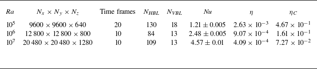


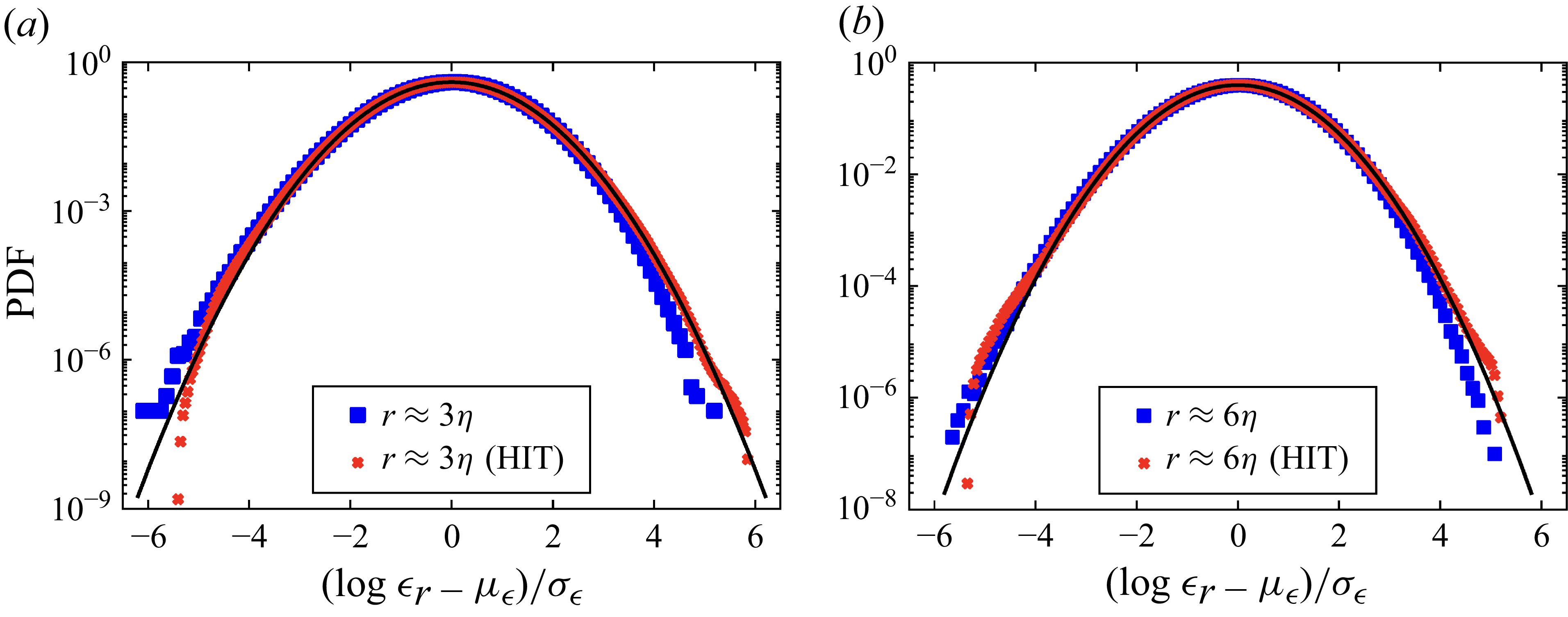


 Open access