







1. Introduction
The motion of particles in fluids depends on various factors, an important one being particle size. Sufficiently small particles almost perfectly follow the flow, while trajectories of larger particles deviate from fluid trajectories and may settle on preferential orbits. Related phenomena can be observed in various situations, ranging from the transport of dust and debris in hurricanes (Sapsis & Haller Reference Sapsis and Haller2009) over water purification (Seo, Lean & Kole Reference Seo, Lean and Kole2007) to biomedical applications such as blood cell coagulation and platelet aggregation (Leiderman & Fogelson Reference Leiderman and Fogelson2011). Another example is cell sorting and particle manipulation on the microscale using the flow over topography, which often consists of open cavities (Hur, Mach & Di Carlo Reference Hur, Mach and Di Carlo2011; Karimi, Yazdi & Ardekani Reference Karimi, Yazdi and Ardekani2013).
Most work has been devoted to spherical particles. In an unbounded fluid and when the particle Reynolds and Stokes numbers are small, the motion of a spherical particle can be described by the Maxey–Riley equation (Maxey & Riley Reference Maxey and Riley1983), which includes the Stokes drag, the effect of added mass, inertia, buoyancy, the Basset history term and Faxén's correction. A further simplification results from an expansion of the Maxey–Riley equation in terms of a small Stokes number leading to the so-called inertial equation (Lasheras & Tio Reference Lasheras and Tio1994; Haller & Sapsis Reference Haller and Sapsis2008) for the particle's velocity. At leading order in  ${\textit {St}}$, only inertia and buoyancy forces cause deviations from perfect advection of the particle.
For neutrally buoyant and finite-size particles, Babiano et al. (Reference Babiano, Cartwright, Piro and Provenzale2000) considered a variant of the Maxey–Riley equation including the inertial term and the Stokes drag. While neutrally buoyant particles initialised with a velocity equal to the flow velocity follow the flow perfectly, the particle trajectories must not be stable. Small deviations of the particle motion from that of the fluid can amplify exponentially, even if the particle has the same density as the fluid. This was demonstrated for a neutrally buoyant particle in a two-dimensional Taylor–Green flow, where the particle trajectory diverges exponentially from streamlines in flow regions with high strain rates and settles in regions where fluid rotation is dominant. For this pure particle-size effect to become operative, the Okubo–Weiss parameter  $Q$ must locally exceed $Q > 4/(9\,{\textit {St}}^2)$. Experimentally, Ouellette, O'Malley & Gollub (Reference Ouellette, O'Malley and Gollub2008) provided evidence for a size effect on the motion of nearly density-matched particles in a two-dimensional time-dependent chaotic flow. Apart from the pure size effect, Sapsis & Haller (Reference Sapsis and Haller2008) provided a rigorous criterion for weakly inertial particles to distinguish flow regions that attract or repel particles, and generalised the criterion to three-dimensional flow. Finally, in the presence of strong shear or when the particle Reynolds number is no longer small, the Maxey–Riley equation breaks down. Under such conditions, the inertia term of the flow perturbed by the presence of the particle needs to be taken into account. This causes lateral lift forces on the particle, resulting in a particle migration across the unperturbed streamlines (Saffman Reference Saffman1965; Asmolov Reference Asmolov1990; McLaughlin Reference McLaughlin1991).
When a particle is transported to a solid wall or a free surface, the Maxey–Riley equation cannot predict the particle motion correctly, because the presence of the boundary will largely modify the flow around the particle compared to the case of an unbounded fluid. The lateral migration and clustering of particles in pipe flow was first observed by Segré & Silberberg (Reference Segré and Silberberg1961, Reference Segré and Silberberg1962). The effect was initially attributed to shear-induced lift forces (Saffman Reference Saffman1965). Later, it was proven that the Segré–Silberberg phenomenon is caused by a combination of shear-induced lateral forces and a wall effect (Cox & Brenner Reference Cox and Brenner1968; Ho & Leal Reference Ho and Leal1974), because a particle moving parallel to a boundary experiences additional drag and lift forces. In the case when a particle is moving far away and perpendicularly towards a boundary, it is subject to a repulsive force due to the wall-normal gradient of the background flow (Rallabandi, Hilgenfeldt & Stone Reference Rallabandi, Hilgenfeldt and Stone2017; Li et al. Reference Li, Abbas, Morris, Climent and Magnaudet2020; Magnaudet & Abbas Reference Magnaudet and Abbas2021). Closer to the boundary, in a distance of the order of the particle size, the particle experiences strong lubrication forces in the wall-normal direction (Brenner Reference Brenner1961). As a result, in the near-wall region, the particle will lag behind the flow significantly. In the case where there is an additional component of fluid motion parallel to the boundary, the particle can migrate significantly across the streamlines. Such particle–boundary interaction due to the finite size of the particle can play an important role in the particle clustering in confined recirculating laminar flows, where particles have been found to be attracted to so-called finite-size coherent structures (FSCS; Romanò, Wu & Kuhlmann Reference Romanò, Wu and Kuhlmann2019b).
Finite-size coherent structures are frequently found in thermocapillary liquid bridges when the flow arises as a travelling hydrothermal wave (Wanschura et al. Reference Wanschura, Shevtsova, Kuhlmann and Rath1995). In this system, FSCS are also called particle accumulation structures (PAS; Schwabe, Hintz & Frank Reference Schwabe, Hintz and Frank1996). Tanaka et al. (Reference Tanaka, Kawamura, Ueno and Schwabe2006) found that initially well-mixed particles with appropriate size can accumulate rapidly on coherent structures. In the same flow system, Schwabe et al. (Reference Schwabe, Mizev, Udhayasankar and Tanaka2007) observed that neutrally buoyant particles are more rapidly attracted to PAS as compared to particles that are heavier or lighter than the fluid. Both experimental observations imply that the origin of such particle clustering is the finite size of the particles. Hofmann & Kuhlmann (Reference Hofmann and Kuhlmann2011) and Romanò & Kuhlmann (Reference Romanò and Kuhlmann2017) explained the rapid PAS formation by a collision of the particle with the free surface. In their model, this collision is inelastic in the direction normal to the interface. The mechanism is operative provided that the underlying flow exhibits chaotic and regular streamlines in some reference frame (the co-moving frame in the case of hydrothermal waves) and the regular streamlines in the Kolmogorov–Arnold–Moser (KAM) tori (Ottino Reference Ottino1989; Bajer Reference Bajer1994) of the incompressible flow approach the boundary closely. Repeated particle–boundary interaction can then rapidly transfer suitably-sized particles initially moving in the region of chaotic streamlines to a quasi-periodic trajectory closely resembling a KAM torus, or to a closed trajectory resembling a periodic streamline. While inertia due to the density difference between particle and fluid can also lead to periodic attractors, such inertial attraction is typically much slower in a hydrothermal wave in a liquid bridge than the attraction due to the particle–boundary effect (Muldoon & Kuhlmann Reference Muldoon and Kuhlmann2016; Romanò & Kuhlmann Reference Romanò and Kuhlmann2018). FSCS in thermocapillary liquid bridges have been reviewed by Romanò & Kuhlmann (Reference Romanò and Kuhlmann2019).
Finite-size coherent structures can also arise in cavity flows. Romanò, Kunchi Kannan & Kuhlmann (Reference Romanò, Kunchi Kannan and Kuhlmann2019a) simulated numerically the particle motion in an incompressible two-sided lid-driven cavity flow with chaotic and regular streamlines coexisting. Using a model based on lubrication theory (Brenner Reference Brenner1961; Breugem Reference Breugem2010) to describe the effect of the moving walls on a nearby particle, they found periodic or quasi-periodic particle attractors that resemble closely the structure of KAM tori of the background flow. For neutrally buoyant particles, Wu, Romanó & Kuhlmann (Reference Wu, Romanó and Kuhlmann2021) verified experimentally the existence of FSCS created by the particle–boundary interaction. They also demonstrated that the combined action of the wall effect, inertia effect and buoyancy can create attractors for weakly inertial particles that differ from those for neutrally buoyant particles. A related phenomenon is the creation of particle limit cycles in a two-dimensional vortex flow by centrifugal buoyancy that is balanced by a repulsion from the boundary (Romanò et al. Reference Romanò, Kuhlmann, Ishimura and Ueno2017). Furthermore, Haddadi & di Carlo (Reference Haddadi and di Carlo2017) found limit cycles for neutrally buoyant spheres in an open micro-cavity. The mechanism was explained as a combination of shear-induced migration and particle–boundary interaction.
Apart from the studies and flow systems mentioned, the effect of a three-dimensional confinement by impermeable boundaries on the motion of finite-size particles in an incompressible flow has not yet been fully understood. The above studies have indicated that non-trivial particle attractors in steady flows can be created by a confinement, in particular, in the presence of tangentially moving boundaries. Except for the spatially periodic flow system investigated by Wu et al. (Reference Wu, Romanó and Kuhlmann2021), the balance between inertia and confinement effects has not been analysed in detail for particles being attracted to limit cycles near a moving boundary. It is desirable, therefore, to better understand the interplay between inertia and confinement in a canonical flow system such as e.g. the lid-driven cube (Kuhlmann & Romanò Reference Kuhlmann and Romanò2019). On a macroscopic scale, the confinement effects are subtle, because inertia effects on the motion of small particles grow quadratically with the particle size and may easily dominate those caused by the presence of boundaries. On the other hand, confinement effects become dominant in micro systems. Since micro systems are not easily amenable to measurement, we investigate a generic macro system, the lid-driven cube, and consider neutrally and almost neutrally buoyant spherical particles to elucidate the roles of KAM tori in the flow, and inertia and buoyancy forces for the existence, shape and strength of attractors for the particle motion. Such knowledge is expected to enable better understanding of the particle dynamics in confined two- and three-dimensional flows in micro systems such as the creation of particle depletion zones (Orlishausen et al. Reference Orlishausen, Butzhammer, Schlotbohm, Zapf and Köhler2017) or the limit cycles in an open cavity flow (Haddadi & di Carlo Reference Haddadi and di Carlo2017). Also, the design of microscale particle handling systems like filtration platforms or cell separation devices should benefit from a more complete understanding of the underlying flow physics.
The flow in the iconic lid-driven cube has been investigated by many authors (e.g. De Vahl Davis & Mallinson Reference De Vahl Davis and Mallinson1976; Goda Reference Goda1979; Feldman & Gelfgat Reference Feldman and Gelfgat2010; Kuhlmann & Albensoeder Reference Kuhlmann and Albensoeder2014; Lopez et al. Reference Lopez, Welfert, Wu and Yalim2017). For reviews, see Shankar & Deshpande (Reference Shankar and Deshpande2000) and Kuhlmann & Romanò (Reference Kuhlmann and Romanò2019). Owing to its simplicity, this system provides an ideal test bed for studying particle motion in a steady three-dimensional flow. For a moderate Reynolds number  ${\textit {Re}}=UH/\nu$ (where $H$ is the cavity height) for which the flow is steady and three-dimensional, Tsorng et al. (Reference Tsorng, Capart, Lai and Young2006, Reference Tsorng, Capart, Lo, Lai and Young2008) have measured the motion of a macroscale spherical particle. Particles were found to settle on preferential trajectories. The phenomenon was explained in terms of shear-induced migration, but wall-induced forces were not taken into consideration. Furthermore, since the particle trajectory was not measured for a sufficiently long period of time, the final state of the particle motion was not fully revealed. More precise studies of the particle motion in the lid-driven cube are lacking. Numerical simulations of the flow in the lid-driven cube by Ishii, Ota & Adachi (Reference Ishii, Ota and Adachi2012) and Romanò, Türkbay & Kuhlmann (Reference Romanò, Türkbay and Kuhlmann2020) have shown the coexistence of chaotic streamlines with a large variety of KAM tori at moderate Reynolds numbers ranging from ${\textit {Re}}=100$ to $300$. The existence of these structures suggests that particle attractors due to the confinement may well exist in this system.
To put the interpretation of the motion of finite size particles in the lid-driven cube on more solid ground, we track experimentally the motion of neutrally buoyant and non-neutrally buoyant spherical particles for  ${\textit {Re}}=100$ and $200$, at which KAM tori are most abundant. The experimental set-up and the particle properties are described in § 2. In § 3, the numerical reconstructed topologies of the cavity flow are presented for the two Reynolds numbers. The key mechanisms by which particle attractors can be created are introduced in § 4, followed in § 5 by an explanation of the measurement procedure and the method of analysis of the particle trajectories. Measured particle trajectories for both neutrally buoyant and inertial particles with various radii and densities are presented and discussed in §§ 6 and 7 for ${\textit {Re}}=100$ and $200$, respectively. Finally, conclusions are drawn in § 8.
2. Experiment set-up
2.1. The lid-driven cavity
We target the motion of a Newtonian fluid and of a suspended particle in a cube, where the flow is driven by the tangential motion of one of its walls (the lid). Since a permanent and precise tangential motion of a plane wall over a cube requires a relatively complex hardware, the cubic geometry is approximated experimentally by a cuboidal cavity based on the apparatus used before by Siegmann-Hegerfeld (Reference Siegmann-Hegerfeld2010), Siegmann-Hegerfeld, Albensoeder & Kuhlmann (Reference Siegmann-Hegerfeld, Albensoeder and Kuhlmann2008, Reference Siegmann-Hegerfeld, Albensoeder and Kuhlmann2013) and Wu et al. (Reference Wu, Romanó and Kuhlmann2021). In this set-up, sketched in figure 1, two of the facing lateral walls of the cube are realised by independently rotating stainless steel cylinders of radius  $R=135$ mm, large compared to the cavity height $H=40.5$ mm. The maximum and minimum horizontal distances between the two parallel cylinder are $W_{max}=41.9$ mm and $W_{min}=38.9$ mm, respectively, yielding an algebraic mean distance $\bar {W}=40.4$ mm. The top, bottom and lateral side walls are made from Plexiglas. To convert the previous set-up into a cuboidal geometry, the length in the spanwise direction has been fixed at $L = 40.0$ mm by mounting a correspondingly machined Plexiglas block into the originally spanwise extended cavity. These dimensions yield a nearly cubic cavity with aspect ratios $\varGamma =\bar {W}/H=0.998$ and $\varLambda =L/H=0.988$.
Sketch of the cavity (solid lines) with coordinates and dimensions. Two facing side walls are curved and realised by large cylinders. The cylinder located at  $x<0$ is stationary, while the cylinder at $x>0$ rotates with constant angular velocity $\varOmega$. The wall curvature ( $R^{-1}$) is shown exaggerated. The origin of the coordinate system is placed in the centre point of the cavity. The acceleration due to gravity $\boldsymbol g$ acts in the negative $y$ direction.
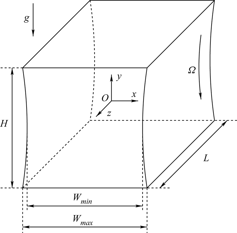
We consider the case in which one cylinder is kept at rest. The other cylinder is rotating with surface velocity  $\varOmega R$, where $\varOmega$ is the angular velocity of the cylinder, driving the fluid motion. The working fluid is Bayer silicon oil M20 with kinematic viscosity $\nu =20$ cSt and density $\rho _f=0.95\,{\rm g}\,{\rm cm}^{-3}$ at $20\,^{\circ }{\rm C}$. The dependence of the kinematic viscosity on the temperature has been measured by Wu et al. (Reference Wu, Romanó and Kuhlmann2021) and was fitted by
 \begin{equation} \frac{\nu}{\text{cSt}} = 31.6717 - 0.5976 \times \frac{T}{^\circ\text{C}} + 0.0044\times \left(\frac{T}{^\circ\text{C}}\right)^2. \end{equation}
Since the viscosity depends on the temperature, the temperature of the fluid is measured every 5 s by two resistance temperature devices of type PT1000, and the rotation speed of the cylinder  $\varOmega$ is adjusted in order to keep the Reynolds number ${\textit {Re}} = \varOmega R H/\nu (T)$ constant during the measurements. In order to control the temperature and keep it homogeneous, the cavity including the two cylinders is immersed in a larger container filled with the same fluid. The fluid in the outer bath is recirculated through a thermostat that can maintain the temperature at a specific value with a tolerance of $\pm 0.1\,^\circ$C. To facilitate optical access, the top wall of the cavity as well as one side wall at $z=L/2$ are not immersed in the temperature bath. For further details on the apparatus, we refer to Siegmann-Hegerfeld (Reference Siegmann-Hegerfeld2010) and Wu et al. (Reference Wu, Romanó and Kuhlmann2021).
2.2. Suspended particles
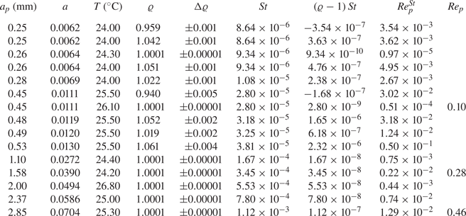
The fluid in the cavity is seeded with a single spherical particle made from polyethylene. Different particle radii are considered in the range  $a_p\in [0.25, 2.86]$ mm. Apart from the particle size, the particle-to-fluid density ratio $\varrho = \rho _p/\rho _f$ is of key importance. The fluid density $\rho _f(T)= [0.97891 - 0.0010184 \times (T/^\circ \text {C})]$ g cm $^{-3}$ was obtained by linear approximation of the discrete data at $[0, 25, 50]\, ^\circ \text {C}$ specified by the manufacturer (see also Wu et al. Reference Wu, Romanó and Kuhlmann2021). Due to the error in the temperature, this leads to a relative uncertainty of $\Delta \rho _f/\rho _f \approx \pm 0.0001$ for the fluid density. The density of the particle $\rho _p$ is varied such that the density ratio ranges in $\varrho \in [0.94, 1.06]$. Neutrally buoyant particles have been realised by adjusting the fluid temperature. In a separate experiment with a better temperature control of $\pm 0.01\,^\circ$C, the relative density $\varrho$ of the particles was determined by measuring settling velocity. The properties of the particles used are specified in table 1. Note that while the density for particles with $\varrho =1.0001$ could be determined with accuracy $\Delta \varrho =\pm 0.00001$ in the settling experiment, the accuracy of $\varrho$ in the cavity experiments was reduced to $\pm 0.0001$, owing to the less accurate temperature control.
Particle radius  $a_p$, non-dimensional particle radius $a=a_p/H$, operating temperature $T$, and particle-to-fluid density ratio $\varrho =\rho _p/\rho _f$ determined by measuring the settling velocity in the quiescent fluid of temperature $T$, error $\Delta \varrho$, and ${\textit {St}}=2a^2/9$. Note that the error $\Delta \varrho$ made in this process is smaller here due to the better temperature control up to $\pm 0.01\,^{\circ }{\rm C}$. Also provided are the inertial factor $(\varrho -1)\,{\textit {St}}$, the particle Reynolds number ${\textit {Re}}_p^{St}=a_pV_{Stokes}/\nu$ based on the Stokes settling velocity, and the particle Reynolds number ${\textit {Re}}_p=a_p\,\overline {V_{slip}}/\nu$ based on the average slip velocity $\overline {V_{slip}}=\overline {|\boldsymbol {u} - \dot {\boldsymbol {X}}|}$ at ${\textit {Re}}=200$.
To determine precisely the trajectory of the particle inside the cuboidal cavity, it is illuminated by a halogen lamp and the particle motion is recorded by two synchronised cameras (FLIR Grasshopper, model GS3-U3-32S4M-C), one equipped with a NIKKOR 24 mm f/2.8D lens and the other with a NIKKOR 35 mm f/2.0D lens. The sampling frequency is 20 Hz. The cameras view the interior of the cavity in the  $y$ and $z$ directions, respectively, through the plane side and top walls, both of which are made from transparent Plexiglas. The side wall at $z=-L/2$ and the bottom wall at $y=-H/2$ are made from black Plexiglas to provide a black background for both cameras. During post-processing of the recorded movies, the centroid of the particle is determined for each frame of each camera. This is accomplished essentially by application of the Laplacian of a Gaussian filter after which the position of the centroid is identified by the local brightness maximum. After obtaining the two-dimensional position of the particle's centroid in the sensor plane of each camera, the three-dimensional coordinate of the particle relative to the cavity can be found by a triangulation process that also takes into account the refractive index variations at the interfaces between air, Plexiglas and silicone oil, based on Snell's law. The details of the algorithm can be found in Wu et al. (Reference Wu, Romanó and Kuhlmann2021).
In the following, we will frequently use non-dimensional quantities based on the length scale  $H$, the viscous time scale $t_\nu = H^2/\nu(T)\approx 80$ s, which is temperature dependent, and the viscous velocity scale $\nu (T)/H$. If required, the temperature of the fluid is specified. A table of the properties of the particles employed and the fluid temperatures at which they were tracked is provided in table 1.
3. Flow field without particles: flow topology
The flow in a cubic or cuboidal cavity is three-dimensional for all Reynolds numbers (Kuhlmann & Romanò Reference Kuhlmann and Romanò2019). Moreover, the flow in a lid-driven cube is steady for  ${\textit {Re}} < 1906$ (Kuhlmann & Albensoeder Reference Kuhlmann and Albensoeder2014), and for Reynolds numbers ${\textit {Re}}=100$, 200 and 300, chaotic and regular streamlines in the form of KAM tori coexist (Ishii & Adachi Reference Ishii and Adachi2010; Romanò et al. Reference Romanò, Türkbay and Kuhlmann2020).
The steady flow in the present cuboidal cavity differs slightly from the flow in a lid-driven cube due to the presence of the curved walls. The wall curvature has little effect on the gross flow structure and on the major KAM structures. However, the finer KAM structures differ between the cases. Therefore, we carried out numerical simulations of the flow in the cuboidal cavity with NEK5000, and analysed the streamline structure using the same criteria and methodology as in Romanò, des Boscs & Kuhlmann (Reference Romanò, des Boscs and Kuhlmann2020) for the cubic cavity. Accordingly, we employ 20 Legendre–Gauss–Lobatto spectral elements of 7th degree per space direction, resulting in a total of approximately 4 million spectral points. To discretise the Navier–Stokes and continuity equations, we employ a spectral interpolation consistent with degree 7 in  $x$,
$x$,  $y$ and $z$. After having computed the steady flow, the same Runge–Kutta Dormand–Prince method (Dormand & Prince Reference Dormand and Prince1980) as in Romanò et al. (Reference Romanò, des Boscs and Kuhlmann2020) is employed to compute streamlines by integrating the trajectories of individual fluid elements with absolute and relative tolerances of $10^{-7}$. From these streamlines in the form of a sequence of discrete points, a Poincaré section is obtained as the set of intersection points of the streamline with a plane surface given by a specific coordinate value. From many such Poincaré sections, the KAM tori can be reconstructed as three-dimensional toroidal surfaces as described in Romanò et al. (Reference Romanò, des Boscs and Kuhlmann2020).
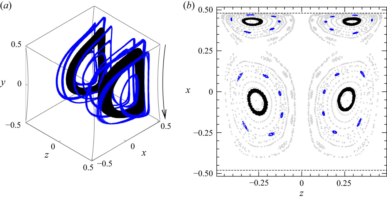
The flow topology in the present cuboidal cavity for  ${\textit {Re}}=100$ and $200$ is interesting, because of the complex structure of the more slender KAM tori. For both Reynolds numbers, the flow is reflection symmetric with respect to the midplane $z=0$. Figure 2(a) shows a three-dimensional view of the KAM tori for ${\textit {Re}}=100$, whose structure can be better seen in the Poincaré section at $y=0$ (figure 2b) with cross section $(x,z)\in [-0.48125,0.48125] \times [-0.5, 0.5]$. The topology is dominated by two mirror-symmetric sets of KAM tori with period one (light grey) surrounded by chaotic streamlines (not shown). Inside these period-one sets of tori (figure 2b), we find two layers of chaotic streamlines (not shown) within which slender KAM tori of higher period – six (green) and seven (dark grey) – are embedded. These tori with higher periodicity must have been created by a 1 : 6 and a 1 : 7 resonance, respectively. The two chaotic layers with embedded higher-order KAM tori are sealed by the contiguous KAM tori of $T_1$ and by thin layers of period-one KAM tori denoted $S_A$ and $S_B$. In figure 2(a), the outermost sealing layers of period-one tori ( $S_A,S_B$) have been omitted to show $T_6$ (green) and $T_7$ (dark grey/black).
Numerically calculated KAM tori for  ${\textit {Re}} = 100$. (a) Three-dimensional view of the innermost KAM tori of period one (light grey), surrounded by the largest reconstructible KAM tori of period six (green) and period seven (dark grey). The lid motion is indicated by an arrow. (b) Poincaré section on $y=0$ of quasi-periodic streamlines on the KAM tori shown in (a). The KAM tori $S_A$ and $S_B$ represent transport barriers to the chaotic streamlines (not shown) surrounding the KAM tori $T_6$ and $T_7$. The dashed lines indicate the boundary of the domain in the plane shown.
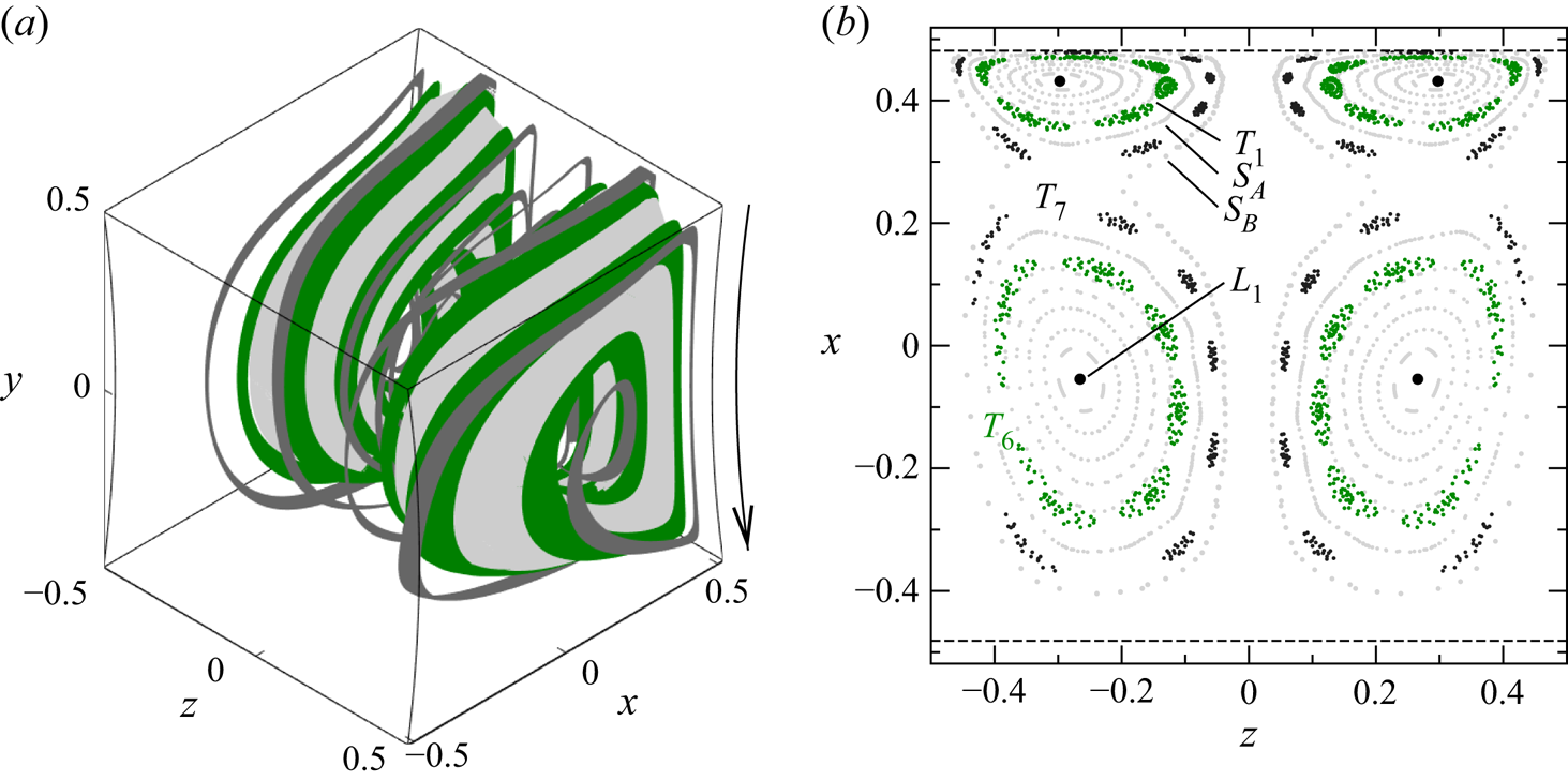
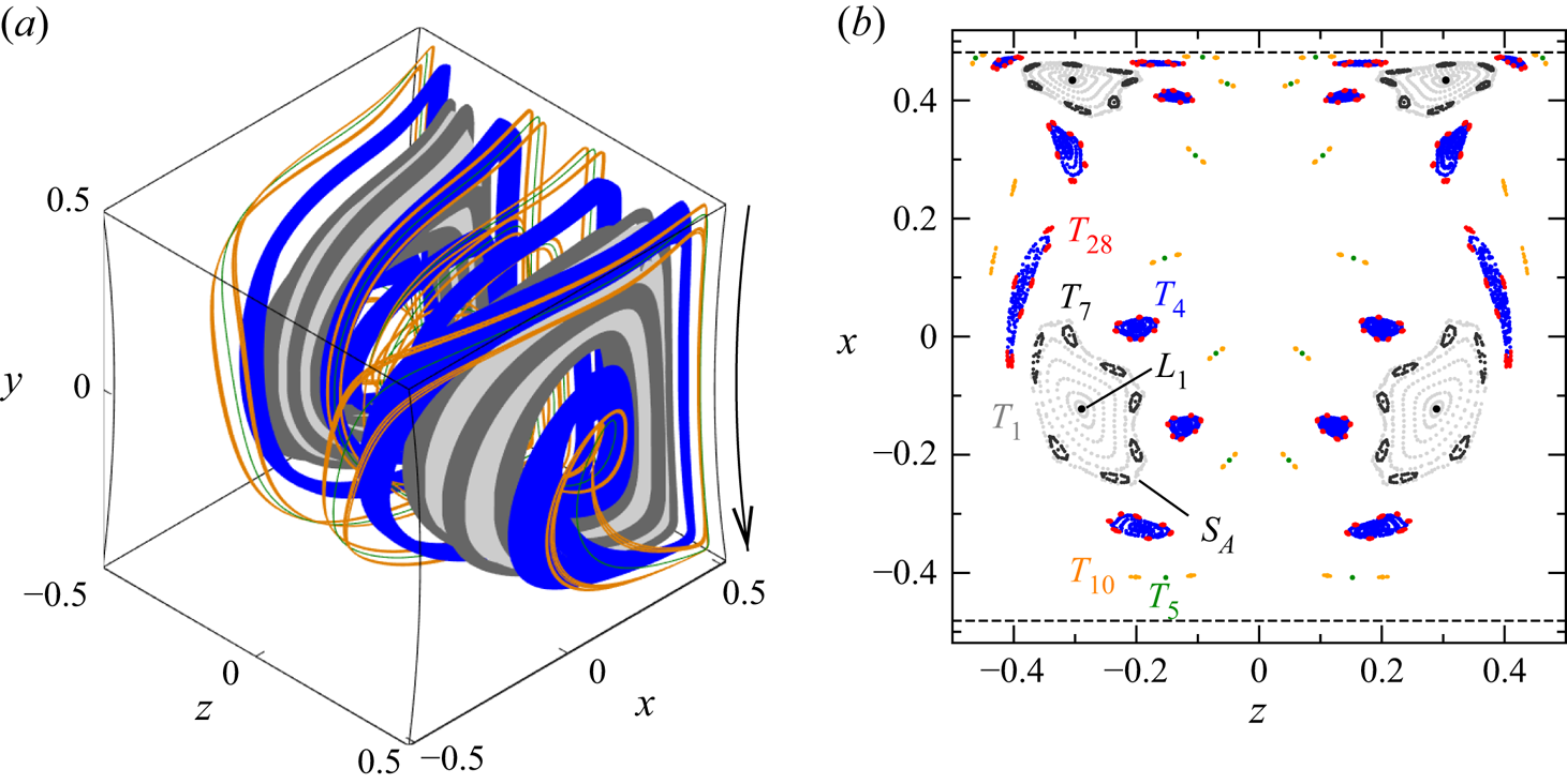
Figure 3 illustrates the KAM tori for  ${\textit {Re}}=200$ with a three-dimensional view shown in figure 3(a). The topology has become more complex, and the main KAM tori $T_1$ of period one (light grey) have shrunk at the expense of the chaotic region. As for ${\textit {Re}}=100$, we also find secondary tori $T_7$ of period seven (dark grey/black), embedded in a thin chaotic layer between the outermost tori of $T_1$, best seen in figure 3(b). The thin chaotic layer is separated from the outer chaotic region by a transport barrier $S_A$ (shown only in figure 3b). In addition, we find in the outer chaotic sea a secondary KAM torus $T_4$ of period four (blue), which is closely surrounded by another system of tori $T_{4\times 7}$ (red), which closes after a total of 28 revolutions about $T_1$. Further, we identify a slender KAM torus $T_5$ (green) of period five, of which only four returns are visible in figure 3(b) due to the location of the Poincaré section at $y=0$. For the same reason, the slender KAM torus $T_{5\times 2}$ (orange) of period ten that winds around $T_5$ exhibits only nine returns in the Poincaré plane $y=0$.
Numerically calculated KAM tori for  ${\textit {Re}} = 200$. (a) Three-dimensional view of the largest reconstructible KAM tori $T_1$ (light grey), $T_7$ (dark grey), $T_4$ (blue), $T_5$ (green) and $T_{10}$ (orange). The arrow indicates the direction of the lid motion. (b) Poincaré section on $y=0$ of quasi-periodic streamlines on the KAM tori shown in (a). In addition, the KAM tori $T_{4\times 7}$ (red) can be identified. The dashed lines indicate the boundary of the domain in the plane shown.
For both Reynolds numbers, we find that all KAM tori approach the moving wall closely, separated from the lid only by a thin layer of chaotic streamlines. According to Hofmann & Kuhlmann (Reference Hofmann and Kuhlmann2011), Romanò & Kuhlmann (Reference Romanò and Kuhlmann2017) and Barmak, Romanò & Kuhlmann (Reference Barmak, Romanò and Kuhlmann2021), such a situation can promote the creation of stable limit cycles for suspended particles with  $\varrho = 1$, i.e. for particles that tend to move similarly to the fluid in the absence of particles. The attractors are created by a localised particle–wall interaction that is communicated by lubrication forces and must be distinguished from attractors created by inertia when $\varrho \ne 1$ (Romanò et al. Reference Romanò, Kunchi Kannan and Kuhlmann2019a). Even though the former attractors rely on KAM tori located at a distance from the wall comparable to the particle size, we will often call the localised particle–wall interaction simply the wall effect. Although this wall effect depends on the particle size, it differs from a size effect in the bulk (e.g. the Faxén correction).
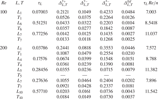
The existence of such attractors has already been demonstrated by Wu et al. (Reference Wu, Romanó and Kuhlmann2021), who investigated particle motion attractors in a steady periodic cellular flow in a cavity extended in the  $z$ direction and driven by an opposing motion of the two facing walls. In the following, we inquire into the existence of particle motion attractors in the present cuboidal cavity flow. The cuboidal flow differs from the periodic flow investigated by Wu et al. (Reference Wu, Romanó and Kuhlmann2021) by the characteristic end wall effect, which causes the three-dimensionality of the flow. The existence and location of particle motion attractors depend on the location of the KAM tori relative to the boundaries. Therefore, the characteristic properties of the main numerically computed KAM tori of interest are collected in table 2, providing the minimum distances $\varDelta _\psi$ of the central closed streamline and the minimum distances $\varDelta _T$ of the largest reconstructible KAM tori from the top and bottom walls (superscripts ‘ $y_+$’ and ‘ $y_-$’, respectively) and from the two curved walls (superscripts ‘ $x_-$’ and ‘lid’). In addition, the orbit time $\tau _L$ of the closed streamline is provided in units of the viscous diffusion time, i.e. $\tau _L = t_L/t_\nu$. Obviously, the closed streamlines and tori always approach the moving wall (superscript ‘lid’) the closest. The torus $T_5$ for ${\textit {Re}}=200$ is so slender that we did not distinguish it from its closed streamline.
Numerically computed properties of the largest reconstructible KAM tori ( $T$) and closed streamlines ( $L$). Specified are the period $\tau _L$ of the closed streamline and the minimum distances of the closed streamline ( $\varDelta _L$) and KAM tori ( $\varDelta _T$) from the boundaries. The superscript indicates the boundary to which the distance relates: $y_+$ for $y=0.5$; $y_-$ for $y=-0.5$; $x_-$ for the curved wall at $x<0$; lid for the moving curved wall at $x>0$. Also given is the mean time for a single turnover in convective scaling $\tau _L\,{\textit {Re}}/n$, where $n$ is the period of the orbit.
4. Key factors influencing the particle motion
Particles that have nearly the same density as the fluid are mainly advected. Since attractors for exactly advected particles are impossible, deviations from pure particle advection are necessary for attractors to exit. Three main factors contribute to the formation of attractors in steady three-dimensional closed flows.
One such factor is the repulsive action on the particle caused by the boundaries, in particular the moving wall. This effect becomes prominent if other forces like inertia and buoyancy are absent. Hofmann & Kuhlmann (Reference Hofmann and Kuhlmann2011) have shown that stable limit cycles for the particle motion can be created by the repulsion of tangentially moving boundaries, if the closed streamline of a KAM torus approaches the moving boundary closer than the centroid of a spherical particle can do. The resulting limit cycle is a trajectory on a KAM torus in the bulk that is closed by a relatively short segment near the boundary within which the boundary effect is acting. This effect is very important in thermocapillary flows (Muldoon & Kuhlmann Reference Muldoon and Kuhlmann2016; Barmak et al. Reference Barmak, Romanò and Kuhlmann2021), for which various particle motion attractors have been observed (Schwabe et al. Reference Schwabe, Mizev, Udhayasankar and Tanaka2007, see e.g.). Romanò & Kuhlmann (Reference Romanò and Kuhlmann2017) have pointed out that the onset criterion of Hofmann & Kuhlmann (Reference Hofmann and Kuhlmann2011) must be modified if lubrication forces between particle and boundary are taken into account. The existence of limit cycles due to the boundary effect can be understood in terms of a localised dissipation that is introduced in the dynamical system governing the particle motion. The boundary-induced limit cycles are stable (Hofmann & Kuhlmann Reference Hofmann and Kuhlmann2011).
The other important factors are buoyancy and inertia, both caused by a density mismatch between particle and fluid. Inertia forces also introduce a dissipation in the dynamical system for the particle motion, thus allowing for limit cycles to exist. Different from the boundary effect, however, the particle limit cycles caused by particle inertia in a flow that is steady in the absence of the particle can be either stable or unstable. While buoyancy forces alone cannot lead to attractors, because they derive from a potential (see also Sapsis & Haller Reference Sapsis and Haller2010), they can determine the stability of the inertia-induced limit cycles (Wu et al. Reference Wu, Romanó and Kuhlmann2021) and boundary-induced attractors (Romanò, des Boscs & Kuhlmann Reference Romanò, des Boscs and Kuhlmann2021).
Using the above-mentioned diffusive scaling for a fluid with constant properties, the motion of a small particle with radius  $a=a_{p}/H$ sufficiently far from the boundary can be modelled, to first order in $a^2$, by the inertial equation (Lasheras & Tio Reference Lasheras and Tio1994)
 \begin{equation} \dot{\boldsymbol X} = \boldsymbol u -(\varrho-1)\, {\textit{St}} \left(\frac{\mathrm{D} \boldsymbol u}{\mathrm{D} \tau} + \frac{\boldsymbol e_y}{ {\textit{Fr}}^2}\right), \end{equation}
where  $\boldsymbol X(\tau )$ is the trajectory of the particle, $\tau$ is the dimensionless time, $\boldsymbol u = u\boldsymbol e_x + v\boldsymbol e_y + w\boldsymbol e_z$ is the flow field expressed in Cartesian components ( $\boldsymbol e_x$, $\boldsymbol e_y$ and $\boldsymbol e_z$ are the unit vectors in the coordinate directions; see figure 1), ${\textit {St}} = 2a^2/9$ is the Stokes number, ${\textit {Fr}}=\sqrt {\nu ^2/(gH^3)}$ is the diffusively scaled Froude number, and $\mathrm {D}/\mathrm {D} t$ is the material derivative following the flow. For the present steady flow, $\mathrm {D}/\mathrm {D} \tau =\boldsymbol u\boldsymbol {\cdot }\boldsymbol {\nabla } \boldsymbol u$. From (4.1), to leading order in $a$, both buoyancy and inertia effects scale with $(\varrho -1)\,{\textit {St}}$.
In pure advection with  $\dot {\boldsymbol X}(\tau )=\boldsymbol u$, a particle can move on a KAM torus just like a fluid element. This particle motion is, however, structurally unstable: a weak inertial effect $(\varrho -1)\,{\textit {St}}\ll 1$ destroys the KAM structure of the particle's trajectory. In particular, the neutrally stable periodic particle orbit on the closed streamline in the case of advection becomes a stable or an unstable limit cycle. The stability property of the resulting limit cycle depends on the topological properties of the flow field, the sign of $\varrho -1$, and the strength and orientation of the buoyancy force. It is interesting to note that for constant Reynolds number, the relative importance of inertia to buoyancy forces remains constant. The squared inverse Froude number evaluated for the nominal viscosity 20 cSt amounts to ${\textit {Fr}}^{-2}=gH^3/\nu ^2 = 1.63\times 10^6$. The related Stokes number based on the settling velocity can be obtained easily by multiplication with $(\varrho -1)\,{\textit {St}}$ (see table 1).
From these considerations, inertia-induced limit cycles can be expected to form near closed streamlines, i.e. near the centres of KAM tori. In the two-sided lid-driven cavity investigated by Wu et al. (Reference Wu, Romanó and Kuhlmann2021), the KAM tori arise in periodic pairs. The two main tori existing in a single convection cell were located point symmetrically to each other with respect to the cell centre. Due to this symmetry and the direction of the gravity vector in their experiment, the effect of gravity on a particle moving in one of the two main tori was exactly opposite to the effect of gravity on a particle moving in the point-symmetrically located torus. As a result of buoyancy, the equivalence of the inertia-induced attractors near the two closed streamlines was found to be destroyed such that one of the two attractors even turned into a repeller (Wu et al. Reference Wu, Romanó and Kuhlmann2021). In the present lid-driven cuboid, the KAM tori arise in reflection-symmetric pairs such that the inertial-buoyant action on a moving particle is equivalent for both tori. Therefore, it is expected to find in the present system either two inertial-buoyant attractors or two inertial-buoyant repellers.
5. Experimental procedure and analysis of measured trajectories
The motion of a single spherical particle with non-dimensional particle radius  $a$ and relative density $\varrho$ in the cavity is measured for ${\textit {Re}}=100$ and $200$ following the procedures described in Wu et al. (Reference Wu, Romanó and Kuhlmann2021). In short, after the particle has been placed in the cavity, the flow is ramped up linearly at rate $\Delta {\textit {Re}}/\Delta t = 1000$ s $^{-1}$ and driven at ${\textit {Re}}=400$ for one minute. Since the flow is transient and the steady flow at ${\textit {Re}}=400$ in the cuboidal cavity exhibits only chaotic streamlines, as in the cubic cavity (Ishii et al. Reference Ishii, Ota and Adachi2012; Romanò et al. Reference Romanò, des Boscs and Kuhlmann2020), this initial phase randomises the position of the particle. Thereafter, the Reynolds number is ramped down at the same rate as the ramp-up until the targeted Reynolds number is reached. From this instant, which defines $t= \tau = 0$, the Reynolds number is kept constant at ${\textit {Re}}=100$ or $200$, and the particle motion is recorded.
Particles with different sizes and densities are considered (table 1). To study the pure geometrical confinement effect on the particle motion, the trajectories of small particles with density  $\varrho =1.0001$ almost matched to that of the fluid are measured. By varying the density ratio $\varrho$, the relative importance of inertia and buoyancy compared to the confinement effect can be assessed. In order to prove reproducibility of the recorded data and to arrive at statistically reliable results, each experiment is repeated several times. Of particular interest are the shapes of the attracting orbits and the rate of attraction. Following Wu et al. (Reference Wu, Romanó and Kuhlmann2021), the temporal evolution is monitored in the Poincaré plane defined by $y=0$. Provided that the asymptotic state is a limit cycle, the distance
 \begin{equation} d_n=[(x_n-x^*)^2 + (z_n-z^*)^2]^{1/2} \end{equation}
between each Poincaré point  $(x_n, z_n)$ of the particle's trajectory and the fixed point $(x^*, z^*)$ corresponding to the limit cycle is measured as a function of time $\tau _n$, where $n$ enumerates successive Poincaré points. In the case where the attractor is quasi-periodic, $(x^*, z^*)$ is defined as the geometric centre
 \begin{equation} (x^*,z^*)= \frac{1}{K} \sum_{k=N_{max}-K+1}^{N_{max}} (x_k,z_k) \end{equation}
of the last  $K$ Poincaré points, where $N_{max}$ is the total number of Poincaré points registered. Here, we use $K=20$.
The rate of attraction is also determined from  $d_n$. To that end, only Poincaré points in the plane $y=0$ are taken into account, which have approached the attractor closely, satisfying $d_n < d^* = 0.15$. The time it takes to satisfy this condition is called the initial transient time $\tau _I = \min \{\tau ' \mid \forall_{\tau >\tau '}\ d_n(\tau ) < d^*\}$. The decay function
 \begin{equation} d(\tau)=A\,\mathrm{e}^{-\sigma (\tau-\tau_I)} + B \end{equation}
is then fitted by least squares to the sequence of distances  $d_n$ to obtain the constants $A$ and $B$, and the attraction rate $\sigma$. Ideally, $B=0$ for a periodic attractor, while $B > 0$ for a quasi-periodic attractor. Experimentally, however, $B > 0$ always, because of small measurement errors in the positive distance function ( $d_n \ge 0$), even for a periodic orbit.
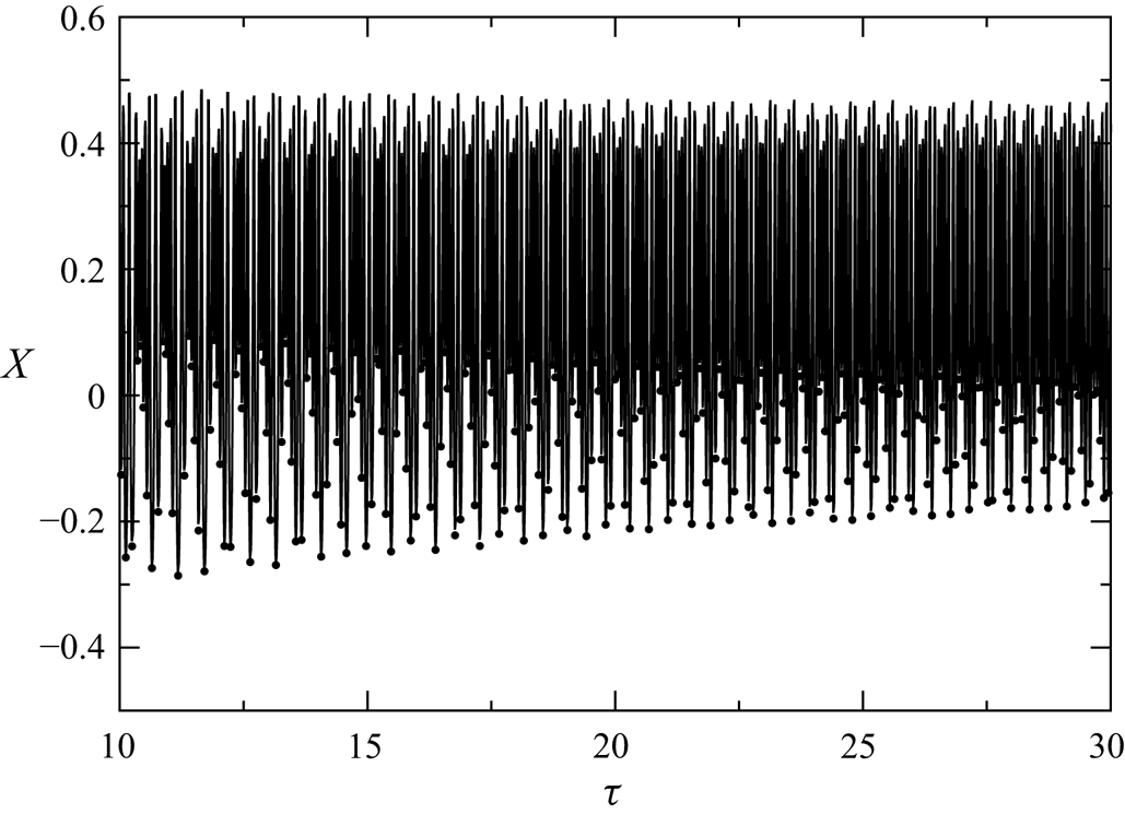
Alternatively, the asymptotic attraction rate to a periodic orbit or to a slender torus can be determined by monitoring the extremum values of any coordinate of the trajectory. An example is shown in figure 4. Here, the minima of  $X$ (dots) vary in a certain range. From the upper and lower envelopes of the minima, the attraction rate(s) and the asymptotic values for $\tau \to \infty$ can be obtained. A persistent variation of the minima indicates a toroidal motion, while the motion is periodic if the upper and lower envelopes converge to the same value for $\tau \to \infty$.
Example for the coordinate  $X(\tau )$ of a trajectory (line) and the local minima (dots) for ${\textit {Re}}=100$, $a=0.0064$ and $\varrho =1.0001$.
6. Results for  ${\textit {Re}}=100$

6.1. Motion of nearly neutrally buoyant particles
To target attractors for the particle motion that are caused mainly by particle–wall interaction, any inertia effects must be minimised. Therefore, we first consider particles whose density is nearly matched to that of the fluid. Nearly neutrally buoyant conditions were realised by adjusting the temperature of the fluid in the cavity experiment, yielding relative density  $\varrho =1.0001\pm 0.0001$ for all particles considered in this section, i.e. for particles with sizes $a = 0.0064$, 0.0111, 0.0272, 0.0390, 0.0494, 0.0586 and 0.0703. Their motion is considered for ${\textit {Re}} = 100$.
6.1.1. Limit cycles of period one
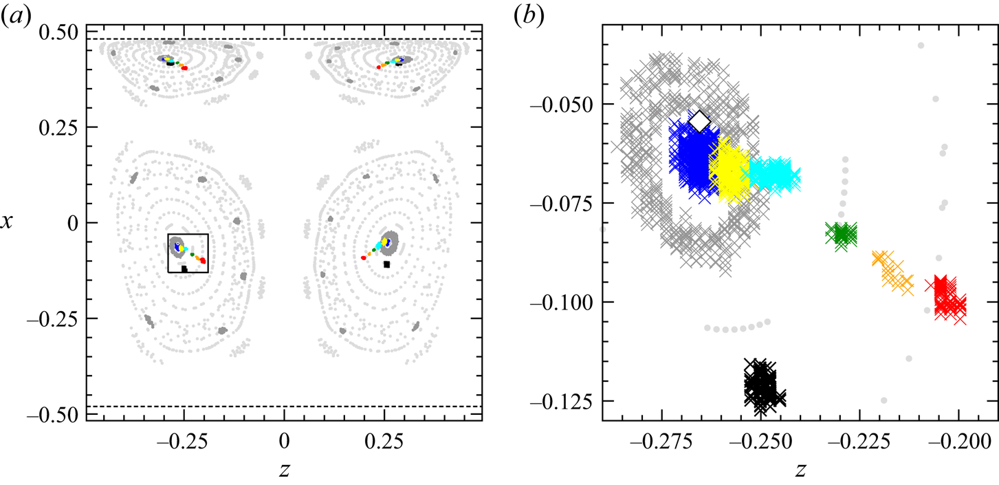
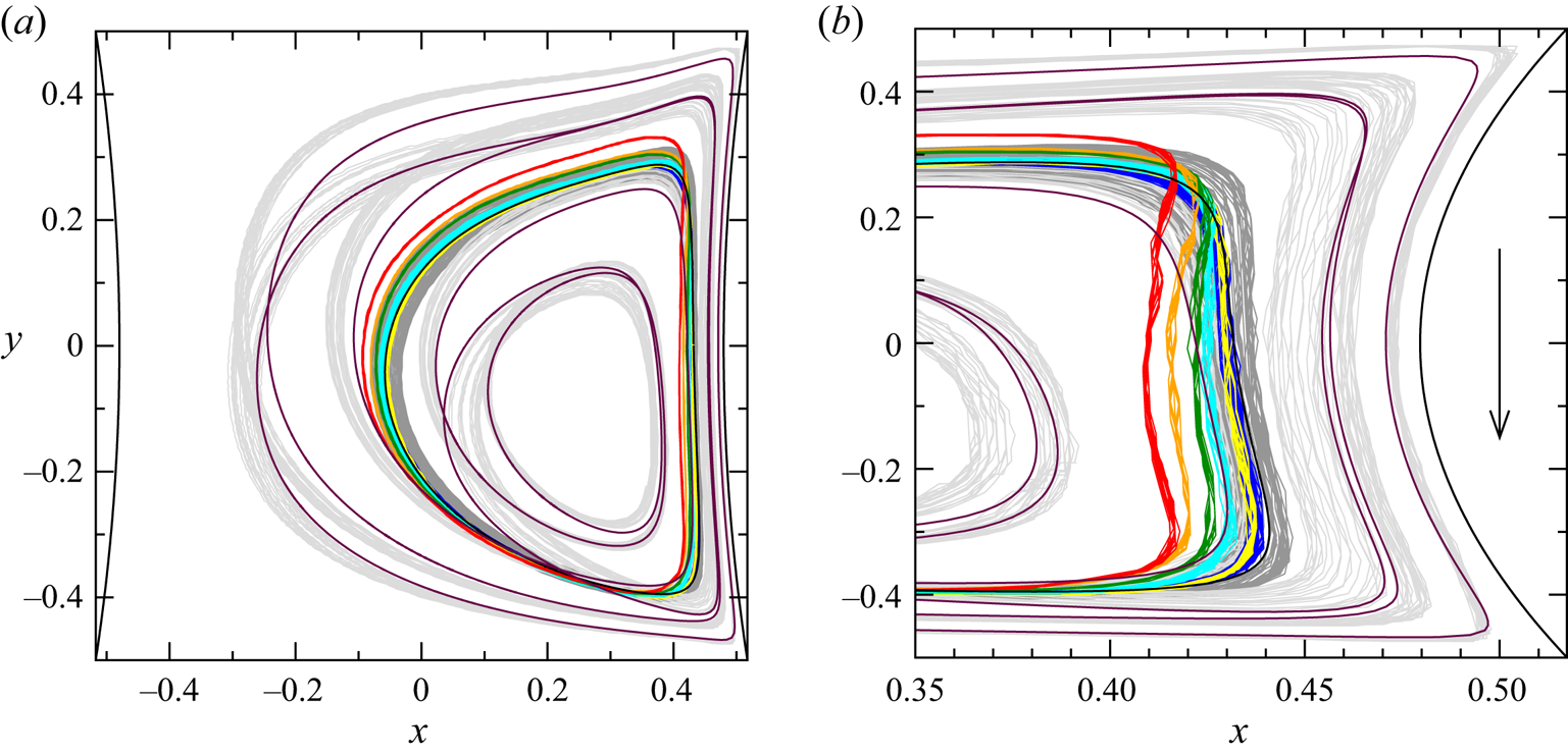
For  $\varrho = 1.0001$, we find a periodic attractor with period one in very close vicinity of the closed streamline $L_1$ for all particle sizes mentioned above. Figure 5 shows the locations of the limit cycles in the Poincaré plane $y=0$ (here and in the following, the dashed lines indicate the location of the curved walls in this plane). As can be seen, the attractors arise as mirror symmetric pairs and they grow out of the closed streamline (white diamond in figure 5b) as the particle size (coded by colour) increases from $a=0.0111$. With increasing $a$, the attractors move away from the moving wall in the $y=0$ plane, and closer to the symmetry plane $z=0$. The growth of the distance from the moving wall with increasing particle size is also seen in the projections of the limit cycles onto the $(x,y)$ plane shown in figure 6. In addition, the periodic orbits extend slightly further in the positive $y$ direction as $a$ increases. The Poincaré points for the smallest particle with $a=0.0064$ – corresponding to the dark grey crosses in figure 5(b) – near the closed streamline belong to a transient state at $t\in [6700,7200]$ s, which finally converges to a limit cycle for much longer time (see figure 19(b) below).
(a) Poincaré section on  $y=0$ of trajectories of nearly neutrally buoyant spherical particles ( $\varrho =1.0001$) on their respective attractors (colours). The colour indicates the particle radius $a$:
$a$:  $0.0064$ dark grey, 0.0111 blue, 0.0272 yellow, 0.0390 cyan, 0.0494 green, 0.0586 orange, and 0.0704 red. For comparison, the Poincaré section of KAM tori and closed streamlines are shown as light grey dots. The black dots represent the Poincaré section of the attractors for an inertial particle with $a=0.0119$ and $\varrho =1.052$. The large square indicates the zoom shown in (b), where attractors are shown by crosses and streamlines on KAM tori by light grey dots. The dashed lines indicate the boundary of the domain in the plane shown.
(a) Projection of all trajectories onto the  $(x,y)$ plane of nearly neutrally buoyant spherical particles ( $\varrho =1.0001$) moving on their respective attractors. The colour indicates the particle radius $a$:
$a$:  $0.0064$ light grey and dark grey, 0.0111 blue, 0.0272 yellow, 0.0390 cyan, 0.0494 green, 0.0586 orange, and 0.0704 red. Black and maroon lines indicate numerically computed closed streamlines of periods one and six, respectively. (b) Zoom, the x and y axes are scaled differently.
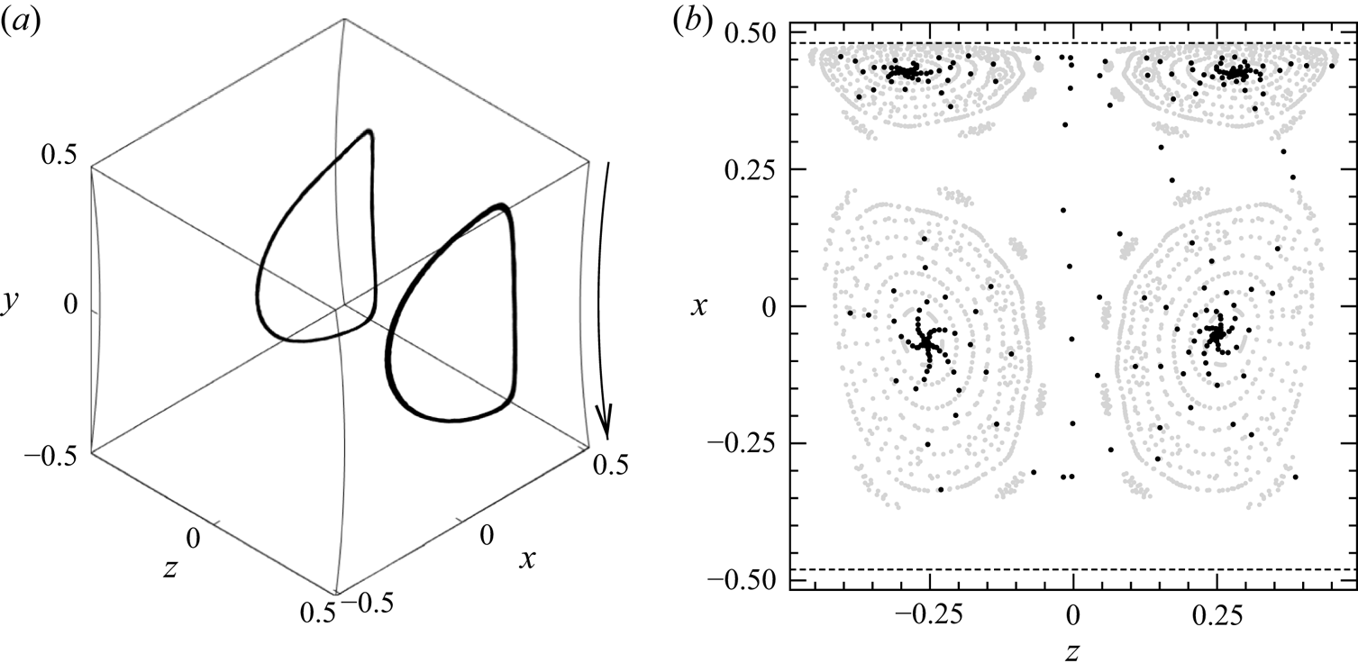
As a typical example, we consider in more detail the trajectory of a particle with  $a=0.0272$ and $\varrho =1.0001$. Initially, the particle is transferred by the boundary repulsion effect to one of the regions occupied by the two main sets of KAM tori $T_1$ of the flow. There, the particle approximately moves on KAM tori, but slowly spirals into the limit cycle. A three-dimensional view of the resulting limit cycle is shown in figure 7(a), where 40 trajectories have been superimposed. The close agreement of the trajectories demonstrates the reproducibility of the two limit cycles. Figure 7(b) shows all Poincaré points for two realisations. It is seen that during the asymptotic transient motion, the trajectories are characterised by two incommensurate frequencies whose ratio is close to five.
(a) Forty trajectories for  $a=0.0272$ ( $a_{p}=1.1$ mm) and $\varrho =1.0001$ recorded during $t\in [500,600]$ s. Shown is a three-dimensional view of the two periodic attractors. The arrow indicates the direction of the motion of the lid/cylinder. (b) Poincaré section (black dots) of two such particle trajectories on the plane $y=0$ recorded during $t\in [0,600]$ s. The particles are initially located in different half domains ( $z>0$ or $z<0$) of the cavity. Poincaré sections of numerically computed streamlines on KAM tori are shown as light grey dots.
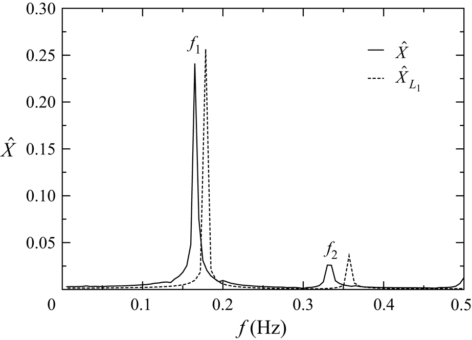
A particle moving on a limit cycle makes a periodic motion in which the components of the trajectory  $\boldsymbol X(t)$ are periodic functions of time. A characteristic quantity of this motion is the period $\tau _1$ that is the inverse of the fundamental frequency $f_1$ of the Fourier spectrum of any of the periodic coordinate functions. The amplitude spectrum $\hat X$ of the $x$ coordinate of the limit cycle is presented in figure 8 (solid line). The fundamental frequency of the limit cycle is $f_1=0.165$ Hz, corresponding to the non-dimensional frequency $F_1=13.33$. The spectrum of the limit cycle compares very well with the spectrum of the fluid motion on the closed streamline that is shown by a dashed line for comparison. To determine the asymptotic decay to the limit cycle, the distance functions $d_n$ from the fixed point in the Poincaré plane for all forty realisations are fitted by (5.3). The result is shown in figure 9(b), yielding the decay rate $\sigma =0.743$.
Amplitude spectrum  $\hat X(f)$ (solid line) of the trajectory of a particle with $a=0.0272$ ( $a_{p}=1.1$ mm) and $\varrho =1.0001$ moving on its periodic attractor with fundamental frequency $f_1=0.165$ Hz ( $F_1=13.33$) in comparison with the spectrum $\hat X_{L_1}$ of the numerically determined closed streamline (dashed line).
(a) Poincaré section on  $y=0$ of a trajectory of a single particle (black dots and lines) with $a=0.0272$ and $\varrho =1.0001$. The final phase from $\tau = 6.4335$ onwards is shown by red dots. Grey dots indicate the largest contiguous KAM torus; the white diamond marks the closed streamline; and the circle defines the threshold distance $d^*$ for Poincaré points to be included in the fit (5.3). (b) The distance function $d_n$ for 40 realisations (grey plus signs). A fit (solid black line) of the data according to (5.3) yields the attraction rate $\bar \sigma =0.766\pm 0.07$.
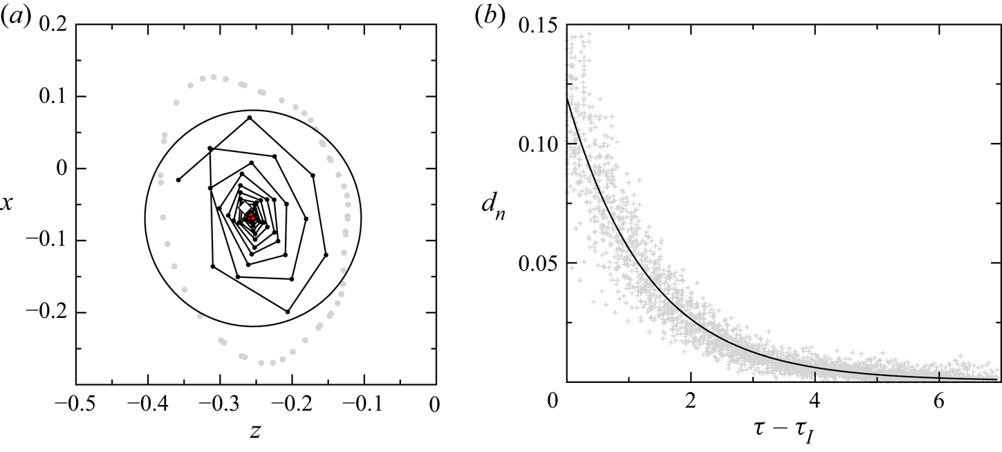
In addition, figure 9(a) shows the Poincaré section of a representative trajectory (black and red dots) in relation to the largest of the inner contiguous KAM tori (grey dots), the closed streamline (diamond) and the threshold condition (circle with radius  $d^*$ about $(x^*,z^*)$).
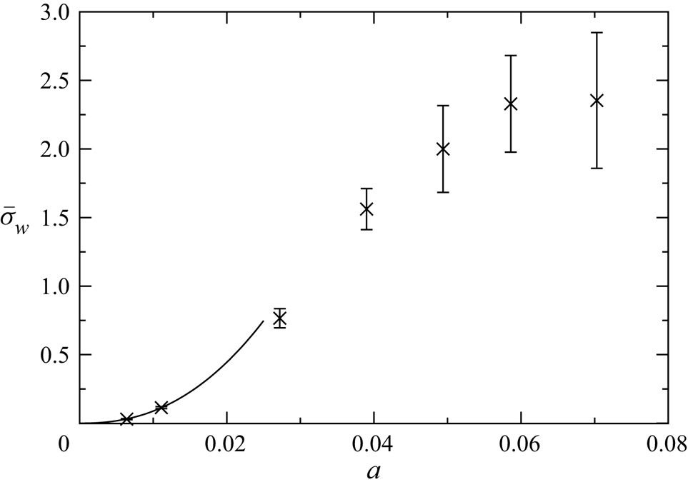
Figure 10 shows the mean attraction rate  $\bar \sigma := N^{-1}\sum _{n=1}^N \sigma _n$, where $\sigma _n$ is determined according to (5.3), $n$ numbers the samples, and $N$ is the number of repeated experiments for each particle. Data ( $\times$) are collected for all particles with $\varrho =1.0001$. As can be seen, the rate of attraction to the limit cycle increases with the particle size $a$. As will be shown below, the density difference between the particles and the fluid is too small to relate the attraction to inertial effects. Therefore, the attraction rates found are attributed mainly to the wall effect, i.e. the confinement effect of a finite size particle, and will be denoted $\bar \sigma _w$ henceforth. Also included in the graph is a power-law fit (solid line) to the three points given by the origin $(0,0)$ and the data for the two smallest particles. We find the approximation $\bar \sigma _w = ca^b$ with $c=3968$ and $b=2.32$ valid for $a < 0.012$. Other fit functions, e.g. polynomials, have been tested as well. They all lead to similar implications regarding the contribution of the wall effect to the attraction rate of heavier particles with size up to $a=0.0120$ (figure 15 below).
Mean attraction rates  $\bar \sigma _w$ to the period-one attractors for nearly neutrally buoyant particles with radii $a=0.0064$, $0.0111$, $0.0272$, $0.0390$, $0.0494$, $0.0586$, $0.0704$, corresponding to $a_{p} = 0.26$, 0.45, 1.10, 1.58, 2.00, 2.37, 2.85 mm. The solid line is a fit $\bar \sigma _w = ca^b$ ( $c=3968$, $b=2.32$) to the data for the smallest particle sizes (see text).
6.1.2. Limit cycle of period six
For the smallest particle size  $a=0.0064$ and for $\varrho =1.0001$, we find, in addition to the limit cycle of period one near $L_1$, another limit cycle of period six. The limit cycle to which the particle is attracted depends on the initial conditions. The period-six limit cycle is found near the closed streamline $L_6$. Figure 11 shows a three-dimensional view of trajectories on the two attractors (blue) and Poincaré sections on $y=0$ during the time interval $t\in [6700,7200]$ s. At this time, particle trajectories have converged to the period-six attractor up the size of the blue dots shown in figure 11(b). The period-six KAM tori seem to be a robust feature of the flow, because they also exist in the exactly cubical cavity at the same Reynolds number (Romanò et al. Reference Romanò, Türkbay and Kuhlmann2020).
Sixteen trajectories for  $a=0.0064$ ( $a_{p}=0.26$ mm) and $\varrho =1.0001$ recorded during $t\in [6700,7200]$ s. (a) Three-dimensional view of the period-six attractors (blue) and transient toroidal trajectories that are ultimately attracted to one of the two period-one limit cycles. (b) Poincaré sections on the plane $y=0$ (black, blue) of the particle trajectories shown in (a). Poincaré sections of numerically computed streamlines are shown as light grey dots.
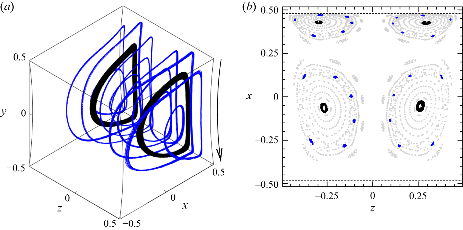
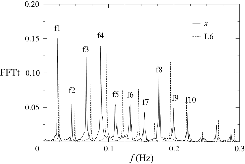
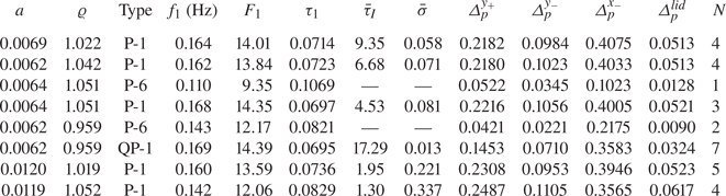
Also shown in figure 11 is a three-dimensional view of trajectories and a Poincaré section of particles that end up on one of the two period-one limit cycles near  $L_1$. The attraction is so weak that these particles have not yet reached their periodic orbit at $t=7200$ s (see figure 19b). In comparison, the attraction to the period-six orbit is one order of magnitude faster (table 3). This can be explained by the close proximity to the moving wall of the closed streamline $L_6$ and the period-six limit cycle, which are shown in maroon and light grey, respectively, in figure 6(b). Therefore, a particle near $L_6$ repeatedly experiences a much stronger wall-induced repulsive force than the same particle (dark grey in figure 6b) when it moves near $L_1$. From the spectrum of the period-six attractor shown in figure 12, we find the fundamental frequency $f_1=0.133$ Hz. The subharmonics at $f_1/6$ of order six and its integer multiples clearly indicate the period-six motion on this attractor. Properties of the limit cycles for all nearly neutrally buoyant particles found are collected in table 3. The correlation between the limit cycles for the particles and numerically computed closed streamlines can be seen by comparing tables 3 and 2.
Amplitude spectrum  $\hat X$ of a trajectory on the period-six attractor with $f_1=0.133$ Hz ( $F_1=10.91$) for $a=0.0064$ ( $a_{p}=0.26$ mm), $\varrho =1.0001$, ${\textit {Re}}=100$ and $T=24.3\,^\circ$C. For comparison, the spectrum $\hat X_{L_6}$ of the numerically determined closed streamline is shown as a dashed line.
Properties of measured trajectories of nearly neutrally buoyant particles on their periodic attractors for  ${\textit {Re}}=100$ and $\varrho =1.0001$. Specified are the type (period), fundamental frequencies $f_1$ (dimensional) and $F_1$ (dimensionless), turnover time $\tau _1 = F_1^{-1}$, initial transient time $\bar \tau _I$ required to approach the attractor up to the distance $d_n \le 0.15$ (in the plane $y=0$), asymptotic attraction rate $\bar \sigma _w$, the closest wall-normal distances from the boundaries $\varDelta _{p}$ (the boundary is indicated by the superscript), and the number of samples $N$ used for averages.
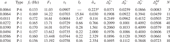 $^a$The attraction rate for the P-6 attractor was evaluated by fitting exponentially the local minima of the $X(\tau )$ coordinate of the trajectory.
Even though period-seven KAM tori exist in the flow, embedded in the period-one KAM system, we have not found a period-seven attractor. This may be related to not having probed a particle size suitable for attraction. Since  $L_7$ approaches the moving wall even closer than $L_6$ (table 2), the particles that could be attracted to a limit cycle of period seven are expected to be even smaller than $a=0.0064$. A further difficulty of finding such attractors may arise from the particle size selectivity, which is related to the small diameter of the period-seven KAM structures.
6.2. Forces along the trajectories of density-matched particles
In order to assess major forces acting on the particle during its motion, we used a measured particle trajectory and computed all flow gradients along this trajectory from the unperturbed flow field obtained numerically. The flow velocity at the position of the particle is determined by polynomial interpolation of the numerical velocity field, while the velocity of the particle is calculated by central differences of the measured discrete position data. For small particles, the forces arising in the Maxey–Riley equation (Maxey & Riley Reference Maxey and Riley1983) are of interest.
Results for a particle with  $a=0.0111$ and $\varrho =1.0001$ for ${\textit {Re}}=100$ are shown in figure 13(a) during the initial (transient) phase, and in figure 13(b) during the motion on the limit cycle. Figures 13(a i) and 13(b i) show the particle location in the form of $x(\tau )$ (black), $y(\tau )$ (red) and $z(\tau )$ (green). Figures 13(a ii–iv) and 13(b ii–iv) show the $x$,
$x$,  $y$ and $z$ components of the acceleration terms evaluated. For the $x$ component, figures 13(a ii) and 13(b ii) show the pressure force, including the added mass effect $(3/2)R\,\mathrm {D} u/\mathrm {D} \tau$ (black), Faxén's correction to the added mass $(a^2/20)\,\mathrm {D} ({\nabla }^2 u)/\mathrm {D} \tau$ (red), the Stokes drag $-R\,{\textit {St}}^{-1}\,(\dot X - u)$ (green) and Faxén's correction to the Stokes drag $(a^2/6)R\,{\textit {St}}^{-1} {\nabla }^2 u$ (blue). Here, $R=2/(1+2\varrho )$. The lines in the plots for the $y$ and $z$ components have the corresponding meanings.
Trajectory  $(x,y,z)$ (plot (i)) of the particle with $a=0.0111$ and $\varrho =1.0001$ for ${\textit {Re}}=100$. Plots (ii)–(iv) show different components of the acceleration in the $x$,
$x$,  $y$ and $z$ directions, respectively. For an explanation of the colour code, see the text. (a) Initial transient phase. (b) Final phase when the particle moves on its attractor.
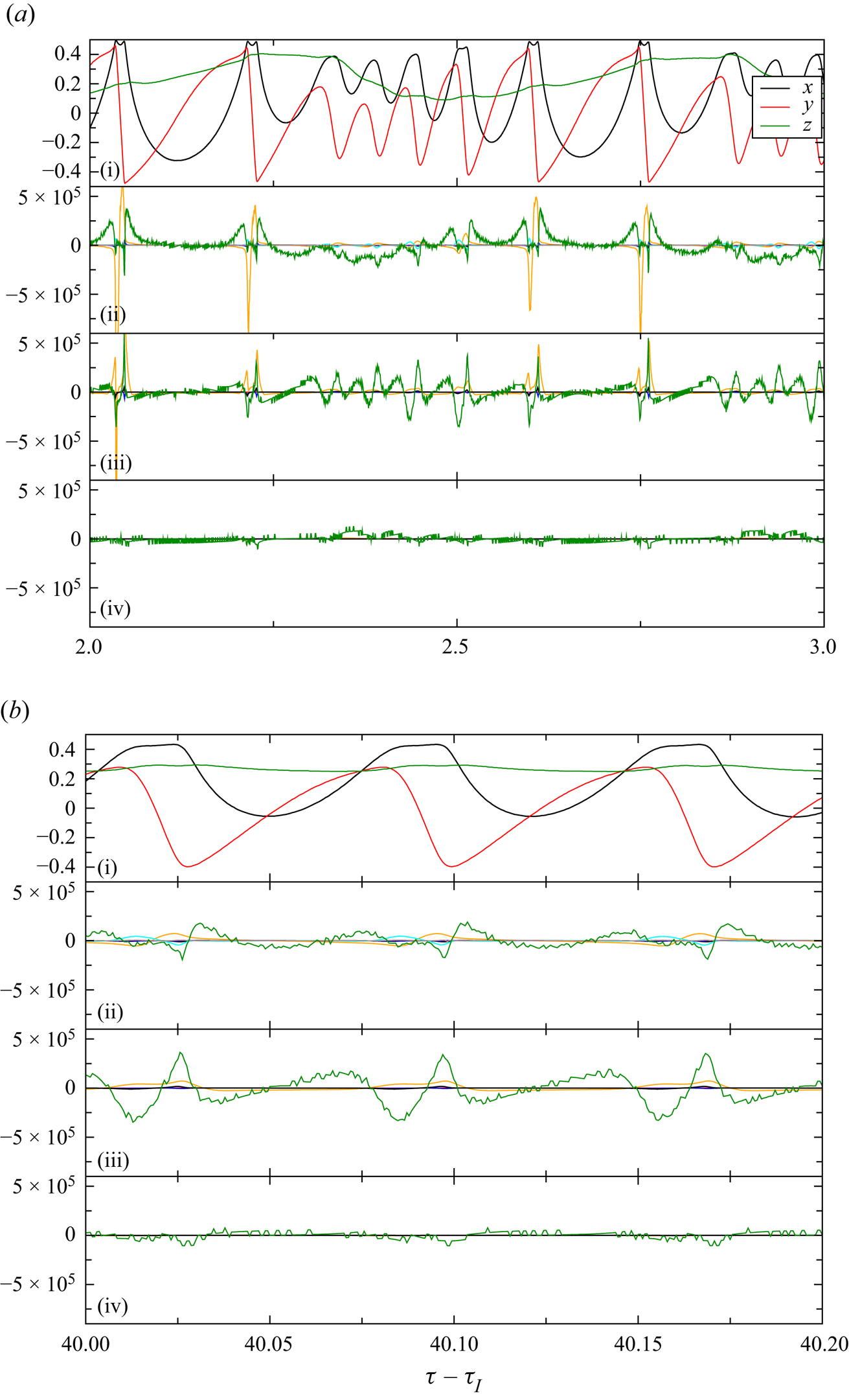
In addition to the above terms, we show forces which are not contained in the Maxey–Riley equation. They derive from the particle velocity, the unperturbed velocity gradient and the distances to the walls. These forces were computed to estimate the magnitude of the corresponding effect on the particle motion. The additional drag force on a particle viscously settling according to Brenner's correction to the drag coefficient  $\lambda$ has been computed as $-R\,{\textit {St}}^{-1}\sum _{i=1}^3(\lambda _i -1) \dot {\boldsymbol X}_{i,\perp }$, where the sum runs over the contributions from the top wall ( $i=1$), the curved moving wall ( $i=2$) and the bottom wall ( $i=3$), $\lambda _i$ is the drag coefficient evaluated corresponding to the distance from the $i$th wall, and $\dot {\boldsymbol X}_{i,\perp }$ is the particle velocity normal to the $i$th wall. The resulting contributions, decomposed into Cartesian components, are shown in orange in figure 13. To estimate a possible migration effect, we also monitor (in the $x$ plot only) Saffman's lift force in the $x$ direction $0.727\varrho ^{-1}\,{\textit {St}}^{-1/2}\,(v-\dot Y)\,|\partial v /\partial x|^{1/2}{\rm sgn}(\partial v /\partial x)$ (cyan; Saffman Reference Saffman1965, Reference Saffman1968). Finally, we also consider the lift force (in the $x$ plot only) for a freely rotating particle near a plane wall according to the formula given by Cherukat & Mclaughlin (Reference Cherukat and Mclaughlin1994) (brown).
Throughout its motion, the largest forces on the particle arise during the closest approach to the moving wall. Of these forces, viscous forces (green, orange) dominate. We first consider the motion on the attractor. From figure 13(b iii), one can see that the passage of the particle near the moving wall experiences a viscous drag (green) that is directed in the negative  $y$ direction due to the flow acceleration caused by the wall motion and the particle being slightly heavier than the fluid. In the $x$ direction, viscous forces dominate as well. It is seen that the particle starts lagging behind the flow even upon approaching the moving wall. The positive drag forces indicate that the particle is kept away from the moving wall. This is an important property of the lump wall effect (see also the model of Hofmann & Kuhlmann Reference Hofmann and Kuhlmann2011). The repulsion effect is also signalled by the positive contribution of the correction to the viscous drag according to Brenner's drag coefficient $\lambda$ (orange). On the other hand, Saffman's lift force (cyan) tends to push the particle towards the wall. Since the Saffman lift may not be correct near a moving wall, we also included the lift force according to the formula of Cherukat & Mclaughlin (Reference Cherukat and Mclaughlin1994) for a freely rotating particle (brown). The lift force of Cherukat & Mclaughlin (Reference Cherukat and Mclaughlin1994) is much smaller than Saffman's formula suggests, and particle lift seems to be insignificant overall.
The initial transient phase is shown in figure 13(a). This phase is very important for the attraction rate of the particle attraction to the limit cycle (see e.g. figure 9 for  $a=0.0272$). One can see that the forces experienced by the particle upon the interaction with the moving wall are even stronger and more impulsive than during its motion on the attractor (figure 13b). The reason is that during the initial phase, the particle approaches the wall even closer and in more irregular intervals. Therefore, the overall dynamics is clearly dominated by the particle–wall interaction.
Finally, we consider the largest density-matched particle with  $a=0.0704$ and $\varrho =1.0001$ for ${\textit {Re}}=100$. The forces acting during the motion on the attractor are displayed in figure 14. For this large particle, the wall interaction is even more dominant. Again, viscous forces (green, orange) are dominant and signal the wall repulsion effect. This is plausible, since the particle approaches the moving wall much closer than its radius (see table 3). For this larger particle, also the pressure force becomes relevant, because of the larger Stokes number. The two negative peaks (black) in the $x$ component tend to keep the particle away from the wall. From these considerations, viscous forces seem to play an important role for the particle dynamics. Since these forces arise predominantly during the passage of the particle past the moving wall, its attraction to the limit cycle is attributed to a lump wall effect. Faxén's forces are insignificant, and also lift forces appear to play a very minor role for the particle motion in the present fully three-dimensional flow.
(a) Trajectory  $(x,y,z)$ of the particle with $a=0.0704$ and $\varrho =1.0001$ for ${\textit {Re}}=100$ moving on its attractor. (b–d) Different components of the acceleration in the $x$,
$x$,  $y$ and $z$ directions, respectively. For an explanation of the colour code, see the text.
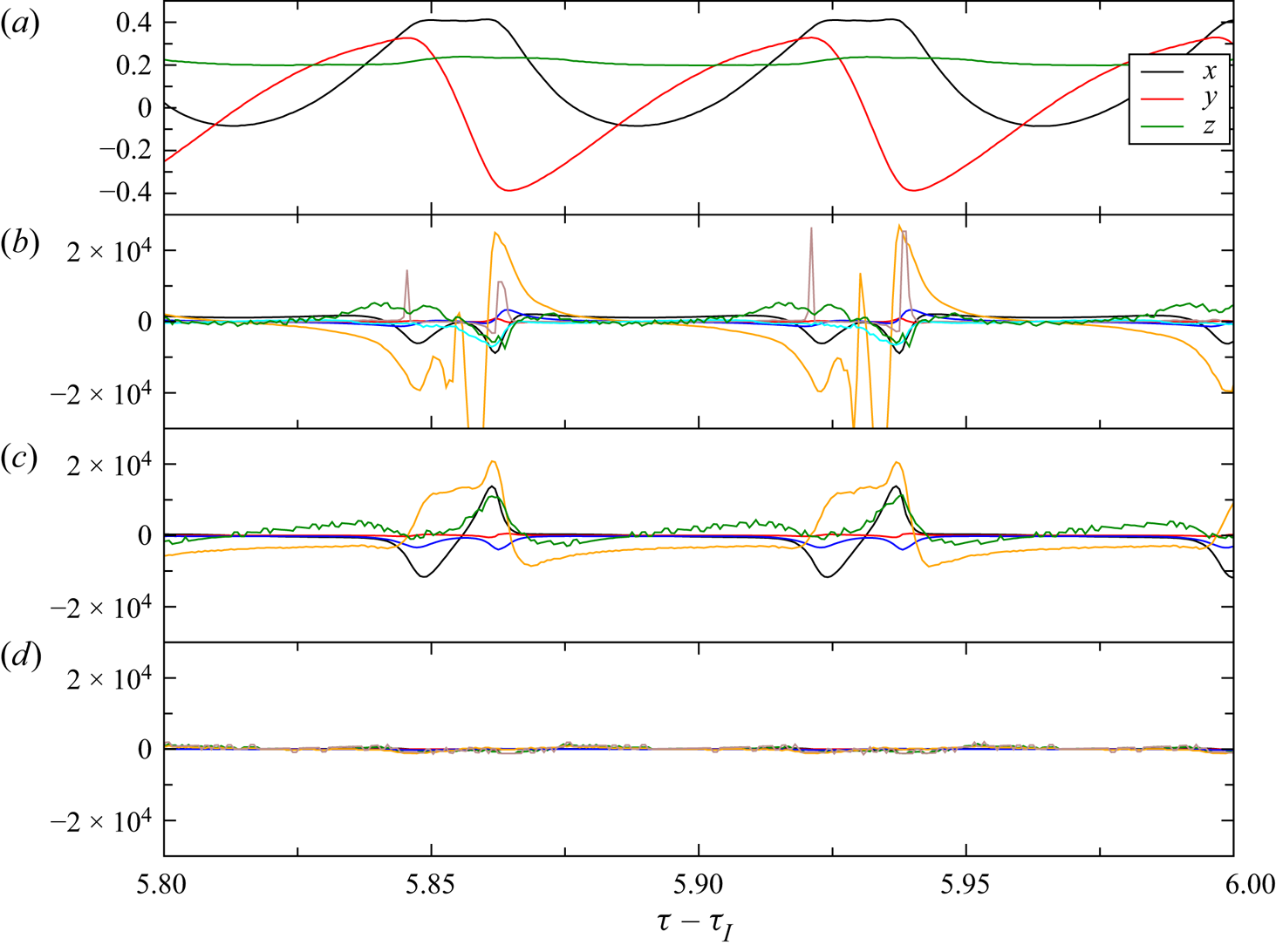
From the Stokes drag force shown in figures 13(b) and 14, the slip velocity along the limit cycle seems to remain considerable even between the particles’ visits of the moving wall. The  $y$ component $\dot Y-v$ of the slip velocity computed varies almost linearly from 5 % to $-7\,\%$ of the wall velocity during the particle's motion in the bulk (from the departure from to the arrival at the moving wall). We cannot rule out completely that a certain amount of slip is caused by extra drag forces on the particle provoked by the confinement of the system by the stationary and moving walls. However, the computed slip velocity in the bulk was found to be almost identical for the particles with $a=0.0704$, 0.0111 and 0.0064 (not shown). This indicates that the computed data overestimate the slip due to different sources of error. The most obvious source of error, which alone can account for the above residual slip, is the accuracy of $|\Delta \boldsymbol X| = 0.0074$ ( $\pm 0.3$ mm) by which the position of the particle can be measured. Other errors arise from the sampling time of $\Delta t\approx 6.1\times 10^{-4}$ (0.05 s) due to which the direction of the particle velocity computed from secants of the trajectory deviates from the true particle velocity in regions of fast motion on curved trajectories. Other sources of error are the limited resolutions of the camera sensors. To illustrate this point, the Stokes drag is the only quantity that is shown unfiltered in figures 13 and 14, and thus appears noisy. Finally, the flow in the experiment can deviate from the numerically computed flow such that also the measured particle velocity $\dot {\boldsymbol X}$ can deviate from the numerical flow velocity at the position but in the absence of the particle. An elimination of these errors and a clarification of the magnitude and character of the true residual drag forces acting in the bulk are very difficult due to the nature of the problem.
6.3. Motion of inertial particles
For particles heavier than the fluid with density difference up to 5 %, a picture emerges that is similar to that for density-matched particles. For all particle sizes investigated, there always exists a period-one attractor near the closed streamline  $L_1$. The properties of the attractors are provided in table 4. Among the cases considered, the limit cycle with the largest displacement from $L_1$ in the Poincaré plane arises for $a = 0.0119$ ( $a_p = 0.48$ mm) and $\varrho = 1.052$. The Poincaré section of the attractor is shown by black symbols in figure 5. From the Poincaré section, the location of the periodic orbit relative to the closed streamline does not follow the systematic trend exhibited by the neutrally buoyant particles. In the Poincaré plane shown, the inertial particle (black) is displaced from the closed streamline much further and in a different direction as compared to a neutrally buoyant particle of comparable size (blue).
Properties of measured trajectories of inertial particles on their attractors for  ${\textit {Re}}=100$. Specified are the type of attractor (P means periodic, QP means quasi-periodic), fundamental frequencies $f_1$(dimensional) and $F_1$(dimensionless), turnover time $\tau _1=F_1^{-1}$, initial transient time $\bar \tau _I$ required to approach the attractor up to the distance $d_n \le 0.15$ (in the plane $y=0$), asymptotic attraction rate $\bar \sigma$, the closest wall-normal distances from the boundaries $\varDelta _{p}$ (the boundary is indicated by the superscript), and the number of samples $N$ used for averages.
From (4.1), the attraction/repulsion rate for weakly inertial-buoyant particles is expected to scale  $\sim (\varrho -1)\,{\textit {St}}$ (see also Muldoon & Kuhlmann Reference Muldoon and Kuhlmann2016; Wu et al. Reference Wu, Romanó and Kuhlmann2021). However, the attraction rates measured and shown as red dots in figure 15 do not exhibit the expected overall linear dependence. It is striking, however, that the attraction rates for small particles of nearly the same size with $a\in [0.0062, 0.0064, 0.0069]$ as well as the attraction rate for the neutrally buoyant particle with $\varrho =1.0001$ (blue square) exhibit a linear dependence on $(\varrho -1)\,{\textit {St}}$, merely offset from the linear law (shown as a solid line) that passes through zero. Furthermore, the slope of the line connecting the growth rates of the two larger particles of similar size ( $a\in [0.0119, 0.0120]$) is almost the same as for the smaller particles. These observations, in particular the offset of the growth rate for the nearly neutrally buoyant particle (blue square), suggest that the attraction rate $\bar \sigma =\bar \sigma _w +\bar \sigma _i$ comprises a superposition of a size effect ( $\bar \sigma _w$, due to the wall repulsion) and an inertial effect ( $\bar \sigma _i$). A linear superposition is a valid assumption here, because the forces responsible for the attraction are small, which is confirmed by the small particle Reynolds number (table 1), leading to a small attraction rate, which justifies a linearisation of the dynamics. We note that the particle Reynolds number ${\textit {Re}}_p$ and corresponding Stokes drag are possibly smaller, because of the difference due to numerical error and imperfections between the numerically computed velocity at the location of the particle and the unperturbed experimental velocity, respectively, which could not have been measured.
Measured total mean attraction rate  $\bar \sigma$ (blue square, red dots) to the period-one limit cycle for ${\textit {Re}}=100$ as function of $(\varrho -1)\,{\textit {St}}$ for six particles with different sizes and densities as indicated. The radii are (from left to right) $a\in [0.0064, 0.0069, 0.0062, 0.0064, 0.0120, 0.0119]$ with corresponding densities $\varrho \in [1.0001, 1.022, 1.042, 1.051, 1.019, 1.052]$. The inertial part $\bar \sigma _i$ of the attraction rate is shown by black crosses. The solid line is a linear regression of $\bar \sigma _i$ (see text).

To test the superposition principle, we compute the inertial attraction rate  $\bar \sigma _i$ by subtracting from the measured total attraction rate $\bar \sigma$ the wall-induced attraction rate $\bar \sigma _w$ found for nearly neutrally buoyant particles. Since the particle sizes in figure 15 range up to $a\approx 0.012$, we use the power-law fit to the three smallest data points (including $(\bar \sigma _w,a)=(0,0)$), which is shown by the solid line in figure 10. As a result, we obtain the inertial attraction rate $\bar \sigma _i$ to the period-one limit cycle, which is shown by crosses in figure 15. As can be seen, the data for $\bar \sigma _i$ are consistent with the expected linear dependence. A linear regression (solid line) yields $\bar \sigma _i = c(\varrho -1)\,{\textit {St}}$ with $c=1.24\times 10^5$. Based on this correlation, the inertial attraction rate for the largest density-matched particle from figure 10 with $a=0.0704$ is $\bar \sigma _i=1.39\times 10^{-2}$. This is only $0.6$ % of the attraction rate $\bar \sigma _w=2.354$ measured. This indeed shows that the attraction to the limit cycle is almost entirely due to the wall effect for the particles with $\varrho =1.0001$ (figure 10).
In a similar way as for nearly neutrally buoyant particles, we also find period-six attractors for heavier and lighter particles than the fluid. An example for a heavy particle is shown in figure 16 for  $a=0.0064$ and $\varrho =1.051$. In three out of four realisations, the heavy particle is attracted to one of the period-one limit cycles (black), whereas one realisation shows attraction to a period-six attractor (blue) in the vicinity of one of the period-six KAM tori. The attraction rate to the period-six limit cycle is difficult to determine due to the very short asymptotic phase (the KAM tori are small) such that the time required for the attraction depends sensitively on the initial conditions, i.e. on the initial chaotic motion.
Four trajectories for  $a=0.0064$ ( $a_{p}=0.26$ mm) and $\varrho =1.051$ recorded during $t\in [5500,6000]$ s. (a) Three-dimensional view of the period-one (black) and period-six (blue) attractors for the particle. (b) Poincaré sections on the plane $y=0$ (black, blue) of the particle trajectories shown in (a). Poincaré sections of numerically computed streamlines on the reconstructible KAM tori are shown as light grey dots.
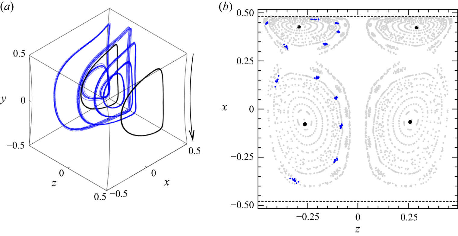
The attractors for a light particle with  $a=0.0062$ and $\varrho =0.959$ are shown in figure 17. We find attractors near $L_1$ (black) and $L_6$ (blue). Now, however, the attractors are not periodic, but quasi-periodic. The reason is the change of the sign of $\varrho -1$ which renders a pure inertial-buoyant limit cycle emerging from the closed streamlines to change its stability. Therefore, unstable limit cycles of period one and six must exist for $\varrho -1 < 0$ if the motion would be purely inertial-buoyant. Obviously, such unstable limit cycles also exits under the present (additional) wall effect. Therefore, the particle–wall interaction cannot prevent the unstable limit cycles. However, the repulsion of the particles from the moving wall stabilises the particle motion on a quasi-periodic orbit in some distance from the respective unstable limit cycle.
Nine trajectories for  $a=0.0062$ ( $a_{p}=0.25$ mm) and $\varrho =0.959$ recorded during $t\in [12000,14000]$ s. The corresponding non-dimensional time interval is $[140.5 ,163.9]$. (a) Three-dimensional view of the toroidal period-one (black) and period-six (blue) attractors. (b) Poincaré sections on the plane $y=0$ (black, blue) of the particle trajectories shown in (a). Poincaré sections of numerically computed streamlines on the KAM tori are shown as light grey dots.
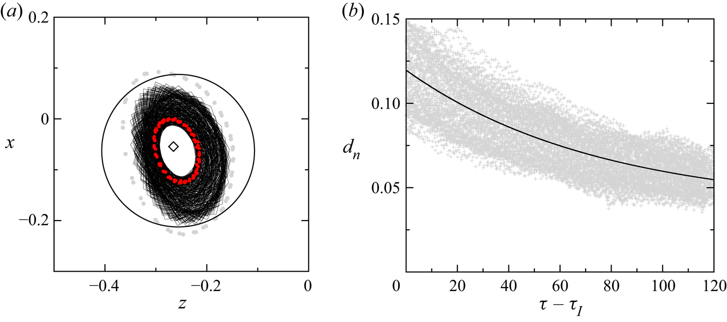
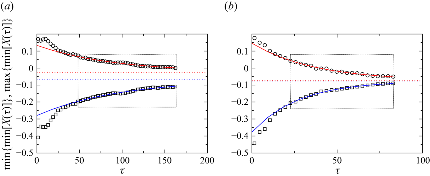
The attraction dynamics of the same light single particle ( $a=0.0062$, $\varrho =0.959$) to the period-one torus is shown in figure 18(a). The mean attraction rate is $\bar \sigma =0.0131$, much smaller than values for all other inertial particles with $\varrho >1$. This can be explained by the quasi-periodic attractor being caused by a balance of opposing weak forces (inertia and wall repulsion). The attraction rate has been computed as described in § 5 using data from seven realisations (figure 18b). To check this result, the evolution of the minima of $X(\tau )$ for a single representative trajectory was considered. For a quasi-periodic orbit, the minima of $X(\tau )$ will vary within a certain range and would not converge. To monitor the range of variation, the maximum and minimum over all minima of $X(\tau )$ satisfying $X < 0.2$ were considered. Within temporal bins of 5000 data points corresponding to $\Delta \tau _{bin}=2.926$, the maximum (upper envelope) and the minimum (lower envelope) of all minima of $X(\tau )$ were obtained. Figure 19(a) shows the evolution of the maximum (circles) and the minimum (squares) of the minima of $X(\tau )$. Fitting the last two-thirds (dotted rectangle) of the envelopes to exponentials (solid red and blue lines), we find slightly different attraction rates $\sigma _{max(min)}=0.0111$ (red) and $\sigma _{min(min)}= 0.0105$ (blue). Both values are within the error bar by which $\bar \sigma$ was determined from the ensemble average (figure 18b). Since the two envelopes extrapolate to different values for $\tau \to \infty$ (horizontal dotted lines), the asymptotic state is indeed quasi-periodic. Near its minimum $x$ coordinate, the attracting torus has diameter in the $x$ direction $D_x = 0.0439$. The slight scatter of the black Poincaré points (instead of a sharp torus) in figure 17(b) can be explained by the particle not yet having reached its asymptotic attractor, which is confirmed by figure 19(a). For comparison, figure 19(b) shows the same analysis for the smallest particle ( $a=0.0064$, $\varrho =1.0001$), which is nearly density matched. It can be seen that the data extrapolate to a limit cycle.
(a) Poincaré section on  $y=0$ of the trajectory of a single particle (black lines) with $a=0.0062$ and $\varrho =0.959$. The Poincaré points during the last phase $\tau \in [156.9, 163.8]$ are shown as red dots (the total measurement time was 3.9 h). Grey dots indicate the largest numerically reconstructible contiguous KAM torus, and the diamond marks the closed streamline. (b) The distance function $d_n$ for seven realisations ( $+$). A fit of the data according to (5.3) (solid black line) yields the attraction rate $\bar \sigma =0.0133\pm 0.0043$.
Maxima (circles) and minima (squares) of the relative minima of the  $x$ coordinate of a single trajectory for ${\textit {Re}}=100$. Each symbol circle (square) is the maximum (minimum) value of the relative minima of $X(\tau )$ within a temporal bin of width $\Delta \tau _{bin}=2.926$. The red and blue solid curves are exponential fits to the binned maxima and minima, respectively. The dotted horizontal lines indicate asymptotic values for $\tau \to \infty$. (a) Plot of 56 bins for an inertial particle with $a=0.0062$ ( $a_{p}=0.25$ mm) and $\varrho =0.959$, yielding $\max \{\min [X(\tau )]\} = -0.0251+0.159\,\mathrm {e}^{-0.0116 \tau }$ (red curve) and $\min \{\min [X(\tau )]\} = -0.0690-0.211\,\mathrm {e}^{-0.0105 \tau }$ (blue curve). (b) Plot of 28 bins for a neutrally buoyant particle with $a=0.0064$ ( $a_{p}=0.26$ mm) and $\varrho =1.0001$, yielding $\max \{\min [X(\tau )]\} = -0.0740 + 0.220\,\mathrm {e}^{-0.0277 \tau }$ (red curve) and $\min \{\min [X(\tau )]\} = -0.0765 - 0.301\,\mathrm {e}^{-0.0368 \tau }$ (blue curve).
7. Results for ${\textit {Re}}=200$

7.1. Motion of nearly neutrally buoyant particles
The behaviour of nearly neutrally buoyant particles in the flow with  ${\textit {Re}}=200$ is similar to that for ${\textit {Re}}=100$. However, the shape and multitude of the periodic attractors differ due to the more intricate structure of the KAM tori for ${\textit {Re}}=200$. Furthermore, the attraction rates are larger than for ${\textit {Re}}=100$ due to the higher flow velocities and the closer proximity of the KAM structures to the moving wall, from which a stronger wall effect results.
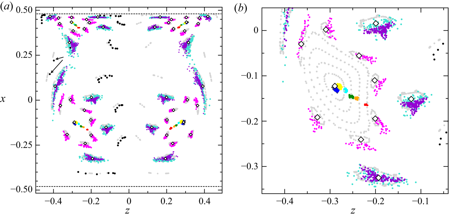
Figure 20(a) shows an overview on the attracting sets in the Poincaré plane  $y=0$, with a zoom into the lower left in figure 20(b). For all particle sizes, we find a period-one attractor near $L_1$, best seen in figure 20(b). As $a$ increases, the limit cycles and their mirror-symmetric counterparts near $L_1$ are displaced in the negative $x$ direction, away from the moving wall and towards the symmetry plane $z=0$, similarly as for ${\textit {Re}}=100$. Moreover, as $a$ increases, the projections of all the period-one limit cycles onto the $(x,y)$ plane (figure 21) are pushed away from the moving wall due to the hindered particle motion caused by its size, and extend further into the positive $y$ direction. This trend was observed also for ${\textit {Re}}=100$, albeit not as clearly.
(a) Poincaré sections on  $y=0$ of trajectories of nearly neutrally buoyant spherical particles ( $\varrho =1.0001$) moving on their respective periodic attractor for ${\textit {Re}}=200$. The colour indicates the particle radius: $a = 0.0064$ ( $a_p=0.26$ mm, P-10 black, P-7 magenta, P-4 turquoise, P-1 dark grey), $a=0.0111$ ( $a_p=0.45$ mm, P-4 violet, P-1 blue), $a=0.0272$ ( $a_p=1.10$ mm, P-1 yellow), $a=0.0390$ ( $a_p=1.58$ mm, P-1 cyan), $a=0.0494$ ( $a_p=2.00$ mm, P-1 green), $a=0.0586$ ( $a_p=2.37$ mm, P-1 orange), and $a=0.0704$ ( $a_p=2.85$ mm, P-1 red). For comparison, the Poincaré sections of KAM tori and of closed streamlines are shown as light grey dots. Diamonds indicate closed streamlines. (b) Zoom into the lower left of (a).
(a) Projection onto the  $(x,y)$ plane of trajectories of nearly neutrally buoyant spherical particles ( $\varrho =1.0001$) moving on their limit cycles for ${\textit {Re}}=200$. The arrow indicates the moving wall. (b) Zoom into (a) with the x and y axes scaled differently. The non-dimensional particle radius $a$ and the periodicity of the orbit is given in the legend in (b).

In addition to the period-one limit cycle, we also find limit cycles of periods four (turquoise), seven (magenta) and ten (black) for the smallest particle size with  $a=0.0064$. Note that due to its shape, the period-ten attractor returns only eight times to the Poincaré plane $y=0$. From the total of three full periods visible for the period-ten attractor, the particle returned to the Poincaré plane only during one full period for the ninth return (arrows in figure 20a) and never for the tenth. This effect is caused mainly by the location of the Poinicaré plane (see also figure 21a). Also, particles with the next higher particle size of $a=0.0112$ can be attracted to different limit cycles: in addition to the period-one limit cycle (blue), we find a limit cycle of period four (violet dots).
Characteristic properties of all limit cycles found for  ${\textit {Re}}=200$ are collected in table 5. All limit cycles found form near corresponding KAM tori and associated closed streamlines that are indicated by open diamonds. The limit cycles are created because the corresponding KAM tori approach the moving wall sufficiently closely (see table 5). This property increases the probability for particles to be transferred from the chaotic sea to one of the KAM tori. Once a neutrally buoyant particle is caught in a KAM torus sufficiently close to the moving wall, it is attracted to a limit cycle by the interaction with the moving wall as described by Hofmann & Kuhlmann (Reference Hofmann and Kuhlmann2011).
Properties of measured trajectories on the attractor for nearly neutrally buoyant particles with  $\varrho =1.0001$ as functions of the particle radius $a$ at ${\textit {Re}}=200$. Specified are the type of attractor (P means periodic, QP means quasi-periodic), fundamental frequencies $f_1$(dimensional) and $F_1$ (dimensionless), turnover time $\tau _1=F_1^{-1}$, initial transient time $\bar \tau _I$, asymptotic attraction rate $\bar \sigma _w$, the closest wall-normal distances from the boundaries $\varDelta _{p}$ (the boundary is indicated by the superscript), and the number of samples $N$ used for averages.
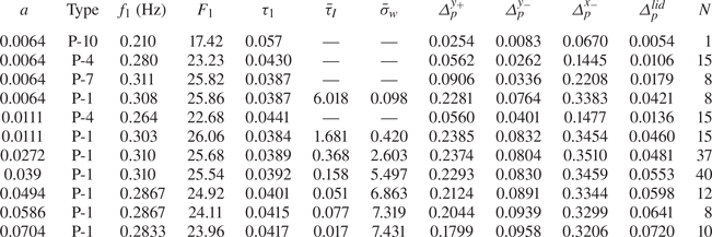
The rates of attraction to the limit cycles have been determined as for  ${\textit {Re}}=100$. Figure 22 presents the mean attraction rate as a function of the particle size $a$. The attraction rates are generally larger than for ${\textit {Re}}=100$, but follow a similar trend with respect to a variation of the particle size. As for ${\textit {Re}}=100$, the mean attraction rate is approximated by a power law $\bar \sigma _w=ca^b$, with $c=5.75\times 10^4$ and $b=2.63$, obtained by fitting to the data for the two smallest particles and the origin.
Mean attraction rate  $\bar \sigma _w$ to the period-one limit cycle as a function of the particle radius for ${\textit {Re}}=200$ and nearly neutrally buoyant particles with $\varrho =1.0001$ and radii $a=0.0064$, $0.0111$, $0.0272$, $0.039$, $0.0494$, $0.0586$, $0.0704$, corresponding to $a_{p} = 0.26$, 0.45, 1.10, 1.58, 2.00, 2.37, 2.85 mm. The solid curve represents a power-law fit $\bar \sigma _w=ca^b$ ( $c=5.75\times 10^4$, $b=2.63$) to the data for small $a$.
$a$.
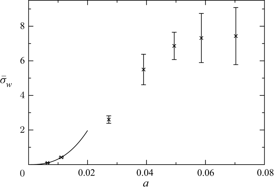
7.2. Motion of inertial particles
As the particle density becomes larger, inertial forces cooperate with the forces from the wall in attracting the particle to a limit cycle. Therefore, the attraction rate increases. For all heavy particles, we find the period-one attractor near  $L_1$, as for ${\textit {Re}}=100$. However, owing to the different fine structure of the KAM template for ${\textit {Re}}=200$, we find other attractors corresponding to the secondary KAM tori. For particles with small inertia, i.e. for $a=0.0069$, $\varrho =1.022$, and $a=0.0120$, $\varrho =1.019$, we find an additional period-twelve limit cycle. An example is shown in blue in figure 23 for $a=0.0069$ and $\varrho =1.022$. The period-twelve attractor forms in the close vicinity of the period-four KAM tori of the flow field. For the heavier particle with $a=0.0130$ and $\varrho =1.061$, the period-twelve attractor is absent. Instead, an attracting period-three limit cycle is found. It cannot be associated directly with a particular KAM structure, but it seems to reflect the shape of the primary KAM tori around $L_1$. The period-three limit cycle is shown in blue in figure 24.
Nine trajectories for  $a=0.0069$ ( $a_{p}=0.28$ mm) and $\varrho =1.022$ recorded during $t\in [3000,3600]$ s. (a) Three-dimensional view of the period-one (black) and period-twelve (blue) attractors. (b) Poincaré sections on the plane $y=0$ (black, blue) of the particle trajectories shown in (a). Poincaré sections of numerically computed streamlines on the corresponding largest reconstructible KAM tori are shown as light grey dots.
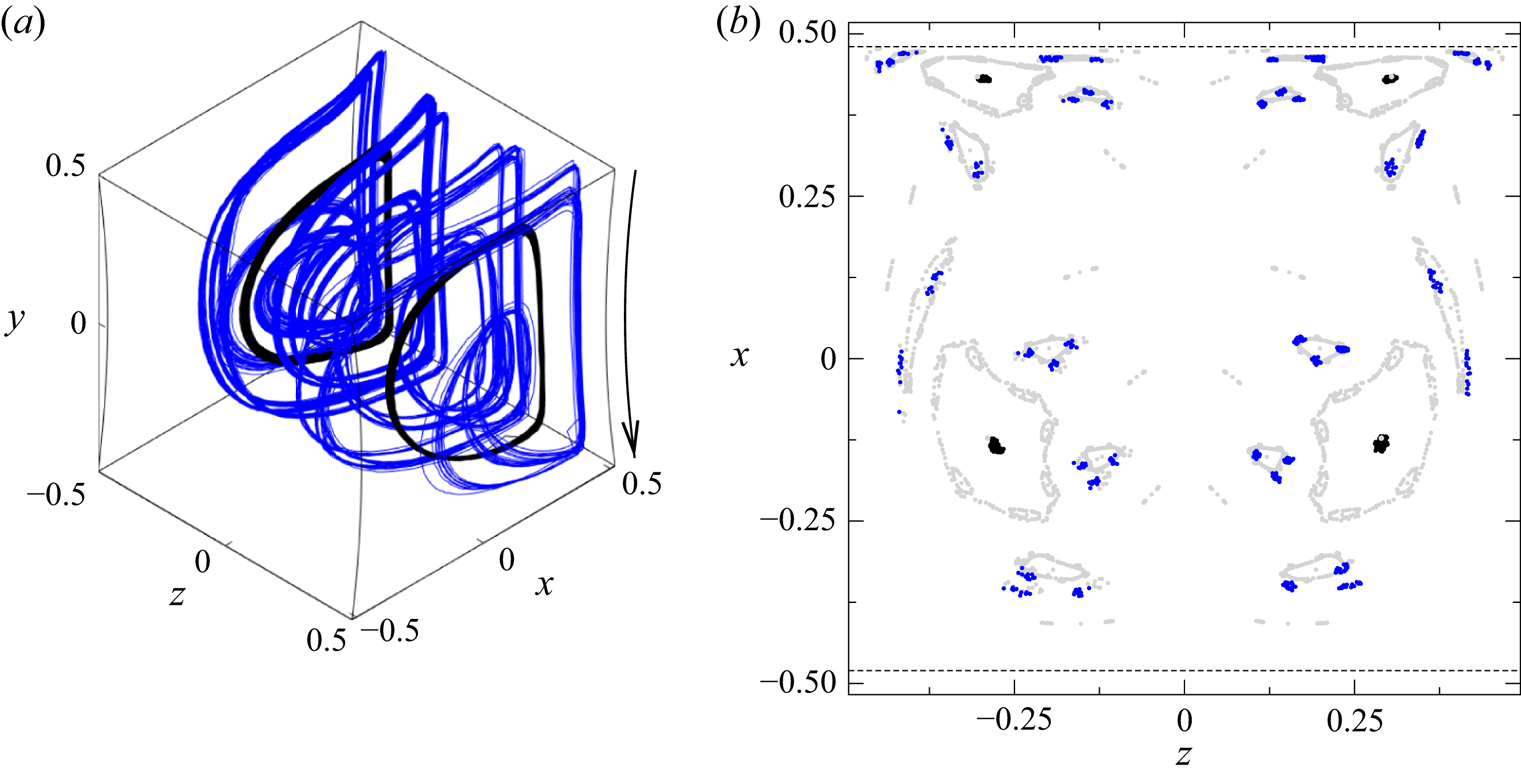
Seventeen trajectories for  $a=0.0130$ ( $a_{p}=0.525$ mm) and $\varrho =1.061$ recorded during $t\in [400,500]$ s. (a) Three-dimensional view of the period-one (black) and period-three (blue) limit cycles. (b) Poincaré sections on the plane $y=0$ (black, blue) of the particle trajectories shown in (a). Poincaré sections of numerically computed streamlines on the corresponding largest reconstructible KAM tori are shown as light grey dots.
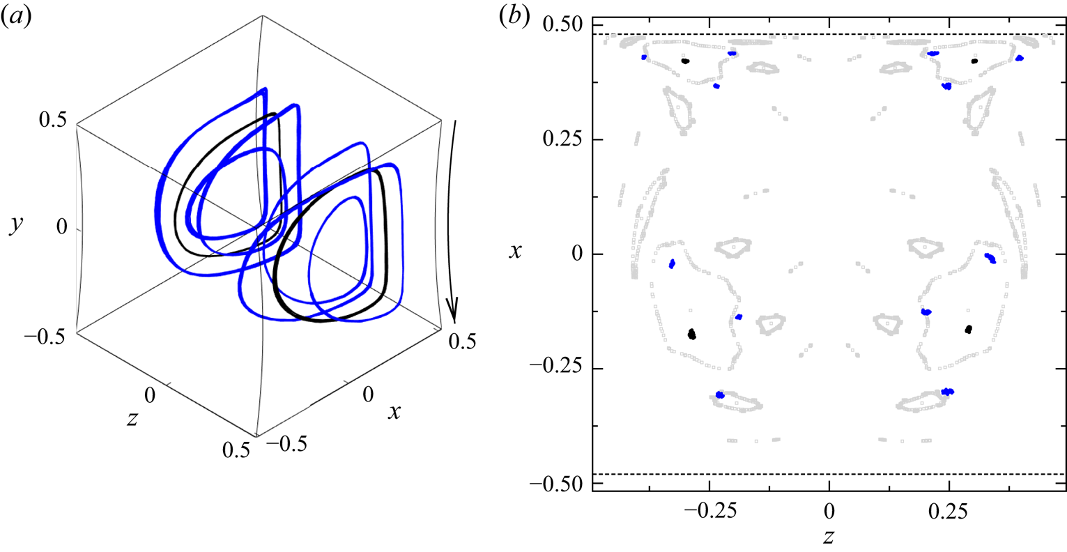
In figure 25, the mean attraction rates for the three heavy particles to their main period-one limit cycle for  ${\textit {Re}}=200$ are shown by red dots as functions of $(\varrho -1){\textit {St}}$. Numerical data are provided in table 6. After subtracting the attraction rate $\sigma _w$ due to the wall effect found for the neutrally buoyant particles (solid line in figure 22), the inertial part $\sigma _i$ of the attraction rate is almost a linear function of $(\varrho -1)\,{\textit {St}}$ (solid line in figure 25).
Mean rates of attraction to the period-one limit cycle for inertial particles with  $\varrho > 1$ as functions of $(\varrho -1)\,{\textit {St}}$. Shown are the total attraction rates $\bar \sigma$ (red dots, blue square) measured and the inertial attraction rate $\sigma _i$ (black crosses) after eliminating the wall effect. Three particles with different radii $a\in [0.0069, 0.0120, 0.0130]$ and corresponding densities $\varrho \in [1.022, 1.019, 1.061]$ were tested. The solid line represents the linear regression $\bar \sigma _i = c (\varrho -1)\,{\textit {St}}$ with $c = 2.23\times 10^5$. The blue square shows $\bar \sigma$ for a particle with $a=0.0064$, $\varrho =0.0001$.
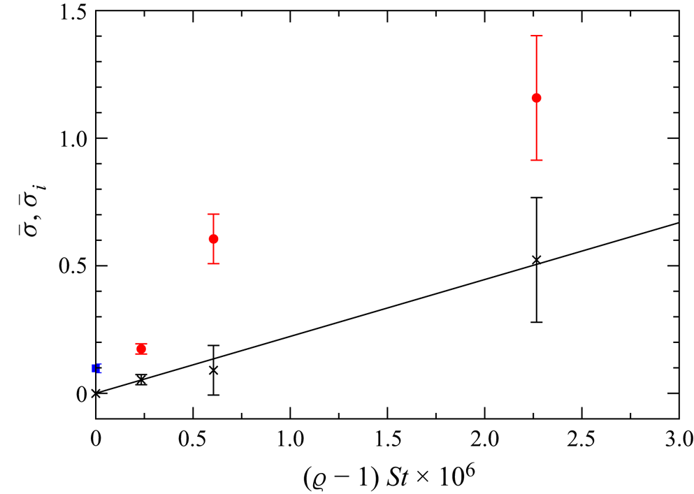
Properties of measured trajectories of inertial particles on their attractors for  ${\textit {Re}}=200$. Specified are the type of attractor (P means periodic, QP means quasi-periodic), fundamental frequencies $f_1$(dimensional) and $F_1$(dimensionless), turnover time $\tau _1=F_1^{-1}$, initial transient time $\bar \tau _I$, asymptotic attraction rate $\bar \sigma$, the closest wall-normal distances from the boundaries $\varDelta _{p}$ (the boundary is indicated by the superscript), and the number of samples $N$ used for averages.
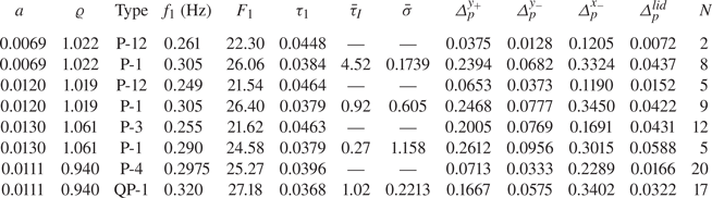
Finally, we investigate the behaviour of a light particle with  $a=0.0112$, $\varrho =0.940$. As expected, the periodic attractor near $L_1$ for heavy particles has become an unstable limit cycle for light particles, which cannot be observed directly. Obviously, the repulsion is strong enough to prevent a wall-induced stable limit cycle that would exist near $L_1$ in the absence of inertia. Only at a certain distance from $L_1$ can the stabilising wall effect balance the destabilising inertia effect leading to a toroidal equilibrium trajectory QP-1 with period one (figure 26a).
Thirty-seven trajectories for  $a=0.0111$ ( $a_{p}=0.45$ mm) and $\varrho =0.940$ recorded during $t\in [1000,1180]$ s. (a) Three-dimensional view of the toroidal period-one attractors QP-1 (black) and the stable period-four limit cycles P-4 (blue). (b) Poincaré sections on the plane $y=0$ (black, blue) of the particle trajectories shown in (a). Poincaré sections of numerically computed streamlines of characteristic KAM tori are shown as light grey dots.
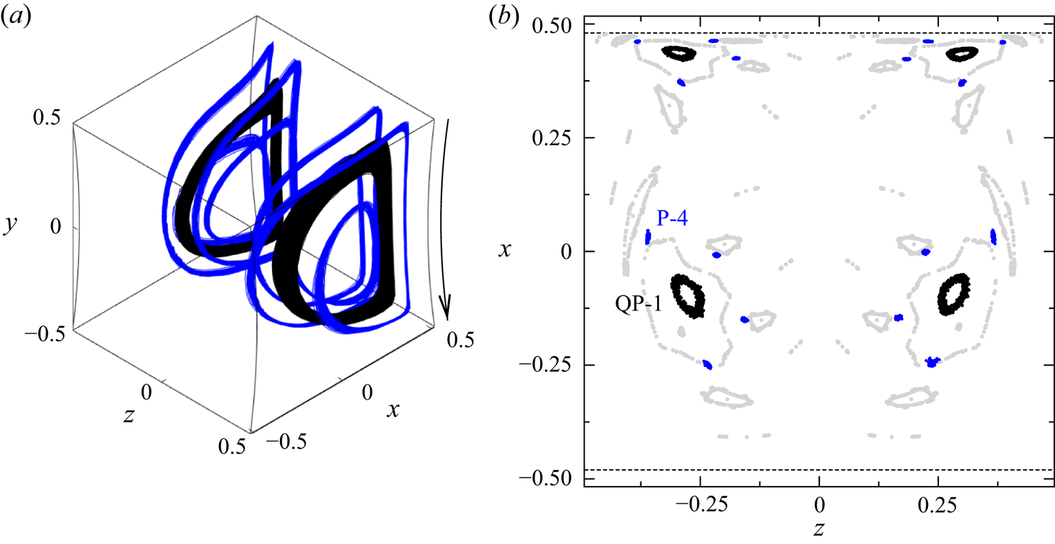
Since inertial forces dominate in the bulk, and repulsive forces from the moving wall decay from the wall within a distance of the order of  $a$, the quasi-periodic attractor should approach the moving wall up to a distance of the order of $a$. In fact, the minimum distance of the quasi-periodic attractor QP-1 from the moving wall is $\approx 3a$ (table 6). The Poincaré section of a particle trajectory on QP-1 is shown by black dots in figure 26(b). In addition, a period-four attractor is found (blue in figure 26), similarly as for the neutrally buoyant particle with a comparable size (violet in figure 20). Even though this attractor is expected to be quasi-periodic, just like the toroidal attractor of period six for ${\textit {Re}}=100$ for the light particle (blue in figure 17), the measured time-asymptotic trajectories cannot be distinguished from a limit cycle. This behaviour might be caused by a dominating wall effect on the particle that overcomes the expected destabilising inertia effect. This interpretation is supported by the much closer approach to the moving wall of the period-four orbit P-4 as compared to the toroidal attractor QP-1 (table 6). The locus of P-4 in the Poincaré plane is somewhat displaced from the closed streamline $L_4$ of period four.
It is interesting to note that the light particle has almost the same attractors as a heavy particle with the same size and the same magnitude of the density mismatch, but with the direction of the wall motion reversed, i.e.  ${\textit {Re}}\to -{\textit {Re}}$. This is demonstrated by the side-by-side comparison in figure 27 of the Poincaré sections for the light particle with $a=0.0111$, $\varrho =0.94$ and ${\textit {Re}}=200$ (on the left) and the ones for the heavy particle with $a=0.0130$ and $\varrho =1.061$ and ${\textit {Re}}=-200$ (reversed wall motion, on the right). This means, in both cases there exists an unstable limit cycle (periodic repeller) surrounded by the observed QP-1 type of attractors (black).
Symmetry of the attractors QP-1 and P-4 with respect to the symmetry  $[{\textit {Re}},(\varrho -1)]\to - [{\textit {Re}},(\varrho -1)]$. Shown are Poincaré sections on the plane $y=0$ of particle trajectories attracted to a period-four limit cycle (blue) and a quasi-periodic orbit (black). For $A$ (to the left of the red line), $a=0.0112$, $\varrho =0.94$ and ${\textit {Re}}=200$. For $B$ (to the right of the red line), $a=0.0130$, $\varrho =1.061$ and ${\textit {Re}}=-200$. Poincaré sections of numerically computed KAM tori are shown as light grey dots.
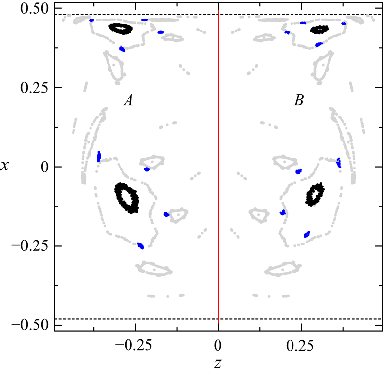
This may appear surprising, because the sign of the density mismatch ( $\varrho -1$) determines the character of the limit cycle, being stable or unstable. To better understand the situation, we consider the inertial equation (4.1) in components:
 $$\begin{align} \dot{X} &= u -(\varrho-1)\, {\textit{St}} [u\,\partial_x u + v\,\partial_y u + w\,\partial_z u ], \end{align}$$
 $$\begin{align}\dot{Y} &= v -(\varrho-1)\, {\textit{St}} [u\,\partial_x v + v\,\partial_y v + w\,\partial_z v + {\textit{Fr}}^{{-}2}], \end{align}$$
 $$\begin{align}\dot{Z} &= w -(\varrho-1)\, {\textit{St}} [u\,\partial_x w + v\,\partial_y w + w\,\partial_z w]. \end{align}$$
The inertial equations (7.1) are invariant under a rotation by  ${\rm \pi}$ about the $x$ axis, corresponding to a reversal of the Reynolds number ( ${\textit {Re}}\to -{\textit {Re}}$)
 \begin{equation} \left(\begin{array}{@{}c@{}}
u \\ v \\ w \end{array}\right) (x,y,z) \longrightarrow
\left(\begin{array}{@{}c@{}} u \\ -v \\ -w \end{array}\right) (x,
-y, -z), \end{equation}
\begin{equation} \left(\begin{array}{@{}c@{}}
u \\ v \\ w \end{array}\right) (x,y,z) \longrightarrow
\left(\begin{array}{@{}c@{}} u \\ -v \\ -w \end{array}\right) (x,
-y, -z), \end{equation}
provided that gravity is reversed as well:  ${\textit {Fr}}^{-2}\to -{\textit {Fr}}^{-2}$. This is just a change of the coordinate system. The symmetry shown in figure 27 suggests that (7.1) is also invariant under (7.2) ( ${\textit {Re}}\to -{\textit {Re}}$) combined with $(\varrho -1)\to -(\varrho -1)$, keeping the orientation of the gravity vector ( ${\textit {Fr}}$) constant, as in the experiment. But obviously, (7.1) is not invariant under $[{\textit {Re}},(\varrho -1)]\to - [{\textit {Re}},(\varrho -1)]$.
The fact that the QP-1 attractors are almost equal and encircle unstable limit cycles leads us to conclude the following. The inertial term  $\boldsymbol u\boldsymbol {\cdot }\boldsymbol {\nabla } \boldsymbol u$ in (7.1) is not of critical importance for the stability of the limit cycle, because its components change their signs relative to the components of $\dot {\boldsymbol X}$ upon $[{\textit {Re}},(\varrho -1)]\to - [{\textit {Re}},(\varrho -1)]$. Thus the inertial terms tend to predict a stable limit cycle for $-[{\textit {Re}},(\varrho -1)]$ (right-hand side of figure 27) rather than the observed repeller (surrounded by the QP-1 type of attractor). Only the buoyancy term $(\varrho -1)\,{\textit {St}}\,{\textit {Fr}}^{-2}$ keeps its sign (relative to $\dot Y$) upon $[{\textit {Re}},(\varrho -1)]\to - [{\textit {Re}},(\varrho -1)]$, and thus favours an unstable limit cycle. We conclude that the buoyancy term is of crucial importance for the stability property of the limit cycles emerging from the closed streamline $L_1$ in the present experiment, and must be dominant. Interestingly, this term alone cannot create limit cycles, because it is conservative. But it does so in combination with the inertial term $\boldsymbol u\boldsymbol {\cdot }\boldsymbol {\nabla }\boldsymbol u$. A similar conclusion was arrived at by Wu et al. (Reference Wu, Romanó and Kuhlmann2021) for attractors and repellers in the two-sided lid-driven cavity.
8. Discussion and conclusion
For Reynolds numbers  ${\textit {Re}}=100$ and $200$, the flow in a nearly cubical lid-driven cavity is steady and three-dimensional. Numerically calculated streamlines reveal that the flow topology consists of regions occupied by either chaotic streamlines or KAM tori that permit attractors for the motion of suspended particles. These attractors have been investigated by long-time tracking of individual spherical particles with densities close to that of the fluid.
Since the KAM tori approach the moving wall closely, neutrally buoyant particles can be attracted to limit cycles or quasi-periodic attractors due solely to their finite size (Romanò et al. Reference Romanò, Wu and Kuhlmann2019b; Wu et al. Reference Wu, Romanó and Kuhlmann2021). The attraction relies on a particle-size effect that causes repulsive hydrodynamic forces on the particle when it moves close to a boundary (Hofmann & Kuhlmann Reference Hofmann and Kuhlmann2011). Trajectories of quasi-neutrally buoyant particles were recorded for a set of spheres of different non-dimensional radii  $a \geq 0.0064$. For all sizes, neutrally buoyant particles were found to be attracted to limit cycles in the vicinity of the closed streamlines of the KAM tori. Every limit cycle has the same period as the neighbouring closed streamline. As the particle radius $a$ increases from zero, the rate of attraction to the limit cycle also increases from zero, consistent with a power law.
Figure 28(a) shows the minimum normalized gap  $(\varDelta _{p}^{lid}-a)/a$ between the surface of the particle moving on the limit cycle P-1 and the moving wall for neutrally buoyant particles ( $\varrho =1.0001$). For both Reynolds numbers, we find a similar, approximately exponential scaling with $a$. The larger the particle, the smaller the gap. For the largest particle investigated, the lubrication gap width is less than 3 % of its radius. This indicates that lubrication forces are dominant in this range of $a$. For small particles, the gap reaches up to six times the particle radius. This is in qualitative agreement with the fully resolved simulations reported in figure 9 of Romanò & Kuhlmann (Reference Romanò and Kuhlmann2017) for a particle approaching a constant-shear-stress surface. In this regime, also longer ranging forces must have contributed to the attraction of the particle to the limit cycles. Candidates are the shear-induced lift forces from the moving wall (Cox & Brenner Reference Cox and Brenner1968; Ho & Leal Reference Ho and Leal1974) and the repulsive force generated by the velocity gradient of the background flow in the wall-normal direction (Rallabandi et al. Reference Rallabandi, Hilgenfeldt and Stone2017; Li et al. Reference Li, Abbas, Morris, Climent and Magnaudet2020; Magnaudet & Abbas Reference Magnaudet and Abbas2021).
(a) Normalized minimum gap  $(\varDelta _{p}^{lid}-a)/a$ between the surface of the particle and the moving wall for ${\textit {Re}}=100$ (black, circles) and ${\textit {Re}}=200$ (red, squares) on a logarithmic scale. The solid lines are weighted exponential fits according to $9.6\, \mathrm {e}^{-80.5a}$ (black curve, ${\textit {Re}}=100$) and $8.7\, \mathrm {e}^{-82a}$ (red curve, ${\textit {Re}}=200$). (b) Distance $\varDelta _{p}^{lid}$ of the limit cycle P-1 from the moving wall relative to the distance $\varDelta _{L_1}^{lid}$ of the closed streamline $L_1$ from the moving wall as a function of the particle radius $a$ for ${\textit {Re}}=100$ (black, circles) and ${\textit {Re}}=200$ (red, squares). The dashed lines are quadratic fits of the form $ca^2$ with $c=103$ ( ${\textit {Re}}=100$) and $c=129$ ( ${\textit {Re}}=200$). The solid lines indicate the prediction of the model of Hofmann & Kuhlmann (Reference Hofmann and Kuhlmann2011).
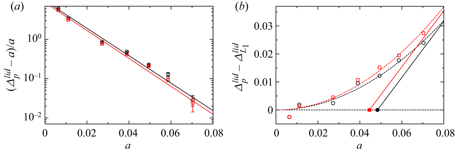
The deviation  $\varDelta _{p}^{lid} - \varDelta _{L_1}^{lid}$ between the minimal distance $\varDelta _{p}^{lid}$ of the trajectory of a neutrally buoyant particle from the moving wall and the minimum distance $\varDelta _{L_1}^{lid}$ from the moving wall of the closed streamline $L_1$ is shown in figure 28(b) as function of the particle radius $a$ (open symbols). Except for very small $a$, the limit cycle is always found to be further away from the wall than the closed streamline. The model of Hofmann & Kuhlmann (Reference Hofmann and Kuhlmann2011) considers perfectly advected particles that interact only with the boundary through inelastic contacts in the direction normal to the boundary. Their model predicts a stable limit cycle when the particle radius $a > a^* := \varDelta _{L_1}^{lid}$ is larger than the distance of the closed streamline from the boundary (filled symbols in figure 28b). Moreover, for $a > a^*$, the distance of the limit cycle from the boundary is $\varDelta _{p}^{lid} = a$, because the particle makes contact upon each return. For $a < a^*$, a quasi-periodic attractor is predicted. Thus within their model, contact with the boundary is made when $\varDelta _{p}^{lid} - \varDelta _{L_1}^{lid} = a-a^*$ (solid line in figure 28a). For large particle size, the experimental data seem to approach asymptotically the model prediction of Hofmann & Kuhlmann (Reference Hofmann and Kuhlmann2011). For $a< a^*$, however, the model of Hofmann & Kuhlmann (Reference Hofmann and Kuhlmann2011) fails to predict the observed limit cycle. The reason is particle–wall interaction forces that are not included in their model. These forces keep the particle further away from the wall and create a limit cycle instead of a quasi-periodic attractor. Within the range of particle radii investigated, the deviation $\varDelta _{p}^{lid} - \varDelta _{L_1}^{lid}$ can be approximated phenomenologically by a quadratic law (dashed lines). It must break down, however, for larger particle sizes for which the particle tends to make contact.
For weakly inertial particles, in the absence of the wall effect, limit cycles are expected to exist near closed streamlines of the flow, which can be either attractive or repelling, depending on the sign of  $|\varrho -1|$, the properties of the flow field, and the orientation of the buoyancy force (Wu et al. Reference Wu, Romanó and Kuhlmann2021). When the direction of the wall motion is collinear with the direction of the gravity vector, stable inertia-induced limit cycles were found to exist. In this case, we were able to separate the wall effect on the attraction rate from the period-one limit cycle P-1, using the results obtained for quasi-neutrally buoyant particles. The separation is based on the observation that both pure inertial and pure boundary-induced limit cycles are located very near the closed streamline $L_1$ such that both effects can be assumed to be additive. This assumption is motivated by both the inertia and wall effects on the particle trajectory being small near the stable limit cycle, both effects being essentially independent of each other, and each mechanism in isolation leads to a limit cycle which grows out of the same closed streamline of the set of KAM tori (for the wall effect, see Hofmann & Kuhlmann Reference Hofmann and Kuhlmann2011). Evidence for a superposition of the growth rates has been provided numerically by Romanò et al. (Reference Romanò, Kunchi Kannan and Kuhlmann2019a) and experimentally by Wu et al. (Reference Wu, Romanó and Kuhlmann2021). According to Hofmann & Kuhlmann (Reference Hofmann and Kuhlmann2011), limit cycles due to the particle–wall interaction are always stable. Consistently, we find that the wall effect enhances the attraction rate to the limit cycles. While the attraction rate due to inertia scales like $\sigma _i \sim (\varrho -1)\,{\textit {St}}$, the attraction rate in the presence of both inertia and wall effect does not exhibit a simple scaling. This is due to the dependence of the wall-induced attraction rate $\sigma _w(\textit {a})$ on the particle radius $a$ and on the character of the winding of the streamlines on the KAM tori (Hofmann & Kuhlmann Reference Hofmann and Kuhlmann2011; Wu et al. Reference Wu, Romanó and Kuhlmann2021).
In the case when the direction of the wall motion is reversed to be antiparallel to the gravity vector, inertial attractors for small inertia are replaced by inertial repellers. We find that the inertial repulsion from the unstable limit cycle dominates in the close vicinity of the limit cycle. The wall effect, however, stabilises the particle trajectory to a toroidal motion about the unstable limit cycle. Furthermore, by increasing the particle-to-fluid density ratio  $\varrho$, i.e. for stronger inertia and buoyancy, particle attractors with shape and position are found that differ significantly from any of the closed streamlines and KAM tori.
Tsorng et al. (Reference Tsorng, Capart, Lai and Young2006) have performed similar experiments using a water–glycerol mixture in a cubic cavity at  ${\textit {Re}}=470$ and a single density-matched particle with $a=0.015$. In their experiments, the viscous diffusion time was approximately $4.5$ min, and the observation time was typically 7 min. Different from our set-up, the gravity vector was directed perpendicular to the moving wall and into the liquid. The authors observed that the particle tends to move along preferential pathways, but did not find any attractors. The most likely explanation for the absence of attractors is the relatively large Reynolds number, since KAM structures are absent in the cubic cavity for ${\textit {Re}}=400$ and above (Romanò et al. Reference Romanò, Türkbay and Kuhlmann2020). While periodic attractors are conceptually possible also for pure chaotic streamlines (Kuhlmann & Muldoon Reference Kuhlmann and Muldoon2013), their existence is unlikely. Using the same apparatus, Tsorng et al. (Reference Tsorng, Capart, Lo, Lai and Young2008) extended the investigation to slightly heavy ( $\varrho \approx 1.0005$) and light ( $\varrho \approx 0.9993$) particles, where the density mismatch was achieved by variation of the composition of the water–glycerol mixture, keeping the temperature constant. They likewise report preferential pathways, but no attractors. While the reason seems to be again the absence of KAM structures for most of the Reynolds numbers ( $>400$) considered, they did not find attractors even for ${\textit {Re}}=130$. Possibly, the observation time was too short to be able to detect the attractors expected for ${\textit {Re}}=130$. Furthermore, the driving of the flow with a conveyor belt might have introduced disturbances to the flow larger than the present rotating cylinders.
The present results have elucidated the roles of flow structure, particle–boundary interaction, inertia and buoyancy forces for the existence and properties of particle attractors in the lid-driven cuboid. The fundamental results obtained are expected to help an improved understanding of multiphase systems, in particular on the microscale, in which similar phenomena arise. A dedicated design of micro-flow systems based on shaping the flow topology and utilising the particle–boundary interaction may, moreover, lead to novel micro-flow particle handling devices.
Interesting extensions of the current work would be the simultaneous measurement of trajectories of several particles. This way, the particle–particle interaction could be studied, and its impact on their motion near single-particle attractors. For very small particles one may still observe many particles being attracted as e.g. in thermocapillary liquid bridges (Schwabe et al. Reference Schwabe, Mizev, Udhayasankar and Tanaka2007), in which case the notion of finite-size coherent structures (FSCS) would apply (Romanò et al. Reference Romanò, Kunchi Kannan and Kuhlmann2019a). Furthermore, better theoretical and numerical particle–boundary interaction models could be developed and tested based on the particle dynamics that we have found.
Acknowledgements
F.R. thanks H. Abdelaziz for post-processing the numerical flow field on which the figures of § 6.2 are based.
Funding
The authors acknowledge TU Wien Bibliothek for financial support through its Open Access Funding Programme.
Declaration of interests
The authors report no conflict of interest.


 Open access

