


1. Introduction
River outflows and their associated boundary fronts strongly influence the ocean and thermohaline circulation (Rahmstorf Reference Rahmstorf2003), where less dense freshwater flows entering higher-density oceanic waters generate movement across the globe. Freshwater input from rivers introduced by the Arctic Ocean has been found to slow the distribution of heat throughout the Northern Hemisphere (Holliday et al. Reference Holliday2020). Moreover, the mixing of ocean and coastal waters generated by outflow currents determines nutrient transport and the subsequent distribution of phytoplankton populations (Ajani et al. Reference Ajani, Davies, Eriksen and Richardson2020). Sun et al. (Reference Sun2022) specifically emphasise how complex interactions between different river flows affect the distribution of the phytoplankton community in coastal waters of South Korea. On a smaller scale, the Hawkesbury River estuary in Australia is a source of nutrient-dense waters transported by the river plume (Li et al. Reference Li, Roughan, Kerry and Rao2022), directly influencing the marine taxonomy of the river mouth. Wang et al. (Reference Wang, Zhao, Zhu, McWilliams, Galgani, Md Amin, Nakajima, Jiang and Chen2022) further note that coastal and estuarine fronts led by river discharges are responsible for the accumulation of pollutants and microplastics.
Growing evidence relates increasing river discharge to rising coastal sea levels, as currents can be trapped along the coast. With the intensifying hydrological cycle (Pratap & Markonis Reference Pratap and Markonis2022), Tao et al. (Reference Tao, Tian, Ren, Yang, Yang, He, Cai and Lohrenz2014) predict up to a 60 % increase in discharge from the Mississippi River basin over the next century, the largest source of water drainage from North America into the Atlantic Ocean. Piecuch et al. (Reference Piecuch, Bittermann, Kemp, Ponte, Little, Engelhart and Lentz2018) examine how variable river discharge influences oceanic circulation and how this contributes to rising sea levels on the United States East Coast. Furthermore, from Atlantic and Gulf coast data, they suggest that river discharge is responsible for up to 15 % of the annual sea-level variance.
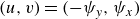
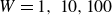
Winter sediment plumes from the Yangtze River spreading into the East China Sea forming a ‘shelf’ of water stretching leftwards (data from the MODIS satellite, 2017), made visible by tidal stirring of bottom sediments (Luo et al. Reference Luo, Zhu, Wu and Li2017).

Numerical studies of river outflows (Mestres et al. Reference Mestres, Sánchez-Arcilla and Sierra2007) examine how changes in river width, inlet transport and the Coriolis parameter affect the surface plume width given a constant outflow discharge. Tides, wind forcing and unsteady outflows can also influence the evolution of the coastal front (Southwick et al. Reference Southwick, Johnson and McDonald2017). In the Northern Hemisphere freshwater from rivers could be expected to turn right (in the direction of the Coriolis force). There are, however, clear indications of leftward propagation, such as the suspended sediments that form the Yangtze River plume front (figure 1). Johnson et al. (2017, JSM17 herein) capture both phenomena by using a theoretical long-wave approximation to the 1
 $ {1}/{2}$
-layer, quasigeostrophic (QG) equations where fluid expelled from a single-channel outflow is driven along the coast by a Kelvin wave (KW) and vortical advection. They use an idealised model where the current and upper layer have piecewise constant vorticity following the model by Pratt & Stern (Reference Pratt and Stern1986). This most closely applies to large-scale fronts that are governed by near-geostrophic dynamics (Nagai et al. Reference Nagai, Tandon and Rudnick2006) but remains useful in describing buoyant discharges by capturing much of the essential physics of gravity-current outflows where less dense fluid enters denser fluid, including for surface-advected buoyant estuarine outflows in the Hudson river (Chant et al. Reference Chant, Glenn, Hunter, Kohut, Chen, Houghton, Bosch and Schofield2008). Kubokawa (Reference Kubokawa1991) gives contour dynamics (CD) simulations that closely match the outflow gyre modes in the Tsugaru Strait. McCreary et al. (Reference McCreary, Zhang and Shetye1997) add entrainment and horizontally varying salinity, obtaining a 1
$ {1}/{2}$
-layer, quasigeostrophic (QG) equations where fluid expelled from a single-channel outflow is driven along the coast by a Kelvin wave (KW) and vortical advection. They use an idealised model where the current and upper layer have piecewise constant vorticity following the model by Pratt & Stern (Reference Pratt and Stern1986). This most closely applies to large-scale fronts that are governed by near-geostrophic dynamics (Nagai et al. Reference Nagai, Tandon and Rudnick2006) but remains useful in describing buoyant discharges by capturing much of the essential physics of gravity-current outflows where less dense fluid enters denser fluid, including for surface-advected buoyant estuarine outflows in the Hudson river (Chant et al. Reference Chant, Glenn, Hunter, Kohut, Chen, Houghton, Bosch and Schofield2008). Kubokawa (Reference Kubokawa1991) gives contour dynamics (CD) simulations that closely match the outflow gyre modes in the Tsugaru Strait. McCreary et al. (Reference McCreary, Zhang and Shetye1997) add entrainment and horizontally varying salinity, obtaining a 1
 $ {1}/{2}$
-layer ageostrophic model that contains the simplified model of Kubokawa (Reference Kubokawa1991) in the small Rossby number limit. Horner-Devine et al. (Reference Horner-Devine, Fong, Monismith and Maxworthy2006) and Thomas & Linden (Reference Thomas and Linden2007) model river plumes in the laboratory as coastal currents in geostrophic balance and note features like the upstream expanding bulge captured in the theory of JSM17 and Johnson (Reference Johnson2023). Gregorio et al. (Reference Gregorio, Thomas, Haidvogel, Taskinoglu and Skeen2011) repeat the experiments from Thomas & Linden (Reference Thomas and Linden2007), obtaining good agreement with numerical coastal outflow simulations (regional ocean modelling system, or ROMS) when horizontal viscous forces are small. These models consider buoyant outflows that are not in contact with the ocean floor and thus do not address the dynamics of outflows of fluid denser than the ambient which are strongly affected by bottom drag. The QG models also exclude internal waves involved in turbulent mixing when the outflow meets the ambient. If the fluid density differences are large then turbulent stresses can become important, particularly in sub-mesoscale fronts, although Pham & Sarkar (Reference Pham and Sarkar2019) still observe cold freshwater-carrying surface gravity currents, including those far from the coast, in the Bay of Bengal reminiscent of the laboratory experiments by Thomas & Linden (Reference Thomas and Linden2007). Mendes et al. (Reference Mendes, da Silva, Magalhaes, St-Denis, Bourgault, Pinto and Dias2021) note that such turbulence is unlikely to be important in the Duoro river plume where fluid density differences are small. More sophisticated two-layer outflow models describing the discharge of the Ganges-Brahmaputra-Meghna mega-delta (Kida & Yamazaki Reference Kida and Yamazaki2020), a major freshwater source in the Bay of Bengal, also show how fronts from the individual river branches that form the delta play an important role in the dynamics of the geostrophically balanced freshwater river plume.
$ {1}/{2}$
-layer ageostrophic model that contains the simplified model of Kubokawa (Reference Kubokawa1991) in the small Rossby number limit. Horner-Devine et al. (Reference Horner-Devine, Fong, Monismith and Maxworthy2006) and Thomas & Linden (Reference Thomas and Linden2007) model river plumes in the laboratory as coastal currents in geostrophic balance and note features like the upstream expanding bulge captured in the theory of JSM17 and Johnson (Reference Johnson2023). Gregorio et al. (Reference Gregorio, Thomas, Haidvogel, Taskinoglu and Skeen2011) repeat the experiments from Thomas & Linden (Reference Thomas and Linden2007), obtaining good agreement with numerical coastal outflow simulations (regional ocean modelling system, or ROMS) when horizontal viscous forces are small. These models consider buoyant outflows that are not in contact with the ocean floor and thus do not address the dynamics of outflows of fluid denser than the ambient which are strongly affected by bottom drag. The QG models also exclude internal waves involved in turbulent mixing when the outflow meets the ambient. If the fluid density differences are large then turbulent stresses can become important, particularly in sub-mesoscale fronts, although Pham & Sarkar (Reference Pham and Sarkar2019) still observe cold freshwater-carrying surface gravity currents, including those far from the coast, in the Bay of Bengal reminiscent of the laboratory experiments by Thomas & Linden (Reference Thomas and Linden2007). Mendes et al. (Reference Mendes, da Silva, Magalhaes, St-Denis, Bourgault, Pinto and Dias2021) note that such turbulence is unlikely to be important in the Duoro river plume where fluid density differences are small. More sophisticated two-layer outflow models describing the discharge of the Ganges-Brahmaputra-Meghna mega-delta (Kida & Yamazaki Reference Kida and Yamazaki2020), a major freshwater source in the Bay of Bengal, also show how fronts from the individual river branches that form the delta play an important role in the dynamics of the geostrophically balanced freshwater river plume.
Jamshidi & Johnson (Reference Jamshidi and Johnson2019, JJ19 herein) extend JSM17 to order-unity Rossby numbers using the semigeostrophic equations to investigate the validity of the QG approximation. The extension admits a KW propagating along the coast at a finite speed contrasting with the QG limit where the KW propagates infinitely fast. Even at Rossby numbers of order unity, the outflow behaviour remains qualitatively similar: the KW simply sets the boundary condition for the more slowly moving vortical fluid, as noted in § 2. We thus continue with the simpler QG model of JSM17, but capture more detail in the solutions by studying the dispersivepotential-vorticity(PV) equation which adds higher-order terms to the leading-order hydraulic PV equation. The dispersive equation captures the dynamics of the frontal waves that appear on the edge of the outflow current in the full CD integrations, but are necessarily absent in the hydraulic theory of JSM17, and also the compound-wave structures (described in § 4.2) seen in the CD integrations there. The dispersive equation predicts new behaviour such as the formation of dispersive-shock waves (DSWs) and wall-bounded wavetrains, not seen in the limited number of CD integrations in JSM17 but found in the CD integrations here, indicating a dynamical regime where coastal outflows might break into eddy trains. Perhaps the most important result is the demonstration that, in certain parameter regimes, the width of the coastal current cannot be determined uniquely from global quantities like the volume flux, PV and density contrast: the width also depends on the details on the geometry of the outflow, which appears below simply as the width of the outflow relative to the current width. Although a local theory can predict the balance in the current, the width of the current varies with the width of the outflow even when the global quantities are unchanged. The analysis builds on the methods in Jamshidi & Johnson (Reference Jamshidi and Johnson2020, JJ20 herein) who derive the dispersive equation for a coastal current of constant flux along a wall and analyse the Riemann problem for the adjustment of a step change in the width of an alongshore current using El’s dispersive-shock fitting technique (El Reference El2005).
Section 2 describes the idealised flow geometry considered here, governed by the
 $1{1}/{2}$
-QG equations, and presents the leading-order hydraulic limit of the equations and their first-order dispersive correction. Away from the source, the system supports travelling waves of fixed form and the equations governing these are noted in § 2.3. The flow evolves to divide naturally at large times into three regimes: a steady region containing the outflow, constant-width currents leading away from the outflow regions and unsteady propagating frontal regions leading the constant-width currents. Section 3 considers the outflow region, presenting numerical solutions for the asymptotically steady flow there and discussing the transition between subcritical and supercritical flow across the outflow. The widths of the outflow currents for negative PV outflows are shown to depend strongly on the strength of the dispersion. Section 4 describes the various compound-wave structures observed in the fronts leading the constant-width currents, and § 5 compares predictions from the dispersive long-wave theory with integrations of the full QG equations. The results are summarised briefly in § 6.
$1{1}/{2}$
-QG equations, and presents the leading-order hydraulic limit of the equations and their first-order dispersive correction. Away from the source, the system supports travelling waves of fixed form and the equations governing these are noted in § 2.3. The flow evolves to divide naturally at large times into three regimes: a steady region containing the outflow, constant-width currents leading away from the outflow regions and unsteady propagating frontal regions leading the constant-width currents. Section 3 considers the outflow region, presenting numerical solutions for the asymptotically steady flow there and discussing the transition between subcritical and supercritical flow across the outflow. The widths of the outflow currents for negative PV outflows are shown to depend strongly on the strength of the dispersion. Section 4 describes the various compound-wave structures observed in the fronts leading the constant-width currents, and § 5 compares predictions from the dispersive long-wave theory with integrations of the full QG equations. The results are summarised briefly in § 6.
2. Formulation
A schematic of a river outflow expelling fluid at
 $t\gt 0$
from an inlet with depth
$t\gt 0$
from an inlet with depth
 $D_{s}$
into the upper layer of depth
$D_{s}$
into the upper layer of depth
 $D$
. The lower layer of ambient ocean water below has infinite depth hence
$D$
. The lower layer of ambient ocean water below has infinite depth hence
 $\mathit{\Pi ^{\star }}=0$
. The subsequent displacement of the interface between the layers is denoted by
$\mathit{\Pi ^{\star }}=0$
. The subsequent displacement of the interface between the layers is denoted by
 $h$
. (a) The plan view of a river source of half-width
$h$
. (a) The plan view of a river source of half-width
 $L$
where the expelled fluid evolves to form a region
$L$
where the expelled fluid evolves to form a region
 $\mathcal{D}$
enclosed by a closed coastal front
$\mathcal{D}$
enclosed by a closed coastal front
 $\mathcal{C}$
(including the coast boundary
$\mathcal{C}$
(including the coast boundary
 $y=0$
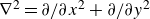
). (b) The side view where (b)(i): the outflow depth is deeper than the river inlet, so there is positive PVa generation. (b)(ii): outflow depth is shallower than the inlet (due to the presence of a shoal say) so there is negative PVa generation.
$y=0$
). (b) The side view where (b)(i): the outflow depth is deeper than the river inlet, so there is positive PVa generation. (b)(ii): outflow depth is shallower than the inlet (due to the presence of a shoal say) so there is negative PVa generation.

We consider a river outflow model where fluid is released from a constant depth inlet and flows along the coast into a half-space consisting of an upper active layer, comprising the expelled fluid and displaced ambient ocean water, and an ambient lower layer of infinite depth. The flow geometry is shown from a plan view in figure 2(a) and a side view in figures 2(b)(i), 2(b)(ii). We take Cartesian coordinates
 $\mathcal{O}xyz$
, with
$\mathcal{O}xyz$
, with
 $x$
along the coast,
$x$
along the coast,
 $y$
offshore and
$y$
offshore and
 $z$
vertical. The system rotates with Coriolis parameter
$z$
vertical. The system rotates with Coriolis parameter
 $f$
about the
$f$
about the
 $z$
-axis. Here,
$z$
-axis. Here,
 $D_{s}$
denotes the depth of the inlet,
$D_{s}$
denotes the depth of the inlet,
 $D$
the depth of the upper ambient fluid and
$D$
the depth of the upper ambient fluid and
 $L$
the half-width of the outflow lying along a vertical coast
$L$
the half-width of the outflow lying along a vertical coast
 $y=0$
. We denote the connected region of the expelled fluid by
$y=0$
. We denote the connected region of the expelled fluid by
 $\mathcal{D}$
, bounded by the contour
$\mathcal{D}$
, bounded by the contour
 $\mathcal{C}$
which separates expelled fluid from the ambient. At times
$\mathcal{C}$
which separates expelled fluid from the ambient. At times
 $t\gt 0$
, fluid is released from the outflow into the half-space
$t\gt 0$
, fluid is released from the outflow into the half-space
 $y\gt 0$
with a constant discharge rate that is independent of the width of the source and constant non-zero PV denoted by
$y\gt 0$
with a constant discharge rate that is independent of the width of the source and constant non-zero PV denoted by
 $\Pi ^{\star}$
. The expelled and ambient fluid in the upper layer has density
$\Pi ^{\star}$
. The expelled and ambient fluid in the upper layer has density
 $\rho _{1}$
while the lower layer has zero PV and density
$\rho _{1}$
while the lower layer has zero PV and density
 $\rho _{2}\gt \rho _{1}$
, with
$\rho _{2}\gt \rho _{1}$
, with
 $|\rho _{1}-\rho _{2}|\ll \rho _{2}$
so the Boussinesq approximation is valid. This layered system satisfies the 1
$|\rho _{1}-\rho _{2}|\ll \rho _{2}$
so the Boussinesq approximation is valid. This layered system satisfies the 1
 ${1}/{2}$
-layer QG equations provided the relative depth change between the inlet and the active layer is small, i.e.
${1}/{2}$
-layer QG equations provided the relative depth change between the inlet and the active layer is small, i.e.
 $|D-D_{s}| \ll D$
. Typical velocities are small compared with the speed of long free-surface water waves, so the surface
$|D-D_{s}| \ll D$
. Typical velocities are small compared with the speed of long free-surface water waves, so the surface
 $z=0$
can be taken as effectively rigid with the dynamics restricted to the interface between the layers. The difference between the potential vorticity of the expelled fluid and the upper ambient fluid, defined as the PV anomaly (PVa),
$z=0$
can be taken as effectively rigid with the dynamics restricted to the interface between the layers. The difference between the potential vorticity of the expelled fluid and the upper ambient fluid, defined as the PV anomaly (PVa),
 $\Pi _{0}:=\Delta \Pi ^{\star}=f/D_{s}-f/D$
, is positive if the outflow depth is deeper than the inlet depth
$\Pi _{0}:=\Delta \Pi ^{\star}=f/D_{s}-f/D$
, is positive if the outflow depth is deeper than the inlet depth
 $D_{s}\lt D$
, or negative if
$D_{s}\lt D$
, or negative if
 $D_{s}\gt D$
. Herein (as in JJ20) we denote PVa as just PV for brevity.
$D_{s}\gt D$
. Herein (as in JJ20) we denote PVa as just PV for brevity.
The evolution of the vortical boundary
 $\mathcal{C}$
is governed by the equation for the conservation of QG PV and since the PV has constant magnitude the evolution is entirely determined by the instantaneous position of
$\mathcal{C}$
is governed by the equation for the conservation of QG PV and since the PV has constant magnitude the evolution is entirely determined by the instantaneous position of
 $\mathcal{C}$
. This allows the full, unapproximated evolution to be computed accurately using contour dynamics (§ 5, Dritschel Reference Dritschel1988). To derive a long-wave equation we restrict attention to flows where the coastal front
$\mathcal{C}$
. This allows the full, unapproximated evolution to be computed accurately using contour dynamics (§ 5, Dritschel Reference Dritschel1988). To derive a long-wave equation we restrict attention to flows where the coastal front
 $\mathcal{C}$
does not overturn and the current width can be written as
$\mathcal{C}$
does not overturn and the current width can be written as
 $y=Y(x,t)$
. This is true for gently propagating coastal fronts but the CD integrations § 5 suggest that overturning can occur, particularly for flows begun impulsively, and is discussed separately. The QG equations allow the introduction of a streamfunction
$y=Y(x,t)$
. This is true for gently propagating coastal fronts but the CD integrations § 5 suggest that overturning can occur, particularly for flows begun impulsively, and is discussed separately. The QG equations allow the introduction of a streamfunction
 \begin{equation} \psi (x,y,t)=\frac {g^{\prime}h(x,y,t)}{fQ_{0}}, \end{equation}
where
 $h(x,y,t)$
is the interface displacement. Here,
$h(x,y,t)$
is the interface displacement. Here,
 $Q_{0}$
is the area flux expelled by the outflow (with total volume
$Q_{0}$
is the area flux expelled by the outflow (with total volume
 $Q_{0}D$
),
$Q_{0}D$
),
 $g^{\prime}$
is the reduced gravity, with the horizontal velocities of the flow given by
$g^{\prime}$
is the reduced gravity, with the horizontal velocities of the flow given by
 $(u, v) = (-\psi _{y}, \psi _{x})$
. Spatial and temporal scales are non-dimensionalised (with choices justified, along with other quantities below, in JSM17) according to the vortex length
$(u, v) = (-\psi _{y}, \psi _{x})$
. Spatial and temporal scales are non-dimensionalised (with choices justified, along with other quantities below, in JSM17) according to the vortex length
 $L_{v}$
and advection time scale
$L_{v}$
and advection time scale
 $T_{v}$
where
$T_{v}$
where
 \begin{equation} L_{v}=(Q_{0}/|\mathit{\Pi _{0}}D|)^{1/2}, \quad \quad T_{v}=L_{v}^2/Q_{0}. \end{equation}
We define
 $W$
to be the non-dimensionalised half-width (herein just width) of the outflow such that
$W$
to be the non-dimensionalised half-width (herein just width) of the outflow such that
 $W=L/L_{v}$
. The non-dimensional governing equation becomes
$W=L/L_{v}$
. The non-dimensional governing equation becomes
 \begin{equation} q=\nabla ^2 \psi - \frac {1}{a^2}\psi = \begin{cases} 0 & y \gt Y(x,t) \\ \mathit{\Pi } & 0 \lt y \lt Y(x,t), \end{cases} \end{equation}
where
 $\nabla ^2=\partial /\partial x^2+\partial /\partial y^2$
is the Laplacian operator, the constant PV is non-dimensionalised as
$\nabla ^2=\partial /\partial x^2+\partial /\partial y^2$
is the Laplacian operator, the constant PV is non-dimensionalised as
 $\mathit{\Pi }=\mathit{\Pi }_{0}/|\mathit{\Pi }_{0}|$
so that
$\mathit{\Pi }=\mathit{\Pi }_{0}/|\mathit{\Pi }_{0}|$
so that
 $\mathit{\Pi }$
gives the sign of the expelled PV and
$\mathit{\Pi }$
gives the sign of the expelled PV and
 $a = L_{R}/L_{v}$
is the ratio of the Rossby radius of deformation for the interface
$a = L_{R}/L_{v}$
is the ratio of the Rossby radius of deformation for the interface
 $L_{R}=\sqrt {g^{\prime}H}/f$
to the vortical length scale
$L_{R}=\sqrt {g^{\prime}H}/f$
to the vortical length scale
 $L_{v}$
. The parameter
$L_{v}$
. The parameter
 $a$
is later referred to as simply the Rossby radius. It measures the ratio of the strength of advection by the image vorticity to that by the KW induced flow. The jump in vorticity across
$a$
is later referred to as simply the Rossby radius. It measures the ratio of the strength of advection by the image vorticity to that by the KW induced flow. The jump in vorticity across
 $y=Y(x,t)$
, i.e. the material line
$y=Y(x,t)$
, i.e. the material line
 $\mathcal{C}$
, supports a frontal Rossby wave that propagates unidirectionally with high PV to its right and so in the same direction as the flow induced by the image, in the coastal wall, of the vortical current. Thus for
$\mathcal{C}$
, supports a frontal Rossby wave that propagates unidirectionally with high PV to its right and so in the same direction as the flow induced by the image, in the coastal wall, of the vortical current. Thus for
 $\mathit{\Pi } = +1$
, the frontal Rossby wave and advection by image vorticity combine with the KW to reinforce the rightward turning flow. For
$\mathit{\Pi } = +1$
, the frontal Rossby wave and advection by image vorticity combine with the KW to reinforce the rightward turning flow. For
 $\mathit{\Pi } = -1$
, the frontal Rossby wave and the image vorticity advection oppose the KW.
$\mathit{\Pi } = -1$
, the frontal Rossby wave and the image vorticity advection oppose the KW.
We denote the flux function of the source outflow by
 $Q(x)$
with width
$Q(x)$
with width
 $W$
along the coast
$W$
along the coast
 $y=0$
. The fluid is impulsively expelled at
$y=0$
. The fluid is impulsively expelled at
 $t\gt 0$
given by the no-flux boundary condition (2.4), and far from the coast the fluid is stationary so
$t\gt 0$
given by the no-flux boundary condition (2.4), and far from the coast the fluid is stationary so
 \begin{align} \psi (x,0,t) = Q(x), \end{align}
 \begin{align} \quad \psi \to 0, \quad y \to \infty . \end{align}
Here,
 $Q(x \leqslant -W)=0, \ Q(x \geqslant W)=1$
(so the area flux expelled is
$Q(x \leqslant -W)=0, \ Q(x \geqslant W)=1$
(so the area flux expelled is
 $1$
normalised from
$1$
normalised from
 $Q_{0}$
). JSM17 and JJ20 show that the asymmetry in
$Q_{0}$
). JSM17 and JJ20 show that the asymmetry in
 $Q(x)$
arises necessarily from the KW generated when the source is switched on. The KW propagates to the right at finite speed in JJ20 and instantaneously in JSM17 to set the coastal boundary condition.
$Q(x)$
arises necessarily from the KW generated when the source is switched on. The KW propagates to the right at finite speed in JJ20 and instantaneously in JSM17 to set the coastal boundary condition.
The remaining condition is the kinematic boundary condition that fluid particles on the coastal front remain on the coastal front
 $\mathcal{C}$
 \begin{align} Y_{t} = [\psi (x, Y(x,t))]_{x}. \end{align}
2.1. The leading-order hydraulic solution
Rescaling (2.3) using the long-wave variables
 \begin{align} X= \varepsilon x, \quad T= \varepsilon t, \end{align}
where
 $\varepsilon = 1/W$
, and expanding
$\varepsilon = 1/W$
, and expanding
 $\psi$
in terms of
$\psi$
in terms of
 $\varepsilon$
gives
$\varepsilon$
gives
 \begin{equation} \psi (X, y, T) = \psi ^{0}+\varepsilon ^2 \psi ^{1} + \mathcal{O}(\varepsilon ^4). \end{equation}
We substitute (2.8) into (2.3) which is matched with the leading-order
 $\varepsilon ^{0}$
and first-order
$\varepsilon ^{0}$
and first-order
 $\varepsilon ^{2}$
terms. This derivation is summarised from JJ20, with the modification that
$\varepsilon ^{2}$
terms. This derivation is summarised from JJ20, with the modification that
 $Q(x)$
here varies instead of being constant in
$Q(x)$
here varies instead of being constant in
 $x$
. Directly evaluating
$x$
. Directly evaluating
 $\psi ^{0}$
at the coastal front
$\psi ^{0}$
at the coastal front
 $y=Y(X,T)$
gives
$y=Y(X,T)$
gives
 \begin{equation} \psi ^{0}(X, Y, T) = Q_{e}(X, Y, T) = -\frac {a^2 \mathit{\Pi }}{2}+(Q(X)+a^2 \mathit{\Pi })e^{-Y/a}-\frac {\mathit{\Pi } a^2}{2}e^{-2Y/a}. \end{equation}
The parameter
 $Q_{e}(X, Y, T)$
gives the net rightward flux of the oceanic fluid at
$Q_{e}(X, Y, T)$
gives the net rightward flux of the oceanic fluid at
 $X$
with
$X$
with
 $Q(X)-Q_{e}(X,T)$
giving the net rightward flux in the coastal current. The kinematic boundary condition (2.6) at the leading order becomes, in terms of
$Q(X)-Q_{e}(X,T)$
giving the net rightward flux in the coastal current. The kinematic boundary condition (2.6) at the leading order becomes, in terms of
 $x$
and
$x$
and
 $t$
,
$t$
,
 \begin{equation} Y_{t}+\left [\left (\frac {Q(x)}{a}+a\mathit{\Pi }\right )e^{-Y/a}-a\mathit{\Pi }e^{-2Y/a}\right ]Y_{x}+Q^{\prime}(x)e^{-Y/a}=0. \end{equation}
Equation (2.10) is a first-order nonlinear partial differential equation (PDE) with disturbance propagation speed
 $C(Y)$
given by
$C(Y)$
given by
 \begin{equation} C(Y)=\left (\frac {Q(x)}{a}+a\mathit{\Pi }\right )e^{-Y/a}-a\mathit{\Pi }e^{-2Y/a}, \end{equation}
governing the leading-order behaviour of the coastal front
 $Y(x,t)$
. At each
$Y(x,t)$
. At each
 $x$
the disturbance speed
$x$
the disturbance speed
 $C(Y)$
is the sum of the frontal Rossby-wave speed and the fluid speed at the front. Information travels to the right when
$C(Y)$
is the sum of the frontal Rossby-wave speed and the fluid speed at the front. Information travels to the right when
 $C(Y)\gt 0$
and to the left when
$C(Y)\gt 0$
and to the left when
 $C(Y)\lt 0$
. This behaviour is directly analogous to the hydraulic behaviour in free-surface channel flow and has been described as Rossby-wave hydraulics (see, for example, Johnson & Clarke Reference Johnson and Clarke2001). Since the frontal Rossby wave is the sole wave present, solutions of (2.10) will be described simply as hydraulic solutions.
$C(Y)\lt 0$
. This behaviour is directly analogous to the hydraulic behaviour in free-surface channel flow and has been described as Rossby-wave hydraulics (see, for example, Johnson & Clarke Reference Johnson and Clarke2001). Since the frontal Rossby wave is the sole wave present, solutions of (2.10) will be described simply as hydraulic solutions.
2.2. The dispersive correction
The next order in
 $\varepsilon$
gives the
$\varepsilon$
gives the
 $\mathcal{O}(\varepsilon ^2)$
correction to
$\mathcal{O}(\varepsilon ^2)$
correction to
 $\psi$
on
$\psi$
on
 $y=Y(X,T)$
as
$y=Y(X,T)$
as
 \begin{align} \psi ^{1}(X,Y,T) & = -\frac {a^3 \mathit{\Pi }}{4}Y_{XX}+\left (\frac {a^2}{2}\mathit{\Pi }Y Y_{XX}+\frac {a^3}{4}\mathit{\Pi }Y_{XX}-\frac {a \mathit{\Pi }}{2}Y (Y_{X})^2 \right )e^{-2Y/a} \notag \\ &\quad +\frac {a}{2}Q_{XX}(X)Ye^{-Y/a}. \end{align}
The dispersive kinematic boundary condition (2.6) including these dispersive terms becomes
 \begin{align} &Y_{t}+\left [\frac {a^2 \mathit{\Pi }}{2}e^{-2Y/a}-\left (Q(x)+a^2\mathit{\Pi }\right )e^{-Y/a}\right ]_{x} +\frac {a^3\mathit{\Pi }}{4}Y_{xxx}\nonumber \\ &\quad -\mathit{\Pi }\left [\left (\frac {a^2}{2}YY_{xx}-\frac {a}{2}Y(Y_{x})^2+\frac {a^3}{4}Y_{xx}\right )e^{-2Y/a}\right ]_{x} -\left [\frac {a}{2}Q_{xx}(x)Ye^{-Y/a}\right ]_{x}=0. \end{align}
Expanding (2.13) gives the alternative form of the dispersive kinematic boundary condition
 \begin{align} &Y_{t}+\left [\left (\frac {Q(x)}{a}+a\mathit{\Pi }\right )e^{-Y/a}-a\mathit{\Pi }e^{-2Y/a}\right ]Y_{x} \notag \\ &\quad +\frac {a^3\mathit{\Pi }}{4}Y_{xxx}-\mathit{\Pi }\left ((Y-a/2)(Y_{x})^3+\frac {a^3}{4}Y_{xxx}+\frac {a^2}{2}YY_{xxx}-2aYY_{x}Y_{xx}\right )e^{-2Y/a}\notag \\ &\quad -Q_{x}(x)e^{-Y/a}-\frac {a}{2}Q_{xxx}(x)Ye^{-Y/a}-\frac {a}{2}Q_{xx}(x)\left (1-Y/a\right )Y_{x}e^{-Y/a}=0. \end{align}
While the parameter
 $\varepsilon$
no longer appears, the variables
$\varepsilon$
no longer appears, the variables
 $x, t$
vary slowly. Formally, this means
$x, t$
vary slowly. Formally, this means
 $1/\varepsilon \equiv W \gg 1$
and
$1/\varepsilon \equiv W \gg 1$
and
 $a$
is of order unity. When
$a$
is of order unity. When
 $Q(x)$
narrows to a point source outflow
$Q(x)$
narrows to a point source outflow
 $W \to 0$
, its derivatives become large
$W \to 0$
, its derivatives become large
 $Q_{x}(x) \sim 1/W \gg 1$
, which violates this requirement. The system can, however, still be treated with surprisingly good accuracy (§ 3.2).
$Q_{x}(x) \sim 1/W \gg 1$
, which violates this requirement. The system can, however, still be treated with surprisingly good accuracy (§ 3.2).
2.3. The travelling-wave solutions of the dispersive equation
In the regions
 $|x|\gt W$
, where the flux function is constant,
$|x|\gt W$
, where the flux function is constant,
 $Q(x) \equiv Q$
, the system supports waves of permanent form (see JJ20 for the case
$Q(x) \equiv Q$
, the system supports waves of permanent form (see JJ20 for the case
 $Q=1$
). We change to moving coordinates by setting
$Q=1$
). We change to moving coordinates by setting
 $\xi =x-st$
and look for solutions steady in this moving frame. The governing PV equation (2.14) can then be written in potential form
$\xi =x-st$
and look for solutions steady in this moving frame. The governing PV equation (2.14) can then be written in potential form
 \begin{equation} \left (Y_{\xi }\right )^2=\frac {2}{a^2}\frac {a^3e^{-2Y/a}-4a(Q\mathit{\Pi }+a^2)e^{-Y/a}+2s\mathit{\Pi }Y^2+\alpha Y + E}{a-(a+2Y)e^{-2Y/a}} \equiv \frac {2}{a^2} \frac {\nu (Y, s, \alpha , E)}{\mathcal{G}(Y)}, \end{equation}
where
 $\alpha , E$
are the constants of integration, and
$\alpha , E$
are the constants of integration, and
 $s$
is the speed of the travelling wave.
$s$
is the speed of the travelling wave.
JJ20 show that a solitary wave propagating along a background
 $Y=Y_{\infty }$
, with maximum displacement
$Y=Y_{\infty }$
, with maximum displacement
 $Y_1$
, satisfies
$Y_1$
, satisfies
 \begin{equation} \nu (Y=Y_{1}) = \nu (Y = Y_{\infty }) = \nu ^{\prime}(Y = Y_{\infty }) = 0, \end{equation}
where
 $^{\prime}$
denotes differentiation with respect to
$^{\prime}$
denotes differentiation with respect to
 $Y$
and a kink soliton joining two different far-field states
$Y$
and a kink soliton joining two different far-field states
 $Y_{1}$
and
$Y_{1}$
and
 $Y_{2}$
satisfies
$Y_{2}$
satisfies
 \begin{equation} \nu (Y=Y_{1}) = \nu (Y = Y_{2}) = \nu ^{\prime}(Y = Y_{1}) = \nu ^{\prime}(Y = {Y_{2}}) = 0. \end{equation}
For given external parameters
 $a, Q, \mathit{\Pi }$
, the kink soliton solution also determines a unique coastal intrusion where a current of constant width
$a, Q, \mathit{\Pi }$
, the kink soliton solution also determines a unique coastal intrusion where a current of constant width
 $Y_{1}=Y_{I}$
terminates at the coast so
$Y_{1}=Y_{I}$
terminates at the coast so
 $Y_{2}=0$
. Equation (2.17) determines the constants
$Y_{2}=0$
. Equation (2.17) determines the constants
 $\alpha , E$
, giving the unique intrusion speed
$\alpha , E$
, giving the unique intrusion speed
 $s_{I}$
and width
$s_{I}$
and width
 $Y_{I}$
,
$Y_{I}$
,
 \begin{align} (-a^2Y_{I}& +3a^3+4aQ\mathit{\Pi }-2Q\mathit{\Pi }Y_{I})e^{2Y_{I}/a}-(2a^2Y_{I}+4a^3+4aQ\mathit{\Pi }+2Q\mathit{\Pi }Y_{I})e^{Y_{I}/a}\notag \\ & +(a^2Y_{I}+a^3)=0, \end{align}
 \begin{align} & \qquad \quad s_{I}= \frac {-2a^2e^{-2Y_{I}/a}+4(a^2+Q\mathit{\Pi })e^{-Y_{I}/a}-2a^2-4Q\mathit{\Pi }}{-4Y_{I}\mathit{\Pi }}. \end{align}
Since
 $\mathcal{G}, \mathcal{G}^{\prime} \to 0$
as
$\mathcal{G}, \mathcal{G}^{\prime} \to 0$
as
 $Y \to 0$
, and
$Y \to 0$
, and
 $\nu , \nu ^{\prime} \to 0$
by construction, the PV front meets the coast with finite gradient
$\nu , \nu ^{\prime} \to 0$
by construction, the PV front meets the coast with finite gradient
 \begin{equation} (Y_{\xi })^2|_{Y=0}=\frac {2\mathit{\Pi }(as_{I}-Q)}{a^2}. \end{equation}
Intrusion solutions are shown below to play a significant role in determining the long time behaviour of solutions in certain parameter regimes. A closely related wave type, not present in JJ20, that appears in the outflow problem is a wall-bounded wavetrain. These waves are discussed in detail in § 4.5 and satisfy conditions given by (4.15).
3. The outflow region
As in the hydraulic solutions of JSM17, the outflow region controls the development of the solutions both upstream and downstream and so is considered here first. We consider initially the case
 $\mathit{\Pi }=-1$
, addressing the case
$\mathit{\Pi }=-1$
, addressing the case
 $\mathit{\Pi }=+1$
in § 3.1.2. For steady flow, (2.6) integrates directly to give
$\mathit{\Pi }=+1$
in § 3.1.2. For steady flow, (2.6) integrates directly to give
 \begin{equation} F(Y, Y_{x}, Y_{xx}) :=\psi ^{0}(x,Y)+\psi ^{1}(x,Y, Y_{x}, Y_{xx})=\Phi , \end{equation}
for some constant
 $\Phi$
, to be determined. As
$\Phi$
, to be determined. As
 $x \to \pm \infty$
, the PV front settles to constant-width currents of upstream width
$x \to \pm \infty$
, the PV front settles to constant-width currents of upstream width
 $Y_{-}$
and downstream width
$Y_{-}$
and downstream width
 $Y_{+}$
(say). The dispersive term is absent for constant-width currents and so both
$Y_{+}$
(say). The dispersive term is absent for constant-width currents and so both
 $Y_{-}$
and
$Y_{-}$
and
 $Y_{+}$
satisfy the hydraulic form of (3.1) which becomes, from (2.9),
$Y_{+}$
satisfy the hydraulic form of (3.1) which becomes, from (2.9),
 \begin{equation} \Phi = Q_e(Q=0,Y_-)=Q_e(Q=1,Y_+). \end{equation}
There are no stationary (
 $s=0$
) non-trivial solutions of (2.15) with
$s=0$
) non-trivial solutions of (2.15) with
 $Q=0$
and so the constant-width solution
$Q=0$
and so the constant-width solution
 $Y=Y_{-}$
extends to the downstream edge of the source region at
$Y=Y_{-}$
extends to the downstream edge of the source region at
 $x=-W$
. In
$x=-W$
. In
 $x\gt W$
, where
$x\gt W$
, where
 $Q=1$
, non-trivial stationary solitary waves solutions of (2.15) exist and the solution across the source region must match to part of one of these riding on the background
$Q=1$
, non-trivial stationary solitary waves solutions of (2.15) exist and the solution across the source region must match to part of one of these riding on the background
 $Y=Y_{+}$
. The problem for the flow in the source region can thus be posed as the boundary value problem (BVP)
$Y=Y_{+}$
. The problem for the flow in the source region can thus be posed as the boundary value problem (BVP)
 \begin{align} \quad &Y=Y_{-}; \quad x\leqslant -W, \end{align}
 \begin{align} \quad &\psi ^{0}(x,Y)+\psi ^{1}(x,Y, Y_{x}, Y_{xx})=\Phi ; \quad |x| \leqslant W \end{align}
 \begin{align} \quad &(Y_{x})^2=\frac {2}{a^2}\frac {\nu (Y, \alpha _{+}, E_{+})}{\mathcal{G}(Y)}; \quad x \geqslant W, \end{align}
with
 $Y$
and
$Y$
and
 $Y_x$
continuous across
$Y_x$
continuous across
 $x=\pm W$
.
$x=\pm W$
.
The constants
 $\alpha _{+}, E_{+}$
are determined using the conditions for the existence of a soliton with
$\alpha _{+}, E_{+}$
are determined using the conditions for the existence of a soliton with
 $\mathit{\Pi }=-1$
, lying on
$\mathit{\Pi }=-1$
, lying on
 $Y=Y_{+}$
, in (2.16), and solving (3.4) in the outflow region
$Y=Y_{+}$
, in (2.16), and solving (3.4) in the outflow region
 $|x| \leqslant W$
gives the value of
$|x| \leqslant W$
gives the value of
 $Y(W) \equiv Y_{+}$
and
$Y(W) \equiv Y_{+}$
and
 $\Phi$
, allowing (3.5) to be solved from
$\Phi$
, allowing (3.5) to be solved from
 $x=W$
. Knowledge of
$x=W$
. Knowledge of
 $\Phi$
uniquely determines the widths of the far-field
$\Phi$
uniquely determines the widths of the far-field
 $Y_{+}, Y_{-}$
and, by extension, the entire steady system.
$Y_{+}, Y_{-}$
and, by extension, the entire steady system.
We solve this system by truncating the domain at some
 $x= \pm L$
for large
$x= \pm L$
for large
 $L$
and using a BVP solver (bvp4c/bvp5c) in MATLAB. Equation (3.4) is solved across the entire domain, setting the flux function to be
$L$
and using a BVP solver (bvp4c/bvp5c) in MATLAB. Equation (3.4) is solved across the entire domain, setting the flux function to be
 $Q(x):=Q_{4}(x)$
in (4.1), which is equivalent to solving (3.3), (3.4), (3.5) separately in each domain and unifying the solutions. Although a shooting method can be used to find
$Q(x):=Q_{4}(x)$
in (4.1), which is equivalent to solving (3.3), (3.4), (3.5) separately in each domain and unifying the solutions. Although a shooting method can be used to find
 $\Phi$
similarly to Jamshidi & Johnson (Reference Jamshidi and Johnson2021), the bvp4c/bvp5c solvers handle this automatically on introducing the auxiliary equation
$\Phi$
similarly to Jamshidi & Johnson (Reference Jamshidi and Johnson2021), the bvp4c/bvp5c solvers handle this automatically on introducing the auxiliary equation
 \begin{equation} \Phi =Q_{e}(x=-W)=\frac {-a^2\mathit{\Pi }}{2}+(Q+a^2\mathit{\Pi })e^{-Y_{-}/a}-\frac {\mathit{\Pi }a^2}{2}e^{-2Y_{-}/a}, \end{equation}
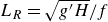
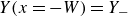
to be satisfied alongside the ordinary differential equation (ODE). Figure 3 shows the frontal position and streamlines for a typical solution. The entire outflow leaves the source and turns upstream, travelling to an unsteady upstream frontal region in the full problem where some of the fluid turns to form a downstream return current along the PV front. This leaves a central recirculating region just downstream of the outflow, as observed in the experiments of Thomas & Linden (Reference Thomas and Linden2007) and the ageostrophic integrations of Gregorio et al. (Reference Gregorio, Thomas, Haidvogel, Taskinoglu and Skeen2011) and modelled in Johnson (Reference Johnson2023). The Rossby frontal wave travels upstream with high PV to its right. Its speed precisely equals the coastal current speed at the dispersive control point, marked as a blue dot on the front, where
 $C(Y)=0$
. Upstream of this point
$C(Y)=0$
. Upstream of this point
 $C(y)\lt 0$
and the flow is subcritical, with information propagating upstream. Downstream of this point
$C(y)\lt 0$
and the flow is subcritical, with information propagating upstream. Downstream of this point
 $C(y)\gt 0$
and the flow is supercritical, with information propagating downstream. This identification of hydraulic regimes is justified in the following section.
$C(y)\gt 0$
and the flow is supercritical, with information propagating downstream. This identification of hydraulic regimes is justified in the following section.
The streamlines (blue) and of a steady dispersive solution with
 $a=1.3, \mathit{\Pi }=-1$
, and source lying within
$a=1.3, \mathit{\Pi }=-1$
, and source lying within
 $|x|\leqslant W=3$
. The streamline coinciding with the coastal front
$|x|\leqslant W=3$
. The streamline coinciding with the coastal front
 $Y(x)$
is marked in black. The dispersive control point where
$Y(x)$
is marked in black. The dispersive control point where
 $C(Y)$
vanishes is shown by a blue circle. The blue-dashed streamline
$C(Y)$
vanishes is shown by a blue circle. The blue-dashed streamline
 $\psi =1$
bounds a region of recirculating flow.
$\psi =1$
bounds a region of recirculating flow.

3.1. Hydraulic control
Consider wavelike perturbations of a steady solution
 $Y = Y_{s}(x)$
of (2.14) of the form
$Y = Y_{s}(x)$
of (2.14) of the form
 \begin{equation} Y(x,t)=Y_{s}(x)+\hat {\varepsilon } y(x,t), \quad \hat {y} \sim \mathcal{O}(1), \end{equation}
where
 $\hat {\varepsilon } \ll 1$
. Then, to order
$\hat {\varepsilon } \ll 1$
. Then, to order
 $\hat {\varepsilon }$
, (2.14) becomes
$\hat {\varepsilon }$
, (2.14) becomes
 \begin{align} &\frac {\partial \hat {y}}{\partial t}+\hat {C}\frac {\partial \hat {y}}{\partial x}=f\left (\hat {y},\hat {y}_{xx}, \hat {y}_{xxx}\right ), \end{align}
 \begin{align} & \hat {C} = C(Y_{s})+C^{1}, \end{align}
 \begin{align} & C^{1} = -\mathit{\Pi }\left (3\left (Y_{s}-\frac {a}{2}\right )(Y_{s}^{\prime})^{2}-2aY_{s}Y_{s}^{\prime\prime}\right )e^{-2Y_{s}/a}-\frac {a}{2}Q^{\prime\prime}(x)\left (1-Y_{s}/a\right )e^{-Y_{s}/a}.\quad\, \end{align}
Both the forcing function
 $f$
and the wavespeed perturbation
$f$
and the wavespeed perturbation
 $C^{1}$
are of order
$C^{1}$
are of order
 $\varepsilon ^2$
and so (3.8) can be regarded, at leading order in the long-wave parameter
$\varepsilon ^2$
and so (3.8) can be regarded, at leading order in the long-wave parameter
 $\varepsilon$
, as a first-order PDE with disturbance propagation speed
$\varepsilon$
, as a first-order PDE with disturbance propagation speed
 $\hat {C}=C(Y)+\mathcal{O}(\varepsilon ^2)$
. As in the hydraulic limit,
$\hat {C}=C(Y)+\mathcal{O}(\varepsilon ^2)$
. As in the hydraulic limit,
 $C(Y)$
, given by (2.11), is the local speed of infinitesimal perturbations to the steady dispersive equation.
$C(Y)$
, given by (2.11), is the local speed of infinitesimal perturbations to the steady dispersive equation.
3.1.1. The
 $\mathit{\Pi }=-1$
case
$\mathit{\Pi }=-1$
case

The unsteady hydraulic solution (2.10) in JSM17 evolves to be critically controlled at the downstream edge
 $x_{c}=W$
of the source and thus sets
$x_{c}=W$
of the source and thus sets
 $Y_{+}$
and
$Y_{+}$
and
 $Y_{-}$
. In this case, (3.1) becomes
$Y_{-}$
. In this case, (3.1) becomes
 \begin{equation} Q_{e}(Y=Y_{-}, Q=0, \mathit{\Pi })=Q_{e}(Y=Y_{+}, Q=1, \mathit{\Pi }) = \Phi , \end{equation}
where
 $Q_{e} \equiv \psi ^{0}$
is the leading-order (hydraulic) streamfunction evaluated at the PV front. Requiring flow to be critically controlled gives some essential conditions in the hydraulic equation. From JSM17,
$Q_{e} \equiv \psi ^{0}$
is the leading-order (hydraulic) streamfunction evaluated at the PV front. Requiring flow to be critically controlled gives some essential conditions in the hydraulic equation. From JSM17,
 $Y_{+}$
is determined by setting the width at the downstream edge control point
$Y_{+}$
is determined by setting the width at the downstream edge control point
 $C(Y_{+})=0$
and
$C(Y_{+})=0$
and
 $Y_{-}$
can be derived using equation (3.11), giving
$Y_{-}$
can be derived using equation (3.11), giving
 \begin{equation} Y_{+} := (Y_{+})_{hyd, \ -1} = a\ln \left (\frac {a^2}{a^2-1}\right ), \quad Y_{-} :=(Y_{-})_{hyd, \ -1}=a\ln \left (\frac {a^4+a^2\sqrt {2a^2-1}}{(a^2-1)^2}\right ). \end{equation}
When
 $a \leqslant 1$
, these expressions fail and steady solutions no longer exist.
$a \leqslant 1$
, these expressions fail and steady solutions no longer exist.
As shown above, the control point for dispersive solutions also occurs when
 $C(Y)=0$
, however, as the dispersive solution differs from the hydraulic solution, the control point, although occurring at the same value of
$C(Y)=0$
, however, as the dispersive solution differs from the hydraulic solution, the control point, although occurring at the same value of
 $Y$
, lies at a different value of
$Y$
, lies at a different value of
 $x_c\neq W$
, which can only be determined once the dispersive solution is known. Since the control point is fixed at
$x_c\neq W$
, which can only be determined once the dispersive solution is known. Since the control point is fixed at
 $x_{c}=W$
in the hydraulic solutions the current widths
$x_{c}=W$
in the hydraulic solutions the current widths
 $Y_{-}, Y_{+}$
do not change with the outflow width. The current width in the dispersive solutions varies with the width of the outflow and so to does the position of the control point.
$Y_{-}, Y_{+}$
do not change with the outflow width. The current width in the dispersive solutions varies with the width of the outflow and so to does the position of the control point.
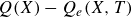
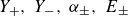
The steady dispersive solutions (shown in blue) for
 $a=1.3, \ \mathit{\Pi }=-1$
plotted for source widths: (a) W = 3, (b) W = 10 with the outflow centred at
$a=1.3, \ \mathit{\Pi }=-1$
plotted for source widths: (a) W = 3, (b) W = 10 with the outflow centred at
 $x=0$
(marked as a filled star). For comparison, the full QG solutions (in black) is shown for
$x=0$
(marked as a filled star). For comparison, the full QG solutions (in black) is shown for
 $t=500$
. The locations of the hydraulic and dispersive control points are shown by a black and blue filled circle, respectively. The red line denotes the hydraulic rarefaction at
$t=500$
. The locations of the hydraulic and dispersive control points are shown by a black and blue filled circle, respectively. The red line denotes the hydraulic rarefaction at
 $t=10\,000$
, an almost constant-width current extending from the hydraulic control point.
$t=10\,000$
, an almost constant-width current extending from the hydraulic control point.

Figure 4 compares the numerical steady dispersive solution with the full QG solution (using the contour dynamics method of § 5) run until
 $Y_{-}$
and
$Y_{-}$
and
 $Y_{+}$
converge to their steady values. The widths
$Y_{+}$
converge to their steady values. The widths
 $Y_{\pm }$
are well predicted for source widths
$Y_{\pm }$
are well predicted for source widths
 $W=3,10$
, significantly improving on the large-time limit of the downstream hydraulic rarefaction solution shown in red. The
$W=3,10$
, significantly improving on the large-time limit of the downstream hydraulic rarefaction solution shown in red. The
 $Y$
displacements of the hydraulic (black) and dispersive (blue) control points are the same, but the values of
$Y$
displacements of the hydraulic (black) and dispersive (blue) control points are the same, but the values of
 $x_c$
differ. The control point for
$x_c$
differ. The control point for
 $W=10$
lies closer to the downstream outflow than that for
$W=10$
lies closer to the downstream outflow than that for
 $W=3$
since the solution converges to the hydraulic solution as
$W=3$
since the solution converges to the hydraulic solution as
 $W$
increases.
$W$
increases.
3.1.2. The
$\mathit{\Pi }=+1$
case

Critical control in the hydraulic solution for
 $\mathit{\Pi }=+1$
occurs at the upstream edge of the source outflow at
$\mathit{\Pi }=+1$
occurs at the upstream edge of the source outflow at
 $x_c=-W$
giving a steady solution with no current upstream. For
$x_c=-W$
giving a steady solution with no current upstream. For
 $x\gt -W$
,
$x\gt -W$
,
 $C(Y)\gt 0$
, so the flow is supercritical everywhere. As shown in JSM17, this gives remarkably accurate results compared with the full problem, predicting the upstream and downstream steady current widths as
$C(Y)\gt 0$
, so the flow is supercritical everywhere. As shown in JSM17, this gives remarkably accurate results compared with the full problem, predicting the upstream and downstream steady current widths as
 \begin{equation} (Y_{-})_{hyd, \ +1} \equiv 0, \quad (Y_{+})_{hyd, \ +1}=a\ln \left (1/a^2+1 + \sqrt {1/a^4+2/a^2}\right ). \end{equation}
The dispersive equation also establishes a control point, but this causes the front to cross the coast, reaching negative
 $Y$
values, This invalidates the solutions and so comparison with the full problem is omitted. The dispersive PV equation improves on hydraulic solutions only for negative PV.
$Y$
values, This invalidates the solutions and so comparison with the full problem is omitted. The dispersive PV equation improves on hydraulic solutions only for negative PV.
3.2.
The narrow source limit,
$W \to 0$

The governing PV equation (2.14) is not formally valid for narrow outflows with
 $W \lesssim \mathcal{O}(1)$
. However, over long times, the dispersive equation for
$W \lesssim \mathcal{O}(1)$
. However, over long times, the dispersive equation for
 $\mathit{\Pi }=-1$
captures the far-field values
$\mathit{\Pi }=-1$
captures the far-field values
 $(Y_{-}, Y_{+})$
of the full problem well in this regime (figure 5). It is therefore useful to analyse the dispersive equation in this limit and extend the analysis of (2.14) to all
$(Y_{-}, Y_{+})$
of the full problem well in this regime (figure 5). It is therefore useful to analyse the dispersive equation in this limit and extend the analysis of (2.14) to all
 $W$
.
$W$
.
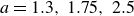
(a) The steady dispersive solutions (blue) at
 $a=1.3, \ \mathit{\Pi }=-1$
shown for different widths
$a=1.3, \ \mathit{\Pi }=-1$
shown for different widths
 $W=1, \ 10, 100$
, compared directly with the contour dynamics for
$W=1, \ 10, 100$
, compared directly with the contour dynamics for
 $W=0$
at
$W=0$
at
 $t=1000$
(shown in black). Also overlaid is the comparison (dotted lines) with the hydraulic and dispersive predictions of the current widths
$t=1000$
(shown in black). Also overlaid is the comparison (dotted lines) with the hydraulic and dispersive predictions of the current widths
 $(Y_{\pm })_{hyd}$
,
$(Y_{\pm })_{hyd}$
,
 $(Y_{\pm })_{W=0}$
. (b) As above but for
$(Y_{\pm })_{W=0}$
. (b) As above but for
 $a=1.75$
and
$a=1.75$
and
 $a=2.5$
(
$a=2.5$
(
 $W=1, \ 3, \ 10$
).
$W=1, \ 3, \ 10$
).

In the steady solutions for
 $\mathit{\Pi }=-1$
the far-field currents join through a (truncated) soliton which connects the downstream constant-width current
$\mathit{\Pi }=-1$
the far-field currents join through a (truncated) soliton which connects the downstream constant-width current
 $Y_{+}$
to an intermediate point
$Y_{+}$
to an intermediate point
 $Y=Y_{s}$
at
$Y=Y_{s}$
at
 $x=W$
that is subsequently linked smoothly across the outflow region
$x=W$
that is subsequently linked smoothly across the outflow region
 $|x|\lt W$
to the constant-width current
$|x|\lt W$
to the constant-width current
 $Y(x=-W) = Y_{-}$
. As shown in figure 5, for decreasing source widths the solution the cross-outflow matching becomes progressively steeper, approaching a vertical jump at
$Y(x=-W) = Y_{-}$
. As shown in figure 5, for decreasing source widths the solution the cross-outflow matching becomes progressively steeper, approaching a vertical jump at
 $x=0$
as
$x=0$
as
 $W\to 0$
. The soliton truncates at its maximum height to minimise the width of the jump. Figure 6 shows this suggested shape of the coastal front for a point source outflow. Thus we require that as
$W\to 0$
. The soliton truncates at its maximum height to minimise the width of the jump. Figure 6 shows this suggested shape of the coastal front for a point source outflow. Thus we require that as
 $W\to 0$
,
$W\to 0$
,
 $Y(x)$
satisfies
$Y(x)$
satisfies
 \begin{align} Y(x \to 0^{-})=Y_{-}, \quad Y(x \to 0^{+})=Y_{s}, \quad Y_{x}(x \to 0^{-})=0, \quad Y_{x}(x \to 0^{+})=0, \end{align}
with
 $Y_{s}$
giving the width from the coast of the soliton.
$Y_{s}$
giving the width from the coast of the soliton.
The suggested structure of the coastal front
 $\mathcal{C}$
for
$\mathcal{C}$
for
 $\mathit{\Pi }=-1$
as the outflow width
$\mathit{\Pi }=-1$
as the outflow width
 $W \to 0$
in dispersive flow. A shock links the constant-width current in
$W \to 0$
in dispersive flow. A shock links the constant-width current in
 $x\lt 0$
to a soliton asymptoting to
$x\lt 0$
to a soliton asymptoting to
 $Y_{+}$
.
$Y_{+}$
.

Integrating the steady form of (2.13) once gives
 \begin{align} \frac {a^{3} \mathit{\Pi }}{4} Y_{x x}-\mathit{\Pi } & {\left [\left (\frac {a^{2}}{2} Y Y_{x x}-\frac {a}{2} Y\left (Y_{x}\right )^{2}+\frac {a^{3}}{4} Y_{x x}\right ) e^{-2 Y / a}\right ]-\frac {a}{2} Q^{\prime \prime }(x) Y e^{-Y / a} } \notag \\ + & \frac {a^{2} \mathit{\Pi }}{2} e^{-2 Y / a}-\left (Q(x)+a^{2} \mathit{\Pi }\right ) e^{-Y / a}-\Phi =0, \end{align}
with constant of integration
 $\Phi =Q_{e}(Y_{-})$
. On integrating (3.15) across the outflow from
$\Phi =Q_{e}(Y_{-})$
. On integrating (3.15) across the outflow from
 $-W$
to
$-W$
to
 $W$
with respect to
$W$
with respect to
 $x$
, and taking the limit
$x$
, and taking the limit
 $W \rightarrow 0$
, the integral involving the last line of (3.15) vanishes as the integrand is bounded. Since
$W \rightarrow 0$
, the integral involving the last line of (3.15) vanishes as the integrand is bounded. Since
 $Y_{x}=0$
at
$Y_{x}=0$
at
 $x= \pm W$
from (3.14) the first term in the first line of (3.15) also vanishes. The remaining terms then give, after some simplification,
$x= \pm W$
from (3.14) the first term in the first line of (3.15) also vanishes. The remaining terms then give, after some simplification,
 \begin{align} \lim _{W \rightarrow 0} \int _{-W}^{W}\left \{\frac {\mathit{\Pi } a}{4}\left [(2 Y+a) e^{-2 Y / a}\right ] Y_{xx}+Q^{\prime \prime }(x) Y e^{-Y / a}\right \} \ {\textrm{d}}x=0. \end{align}
Now define the shock width, or jump in
 $Y(x)$
across
$Y(x)$
across
 $x=0$
, by
$x=0$
, by
 $\langle Y\rangle$
, so
$\langle Y\rangle$
, so
 \begin{equation} \langle Y\rangle =\lim _{W \rightarrow 0}[Y(W)-Y(-W)]=Y_{-}-Y_{s}, \end{equation}
and
 $\langle Q\rangle =1$
. Taking the indefinite integral of (3.15) from
$\langle Q\rangle =1$
. Taking the indefinite integral of (3.15) from
 $-W$
to
$-W$
to
 $x$
, integrating the result across the outflow from
$x$
, integrating the result across the outflow from
 $-W$
to
$-W$
to
 $W$
as
$W$
as
 $W \rightarrow 0$
, integrating by parts and simplifying using (3.16) gives
$W \rightarrow 0$
, integrating by parts and simplifying using (3.16) gives
 \begin{align} &\frac {a^{2} \mathit{\Pi }}{2}\langle Y\rangle +\frac {\mathit{\Pi } a^{2}}{4}\langle (Y+a) e^{-2 Y / a}\rangle \notag \\ &\qquad +\lim _{W \rightarrow 0} \int _{-W}^{W} x\left \{\frac {\mathit{\Pi } a}{4}\left [(2 Y+a) e^{-2 Y / a}\right ] Y_{xx}+Q^{\prime \prime }(x) Y e^{-Y / a}\right \} d x = 0. \end{align}
In the limit
 $W \rightarrow 0$
 \begin{equation} Y^{\prime \prime }(x) \rightarrow \langle Y\rangle \delta ^{\prime }(x), \quad Q^{\prime \prime }(x) \rightarrow \delta ^{\prime }(x), \end{equation}
where
 $\delta (x)$
is the Dirac delta function. Simplifying (3.18) then gives the required jump condition
$\delta (x)$
is the Dirac delta function. Simplifying (3.18) then gives the required jump condition
 \begin{align} \frac {a^{2} \mathit{\Pi }}{2}\langle Y\rangle +\frac {\mathit{\Pi } a^{2}}{4}\langle (Y+a) e^{-2 Y / a}\rangle -\frac {\mathit{\Pi } a}{4}\langle Y\rangle \left [(2 Y+a) e^{-2 Y / a}\right ]_{x=0}-\left [Y e^{-Y / a}\right ]_{x=0}=0, \end{align}
where for any
 $g(Y)$
, we define
$g(Y)$
, we define
 $[g(Y)]_{x=0}$
as
$[g(Y)]_{x=0}$
as
 \begin{equation} [g(Y)]_{x=0}=\left [g(Y_{-})+g(Y_{s})\right ] / 2. \end{equation}
We have the first equation (3.20) to solve for the three unknowns (
 $Y_{-}, Y_{s}, Y_{+}$
). Next, we introduce a steady soliton in the constant
$Y_{-}, Y_{s}, Y_{+}$
). Next, we introduce a steady soliton in the constant
 $Q=1$
region by imposing the conditions (2.16) derived from the travelling-wave solutions of the dispersive PV equation. We require that the soliton joins to
$Q=1$
region by imposing the conditions (2.16) derived from the travelling-wave solutions of the dispersive PV equation. We require that the soliton joins to
 $Y_{s} \neq Y_{+}$
, which gives the second equation
$Y_{s} \neq Y_{+}$
, which gives the second equation
 \begin{align} a^3e^{-2Y_{s}/a}-4a(a^2-1)e^{-Y_{s}/a}+\alpha _{+}Y_{s}+E_{+}=0, \end{align}
with the constants
 $\alpha _{+}, \ E_{+}$
determined from (2.16).
$\alpha _{+}, \ E_{+}$
determined from (2.16).
Since
 $Y_{+}, \ Y_{-}$
are linked by the hydraulic flux function
$Y_{+}, \ Y_{-}$
are linked by the hydraulic flux function
 $Q_{e}(Y)= \mathit{\Phi }$
, the final equation is given by
$Q_{e}(Y)= \mathit{\Phi }$
, the final equation is given by
 \begin{align} \frac {a^2}{2}+(1-a^2)e^{-Y_{+}/a}+\frac {a^2}{2}e^{-2Y_{+}/a}=\frac {a^2}{2}-a^2e^{-Y_{-}/a}+\frac {a^2}{2}e^{-2Y_{-}/a}=\mathit{\Phi }. \end{align}
Solving (3.20), (3.22), (3.23) simultaneously (and requiring
 $Y_{+} \leqslant Y_{s} \lt Y_{-}$
) gives the values of
$Y_{+} \leqslant Y_{s} \lt Y_{-}$
) gives the values of
 $(Y_{-}, Y_{+}, Y_{s})$
for
$(Y_{-}, Y_{+}, Y_{s})$
for
 $\mathit{\Pi }=-1$
. The shock solution is an unphysical artefact of the dispersive equation in the limit
$\mathit{\Pi }=-1$
. The shock solution is an unphysical artefact of the dispersive equation in the limit
 $W\to 0$
that, however, predicts the values of
$W\to 0$
that, however, predicts the values of
 $Y_{-}$
and
$Y_{-}$
and
 $Y_{+}$
found in the numerical solutions of the full problem.
$Y_{+}$
found in the numerical solutions of the full problem.
The steady hydraulic and dispersive
 $W \to 0$
width predictions give the upper or lower bounds of
$W \to 0$
width predictions give the upper or lower bounds of
 $Y_{\pm }$
for
$Y_{\pm }$
for
 $\mathit{\Pi }=-1$
such that
$\mathit{\Pi }=-1$
such that
 \begin{align} (Y_{-})_{W=0, \ -1}:=(Y_{-})_{max, \ -1}, \quad (Y_{-})_{hyd, \ -1}:=(Y_{-})_{min, \ -1} \notag \\ (Y_{+})_{W=0, \ -1}:=(Y_{+})_{min, \ -1}, \quad (Y_{+})_{hyd, \ -1}:=(Y_{+})_{max, \ -1}, \end{align}
where
 $hyd$
refers to the hydraulic predictions, giving an upper (
$hyd$
refers to the hydraulic predictions, giving an upper (
 $max$
) and lower bound (
$max$
) and lower bound (
 $min$
) to the steady current widths for some Rossby radius
$min$
) to the steady current widths for some Rossby radius
 $a$
. Figure 5 compares the numerical steady dispersive solutions for different
$a$
. Figure 5 compares the numerical steady dispersive solutions for different
 $W, \ a$
values for
$W, \ a$
values for
 $\mathit{\Pi }=-1$
with the theoretical current widths
$\mathit{\Pi }=-1$
with the theoretical current widths
 $Y_{\pm }$
. For small widths the upstream
$Y_{\pm }$
. For small widths the upstream
 $Y_{-}$
value is close to the theoretical
$Y_{-}$
value is close to the theoretical
 $(Y_{-})_{max}$
value. As the outflow width increases from
$(Y_{-})_{max}$
value. As the outflow width increases from
 $W=1$
to
$W=1$
to
 $W=100$
in the
$W=100$
in the
 $a=1.3$
case, the current widths converge towards the hydraulic prediction
$a=1.3$
case, the current widths converge towards the hydraulic prediction
 $(Y_{-})_{min}$
. The full QG solutions for a point source
$(Y_{-})_{min}$
. The full QG solutions for a point source
 $W=0$
closely align with the narrow outflow case: in the
$W=0$
closely align with the narrow outflow case: in the
 $W=1$
dispersive simulations, a shock appears at
$W=1$
dispersive simulations, a shock appears at
 $Y_{s}$
where the soliton that matches the current widths for the full problem terminates.
$Y_{s}$
where the soliton that matches the current widths for the full problem terminates.
3.3.
The validity of the
$W \to 0$
predictions and overturning

For all width outflows as
 $t \to \infty$
, the time-dependent PV equation determines
$t \to \infty$
, the time-dependent PV equation determines
 $\Phi$
(from which all of
$\Phi$
(from which all of
 $Y_{+}, \ Y_{-}, \ \alpha _{\pm }, \ E_{\pm }$
are determined) such that
$Y_{+}, \ Y_{-}, \ \alpha _{\pm }, \ E_{\pm }$
are determined) such that
-
(i) There is a hydraulic constant-width current at one of the edges of the source width which stipulates
$Y_{x}(x=-W\mathit{\Pi })=Y_{xx}(x=-W\mathit{\Pi }) = 0$
as
$\psi \equiv \psi ^{0}$
here. -
(ii) The flow is critically controlled, where flow moves from subcritical flow far upstream (
$Y_{-}$
) to supercritical flow far downstream (
$Y_{+}$
) for
$ \mathit{\Pi }=-1$
, and is supercritical everywhere for
$\mathit{\Pi }=+1$
. In the hydraulic solution, the current width is critically controlled at the edge of the source, but this condition is relaxed in the dispersive equation, being true only as
$W \to \infty$
. Dispersion means that
$\Phi$
depends on the width of the outflow.


The predicted steady dispersive-current widths
 $Y_{-}, Y_{+}$
at different values of
$Y_{-}, Y_{+}$
at different values of
 $a$
for
$a$
for
 $\mathit{\Pi }=-1$
. The shaded regions for both
$\mathit{\Pi }=-1$
. The shaded regions for both
 $Y_{+}$
(lined edge, yellow) and
$Y_{+}$
(lined edge, yellow) and
 $Y_{-}$
(dotted edge, blue) show the range of width values based on the outflow width
$Y_{-}$
(dotted edge, blue) show the range of width values based on the outflow width
 $W$
. The
$W$
. The
 $Y_{s}$
value (red, dashed) gives the location of the shock for a point source outflow. Also plotted are numerical simulations of the steady dispersive equation at
$Y_{s}$
value (red, dashed) gives the location of the shock for a point source outflow. Also plotted are numerical simulations of the steady dispersive equation at
 $a=1.3, \ 1.75, \ 2.5$
at different widths
$a=1.3, \ 1.75, \ 2.5$
at different widths
 $W=1, \ 3, \ 10$
.
$W=1, \ 3, \ 10$
.

For positive PV outflows, moving from subcritical to supercritical flow in the dispersive equation requires
 $C(Y)|_{Q=0, \ \mathit{\Pi }=+1} \geqslant 0$
. This implies
$C(Y)|_{Q=0, \ \mathit{\Pi }=+1} \geqslant 0$
. This implies
 $Y \leqslant 0$
upstream for the steady system for all
$Y \leqslant 0$
upstream for the steady system for all
 $W$
, and equality is only reached provided
$W$
, and equality is only reached provided
 $W = \infty$
(i.e. the hydraulic case). The wave always overturns for outflows
$W = \infty$
(i.e. the hydraulic case). The wave always overturns for outflows
 $W \lt \infty$
in the full problem as seen in § 5, but long-wave theory returns single-valued solutions that cannot capture this case. While the hydraulic solution indicates overturning by producing shocks, the dispersive solution instead allows the coastal front to reach values
$W \lt \infty$
in the full problem as seen in § 5, but long-wave theory returns single-valued solutions that cannot capture this case. While the hydraulic solution indicates overturning by producing shocks, the dispersive solution instead allows the coastal front to reach values
 $Y \lt 0$
. Overturning decreases with increasing outflow width, and this is reflected in the dispersive equation by decreasing how far below the coast the front reaches. Hydraulic solutions alone are sufficient to determine the current widths of the full problem provided
$Y \lt 0$
. Overturning decreases with increasing outflow width, and this is reflected in the dispersive equation by decreasing how far below the coast the front reaches. Hydraulic solutions alone are sufficient to determine the current widths of the full problem provided
 $\mathit{\Pi }=+1$
with the full QG solutions indicating that
$\mathit{\Pi }=+1$
with the full QG solutions indicating that
 $\Phi$
is independent of
$\Phi$
is independent of
 $W$
, as expected in the absence of dispersion.
$W$
, as expected in the absence of dispersion.
In the negative PV case, the
 $W \to 0$
treatment matches remarkably with the steady dispersive integrations seen in figure 7. As the outflow width decreases, the current widths tend towards the
$W \to 0$
treatment matches remarkably with the steady dispersive integrations seen in figure 7. As the outflow width decreases, the current widths tend towards the
 $(Y_{\pm })_{W \to 0}$
analytically determined values as seen in the
$(Y_{\pm })_{W \to 0}$
analytically determined values as seen in the
 $W=1$
and
$W=1$
and
 $W=3$
numerical simulations. At
$W=3$
numerical simulations. At
 $W=10$
these values align more closely with the hydraulic widths and all lie comfortably in the shaded region that represents the range of solutions for any
$W=10$
these values align more closely with the hydraulic widths and all lie comfortably in the shaded region that represents the range of solutions for any
 $W$
. In the
$W$
. In the
 $W \to 0$
case, the location of the shock is well predicted by the
$W \to 0$
case, the location of the shock is well predicted by the
 $W=1$
numerical steady solution and this is where the
$W=1$
numerical steady solution and this is where the
 $Q=1$
soliton terminates. The dependence of the outflow width on the range of values
$Q=1$
soliton terminates. The dependence of the outflow width on the range of values
 $Y_{\pm }$
is also captured in the full problem when
$Y_{\pm }$
is also captured in the full problem when
 $\mathit{\Pi }=-1$
, as discussed further in § 5. For sufficiently large Rossby radius
$\mathit{\Pi }=-1$
, as discussed further in § 5. For sufficiently large Rossby radius
 $a$
, the downstream current reaches the coast,
$a$
, the downstream current reaches the coast,
 $Y_{+}=0$
. This is seen in the QG solutions but is not found in the hydraulic solution, where the downstream current always reaches the coast via a rarefaction.
$Y_{+}=0$
. This is seen in the QG solutions but is not found in the hydraulic solution, where the downstream current always reaches the coast via a rarefaction.
4. The leading frontal regions
4.1. The time-dependent dispersive long-wave equation
With the widths
 $Y_{+}$
, and
$Y_{+}$
, and
 $Y_{-}$
of the currents leaving the source region determined, it remains to consider the propagation of the dispersive fronts leading the currents. Table 1 summarises the notation used below. In order to numerically solve the unsteady dispersive equation (2.14) noting the three spatial derivatives in
$Y_{-}$
of the currents leaving the source region determined, it remains to consider the propagation of the dispersive fronts leading the currents. Table 1 summarises the notation used below. In order to numerically solve the unsteady dispersive equation (2.14) noting the three spatial derivatives in
 $Q(x)$
, we require that the flux is sufficiently smooth so that at least the third derivative is bounded. For the integrations below, we use the flux function
$Q(x)$
, we require that the flux is sufficiently smooth so that at least the third derivative is bounded. For the integrations below, we use the flux function
 \begin{equation} Q_4(x)= \begin{cases} 0 & \text{$x \leqslant -W$} \\ \dfrac {8}{9}\sin ^4\left (\dfrac {\pi (x+W)}{3W}\right ) & \text{$-W\lt x \leqslant 0$} \\ 1-\dfrac {8}{9}\sin ^4\left (\dfrac {\pi (x-W)}{3W}\right ) & \text{$0\lt x \lt W$} \\ 1 & \text{$x \geqslant W$}. \end{cases} \end{equation}
Using
 $Q(x)=Q_{4}(x)$
in (4.1) ensures that there are no discontinuities in the boundary condition (2.4). Simulations were also attempted with simpler functions, but there was very little difference in the results in either the full problem or the dispersive integrations.
$Q(x)=Q_{4}(x)$
in (4.1) ensures that there are no discontinuities in the boundary condition (2.4). Simulations were also attempted with simpler functions, but there was very little difference in the results in either the full problem or the dispersive integrations.
The notation for the different wave structures in the PV front.

A simple fourth-order Runge–Kutta scheme is used to advance the equation in time using a pseudo-spectral method, where the equation is Fourier transformed in
 $x$
and solved as an ODE in Fourier space, and is then transformed back into real space. The domain is periodic and so we require the flux function to also be periodic. In practice, we truncate the domain to
$x$
and solved as an ODE in Fourier space, and is then transformed back into real space. The domain is periodic and so we require the flux function to also be periodic. In practice, we truncate the domain to
 $x=L, \ L \gg 1$
, and to maintain periodicity, the flux function must return to
$x=L, \ L \gg 1$
, and to maintain periodicity, the flux function must return to
 $0$
(its upstream value) downstream. We make this descent sufficiently gradual so as not to interfere with the evolution of the outflow. Here,
$0$
(its upstream value) downstream. We make this descent sufficiently gradual so as not to interfere with the evolution of the outflow. Here,
 $Q_{4}(x)$
is reduced to 0 using a wide
$Q_{4}(x)$
is reduced to 0 using a wide
 $\tanh$
function. We also apply de-aliasing following Orszag (Reference Orszag1971) to remove otherwise growing high-wavenumber contributions.
$\tanh$
function. We also apply de-aliasing following Orszag (Reference Orszag1971) to remove otherwise growing high-wavenumber contributions.
4.2. Compound-wave structures and dispersive-shock-wave fitting
The structure of the PV front can be seen as a composition of different wave structures discussed in JJ20. Two far-field states can be connected by a shock, rarefaction or compound shock–rarefaction depending on the specific conditions in the hydraulic PV equation (2.10). Compound-wave structures occur if
 $Q_{e}(Y)$
is not convex in the region of interest, which means that the interval
$Q_{e}(Y)$
is not convex in the region of interest, which means that the interval
 $[Y_{-}, Y_{+}]$
contains a turning point
$[Y_{-}, Y_{+}]$
contains a turning point
 $Y_{turn}$
of
$Y_{turn}$
of
 $Q_{e}(Y)$
where
$Q_{e}(Y)$
where
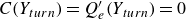 $C(Y_{turn})=Q_{e}^{\prime}(Y_{turn})=0$
; that is,
$C(Y_{turn})=Q_{e}^{\prime}(Y_{turn})=0$
; that is,
 $Y_{turn} \in [Y_{-}, Y_{+}]$
.
$Y_{turn} \in [Y_{-}, Y_{+}]$
.
Importantly, the governing dispersive equation also forms compound-wave structures when
 $Q_{e}(Y)$
is not convex. Although rarefactions still occur, far-field states are instead linked by kink solitons or intrusions analogous to a shock, or by a DSW provided
$Q_{e}(Y)$
is not convex. Although rarefactions still occur, far-field states are instead linked by kink solitons or intrusions analogous to a shock, or by a DSW provided
 $Y_{+} \neq 0$
. Here, a DSW is a wave structure slowly modulated in amplitude and frequency connecting two far-field states with different propagation speeds at each edge: one being a linear wavepacket and the other a solitary wavepacket. The dispersive-shock fitting method (El Reference El2005) that analyses DSW properties is valid if the governing PV equation satisfies a certain set of conditions outlined in Appendix A.1.
$Y_{+} \neq 0$
. Here, a DSW is a wave structure slowly modulated in amplitude and frequency connecting two far-field states with different propagation speeds at each edge: one being a linear wavepacket and the other a solitary wavepacket. The dispersive-shock fitting method (El Reference El2005) that analyses DSW properties is valid if the governing PV equation satisfies a certain set of conditions outlined in Appendix A.1.
For solutions of the form
 $Y=Y_{\infty }+\eta e^{i(kx-\omega t)}$
,
$Y=Y_{\infty }+\eta e^{i(kx-\omega t)}$
,
 $\eta \ll \mathcal{O}(1)$
of waves propagating on a background
$\eta \ll \mathcal{O}(1)$
of waves propagating on a background
 $Y_{\infty }$
, the governing PV equation for constant
$Y_{\infty }$
, the governing PV equation for constant
 $Q(x)=Q$
has a linear dispersion relation, where
$Q(x)=Q$
has a linear dispersion relation, where
 $\mathcal{O}(\eta ^2)$
terms or higher are ignored, given by
$\mathcal{O}(\eta ^2)$
terms or higher are ignored, given by
 \begin{equation} \omega (k)=C(Y_{\infty })k-\frac {a^2\mathit{\Pi }}{4}\mathcal{G}(Y_{\infty })k^3, \end{equation}
where
 $C(Y)= ({Q}/{a}+a\mathit{\Pi } )e^{-Y/a}-a\mathit{\Pi }e^{-2Y/a}, \ \mathcal{G}(Y)=a-(a+2Y)e^{-2Y/a}$
.
$C(Y)= ({Q}/{a}+a\mathit{\Pi } )e^{-Y/a}-a\mathit{\Pi }e^{-2Y/a}, \ \mathcal{G}(Y)=a-(a+2Y)e^{-2Y/a}$
.
We denote the linear-wave-edge wavenumber as
 $k$
with dispersion relation
$k$
with dispersion relation
 $\omega (k)$
, and the conjugate wavenumber of the solitary-wave edge as
$\omega (k)$
, and the conjugate wavenumber of the solitary-wave edge as
 $\tilde {k}$
, typically defined as the inverse half-width of the solitary wave, with conjugate dispersion relation
$\tilde {k}$
, typically defined as the inverse half-width of the solitary wave, with conjugate dispersion relation
 $\tilde {\omega }(\tilde {k})=-i\omega (ik)$
. In this problem the far-field states are given by
$\tilde {\omega }(\tilde {k})=-i\omega (ik)$
. In this problem the far-field states are given by
 $Y_{I} \neq 0$
(the intrusion width) and either
$Y_{I} \neq 0$
(the intrusion width) and either
 $\ Y_{-}, \ Y_{+} \neq 0$
according to the sign of the PV
$\ Y_{-}, \ Y_{+} \neq 0$
according to the sign of the PV
 $\mathit{\Pi }$
. We can find the wavenumber or conjugate wavenumber by solving the ODEs derived by El (Reference El2005) to obtain JJ20 for general constant
$\mathit{\Pi }$
. We can find the wavenumber or conjugate wavenumber by solving the ODEs derived by El (Reference El2005) to obtain JJ20 for general constant
 $Q(x)=Q$
 \begin{align} {\boldsymbol\Pi } & = -1: \notag \\ k_{-}^2 & = \frac {-8}{3a^2\mathcal{G}(Y_{-})^{2/3}}\int _{Y_{I}}^{Y_{-}}\frac {C^{\prime}(Y)}{\mathcal{G}(Y)^{1/3}} \ {\textrm{d}}Y, \quad \tilde {k}_{I}^2=\frac {8}{3a^2\mathcal{G}(Y_{I})^{2/3}}\int _{Y_{-}}^{Y_{I}}\frac {C^{\prime}(Y)}{\mathcal{G}(Y)^{1/3}} \ {\textrm{d}}Y, \end{align}
 \begin{align} {\boldsymbol\Pi } & = +1: \notag \\ k_{+}^2 & = \frac {8}{3a^2\mathcal{G}(Y_{+})^{2/3}}\int _{Y_{I}}^{Y_{+}}\frac {C^{\prime}(Y)}{\mathcal{G}(Y)^{1/3}} \ {\textrm{d}}Y, \quad \tilde {k}_{I}^2=\frac {-8}{3a^2\mathcal{G}(Y_{I})^{2/3}}\int _{Y_{+}}^{Y_{I}}\frac {C^{\prime}(Y)}{\mathcal{G}(Y)^{1/3}} \ {\textrm{d}}Y, \\[6pt] \nonumber \end{align}
where
 $k_{-}$
is the wavenumber of the linear-waveedge (
$k_{-}$
is the wavenumber of the linear-waveedge (
 $\tilde {k}_{I}=0$
here), and
$\tilde {k}_{I}=0$
here), and
 $\tilde {k}_{I}$
is the conjugate wavenumber of the solitary-waveedge (
$\tilde {k}_{I}$
is the conjugate wavenumber of the solitary-waveedge (
 $k_{-}=0$
here).
$k_{-}=0$
here).
Thus, the DSW forms a compound-wave structure with the upstream steady current (
 $Y_{-}, \mathit{\Pi }=-1$
), where the DSW travels leftward from the linear-wave edge at
$Y_{-}, \mathit{\Pi }=-1$
), where the DSW travels leftward from the linear-wave edge at
 $Y_{-}$
to the solitary-wave edge at
$Y_{-}$
to the solitary-wave edge at
 $Y_{I}$
where it connects to an intrusion on the left; or with the downstream steady current (
$Y_{I}$
where it connects to an intrusion on the left; or with the downstream steady current (
 $Y_{+}, \mathit{\Pi }=+1$
), where the DSW travels rightward from the linear-wave edge at
$Y_{+}, \mathit{\Pi }=+1$
), where the DSW travels rightward from the linear-wave edge at
 $Y_{+}$
to the solitary wave-edge at
$Y_{+}$
to the solitary wave-edge at
 $Y_{I}$
where it connects to an intrusion on the right. The propagation speeds of the solitary- and linear-wave edges are
$Y_{I}$
where it connects to an intrusion on the right. The propagation speeds of the solitary- and linear-wave edges are
 \begin{equation} s_{\pm }=\frac {\partial \omega }{\partial k}(Y_{\pm }, k_{\pm }), \quad \tilde {s}_{I}=\tilde {\omega }(Y_{I}, \tilde {k}_{I})/\tilde {k_{I}}, \end{equation}
computing the speeds and the amplitude of the solitary wave at
 $Y_{I}$
, denoted by
$Y_{I}$
, denoted by
 $Y_{s}$
, as well as the wavelength of the linear wave at
$Y_{s}$
, as well as the wavelength of the linear wave at
 $Y_{\pm }$
. Sections 4.3 and 4.4 give examples of DSWs.
$Y_{\pm }$
. Sections 4.3 and 4.4 give examples of DSWs.
4.3.
The structure of the PV front: the
$\mathit{\Pi }=+1$
positive PV case

4.3.1. Upstream of the source,
$x\lt -W$
: Q = 0,
$\mathit{\Pi }=+1$


The upstream flow of
 $\mathit{\Pi }=+1$
is well captured by the hydraulic theory of JSM17. The flow is led by a shock and terminates at the edge of the source outflow and control point
$\mathit{\Pi }=+1$
is well captured by the hydraulic theory of JSM17. The flow is led by a shock and terminates at the edge of the source outflow and control point
 $x=-W$
, so
$x=-W$
, so
 $Y_{-} \equiv 0, \ x \leqslant -W$
for all
$Y_{-} \equiv 0, \ x \leqslant -W$
for all
 $a$
. The unsteady dispersive equation is ignored as it gives a poor representation of the upstream flow, predicting negative values to indicate wave overturning as discussed in § 3.1.2.
$a$
. The unsteady dispersive equation is ignored as it gives a poor representation of the upstream flow, predicting negative values to indicate wave overturning as discussed in § 3.1.2.
4.3.2. Downstream of the source,
$x\gt W$
: Q = 1,
$\mathit{\Pi }=+1$


Downstream the source outflow,
 $x \gt W$
, the flux function
$x \gt W$
, the flux function
 $Q_{e}(Y)$
is always non-convex in the solution if
$Q_{e}(Y)$
is always non-convex in the solution if
 \begin{equation} Y_{turn}=a\ln \left (\frac {2a^2}{a^2+1}\right ) \geqslant 0. \end{equation}
For
 $a \lt 1$
a rarefaction joins these states and thus we denote
$a \lt 1$
a rarefaction joins these states and thus we denote
 $a_{r, \ +1}=1$
as the value of
$a_{r, \ +1}=1$
as the value of
 $a$
when a rarefaction just forms. Equation (4.6) is satisfied provided
$a$
when a rarefaction just forms. Equation (4.6) is satisfied provided
 $a \geqslant 1$
, where an intrusion connects the downstream current
$a \geqslant 1$
, where an intrusion connects the downstream current
 $Y_{+}$
to the coast with a finite slope and current width
$Y_{+}$
to the coast with a finite slope and current width
 $Y_{I}$
determined by (2.18) and (2.20). A rarefaction, if it occurs, propagates according to the equation
$Y_{I}$
determined by (2.18) and (2.20). A rarefaction, if it occurs, propagates according to the equation
 \begin{align} &\frac {x}{t}=C(Y)=\frac {1}{a}\left (1+a^2\right )e^{-Y/a}-ae^{-2Y/a} , \quad C(Y_{+})\lt C(Y) \lt C(Y=Y_{join}) \equiv \frac {1}{a}, \end{align}
where
 $Y_{join}$
refers to
$Y_{join}$
refers to
 $Y=0$
if a rarefaction fully joins to the coast, or
$Y=0$
if a rarefaction fully joins to the coast, or
 $Y_{I}$
if a rarefaction joins to an intrusion instead.
$Y_{I}$
if a rarefaction joins to an intrusion instead.
(a) Dispersive solution for
 $\mathit{\Pi }=+1, \ a=1.3$
and widths
$\mathit{\Pi }=+1, \ a=1.3$
and widths
 $W=3, \ 10, \ 20$
(overlaid as blue; dashed, dash-dotted, dotted respectively), compared directly with the point source contour-dynamics simulation (black) at time
$W=3, \ 10, \ 20$
(overlaid as blue; dashed, dash-dotted, dotted respectively), compared directly with the point source contour-dynamics simulation (black) at time
 $t=1000$
, focusing on the
$t=1000$
, focusing on the
 $Y_{+}$
region and upstream. (b) Similar to top but for width
$Y_{+}$
region and upstream. (b) Similar to top but for width
 $W=10$
and
$W=10$
and
 $a=0.8, \ 1.0, \ 1.3, \ 1.75$
(yellow-dashed, yellow, black-dashed, black, respectively) run until
$a=0.8, \ 1.0, \ 1.3, \ 1.75$
(yellow-dashed, yellow, black-dashed, black, respectively) run until
 $t=4000$
. The dotted lines in both figures correspond to the theoretical predictions of the structure’s locations.
$t=4000$
. The dotted lines in both figures correspond to the theoretical predictions of the structure’s locations.

We also require for any soliton or intrusion that the stationary points of
 $Y_{\xi }$
in (2.15) must be local minima (representing a stable equilibrium of the far-field states), i.e.
$Y_{\xi }$
in (2.15) must be local minima (representing a stable equilibrium of the far-field states), i.e.
 \begin{align} \nu ^{\prime\prime}(Y_{I}) \gt 0 \implies |s_{I}|\gt |C(Y_{I})|, \end{align}
consequently, an intrusion always overtakes a rarefaction and joins the far-field state to the coast. This forms a constant-width current region that is referred to herein as a ‘shelf’. We can calculate the values for which the shelf is wider or narrower than the immediate downstream current
 $Y_{+}$
by determining when
$Y_{+}$
by determining when
 \begin{equation} Y_{I} = (Y_{+})_{hyd}. \end{equation}
We denote the value of
 $a$
for which (4.9) is satisfied by
$a$
for which (4.9) is satisfied by
 $a_{I, \ +1}$
. Then for all
$a_{I, \ +1}$
. Then for all
 $a \gt a_{I, \ +1}$
, the intrusion shelf always remains wider than the constant-width downstream current
$a \gt a_{I, \ +1}$
, the intrusion shelf always remains wider than the constant-width downstream current
 $Y_{+}$
, leading to DSW formation. A shelf cannot form if the speed of the leading soliton edge of the DSW
$Y_{+}$
, leading to DSW formation. A shelf cannot form if the speed of the leading soliton edge of the DSW
 $\tilde {s}_{I}$
matches the speed of the intrusion
$\tilde {s}_{I}$
matches the speed of the intrusion
 $s_{I}$
, which occurs when
$s_{I}$
, which occurs when
 \begin{equation} \tilde {s}_{I} = s_{I}. \end{equation}
We denote the value of
 $a$
for which (4.10) holds by
$a$
for which (4.10) holds by
 $a_{crit, \ +1}$
. For
$a_{crit, \ +1}$
. For
 $a \gt a_{crit, \ +1}$
, a wall-bounded wavetrain joins the far-field current to the coast as illustrated in § 4.5. The values of
$a \gt a_{crit, \ +1}$
, a wall-bounded wavetrain joins the far-field current to the coast as illustrated in § 4.5. The values of
 $a_{r, \ +1}$
,
$a_{r, \ +1}$
,
 $a_{I, \ +1}$
and
$a_{I, \ +1}$
and
 $a_{crit, \ +1}$
are given in table 2.
$a_{crit, \ +1}$
are given in table 2.
The values of
 $a$
where different behaviours of the upstream PV front form for
$a$
where different behaviours of the upstream PV front form for
 $\mathit{\Pi }=+1$
.
$\mathit{\Pi }=+1$
.

The type of structures that form also vary with the outflow width
 $W$
in the dispersive equation. However, as noted in § 3.3, this is an artefact of the dispersive equation which does not reflect the behaviour of the full problem. Although changing the source width
$W$
in the dispersive equation. However, as noted in § 3.3, this is an artefact of the dispersive equation which does not reflect the behaviour of the full problem. Although changing the source width
 $W$
does not affect
$W$
does not affect
 $Y_{+}$
in the full QG equations, it introduces more waves to the system due to dispersion. Herein, irrespective of
$Y_{+}$
in the full QG equations, it introduces more waves to the system due to dispersion. Herein, irrespective of
 $W$
, we only use hydraulic solutions
$W$
, we only use hydraulic solutions
 $(Y_{+})_{hyd}$
to estimate the actual downstream current width.
$(Y_{+})_{hyd}$
to estimate the actual downstream current width.
Figure 8(a) shows the numerical differences in the downstream behaviour by comparing the point source
 $W=0$
contour dynamics with the dispersive dynamics at widths
$W=0$
contour dynamics with the dispersive dynamics at widths
 $W=3, \ 10, \ 20$
for
$W=3, \ 10, \ 20$
for
 $a=1.3$
. In the
$a=1.3$
. In the
 $W=3$
case, the dispersive dynamics captures the waves propagating upstream of the source, but the
$W=3$
case, the dispersive dynamics captures the waves propagating upstream of the source, but the
 $W=10, \ 20$
outflows capture
$W=10, \ 20$
outflows capture
 $Y_{+}$
better and so the simulations below are restricted, unless noted, to the width
$Y_{+}$
better and so the simulations below are restricted, unless noted, to the width
 $W=10$
for
$W=10$
for
 $\mathit{\Pi }=+1$
. This width closely matches to the point source prediction of
$\mathit{\Pi }=+1$
. This width closely matches to the point source prediction of
 $Y_{+}$
, yet is not so large that dispersive waves interfere with the solution (as with
$Y_{+}$
, yet is not so large that dispersive waves interfere with the solution (as with
 $W=20$
). The contour dynamics also matches reasonably well to the predicted intrusion location at
$W=20$
). The contour dynamics also matches reasonably well to the predicted intrusion location at
 $t=500$
from travelling-wave theory. This is shown further in figure 8(b) where the predicted intrusions, rarefactions
$t=500$
from travelling-wave theory. This is shown further in figure 8(b) where the predicted intrusions, rarefactions
 $C(Y=0)$
and long-wave propagation
$C(Y=0)$
and long-wave propagation
 $C(Y=Y_{+})$
locations align well at
$C(Y=Y_{+})$
locations align well at
 $t=4000$
for a range of values of
$t=4000$
for a range of values of
 $a$
.
$a$
.
We verify El’s technique for
 $a=1.75\gt a_{I, \ +1}$
where DSWs can form. Figure 9 shows a DSW propagating to the right downstream at
$a=1.75\gt a_{I, \ +1}$
where DSWs can form. Figure 9 shows a DSW propagating to the right downstream at
 $t=10000$
(where the DSW is fully developed), where there is a rightwards solitary-wave leading edge and a linear-wave trailing edge, terminating by an intrusion (a kink-DSW structure). As the DSW develops, the outflow sets the downstream frontal width to
$t=10000$
(where the DSW is fully developed), where there is a rightwards solitary-wave leading edge and a linear-wave trailing edge, terminating by an intrusion (a kink-DSW structure). As the DSW develops, the outflow sets the downstream frontal width to
 $(Y_{+})_{hyd}$
almost immediately (compared with DSW formation) and propagates rightwards as an almost pure wavetrain (see figure 19(b) at time
$(Y_{+})_{hyd}$
almost immediately (compared with DSW formation) and propagates rightwards as an almost pure wavetrain (see figure 19(b) at time
 $t=200$
). This leading wave amplitude continues to grow until it is limited by the width of the now fully formed intrusion (see figure 19(b) at time
$t=200$
). This leading wave amplitude continues to grow until it is limited by the width of the now fully formed intrusion (see figure 19(b) at time
 $t=500$
), determining the height and speed of the soliton edge. The soliton edge falls behind the intrusion, which travels faster to form a constant-width shelf, and thus forms the DSW. The intrusion has corresponding width and speed
$t=500$
), determining the height and speed of the soliton edge. The soliton edge falls behind the intrusion, which travels faster to form a constant-width shelf, and thus forms the DSW. The intrusion has corresponding width and speed
 $Y_{I}, s_{I}$
that is well matched with the theoretical travelling-wave theory; similarly, the theoretical dispersive-shock fitting matches well with the trailing, leading positions and the soliton width at the leading edge
$Y_{I}, s_{I}$
that is well matched with the theoretical travelling-wave theory; similarly, the theoretical dispersive-shock fitting matches well with the trailing, leading positions and the soliton width at the leading edge
 $s_{-}t$
,
$s_{-}t$
,
 $\tilde {s}_{I}t$
,
$\tilde {s}_{I}t$
,
 $Y_{s}$
for
$Y_{s}$
for
 $t=10\,000$
. We deduce the linear-wave wavelength of the DSW by calculating the distance
$t=10\,000$
. We deduce the linear-wave wavelength of the DSW by calculating the distance
 $2\pi /k_{-}$
, given by the two dotted lines along the trailing edge shown in the figure, again showing good agreement.
$2\pi /k_{-}$
, given by the two dotted lines along the trailing edge shown in the figure, again showing good agreement.
In summary,
-
(i) If
$0 \leqslant a \leqslant a_{r, \ +1}$
:
$Y_{+}$
joins the coast through a rarefaction (see figure 8
b, labelled yellow). -
(ii) If
$a_{r, \ +1} \lt a \leqslant a_{I, \ +1}$
: the PV front from
$Y_{+}$
joins the coast through an intrusion of width
$Y_{I}$
, and a compound-wave intrusion–rarefaction joins to the downstream current
$Y_{+}$
. Here,
$0 \lt Y_{I} \lt Y_{+}$
(see figure 8
b, labelled black-dashed). -
(iii) If
$a_{I, \ +1} \lt a \leqslant a_{crit, \ +1}$
: an intrusion joins the coast with current width
$Y_{I}$
, and a compound-wave intrusion-DSW joins to
$Y_{+}$
for all widths
$W$
. Here,
$0 \lt Y_{+} \lt Y_{I}$
(see figure 9). -
(iv) If
$a \gt a_{crit, \ +1}$
: a shelf no longer forms, and the upstream current becomes a wall-bounded wavetrain (see figure 15
b).


The numerical solution to the governing dispersive equation with
 $\mathit{\Pi }=+1$
and
$\mathit{\Pi }=+1$
and
 $a=1.75$
, run until
$a=1.75$
, run until
 $t=10000$
, showing a DSW propagating upstream. The source outflow centred at
$t=10000$
, showing a DSW propagating upstream. The source outflow centred at
 $x=0$
is
$x=0$
is
 $Q(x) \equiv Q_{4}(x)$
with width
$Q(x) \equiv Q_{4}(x)$
with width
 $W=10$
. The dotted lines represent the predictions of the dispersive analysis using El’s technique and travelling-wave solutions.
$W=10$
. The dotted lines represent the predictions of the dispersive analysis using El’s technique and travelling-wave solutions.

The parameter regimes for these cases are indicated in figure 10 showing the current widths and speeds
 $Y, \ s$
of any structures that form according to
$Y, \ s$
of any structures that form according to
 $a$
in the
$a$
in the
 $W=10$
dispersive integrations. In all regions
$W=10$
dispersive integrations. In all regions
 $a \lt a_{crit, \ +1}$
there is good agreement between the theoretical predictions and the numerical simulations for the speeds of the intrusions, solitons and rarefactions (panel b). As
$a \lt a_{crit, \ +1}$
there is good agreement between the theoretical predictions and the numerical simulations for the speeds of the intrusions, solitons and rarefactions (panel b). As
 $a \to 0$
the downstream speed of the rarefaction tends to infinity and numerical simulations become more challenging. If the intrusion speed
$a \to 0$
the downstream speed of the rarefaction tends to infinity and numerical simulations become more challenging. If the intrusion speed
 $s_{I}$
matches the soliton edge speed
$s_{I}$
matches the soliton edge speed
 $\tilde {s}_{I}$
, the soliton edge
$\tilde {s}_{I}$
, the soliton edge
 $Y_{s}$
reaches the coast leading to a change in behaviour. For
$Y_{s}$
reaches the coast leading to a change in behaviour. For
 $a \geqslant a_{crit, \ +1}$
, the flow forms a wall-bounded wavetrain connecting the far field to the coast. The width of the new wall-bounded wavetrain (shown in dashed lines in figure 10) differs significantly from that of the intrusion and is discussed in § 4.5.
$a \geqslant a_{crit, \ +1}$
, the flow forms a wall-bounded wavetrain connecting the far field to the coast. The width of the new wall-bounded wavetrain (shown in dashed lines in figure 10) differs significantly from that of the intrusion and is discussed in § 4.5.
Downstream behaviour of the dispersive equation for
 $\mathit{\Pi }=+1$
. The numbers i)–iv) describe regions of
$\mathit{\Pi }=+1$
. The numbers i)–iv) describe regions of
 $a$
where different behaviours of the front occur. (a) The theoretical and numerical (
$a$
where different behaviours of the front occur. (a) The theoretical and numerical (
 $W=10$
) widths of
$W=10$
) widths of
 $Y_{I}$
(black, plotted diamond),
$Y_{I}$
(black, plotted diamond),
 $Y_{+}$
(orange, plotted square) and
$Y_{+}$
(orange, plotted square) and
 $Y_{s}$
(blue, plotted circle) if a DSW forms. (b) The respective speeds for
$Y_{s}$
(blue, plotted circle) if a DSW forms. (b) The respective speeds for
 $s_{r}$
(black dash-dotted, plotted stars),
$s_{r}$
(black dash-dotted, plotted stars),
 $s_{I}$
(red lined, plotted diamond),
$s_{I}$
(red lined, plotted diamond),
 $\tilde {s}_{I}$
(blue, plotted circle). All simulations are run for at least
$\tilde {s}_{I}$
(blue, plotted circle). All simulations are run for at least
 $t \geqslant 1000$
so
$t \geqslant 1000$
so
 $Y_{+}$
becomes steady.
$Y_{+}$
becomes steady.

4.4. The structure of the PV front: the
$\mathit{\Pi }=-1$
negative PV case

The structures in the negative PV case are similar to those of the positive PV case but now the current widths
 $Y_{\pm }$
also depend on the source width
$Y_{\pm }$
also depend on the source width
 $W$
.
$W$
.
4.4.1. Upstream of the source,
$x\lt -W$
:
$Q=0$
,
$\mathit{\Pi }=-1$


Upstream, where
 $Q=0, \ x\lt -W$
, since
$Q=0, \ x\lt -W$
, since
 $|C(Y=0)| \lt |C(Y=Y_{-})| \quad \forall \ Y_{-} \gt 0$
, a shock forms immediately in the hydraulic equation (JSM17). In the dispersive equation, this shock is replaced by an intrusion. Unless the intrusion is of the same width as
$|C(Y=0)| \lt |C(Y=Y_{-})| \quad \forall \ Y_{-} \gt 0$
, a shock forms immediately in the hydraulic equation (JSM17). In the dispersive equation, this shock is replaced by an intrusion. Unless the intrusion is of the same width as
 $Y_{-}$
, compound-wave structures appear, independently of whether
$Y_{-}$
, compound-wave structures appear, independently of whether
 $Q_{e}(Y)$
is convex or not. This is true even for
$Q_{e}(Y)$
is convex or not. This is true even for
 $a \leqslant 1$
when there are no steady solutions. Again the intrusion meets the coast with finite slope and current width
$a \leqslant 1$
when there are no steady solutions. Again the intrusion meets the coast with finite slope and current width
 $Y_{I}$
predicted by (2.18) and (2.20). As in (4.8) the intrusion satisfies
$Y_{I}$
predicted by (2.18) and (2.20). As in (4.8) the intrusion satisfies
 $\nu ^{\prime\prime}(Y_{I}) \gt 0$
, travelling faster than any rarefaction, so the constant-width shelf formed by the intrusion lengthens over time (in the
$\nu ^{\prime\prime}(Y_{I}) \gt 0$
, travelling faster than any rarefaction, so the constant-width shelf formed by the intrusion lengthens over time (in the
 $x$
-direction) before joining
$x$
-direction) before joining
 $Y_{1}$
through either a rarefaction, with equation
$Y_{1}$
through either a rarefaction, with equation
 \begin{align} &\frac {x}{t}=C(Y)=ae^{-2Y/a}-ae^{-Y/a}, \end{align}
if
 $Y_{I}\lt Y_{1}$
, or through a DSW if
$Y_{I}\lt Y_{1}$
, or through a DSW if
 $Y_{I}\gt Y_{1}$
. As in § 4.3.2, we can determine the values of
$Y_{I}\gt Y_{1}$
. As in § 4.3.2, we can determine the values of
 $a$
for which the shelf is as wide as the constant-width current
$a$
for which the shelf is as wide as the constant-width current
 $Y_{-}$
for long times by determining when
$Y_{-}$
for long times by determining when
 \begin{equation} Y_{I}=Y_{-}, \end{equation}
and again (4.10) determines when a shelf no longer forms. Since changing the source width leads to two different bounds of
 $Y_{-}$
, this also gives two different values of
$Y_{-}$
, this also gives two different values of
 $a$
for when these behaviours occur. These values and their corresponding notation are given in table 3. Figure 11 shows a kink-rarefaction structure for
$a$
for when these behaviours occur. These values and their corresponding notation are given in table 3. Figure 11 shows a kink-rarefaction structure for
 $a=1.3$
and an example of shelf formation in figure 11(a). The position, width and gradient of the intrusion are well predicted as is the position of the rarefaction by long-wave speed
$a=1.3$
and an example of shelf formation in figure 11(a). The position, width and gradient of the intrusion are well predicted as is the position of the rarefaction by long-wave speed
 $C(Y)$
. Figure 12 gives another example of an (upstream) DSW where its solitary edge propagates leftward. The discussion of the theoretical predictions (dotted in figure) is identical to that following figure 9 in the positive PV case, with both the predicted locations and widths agreeing well with the dispersive integrations.
$C(Y)$
. Figure 12 gives another example of an (upstream) DSW where its solitary edge propagates leftward. The discussion of the theoretical predictions (dotted in figure) is identical to that following figure 9 in the positive PV case, with both the predicted locations and widths agreeing well with the dispersive integrations.
The values of
 $a$
for the different upstream behaviours of the PV front for
$a$
for the different upstream behaviours of the PV front for
 $\mathit{\Pi }=-1$
.
$\mathit{\Pi }=-1$
.

(a) The upstream analytical predictions (in dash-dotted) of the rarefaction and intrusion locations and the numerical integrations of the
 $\mathit{\Pi }=-1, \ a=1.3$
dispersive equation at
$\mathit{\Pi }=-1, \ a=1.3$
dispersive equation at
 $t=10000$
,
$t=10000$
,
 $W=3$
. (b) The analytical prediction of the gradient of the intrusion, zoomed in from the top figure. Note the gradient line (dashed) is adjusted very slightly from
$W=3$
. (b) The analytical prediction of the gradient of the intrusion, zoomed in from the top figure. Note the gradient line (dashed) is adjusted very slightly from
 $s_{I}t$
, the predicted intrusion location (marked as a cross
$s_{I}t$
, the predicted intrusion location (marked as a cross
 $\times$
), for clarity of comparison.
$\times$
), for clarity of comparison.

In summary,
-
(i) If
$0 \leqslant a \leqslant a_{lower, \ -1}$
: the PV front joins the coast through an intrusion with current width
$Y_{I}$
, followed by a rarefaction that joins to the downstream current
$Y_{-}$
. Here,
$0 \lt Y_{I} \lt Y_{-}$
(see figure 11(a)). -
(ii) If
$a_{lower, \ -1} \lt a \lt a_{higher, \ -1}$
: as in case (i) above for sufficiently large
$W$
, but through a rarefaction–intrusion for sufficiently small
$W$
. -
(iii) If
$a_{higher, \ -1} \leqslant a \leqslant a_{crit, \ -1, \ min}$
: for all
$W$
, an intrusion of width
$Y_{I}$
, joins the coast followed by a DSW that joins the downstream current of width
$Y_{-}$
. Here,
$0 \lt Y_{-} \lt Y_{I}$
(see figure 12). -
(iv) If
$a_{crit, \ -1, \ min} \lt a \leqslant a_{crit, \ -1, \ max}$
: this gives the lower (when
$W=\infty$
) and upper bound (when
$W=0$
) of when a shelf can form. -
(v) If
$a \gt a_{crit, \ -1, \ max}$
: for all
$W$
, a shelf no longer forms. Instead, the downstream current terminates towards the coast via a series of modulated, periodic travelling waves, described here as a wall-bounded wavetrain (see figure 15(b)).


(a) As in figure 9 but with
 $\mathit{\Pi }=-1$
,
$\mathit{\Pi }=-1$
,
 $a=1.75$
and
$a=1.75$
and
 $W=3$
, run until
$W=3$
, run until
 $t=10000$
. (b) As in (a) but with a source outflow
$t=10000$
. (b) As in (a) but with a source outflow
 $W=100$
run until
$W=100$
run until
 $t=10000$
. We observe oscillating ‘breathers’ forming upstream inside the DSW.
$t=10000$
. We observe oscillating ‘breathers’ forming upstream inside the DSW.

As in the case
 $\mathit{\Pi }=+1$
, changing the width of the outflow produces additional waves forming a range of different phenomena that are not straightforward to quantify. For example, figure 12(b) is identical to 12(a) but a large width outflow
$\mathit{\Pi }=+1$
, changing the width of the outflow produces additional waves forming a range of different phenomena that are not straightforward to quantify. For example, figure 12(b) is identical to 12(a) but a large width outflow
 $W=100$
is used instead. Using a very large outflow generates waves arising from dispersion that interact with the DSW forming breathers, unsteady nonlinear solutions with internal oscillations, as in Chabchoub et al. (Reference Chabchoub, Mozumi, Hoffmann, Babanin, Toffoli, Steer, van den Bremer, Akhmediev, Onorato and Waseda2019). Hoefer et al. (Reference Hoefer, Mucalica and Pelinovsky2023) analyse an exact solution that generates breathers in the Korteweg–de Vries (KdV) equation. Further KdV analytical work has determined whether solitons can tunnel through or stay trapped in some form of mean-flow (e.g. a DSW) wave (van der Sande et al. Reference van der Sande, El and Hoefer2021). In this example, the waves generated by the outflow interact with the DSW producing breathers where outflow solitons tunnel through the DSW towards the shelf. These become solitons that remain along the shelf, distinct from the solitons formed by the DSW.
$W=100$
is used instead. Using a very large outflow generates waves arising from dispersion that interact with the DSW forming breathers, unsteady nonlinear solutions with internal oscillations, as in Chabchoub et al. (Reference Chabchoub, Mozumi, Hoffmann, Babanin, Toffoli, Steer, van den Bremer, Akhmediev, Onorato and Waseda2019). Hoefer et al. (Reference Hoefer, Mucalica and Pelinovsky2023) analyse an exact solution that generates breathers in the Korteweg–de Vries (KdV) equation. Further KdV analytical work has determined whether solitons can tunnel through or stay trapped in some form of mean-flow (e.g. a DSW) wave (van der Sande et al. Reference van der Sande, El and Hoefer2021). In this example, the waves generated by the outflow interact with the DSW producing breathers where outflow solitons tunnel through the DSW towards the shelf. These become solitons that remain along the shelf, distinct from the solitons formed by the DSW.
Upstream behaviour of the dispersive equation for
 $\mathit{\Pi }=-1$
. The numbers i) to v) describe the regions of
$\mathit{\Pi }=-1$
. The numbers i) to v) describe the regions of
 $a$
where different behaviours of the front occur. (a) The theoretical and numerical widths of
$a$
where different behaviours of the front occur. (a) The theoretical and numerical widths of
 $Y_{I}$
(plotted diamond),
$Y_{I}$
(plotted diamond),
 $Y_{-}$
(shaded yellow depending on
$Y_{-}$
(shaded yellow depending on
 $W$
), and
$W$
), and
 $Y_{s}$
if a DSW forms (shaded blue depending on
$Y_{s}$
if a DSW forms (shaded blue depending on
 $W$
). (b) The theoretical and numerical speeds of
$W$
). (b) The theoretical and numerical speeds of
 $s_{I}$
(plotted diamond) and
$s_{I}$
(plotted diamond) and
 $\tilde {s}_{I}$
(shaded blue depending on
$\tilde {s}_{I}$
(shaded blue depending on
 $W$
). All simulations are run for at least
$W$
). All simulations are run for at least
 $t \geqslant 1000$
so
$t \geqslant 1000$
so
 $Y_{-}$
becomes steady.
$Y_{-}$
becomes steady.

Figure 13 shows the corresponding predictions (i) to (v) describing the structural behaviours as functions of
 $a$
against the dispersive integrations. The shaded regions give the ranges of
$a$
against the dispersive integrations. The shaded regions give the ranges of
 $Y_{s}, \ Y_{-}, \tilde {s}_{I}$
depending on the value of
$Y_{s}, \ Y_{-}, \tilde {s}_{I}$
depending on the value of
 $W$
. There is generally good agreement with the theory for i) to iv) for small and large widths (set to
$W$
. There is generally good agreement with the theory for i) to iv) for small and large widths (set to
 $W=3$
and
$W=3$
and
 $W=100$
) until
$W=100$
) until
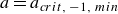 $a = a_{crit, \, -1, \ min}$
or
$a = a_{crit, \, -1, \ min}$
or
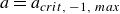 $a = a_{crit, \, -1, \ max}$
depending on the width of the source. The intrusion appears to reach a maximum width here before decreasing, out of line with the predictions (shown as an increasing dashed line in panel a). In figure 13(b), this corresponds to the DSW soliton edge speed
$a = a_{crit, \, -1, \ max}$
depending on the width of the source. The intrusion appears to reach a maximum width here before decreasing, out of line with the predictions (shown as an increasing dashed line in panel a). In figure 13(b), this corresponds to the DSW soliton edge speed
 $\tilde {s}_{I}$
matching the intrusion speed
$\tilde {s}_{I}$
matching the intrusion speed
 $s_{I}$
and a wall-bounded wavetrain forming as described in § 4.5.
$s_{I}$
and a wall-bounded wavetrain forming as described in § 4.5.
4.4.2. Downstream of the source,
$x\gt W$
:
$Q = 1$
,
$\mathit{\Pi }=-1$


The turning point width of
 $C(Y)$
is always greater than the maximum value of
$C(Y)$
is always greater than the maximum value of
 $Y_{+}$
, given by
$Y_{+}$
, given by
 $(Y_{+})_{max}$
, i.e.
$(Y_{+})_{max}$
, i.e.
 \begin{equation} Y_{turn}=a\ln \left (\frac {2a^2}{a^2-1}\right )\gt (Y_{+})_{max}=a\ln \left (\frac {a^2}{a^2-1}\right ), \end{equation}
for all
 $a$
and so any
$a$
and so any
 $Y_{+}\gt 0$
can be joined to the coast by a smooth rarefaction given by
$Y_{+}\gt 0$
can be joined to the coast by a smooth rarefaction given by
 \begin{align} &\frac {x}{t}=C(Y)=ae^{-2Y/a}+\left (\frac {1}{a}-a\right )e^{-Y/a}, \quad C(Y_{+})\lt C(Y) \lt C(Y=0) \equiv \frac {1}{a}. \end{align}
The curvature of
 $Y$
is negligible in the rarefactions and therefore so too are dispersive effects and these downstream solutions are captured well by the hydraulic equation once the dispersively determined current width is known. In the hydraulic solution
$Y$
is negligible in the rarefactions and therefore so too are dispersive effects and these downstream solutions are captured well by the hydraulic equation once the dispersively determined current width is known. In the hydraulic solution
 $(Y_{+})_{hyd}$
is fixed for all widths, and the rarefaction always begins at the control point
$(Y_{+})_{hyd}$
is fixed for all widths, and the rarefaction always begins at the control point
 $x=W$
. Figure 14 gives an example (blue circle-marked line) of a rarefaction beginning from
$x=W$
. Figure 14 gives an example (blue circle-marked line) of a rarefaction beginning from
 $x=0$
corresponding to the fluid being released from the point source
$x=0$
corresponding to the fluid being released from the point source
 $W=0$
. In the dispersive solution
$W=0$
. In the dispersive solution
 $Y_{+}$
is no longer fixed at the control point: for
$Y_{+}$
is no longer fixed at the control point: for
 $W=0$
it is determined by solving (3.20), (3.22), (3.23) giving a constant-width current whose leading edge propagates at its long-wave hydraulic speed
$W=0$
it is determined by solving (3.20), (3.22), (3.23) giving a constant-width current whose leading edge propagates at its long-wave hydraulic speed
 $C(Y_+)$
, before joining the coast through a rarefaction. This is shown in figure 14 for
$C(Y_+)$
, before joining the coast through a rarefaction. This is shown in figure 14 for
 $a=1.3$
at
$a=1.3$
at
 $t=10\,000$
with the downstream values of
$t=10\,000$
with the downstream values of
 $Y_{+}$
dependent on the width of the outflow. The locations of the rarefactions, shown by dotted lines in the figure, are well predicted analytically using the predicted steady widths
$Y_{+}$
dependent on the width of the outflow. The locations of the rarefactions, shown by dotted lines in the figure, are well predicted analytically using the predicted steady widths
 $Y_{+}$
(with
$Y_{+}$
(with
 $Y_{+}|_{hyd}$
given by (3.12). When
$Y_{+}|_{hyd}$
given by (3.12). When
 $W=100$
the solution has yet to fully settle, and the constant-width current is just emerging. The dispersive rarefaction can thus be viewed as a hydraulic rarefaction truncated at width
$W=100$
the solution has yet to fully settle, and the constant-width current is just emerging. The dispersive rarefaction can thus be viewed as a hydraulic rarefaction truncated at width
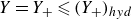 $Y=Y_{+}\leqslant (Y_{+})_{hyd}$
.
$Y=Y_{+}\leqslant (Y_{+})_{hyd}$
.
Dispersive integrations of downstream rarefactions for
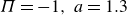 $\mathit{\Pi }=-1, \ a=1.3$
at
$\mathit{\Pi }=-1, \ a=1.3$
at
 $t=10000$
, for widths
$t=10000$
, for widths
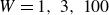 $W=1, \ 3, \ 100$
(in black, labelled bottom, middle and top, respectively). The blue, circle-marked line gives the
$W=1, \ 3, \ 100$
(in black, labelled bottom, middle and top, respectively). The blue, circle-marked line gives the
 $W=0$
hydraulic rarefaction (4.14). For each
$W=0$
hydraulic rarefaction (4.14). For each
 $W$
the predicted value of
$W$
the predicted value of
 $Y_{+}$
is shown dotted and the numerically determined solutions is dot-dashed. The predicted locations (vertical, dotted) on the leading edge of the hydraulic rarefactions are the long-wave speeds for each current width
$Y_{+}$
is shown dotted and the numerically determined solutions is dot-dashed. The predicted locations (vertical, dotted) on the leading edge of the hydraulic rarefactions are the long-wave speeds for each current width
 $Y_{+}$
.
$Y_{+}$
.

4.5. The appearance of wall-bounded wavetrains
At a larger
 $a$
(
$a$
(
 $a\gt a_{crit, \ +1}$
for
$a\gt a_{crit, \ +1}$
for
 $\mathit{\Pi }=+1$
or
$\mathit{\Pi }=+1$
or
 $a\gt a_{crit, \ -1, \ max}$
for
$a\gt a_{crit, \ -1, \ max}$
for
 $\mathit{\Pi }=-1$
), the solitary wave leading the DSW becomes wall bounded (or coast-bounded), and propagates faster. The intrusion is replaced by a wavetrain of these faster, wall-bounded solitary waves, and the DSW truncates to the width of the wavetrain, forming a partial DSW. Hoefer et al. (Reference Hoefer, Ablowitz and Engels2008) deduce the widths of wall-bounded wavetrains for the nonlinear Schrödinge piston problem using Riemann invariants. Congy et al. (Reference Congy, El, Hoefer and Shearer2021) categorise this as part of a ‘DSW implosion’ with multiple behaviours, including the formation of a partial DSW, in the Benjamin–Bona–Mahony equation. They note that a quantitative description of partial DSWs requires significant knowledge of the underlying modulated wave. This knowledge is lacking for the governing dispersive PV equation (2.13) and so it does not appear possible to determine analytically the width of the wall-bounded wavetrain in the outflow problem.
$\mathit{\Pi }=-1$
), the solitary wave leading the DSW becomes wall bounded (or coast-bounded), and propagates faster. The intrusion is replaced by a wavetrain of these faster, wall-bounded solitary waves, and the DSW truncates to the width of the wavetrain, forming a partial DSW. Hoefer et al. (Reference Hoefer, Ablowitz and Engels2008) deduce the widths of wall-bounded wavetrains for the nonlinear Schrödinge piston problem using Riemann invariants. Congy et al. (Reference Congy, El, Hoefer and Shearer2021) categorise this as part of a ‘DSW implosion’ with multiple behaviours, including the formation of a partial DSW, in the Benjamin–Bona–Mahony equation. They note that a quantitative description of partial DSWs requires significant knowledge of the underlying modulated wave. This knowledge is lacking for the governing dispersive PV equation (2.13) and so it does not appear possible to determine analytically the width of the wall-bounded wavetrain in the outflow problem.
From (2.15), a wall-bounded solitary wave of amplitude
 $Y_{I}^{\star}$
satisfies
$Y_{I}^{\star}$
satisfies
 \begin{align} &\nu (Y=0)=\nu ^{\prime}(Y=0)=0, \quad \nu (Y=Y_{I}^{\star})=0, \end{align}
and propagates with speed
 \begin{align} s_{I}^{\star}=\frac {4a(a^2+Q\mathit{\Pi })e^{-Y_{I}^{\star}/a}-a^3e^{-2Y_{I}^{\star}/a}+(2a^2+4Q\mathit{\Pi }) Y_{I}^{\star}-(3a^3+4aQ\mathit{\Pi })}{2\mathit{\Pi }{Y_{I}^{\star}}^{2}}. \end{align}
Without the complete solution for the partial DSW, one of
 $Y_{I}^{\star}$
and
$Y_{I}^{\star}$
and
 $s_{I}^{\star}$
must be determined numerically. Figure 15 shows examples of partial DSWs propagating upstream and downstream, where the shelf formed by the intrusion at smaller
$s_{I}^{\star}$
must be determined numerically. Figure 15 shows examples of partial DSWs propagating upstream and downstream, where the shelf formed by the intrusion at smaller
 $a$
has been replaced by a wall-bounded wavetrain. The width of the wavetrain for
$a$
has been replaced by a wall-bounded wavetrain. The width of the wavetrain for
 $a=3.0$
,
$a=3.0$
,
 $\mathit{\Pi }=-1$
is smaller than the intrusion for
$\mathit{\Pi }=-1$
is smaller than the intrusion for
 $a=1.75$
in figure 12, departing from the property of solutions of (2.18), (2.19) that the intrusion width increases with
$a=1.75$
in figure 12, departing from the property of solutions of (2.18), (2.19) that the intrusion width increases with
 $a$
. Using the observed, numerically determined value of
$a$
. Using the observed, numerically determined value of
 $Y_{I}^{\star}$
accurately predicts the wavetrain speed
$Y_{I}^{\star}$
accurately predicts the wavetrain speed
 $s_{I}^{\star}$
. The emergence of the wavetrain suggests that in this parameter regime solutions of the full QG equations could break into a train of eddies as appears to be happening in figure 20 below.
$s_{I}^{\star}$
. The emergence of the wavetrain suggests that in this parameter regime solutions of the full QG equations could break into a train of eddies as appears to be happening in figure 20 below.
For larger values of
 $a$
, the interface becomes more rigid, the interface deformation term
$a$
, the interface becomes more rigid, the interface deformation term
 $\psi /a^2$
in (2.3) becomes negligible and the governing equation reduces to Poisson’s equation. The dispersive PV equation governing the coastal front then includes a non-local Hilbert operator, significantly altering the flow dynamics (Clarke & Johnson Reference Clarke and Johnson1997). Johnson & McDonald (Reference Johnson and McDonald2006) find exact steady solutions in the limit
$\psi /a^2$
in (2.3) becomes negligible and the governing equation reduces to Poisson’s equation. The dispersive PV equation governing the coastal front then includes a non-local Hilbert operator, significantly altering the flow dynamics (Clarke & Johnson Reference Clarke and Johnson1997). Johnson & McDonald (Reference Johnson and McDonald2006) find exact steady solutions in the limit
 $a\to \infty$
that align with the full QG solutions, suggesting that the present asymptotic expansion requires modification at sufficiently large
$a\to \infty$
that align with the full QG solutions, suggesting that the present asymptotic expansion requires modification at sufficiently large
 $a$
.
$a$
.
Wall-bounded wavetrains for
 $W=3$
source outflows where (a)
$W=3$
source outflows where (a)
 $a=3.0$
and
$a=3.0$
and
 $\mathit{\Pi }=-1$
and (b)
$\mathit{\Pi }=-1$
and (b)
 $a=6.0$
and
$a=6.0$
and
 $\mathit{\Pi }=+1$
at time
$\mathit{\Pi }=+1$
at time
 $t=1000$
. Section 4.5 discusses predicting the wavetrain widths,
$t=1000$
. Section 4.5 discusses predicting the wavetrain widths,
 $Y_{I}^\ast$
, and speeds
$Y_{I}^\ast$
, and speeds
 $\ s_{I}^{\star}$
.
$\ s_{I}^{\star}$
.

5. The full problem
Numerical simulations of the contour dynamics (black) and the dispersive long-wave integrations (blue, dash-dotted) for negative PV outflows
 $\mathit{\Pi } = -1$
, Rossby radius
$\mathit{\Pi } = -1$
, Rossby radius
 $a=1.3$
at
$a=1.3$
at
 $t=60, \ 200, \ 500$
, with the flux function
$t=60, \ 200, \ 500$
, with the flux function
 $Q(x):=Q_{4}(x)$
for different widths: (a)
$Q(x):=Q_{4}(x)$
for different widths: (a)
 $W=1$
, (b)
$W=1$
, (b)
 $W=3$
and (c)
$W=3$
and (c)
 $W=10$
. In (a), (b) the theoretical dispersive long-wave
$W=10$
. In (a), (b) the theoretical dispersive long-wave
 $W=0$
values of the current widths
$W=0$
values of the current widths
 $Y_{-}|_{W=0}, \ Y_{+}|_{W=0}$
(dotted) are overlaid for comparison, along with the theoretical intrusion widths and locations for all figures.
$Y_{-}|_{W=0}, \ Y_{+}|_{W=0}$
(dotted) are overlaid for comparison, along with the theoretical intrusion widths and locations for all figures.

With the structure of solutions to the dispersive equation considered we can now compare the long-wave evolution solutions with CD evolutions. The full QG system (2.3), (2.4), (2.5), (2.6) is numerically solved to a high level of accuracy using contour dynamics, incorporating contour surgery following Dritschel (Reference Dritschel1988). Solving (2.3) involves the Green’s function using the modified Bessel function
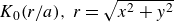 $K_{0}(r/a), \ r = \sqrt {x^2+y^2}$
following JJ20, which is further modified by introducing a source outflow along the wall. The velocity profiles associated with the
$K_{0}(r/a), \ r = \sqrt {x^2+y^2}$
following JJ20, which is further modified by introducing a source outflow along the wall. The velocity profiles associated with the
 $Q(x)=Q_{4}(x)$
source outflow are computed in Appendix A.2 while the velocity profile of the point source is given in Southwick et al. (Reference Southwick, Johnson and McDonald2017).
$Q(x)=Q_{4}(x)$
source outflow are computed in Appendix A.2 while the velocity profile of the point source is given in Southwick et al. (Reference Southwick, Johnson and McDonald2017).
As in figure 16 but with Rossby radius
 $a=1.75$
at
$a=1.75$
at
 $t=60, \ 200, \ 500$
for: (a)
$t=60, \ 200, \ 500$
for: (a)
 $W=1$
, (b)
$W=1$
, (b)
 $W=3$
and (c)
$W=3$
and (c)
 $W=10$
. Here, the width
$W=10$
. Here, the width
 $Y_{I}$
of the intrusion is wider than the width
$Y_{I}$
of the intrusion is wider than the width
 $Y_{-}$
of the flow immediately upstream outside the outflow.
$Y_{-}$
of the flow immediately upstream outside the outflow.

As in figure 16 but with
 $\mathit{\Pi }=+1, \ a=1.3$
dispersive solutions (blue, dash-dotted) overlaid with contour dynamics (black, lined) at
$\mathit{\Pi }=+1, \ a=1.3$
dispersive solutions (blue, dash-dotted) overlaid with contour dynamics (black, lined) at
 $t=60, \ 200, \ 500$
for: (a)
$t=60, \ 200, \ 500$
for: (a)
 $W=3$
, (b)
$W=3$
, (b)
 $W=10$
and (c)
$W=10$
and (c)
 $W=20$
.
$W=20$
.

Figure 16 shows for
 $a=1.3, \ \mathit{\Pi }=-1$
the improvement of the present dispersive solution over the hydraulic solution in JSM17. In JSM17, hydraulic rarefactions downstream from the outflow matched closely with the contour dynamics, and this is also captured by the dispersive integrations. There is significantly greater agreement with the current widths,
$a=1.3, \ \mathit{\Pi }=-1$
the improvement of the present dispersive solution over the hydraulic solution in JSM17. In JSM17, hydraulic rarefactions downstream from the outflow matched closely with the contour dynamics, and this is also captured by the dispersive integrations. There is significantly greater agreement with the current widths,
 $Y_{\pm }$
, adjacent to the outflow than with the hydraulic solutions
$Y_{\pm }$
, adjacent to the outflow than with the hydraulic solutions
 $(Y_{\pm })_{hyd}$
. Over long times
$(Y_{\pm })_{hyd}$
. Over long times
 $t=500$
, the solution converges to the steady solution where a constant-width current
$t=500$
, the solution converges to the steady solution where a constant-width current
 $Y_{-}$
forms just outside the source outflow upstream
$Y_{-}$
forms just outside the source outflow upstream
 $x=-W$
, with a narrower constant-width current downstream
$x=-W$
, with a narrower constant-width current downstream
 $Y_{+}$
that meets the coast through a rarefaction. This is consistent with the contour dynamics. When
$Y_{+}$
that meets the coast through a rarefaction. This is consistent with the contour dynamics. When
 $W=1$
(figure 16
a) the long-wave asymptotics produces a steep shock-like structure in the source outflow region, as predicted by § 3.2. The smaller-width sources
$W=1$
(figure 16
a) the long-wave asymptotics produces a steep shock-like structure in the source outflow region, as predicted by § 3.2. The smaller-width sources
 $W=1, \ 3$
agree remarkably well with the predicted currents
$W=1, \ 3$
agree remarkably well with the predicted currents
 $Y_{-}, Y_{+}$
of the point source contour dynamics
$Y_{-}, Y_{+}$
of the point source contour dynamics
 $W=0$
(omitted from the figure because it is graphically indistinguishable from the
$W=0$
(omitted from the figure because it is graphically indistinguishable from the
 $W=1, \ 3$
simulations), agreeing with the
$W=1, \ 3$
simulations), agreeing with the
 $W=1$
integrations to two decimal places. Only when the width is larger (
$W=1$
integrations to two decimal places. Only when the width is larger (
 $W=10$
) do the theoretical hydraulic predictions match more closely with the contour dynamics as in the steady solutions of § 3.1. The dispersive equation also accurately predicts the formation of the shelf and the location of the intrusion.
$W=10$
) do the theoretical hydraulic predictions match more closely with the contour dynamics as in the steady solutions of § 3.1. The dispersive equation also accurately predicts the formation of the shelf and the location of the intrusion.
Figure 17 shows an example where the shelf is wider than
 $Y_{-}$
, with reasonable agreement with the full problem. For larger widths (
$Y_{-}$
, with reasonable agreement with the full problem. For larger widths (
 $W=10$
), DSWs increasingly become out of phase with the full QG solutions, although the locations of their intrusions remain largely unchanged. This is because the initial contour that forms the front in the CD integrations is set up with an initial outflow width equal to (or slightly larger than)
$W=10$
), DSWs increasingly become out of phase with the full QG solutions, although the locations of their intrusions remain largely unchanged. This is because the initial contour that forms the front in the CD integrations is set up with an initial outflow width equal to (or slightly larger than)
 $W$
, improving the numerical stability, but the dispersive solutions always propagate from
$W$
, improving the numerical stability, but the dispersive solutions always propagate from
 $x=0$
. Again, the
$x=0$
. Again, the
 $W=0$
point source solutions are graphically indistinguishable from the
$W=0$
point source solutions are graphically indistinguishable from the
 $W=1, \ 3$
solutions.
$W=1, \ 3$
solutions.
There is also good agreement with the full problem in the
 $\mathit{\Pi }=+1$
case, although less strongly than for the negative PV case. The full solutions always overturn near the outflow, causing the dispersive PV front to lie below the coast at negative
$\mathit{\Pi }=+1$
case, although less strongly than for the negative PV case. The full solutions always overturn near the outflow, causing the dispersive PV front to lie below the coast at negative
 $Y$
values. This effect is most clearly seen for smaller widths in figure 18(a). The initial width of the contour is set larger than the actual source width
$Y$
values. This effect is most clearly seen for smaller widths in figure 18(a). The initial width of the contour is set larger than the actual source width
 $W$
to prevent the overturning from breaking the contour segments in the contour dynamics, but this (initially) widens the width of the upstream current before it can settle to its true value. Simulations still generally give good quantitative downstream behaviour, especially at longer times
$W$
to prevent the overturning from breaking the contour segments in the contour dynamics, but this (initially) widens the width of the upstream current before it can settle to its true value. Simulations still generally give good quantitative downstream behaviour, especially at longer times
 $t=500$
. For all widths
$t=500$
. For all widths
 $W$
, the contour dynamics chooses the current width as
$W$
, the contour dynamics chooses the current width as
 $Y_{+} \equiv (Y_{+})_{hyd}$
.
$Y_{+} \equiv (Y_{+})_{hyd}$
.
The locations of the intrusions are better predicted for the smaller-width outflows. While the intrusion speeds remain identical for all outflow widths, increasing
 $W$
alters the magnitude of overturning and increases how far the impulsively started outflow can initially propagate. The appearance of dispersive waves near the coast becomes more pronounced for the wider outflows, although there is very little dispersion (where waves are virtually constant width) immediately upstream of the source. Figure 19 compares the contour dynamics for the
$W$
alters the magnitude of overturning and increases how far the impulsively started outflow can initially propagate. The appearance of dispersive waves near the coast becomes more pronounced for the wider outflows, although there is very little dispersion (where waves are virtually constant width) immediately upstream of the source. Figure 19 compares the contour dynamics for the
 $W=10$
outflows with the dispersive integrations showing almost no difference in the case
$W=10$
outflows with the dispersive integrations showing almost no difference in the case
 $a=1.0$
. In all cases, the full solution terminates through a rarefaction or intrusion corresponding to the predictions of the dispersive equation.
$a=1.0$
. In all cases, the full solution terminates through a rarefaction or intrusion corresponding to the predictions of the dispersive equation.
Beyond
 $a=a_{crit, \ +1} \approx 1.99$
, a shelf no longer appears in the full solution; instead, a series of travelling waves that reach the coast begin to emerge. Again for larger
$a=a_{crit, \ +1} \approx 1.99$
, a shelf no longer appears in the full solution; instead, a series of travelling waves that reach the coast begin to emerge. Again for larger
 $a$
values the DSWs become out of phase, but the final positions of the intrusions for both
$a$
values the DSWs become out of phase, but the final positions of the intrusions for both
 $a=1.75, \ 2.0$
match well with the predicted dispersive locations
$a=1.75, \ 2.0$
match well with the predicted dispersive locations
 $s_{I}t$
at
$s_{I}t$
at
 $t=500$
and even at the earlier time
$t=500$
and even at the earlier time
 $t=200$
. The point source
$t=200$
. The point source
 $W=0$
contour-dynamics simulations also agree with the
$W=0$
contour-dynamics simulations also agree with the
 $W=10$
dispersive integrations, the predicted leading coastal intersection and the width
$W=10$
dispersive integrations, the predicted leading coastal intersection and the width
 $Y_{+}$
.
$Y_{+}$
.
Dispersive integrations of the
 $\mathit{\Pi }=+1$
regime (blue, dash-dotted) at different Rossby radii
$\mathit{\Pi }=+1$
regime (blue, dash-dotted) at different Rossby radii
 $a=1.0, \ 1.75, \ 2.0$
corresponding to (a), (b), (c) respectively at
$a=1.0, \ 1.75, \ 2.0$
corresponding to (a), (b), (c) respectively at
 $t=200, \ 500$
, with source outflow width
$t=200, \ 500$
, with source outflow width
 $W=10$
are compared with the corresponding contour dynamics (black, lined). Any theoretical predictions are given as dotted lines. The point source contour dynamics is also given as a comparison with the other solutions (black, dashed).
$W=10$
are compared with the corresponding contour dynamics (black, lined). Any theoretical predictions are given as dotted lines. The point source contour dynamics is also given as a comparison with the other solutions (black, dashed).

Figure 20, for
 $a=2.5$
, shows wall-bounded wavetrains beginning to form for
$a=2.5$
, shows wall-bounded wavetrains beginning to form for
 $\mathit{\Pi }= \pm 1$
in both the point source and finite-width source regimes. The simulations have been run for shorter times,
$\mathit{\Pi }= \pm 1$
in both the point source and finite-width source regimes. The simulations have been run for shorter times,
 $t=250$
, to mitigate eddy formation in the contour dynamics. For larger
$t=250$
, to mitigate eddy formation in the contour dynamics. For larger
 $a$
values, the solutions align more closely with Johnson & McDonald (Reference Johnson and McDonald2006), where the positive and negative PV solutions are simply reflections about
$a$
values, the solutions align more closely with Johnson & McDonald (Reference Johnson and McDonald2006), where the positive and negative PV solutions are simply reflections about
 $x=0$
of each other. The top figure is simulated using a lower resolution, leading to a breaking of the contour near the wall, as using a higher resolution would introduce more eddies in the PV front. The dispersive-current widths
$x=0$
of each other. The top figure is simulated using a lower resolution, leading to a breaking of the contour near the wall, as using a higher resolution would introduce more eddies in the PV front. The dispersive-current widths
 $Y_\pm$
capture the current widths in the full problem but the widths of the wavetrains in the dispersive integrations are an underestimate in both PV regimes. The full QG solutions form wall-bounded wavetrains but the leading structure is significantly larger than the preceding waves due to eddy formation caused by the competition of the velocities between the impulsively started outflow and its subsequent propagation. The difference in the overturning explains why the dispersive integrations and contour dynamics end downstream at different points in the
$Y_\pm$
capture the current widths in the full problem but the widths of the wavetrains in the dispersive integrations are an underestimate in both PV regimes. The full QG solutions form wall-bounded wavetrains but the leading structure is significantly larger than the preceding waves due to eddy formation caused by the competition of the velocities between the impulsively started outflow and its subsequent propagation. The difference in the overturning explains why the dispersive integrations and contour dynamics end downstream at different points in the
 $a=2.5, \ W=3$
simulations. While the current
$a=2.5, \ W=3$
simulations. While the current
 $Y_{+}$
reaches the coast via a rarefaction in the dispersive solution, in the full problem the current overturns and strikes the coast immediately.
$Y_{+}$
reaches the coast via a rarefaction in the dispersive solution, in the full problem the current overturns and strikes the coast immediately.
Dispersive integrations for the
 $a=2.5$
regime (blue, dash-dotted) with source outflow (a)
$a=2.5$
regime (blue, dash-dotted) with source outflow (a)
 $W=3$
,
$W=3$
,
 $\mathit{\Pi }=-1$
; and (b)
$\mathit{\Pi }=-1$
; and (b)
 $W=10$
,
$W=10$
,
 $\mathit{\Pi }=+1$
compared with the corresponding contour dynamics (black, lined) at
$\mathit{\Pi }=+1$
compared with the corresponding contour dynamics (black, lined) at
 $t=250$
. Dotted lines give the predicted current widths. The point source contour dynamics at
$t=250$
. Dotted lines give the predicted current widths. The point source contour dynamics at
 $a=2.5$
corresponding to the PV is also given as a comparison with the other solutions (black, dashed).
$a=2.5$
corresponding to the PV is also given as a comparison with the other solutions (black, dashed).

6. Discussion
JSM17 discussed the leading-order hydraulic behaviour (in the limit of large outflow width compared with current width) of coastal outflows and compared hydraulic solutions with accurate contour-dynamics simulations of the governing QG equation. Although hydraulic solutions captured much of the flow behaviour, there were significant differences in some parameter regimes. Here, we have continued the expansion to higher order, obtaining a nonlinear, dispersive, long-wave equation for the evolution of the front. At large times, the flow behaviour divides naturally into three regimes: a steady outflow region (§ 3), steady constant-width currents joined to the outflow region directly or through a truncated soliton (§ 3.1, § 3.2) and terminating unsteady propagating fronts, strongly influenced by dispersive effects (§ 4).
The widths of the steady currents are a strong function of the dispersion when the outflow PV anomaly is negative. A Rossby-wave control at the outflow, where the frontal Rossby wave is brought to rest by the flow along the front, determines what fraction of the outflow flux moves downstream. Since the position of the control depends on the geometry of the outflow, here the outflow width
 $W$
, and this means that the width of the downstream coastal current cannot be determined uniquely from global quantities like the total outflow volume flux, the PV and the density contrast. A local theory predicts the structure of the current only once the downstream flux is known. The upstream steady current width,
$W$
, and this means that the width of the downstream coastal current cannot be determined uniquely from global quantities like the total outflow volume flux, the PV and the density contrast. A local theory predicts the structure of the current only once the downstream flux is known. The upstream steady current width,
 $Y_{-}$
, is largest and the downstream steady current width,
$Y_{-}$
, is largest and the downstream steady current width,
 $Y_{+}$
, is smallest for a point source outflow. By adding dispersive terms, we identify wave overturning in the negative PV case (§ 3.3) that is absent in the hydraulic solutions.
$Y_{+}$
, is smallest for a point source outflow. By adding dispersive terms, we identify wave overturning in the negative PV case (§ 3.3) that is absent in the hydraulic solutions.
The numerical integrations of the dispersive equation capture the full QG dynamics more accurately than the hydraulic equation, obtaining new behaviour for positive PV (§ 4.3) and accurate predictions for the downstream current widths in the case of negative PV flows (§ 3.2). A rich set of behaviours, including DSW formation and compound-wave structures (rarefaction–intrusions, DSW–intrusions) observed in the QG simulations, are discussed and quantified using standard analysis techniques for nonlinear equations (§ 4.2, El (Reference El2005), JJ20) along with a novel shock-soliton solution (§ 3.2). For sufficiently large
 $a$
the dispersive equation admits travelling waves terminating in a wall-bounded wavetrain (§ 4.5) indicating a dynamical regime where coastal outflows might break into eddy trains.
$a$
the dispersive equation admits travelling waves terminating in a wall-bounded wavetrain (§ 4.5) indicating a dynamical regime where coastal outflows might break into eddy trains.
For large internal Rossby radius
 $a$
, the deformation term in (2.3) becomes negligible and the governing equation derived here no longer applies. Johnson & McDonald (Reference Johnson and McDonald2006) discuss this limit but do not present an analytical evolution theory so consideration of hydraulic and dispersive effects in near-rigid-interface flows remains an area for further study.
$a$
, the deformation term in (2.3) becomes negligible and the governing equation derived here no longer applies. Johnson & McDonald (Reference Johnson and McDonald2006) discuss this limit but do not present an analytical evolution theory so consideration of hydraulic and dispersive effects in near-rigid-interface flows remains an area for further study.
Declaration of interests
The authors report no conflict of interest.
Appendix A
A.1. Conditions for dispersive-shock fitting
In § 4.2 we describe the method to ascertain the properties of a DSW that connects two current widths in the regions of constant flux
 $Q(x)=Q$
. Here, we briefly describe, adapted from JJ20, the conditions that the governing PV equation must satisfy for this method to successfully apply:
$Q(x)=Q$
. Here, we briefly describe, adapted from JJ20, the conditions that the governing PV equation must satisfy for this method to successfully apply:
-
(i) The equation has a hydraulic (zeroth order) limit when we introduce
$X=\varepsilon x$
and
$T= \varepsilon t$
(this is done in (2.10)). -
(ii) The linear dispersion relation is real valued, given by (4.2).
-
(iii) The system possesses at least two conservation laws. The first is (2.14) for
$Q(x)=Q$
constant
$Q$
. The second conservation law for constant
$Q(x) \equiv Q$
, is from JJ20 (for
$Q=1$
). Multiplying (2.14) by
$Y$
and simplifying gives(A.1)
\begin{align} 0&=\left (\frac {Y^2}{2}\right )_{t}+\left [\frac {a^2\Pi }{4}(2Y+a)e^{-2Y/a}-(Y+a)(Q+a^2\mathit{\Pi })e^{-Y/a}\right ]_{x} \notag \\ &\quad +\left [\frac {-a^3\mathit{\Pi }}{8}(Y_{x}^2-2YY_{x})\right. \notag\\ & \quad + \left.\frac {a\mathit{\Pi }}{8}\left [4(Y^2Y_{x}^2+\frac {a}{2}YY_{x}^2)+a^2(Y_{x}^2-2YY_{xx})-4aY^2Y_{xx}\right ]e^{-2Y/a}\right ]_{x}. \end{align}
-
(iv) The equation supports periodic travelling-wave solutions parameterised by three independent variables. This is shown when writing the PV equation in potential form (2.15).
-
(v) Considering slowly modulating (changing) waves means that we are able to obtain the Whitham system, which is a set of equations involving our two conservation laws (averaged over the period of a typical travelling wave) plus the wavenumber conservation equation
$\omega _{x}+k_{t}=0$
. This system must be hyperbolic. Since the flux function
$Q_{e}(x,t)$
is non-convex, for certain intervals of
$Y$
the system may not be strictly hyperbolic and compound-wave structures form instead.


A.2. The outflow velocities of the full QG equations
The streamfunction for the zero PV part of (2.3), satisfying
 $\nabla ^2 \psi - 1/a^2 \psi = 0$
, is found by considering the velocity of the source outflow only. Southwick et al. (Reference Southwick, Johnson and McDonald2017) represent the associated horizontal velocity profiles
$\nabla ^2 \psi - 1/a^2 \psi = 0$
, is found by considering the velocity of the source outflow only. Southwick et al. (Reference Southwick, Johnson and McDonald2017) represent the associated horizontal velocity profiles
 $(u,v)$
by solving the full solution in Appendix B for a general source profile as
$(u,v)$
by solving the full solution in Appendix B for a general source profile as
 \begin{equation} \begin{pmatrix} u \\ v \end{pmatrix} = \begin{pmatrix} -\partial \psi / \partial y \\ \partial \psi / \partial x \end{pmatrix} = \frac {1}{\sqrt {2\pi }} \int ^{\infty }_{-\infty } \begin{pmatrix} \kappa \\ ik \end{pmatrix} \hat {Q}(k)e^{-\kappa y}e^{ikx} \ {\textrm{d}}k, \end{equation}
where
 $\hat {Q}(k)$
is the Fourier transform of the source
$\hat {Q}(k)$
is the Fourier transform of the source
 $Q(x)$
, and
$Q(x)$
, and
 $\kappa =(k^2+1/a^2)^{1/2}$
. For the flux function
$\kappa =(k^2+1/a^2)^{1/2}$
. For the flux function
 $Q_{4}(x)$
in (4.1), the velocity components, used in the contour dynamics to solve the full QG equation (§ 5), are given by
$Q_{4}(x)$
in (4.1), the velocity components, used in the contour dynamics to solve the full QG equation (§ 5), are given by
 \begin{align} &u=\frac {1}{2a}e^{-y/a} +\frac {1}{\pi }\int ^{\infty }_{0} \frac {64\sin (kx)\kappa e^{-\kappa y}\left (2\cos (kW)+1\right )\pi ^4}{3(81k^5W^4-180\pi ^2k^3W^2+64\pi ^4k)} \ {\textrm{d}}k, \\[-5pt] \nonumber \end{align}
 \begin{align} &v=\frac {1}{\pi }\int ^{\infty }_{0} \frac {64\cos (kx)e^{-\kappa y}\left (2\cos (kW)+1\right )\pi ^4}{3(81k^4W^4-180\pi ^2k^2W^2+64\pi ^4)} \ {\textrm{d}}k. \\[12pt] \nonumber \end{align}
The integrands in (A.3), (A.4) are bounded when
 $k \to 0$
and vanish exponentially as
$k \to 0$
and vanish exponentially as
 $k \to \infty$
for
$k \to \infty$
for
 $y\gt 0$
, giving rapidly converging integrals. On
$y\gt 0$
, giving rapidly converging integrals. On
 $y=0$
, the convergence of the integrals is only algebraic.
$y=0$
, the convergence of the integrals is only algebraic.


 Open access