




1. Introduction
The study of passive scalars evolving within wall-bounded turbulent flows has great practical importance, being relevant for the behaviour of diluted contaminants, and/or as a model for the temperature field under the assumption of low Mach number and small temperature differences (Monin & Yaglom Reference Monin and Yaglom1971; Cebeci & Bradshaw Reference Cebeci and Bradshaw1984). It is well known that measurements of concentration of passive tracers and of small temperature differences are quite difficult, and in fact available information about even basic passive scalar statistics is rather limited (Gowen & Smith Reference Gowen and Smith1967; Kader Reference Kader1981; Subramanian & Antonia Reference Subramanian and Antonia1981; Nagano & Tagawa Reference Nagano and Tagawa1988), mostly including basic mean properties and overall mass or heat transfer coefficients. The physical understanding of passive scalars in turbulent flow pertains mainly to the case  ${Pr} \approx 1$ (where the molecular Prandtl number is defined here as the ratio of the kinematic viscosity to the thermal diffusivity, ${Pr}=\nu /\alpha$), for which strong analogies exist between passive scalars and the longitudinal velocity component, as verified in a number of studies (Kim, Moin & Moser Reference Kim, Moin and Moser1987; Abe & Antonia Reference Abe and Antonia2009; Antonia, Abe & Kawamura Reference Antonia, Abe and Kawamura2009). However, many fluids, including water, engine oils, glycerol and polymer melts, have values of ${Pr}$ that can be significantly higher than unity, whereas in liquid metals and molten salts, the Prandtl number can be much less than unity. In the case of diffusions of contaminants, the Prandtl number is replaced by the Schmidt number (namely, the ratio of kinematic viscosity to mass diffusivity), whose typical values in applications are always much higher than unity (Levich Reference Levich1962). Under such circumstances, similarity between velocity and passive scalar fluctuations is substantially impaired, which makes predictions of even the basic flow statistics quite difficult. In fact, the most complete predictive theory for the behaviour of passive scalars at non-unit Prandtl number relies heavily on classical studies (Levich Reference Levich1962; Gowen & Smith Reference Gowen and Smith1967; Kader & Yaglom Reference Kader and Yaglom1972), and most predictive formulas for the heat transfer coefficients are based on semi-empirical power-law correlations (Dittus & Boelter Reference Dittus and Boelter1933; Kays, Crawford & Weigand Reference Kays, Crawford and Weigand1980). Although existing correlations may have sufficient accuracy for engineering design, their theoretical foundations are not firmly established. Furthermore, assumptions typically made in turbulence models, such as constant turbulent Prandtl number, are known to be crude approximations in the absence of reliable reference data.
Given this scenario, direct numerical simulations (DNS) are the natural candidates to establish a credible database for the physical analysis of passive scalars in wall turbulence, and for the development and validation of phenomenological prediction formulas and turbulence models. Most DNS studies of passive scalars in wall turbulence so far have been carried out for the prototype case of planar channel flow, starting with the work of Kim & Moin (Reference Kim and Moin1989), at  ${Re}_{\tau } = 180$ (here ${Re}_{\tau } = u_{\tau } h / \nu$ is the friction Reynolds number, with $u_{\tau } = (\tau _w/\rho )^{1/2}$ the friction velocity, $h$ the channel half-height, $\nu$ the fluid kinematic viscosity, $\rho$ the fluid density, and $\tau _w$ the wall shear stress), in which the forcing of the scalar field was achieved using a spatially and temporally uniform source term. Additional DNS at increasingly high Reynolds number were carried out by Kawamura, Abe & Matsuo (Reference Kawamura, Abe and Matsuo1999) and Abe, Kawamura & Matsuo (Reference Abe, Kawamura and Matsuo2004), based on enforcement of strictly constant heat flux in time (this approach is hereafter referred to as CHF), which first allowed us to appreciate scale separation effects, and to educe a reasonable value of the scalar von Kármán constant $k_{\theta } \approx 0.43$, as well as effects of Prandtl number variation. Those studies showed close similarity between the streamwise velocity and passive scalar field in the near-wall region, as after the classical Reynolds analogy. Specifically, the scalar field was found to be organized into streaks whose size scales in wall units, with a correlation coefficient between streamwise velocity fluctuations and scalar fluctuations close to unity. Computationally high Reynolds numbers ( ${Re}_{\tau } \approx 4000$, with ${Pr} \leq 1$) were reached in the study of Pirozzoli, Bernardini & Orlandi (Reference Pirozzoli, Bernardini and Orlandi2016), using spatially uniform forcing in such a way as to maintain the bulk temperature constant in time (this approach is hereafter referred to as CMT). Recent large-scale channel flow DNS with passive scalars using the CHF forcing at ${Pr}=0.71$ (as representative of air) have been carried out by Alcántara-Ávila, Hoyas & Pérez-Quiles (Reference Alcántara-Ávila, Hoyas and Pérez-Quiles2021). Prandtl number effects in plane channel flow were further addressed by Schwertfirm & Manhart (Reference Schwertfirm and Manhart2007), Alcántara-Ávila, Hoyas & Pérez-Quiles (Reference Alcántara-Ávila, Hoyas and Pérez-Quiles2018), Abe & Antonia (Reference Abe and Antonia2019), and Alcántara-Ávila & Hoyas (Reference Alcántara-Ávila and Hoyas2021), to which we will refer for comparison.
Flow in a circular pipe is clearly more practically relevant than plane channel flow in view of applications as heat exchangers, and it has been the subject of a number of experimental studies, aimed mainly at predicting the heat transfer coefficient as a function of the bulk flow Reynolds number (Kays et al. Reference Kays, Crawford and Weigand1980). High-fidelity numerical simulations including passive scalars in pipe flow so far have been quite scarce, and limited mainly to  ${Re}_{\tau } \leq 1000$ (Piller Reference Piller2005; Redjem-Saad, Ould-Rouiss & Lauriat Reference Redjem-Saad, Ould-Rouiss and Lauriat2007; Saha et al. Reference Saha, Chin, Blackburn and Ooi2011; Antoranz et al. Reference Antoranz, Gonzalo, Flores and Garcia-Villalba2015; Straub et al. Reference Straub, Forooghi, Marocco, Wetzel and Frohnapfel2019). Higher Reynolds numbers (up to ${Re}_{\tau } = 6000$) have been considered by Pirozzoli et al. (Reference Pirozzoli, Romero, Fatica, Verzicco and Orlandi2022), but at unit Prandtl numbers. Those DNS confirmed a general similarity between the axial velocity field and the passive scalar field; however, the latter was found to have additional energy at small wavenumbers, resulting in higher mixedness. Logarithmic growth of the inner-scaled bulk and mean centreline scalar values with the friction Reynolds number was found, implying an estimated scalar von Kármán constant $k_{\theta } \approx 0.459$, similar to what was found in plane channel flow (Pirozzoli et al. Reference Pirozzoli, Bernardini and Orlandi2016; Alcántara-Ávila et al. Reference Alcántara-Ávila, Hoyas and Pérez-Quiles2021). The DNS data were also used to synthesize a modified form of the classical predictive formula of Kader & Yaglom (Reference Kader and Yaglom1972). It appears that DNS data of pipe flow at both high and low Prandtl number have not been explored intensely, despite their importance.
In this paper, we thus present novel DNS data of turbulent flow in a smooth circular pipe at moderate Reynolds number  ${Re}_{\tau }=1140$, which is, however, high enough that a state of fully developed turbulence is established, with a near-logarithmic region of the mean velocity profile. A wide range of Prandtl numbers is considered, from ${Pr}=0.00625$ to ${Pr}=16$, such that some asymptotic properties for vanishing and very high Prandtl number can be inferred. This study complements our previous study about Reynolds number effects (up to ${Re}_{\tau } \approx 6000$) for passive scalars at ${Pr} = 1$ (Pirozzoli et al. Reference Pirozzoli, Romero, Fatica, Verzicco and Orlandi2022), allowing predictive extrapolations to the full range of Reynolds and Prandtl numbers. Although, as pointed out previously, the study of passive scalars is relevant in several contexts, one of the primary fields of application is heat transfer, therefore from now on, we will refer to the passive scalar field as the temperature field (denoted as $T$), and scalar fluxes will be interpreted as heat fluxes.
2. The numerical dataset
Numerical simulations of fully developed turbulent flow in a circular pipe are carried out assuming periodic boundary conditions in the axial ( $z$) and azimuthal ( $\phi$) directions, as shown in figure 1. The velocity field is controlled by two parameters, namely the bulk Reynolds number ${Re}_b = 2 R u_b / \nu$ (with $u_b$ the bulk velocity, i.e. averaged over the cross-section), and the relative pipe length $L_z/R$. The incompressible Navier–Stokes equations are supplemented with the transport equation for a passive scalar field (hence buoyancy effects are disregarded), with different values of the thermal diffusivity (hence various ${Pr}$), and with isothermal boundary conditions at the pipe wall ( $r=R$). The passive scalar equation is forced through a time-varying, spatially uniform source term (CMT approach), in the interests of achieving complete similarity with the streamwise momentum equation, with obvious exclusion of pressure. Although the total heat flux resulting from the CMT approach is not strictly constant in time, it oscillates around its mean value under statistically steady conditions. Differences of the results obtained with the CMT and CHF approaches have been pinpointed by Abe & Antonia (Reference Abe and Antonia2017) and Alcántara-Ávila et al. (Reference Alcántara-Ávila, Hoyas and Pérez-Quiles2021), which, although generally small, deserve some attention.
Definition of coordinate system for DNS of pipe flow, where  $z$,
$z$,  $r$,
$r$,  $\phi$ are the axial, radial and azimuthal directions, respectively, $R$ is the pipe radius, $L_z$ is the pipe length, and $u_b$ is the bulk velocity.

The computer code used for the DNS is the evolution of the solver developed originally by Verzicco & Orlandi (Reference Verzicco and Orlandi1996), and used for DNS of pipe flow by Orlandi & Fatica (Reference Orlandi and Fatica1997). The solver relies on second-order finite-difference discretization of the incompressible Navier–Stokes equations in cylindrical coordinates based on the classical marker-and-cell method (Harlow & Welch Reference Harlow and Welch1965), whereby pressure and passive scalars are located at the cell centres, whereas the velocity components are located at the cell faces, thus removing odd–even decoupling phenomena, and guaranteeing discrete conservation of the total kinetic energy and passive scalar variance in the inviscid limit. The Poisson equation resulting from enforcement of the divergence-free condition is solved efficiently by double trigonometric expansion in the periodic axial and azimuthal directions, and inversion of tridiagonal matrices in the radial direction (Kim & Moin Reference Kim and Moin1985). A crucial computational issue is the proper treatment of the polar singularity at the pipe axis, which we handle as suggested by Verzicco & Orlandi (Reference Verzicco and Orlandi1996), by replacing the radial velocity  $u_r$ in the governing equations with $q_r = r u_r$ (where $r$ is the radial space coordinate), which by construction vanishes at the axis. The governing equations are advanced in time by means of a hybrid third-order low-storage Runge–Kutta algorithm, whereby the diffusive terms are handled implicitly, and convective terms in the axial and radial direction explicitly. An important issue in this respect is the convective time step limitation in the azimuthal direction, due to intrinsic shrinking of the cell size towards the pipe axis. To alleviate this limitation, we use implicit treatment of the convective terms in the azimuthal direction (Akselvoll & Moin Reference Akselvoll and Moin1996; Wu & Moin Reference Wu and Moin2008), which enables marching in time with a time step similar to that in planar domain flow in practical computations. In order to minimize numerical errors associated with implicit time stepping, explicit and implicit discretizations of the azimuthal convective terms are blended linearly with the radial coordinate, in such a way that near the pipe wall, the treatment is fully explicit, and near the pipe axis, it is fully implicit. The code was adapted to run on clusters of graphic accelerators (GPUs), using a combination of CUDA Fortran and OpenACC directives, and relying on the CUFFT libraries for efficient execution of fast Fourier transforms (Ruetsch & Fatica Reference Ruetsch and Fatica2014).
From now on, inner normalization of the flow properties will be denoted with the ‘ $+$’ superscript, whereby velocities are scaled by $u_{\tau }$, wall distances ( $y=R-r$) by $\nu /u_{\tau }$, and temperatures with respect to the friction temperature,
 \begin{equation} T_{\tau} = \frac{\alpha}{u_{\tau}} \left\langle \frac {\mathrm{d} {T}}{\mathrm{d} y} \right\rangle_w. \end{equation}
In particular, the inner-scaled temperature is defined as  $\theta ^+ = (T-T_w)/T_{\tau }$, where $T$ is the local temperature, and $T_w$ is the wall temperature. Capital letters will be used to denote flow properties averaged in the homogeneous spatial directions and in time, brackets to denote the averaging operator, and lower-case letters to denote fluctuations from the mean. Instantaneous values will be denoted with a tilde, e.g. $\tilde {\theta } = \varTheta + \theta$. The bulk values of axial velocity and temperature are defined as
 \begin{equation} u_b = 2 \left.\int_0^R r \left\langle u_z \right\rangle \mathrm{d} r \right/ R^2 , \quad T_b = 2 \left.\int_0^R r \left\langle T \right\rangle \mathrm{d} r \right/ R^2 . \end{equation}
 A list of the main simulations that we have carried out is given in table 1. Eleven values of the Prandtl number are considered, from  ${Pr} = 0.00625$ to $16$. The pipe length was set to $L_z=15 R$ for all the flow cases, based on a box sensitivity study (Pirozzoli et al. Reference Pirozzoli, Romero, Fatica, Verzicco and Orlandi2022). The mesh resolution is designed based on the criteria discussed by Pirozzoli & Orlandi (Reference Pirozzoli and Orlandi2021). In particular, the collocation points are distributed in the wall-normal direction so that approximately 30 points are placed within $y^+ \leq 40$, with the first grid point at $y^+ < 0.1$, and the mesh is stretched progressively in the outer wall layer in such a way that the mesh spacing is proportional to the local Kolmogorov length scale, which there varies as $\eta ^+ \approx 0.8 \, {y^+}^{1/4}$ (Jiménez Reference Jiménez2018). Regarding the axial and azimuthal directions, finite-difference simulations of wall-bounded flows yield grid-independent results as long as $\Delta z^+ \approx 10$, $R^+\,\Delta \phi \approx 4.5$ (Pirozzoli et al. Reference Pirozzoli, Bernardini and Orlandi2016), hence we have selected the number of grid points along the homogeneous flow directions as $N_z = L_z / R \times {Re}_{\tau } / 9.8$, $N_{\phi } \sim 2 {\rm \pi}\times {Re}_{\tau } / 4.1$. A finer mesh is used for flow cases with ${Pr} > 1$, so as to satisfy restrictions on the Batchelor scalar dissipative scale, whose ratio to the Kolmogorov scale is approximately ${Pr}^{-1/2}$ (Batchelor Reference Batchelor1959; Tennekes & Lumley Reference Tennekes and Lumley1972).
Flow parameters for DNS of pipe flow at various Prandtl numbers. Here,  $N_z$, $N_r$, $N_{\phi }$ denote the numbers of grid points in the axial, radial and azimuthal directions, respectively, ${Pe}_{\tau } = {Pr} \, {Re}_{\tau }$ is the friction Péclet number, ${Nu}$ is the Nusselt number (as defined in (3.25)), and ETT is the time interval considered to collect the flow statistics, in units of the eddy-turnover time, namely $R/u_\tau$. For all simulations, $L_z = 15 R$, ${Re}_b=44\,000$ and ${Re}_{\tau }=1137.6$.

According to established practice (Hoyas & Jiménez Reference Hoyas and Jiménez2006; Ahn et al. Reference Ahn, Lee, Lee, Kang and Sung2015; Lee & Moser Reference Lee and Moser2015), the time intervals used to collect the flow statistics are reported as a fraction of the eddy-turnover time ( $R/u_{\tau }$). The sampling errors for some key properties discussed in this paper have been estimated using the method of Russo & Luchini (Reference Russo and Luchini2017), based on extension of the classical batch means approach. We have found that the sampling error is generally quite limited, being larger in the largest DNS, which are, however, carried out over a shorter time interval. In particular, in the ${Pr}=16$ flow case, the expected sampling error in Nusselt number, centreline temperature and peak temperature variance is approximately $0.5\,\%$. In order to quantify uncertainties associated with numerical discretization, additional simulations have been carried out by doubling the numbers of grid points in the azimuthal, radial and axial directions. The results show that the uncertainty due to numerical discretization and limited pipe length is approximately $0.2\,\%$ for the Nusselt number, $0.4\,\%$ for the pipe centreline temperature, and $0.7\,\%$ for the peak temperature variance.
3. Results
3.1. General organization of the temperature field
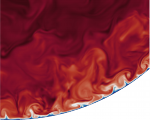
Qualitative information about the organization of the flow field is provided by instantaneous perspective views of the axial velocity and temperature fields, which we show in figures 2–4. As is well known, the flow near the pipe wall is dominated by streaks of alternating high- and low-speed fluid, which are the hallmark of wall-bounded turbulence (figures 2a, 3a, 4a); see Kline et al. (Reference Kline, Reynolds, Schraub and Runstadler1967). The temperature field at unit Prandtl number (figures 2d, 3d, 4d) exhibits a similar organization, which is not surprising on account of close formal similarity of passive scalar and axial momentum equations at  ${Pr}=1$, and close association of the two quantities was indeed pointed out in many previous studies (e.g. Abe & Antonia Reference Abe and Antonia2009; Pirozzoli et al. Reference Pirozzoli, Bernardini and Orlandi2016; Alcántara-Ávila et al. Reference Alcántara-Ávila, Hoyas and Pérez-Quiles2018). Zooming closer (see figure 4), one will nevertheless detect differences between the two fields, in that temperature tends to form sharper fronts, whereas the axial velocity field tends to be more blurred. As noted by Pirozzoli et al. (Reference Pirozzoli, Bernardini and Orlandi2016), this is due to the fact that the axial velocity is not simply advected passively, but rather it can react to the formation of fronts through feedback pressure. This reflects into shallower spectral ranges than Kolmogorov's $k^{-5/3}$ (Pirozzoli et al. Reference Pirozzoli, Romero, Fatica, Verzicco and Orlandi2022). Thermal streaks persist at ${Pr} > 1$ (figures 2e, f, 3e, f, 4e, f), and seem to retain a similar organization as in the case of unit Prandtl number. However, they tend to vanish at low Prandtl number (figures 2b,c, 3b,c, 4b,c), and are totally suppressed at ${Pr}=0.00625$, as a result of scalar diffusivity overwhelming turbulent agitation. The flow in the cross-stream planes (figures 3 and 4) is characterized by sweeps of high-speed fluid from the pipe core and ejections of low-speed fluid from the wall. Ejections and sweep have a clearly multi-scale nature, as some of them are confined to the buffer layer, whereas others manage to protrude up to the pipe centreline. At very low Prandtl number (figures 2b, 3b, 4b), turbulence is barely capable of perturbing the otherwise purely diffusive behaviour of the temperature field. The presence of details on a finer and finer scale is evident at increasing ${Pr}$, on account of the previously noted reduction of the Batchelor scale. Increase of the Prandtl number also yields progressive equalization of the temperature field over the cross-section. As a result, the large-scale eddies become weaker, and thermal agitation becomes confined mainly to the wall vicinity, within a layer whose thickness is proportional to the conductive sublayer thickness, which will be discussed extensively later.
(a) Instantaneous axial velocity contours, and temperature contours for (b)  ${Pr}=0.00625$, (c) ${Pr}=0.25$, (d) ${Pr}=1$, (e) ${Pr}=4$, and ( f) ${Pr}=16$, each normalized by the mean value at the pipe axis. The near-wall contours are taken at distance $y^+=15$.

(a) Instantaneous axial velocity contours, and temperature contours for (b)  ${Pr}=0.00625$, (c) ${Pr}=0.25$, (d) ${Pr}=1$, (e) ${Pr}=4$, and ( f) ${Pr}=16$, in a cross-sectional plane, each normalized by the mean value at the pipe axis.

(a) Instantaneous axial velocity contours, and temperature contours for (b)  ${Pr}=0.00625$, (c) ${Pr}=0.25$, (d) ${Pr}=1$, (e) ${Pr}=4$, and ( f) ${Pr}=16$, in a subregion of the pipe cross-section, each normalized by the mean value at the pipe axis. A segment with length of 100 wall units is reported for reference.

The above scenario is substantiated by the spectral maps of  $u_z$ and $\theta$, which are depicted in figure 5. The axial velocity spectra (figure 5a) clearly bring out a two-scale organization, with a near-wall peak associated with the wall regeneration cycle (Jiménez & Pinelli Reference Jiménez and Pinelli1999), and an outer peak associated with outer-layer large-scale motions (Hutchins & Marusic Reference Hutchins and Marusic2007). The latter peak is found to be centred around $y/R \approx 0.22$, and to correspond to eddies with typical wavelength $\lambda _{\phi } \approx 1.25 R$. Notably, very similar organization is found in the temperature field at unit Prandtl number (figure 5d), the main difference being a less distinct energy peak at large wavelengths. Both the axial velocity and the temperature field exhibit a prominent spectral ridge corresponding to modes with typical azimuthal length scale $\lambda _{\phi } \sim y$, extending over more than one decade, which can be interpreted as the footprint of a hierarchy of wall-attached eddies after Townsend's hypothesis (Townsend Reference Townsend1976). The spectral maps are, however, quite different at non-unit Prandtl number. At very low Prandtl number (figure 5b), all the small scales of thermal motion are filtered out by the large thermal diffusivity, and hints of organization are found only at the largest scales. The typical azimuthal length scale of these eddies appears to be $\lambda _{\phi } = {\rm \pi}R$, hence only two pairs of eddies are found on average. At ${Pr}=0.25$ (figure 5c), a clear wall-attached spectral ridge is observed, meaning that the temperature field becomes in tune with the wall-attached eddies of Townsend's hierarchy. However, no buffer-layer peak is observed.
Variation of pre-multiplied spanwise spectral densities with wall distance for (a) the axial velocity field, and for the temperature fields corresponding to (b)  ${Pr}=0.00625$, (c) ${Pr}=0.25$, (d) ${Pr}=1$, (e) ${Pr}=4$, and ( f) ${Pr}=16$. For the sake of comparison, each field is normalized by its maximum value, and ten contours are shown. Wall distances ( $y$) and azimuthal wavelengths ( $\lambda _{\phi }$) are reported both in inner units (bottom and left-hand axes) and in outer units (top and right-hand axes). The crosses denote the locations of the inner and outer energy sites in the axial velocity spectral maps.

At Prandtl number higher than unity (figures 5e, f), temperature fluctuations instead become much more energetic within the buffer layer. Specifically, the inner-layer peak moves closer to the wall, and the streak spacing is reduced as compared to the  ${Pr}=1$ case. Although large-scale outer motions seem to be absent in the selected representation (each spectrum is normalized by the corresponding peak value), reporting the same maps in the same range of values would show that the spectral footprint in the outer region is similar at all Prandtl numbers, with the exception of the lowest values. This is also portrayed well in the distributions of the integrated energy (see figure 12).
It is interesting that the spectral densities along the axial direction, shown in figure 6, still show a shift of the main energetic site along the vertical direction with the Prandtl number; however, the typical axial length scale is weakly affected. This relative insensitivity is also clear from looking at the streaks meandering in figure 2. The different behaviours of the azimuthal and axial spectra can be explained by interpreting the temperature field as resulting from the application of a filter to the velocity field. Variation of the Prandtl number then has the effect of changing the filter cutoff. Since the azimuthal scale of the streaks is comparatively smaller, the effect of filtering is more evident, whereas the longitudinal scale associated with streaks meandering is much larger, hence the effect of filtering is less visible, unless very low Prandtl numbers are considered.
Variation of pre-multiplied axial spectral densities with wall distance for (a) the axial velocity field, and for the temperature fields corresponding to (b)  ${Pr}=0.00625$, (c) ${Pr}=0.25$, (d) ${Pr}=1$, (e) ${Pr}=4$, and ( f) ${Pr}=16$. For the sake of comparison, each field is normalized by its maximum value, and ten contours are shown. Wall distances ( $y$) and axial wavelengths ( $\lambda _{z}$) are reported both in inner units (bottom and left-hand axes) and in outer units (top and right-hand axes). The vertical dashed lines mark the peak wavelengths in the spectra of the axial velocity ( $\lambda _z^+ \approx 820$).

3.2. Temperature statistics
The mean temperature profiles in turbulent pipes have received extensive attention from theoretical and experimental studies, and the general consensus (Kader Reference Kader1981) is that a logarithmic law is a good approximation in the overlap layer, for most practical purposes. The recent study of Pirozzoli et al. (Reference Pirozzoli, Romero, Fatica, Verzicco and Orlandi2021) has shown that at unit Prandtl number, the logarithmic law fits well with the mean temperature profile in the overlap layer, with Kármán constant  $k_{\theta }=0.459$, which is distinctly larger than for the axial velocity field, namely $k=0.387$. Figure 7(a) confirms, as is well known, that universality with respect to ${Pr}$ variations is not achieved in inner scaling, since the asymptotic behaviour in the conductive sublayer is $\varTheta ^+ \approx {Pr} \, y^+$ (see e.g. Kawamura et al. Reference Kawamura, Ohsaka, Abe and Yamamoto1998). The figure also shows that visually logarithmic distributions are obtained in a wide range of Prandtl numbers, namely
 \begin{equation} \varTheta^+= \frac{1}{k_{\theta}} \log y^+ + \beta ({Pr}), \end{equation}
with clear change of the additive constant  $\beta$, as pointed out by Kader & Yaglom (Reference Kader and Yaglom1972). The effect of Prandtl number variation on the outer layer is analysed in figure 7(b), where we show the mean temperature profiles in defect form, namely in terms of difference from the centreline value. Assuming $y^+=100$ to be the root of the logarithmic layer for the mean velocity profile (Pirozzoli et al. Reference Pirozzoli, Romero, Fatica, Verzicco and Orlandi2021), this amounts for the flow cases herein considered to $y/R \approx 0.11$. The figure shows that scatter across the defect temperature profiles at various ${Pr}$ is quite small farther from the wall, which suggests that outer-layer similarity applies with good precision in general. Departures from outer-layer universality are observed starting at ${Pr} \lesssim 0.025$, below which the similarity region becomes narrower and progressively confined to the region around the pipe axis. As suggested by Pirozzoli (Reference Pirozzoli2014) and Orlandi, Bernardini & Pirozzoli (Reference Orlandi, Bernardini and Pirozzoli2015), the core velocity and temperature profiles can be approximated closely with simple universal quadratic distributions, which one can derive under the assumption of constant eddy diffusivity of momentum and temperature. In particular, we find that the expression
 \begin{equation} \varTheta_{CL}^+- \varTheta^+= C_{\theta} \left( 1 - y/R \right)^2, \end{equation}
with  $C_{\theta } = 6.62$, fits the mean temperature distributions in the pipe core ( $y \geq 0.2 R$) quite well. Closer to the wall, the defect logarithmic wall law sets in at $y/R \lesssim 0.2$,
 \begin{equation} \varTheta_{CL}^+- \varTheta^+= - \frac{1}{k_{\theta}} \log (y/R) + B_{\theta} , \end{equation}
where data fitting in the range  $y^+ \geq 50$, $y/R \leq 0.2$, yields $B_{\theta }=0.732$.
(a) Inner-scaled mean temperature profiles, and (b) corresponding defect profiles. The dashed grey line in (a) refers to the assumed logarithmic wall law for  ${Pr}=1$, namely $\varTheta ^+ = \log y^+ / 0.459 + 6.14$. In (b), the dash-dotted grey line marks a parabolic fit of the DNS data, $\varTheta ^+_{CL}-\varTheta ^+ = 6.62 (1-y/R)^2$, and the dashed grey line marks the outer-layer logarithmic fit $\varTheta ^+_{CL}-\varTheta ^+ = 0.732 - 1/0.459 \log (y/R)$. See table 1 for colour codes.

Modelling the turbulent heat fluxes requires closures with respect to the mean temperature gradient (see e.g. Cebeci & Bradshaw Reference Cebeci and Bradshaw1984), through the introduction of a thermal eddy diffusivity, defined as
 \begin{equation} \alpha_t = \frac{\left\langle u_r \theta \right\rangle}{\mathrm{d} \varTheta / \mathrm{d} y}. \end{equation}
Figure 8 shows that the inferred turbulent thermal diffusivities have a rather simple distribution. Figure 8(a) shows near collapse of all cases to a common distribution, noting that a log-log scale is used to better bring out the near-wall behaviour. Cases with  ${Pr} \lesssim 0.125$ fall outside the universal trend, as they show a similarly shaped distribution of $\alpha _t$, but lower absolute values. In agreement with asymptotic arguments (Kader & Yaglom Reference Kader and Yaglom1972), the limiting near-wall behaviour is $\alpha _t \sim y^3$. Farther from the wall, there is evidence for a narrow region with linear growth of $\alpha _t$, which is the hallmark of logarithmic behaviour of the temperature profiles, and which is much clearer at ${Re}_{\tau }=6000$; see the black dotted line in the figure. In most modelling approaches (Kays et al. Reference Kays, Crawford and Weigand1980; Cebeci & Bradshaw Reference Cebeci and Bradshaw1984), the eddy diffusivity is expressed in terms of the eddy viscosity ( $\nu _t = \langle u_r u_z \rangle /(\mathrm {d} U_z / \mathrm {d} y)$), by introducing the turbulent Prandtl number, defined as ${Pr}_t = \nu _t / \alpha _t$. Although this is generally assumed to be of the order of unity, a rather complex behaviour is observed in practice, as the inset of figure 8(a) shows, and as noted by previous authors (Alcántara-Ávila et al. Reference Alcántara-Ávila, Hoyas and Pérez-Quiles2018; Abe & Antonia Reference Abe and Antonia2019; Alcántara-Ávila & Hoyas Reference Alcántara-Ávila and Hoyas2021).
Distributions of inferred eddy thermal diffusivity ( $\alpha _t$) as a function of wall distance. In (a), the black dotted line denotes $\alpha _t$ for the case ${Re}_{\tau }=6000$ at ${Pr}=1$ (Pirozzoli et al. Reference Pirozzoli, Romero, Fatica, Verzicco and Orlandi2022), and the grey dashed lines denote the asymptotic trends $\alpha _t^+ \sim y^3$ towards the wall, and $\alpha ^+_t = k_{\theta } y^+$ in the log layer. The inset shows the distribution of the turbulent Prandtl number, the dashed grey line denoting the expected value in the logarithmic layer, namely ${Pr}_t = k/k_{\theta } \approx 0.84$. In (b), the dash-dotted line denotes the fit given in (3.5a,b). Colour codes are as in table 1.

The distributions of  $\alpha _t$ in the near-wall and logarithmic regions can be modelled using a suitable functional expression, which we borrow from the Johnson–King turbulence model (Johnson & King Reference Johnson and King1985), namely
 \begin{equation} \alpha_t^+= k_{\theta} y^+\,D(y^+), \quad D(y^+) = \bigl( 1 - {\rm e}^{{-}y^+{/}A_{\theta}} \bigr)^2, \end{equation}
in which the damping function has the asymptotic behaviours
 \begin{equation} D(y^+) \stackrel{y^+ \to 0}\approx {y^+}^2/A_{\theta}^2, \quad D(y^+) \stackrel{y^+ \to \infty}\approx 1. \end{equation}
Figure 8(b) shows that (3.5a,b) with  $A_{\theta }=19.2$ yields a nearly perfect fit of the DNS data, with slight deviations at $y^+ \lesssim 10$, where in any case the eddy diffusivity is much less than the molecular one.
Starting from the mean thermal balance equation,
 \begin{equation} \frac{1}{{Pr}}\,\frac{\mathrm{d} \varTheta^+}{\mathrm{d} y^+} + \left\langle u_r \theta \right\rangle^+= 1 - y^+{/}{Re}_{\tau}, \end{equation}
and under the inner-layer assumption ( $y^+/{Re}_{\tau }\ll 1$), one can then infer the distribution of the mean temperature in the inner layer from knowledge of the eddy thermal diffusivity, by integrating
 \begin{equation} \frac{\mathrm{d} \varTheta^+}{\mathrm{d} y^+} = \frac {{Pr}}{1 + k_{\theta} \, {Pr} \, y^+\,D(y^+)} . \end{equation}
As figure 9 shows clearly, the quality of the resulting reconstructed temperature profiles is generally very good, with the obvious exception of the outermost region of the flow. Deviations from the predicted trends are observed at the lowest Prandtl numbers ( ${Pr} \lesssim 0.125$), which, as previously observed, escape from the universal trend of $\alpha _t$.


An important property to define the behaviour of passive scalars in wall-bounded flows is the thickness of the conductive sublayer. The latter has been given several definitions (see e.g. Levich Reference Levich1962; Schwertfirm & Manhart Reference Schwertfirm and Manhart2007; Alcántara-Ávila & Hoyas Reference Alcántara-Ávila and Hoyas2021); however, we believe that the most obvious is the wall distance at which the turbulent heat flux equals the conductive one, which, based on (3.7), occurs when
 \begin{equation} \alpha_t^+ (\delta_{t}^+) = \frac{1}{Pr} . \end{equation}
Assuming the validity of the closure (3.5a,b), for  ${Pr} \ll 1$ the latter condition yields
 \begin{equation} \delta_{t}^+\approx \frac{1}{k_{\theta}\,{Pr}}, \end{equation}
whereas for  ${Pr} \gg 1$ one obtains
 \begin{equation} \delta_{t}^+\approx \left( \frac{A_{\theta}^2}{k_{\theta}\,{Pr}} \right)^{1/3} . \end{equation}
Figure 10 compares the above asymptotic estimates, as well as the estimate obtained by solving (3.9) using the full approximation of the eddy diffusivity (3.5a,b), with the actual DNS data. Again, very good agreement is recovered at  ${Pr} \gtrsim 0.125$, for which $\alpha _t$ is modelled accurately from (3.5a,b), whereas deviations appear at lower ${Re}$. Whereas the high-Prandtl-number scaling $\delta _{t}^+ \sim {Pr}^{-1/3}$ implied by (3.11) was questioned in several previous studies (Na, Papavassiliou & Hanratty Reference Na, Papavassiliou and Hanratty1999; Schwertfirm & Manhart Reference Schwertfirm and Manhart2007), we find that it applies to the DNS data quite well. Possible reasons may reside in the fact that previous studies were conducted at much lower Reynolds number, at which scale separation between inner and outer layer was not substantial. Much less clear is the limit of low Prandtl numbers, for which (3.10) yields a qualitatively correct increasing trend, although with large quantitative deviations. With this caveat, the estimate (3.10) can also be exploited to derive minimal conditions for the establishment of a logarithmic layer in the mean temperature distribution. In fact, setting the edge of the log layer to $y/R \approx 0.2$, the conductive sublayer is contained in it only as long as $0.2 k_{\theta } \, {Pr} \, {Re}_{\tau } \geq 1$, which implies ${Pe}_{\tau } \geq 10.9$, where ${Pe}_{\tau } = {Pr} \, {Re}_{\tau }$ is the friction Péclet number. This condition is not satisfied in the present dataset from the ${Pr}=0.00625$ flow case, and it is barely satisfied in the ${Pr}=0.0125$ case (see table 1).
Thickness of the conductive sublayer, estimated from equality of turbulent and conductive heat flux (solid symbols), and position of temperature variance peak (open symbols), compared with predictions of the eddy diffusivity model (3.9) (solid line), and with the low-Prandtl-number approximation (3.10) (dashed line) and the high-Prandtl-number approximation (3.11) (dash-dotted line).

From (3.8), one can also infer approximate values for the log-law additive constant in (3.1), defined as
 \begin{equation} \beta({Pr}) = \lim_{y^+ \to \infty} \left( \varTheta^+ (y^+) - \frac{1}{k_{\theta}} \log y^+ \right), \end{equation}
which are crucial in the estimation of the heat transfer coefficient (see below). Explicit approximations for the log-law shift can be obtained in the limits of very low and very high Prandtl numbers. For  ${Pr} \ll 1$, (3.8) readily yields
 \begin{equation} \varTheta^+\approx \frac{1}{k_{\theta}} \log (k_{\theta}\,{Pr} \, y^+), \end{equation}
which implies
 \begin{equation} \beta({Pr}) = \frac{1}{k_{\theta}} \log {Pr} + \frac{\log{k_{\theta}}}{k_{\theta}}. \end{equation}
 On the other hand, for  ${Pr} \gg 1$, integrating (3.8) yields
 \begin{align} \varTheta^+ &\approx \int_0^{y^+} \left( \frac{{Pr}}{1 + k_{\theta}\,{Pr} \, \eta } + \frac {{Pr}}{1 + k_{\theta} \eta^3 / {Pr}} \right) \mathrm{d} \eta \nonumber\\ &= \frac{\sqrt{3}}6\,{\rm \pi} \left( {\frac{A_{\theta}^2\,{Pr}^2}{k_{\theta}}} \right)^{1/3} - \frac{1}{k_{\theta}} \log ( A_{\theta} k_{\theta}\,{Pr} ) + \frac{1}{k_{\theta}} \log (k_{\theta}\,{Pr} \, y^+) , \end{align}
which implies
 \begin{equation} \beta({Pr}) = \frac{\sqrt{3}\,{\rm \pi} A_{\theta}^{2/3}}{6 k_{\theta}^{1/3}}\,{Pr}^{2/3} + \frac{1}{k_{\theta}} \log {Pr} - \frac{1}{k_{\theta}} \log A_{\theta} . \end{equation}
We note that a similar functional approximation for  $\beta ({Pr})$ was arrived at by Kader & Yaglom (Reference Kader and Yaglom1972), although based partly on empiricism and data fitting.
Changes of the additive logarithmic constant with  ${Pr}$ are examined in figure 11. In figure 11(a), we illustrate the procedure that we have followed in order to obtain estimates of the $\beta ({Pr})$ function, based on fitting the mean temperature distributions with logarithmic functions with prefactor $k_{\theta }=0.459$. It is quite interesting that logarithmic distributions are recovered for all cases, apart from the ${Pr}=0.00625$ case, consistently with the previously obtained lower bounds for the existence of a logarithmic layer of the mean temperature. Figure 11(b) then compares the log-law offset constant thus inferred from the DNS temperature profiles, with the estimate obtained from (3.12), and $\varTheta$ resulting from numerical integration of (3.8), as well as with the low- and high- ${Pr}$ asymptotics. The prediction of $\beta$ obtained from numerical quadrature in fact yields excellent prediction of $\beta ({Pr})$ at ${Pr} \gtrsim 0.125$, consistently with all approximations noted previously. The high- ${Pr}$ asymptote (dash-dotted line), yields an accurate prediction only at ${Pr} \gtrsim 10$, whereas the low- ${Pr}$ asymptote tends to overpredict the magnitude of $\beta$ (which is negative for ${Pr} < 0.5$).
(a) Determination of the log-law offset function, and (b) its distribution as a function of  ${Pr}$. In (a), the dashed lines denote logarithmic best fits of the DNS data, of the form $\varTheta ^+ = (1/k_{\theta }) \log y^+ + \beta$. In (b), the solid line refers to the estimate obtained from (3.12), with $\varTheta$ obtained from numerical integration of (3.8), the dashed line refers to the low- ${Pr}$ asymptote (3.14), and the dash-dotted line refers to the high- ${Pr}$ asymptote (3.16). The case ${Pr}=0.00625$ is marked with an open symbol.

The distributions of the inner-scaled temperature variances are considered in figure 12(a), showing substantial growth with the Prandtl number. Specifically, a prominent peak is observed within the buffer layer at high  ${Pr}$, which becomes weaker and moves farther from the wall at lower ${Pr}$. This behaviour is obviously consistent with the spectra shown in figure 5, as the variances are simply the integrals of the spectral maps over all wavelengths. The change of the peak temperature variance can be estimated by preliminarily noting that asymptotic consistency implies
 \begin{equation} \langle\theta^2\rangle^+ \stackrel{y^+ \to 0}{\sim} (b_{\theta}\,{Pr} \, y^+)^2, \end{equation}
where  $b_{\theta }$ could in general depend on the Prandtl number (Kawamura et al. Reference Kawamura, Ohsaka, Abe and Yamamoto1998), but fitting the DNS data suggests $b_{\theta } \approx 0.245$, regardless of ${Pr}$. Assuming that quadratic growth of the variance continues up to the peak position, we can estimate that
 \begin{equation} \langle\theta^2\rangle^+_{PK} \approx (b_{\theta}\,{Pr} \, \delta_{t}^+)^2, \end{equation}
where  $\delta _{t}^+$ is defined in (3.9). Hence the high-Prandtl-number asymptotic behaviour follows
 \begin{equation} \langle\theta^2\rangle^+_{PK} \approx \frac{b_{\theta}^2 A_{\theta}^{4/3}}{k_{\theta}^{2/3}}\, {Pr}^{4/3}, \end{equation}
whereas (3.10) would yield a constant asymptotic behaviour at low  ${Pr}$, namely
 \begin{equation} \langle\theta^2\rangle^+_{PK} \approx \frac{b_{\theta}^2}{k_{\theta}^2}. \end{equation}
Equation (3.19) is in fact found to be quite successful in predicting the growth of the peak variance, whereas large deviations from the predicted trends are observed at  ${Pr} \lesssim 1$. This is due partly to previously noted difficulties in predicting the behaviour of $\delta _{t}$ at low ${Pr}$, but mainly to loss of validity of first-order Taylor series expansion as the peak position moves farther from the wall, and in fact the peak occurs at $y^+ \approx 400$ at ${Pr}=0.00625$ (see figure 10). Furthermore, the dominance of thermal conduction at ${Pr} \ll 1$ implies that thermal fluctuations become vanishingly small in the limit.
Distributions of (a) temperature variances, and (b) corresponding peak value as a function of  ${Pr}$. In (b), the solid line denotes the predictions of (3.18), the dash-dotted line denotes the high- ${Pr}$ asymptote (3.19), and the dashed line denotes the low- ${Pr}$ asymptote (3.20). Refer to table 1 for colour codes.

The production term of temperature variance, defined as
 \begin{equation} P_{\theta}^+= \left\langle u_r \theta \right\rangle^+ \frac{\mathrm{d} \varTheta^+}{\mathrm{d} y^+} , \end{equation}
is shown in figure 13(a). Similar to the temperature variance, it exhibits a prominent peak that decreases in magnitude and moves away from the wall as  ${Pr}$ decreases. It is noteworthy that whereas its magnitude is a strongly increasing function of ${Pr}$ near the wall, it tends to become very much universal in the outer wall layer (say, $y^+ \gtrsim 100$), as highlighted in figure 13(b). The peak production can be estimated on the grounds that the mean thermal balance equation (3.7) implies that for ${Re}_{\tau } \to \infty$, ${P_{\theta }}{_{PK}} \to 0.25 \, {Pr}$. However, at any finite Reynolds number, the multiplicative constant is a bit less, and in the present case ( ${Re}_{\tau } = 1140$) we find
 \begin{equation} {P_{\theta}}{_{PK}} = 0.236 \, {Pr}. \end{equation}
Figure 13(c) shows that this prediction is very well satisfied at  ${Pr} \gtrsim 0.0625$.


3.3. Heat transfer coefficients
The primary subject of engineering interest in the study of thermal flows is the heat transfer coefficient at the wall, which can be expressed in terms of the Stanton number,
 \begin{equation} {St}= \dfrac{\alpha \left\langle \dfrac {\mathrm{d} {T}}{\mathrm{d} y} \right\rangle_w}{u_b \left( T_m - T_w \right)} = \frac{1}{u_b^+ \theta_m^+}, \end{equation}
where  $T_m$ is the mixed mean temperature (Kays et al. Reference Kays, Crawford and Weigand1980),
 \begin{equation} T_m = 2 \left.\int_0^R r \left\langle u_z \right\rangle \left\langle T \right\rangle \mathrm{d} r \right/ \left( u_b R^2 \right) , \end{equation}
and  $\theta _m^+ = (T_m-T_w)/T_{\tau }$, or more frequently in terms of the Nusselt number,
 \begin{equation} {Nu} = {Re}_b \, {Pr} \, {St} . \end{equation}
 A predictive formula for the heat transfer coefficient in wall-bounded turbulent flows was derived by Kader & Yaglom (Reference Kader and Yaglom1972), based on assumed strictly logarithmic variation of the mixed mean temperature with  ${Re}_{\tau }$,
 \begin{equation} \frac{1}{{St}} = \frac {2.12 \log \left( {Re}_b\,\sqrt{\lambda/4} \right) + 12.5\,{Pr}^{2/3} + 2.12 \log {Pr} - 10.1}{\sqrt{\lambda/8}} , \end{equation}
where the friction factor  $\lambda = 8 / {u_b^+}^2$ is obtained from the Prandtl friction law, and the log-law offset function was determined based on asymptotic consistency considerations, and by fitting a large number of experimental data, to obtain $\beta ({Pr})=12.5\,{Pr}^{2/3} + (1/k_{\theta }) \log {Pr} - 5.3$, with $1/k_{\theta }=2.12$. The above formula was reported to be accurate for ${Pr} \gtrsim 0.7$.
A modification to Kader's formula was proposed by Pirozzoli et al. (Reference Pirozzoli, Romero, Fatica, Verzicco and Orlandi2022), to account more realistically for the dependence of  $\theta _m^+$ on ${Re}_{\tau }$, resulting in
 \begin{equation} \frac{1}{{St}} = \frac{k}{k_{\theta}}\,\frac{8}{\lambda} + \left( \beta_{CL} - \beta_2 - \frac{k}{k_{\theta}}\,B \right) \sqrt{\frac{8}{\lambda}} + \beta_3, \end{equation}
where  $\beta _{CL}({Pr}) = \beta (Pr)+3.504-1.5/k_{\theta }$, $\beta _2=4.92$, $\beta _3=39.6$ and $B=1.23$. Any one of the relations (3.12), (3.14) and (3.16) can then be used to obtain predictions for the heat transfer coefficient variation with the Prandtl number.
The above options are tested in figure 14, which shows the predicted inverse Stanton number (figure 14a) and Nusselt number (figure 14b). With little surprise, we find that (3.27) with ‘correct’ definition of  $\beta ({Pr})$ as in (3.12), yields very good prediction of the heat transfer coefficient, with relative error less than $1\,\%$, for ${Pr} \gtrsim 0.5$. Larger errors are found at lower ${Pr}$, at which the assumption of logarithmic distribution of the mean temperature becomes less and less accurate. Larger errors are also obtained with the asymptotic formulations of $\beta ({Pr})$ for high and low Prandtl numbers, as well as with Kader's original formula. The figure also shows that the classical power-law correlation (red line) of Kays et al. (Reference Kays, Crawford and Weigand1980), namely
 \begin{equation} {Nu} = 0.022 \, {Re}_b^{0.8} \, {Pr}^{0.5}, \end{equation}
predicts reasonably the trend of the heat transfer coefficient in the range of Prandtl numbers around unity, whereas it strongly deviates at lower  ${Pr}$, and at higher ${Pr}$, where (3.27) with (3.16) implies that the correct asymptotic trend is
 \begin{equation} {Nu} \sim {Pr}^{1/3}, \end{equation}
hence shallower than the power-law formulas in common use. The tendency to this asymptotic limit is found to be rather slow, as shown in the inset of figure 14(b), and probably data at higher Prandtl numbers would be desirable to corroborate this prediction. Semi-empirical correlations for the Nusselt number in the range  ${Pr} \ll 1$ are available based on studies of heat transfer in liquid metals and molten salts (Lyon & Poppendiek Reference Lyon and Poppendiek1954; Yu-ting et al. Reference Yu-ting, Bin, Chong-fang and Hang2009; Pacio, Marocco & Wetzel Reference Pacio, Marocco and Wetzel2015). One of the most frequently used correlations is the one due to Sleicher & Rouse (Reference Sleicher and Rouse1975), namely
 \begin{equation} {Nu} = 6.3+0.0167 \, {Re}^{0.85}\,{Pr}^{0.93}, \end{equation}
which is shown as a blue line in figure 14(b). The agreement with the DNS data is not entirely satisfactory, although it seems to improve as  ${Pr}$ decreases. Discrepancies are likely due to the large uncertainty that is associated with experiments in liquid metals (Kader & Yaglom Reference Kader and Yaglom1972), and/or to potential differences between conditions of imposed heat flux and imposed temperature difference. All in all, it seems that the range of low Prandtl numbers in forced convection has been studied only cursorily in DNS, while certainly deserving much more attention.
Variation of (a) inverse Stanton number and (b) Nusselt number, with Prandtl number. The solid lines denote the prediction of (3.27) with  $\beta$ defined as in (3.12), whereas the dash-dotted and dashed lines refer to the same equation with $\beta$ obtained from the asymptotic high- ${Pr}$ expression (3.16) and the asymptotic low- ${Pr}$ expression (3.14), respectively. The dotted line refers to Kader's original formula (3.26). The inset in (a) shows percent deviations from the DNS data. In (b), the red line denotes the correlation (3.28), and the blue line denotes the correlation (3.30). The inset in (b) shows the distribution of the Nusselt number obtained from the DNS in compensated form, namely ${Nu} / {Pr}^{1/3}$.

4. Concluding comments
We have analysed the behaviour of passive scalars in turbulent pipe flow in a wide range of Prandtl numbers, so as to be representative of both the low- and high-Prandtl-number asymptotic limits. Whereas studies at  ${Pr} = O(1)$ are relevant as being representative of air and most gases, Prandtl numbers much lower than unity are frequent in nuclear engineering, being relevant for liquid metals and molten salts used in the cooling systems of nuclear reactors and in solar energy systems, and Prandtl numbers higher than unity are representative of water, oils and diffusing substances in mass transfer processes. At the same time, the friction Reynolds number considered here ( ${Re}_{\tau } \approx 1140$) is high enough that a near-logarithmic layer is observed in the mean axial velocity, hence we believe that the results are representative of realistic fully developed forced turbulence. We are not aware of any previous DNS study of pipe flow in such wide range of ${Pr}$, and/or (relatively) high Reynolds number. DNS at ${Pr} \gg 1$ here have been particularly challenging from a computational standpoint, because of the presence of sub-Kolmogorov scales, which should be accurately accounted for, by resolving the relevant Batchelor scale.
Qualitative results regarding the organization of passive scalars at non-unit Prandtl number generally confirm the findings of previous studies carried out in plane channels (Alcántara-Ávila et al. Reference Alcántara-Ávila, Hoyas and Pérez-Quiles2018; Abe & Antonia Reference Abe and Antonia2019; Alcántara-Ávila & Hoyas Reference Alcántara-Ávila and Hoyas2021), namely that structural similarity with the axial velocity field resulting from similarity of the corresponding transport equations is severely impaired. In fact, strong diffusion at low  ${Pr}$ has the effect of filtering out the small scales in the passive scalar field, with special reference to the buffer layer. Hence the corresponding spectral maps (see figure 5) fail entirely to show the near-wall energetic site, whereas the outer energetic site survives even at very low ${Pr}$. This observation carries potential implications as the temperature field of liquid metals could be used in experiments to track the dynamics of the outer-layer structures, whose importance in the high- ${Re}$ behaviour of boundary layers has been the subject of intensive research (see e.g. Marusic et al. Reference Marusic, McKeon, Monkewitz, Nagib, Smits and Sreenivasan2010). On the other hand, passive scalars at high ${Pr}$ exhibit strong small-scale activity confined to the buffer layer, and near-wall organization into streaks, but with size slightly different than in the unit Prandtl number case. Interestingly, no clear large-scale organization is found in that case, suggesting that the high- ${Pr}$ fluids can be used to study the near-wall layer in isolation from the outer layer.
Regarding the one-point statistics, we find that the mean scalar profiles in the overlap layer can be approximated conveniently with logarithmic distributions, with the exception of cases with very low Prandtl number. Specifically, we provide a criterion for the presence of a logarithmic layer to be  ${Pe}_{\tau } = {Pr} \, {Re}_{\tau } \gtrsim 11$, which is supported from the DNS data. An accurate model for predicting the mean scalar profiles at any given ${Pr}$ is then formulated by noting very near universality of the distribution of the eddy diffusivity across a wide range of Prandtl numbers ( ${Pr} \gtrsim 0.125$), which can be modelled faithfully in terms of a simple functional relationship. This observation suggests that modelling turbulent diffusion processes directly in terms of the eddy diffusivity can have significant advantage over traditional approaches based on introduction of the turbulent Prandtl number, which has a much more complex spatial distribution.
The model derived for  $\alpha _t$ bears the further advantage of yielding predictions for a number of thermal boundary layer statistics. First, we manage to determine estimates for the thickness of the conductive sublayer, which we find to scale as ${Pr}^{-1/3}$ at high ${Pr}$, and as ${Pr}^{-1}$ at low ${Pr}$, in good agreement with the DNS data. Second, we obtain predictions for the log-law additive constant, which we predict to scale as ${Pr}^{2/3}$ in the high- ${Pr}$ limit, in agreement with Kader & Yaglom (Reference Kader and Yaglom1972), and as $\log {{Pr}}$ at moderately low Prandtl number. These scalings are well verified in the DNS data. We also obtain predictions for the peak temperature variance and its associated peak production, which we find to scale as ${Pr}^{4/3}$ and ${Pr}^1$, respectively, in very good agreement with the DNS data. In general, predictions for the high- ${Pr}$ behaviour of the flow statistics are quite robust, whereas lack of universality at low ${Pr}$ makes modelling and theoretical prediction a much more difficult task.
Finally, we have focused on heat transfer. Starting from a modified version of Kader's classical formula (Pirozzoli et al. Reference Pirozzoli, Romero, Fatica, Verzicco and Orlandi2022), we have incorporated Prandtl number effects through the log-law offset function. The resulting predictions are in very good agreement with the DNS data, with errors of less than  $1\,\%$ at ${Pr} \gtrsim 0.5$, and, consistent with Kader's inferences, we find convincing evidence that the Nusselt number should scale as ${Nu} \sim {Pr}^{1/3}$ at high ${Pr}$, although the approach to the asymptotic trend is quite slow. Predictions, however, become rapidly poorer at low Prandtl number. Conventional power-law approximations (e.g. Kays et al. Reference Kays, Crawford and Weigand1980) are in satisfactory agreement with the DNS data at Prandtl number not too far from unity, but they tend to overestimate ${Nu}$ significantly at ${Pr} \gtrsim 10$. Other empirical formulas, meant to fit experimental data for liquid metals (e.g. Sleicher & Rouse Reference Sleicher and Rouse1975), provide reasonable approximation of the DNS data only at extremely low ${Pr}$, whereas they fall short at moderately low ${Pr}$.
Overall, the present analysis supports and corroborates the theoretical framework set by Kader & Yaglom (Reference Kader and Yaglom1972), at least for fluids with relatively high Prandtl number, removing most doubts raised in previous DNS studies, which were carried out mainly at limited Reynolds number. Furthermore, we are able to set precise operational ranges for the validity of classical heat transfer correlations, which are rather narrow indeed. Most difficulties and uncertainties are associated with the low Prandtl number regime, which features substantial deviations from universality and/or from logarithmic behaviour, thus making the analysis more difficult than for the high- ${Pr}$ regime. Interesting hints for possible treatment of this regime were given by Abe & Antonia (Reference Abe and Antonia2019) for plane channel flow, which we plan to expand in future publications. For that purpose, additional DNS at low ${Pr}$ and higher Reynolds number should be carried out, to verify quantitatively the theoretical prediction that at low ${Pr}$ the heat transfer coefficient should be a function of solely ${Pe} = {Pr}\,{Re}_b$, and derive suitable scaling laws for the eddy diffusivity. Equally important would be extending the range of Prandtl numbers to higher values. Indeed, as one can infer from figure 14, the tendency of the Nusselt number towards the expected ${Pr}^{1/3}$ asymptotic behaviour is quite slow. Given that Prandtl numbers in the order of hundreds are important in applications, e.g. engine oils and contaminants, DNS in that range would be highly desirable. Although this would imply prohibitive resolutions using the same grid spacing for the momentum and scalar transport equations, the problem could be circumvented by employing a dual mesh, as done by Ostilla-Mónico et al. (Reference Ostilla-Mónico, Yang, Van Der Poel, Lohse and Verzicco2015) for natural convection.
Acknowledgements
We acknowledge that the results reported in this paper have been achieved using the PRACE Research Infrastructure resource MARCONI based at CINECA, Casalecchio di Reno, Italy, under project PRACE no. 2021240112.
Funding
This research received no specific grant from any funding agency, commercial or not-for-profit sectors.
Declaration of interest
The author reports no conflict of interest.
Data availability statement
The data that support the findings of this study are openly available at the web page http://newton.dma.uniroma1.it/database.


 Open access

