


1 Introduction
Taylor dispersion, the process of solute spreading in a capillary tube, is the archetype for hydrodynamic dispersive processes. The primary reason for this is that it has all of the essential physical features important to hydrodynamic dispersion, and yet it has a geometry that is simple enough that an analytical approach is feasible. As such, there have been literally thousands of papers on the topic since the early 1950s.
The particular focus of this paper is to address the case of non-uniform initial distributions of a solute in Taylor dispersion under steady flow conditions. Non-uniform distributions of solute have a number of applications. A few concrete examples are (i) the design of exchangers for transient heat transfer (Heris, Esfahany & Etemad Reference Heris, Esfahany and Etemad2007); (ii) the diffusion of solute from an initially spherical input to model drug delivery in blood flow (Gekle Reference Gekle2017); (iii) pulsed radially non-uniform inputs to tubular reactors used to promote mixing (Stonestreet & Harvey Reference Stonestreet and Harvey2002; Abbott et al. Reference Abbott, Harvey, Perez and Theodorou2013); (iv) the use of phosphorescently tagged particles for fluid velocimetry (Mohand et al. Reference Mohand, Frezzotti, Brandner, Barrot and Colin2017); and (v) non-uniform injections of chemical solutes in electrophoretic separations (Liu & Ivory Reference Liu and Ivory2013).
The primary issue in unsteady solute dispersion is the transition of the solute distribution from an initial disequilibrium state, to a state that represents the quasi-steady Gaussian distribution conditions that are necessary for the Taylor dispersion regime to be valid. Rather than setting up the problem for a variety of special cases, we develop a general method that applies to a wide variety of initial conditions. Our particular interest is to develop a model for unsteady solute dispersion where the contribution from the initial configuration can be clearly identified. This contribution can be expected to relax over time in order to recover the classical Taylor dispersion model.
There are a few useful concepts that can be proposed to help ensure that a theory for dispersion is well structured (although it is possible to develop theories that do not adhere to these guidelines). These are as follows:
(i) The effective dispersion coefficient should be positive. Although negative dispersion coefficients have been proposed, they suffer from a few significant problems. These include the ill posedness of the resulting balance equation (i.e. the inverse heat equation (Weber Reference Weber1981)) and the fundamental incompatibility with macroscale thermodynamics (Gray & Miller Reference Gray and Miller2009; Gray & Miller Reference Gray and Miller2014, chap. 10). Negative dispersion coefficients lead to an equation that is no longer even of the diffusion type because it no longer obeys a strong maximum principle (Olver Reference Olver2014).
(ii) The effective dispersion coefficient should be independent of the particular initial conditions imposed. In other words, the effective dispersion coefficient should be a function of only the molecular diffusion coefficient, and the structure of the fluid velocity field. This allows the dispersion coefficient to be defined strictly on a molecular and hydrodynamic basis, without having to resort to the incorporation of particular initial configurations of otherwise passive solutes. If the dispersion coefficient were to be dependent upon particular initial configurations, one would then lose the principle of linear superposition for an (otherwise) entirely linear problem. This has substantial ramifications for the interpretation of initial-configuration-dependent formulations.
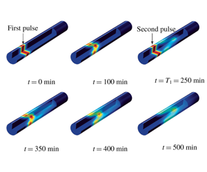
(iii) Solutions to the effective convection–dispersion equation should be superposable in the sense defined by Taylor (Reference Taylor1959). This criterion is based on a physical desideratum outlined by Taylor (Reference Taylor1959). Essentially, the argument was that if a new source was injected after some time had elapsed (the ‘two release’ problem), the effective dispersion coefficient should be single valued at points where the two sources overlap. The time-dependent dispersion theories would predict two different values for the dispersion coefficient at such overlapping points, a situation to which Taylor (Reference Taylor1959) objected.
(iv) Whatever the theory for preasymptotic dispersion is, the dispersion coefficient should approach over time the classical asymptotic values that have been developed in the literature. These classical asymptotic values have been scrutinized rigorously for decades; there is little uncertainty in those results.
Our goal in this work is to develop a theory that addresses each of these issues; we seek to make the theory as concrete as possible by expressing results in analytical form when feasible. We neglect reaction, although the methods proposed are extendable to that case (cf. Wang et al. Reference Wang, Li, Wu and An2015). Ultimately, our approach leads to an upscaled equation for a single chemical species that contains a non-conventional source term as follows:
 $$\begin{eqnarray}{\displaystyle \frac{\unicode[STIX]{x2202}\langle c\rangle }{\unicode[STIX]{x2202}t}}=D^{\ast }(t){\displaystyle \frac{\unicode[STIX]{x2202}^{2}\langle c\rangle }{\unicode[STIX]{x2202}z^{2}}}-U{\displaystyle \frac{\unicode[STIX]{x2202}\langle c\rangle }{\unicode[STIX]{x2202}z}}+s^{\ast }(z,t).\end{eqnarray}$$
 Here,  $c$ is the concentration of the solute, the angled brackets indicate cross-section average, $D^{\ast }$ is the effective dispersion coefficient, $U$ is the cross-sectional-averaged longitudinal velocity and $s^{\ast }$ is a non-conventional source term that is exponentially decaying in time; $z$ and $t$ are the independent variables representing space and time, respectively. While this form for a macroscale balance equation may seem unusual, the source term $s^{\ast }$ is an essential component that arises directly from the upscaling analysis. This source term creates an overall balance that meets the set of criteria defined above for a well-structured dispersion process.
The remainder of the manuscript is outlined as follows. In the next section, we give an overview of the literature on Taylor dispersion, with a specific focus on methods that have been developed to handle early time evolution from the initial conditions. This is followed by a presentation of the microscale physics in § 3. In § 4, we define the upscaling process. In § 5, the problem of closure is presented and integral closure solutions are described. The closed problem is described in § 6; in this section we also define the effective dispersion coefficient,  $D^{\ast }$, and source term, $s^{\ast }$, and provide explicit analytical solutions for these quantities. In § 7, we compute solutions to the dispersion problem for three different initial configurations, and compare the results derived from the upscaled model with those derived from numerical simulations (NS) computed at the microscale. Both averaged concentrations and spatial moments are compared. In § 8 we provide some discussion of the results of the theory applied to several interesting initial conditions. In § 9, we specifically address the application of the upscaled balance equation to conditions where the problem superposition is of interest. Finally, in § 10 a list of conclusions is presented. Supplementary materials available at https://doi.org/10.1017/jfm.2020.56 have been generated to support this work; these materials include specific details regarding error analysis, correspondences between the theory developed here and infinite-order expansion methods and a list of notation.
2 Background
In this section, we review a subset of the work conducted on the Taylor dispersion problem. An exhaustive literature review on the subject is challenging because of the volume of literature represented by this topic; therefore, our review is focused specifically on studies that seek to provide solutions for early-time behaviour. In the material that follows, we define the Péclet number by
 $$\begin{eqnarray}Pe={\displaystyle \frac{Ua}{{\mathcal{D}}}},\end{eqnarray}$$
 where  ${\mathcal{D}}$ is the molecular diffusion coefficient, and $a$ is the radius of the tube. Most studies of Taylor dispersion have adopted this definition for the Péclet number; it can be thought of as the ratio of the convective to the (radial) diffusive fluxes. This is slightly different from the work of Taylor (Reference Taylor1953), who used the ratio of the diffusive to convective time scales (this difference is discussed in subsequent sections).
2.1 Review of the literature
For the purposes of the review below, early time is qualitatively defined as the transient time period during which the relaxation of the initial configuration of the solute is important to the dynamics of the Taylor dispersion process. It is possible to broadly characterize the different mathematical approaches for describing Taylor dispersion in the transient, early-time regime as outlined below.
(i) Kramers–Moyal-like expansions. By far the most popular approach has been the proposition that the macroscale solution can be expressed as an infinite series of spatial derivatives of the average concentration. Several variations of this approach have been attempted, and they are represented in the works of Gill et al. (Gill & Sankarasubramanian Reference Gill and Sankarasubramanian1970, Reference Gill and Sankarasubramanian1971), Chatwin (O’Hara Reference O’Hara1969; Chatwin Reference Chatwin1970, Reference Chatwin1972), Degance & Johns (Reference Degance and Johns1978a,Reference Degance and Johnsb) and Mauri (Reference Mauri1991). Balakotaiah, Chang & Smith (Reference Balakotaiah, Chang and Smith1995) used centre manifold theory to develop a macroscale formulation that is identical to that of Gill & Sankarasubramanian (Reference Gill and Sankarasubramanian1970). The resolution of the centre manifold model was improved by Watt & Roberts (Reference Watt and Roberts1996) by constructing a multi-mode model for dispersion in channels. These authors considered a two-component model that follows the same trend of thought of the zonal models by Chikwendu & Ojiakor (Reference Chikwendu and Ojiakor1985), Chikwendu (Reference Chikwendu1986a,Reference Chikwendub). The work by Yu (Reference Yu1976, Reference Yu1979) is interesting in that it began as a formal eigenfunction expansion for an unsimplified version of the convection–diffusion equation by assuming that expansions in Bessel functions were possible. After a formal integral solution was developed, the term arising from the initial conditions was discarded, and the remaining integrations of the Bessel functions were expanded in a power series. The result was a solution in an infinite series of derivatives of all orders, much like the Kramers–Moyal-type expansions discussed above. Although originally promoted as being more capable than the models of Gill & Sankarasubramanian (Reference Gill and Sankarasubramanian1970), a sequence of comments (Gill & Subramanian Reference Gill and Subramanian1980; Yu Reference Yu1980) established that the two methods are, at least to order 3, identical. The works by Westerterp, Dil’man & Kronberg (Reference Westerterp, Dil’man and Kronberg1995) and Kronberg, Benneker & Westerterp (Reference Kronberg, Benneker and Westerterp1996) are of this type, but in that work the iterative process was truncated at order 2. One unique feature of those works is that mixed derivative terms were maintained, and this ultimately led to a macroscale form that had hyperbolic (rather than parabolic) features. We note that the work by Gill & Sankarasubramanian (Reference Gill and Sankarasubramanian1970) also derived hyperbolic terms in their approach, but ultimately eliminated those terms on the basis of their assumed macroscale form. More recently, Wu & Chen (Reference Wu and Chen2014) used an expansion involving spatial derivatives up to ninth order. Although their results compared well with previously reported numerical results, they did not recognize that their solutions included significant negative concentrations outside of a limited domain. This kind of error was corrected in a later paper (Wang & Chen Reference Wang and Chen2016). Other works (Mercer & Roberts Reference Mercer and Roberts1990, Reference Mercer and Roberts1994; Balakotaiah et al. Reference Balakotaiah, Chang and Smith1995) also considered higher-order expansions and addressed the issue of negative concentrations.
(ii) Direct solutions. In the direct solutions, the focus has been to solve the convection–diffusion mass balance equation in the tube directly using an eigenfunction expansion. This is a challenging task, because the conventional methods (e.g. separation of variables) used to determine closed-form expressions for the Green’s function do not work with this problem, primarily because the convection term mixes both radial and longitudinal independent variables. The first direct solutions appear to be those of Philip (Reference Philip1963). For that work, however, the solution sought was initially of the form of a diffusion equation (similar to the more general approach of Gill & Sankarasubramanian (Reference Gill and Sankarasubramanian1970)), which automatically excluded certain forms of the initial condition (with roughly the same reasoning discussed by Degance & Johns (Reference Degance and Johns1980)). The paper proposed a solution as a series of the confluent hypergeometric functions  $_{1}F_{1}$. The papers by Tseng & Besant (Reference Tseng and Besant1970, Reference Tseng and Besant1972) assumed the same solution as did Philip (Reference Philip1963) (and were subject to the same restrictions), but managed to find simplifications that yielded solutions in terms of Bessel $\text{J}_{0}$ functions, the roots of the Bessel $\text{J}_{1}$ function and the error function. In the work by Stokes & Barton (Reference Stokes and Barton1990), a Fourier transformation method was used, but the results had to be inverted numerically; as such, it is difficult to compare these results with other efforts.
(iii) Asymptotic (perturbation) solutions. A number of perturbation-type solutions have been proposed, and it is not possible to cleanly categorize solutions from other approaches as being free from perturbation-like arguments. However, more classical perturbation-type expansions have been investigated by Vrentas & Vrentas (Reference Vrentas and Vrentas1988, Reference Vrentas and Vrentas2000). The paper by Lighthill (Reference Lighthill1966) is of this form, as was the extension proposed by Chatwin (Reference Chatwin1976, Reference Chatwin1977); both of these solutions required the time to be small compared to a characteristic diffusive time scale. Fife & Nicholes (Reference Fife and Nicholes1975) conducted a conventional perturbation analysis, but, importantly, recognized the potential influence of initial source terms, which is somewhat unique. Phillips and Kaye examined the asymptotic (but direct) solutions for  $Pe\rightarrow \infty$ for both large $z$ (Reference Phillips and Kaye1996), and short times (Reference Phillips and Kaye1997); both solutions neglected longitudinal diffusion. Such solutions have generally been very successful when used in their range of validity (which generally involves either long or short times, and/or large or small Péclet numbers).
(iv) Moment methods. The early paper by Aris (Reference Aris1956) presented the first moment-based method for Taylor dispersion. Although the paper purported to eliminate the constraints proposed by Taylor (Reference Taylor1954), in fact the method is technically only suitable for asymptotic estimates of the dispersion coefficient, although some transient results were presented for particular initial conditions. Moment methods focus on determining the spatial moments of the concentration field rather than its mean value (which, quite usefully, simplifies the analysis), often with the tacit assumption that the effective parameters of the averaged mass balance equation can be determined directly from the moments. Again, it is difficult to categorize approaches as uniquely moment based, since many approaches compute moments regardless of the underpinning mathematical methods used. A number of researchers have extended moment method into the preasymptotic regime, including the works of Horn (Reference Horn1971), Chatwin (Reference Chatwin1977), Degance & Johns (Reference Degance and Johns1978b), Latini & Bernoff (Reference Latini and Bernoff2001) and Dentz & Carrera (Reference Dentz and Carrera2007). The moment technique has become particularly popular in describing Taylor-like flows in stratified media (e.g. Fried & Combarnous Reference Fried and Combarnous1971; Lake & Hirasaki Reference Lake and Hirasaki1981; Valocchi Reference Valocchi1989), downstream contaminant release in rivers (Smith Reference Smith1984), among many others. The method inherently assumes that a finite number of moments suitably defines the transport behaviour of the system, an assumption that is technically only true for specific initial conditions or in the near-asymptotic regime (this issue is discussed further in § 2.2).
(v) Non-local formulations. Few non-local formulations (containing terms with either time or space integrations in the transport equation) have been proposed for this problem. Although not specific to the Taylor problem, the work of Deng & Cushman (Reference Deng and Cushman1995) is of this type, and somewhat set the standard for non-local equations of the convection–dispersion type (however, in a more general context, the work of Eringen (Reference Eringen1978) was ground-breaking for non-local balance equations). The paper by Wood & Valdés-Parada (Reference Wood and Valdés-Parada2013) also proposed non-local formulations from the volume averaging perspective, although they were also not specific to the Taylor dispersion problem. In the report of Smith (Reference Smith1981a), one of the first non-local formulations to the Taylor problem was outlined. The developments of that paper were also guided by a Kramers–Moyal-type expansion, and thus lead to hyperbolic expressions with mixed derivatives as well as more general convolution-integral expressions (depending on the order of the truncation, and where in the analysis the truncations are performed). The work by Jones & Young (Reference Jones and Young1994) also used a variation of this approach, but in an asymptotic framework (also capitalizing on the centre manifold theory). In this theory, the results were able to capture some features of the early-time behaviour, but were not able to capture exponentially decaying-in-time modes; most likely, this was because the initial condition was not represented as a source term in the averaged equation.
(vi) Formulations that include an initial condition source. Most studies on Taylor dispersion have not been overly interested in the relaxation of the initial condition; often, the only initial conditions examined are either uniform pulses, or delta-like impulses (Vedel, Hovad & Bruus Reference Vedel, Hovad and Bruus2014). Few papers have been developed with the realization that the initial condition can manifest as a decaying source term in the averaged mass balance when more complex initial conditions are considered. Philip (Reference Philip1963) was aware that essentially forcing the upscaled mass balance to be of a convection–dispersion form would limit the choices available for the initial condition. The importance of the initial condition was also apparent to Lighthill (Reference Lighthill1966), although he was not able to complete a general analysis for his solution. In a series of papers, Gill and Sankarasubramanian derived macroscale models for unsteady solute dispersion considering uniform (Gill & Sankarasubramanian Reference Gill and Sankarasubramanian1970) and non-uniform (Gill & Sankarasubramanian Reference Gill and Sankarasubramanian1971; Sankarasubramanian & Gill Reference Sankarasubramanian and Gill1973) slugs as initial conditions. Connections between these works and the developments presented here are derived in additional detail in the supplementary material. The work by Yu (Reference Yu1979) began by including the initial condition in the macroscale balance, but later this term was dropped resulting in a final theory that does not have a source arising from the initial configuration of the system. In the papers by Degance and Johns (Reference Degance and Johns1978b, Reference Degance and Johns1980), the influence of the initial condition appeared as part of the theory. However, this work specifically considered a subset of possible initial conditions that work with the theory; in particular, separable product forms for the initial condition function were allowable, but sums of any two such functions were excluded (Degance & Johns Reference Degance and Johns1978a, § 4). Smith (Reference Smith1981b) identified and described three stages of unsteady dispersion from a point source using a ray-tracing method. Haber & Mauri (Reference Haber and Mauri1988) used a stochastic Markovian particle approach to examine the role of the initial condition; explicit asymptotic solutions were derived that illustrated that the observed dispersion coefficient depended upon the initial location of the particles. From a moment-based approach, the paper by Dentz & Carrera (Reference Dentz and Carrera2007) similarly considered delta-type impulses placed near the centre versus the wall initially; in that work, a distinction between local and global dispersion was defined to distinguish between the dispersion of a single delta impulse versus the dispersion observed for an extended source. Meng & Yang (Reference Meng and Yang2018) adopted a perspective similar to that of Dentz & Carrera (Reference Dentz and Carrera2007), but solved for the effective dispersion coefficient via eigenfunction expansions. They also found that the dispersion coefficient was a function of the initial configuration. In a sequence of two papers, Wood (Reference Wood2009, equations (17) and (29)) and Wood & Valdés-Parada (Reference Wood and Valdés-Parada2013) developed theories that explicitly included the influence of the initial condition as a source term in the averaged mass balance equation; this process was then used by Ostvar & Wood (Reference Ostvar and Wood2016) to describe the average diffusion and reaction from an initial (unmixed) configuration. Independently, Balakotaiah & Ratnakar (Reference Balakotaiah and Ratnakar2010) also developed balance expressions specifically for the Taylor dispersion problem in which source terms arising from the initial conditions were employed; a Kramers–Moyal-like expansion was used, but truncated at second order. This model had the ability to predict significant skewness in the distribution (Ratnakar & Balakotaiah Reference Ratnakar and Balakotaiah2011). While not unique to the models discussed, the prediction of skewness is an important check on the physics of the solution, since skewness should become non-zero at early times (even if the initial condition is symmetric), and it should asymptotically approach zero in the long-time regime.
In the remainder of the background section, we elaborate a little more on two specific issues that arise in the previous work summarized above: (i) The use of infinite-order (Kramers–Moyal-type) expansions, and (ii) the neglect of source terms arising from the initial condition.
2.2 Comments regarding Kramers–Moyal-type expansions
There are two significant problems with the infinite Kramers–Moyal-type expansions. First, because of the specific macroscale representation that is chosen, the resulting theory generates dispersion coefficients that may depend upon the initial condition (Degance & Johns Reference Degance and Johns1980). Second, research on the positivity of such series was apparently not known to progenitors of this approach. It is now known that such series either (i) converge exactly at second order and are strictly positive, or (ii) require all terms in order to converge and remain strictly positive (Marcinkiewicz Reference Marcinkiewicz1939; Pawula Reference Pawula1967). Although Kramers–Moyal expansions do (under appropriate conditions) converge, they do not converge in a highly physical way when strictly positive results are sought (as in the case of concentration). In other words, any finite truncation of a Kramers–Moyal expansion of order greater than two generates results that are negative in some parts of the domain. This problem has been discussed in the literature (e.g. Risken & Vollmer Reference Risken and Vollmer1979), but it is not generally well recognized in many disciplines outside of physics. The fact that negative concentrations are essentially guaranteed to occur for truncated expansions does not negate the usefulness of such expansions (Risken & Vollmer Reference Risken and Vollmer1979), but it does demand careful analysis and cautiousness when interpreting results. The problem of negative concentrations is most acute at early times (cf. Wood & Valdés-Parada (Reference Wood and Valdés-Parada2013, § 7)). Some of the problems associated with the Kramers–Moyal expansion can be eliminated by the recognition that such expansions can often be represented by non-local convolution expressions (Mercer & Roberts Reference Mercer and Roberts1990, Reference Mercer and Roberts1994). It is easy to show that a general non-local transport formulation can be written as an infinite-order expansion of local derivatives (this is illustrated in the supplementary material), although the converse of this is not always true. However, given that the macroscale equation form adopted in most of these examples is posited as an ansatz (e.g. Gill & Sankarasubramanian (Reference Gill and Sankarasubramanian1970, equations (5) and (8))), then it might be reasonable to start directly with the convolution rather than the series form. For the specific problem of Taylor dispersion investigated in this paper, we are able to show that the solution is generally of a convolution form, giving further support that this kind of approach might have a stronger physical basis. Regardless, the non-local formulations generally avoid the problems associated with negative concentrations, and, in appropriate limits, reduce to more familiar local macroscale equations.
2.3 Influence of the initial conditions
As the review of the literature above suggests, the importance of the initial configuration at early times has been identified (although not resolved) previously. The problem can be most easily thought about in the context of layered media which, although not a tube, is still frequently represented as a Taylor dispersion process, (e.g. Fried & Combarnous Reference Fried and Combarnous1971; Gelhar, Gutjahr & Naff Reference Gelhar, Gutjahr and Naff1979; Lake & Hirasaki Reference Lake and Hirasaki1981; Chikwendu & Ojiakor Reference Chikwendu and Ojiakor1985; Chikwendu Reference Chikwendu1986a,Reference Chikwendub). Consider an initially uniform slug of solute in a system of horizontal layers of alternating high and low conductivity that is transported by a forward-flow/reverse-flow transport cycle. If a constant pressure gradient is applied for a short period of time such that the mean flow is right to left, the solute is displaced more in the high-velocity layers than in the low ones, leading to a spatially staggered final condition. Now, suppose the flow is stopped, and the pressure gradient reversed. The staggered configuration is the initial condition for a new transport process. Assuming that the total time interval is small enough so that transverse diffusion does not spread the solute very much between layers, the resulting motion is largely reversible. Upon reversing the flow field, a seemingly spread-out initial condition converges to become more organized (and less spread out). In the limit of zero diffusion, the final result of this first forward and then reversed transport would be exactly identical to the initial condition.
This kind of process creates some conceptual problems. Seemingly, the second moment of the process described above first increases and then, upon flow reversal, decreases in time. If one interprets the effective dispersion coefficient as being the classical one half of the time rate of change of the second spatial moment, then one predicts a negative dispersion coefficient for the second half of the cycle. This problem has been recognized in part as one that involves the distinction between spreading and mixing (e.g. Dentz & Carrera Reference Dentz and Carrera2007). However, one is still left with a macroscale equation that contains an apparent dispersion coefficient that can be negative under some conditions. The problem is of the inverse heat equation type, which is known to be ill posed (Weber Reference Weber1981). The solutions to such problems are lossy in general and can lead to significant problems in interpretation. Of more importance, however, is that such expressions are inconsistent with macroscale thermodynamics (Gray & Miller Reference Gray and Miller2009; Gray & Miller Reference Gray and Miller2014, chap. 10; Miller et al. Reference Miller, Valdés-Parada, Ostvar and Wood2018). Thus, if one hopes to solve problems in a manner consistent with the thermodynamics appropriate to the upscaled system, a negative dispersion coefficient is not a suitable choice. The use of higher-order diffusive-type equations (such as the method of Gill & Sankarasubramanian (Reference Gill and Sankarasubramanian1970)) does not entirely remediate this problem. Although there are more degrees of freedom in these kinds of expansions to accommodate the influence of initial conditions, the fundamental problem is that the initial conditions enter the problem as source terms that are independent of the spatial derivatives of the average concentration. Thus, some initial configurations, when forced to fit a transport equation that contains no term representing a source, may predict non-physical behaviour for the dispersion coefficient, depending upon the underlying theory.
3 Problem formulation
One of the primary purposes of this work is to examine the early-time dispersion process in the context of an averaging theory, but maintaining the influence of the initial configuration throughout the averaging process. Our proposed model seeks to remedy the problems identified above by assuring that both the concentration and the dispersion coefficient remain positive over the entire (time and space) domain of the problem.
A subset of the domain,  ${\mathcal{V}}$, geometry indicating coordinate directions and example vectors. Each vector (e.g. $\boldsymbol{r}$, $\boldsymbol{z}$ and $\boldsymbol{y}$) can be expressed in a cylindrical coordinate system for analytical or numerical computations. Note the distinction between the coordinates $r$ and $z$ versus the vectors $\boldsymbol{r}$ and $\boldsymbol{z}$. In this figure and the figures that follow, the aspect ratio of the radial, $r$, to longitudinal, $z$, coordinates has been increased to improve the presentation of results.

We consider passive transport of a chemical species in a cylindrical domain specified by  $\boldsymbol{r}\in {\mathcal{V}}$, where $\boldsymbol{r}\equiv (r,\unicode[STIX]{x1D703},z)$ (figure 1). For the cases considered in this analysis, we assume that the solute does not interact significantly with the external boundaries perpendicular to the axis of the tube. Thus, for concreteness, we set the external planes perpendicular to the tube axis at locations $z\rightarrow \pm \infty$, respectively. The initial solute distribution is assumed to be a known function of position denoted by $\unicode[STIX]{x1D711}(r,\unicode[STIX]{x1D703},z)$. The transport equations at the microscale for a solute in terms of molar concentrations can be written in cylindrical coordinates as
Microscale mass balance
 $$\begin{eqnarray}\displaystyle & \displaystyle {\displaystyle \frac{\unicode[STIX]{x2202}c}{\unicode[STIX]{x2202}t}}+v_{z}(r){\displaystyle \frac{\unicode[STIX]{x2202}c}{\unicode[STIX]{x2202}z}}={\displaystyle \frac{{\mathcal{D}}}{r}}{\displaystyle \frac{\unicode[STIX]{x2202}}{\unicode[STIX]{x2202}r}}\left(r{\displaystyle \frac{\unicode[STIX]{x2202}c}{\unicode[STIX]{x2202}r}}\right)+{\displaystyle \frac{{\mathcal{D}}}{r^{2}}}{\displaystyle \frac{\unicode[STIX]{x2202}^{2}c}{\unicode[STIX]{x2202}\unicode[STIX]{x1D703}^{2}}}+{\mathcal{D}}{\displaystyle \frac{\unicode[STIX]{x2202}^{2}c}{\unicode[STIX]{x2202}z^{2}}}, & \displaystyle\end{eqnarray}$$
 $$\begin{eqnarray}\displaystyle & \displaystyle \text{B.C.1}\quad -{\mathcal{D}}{\displaystyle \frac{\unicode[STIX]{x2202}c}{\unicode[STIX]{x2202}r}}=0\quad \text{at }r=0,a, & \displaystyle\end{eqnarray}$$
 $$\begin{eqnarray}\displaystyle & \displaystyle \text{B.C.2a}\quad c\rightarrow 0\quad z\rightarrow \pm \infty , & \displaystyle\end{eqnarray}$$
 $$\begin{eqnarray}\displaystyle & \displaystyle \text{B.C.2b}\quad -{\mathcal{D}}{\displaystyle \frac{\unicode[STIX]{x2202}c}{\unicode[STIX]{x2202}z}}\rightarrow 0\quad z\rightarrow \pm \infty , & \displaystyle\end{eqnarray}$$
 $$\begin{eqnarray}\displaystyle & \displaystyle \text{I.C.}\quad c(r,\unicode[STIX]{x1D703},z,0)=\unicode[STIX]{x1D711}(r,\unicode[STIX]{x1D703},z). & \displaystyle\end{eqnarray}$$ $\unicode[STIX]{x1D703}$-symmetric velocity field given by the well-known expression depending only on the distance, $r$, from the centreline of the tube
  $$\begin{eqnarray}v_{z}(r)=2U\left(1-{\displaystyle \frac{r^{2}}{a^{2}}}\right).\end{eqnarray}$$
With this information, the problem is fully specified.
4 Upscaling process
4.1 Preliminaries
In this paper, we upscale (or coarse grain) the system concentration field dynamics by simple spatial averaging against a weighting function. The underlying assumption in this approach is that the system can be sensibly represented by governing equations at more than one scale of resolution due to the multiscale (in space, time or both) characteristics of the system. Practically, this means that there exist averaging operators that sufficiently smooth spatial fluctuations in concentration such that an averaged behaviour is useful for understanding the system evolution. In this work, the averaging process is a somewhat modified form of volume averaging theory (which is frequently applied to porous materials, (Whitaker Reference Whitaker1999)), but we do not stress this point further.
In the remainder of this paper, we adopt cylindrical coordinates (figure 1); thus, for any function  $\unicode[STIX]{x1D713}$, we have $\unicode[STIX]{x1D713}(\boldsymbol{r})=\unicode[STIX]{x1D713}(r,\unicode[STIX]{x1D703},z)$. The symbol $\boldsymbol{z}$ (set in bold font) is used exclusively to indicate the centroid of the averaging domain; therefore, this vector always has the component form $\boldsymbol{z}=(0,0,z)$. The averaging operator $\langle \cdot \rangle$ for Taylor dispersion is often defined with respect to weighting function $w$ by (Degance & Johns Reference Degance and Johns1978a)
 $$\begin{eqnarray}\langle \unicode[STIX]{x1D713}\rangle |_{(\boldsymbol{z},t)}=\int _{\boldsymbol{r}\in {\mathcal{V}}(\boldsymbol{z})}\unicode[STIX]{x1D713}(\boldsymbol{r},t)w(\boldsymbol{r}-\boldsymbol{z})\,\text{d}V(\boldsymbol{r}).\end{eqnarray}$$
Or, in the cylindrical coordinate system
 $$\begin{eqnarray}\langle \unicode[STIX]{x1D713}\rangle |_{(\boldsymbol{z},t)}=\int _{\unicode[STIX]{x1D701}=-\infty }^{\unicode[STIX]{x1D701}=\infty }\int _{\unicode[STIX]{x1D703}=0}^{\unicode[STIX]{x1D703}=2\unicode[STIX]{x03C0}}\int _{r=0}^{r=a}\unicode[STIX]{x1D713}(r,\unicode[STIX]{x1D703},\unicode[STIX]{x1D701},t)w(r,\unicode[STIX]{x1D703},\unicode[STIX]{x1D701}-z)r\,\text{d}r\,\text{d}\unicode[STIX]{x1D703}\,\text{d}\unicode[STIX]{x1D701}.\end{eqnarray}$$
 For this work, we adopt the classical area average, so that  $w(\boldsymbol{r}-\boldsymbol{z})=w(r,\unicode[STIX]{x1D703},\unicode[STIX]{x1D701}-z)=1/(\unicode[STIX]{x03C0}a^{2})\unicode[STIX]{x1D6FF}(z-\unicode[STIX]{x1D701})$, which yields the conventional area average (note, other weighting functions have been adopted for Taylor dispersion, cf. Degance & Johns (Reference Degance and Johns1978a))
 $$\begin{eqnarray}\langle \unicode[STIX]{x1D713}\rangle |_{(\boldsymbol{z},t)}={\displaystyle \frac{1}{\unicode[STIX]{x03C0}a^{2}}}\int _{\unicode[STIX]{x1D703}=0}^{\unicode[STIX]{x1D703}=2\unicode[STIX]{x03C0}}\int _{r=0}^{r=a}\unicode[STIX]{x1D713}(r,\unicode[STIX]{x1D703},z,t)r\,\text{d}r\,\text{d}\unicode[STIX]{x1D703}.\end{eqnarray}$$
 We refer to the filtered functions  $\langle \unicode[STIX]{x1D713}\rangle$ as macroscale quantities to distinguish them from their microscale counterparts, $\unicode[STIX]{x1D713}$.
In addition to the definition of the averaging operator, it is also useful to define the following decompositions:
 $$\begin{eqnarray}\displaystyle & c(\boldsymbol{r},t)=\langle c\rangle |_{(\boldsymbol{z},t)}+\tilde{c}(\boldsymbol{r},t) & \displaystyle\end{eqnarray}$$
 $$\begin{eqnarray}\displaystyle & v_{z}(r)=U+\tilde{v}_{z}(r). & \displaystyle\end{eqnarray}$$ $U=\langle v_{z}\rangle |_{\boldsymbol{z}}$ whereas $\tilde{c}$ and $\tilde{v}_{z}$ denote spatial deviations from their corresponding averages. Note that these deviations are defined in a manner that is different from the conventional definition used in the volume averaging theory. The above decompositions are the same as those proposed by Gray (Reference Gray1975); that is, the deviations in each averaging domain are defined relative to the value of the average at the longitudinal centroid of the tube. There are some advantages to this definition; in particular, we have the following identities:
  $$\begin{eqnarray}\displaystyle & \langle \tilde{c}\rangle |_{(\boldsymbol{z},t)}=0, & \displaystyle\end{eqnarray}$$
 $$\begin{eqnarray}\displaystyle & \langle \tilde{v}_{z}\rangle |_{\boldsymbol{z}}=0. & \displaystyle\end{eqnarray}$$
4.2 Averaging the microscale balance equation
To obtain the macroscale mass balance equation, we apply the averaging operator defined above to the microscale balance. Note that, although we have been careful to explicitly list the independent variables in the definitions above, we do so in the remainder of the paper only when it is necessary for emphasis or clarity. Upon applying the averaging operator (4.3) to the microscale mass balance equations, the upscaled problem takes the form
 $$\begin{eqnarray}\displaystyle & \displaystyle {\displaystyle \frac{\unicode[STIX]{x2202}\langle c\rangle }{\unicode[STIX]{x2202}t}}={\mathcal{D}}{\displaystyle \frac{\unicode[STIX]{x2202}^{2}\langle c\rangle }{\unicode[STIX]{x2202}z^{2}}}-U{\displaystyle \frac{\unicode[STIX]{x2202}\langle c\rangle }{\unicode[STIX]{x2202}z}}-\left\langle \tilde{v}_{z}{\displaystyle \frac{\unicode[STIX]{x2202}\tilde{c}}{\unicode[STIX]{x2202}z}}\right\rangle , & \displaystyle\end{eqnarray}$$
 $$\begin{eqnarray}\displaystyle & \displaystyle \text{B.C. Macro 1a}\quad \langle c\rangle |_{(z,t)}=0\quad z\rightarrow \pm \infty , & \displaystyle\end{eqnarray}$$
 $$\begin{eqnarray}\displaystyle & \displaystyle \text{B.C. Macro 1b}\quad -{\mathcal{D}}\left.{\displaystyle \frac{\unicode[STIX]{x2202}\langle c\rangle }{\unicode[STIX]{x2202}z}}\right|_{(z,t)}=0\quad z\rightarrow \pm \infty , & \displaystyle\end{eqnarray}$$
 $$\begin{eqnarray}\displaystyle & \displaystyle \text{I.C.1}\quad \langle c\rangle |_{(z,0)}=\langle \unicode[STIX]{x1D711}\rangle |_{z}. & \displaystyle\end{eqnarray}$$
Several steps have been taken into account in order to derive (4.6a). First, interchange of the time derivative and the averaging operator is allowed within the accumulation term due to the fact that the averaging domain does not change with time. Thus we have
 $$\begin{eqnarray}\left\langle {\displaystyle \frac{\unicode[STIX]{x2202}c}{\unicode[STIX]{x2202}t}}\right\rangle ={\displaystyle \frac{\unicode[STIX]{x2202}\langle c\rangle }{\unicode[STIX]{x2202}t}}.\end{eqnarray}$$
Directing our attention to the diffusion term, the microscale boundary conditions lead to the identity
 $$\begin{eqnarray}\displaystyle \left\langle {\mathcal{D}}{\displaystyle \frac{\unicode[STIX]{x2202}^{2}c}{\unicode[STIX]{x2202}z^{2}}}\right\rangle ={\mathcal{D}}{\displaystyle \frac{\unicode[STIX]{x2202}^{2}\langle c\rangle }{\unicode[STIX]{x2202}z^{2}}}. & & \displaystyle\end{eqnarray}$$
For the convection term, we have (on the basis of (4.4a)–(4.5b))
 $$\begin{eqnarray}\displaystyle \left\langle v_{z}{\displaystyle \frac{\unicode[STIX]{x2202}c}{\unicode[STIX]{x2202}z}}\right\rangle =U{\displaystyle \frac{\unicode[STIX]{x2202}\langle c\rangle }{\unicode[STIX]{x2202}z}}+\left\langle \tilde{v}_{z}{\displaystyle \frac{\unicode[STIX]{x2202}\tilde{c}}{\unicode[STIX]{x2202}z}}\right\rangle . & & \displaystyle\end{eqnarray}$$
 Finally, for the two macroscopic boundary conditions given in (4.6b) and (4.6c), we have imposed the condition that  $\tilde{c}(r,\unicode[STIX]{x1D703},z)\rightarrow 0$ and $\unicode[STIX]{x2202}\tilde{c}/\unicode[STIX]{x2202}z(r,\unicode[STIX]{x1D703},z)\rightarrow 0$ as $|z|\rightarrow \infty$. Up to this point, we have employed no approximations to the result; the averaged model represented by (4.6a)–(4.6d) is exact, at least to the extent that the original microscale balance equations are valid.
5 Deviation equations
Equation (4.6a) is unclosed because it is not expressed exclusively in terms of the average concentration. To close the problem, a set of ancillary balances are developed for the microscale deviations of  $\tilde{c}$. Motivated by the definition of the decompositions, we develop the deviation balance by subtracting the averaged equation (4.6a) from the microscale equation (3.1a). In addition, the boundary conditions can be developed by using the decomposition given by (4.4a), and the initial condition is determined by subtracting the averaged initial condition from its microscale counterpart. The resulting equations can be written as follows:
 $$\begin{eqnarray}\displaystyle & & \displaystyle \underbrace{{\displaystyle \frac{\unicode[STIX]{x2202}\tilde{c}}{\unicode[STIX]{x2202}t}}}_{accumulation}+\underbrace{U{\displaystyle \frac{\unicode[STIX]{x2202}\tilde{c}}{\unicode[STIX]{x2202}z}}}_{\substack{ mean \\ convection}}+\underbrace{\tilde{v}_{z}{\displaystyle \frac{\unicode[STIX]{x2202}\tilde{c}}{\unicode[STIX]{x2202}z}}}_{\substack{ deviation \\ convection}}-\underbrace{\left\langle \tilde{v}_{z}{\displaystyle \frac{\unicode[STIX]{x2202}\tilde{c}}{\unicode[STIX]{x2202}z}}\right\rangle }_{\substack{ non\text{-}local \\ convection}}\nonumber\\ \displaystyle & & \displaystyle \quad -\underbrace{{\displaystyle \frac{{\mathcal{D}}}{r}}{\displaystyle \frac{\unicode[STIX]{x2202}}{\unicode[STIX]{x2202}r}}\left(r{\displaystyle \frac{\unicode[STIX]{x2202}\tilde{c}}{\unicode[STIX]{x2202}r}}\right)-{\displaystyle \frac{{\mathcal{D}}}{r^{2}}}{\displaystyle \frac{\unicode[STIX]{x2202}^{2}\tilde{c}}{\unicode[STIX]{x2202}\unicode[STIX]{x1D703}^{2}}}-{\mathcal{D}}{\displaystyle \frac{\unicode[STIX]{x2202}^{2}\tilde{c}}{\unicode[STIX]{x2202}z^{2}}}}_{diffusion}=-\underbrace{\tilde{v}_{z}{\displaystyle \frac{\unicode[STIX]{x2202}\langle c\rangle }{\unicode[STIX]{x2202}z}}}_{\substack{ local \\ convective\,source}},\end{eqnarray}$$
 $$\begin{eqnarray}\text{B.C.1}\quad -{\mathcal{D}}{\displaystyle \frac{\unicode[STIX]{x2202}\tilde{c}}{\unicode[STIX]{x2202}r}}=0\quad \text{at }r=0,a,\end{eqnarray}$$
 $$\begin{eqnarray}\text{B.C.2b}\quad \tilde{c}\rightarrow 0\quad z\rightarrow \pm \infty ,\end{eqnarray}$$
 $$\begin{eqnarray}\text{B.C.2b}\quad -{\mathcal{D}}{\displaystyle \frac{\unicode[STIX]{x2202}\tilde{c}}{\unicode[STIX]{x2202}z}}\rightarrow 0\quad z\rightarrow \pm \infty ,\end{eqnarray}$$
 $$\begin{eqnarray}\text{I.C.1}\quad \tilde{c}(r,\unicode[STIX]{x1D703},z,0)=\underbrace{\tilde{\unicode[STIX]{x1D711}}(r,\unicode[STIX]{x1D703},z)}_{source}\quad (r,\unicode[STIX]{x1D703},z)\in {\mathcal{V}}.\end{eqnarray}$$
 For the developments that follow, it is convenient to adopt a Lagrangian perspective based upon an inertial frame of reference that moves with the centre of mass with the system. To this end, let us define  $z^{\prime }=z-Ut$, $t^{\prime }=t$, so that
 $$\begin{eqnarray}{\displaystyle \frac{\unicode[STIX]{x2202}}{\unicode[STIX]{x2202}t}}={\displaystyle \frac{\unicode[STIX]{x2202}}{\unicode[STIX]{x2202}t^{\prime }}}+U{\displaystyle \frac{\unicode[STIX]{x2202}}{\unicode[STIX]{x2202}z^{\prime }}}.\end{eqnarray}$$
We omit the explicit writing of the prime coordinates in the developments that follow to keep the notation simple. Making the translation to Lagrangian coordinates, the governing differential equation for the concentration deviations becomes
 $$\begin{eqnarray}{\displaystyle \frac{\unicode[STIX]{x2202}\tilde{c}}{\unicode[STIX]{x2202}t}}+\tilde{v}_{z}{\displaystyle \frac{\unicode[STIX]{x2202}\tilde{c}}{\unicode[STIX]{x2202}z}}-\left\langle \tilde{v}_{z}{\displaystyle \frac{\unicode[STIX]{x2202}\tilde{c}}{\unicode[STIX]{x2202}z}}\right\rangle -{\displaystyle \frac{{\mathcal{D}}}{r}}{\displaystyle \frac{\unicode[STIX]{x2202}}{\unicode[STIX]{x2202}r}}\left(r{\displaystyle \frac{\unicode[STIX]{x2202}\tilde{c}}{\unicode[STIX]{x2202}r}}\right)-{\displaystyle \frac{{\mathcal{D}}}{r^{2}}}{\displaystyle \frac{\unicode[STIX]{x2202}^{2}\tilde{c}}{\unicode[STIX]{x2202}\unicode[STIX]{x1D703}^{2}}}-{\mathcal{D}}{\displaystyle \frac{\unicode[STIX]{x2202}^{2}\tilde{c}}{\unicode[STIX]{x2202}z^{2}}}=-\tilde{v}_{z}{\displaystyle \frac{\unicode[STIX]{x2202}\langle c\rangle }{\unicode[STIX]{x2202}z}}.\end{eqnarray}$$
 In (5.3), the term  $\langle \tilde{v}_{z}(\unicode[STIX]{x2202}\tilde{c}/\unicode[STIX]{x2202}z)\rangle$ is non-local in the variable $r$. In this context, we use the term non-local to denote quantities that involve time or space locations in addition to the local ones. Solutions to this balance equation that maintain the non-local term are mathematically tractable, but such solutions remain an active area of research (Chasseigne, Chaves & Rossi Reference Chasseigne, Chaves and Rossi2006; Ignat & Rossi Reference Ignat and Rossi2007; García-Melián & Rossi Reference García-Melián and Rossi2009).
5.1 Elimination of the non-local term
Rather than maintaining the non-local term, our approach is to develop reasonable constraints that allow us to neglect its influence. We do this by establishing characteristic time and length scales, and then developing constraints that indicate when the desired simplification is valid. Although these time and length scales can be given formal, computable definitions (e.g. such as defining them by the integral scale of the fields involved (Wood & Valdés-Parada Reference Wood and Valdés-Parada2013)), formal evaluation of scales is usually not necessary.
For the Taylor dispersion problem, there are several distinct length scales that can be defined. We have identified two important length scales in figure 2. The size of the macroscale length,  $L_{0}$, is described as being approximately the size of the initial condition; however, the validity of this estimate depends upon the particular structure of the initial condition (this is discussed further in § 8.2). The characteristic length of the radial diffusion process is of the order of the tube radius, $a$, for this particular application.
Length scales for the Taylor dispersion problem. The characteristic length associated with the initial solute configuration (illustrated in red) is  $L_{0}$. Because of solute spreading, the generic length scale $L=L(t)$ (defined for all times) is asymptotically larger than $L_{0}$. This figure is meant to be primarily schematic; the actual initial conditions examined in this work are smoothed versions of similar configurations.

The non-local term and the convection term on the left-hand side of (5.3) are of the same order of magnitude. Thus, our desired restriction at this juncture would be to impose
 $$\begin{eqnarray}\tilde{v}_{z}{\displaystyle \frac{\unicode[STIX]{x2202}\tilde{c}}{\unicode[STIX]{x2202}z}}-\left\langle \tilde{v}_{z}{\displaystyle \frac{\unicode[STIX]{x2202}\tilde{c}}{\unicode[STIX]{x2202}z}}\right\rangle \ll {\displaystyle \frac{{\mathcal{D}}}{r}}{\displaystyle \frac{\unicode[STIX]{x2202}}{\unicode[STIX]{x2202}r}}\left(r{\displaystyle \frac{\unicode[STIX]{x2202}\tilde{c}}{\unicode[STIX]{x2202}r}}\right)+\cdots \,.\end{eqnarray}$$
 For complex problems where one wishes to find all possible asymptotically simplified models, there are specific methods and algorithms that can be followed to construct the simplified models (see Yip (Reference Yip1996) for a fuller discussion). Because our restriction is rather simple (and because a full analysis is tedious), we only sketch out the result here. To start, we note that the left-hand side of (5.4) is always less than or equal to  $\tilde{v}_{z}\unicode[STIX]{x2202}\tilde{c}/\unicode[STIX]{x2202}z$. Then, we non-dimensionalize and rearrange the problem as follows (where $Z=z/L_{0}$, $R=r/a$, $\tilde{V}_{z}=\tilde{v}_{z}/U$, $\tilde{C}=\tilde{c}/C_{0}$ and $C_{0}=\max (\tilde{\unicode[STIX]{x1D719}})$):
 $$\begin{eqnarray}\left({\displaystyle \frac{a^{2}U}{L_{0}{\mathcal{D}}}}\right)\tilde{V}_{z}{\displaystyle \frac{\unicode[STIX]{x2202}\tilde{C}}{\unicode[STIX]{x2202}Z}}={\displaystyle \frac{1}{R}}{\displaystyle \frac{\unicode[STIX]{x2202}}{\unicode[STIX]{x2202}R}}\left(R{\displaystyle \frac{\unicode[STIX]{x2202}\tilde{C}}{\unicode[STIX]{x2202}R}}\right)+\cdots \,.\end{eqnarray}$$
 Now, we set  $\unicode[STIX]{x1D700}=a^{2}U/(L_{0}{\mathcal{D}})$. By assumption, $\tilde{V}_{z}\unicode[STIX]{x2202}\tilde{C}/\unicode[STIX]{x2202}Z=\boldsymbol{O}(1)$ and the first term on the right-hand side of (5.5) is of $\boldsymbol{O}(1)$. Examining
 $$\begin{eqnarray}\unicode[STIX]{x1D700}\tilde{V}_{z}{\displaystyle \frac{\unicode[STIX]{x2202}\tilde{c}}{\unicode[STIX]{x2202}Z}}={\displaystyle \frac{1}{R}}{\displaystyle \frac{\unicode[STIX]{x2202}}{\unicode[STIX]{x2202}R}}\left(R{\displaystyle \frac{\unicode[STIX]{x2202}\tilde{c}}{\unicode[STIX]{x2202}R}}\right)+\cdots \,,\end{eqnarray}$$
it is clear that the left-hand side of this expression (and, hence, the left-hand side of (5.4)) can be neglected under the conditions
 $$\begin{eqnarray}{\displaystyle \frac{Ua}{{\mathcal{D}}}}{\displaystyle \frac{a}{L_{0}}}\ll 1\quad \text{or, equivalently, }Pe{\displaystyle \frac{a}{L_{0}}}\ll 1.\end{eqnarray}$$
 The symbols ‘ $\ll$’ and ‘ $\boldsymbol{O}$’ have the conventional meanings adopted in perturbation theory (cf. Bender & Orszag (Reference Bender and Orszag1978, chapters 3.4 and 7)).
A few additional comments are helpful here. First, we note that this approximation may fail at early times if the concentration gradients in the initial condition are large (e.g. step functions); for these early-time solutions, the longitudinal derivative term would need to be maintained. In this work, we consider initial conditions that are reasonably smooth at  $t=0$ (i.e. the first two derivatives are continuous, and correspond to a value of $L_{0}$ that is not much smaller than $a$). Second, this restriction is almost certainly overly severe once the relaxation of the initial condition has progressed for even a relatively small time. Often an approximation such as the inequality (5.4) is valid, even when the two sides are of the same order of magnitude. We describe the results of the error involved in this approximation in additional detail in § 8.2, where we compute it directly to show that the approximation is reasonable for the Péclet numbers investigated in this paper. It is worth noting that the constraint given in (5.7) is identical (except for a factor of 4) to the one imposed by Taylor (Reference Taylor1954)
 $$\begin{eqnarray}Pe_{T}={\displaystyle \frac{a^{2}}{4{\mathcal{D}}}}{\displaystyle \frac{U}{L}}\ll 1.\end{eqnarray}$$
 Here,  $Pe_{T}$ is the Taylor-type Péclet number, which arises naturally when we non-dimensionalize the transport equation. The diffusion time scale arises from considerations of the conventional free-field diffusion relationship with variance $\unicode[STIX]{x1D70E}^{2}=4{\mathcal{D}}t$ (and, hence, $L\sim \sqrt{4{\mathcal{D}}t}$). The convective time scale comes from a simple estimate of the $z-$derivative of the initial condition. With the exception of Taylor (Reference Taylor1954) and Aris (Reference Aris1956), the literature has tended to use the definition that is based on a simple ratio of the convective to diffusive fluxes, of the form (assuming both convective and diffusive fluxes are characterized by a length scale equal to the tube radius, $a$)
$a$)
 $$\begin{eqnarray}Pe={\displaystyle \frac{Ua}{{\mathcal{D}}}}={\displaystyle \frac{4L}{a}}Pe_{T}.\end{eqnarray}$$
 Note that for the simulations reported below with the parameters in table 1,  $Pe_{T}=1$ corresponds to $Pe=80$.
Parameters used in the simulations.

With the approximation given by the inequality (5.4) and the use of Lagrangian coordinates, the resulting set of equations for  $\tilde{c}$ becomes
 $$\begin{eqnarray}\displaystyle & \displaystyle {\displaystyle \frac{\unicode[STIX]{x2202}\tilde{c}}{\unicode[STIX]{x2202}t}}={\displaystyle \frac{{\mathcal{D}}}{r}}{\displaystyle \frac{\unicode[STIX]{x2202}}{\unicode[STIX]{x2202}r}}\left(r{\displaystyle \frac{\unicode[STIX]{x2202}\tilde{c}}{\unicode[STIX]{x2202}r}}\right)+{\displaystyle \frac{{\mathcal{D}}}{r^{2}}}{\displaystyle \frac{\unicode[STIX]{x2202}^{2}\tilde{c}}{\unicode[STIX]{x2202}\unicode[STIX]{x1D703}^{2}}}+{\mathcal{D}}{\displaystyle \frac{\unicode[STIX]{x2202}^{2}\tilde{c}}{\unicode[STIX]{x2202}z^{2}}}-\underbrace{\tilde{v}_{z}(r)\left.{\displaystyle \frac{\unicode[STIX]{x2202}\langle c\rangle }{\unicode[STIX]{x2202}z}}\right|_{(z,t)}}_{source}\quad (r,\unicode[STIX]{x1D703},z)\in {\mathcal{V}}, & \displaystyle\end{eqnarray}$$
 $$\begin{eqnarray}\displaystyle & \displaystyle \text{B.C.1}\quad -{\mathcal{D}}{\displaystyle \frac{\unicode[STIX]{x2202}\tilde{c}}{\unicode[STIX]{x2202}r}}=0\quad \text{at }r=0,a, & \displaystyle\end{eqnarray}$$
 $$\begin{eqnarray}\displaystyle & \displaystyle \text{B.C.2b}\quad \tilde{c}\rightarrow 0\quad z\rightarrow \pm \infty , & \displaystyle\end{eqnarray}$$
 $$\begin{eqnarray}\displaystyle & \displaystyle \text{B.C.2b}\quad -{\mathcal{D}}{\displaystyle \frac{\unicode[STIX]{x2202}\tilde{c}}{\unicode[STIX]{x2202}z}}\rightarrow 0\quad z\rightarrow \pm \infty , & \displaystyle\end{eqnarray}$$
 $$\begin{eqnarray}\displaystyle & \displaystyle \text{I.C.1}\quad \tilde{c}(r,\unicode[STIX]{x1D703},z,0)=\underbrace{\tilde{\unicode[STIX]{x1D711}}(r,\unicode[STIX]{x1D703},z)}_{source}\quad (r,\unicode[STIX]{x1D703},z)\in {\mathcal{V}}. & \displaystyle\end{eqnarray}$$
The above simplified closure problem is a local, linear, non-homogeneous parabolic equation which has well-known solutions. With the conventional assumptions (e.g. boundedness of the initial condition, integrability of the initial condition, smoothness of the boundary conditions, etc.), the solution to the problem for solute transport can be put in an integral formulation as (cf. Polyanin & Nazaikinskii Reference Polyanin and Nazaikinskii2015)
 $$\begin{eqnarray}\displaystyle & & \displaystyle \tilde{c}(r,\unicode[STIX]{x1D703},z,t)\nonumber\\ \displaystyle & & \displaystyle \quad =\int _{\unicode[STIX]{x1D701}=-\infty }^{\unicode[STIX]{x1D701}=\infty }\int _{\unicode[STIX]{x1D717}=0}^{\unicode[STIX]{x1D717}=2\unicode[STIX]{x03C0}}\int _{\unicode[STIX]{x1D70C}=0}^{\unicode[STIX]{x1D70C}=a}G(r,\unicode[STIX]{x1D70C},\unicode[STIX]{x1D703},\unicode[STIX]{x1D717},z,\unicode[STIX]{x1D701},t)\tilde{\unicode[STIX]{x1D711}}(\unicode[STIX]{x1D70C},\unicode[STIX]{x1D717},\unicode[STIX]{x1D701})\unicode[STIX]{x1D70C}\,\text{d}\unicode[STIX]{x1D70C}\,\text{d}\unicode[STIX]{x1D717}\,\text{d}\unicode[STIX]{x1D701}\nonumber\\ \displaystyle & & \displaystyle \qquad -\int _{\unicode[STIX]{x1D70F}=0}^{\unicode[STIX]{x1D70F}=t}\!\int _{\unicode[STIX]{x1D701}=-\infty }^{\unicode[STIX]{x1D701}=\infty }\!\int _{\unicode[STIX]{x1D717}=0}^{\unicode[STIX]{x1D717}=2\unicode[STIX]{x03C0}}\!\int _{\unicode[STIX]{x1D70C}=0}^{\unicode[STIX]{x1D70C}=a}G(r,\unicode[STIX]{x1D70C},\unicode[STIX]{x1D703},\unicode[STIX]{x1D717},z,\unicode[STIX]{x1D701},t-\unicode[STIX]{x1D70F})\tilde{v}_{z}(\unicode[STIX]{x1D70C})\unicode[STIX]{x1D70C}\,\text{d}\unicode[STIX]{x1D70C}\,\text{d}\unicode[STIX]{x1D717}\left.{\displaystyle \frac{\unicode[STIX]{x2202}\langle c\rangle }{\unicode[STIX]{x2202}z}}\right|_{(\unicode[STIX]{x1D701},\unicode[STIX]{x1D70F})}\,\text{d}\unicode[STIX]{x1D701}\text{d}\unicode[STIX]{x1D70F},\nonumber\\ \displaystyle & & \displaystyle\end{eqnarray}$$
 where  $G(r,\unicode[STIX]{x1D70C},\unicode[STIX]{x1D703},\unicode[STIX]{x1D717},z,\unicode[STIX]{x1D701},t-\unicode[STIX]{x1D70F})$ is the Green’s function for this problem, which solves the initial and boundary-value problem given in appendix A by (A 2a)–(A 2e).
6 Closed problem
6.1 Non-local solution
Using the unsimplified integral solution defined above by (5.11), we can develop a non-local but closed macroscale problem that takes the form
 $$\begin{eqnarray}{\displaystyle \frac{\unicode[STIX]{x2202}\langle c\rangle }{\unicode[STIX]{x2202}t}}={\mathcal{D}}{\displaystyle \frac{\unicode[STIX]{x2202}^{2}\langle c\rangle }{\unicode[STIX]{x2202}z^{2}}}+{\displaystyle \frac{\unicode[STIX]{x2202}}{\unicode[STIX]{x2202}z}}\int _{\unicode[STIX]{x1D70F}=0}^{\unicode[STIX]{x1D70F}=t}\int _{\unicode[STIX]{x1D701}=-\infty }^{\unicode[STIX]{x1D701}=\infty }\unicode[STIX]{x1D705}(z,\unicode[STIX]{x1D701},t-\unicode[STIX]{x1D70F})\left.{\displaystyle \frac{\unicode[STIX]{x2202}\langle c\rangle }{\unicode[STIX]{x2202}z}}\right|_{(\unicode[STIX]{x1D701},\unicode[STIX]{x1D70F})}\,\text{d}\unicode[STIX]{x1D701}\,\text{d}\unicode[STIX]{x1D70F}-U\left.{\displaystyle \frac{\unicode[STIX]{x2202}\langle c\rangle }{\unicode[STIX]{x2202}z}}\right|_{(z,t)}+s^{\ast }(z,t),\end{eqnarray}$$
where, for simplicity in notation, we have introduced
 $$\begin{eqnarray}\unicode[STIX]{x1D705}(z,\unicode[STIX]{x1D701},t-\unicode[STIX]{x1D70F})=\int _{\unicode[STIX]{x1D717}=0}^{\unicode[STIX]{x1D717}=2\unicode[STIX]{x03C0}}\int _{\unicode[STIX]{x1D70C}=0}^{\unicode[STIX]{x1D70C}=a}\langle \tilde{v}_{z}G\rangle |_{(\unicode[STIX]{x1D70C},\unicode[STIX]{x1D717},z,\unicode[STIX]{x1D701},t-\unicode[STIX]{x1D70F})}\tilde{v}_{z}(\unicode[STIX]{x1D70C})\unicode[STIX]{x1D70C}\,\text{d}\unicode[STIX]{x1D70C}\,\text{d}\unicode[STIX]{x1D717}\end{eqnarray}$$
and
 $$\begin{eqnarray}s^{\ast }(z,t)=-\int _{\unicode[STIX]{x1D701}=-\infty }^{\unicode[STIX]{x1D701}=\infty }\int _{\unicode[STIX]{x1D717}=0}^{\unicode[STIX]{x1D717}=2\unicode[STIX]{x03C0}}\int _{\unicode[STIX]{x1D70C}=0}^{\unicode[STIX]{x1D70C}=a}\left.\left\langle \tilde{v}_{z}{\displaystyle \frac{\unicode[STIX]{x2202}G}{\unicode[STIX]{x2202}z}}\right\rangle \right|_{(\unicode[STIX]{x1D717},z,\unicode[STIX]{x1D701},t)}\tilde{\unicode[STIX]{x1D711}}(\unicode[STIX]{x1D70C},\unicode[STIX]{x1D717},\unicode[STIX]{x1D701})\unicode[STIX]{x1D70C}\,\text{d}\unicode[STIX]{x1D70C}\,\text{d}\unicode[STIX]{x1D717}\,\text{d}\unicode[STIX]{x1D701}.\end{eqnarray}$$
Non-local solutions have been proposed to describe a number of interesting transport phenomena (cf. Eringen Reference Eringen1978; Smith Reference Smith1981a; Cushman & Ginn Reference Cushman and Ginn1993; Deng, Cushman & Delleur Reference Deng, Cushman and Delleur1993; Neuman Reference Neuman1993; Deng & Cushman Reference Deng and Cushman1995). While they have some advantages, they also come with significant costs. Among these are that (i) analytical solutions are virtually non-existent, and (ii) because the solution at every point depends upon every other point in the domain, numerical schemes often have to deal with full rather than sparse matrices.
6.2 Localized solution
At this juncture in the analysis, we consider the effects of imposing two additional approximations: (i) the length scale constraint  $a/L_{0}\ll 1$, and (ii) a time scale constraint $t^{\ast }/T^{\ast }\ll 1$ (where $t^{\ast }$ is a characteristic microscale process time, and $T^{\ast }$ is a characteristic macroscale process time). In appendix A we show that, for the Taylor problem in the range of Péclet numbers that we examine, the single constraint
 $$\begin{eqnarray}{\displaystyle \frac{a}{L_{0}}}\ll 1\end{eqnarray}$$
 is sufficient to ensure that both the length and time scale constraints are met (a detailed derivation can be found in Wood & Valdés-Parada (Reference Wood and Valdés-Parada2013)). Note that this constraint is generally less restrictive (at least for  $Pe>1$) than the constraint already imposed by the inequality (5.7). Technically, it is not necessary to impose any constraints on the problem. However, if we do not impose the inequalities (5.7) and (6.3), the result is a fully time- and space-non-local theory whose Green’s functions would be determined by an integro-differential equation with no known analytical solutions. Such a result would be unlikely to be simpler than directly solving the microscale balance given by (3.1a)–(3.1e).
With the constraints given by (5.7) and (6.3) in place, the localized solution for the set of balance equations associated with the solute ((5.10a)–(5.10e)) is given by (appendix A, (A 22))
 $$\begin{eqnarray}\tilde{c}(r,\unicode[STIX]{x1D703},z,t)=b(r,t)\left.{\displaystyle \frac{\unicode[STIX]{x2202}\langle c\rangle }{\unicode[STIX]{x2202}z}}\right|_{(z,t)}+\unicode[STIX]{x1D6F7}(r,\unicode[STIX]{x1D703},z,t),\end{eqnarray}$$
 where  $b$ and $\unicode[STIX]{x1D6F7}$ are known as closure variables. These functions are defined in terms of the Green’s function by
 $$\begin{eqnarray}\displaystyle & \displaystyle b(r,t;\tilde{v}_{z})=-\int _{\unicode[STIX]{x1D70F}=0}^{\unicode[STIX]{x1D70F}=t}\int _{\unicode[STIX]{x1D701}=-\infty }^{\unicode[STIX]{x1D701}=\infty }\int _{\unicode[STIX]{x1D717}=0}^{\unicode[STIX]{x1D717}=2\unicode[STIX]{x03C0}}\int _{\unicode[STIX]{x1D70C}=0}^{\unicode[STIX]{x1D70C}=a}G(r,\unicode[STIX]{x1D70C},\unicode[STIX]{x1D703},\unicode[STIX]{x1D717},z,\unicode[STIX]{x1D701},t-\unicode[STIX]{x1D70F})\tilde{v}_{z}(\unicode[STIX]{x1D70C})\unicode[STIX]{x1D70C}\,\text{d}\unicode[STIX]{x1D70C}\,\text{d}\unicode[STIX]{x1D717}\,\text{d}\unicode[STIX]{x1D701}\,\text{d}\unicode[STIX]{x1D70F}, & \displaystyle \nonumber\\ \displaystyle & & \displaystyle\end{eqnarray}$$
 $$\begin{eqnarray}\displaystyle & \displaystyle \unicode[STIX]{x1D6F7}(r,\unicode[STIX]{x1D703},z,t;\tilde{\unicode[STIX]{x1D711}})=\int _{\unicode[STIX]{x1D701}=-\infty }^{\unicode[STIX]{x1D701}=\infty }\int _{\unicode[STIX]{x1D717}=0}^{\unicode[STIX]{x1D717}=2\unicode[STIX]{x03C0}}\int _{\unicode[STIX]{x1D70C}=0}^{\unicode[STIX]{x1D70C}=a}G(r,\unicode[STIX]{x1D70C},\unicode[STIX]{x1D703},\unicode[STIX]{x1D717},z,\unicode[STIX]{x1D701},t)\tilde{\unicode[STIX]{x1D711}}(\unicode[STIX]{x1D70C},\unicode[STIX]{x1D717},\unicode[STIX]{x1D701})\unicode[STIX]{x1D70C}\,\text{d}\unicode[STIX]{x1D70C}\,\text{d}\unicode[STIX]{x1D717}\,\text{d}\unicode[STIX]{x1D701}. & \displaystyle \nonumber\\ \displaystyle & & \displaystyle\end{eqnarray}$$ $b$ and $\unicode[STIX]{x1D6F7}$ are functionals (of $\tilde{v}_{z}$ and $\tilde{\unicode[STIX]{x1D711}}$, respectively); ordinarily, the explicit dependence on the function will be supressed in the notation unless it is needed for clarity. In § A.4 we show that $\unicode[STIX]{x1D6F7}$ is linear in the initial condition deviation function $\tilde{\unicode[STIX]{x1D711}}$. We also note that $\unicode[STIX]{x1D6F7}$ is an exponentially decaying function of time. At early times, the magnitude of this function can be significant, and can create (apparent) deviations from Fickian behaviour (especially in the second moment), even though the spreading process is a Fickian one.
The solution form given by (6.4) is similar in form to the solution proposed by Paine, Carbonell & Whitaker (Reference Paine, Carbonell and Whitaker1983, equation (30)) for Taylor dispersion. Paine et al. (Reference Paine, Carbonell and Whitaker1983) correctly predicted that the solution for the deviation concentration should involve an independent function of time, they did not understand that this function is related to the initial condition for the problem (see appendix A). A fully local averaged balance equation can be developed, taking the form:
Local macroscale equation
 $$\begin{eqnarray}\displaystyle & \displaystyle \underbrace{\left.{\displaystyle \frac{\unicode[STIX]{x2202}\langle c\rangle }{\unicode[STIX]{x2202}t}}\right|_{(z,t)}}_{accumulation}=\underbrace{D^{\ast }(t)\left.{\displaystyle \frac{\unicode[STIX]{x2202}^{2}\langle c\rangle }{\unicode[STIX]{x2202}z^{2}}}\right|_{(z,t)}}_{diffusive\,transport}-\underbrace{U\left.{\displaystyle \frac{\unicode[STIX]{x2202}\langle c\rangle }{\unicode[STIX]{x2202}z}}\right|_{(z,t)}}_{convective\,transport}+\underbrace{s^{\ast }(z,t)}_{\substack{ non\text{-}conventional \\ source}}, & \displaystyle\end{eqnarray}$$
 $$\begin{eqnarray}\displaystyle & \displaystyle \text{B.C. Macro 1a}\quad \langle c\rangle |_{(z,t)}=0\quad z\rightarrow \pm \infty , & \displaystyle\end{eqnarray}$$
 $$\begin{eqnarray}\displaystyle & \displaystyle \text{B.C. Macro 1b}\quad -{\mathcal{D}}\left.{\displaystyle \frac{\unicode[STIX]{x2202}\langle c\rangle }{\unicode[STIX]{x2202}z}}\right|_{(z,t)}=0\quad z\rightarrow \pm \infty , & \displaystyle\end{eqnarray}$$
 $$\begin{eqnarray}\displaystyle & \displaystyle \text{I.C.1}\quad \langle c\rangle |_{(z,0)}=\langle \unicode[STIX]{x1D711}\rangle |_{z}\quad z\rightarrow \pm \infty . & \displaystyle\end{eqnarray}$$
 $$\begin{eqnarray}\displaystyle & \displaystyle s^{\ast }(z,t)=-\left\langle \tilde{v}_{z}{\displaystyle \frac{\unicode[STIX]{x2202}\unicode[STIX]{x1D6F7}}{\unicode[STIX]{x2202}z}}\right\rangle , & \displaystyle\end{eqnarray}$$
 $$\begin{eqnarray}\displaystyle & \displaystyle D(t)=-\langle \tilde{v}_{z}b\rangle , & \displaystyle\end{eqnarray}$$
 $$\begin{eqnarray}\displaystyle & \displaystyle D^{\ast }(t)={\mathcal{D}}+D(t). & \displaystyle\end{eqnarray}$$ $D$ and $D^{\ast }$ are the hydrodynamic dispersion and the total dispersion coefficients, respectively. This latter quantity is also called the Taylor dispersion coefficient, as proposed by Aris (Reference Aris1956). Note that both our non-local and local averaged equations are unusual in that they contain a source term, $s^{\ast }$. We also note that the effective dispersion coefficient, $D^{\ast }$ depends only upon the closure variable $b$ (and, is therefore independent of the initial condition, as shown in § A.3), whereas the non-conventional source term, $s^{\ast }$ depends only upon the closure variable $\unicode[STIX]{x1D6F7}$. It is interesting to compare these effective parameters with the results of Mercer & Roberts (Reference Mercer and Roberts1994, equation (3.2)); the correction terms derived by Mercer & Roberts (Reference Mercer and Roberts1994) show similarities with the effective parameters defined in (6.7a)–(6.7c).
 The role of the source term is to account for the early-time memory of the initial distribution of the spatial deviations of the concentration. Although it is a source term in the balance equation, it is easy to show that the integral of this term over the domain  $-\infty <z<\infty$ is identically zero (§ A.3). This indicates that the role of this term is only to redistribute mass within the domain; no mass is created or destroyed by this term.
Finally, a few comments regarding the effective parameters  $s^{\ast }$ and $D^{\ast }$ are in order. First, we note that it can be shown that the effective dispersion coefficient, $D^{\ast }$ is a strictly positive function for all time, regardless of the initial conditions (§ A.5). As mentioned previously, this is a necessary condition for the problem if one wants the solution to be consistent with macroscopic scale thermodynamics (Miller et al. Reference Miller, Valdés-Parada, Ostvar and Wood2018). This has important repercussions for previous works that have suggested the use of negative dispersion coefficients; this is examined in detail in the Discussion section. Second, we note that the source term, $s^{\ast }$, like the function $\unicode[STIX]{x1D6F7}$, is an exponentially decreasing function of time (§ A.5). Therefore, $\unicode[STIX]{x1D6F7}$ decays toward zero as time grows large enough, recovering the conventional Taylor–Aris theory at asymptotic times. Although this term does decay to zero in time, the effect of this source term on the early stages of the diffusion–convection transport phenomenon is significant in some cases. This is discussed in additional detail in the following sections.
In the remainder of this paper, we adopt a strictly local representation; ultimately, we are able to show that this is an appropriate approximation for our system and range of parameters. Readers interested in examining how the non-local formulation can be solved numerically are directed to the details outlined by Deng et al. (Reference Deng, Cushman and Delleur1993).
7 Analytical solutions for the closure variables
Equations (6.5a)–(6.5b) provide the general integral form of the solutions; however, the Green’s functions for particular cases must be determined and subsequently integrated to obtain explicit (series-form) solutions for  $b$ and $\unicode[STIX]{x1D6F7}$. Because the $b$-field depends only upon $\tilde{v}_{z}$, the solution for this problem is relatively straightforward. For $\unicode[STIX]{x1D6F7}$, the solution depends explicitly upon the particular initial condition selected.
7.1 Analytical solution for the  $b$-field

In appendix A, the Green’s function for the general problem is identified, and integrated. The result is (§ A.3)
 $$\begin{eqnarray}b(r,t)={\displaystyle \frac{1}{4}}{\displaystyle \frac{Ua^{2}}{{\mathcal{D}}}}\left({\displaystyle \frac{r^{2}}{a^{2}}}-{\displaystyle \frac{r^{4}}{2a^{4}}}-{\displaystyle \frac{1}{3}}\right)+{\displaystyle \frac{2Ua^{2}}{{\mathcal{D}}}}\mathop{\sum }_{n=1}^{\infty }{\displaystyle \frac{\text{J}_{3}(\unicode[STIX]{x1D706}_{n})\text{J}_{0}\left(\unicode[STIX]{x1D706}_{n}{\displaystyle \frac{r}{a}}\right)}{\unicode[STIX]{x1D706}_{n}^{3}\text{J}_{0}^{2}(\unicode[STIX]{x1D706}_{n})}}\exp \left(-\unicode[STIX]{x1D706}_{n}^{2}{\displaystyle \frac{{\mathcal{D}}}{a^{2}}}t\right).\end{eqnarray}$$
 Note that  $b$ is not a function of $\unicode[STIX]{x1D703}$ or $z$. The eigenvalues $\unicode[STIX]{x1D706}_{n}$ can be computed by solving
 $$\begin{eqnarray}\text{J}_{1}(\unicode[STIX]{x1D706}_{n})=0,\quad n=1,2,3,\ldots .\end{eqnarray}$$
 Equation (7.1) is equivalent to equation (16) in the work of Gill & Sankarasubramanian (Reference Gill and Sankarasubramanian1970). We note additionally here that in this derivation, it has been explicitly assumed that the initial time is represented by  $t=0$.
The effective parameters,  $D^{\ast }$ and $s^{\ast }$ associated with the upscaled equation are given by (6.7a) and (6.7c). Substituting the two solutions above for $b$ and $\unicode[STIX]{x1D6F7}$ as required into the general expressions for the effective parameters gives the following results (§ A.5):
 $$\begin{eqnarray}{\displaystyle \frac{D^{\ast }(t)}{{\mathcal{D}}}}=\left(1+{\displaystyle \frac{1}{48}}{\displaystyle \frac{U^{2}a^{2}}{{\mathcal{D}}^{2}}}\right)-4{\displaystyle \frac{U^{2}a^{2}}{{\mathcal{D}}^{2}}}\mathop{\sum }_{n=1}^{\infty }\left({\displaystyle \frac{\text{J}_{3}(\unicode[STIX]{x1D706}_{n})}{\unicode[STIX]{x1D706}_{n}^{2}\text{J}_{0}(\unicode[STIX]{x1D706}_{n})}}\right)^{2}\exp \left(-\unicode[STIX]{x1D706}_{n}^{2}{\displaystyle \frac{{\mathcal{D}}}{a^{2}}}t\right),\end{eqnarray}$$
where we note that
 $$\begin{eqnarray}{\displaystyle \frac{1}{48}}{\displaystyle \frac{U^{2}a^{2}}{{\mathcal{D}}^{2}}}=4{\displaystyle \frac{U^{2}a^{2}}{{\mathcal{D}}^{2}}}\mathop{\sum }_{n=1}^{\infty }\left({\displaystyle \frac{\text{J}_{3}(\unicode[STIX]{x1D706}_{n})}{\unicode[STIX]{x1D706}_{n}^{2}\text{J}_{0}(\unicode[STIX]{x1D706}_{n})}}\right)^{2}.\end{eqnarray}$$
 We can also express this result in a form that is independent of  $Pe$
$Pe$
 $$\begin{eqnarray}\left({\displaystyle \frac{D^{\ast }(t)}{{\mathcal{D}}}}-1\right)Pe^{-2}={\displaystyle \frac{1}{48}}-4\mathop{\sum }_{n=1}^{\infty }\left({\displaystyle \frac{\text{J}_{3}(\unicode[STIX]{x1D706}_{n})}{\unicode[STIX]{x1D706}_{n}^{2}\text{J}_{0}(\unicode[STIX]{x1D706}_{n})}}\right)^{2}\exp (-\unicode[STIX]{x1D706}_{n}^{2}\unicode[STIX]{x1D70F}_{d}^{\ast }).\end{eqnarray}$$
Here, we have defined the dimensionless diffusion time variable
 $$\begin{eqnarray}\unicode[STIX]{x1D70F}_{d}^{\ast }={\displaystyle \frac{{\mathcal{D}}}{a^{2}}}t,\end{eqnarray}$$
 where  $a^{2}/{\mathcal{D}}$ is the diffusive time scale as defined in (B 32). The dispersion coefficient predicted from this expression is plotted in figure 3. Note that (7.5) is an evolving function of time, reaching more than 99 % of the expected asymptotic value of $1/48$ for $\unicode[STIX]{x1D70F}_{d}^{\ast }\gtrsim 0.3$.
Evaluation of the dynamics of the dispersion coefficient using the analytical solution given in (7.5).

7.2 Analytical solution for the $\unicode[STIX]{x1D6F7}$-field

For the  $\unicode[STIX]{x1D6F7}$ field, the final results depend on the particular initial condition that is investigated. However, we can provide the following general integral solution (the solutions for particular initial conditions are discussed in the sections following):
 $$\begin{eqnarray}\unicode[STIX]{x1D6F7}(r,\unicode[STIX]{x1D703},z,t)=B_{0,0}(z,t)+\mathop{\sum }_{n=0}^{\infty }\mathop{\sum }_{m=1}^{\infty }B_{n,m}(\unicode[STIX]{x1D703},z,t)\text{J}_{n}\left({\displaystyle \frac{\unicode[STIX]{x1D706}_{nm}r}{a}}\right)\exp \left(-{\displaystyle \frac{\unicode[STIX]{x1D706}_{nm}^{2}{\mathcal{D}}}{a^{2}}}t\right),\end{eqnarray}$$
 where, for convenience, we introduced the functions  $B_{0,0}(z,t)$ and $B_{n,m}(\unicode[STIX]{x1D703},z,t)$, which are defined by
 $$\begin{eqnarray}B_{0,0}(z,t)={\displaystyle \frac{1}{\unicode[STIX]{x03C0}a^{2}}}\int _{\unicode[STIX]{x1D701}=-\infty }^{\unicode[STIX]{x1D701}=\infty }G_{2}(z,\unicode[STIX]{x1D701},t)\int _{\unicode[STIX]{x1D717}=0}^{\unicode[STIX]{x1D717}=2\unicode[STIX]{x03C0}}\int _{\unicode[STIX]{x1D70C}=0}^{\unicode[STIX]{x1D70C}=a}\tilde{\unicode[STIX]{x1D711}}(\unicode[STIX]{x1D70C},\unicode[STIX]{x1D717},\unicode[STIX]{x1D701})\unicode[STIX]{x1D70C}\,\text{d}\unicode[STIX]{x1D70C}\,\text{d}\unicode[STIX]{x1D717}\,\text{d}\unicode[STIX]{x1D701}\end{eqnarray}$$
 $$\begin{eqnarray}\displaystyle B_{n,m}(\unicode[STIX]{x1D703},z,t) & = & \displaystyle {\displaystyle \frac{A_{n}\unicode[STIX]{x1D706}_{nm}^{2}}{\unicode[STIX]{x03C0}a^{2}(\unicode[STIX]{x1D706}_{nm}^{2}-n^{2})\text{J}_{n}^{2}(\unicode[STIX]{x1D706}_{nm})}}\int _{\unicode[STIX]{x1D701}=-\infty }^{\unicode[STIX]{x1D701}=\infty }G_{2}(z,\unicode[STIX]{x1D701},t)\int _{\unicode[STIX]{x1D717}=0}^{\unicode[STIX]{x1D717}=2\unicode[STIX]{x03C0}}\cos [n(\unicode[STIX]{x1D703}-\unicode[STIX]{x1D717})]\nonumber\\ \displaystyle & & \displaystyle \times \,\int _{\unicode[STIX]{x1D70C}=0}^{\unicode[STIX]{x1D70C}=a}\text{J}_{n}\left(\unicode[STIX]{x1D706}_{nm}{\displaystyle \frac{\unicode[STIX]{x1D70C}}{a}}\right)\tilde{\unicode[STIX]{x1D711}}(\unicode[STIX]{x1D70C},\unicode[STIX]{x1D717},\unicode[STIX]{x1D701})\unicode[STIX]{x1D70C}\,\text{d}\unicode[STIX]{x1D70C}\,\text{d}\unicode[STIX]{x1D717}\,\text{d}\unicode[STIX]{x1D701}.\end{eqnarray}$$
 Here,  $G_{2}$ is the Green’s function in the axial direction and it is defined in appendix A (A 4b). The constants $A_{n}$ are given by $A_{1}=1$ and $A_{n}=2,n>1$. The eigenvalues $\unicode[STIX]{x1D706}_{nm}$ are the positive roots of the transcendental equation $\text{J}_{n}^{\prime }(\unicode[STIX]{x1D706}_{nm})=0$.
The results for the  $s^{\ast }$ field depend upon the particular initial configuration that is specified; therefore, we cannot provide explicit expressions until the initial condition is identified. In general, the expression is given by (6.7a), which, using (7.7), can be put in the form
 $$\begin{eqnarray}s^{\ast }(z,t)=-\mathop{\sum }_{n=0}^{\infty }\mathop{\sum }_{m=1}^{\infty }{\displaystyle \frac{\unicode[STIX]{x2202}B_{n,m}}{\unicode[STIX]{x2202}z}}\left\langle \tilde{v}_{z}\text{J}_{n}\left({\displaystyle \frac{\unicode[STIX]{x1D706}_{nm}r}{a}}\right)\right\rangle \exp \left(-{\displaystyle \frac{\unicode[STIX]{x1D706}_{nm}^{2}{\mathcal{D}}}{a^{2}}}t\right).\end{eqnarray}$$
 Because  $s^{\ast }$ is a source term, the characteristics of the source can have a large impact on the solution. Explicit analytical expressions for a few specific initial conditions are derived in the next section. We note that for radially symmetric initial conditions, these general solutions are simplified somewhat due to symmetry (see § A.4).
As a final note, the functions  $D^{\ast }$ and $s^{\ast }$ were developed explicitly for the case where the initial time is defined by $t=0$. If the initial time is some positive value, $T_{1}$, then the functions $D^{\ast }$ and $s^{\ast }$ should be specified as functions of the time since injection of the initial condition, $t^{\prime }$, where $t^{\prime }=t-T_{1}$. The important point is that $D^{\ast }$ and $s^{\ast }$ depend on time since injection of the initial condition, not on absolute time.
Three-dimensional representations for the three types of the initial concentrations. The flow direction is left to right. Case B and C initial configurations have radial dependence. For visualization purposes, only a portion of the domain is shown.

7.3 Analytical solution for specific initial conditions
For this work, we consider three different initial conditions (illustrated in figure 4, where flow in the tube is from left to right), and provide the analytical solutions for  $s^{\ast }$ for these three cases. Each initial condition is radially symmetric; this is not necessary for the general solution developed to this point, but to date we have found explicit series solutions only for these symmetry conditions (cf. the radially symmetric solution form for $\unicode[STIX]{x1D6F7}$ given in § A.4). Each case consists of initial conditions in which two concentration distributions are separated spatially (specifically, the centre of mass is separated by $L_{0}=20~\text{cm}$, see table 1). In order to avoid the singular points that arise when differentiating discontinuous initial distributions, these were weighted in the $z$-direction by a non-compact smoothing function. For each initial condition considered, the configuration could be decomposed into multiplicative radial and longitudinal components as follows:
 $$\begin{eqnarray}\unicode[STIX]{x1D711}(r,z)=c_{0}R_{1}(r)Z_{1}(z)+c_{0}R_{2}(r)Z_{2}(z).\end{eqnarray}$$
This multiplicative decomposition is not a necessary part of the solution, but it does aid in the subsequent determination of analytical solutions to the closure problem. In the longitudinal direction, the initial condition function was the same for each of the three cases, and was specified by
 $$\begin{eqnarray}\displaystyle & \displaystyle Z_{1}(z)=\unicode[STIX]{x1D6FC}_{1}\exp \left(-{\displaystyle \frac{(z-\unicode[STIX]{x1D6FD}_{1})^{2}}{\unicode[STIX]{x1D70E}_{1}^{2}}}\right), & \displaystyle\end{eqnarray}$$
 $$\begin{eqnarray}\displaystyle & \displaystyle Z_{2}(z)=\unicode[STIX]{x1D6FC}_{2}\exp \left(-{\displaystyle \frac{(z-\unicode[STIX]{x1D6FD}_{2})^{2}}{\unicode[STIX]{x1D70E}_{2}^{2}}}\right). & \displaystyle\end{eqnarray}$$ $\unicode[STIX]{x1D6FC}_{1}$, $\unicode[STIX]{x1D6FC}_{2}$, $\unicode[STIX]{x1D6FD}_{1}$, $\unicode[STIX]{x1D6FD}_{2}$, $\unicode[STIX]{x1D70E}_{1}$ and $\unicode[STIX]{x1D70E}_{2}$ are given in table 1. The functions $R_{1}$ and $R_{2}$ vary for each of the three cases considered, and are detailed below.
 We note that a more accurate value for  $L_{0}$ might be of the order of $\unicode[STIX]{x1D70E}_{1}$ and $\unicode[STIX]{x1D70E}_{2}$ rather than the spacing between the pulses. Note that with these estimates we have $a/\unicode[STIX]{x1D70E}_{1}=a/\unicode[STIX]{x1D70E}_{2}=1/3$. While this quantity is less than one, it is in a region of the constraint $a/L_{0}\ll 1$ that is somewhat unclear in terms of validity. However, we explicitly compute errors associated with these approximations in § 8.2; those results suggest that the approximation of separation of length scales is reasonably well met for the three problems investigated here.
7.3.1 Case A: radially uniform slugs
For this case, the initial condition is defined by two radially uniform slugs whose centre of mass is separated by  $L_{0}$. The functions $R_{1}$ and $R_{2}$ are given by
 $$\begin{eqnarray}\displaystyle & R_{1}(r)=1, & \displaystyle\end{eqnarray}$$
 $$\begin{eqnarray}\displaystyle & R_{2}(r)=1 & \displaystyle\end{eqnarray}$$ $s^{\ast }(z,t)=0$. This can also be seen through the closure problem for $\unicode[STIX]{x1D6F7}$ specified above. When initial conditions contain radially constant concentrations, the deviation concentrations are identically zero initially. This means that there are no source terms in the closure for $\unicode[STIX]{x1D6F7}$, and the problem generates only the zero solution.
7.3.2 Case B: linear radial distributions
For this case, each part of the initial condition was specified by a linear function. On the left (centred at  $z=12.5~\text{cm}$) the concentration was maximum in the centre, and decreased linearly toward the wall. On the right (centred at $z=32.5~\text{cm}$) the concentration was greatest at the wall, and decreased linearly toward the centre. The functions $R_{1}$ and $R_{2}$ are given by
 $$\begin{eqnarray}\displaystyle & \displaystyle R_{1}(r)=1-{\displaystyle \frac{r}{a}}, & \displaystyle\end{eqnarray}$$
 $$\begin{eqnarray}\displaystyle & \displaystyle R_{2}(r)={\displaystyle \frac{r}{a}}. & \displaystyle\end{eqnarray}$$
 $$\begin{eqnarray}\displaystyle s^{\ast }(z,t) & = & \displaystyle -4\unicode[STIX]{x03C0}c_{0}U\left[{\displaystyle \frac{\unicode[STIX]{x1D70E}_{1}\unicode[STIX]{x1D6FC}_{1}(z-\unicode[STIX]{x1D6EF}_{1}(t)-\unicode[STIX]{x1D6FD}_{1})}{\left(\unicode[STIX]{x1D70E}_{1}^{2}+4{\mathcal{D}}t\right)^{3/2}}}\exp \left(-{\displaystyle \frac{(z-\unicode[STIX]{x1D6EF}_{1}(t)-\unicode[STIX]{x1D6FD}_{1})^{2}}{\unicode[STIX]{x1D70E}_{1}^{2}+4{\mathcal{D}}t}}\right)\right.\nonumber\\ \displaystyle & & \displaystyle -\left.{\displaystyle \frac{\unicode[STIX]{x1D70E}_{2}\unicode[STIX]{x1D6FC}_{2}(z-\unicode[STIX]{x1D6EF}_{2}(t)-\unicode[STIX]{x1D6FD}_{2})}{\left(\unicode[STIX]{x1D70E}_{2}^{2}+4{\mathcal{D}}t\right)^{3/2}}}\exp \left(-{\displaystyle \frac{(z-\unicode[STIX]{x1D6EF}_{2}(t)-\unicode[STIX]{x1D6FD}_{2})^{2}}{\unicode[STIX]{x1D70E}_{2}^{2}+4{\mathcal{D}}t}}\right)\right]\nonumber\\ \displaystyle & & \displaystyle \times \,\mathop{\sum }_{n=1}^{\infty }{\displaystyle \frac{\boldsymbol{H}_{1}(\unicode[STIX]{x1D706}_{n})}{\unicode[STIX]{x1D706}_{n}^{3}}}{\displaystyle \frac{\text{J}_{3}(\unicode[STIX]{x1D706}_{n})}{\text{J}_{0}(\unicode[STIX]{x1D706}_{n})}}\exp \left(-{\displaystyle \frac{\unicode[STIX]{x1D706}_{n}^{2}{\mathcal{D}}}{a^{2}}}t\right),\end{eqnarray}$$
 where  $\boldsymbol{H}_{1}$ is the Struve $H$ function (cf. equation (11.1.7) in Abramowitz & Stegun Reference Abramowitz and Stegun1965). The quantities $\unicode[STIX]{x1D6EF}_{1}$ and $\unicode[STIX]{x1D6EF}_{2}$ are the functions defining the motion of the centre of mass of the two portions (left and right) of the initial condition. They are specified by
 $$\begin{eqnarray}\displaystyle & \displaystyle \unicode[STIX]{x1D6EF}_{1}(t)=\left\{\begin{array}{@{}ll@{}}{\displaystyle \frac{7}{5}}Ut-{\displaystyle \frac{4}{15}}U{\displaystyle \frac{t^{3/2}}{\sqrt{t_{d}^{\ast }}}},\quad & \text{for }t<t_{d}^{\ast }\\ \unicode[STIX]{x1D6EF}_{1}(t_{d}^{\ast })+U(t-t_{d}^{\ast }),\quad & \text{for }t\geqslant t_{d}^{\ast }\end{array}\right. & \displaystyle\end{eqnarray}$$
 $$\begin{eqnarray}\displaystyle & \displaystyle \unicode[STIX]{x1D6EF}_{2}(t)=\left\{\begin{array}{@{}ll@{}}{\displaystyle \frac{4}{5}}Ut+{\displaystyle \frac{2}{15}}U{\displaystyle \frac{t^{3/2}}{\sqrt{t_{d}^{\ast }}}},\quad & \text{for }t<t_{d}^{\ast }\\ \unicode[STIX]{x1D6EF}_{2}(t_{d}^{\ast })+U(t-t_{d}^{\ast }),\quad & \text{for }t\geqslant t_{d}^{\ast },\end{array}\right. & \displaystyle\end{eqnarray}$$ $t_{d}^{\ast }\equiv a^{2}/4{\mathcal{D}}$ is the diffusive time scale.
7.3.3 Case C: step radial distributions
For the third case, each part of the initial condition is specified by radial step functions that are complements of one another. The result is an initial condition that resembles a cylinder (with radius  $a/2$) concentrated on the axis centred at $z=12.5~\text{cm}$, and a hollow cylinder (with radial thickness equal to $a/2$) centred at $z=32.5~\text{cm}$. The functions $R_{1}$ and $R_{2}$ are given by
 $$\begin{eqnarray}\displaystyle & \displaystyle R_{1}(r)=\left\{\begin{array}{@{}ll@{}}1,\quad & 0\leqslant r\leqslant {\displaystyle \frac{a}{2}},\\ 0,\quad & {\displaystyle \frac{a}{2}}<r\leqslant a,\end{array}\right. & \displaystyle\end{eqnarray}$$
 $$\begin{eqnarray}\displaystyle & \displaystyle R_{2}(r)=\left\{\begin{array}{@{}ll@{}}0,\quad & 0\leqslant r\leqslant {\displaystyle \frac{a}{2}},\\ 1,\quad & {\displaystyle \frac{a}{2}}<r\leqslant a.\end{array}\right. & \displaystyle\end{eqnarray}$$
 $$\begin{eqnarray}\displaystyle s^{\ast }(z,t) & = & \displaystyle 4c_{0}U\left[{\displaystyle \frac{\unicode[STIX]{x1D70E}_{1}\unicode[STIX]{x1D6FC}_{1}(z-\unicode[STIX]{x1D6EF}_{1}(t)-\unicode[STIX]{x1D6FD}_{1})}{(\unicode[STIX]{x1D70E}_{1}^{2}+4{\mathcal{D}}t)^{3/2}}}\exp \left(-{\displaystyle \frac{(z-\unicode[STIX]{x1D6EF}_{1}(t)-\unicode[STIX]{x1D6FD}_{1})^{2}}{\unicode[STIX]{x1D70E}_{1}^{2}+4{\mathcal{D}}t}}\right)\right.\nonumber\\ \displaystyle & & \displaystyle -\left.{\displaystyle \frac{\unicode[STIX]{x1D70E}_{2}\unicode[STIX]{x1D6FC}_{2}(z-\unicode[STIX]{x1D6EF}_{2}(t)-\unicode[STIX]{x1D6FD}_{2})}{(\unicode[STIX]{x1D70E}_{2}^{2}+4{\mathcal{D}}t)^{3/2}}}\exp \left(-{\displaystyle \frac{(z-\unicode[STIX]{x1D6EF}_{2}(t)-\unicode[STIX]{x1D6FD}_{2})^{2}}{\unicode[STIX]{x1D70E}_{2}^{2}+4{\mathcal{D}}t}}\right)\right]\nonumber\\ \displaystyle & & \displaystyle \times \,\mathop{\sum }_{n=1}^{\infty }{\displaystyle \frac{\text{J}_{1}(\unicode[STIX]{x1D706}_{n}/2)\text{J}_{3}(\unicode[STIX]{x1D706}_{n})}{\unicode[STIX]{x1D706}_{n}^{2}J_{0}^{2}(\unicode[STIX]{x1D706}_{n})}}\exp \left(-{\displaystyle \frac{\unicode[STIX]{x1D706}_{n}^{2}{\mathcal{D}}}{a^{2}}}t\right).\end{eqnarray}$$
Examples of this function are plotted in figure 5. Similar to the developments for the radially linear case, the centre of mass for the left and right components of the initial condition are given by
 $$\begin{eqnarray}\displaystyle & \displaystyle \unicode[STIX]{x1D6EF}_{1}(t)=\left\{\begin{array}{@{}ll@{}}{\displaystyle \frac{7}{4}}Ut-{\displaystyle \frac{1}{2}}U{\displaystyle \frac{t^{3/2}}{\sqrt{t_{d}^{\ast }}}},\quad & \text{for }t<t_{d}^{\ast },\\ \unicode[STIX]{x1D6EF}_{1}(t_{d}^{\ast })+U(t-t_{d}^{\ast }),\quad & \text{for }t\geqslant t_{d}^{\ast },\end{array}\right. & \displaystyle\end{eqnarray}$$
 $$\begin{eqnarray}\displaystyle & \displaystyle \unicode[STIX]{x1D6EF}_{2}(t)=\left\{\begin{array}{@{}ll@{}}{\displaystyle \frac{3}{4}}Ut+{\displaystyle \frac{1}{6}}U{\displaystyle \frac{t^{3/2}}{\sqrt{t_{d}^{\ast }}}},\quad & \text{for }t<t_{d}^{\ast },\\ \unicode[STIX]{x1D6EF}_{2}(t_{d}^{\ast })+U(t-t_{d}^{\ast }),\quad & \text{for }t\geqslant t_{d}^{\ast }.\end{array}\right. & \displaystyle\end{eqnarray}$$
 Following the material in appendix B as a guide, it should be relatively easy to develop analytical solutions for  $s^{\ast }$ for other initial conditions of multiplicative form, assuming that the integration defined by (7.8b) can be computed.
Surfaces representing  $s^{\ast }(z,t)$ for Case C, $Pe=10$ (a) and $Pe=100$ (b). Note that the vertical scales of the left and right figures differ by a factor of 10. As time increases, the source term is exponentially damped. The magnitude of the source term is larger for increasing $Pe$.
$Pe$.

8 Results and discussion
The finite element software COMSOL Multiphysics $5.3^{\unicode[STIX]{x00AE} }$ was used to solve the microscale partial differential equations (PDEs); we refer to these as NS. Post-processing of data was done primarily in MATLAB R2017 $^{\unicode[STIX]{x00AE} }$. The physical parameters for the simulations are reported in table 2. The spatial dimension configuration was the two-dimensional axisymmetric case, and the ‘transport of diluted species’ was selected as the physics package. The software was used to generate the domain and boundary conditions necessary to solve (3.1a)–(3.1e). An adaptive mesh refinement was performed in order to increase the mesh resolution near the area under higher convection. Backward differentiation formulas (BDF) of order 3 or 4 were used with linear multistep methods in the PARDISO solver. Stability of the solutions was found to be sensitive to the order of the BDF. Both streamline and cross-wind diffusion were employed as two consistent stabilization methods. The streamline diffusion method recovers the streamline upwind Petrov–Galerkin method and the Galerkin least-squares method. Periodic boundary conditions were applied at the external boundaries perpendicular to the tube axis, although the domain was sufficiently long that no significant mass approached the domain ends over the entire simulation period. A no-flux condition was imposed at the cylinder walls. Computing averages and moments was done by extracting the results on a grid using MATLAB $^{\unicode[STIX]{x00AE} }$. A convergence analysis based on Richardson extrapolation was performed following Roache (Reference Roache1994, Reference Roache2003) in order to quantify the stability of numerical results. The details of the convergence study are summarized in the supplementary material. The grid convergence index, which provides a relative error estimate of the calculated solutions, was found to be of the order of $10^{-5}$. The estimated convergence errors were below 2% for all simulations.
Numerical parameters used in the simulations.

Dynamics of the microscale and macroscale concentration profiles for the three cases of initial configuration,  $Pe=10$ (all plots are presented in terms of the dimensionless time variable $\unicode[STIX]{x1D70F}^{\ast }$). Note that the aspect ratio, $a/L$, has been increased by a factor of 10 to aid visualization.

Dynamics of the microscale and macroscale concentration profiles for the three cases of initial configuration,  $Pe=100$ (all plots are presented in terms of the dimensionless time variable $\unicode[STIX]{x1D70F}^{\ast }$). Note that the aspect ratio, $a/L$, has been increased by a factor of 10 to aid visualization.

8.1 Microscale concentration fields from numerical solution
Visualizations of the microscale concentration field at early times provide some direct evidence as to why studying Taylor dispersion at early times has been a challenging process. In figures 6 and 7, visualizations of the concentration field as it evolves from each of the three initial conditions are shown. To compare the results at different Péclet numbers, we have chosen the dimensionless time variable
 $$\begin{eqnarray}\unicode[STIX]{x1D70F}^{\ast }={\displaystyle \frac{t{\mathcal{D}}}{a^{2}}}Pe,\quad \text{or, equivalently, }\unicode[STIX]{x1D70F}^{\ast }={\displaystyle \frac{Ut}{a}}.\end{eqnarray}$$
 This facilitates the direct comparison of plots that would, otherwise, have dramatically different time scales. The downside is that the actual time scale is somewhat obscured; we provide absolute times parenthetically to help maintain a feeling for the actual time scales involved. Some caution is necessary when interpreting these plots because the aspect ratio has been greatly increased for visualization purposes (i.e. the radial direction is magnified by a factor 10). In addition, to help with the visualization of the concentration at longer times (where the concentrations would be otherwise visually undetectable) the concentration field has been normalized and logarithmically transformed by  $c^{\prime }=\log _{10}(c/c_{A0}+\unicode[STIX]{x1D700})$, where $\unicode[STIX]{x1D700}=0.1$, and $c_{A0}=\max [c(r,z,t)]$. For reference, the area-averaged concentrations for each case are presented to the right of the microscale concentration plots.
From figures 6 and 7, it is clear that the concentration evolution at early times is dominated by the particular initial configuration. Depending upon how the configuration is distributed across the velocity space, dramatically different kinds of behaviours can occur, and this is influenced by the relative importance of diffusion and convection as well as the local shear rate. It is useful to briefly discuss how this is related to the concept of mixing. In short, mixing is stretching-enhanced diffusion (Villermaux Reference Villermaux2019). The process of mixing in frequently divided into two conceptual components: (i) convective mixing (Lacey Reference Lacey1954) (or macromixing or stirring) (Villermaux Reference Villermaux2019), and (ii) diffusive mixing (or micromixing) (Epstein Reference Epstein1990; Bourne Reference Bourne2003).
From Newton’s law of viscosity the shear rate is given by (Bird, Stewart & Lightfoot Reference Bird, Stewart and Lightfoot2007)
 $$\begin{eqnarray}\dot{\unicode[STIX]{x1D6FE}}={\displaystyle \frac{\unicode[STIX]{x2202}v_{z}}{\unicode[STIX]{x2202}r}}={\displaystyle \frac{4Ur}{a^{2}}},\end{eqnarray}$$
 where  $\dot{\unicode[STIX]{x1D6FE}}$ is shear rate. Note that highest convective mixing occurs in places where shear rate is maximum (the region near the wall). Although the convective transport is highest at the centre of tube, it experiences the lowest shear rate and, consequently, lowest convection-mediated mixing. Radial diffusion conveys solute away from the centreline, creating diffusive mixing. More correctly, convection and diffusion create mixing in concert; shearing of the initial solute distribution ultimately creates a deformed configuration of the solute where diffusion is much more effective. Note that at small times for some of the initial configurations studied here (specifically Cases B and C), convection may actually impose conditions that transiently create less convective mixing before increasing again.
Even for seemingly simple initial conditions (e.g. Case A), we find that the early-time behaviour can be quite complex. For example, for  $Pe=100$ at least three peaks are observable at $\unicode[STIX]{x1D70F}^{\ast }=15$ ( $t=250$ min) (figure 7a,b the third peak occurs near $z=0.6~\text{m}$), even though there were only two peaks initially. At the beginning of the process, the concentration was uniform across the cross-section where the initial pulses were placed. Thus as time progresses, the concentration near the centre of the tube experiences more convection, whereas the solute located near the walls is transported mainly by diffusion. For Cases B and C, we find that the two initial peaks converge more rapidly for both Péclet numbers than for Case A; this is because the initial distribution on the left-hand side for these cases is distributed in the highest-velocity portion of the flow field (and the converse is true for the right-hand component of the initial condition). Thus, the centre of mass of the left-hand component catches up with the right-hand component. The effect of this is even more evident when we examine the behaviour of the moments of the solute. For $Pe=100$, by $\unicode[STIX]{x1D70F}^{\ast }=60$ ( $t=1000~\text{min}$) we have essentially a single mode concentration field. This is a result, primarily, of the separation distance of the two components of the initial condition. Were they to have been separated by a greater distance, the time required to achieve a single modal concentration distribution in space would be longer.
8.2 Error analysis
In addition to issues of convergence, the numerical results also allow making estimates for the amount of error induced by the approximation made for the deviation balance equation. Specifically, we have imposed the following approximations in the analysis to this point:
 $$\begin{eqnarray}\displaystyle & \displaystyle \tilde{v}_{z}{\displaystyle \frac{\unicode[STIX]{x2202}\tilde{c}}{\unicode[STIX]{x2202}z}}-\left\langle \tilde{v}_{z}{\displaystyle \frac{\unicode[STIX]{x2202}\tilde{c}}{\unicode[STIX]{x2202}z}}\right\rangle \ll {\displaystyle \frac{{\mathcal{D}}}{r}}{\displaystyle \frac{\unicode[STIX]{x2202}}{\unicode[STIX]{x2202}r}}\left(r{\displaystyle \frac{\unicode[STIX]{x2202}\tilde{c}}{\unicode[STIX]{x2202}r}}\right)-{\displaystyle \frac{{\mathcal{D}}}{r^{2}}}{\displaystyle \frac{\unicode[STIX]{x2202}^{2}\tilde{c}}{\unicode[STIX]{x2202}\unicode[STIX]{x1D703}^{2}}}-{\mathcal{D}}{\displaystyle \frac{\unicode[STIX]{x2202}^{2}\tilde{c}}{\unicode[STIX]{x2202}z^{2}}}-\tilde{v}_{z}{\displaystyle \frac{\unicode[STIX]{x2202}\langle c\rangle }{\unicode[STIX]{x2202}z}}-U{\displaystyle \frac{\unicode[STIX]{x2202}\tilde{c}}{\unicode[STIX]{x2202}z}}, & \displaystyle\end{eqnarray}$$
 $$\begin{eqnarray}\displaystyle & \displaystyle a\ll L_{0},\quad t^{\ast }\ll T^{\ast }. & \displaystyle\end{eqnarray}$$ $Pe(a/L_{0})\ll 1$. Here, we have used the raw restriction (before generating the much simpler constraint) so that we can assess numerically the magnitudes of the terms are being neglected (the left-hand side) versus those retained (the right-hand side). The second of these constraints was associated with approximating the non-local solution by a local one (§ 6). For the second of these two constraints, we have shown in appendix A that the time constraint is automatically as long as $a/L_{0}\ll 1$. It is clear that the length scale constraint itself is reasonably met ( $a/L_{0}\approx 1/20$), thus we do not pursue the validity of this constraint further.
 Therefore, the remaining questions regarding the error associated with the restriction given by the inequality (8.3a). This is best measured by the error observed between the upscaled model and the direct microscale numerical results. We can compute each of the terms in the inequalities in (8.3a)–(8.3b); however, the dimension of the result is as large as the numerical solution itself. To generate a reasonable summary metric, we propose to compute the following error (noting that  $\widetilde{\tilde{v}_{z}\tilde{c}}=\tilde{v}_{z}\tilde{c}-\left\langle \tilde{v}_{z}\tilde{c}\right\rangle$ is the spatial deviation of the quantity $\tilde{v}_{z}\tilde{c}$).
 $$\begin{eqnarray}\unicode[STIX]{x1D716}_{1}(z,t)=\left({\displaystyle \frac{\langle |\widetilde{\tilde{v}_{z}\tilde{c}}|\rangle }{\left\langle |U\tilde{c}|+\left|{\mathcal{D}}{\displaystyle \frac{\unicode[STIX]{x2202}\tilde{c}}{\unicode[STIX]{x2202}z}}\right|+\left|{\mathcal{D}}{\displaystyle \frac{\unicode[STIX]{x2202}\tilde{c}}{\unicode[STIX]{x2202}r}}\right|+|\tilde{v}_{z}\langle c\rangle |\right\rangle +\unicode[STIX]{x1D716}_{0}}}\times 100\right).\end{eqnarray}$$
 Here,  $\unicode[STIX]{x1D716}_{0}$ is a small number used only to assure that division by zero errors do not occur. A few plots of the metric $\unicode[STIX]{x1D716}_{1}(z,t)$ appear in the supplementary materials. This metric is still of high dimension, so to further reduce dimension (and generate a summary metric) we compute the first moment of $\unicode[STIX]{x1D716}_{1}(z,t)$ about the $z$-axis as follows:
 $$\begin{eqnarray}\displaystyle & \displaystyle \unicode[STIX]{x1D716}_{closure}(t)={\displaystyle \frac{1}{A_{\unicode[STIX]{x1D716}}(t)}}\int _{z=-\infty }^{z=+\infty }{\displaystyle \frac{1}{2}}\unicode[STIX]{x1D716}_{1}^{2}(z,t)\,\text{d}z, & \displaystyle\end{eqnarray}$$
 $$\begin{eqnarray}\displaystyle & \displaystyle A_{\unicode[STIX]{x1D716}}(t)=\int _{z=-\infty }^{z=+\infty }\unicode[STIX]{x1D716}_{1}(z,t)\,\text{d}z. & \displaystyle\end{eqnarray}$$
(i) The error of the approximation (8.3a) tends to increase as
$Pe$ increases.(ii) The error of the approximation decreases (not necessarily monotonically) with increasing time.
(iii) The observed error is influenced by the particular initial condition examined.
(iv) The maximum value of
$\unicode[STIX]{x1D716}_{closure}$ for the $Pe=10$ case was less than 10 %, and the error rapidly decreased (within $\unicode[STIX]{x1D70F}^{\ast }<5$) to less than 5 %.(v) The maximum value of
$\unicode[STIX]{x1D716}_{closure}$ was of the order of 10 %–12 %; this was observed for $Pe=100$.


Overall, these results seem encouraging and reasonable. The comparison of the averaged result with the numerical results (described below) provide further evidence that the approximation is valid for the Péclet numbers considered here. For larger Péclet numbers, the error associated with the approximation given by (8.3a) tends to increase. For such cases, it may become necessary to solve the closure problems associated with  $b$ and $\unicode[STIX]{x1D6F7}$ numerically without neglecting terms (an example of the numerical computation of $s^{\ast }$ is discussed in § 9 and in appendix A § A.6).
On the basis of the numerical results and the discussion above, it is possible to specify more useful constraints to increase the range of validity of the analysis. We suggest slightly more liberal constraints of the form
 $$\begin{eqnarray}\displaystyle & \displaystyle \unicode[STIX]{x1D71B}Pe{\displaystyle \frac{a}{L_{0}}}=\boldsymbol{O}(1), & \displaystyle\end{eqnarray}$$
 $$\begin{eqnarray}\displaystyle & \displaystyle {\displaystyle \frac{a}{L_{0}}}<1, & \displaystyle\end{eqnarray}$$ $\unicode[STIX]{x1D71B}$ is a unitless parameter; for our analysis $\unicode[STIX]{x1D71B}\approx 1$. These constraints should generate results that are at least as accurate as those described in the present paper. We note that (8.6a) is consistent with Mercer & Roberts (Reference Mercer and Roberts1994, equation (2.17)). Our constraint is identical to theirs when the left-hand side of (8.6a) is multiplied by a factor of $\unicode[STIX]{x1D71B}=1/2.2$, lending further support of these slightly more liberal constraints in practice. We note that in the case of Taylor (Reference Taylor1954), the value of $\unicode[STIX]{x1D71B}=1/4$ was adopted; when fixing the value $a/L_{0}\approx 1/10$ as approximated by Taylor (Reference Taylor1954), equations (8.6a)–(8.6b) are also consistent with that work.
8.3 Computation using the upscaled balance equation
The upscaled problem given by (6.6a)–(6.6d) was solved as a one-dimensional model for the three initial condition cases. Note that the dispersion coefficient is independent of the initial condition, thus it remains identical for each case. Simulations were conducted using COMSOL in a manner consistent with what has been described in § 8.1 for the microscale simulations. The analytical solutions for  $D^{\ast }$ and $s^{\ast }$ were computed using a custom-built code constructed in MATLAB; results were then imported into COMSOL, and interpolated to the grid using built-in routines. Simulations were assured to be convergent (using the approach described for the microscale simulations), and the average grid size was $1\times 10^{-4}~\text{m}$. Other solver parameters are identical to those reported in § 8.1 and table 2.
In figure 8, the averaged concentrations computed from (i) the numerical solution, and (ii) the upscaled, one-dimensional equation are compared. For  $Pe=10$, the average concentration computed from the numerical solution is nearly indistinguishable from those predicted by the upscaled one-dimensional theory. We defined the following error metric for the averaged spatial concentration at a specified time, $t_{p}$ by
 $$\begin{eqnarray}\unicode[STIX]{x1D716}_{model}(t_{p},z)={\displaystyle \frac{|\langle c\rangle _{NS}-\langle c\rangle |}{\max (\langle c\rangle _{NS})}}\times 100,\end{eqnarray}$$
 where the maximum in the denominator is taken as the maximum average concentration observed at time  $t_{p}$. We computed the error from pairs of points separated by the minimum distance between the curves (as is done in computing total least squares) so that the error was not skewed by small displacement discrepancies. For the $Pe=10$ cases, the maximum error observed was less than 1.5 % for all times and all cases. For the $Pe=100$ cases, the maximum error was less than 7 % for all times and cases. For reference, plots of the errors are available in the supplementary materials. The correspondence between the two methods for computing the averaged concentration provide validation that the approximations given by (8.3a) and (8.3b) are reasonable for these Péclet numbers.
Comparisons of the predictions of the average concentration. Profiles were computed by (i) averaging the microscale numerical simulations computed from (3.1a)–(3.1e) (denoted by NS), and (ii) numerically solving the averaged equation with the effective parameters  $D^{\ast }$ and $s^{\ast }$ (equations (6.6a)–(6.7c)) (denoted by CSA). Results are for $Pe=10$ (a,c,e) and $Pe=100$ (b,d,f). The five fixed times are expressed in the dimensionless time variable $\unicode[STIX]{x1D70F}^{\ast }$.

8.4 Moment analysis
The spatial moments of the concentration field are frequently used to characterize the behaviour of the concentration field, both because of their appearance in the underlying theory, and because they provide information about the characteristics of the concentration distribution. The spatial moments in the  $z$-direction of order $n$ (
$n$ ( $n=0,1,2,3,\ldots$), $M_{n}$, are defined by
 $$\begin{eqnarray}\displaystyle & \displaystyle M_{0}=\int _{z=-\infty }^{z=\infty }\int _{\unicode[STIX]{x1D703}=0}^{\unicode[STIX]{x1D703}=2\unicode[STIX]{x03C0}}\int _{r=0}^{r=a}c(r,\unicode[STIX]{x1D703},z,t)r\,\text{d}r\,\text{d}\unicode[STIX]{x1D703}\,\text{d}z, & \displaystyle\end{eqnarray}$$
 $$\begin{eqnarray}\displaystyle & \displaystyle M_{n}(t)=\int _{z=-\infty }^{z=\infty }\int _{\unicode[STIX]{x1D703}=0}^{\unicode[STIX]{x1D703}=2\unicode[STIX]{x03C0}}\int _{r=0}^{r=a}z^{n}c(r,\unicode[STIX]{x1D703},z,t)r\,\text{d}r\,\text{d}\unicode[STIX]{x1D703}\,\text{d}z. & \displaystyle\end{eqnarray}$$ $n(n=0,1,2,3,\ldots )$, $\unicode[STIX]{x1D707}_{n}$ are adopted for characterization. These are given by
  $$\begin{eqnarray}\displaystyle & \displaystyle \unicode[STIX]{x1D707}_{0}=M_{0}, & \displaystyle\end{eqnarray}$$
 $$\begin{eqnarray}\displaystyle & \displaystyle \unicode[STIX]{x1D707}_{n}(t)={\displaystyle \frac{1}{\unicode[STIX]{x1D707}_{0}}}\int _{z=-\infty }^{z=\infty }\int _{\unicode[STIX]{x1D703}=0}^{\unicode[STIX]{x1D703}=2\unicode[STIX]{x03C0}}\int _{r=0}^{r=a}(z-M_{1}(t))^{n}c(r,\unicode[STIX]{x1D703},z,t)r\,\text{d}r\,\text{d}\unicode[STIX]{x1D703}\,\text{d}z. & \displaystyle\end{eqnarray}$$
 $$\begin{eqnarray}\unicode[STIX]{x1D707}_{2}(t)=\unicode[STIX]{x1D70E}^{2}(t)=M_{2}(t)-M_{1}^{2}(t)\end{eqnarray}$$
and the skewness, which is a normalized centred third moment, specified by
 $$\begin{eqnarray}\unicode[STIX]{x1D6FE}_{1}(t)={\displaystyle \frac{\unicode[STIX]{x1D707}_{3}(t)}{\unicode[STIX]{x1D707}_{2}^{3/2}(t)}}.\end{eqnarray}$$
 In figures 9 and 10 we plot the second centred moment and the skewness as a function of time for each of the three initial conditions. One interesting feature that can be observed in these data is the distinct differences between the apparent time scales for the second centred moment and the skewness to attain their near-asymptotic behaviour. For the second moment, the asymptotic behaviour is represented by a linear increase in the moment with increasing  $\unicode[STIX]{x1D70F}^{\ast }$; for the skewness, the asymptotic behaviour is the approach to a value of zero (cf. Chatwin Reference Chatwin1970). Examining the $Pe=10$ plots in figure 9, the slope of the second moment ( $\text{d}\unicode[STIX]{x1D707}_{2}/\text{d}t$) reaches its asymptotic value for $\unicode[STIX]{x1D70F}^{\ast }$ near 2. The skewness, however, continues to show substantial evolution through the entire period plotted (up to $\unicode[STIX]{x1D70F}^{\ast }=60$). Similar kinds of behaviour can be observed for the $Pe=100$ data; the second moment is near asymptotic after approximately $\unicode[STIX]{x1D70F}^{\ast }=20$, whereas the skewness continues to evolve for the entire time period plotted. We have plotted the skew for both Péclet numbers on a log–log scale for a time interval up to $\unicode[STIX]{x1D70F}^{\ast }=300$ in figure 11; the long-time dynamics of the skew is more easily seen in that figure.
Comparisons of the moments for different cases of the initial configuration for  $Pe=10$. Moments were computed from two concentration fields as follows: (i) the microscale numerical simulations computed from (3.1a)–(3.1e) (denoted by NS), and (ii) the numerical solution of the averaged equation with the effective parameters $D^{\ast }$ and $s^{\ast }$ (equations (6.6a)–(6.7c)) (denoted by CSA).

Comparisons of the moments for different cases of the initial configuration for  $Pe=100$. Moments were computed from two concentration fields as follows: (i) the microscale numerical simulations computed from (3.1a)–(3.1e) (denoted by NS), and (ii) the numerical solution of the averaged equation with the effective parameters $D^{\ast }$ and $s^{\ast }$ (equations (6.6a)–(6.7c)) (denoted by CSA).

Dynamics of the skewness for large values of  $\unicode[STIX]{x1D70F}^{\ast }$. These results were computed directly from numerical simulations. The results represent Cases A, B and C for long-time evolution illustrating near-asymptotic behaviour not observable in figures 9 and 10. (a) $Pe=10$; (b) $Pe=100$. The approach to the asymptotic state is non-monotonic; from these solutions it is not possible to tell much more about the functional form of the approach.

For  $Pe=100$, each of the three initial condition cases more obviously shows substantial transience in the skew. For each of the cases, the skewness starts at a negative value, and then crosses the zero to become positive. The approach to the asymptotic value then occurs slowly from the condition of positive skewness. Overall, these results indicate that skewness generally increases at early times, and this increase may ultimately lead to non-monotonic behaviour as the skewness approaches the asymptotic value. This is consistent with Chatwin (Reference Chatwin1970), who also found non-monotonic behaviour in third moment terms. Similar results can be seen in the $Pe=10$ cases (see the inset in figure 11a), although the time scales simulated do not allow a full analysis of the dynamics of the skewness at this value for $Pe$. Because our simulation times do not extend far enough, we cannot accurately assess the asymptotic behaviour of the skewness (such as those reported by Aris (Reference Aris1956) and Chatwin (Reference Chatwin1970)).
These results indicate that the approach to normality should not necessarily be measured by, for example, the approach of only the second moment to its asymptotic behaviour (i.e. achieving constant slope). While this is a useful metric, higher-order measures such as the skew may continue to show substantial evolution over a longer characteristic time scale indicating that the system as a whole is not necessarily near its asymptotic state of behaviour.
Dynamics of the time derivative of the second moment for  $Pe=100$. These results are obtained from the moments of the microscale numerical simulations computed from (3.1a)–(3.1e). The analytical solution produced by the upscaled theory is shown for comparison. Adopting the conventional definition of dispersion as $1/2\text{d}\unicode[STIX]{x1D707}_{2}/\text{d}t$ is not valid at early times for some initial conditions. In general, the definition based on $1/2\text{d}\unicode[STIX]{x1D707}_{2}/\text{d}t$ is only valid at asymptotic times. In contrast, the definition proposed using the upscaled theory presented is valid at all times and for all initial conditions.

8.5 Derivative of the second moment
In many theories of dispersion, the time derivative of the second moment is used to generate a de facto definition of the dispersion coefficient; usually, this is expressed in one dimension by
 $$\begin{eqnarray}D^{\unicode[STIX]{x1D707}_{2}}={\displaystyle \frac{1}{2}}{\displaystyle \frac{\text{d}\unicode[STIX]{x1D707}_{2}}{\text{d}t}}.\end{eqnarray}$$
 Here, we have used the notation  $D^{\unicode[STIX]{x1D707}_{2}}$ to distinguish this value from $D^{\ast }$. While such definitions are true asymptotically, they are not necessarily true for times that are near to the initial configuration time. One of the desirable traits for the dispersion coefficient identified in the Introduction is that it should be positive. This prevents conflicts with macroscale thermodynamics, and also assures that the resulting balance equations are well posed. However, there are initial configurations for which the second moment decreases in time before increasing again. This can be seen in the curves for $\unicode[STIX]{x1D707}_{2}$ (Cases B and C) for both $Pe=10$ and $Pe=100$ (figures 9 and 10). If one were to use the definition above then, for early times, a negative value for the dispersion coefficient would be produced. As an example, we have computed this quantity for $Pe=100$ and plotted it in figure 12. Note that for Case A, the definition for $D^{\unicode[STIX]{x1D707}_{2}}$ is identical to that defined for $D^{\ast }$; this is because $s^{\ast }$ is identically zero for that case. However, for the other two cases, we have an initial configuration that transiently reduces the second moment. This occurs because the initial configuration contains two parts: the first part (on the left) contains mass focused in the high-velocity regions, and is upstream from the second part. The second part (on the right) contains mass that is focused near the walls. The net result is that the centre of mass of the left part of the initial distribution moves faster than the right; thus, the left part eventually catches up to the right. This manifests physically as a decrease in the second moment. Thus the definition given by $D^{\unicode[STIX]{x1D707}_{2}}$ yields non-physical results for those cases because the effective dispersion coefficient is negative at some times; in contrast, $D^{\ast }(t)$ presented in (6.6a)–(6.7c) is strictly positive for all times.
These results provide some additional insight into the physical role of the  $s^{\ast }$ field. Essentially, this field is a source term that assures that the spreading that is encoded by the initial configuration is correctly represented at early times. Because this is independent from the effective dispersion coefficient, there is no need to posit dispersion coefficients that, for example, violate macroscale thermodynamics by attaining negative values.
9 Examples addressing the superposition problem
Taylor himself was not necessarily a proponent of dispersion coefficients that were expressed as functions of time. In particular, he was concerned about possible paradoxes that could occur when pulses were injected into a system at two different times (with the question being, ‘which dispersion coefficient applies?’). In his 1959 paper (Taylor Reference Taylor1959) he stated the following about time-dependent dispersion coefficients (using the term diffusion instead of dispersion as is now more common).
It seems to me that this is an illogical conception. The one thing that seems to be agreed, whatever theory one may have about diffusion, is that diffusing distributions are superposable. If therefore you attempt to analyse the distribution of concentration from two sources which started at different times by this method, it would be necessary to assume, in places where the distributions overlapped, that the diffusion constant had two different values at the same time and at the same point in space.
Because there are many senses in which the concept of superposition may be applied, we offer the following definition for the superposition of non-homogeneous partial differential equations (after Olver (Reference Olver2014, appendix B)):
Theorem. If  $u_{1}$ and $u_{2}$ are particular solutions to the non-homogenous linear equation $L[u]=f$, then $u=u_{1}+u_{2}$ solves $L[u]=f_{1}+f_{2}$.
Implicit in this definition is the idea the linear operators involved must be the same over any time and space intervals considered. Because the problem we are considering involves a parameter,  $D^{\ast }(t)$, that is a function of time, then the principle of superposition specified above requires that the two solutions, $u_{1}$ and $u_{2}$ be defined over the same time interval. This is one of the difficulties that has been encountered for the slightly more restrictive conditions that Taylor (Reference Taylor1959) required. For the situation outlined by Taylor (Reference Taylor1959) there was a stated desideratum (on the basis of physical reasoning) that two solutions defined over different time intervals would be superposable.
While formulations that do not account for a source term,  $s^{\ast }$, lose the ability to be sensibly superposed, this is not true for the theory that we have presented. In fact, this is one of the strengths of the proposed theory: superposition is maintained (cf. Mercer & Roberts Reference Mercer and Roberts1994). In short, the source term, $s^{\ast }$, and the effective dispersion coefficient, $D^{\ast }$, work together in a way as to maintain the principle of superposition. The clearest way to see this is through concrete examples. We present two examples below (with $Pe=100$) where we compute both the microscale and the corresponding macroscale solution. Although ordinarily one would not compute the microscale solution, doing so allows us to compare the average computed directly from the microscale solution with the average computed from the upscaled balance equations. It also provides an opportunity to better understand the complicated microscale dynamics involved in the transport process, which provides useful context for interpreting the upscaled results.
We illustrate superposition using two examples, as follows.
(i) For the first example, we provide a problem that makes the purpose of the source term,  $s^{\ast }$, more apparent. In this example, we consider a single injection, but break the total time ( $0<t<T_{f}$) up into two time intervals. During the first interval ( $S_{1}:0<t<T_{1}$), the initial condition evolves from a uniform slug input to a complex distribution of space (with non-zero radial gradients). The new configuration at time $t=T_{1}$ is then treated as the initial condition for the second time interval ( $S_{2}:0<t^{\prime }<T_{\unicode[STIX]{x1D6E5}}$). For the second interval, the time variable is reset such that the initial time for the problem is equal to $t^{\prime }=0$. The problem at this juncture is simply a new initial value problem with a complicated initial condition. Importantly, for this second interval, the dispersion coefficient $D^{\ast }(t^{\prime })$ evolves exactly as indicated by (7.3). In other words, the dispersion tensor starts at a value of $D^{\ast }(t^{\prime }=0)={\mathcal{D}}$, and grows in time (in variable $t^{\prime }$) according to (7.3). Although for this second time interval the value of the dispersion coefficient is reset to its zero-time value, the second moment of the solute continues is shown to grow at the rate that was growing at the end of the first time interval. This illustrates how the memory of the system is encoded in our solution by the source function, $s^{\ast }$, rather than in the dispersion coefficient.
(ii) For the second example, we build off of the discussion of superposability introduced in the first example. We consider specifically the ‘two release’ case identified by Taylor (Reference Taylor1959), where solute is injected first at  $t=0$ (which we refer to as $I_{1}$), and the system is allowed to evolve up to the time $t=T_{1}$. At time $t=T_{1}$, a second solute injection occurs ( $I_{2}$), and the system again is allowed to evolve. For this problem, we show that if separate transport equations are written for each release (adopting the notation $\langle c_{1}\rangle$ and $\langle c_{2}\rangle$ for the first and second injections, respectively), that these two equations can be superposed to derive a single transport equation for $\langle c\rangle =\langle c_{1}\rangle +\langle c_{2}\rangle$. Notably, for the second time interval, the function $D^{\ast }$ is single valued everywhere in space, including locations where the two solute injections overlap. In other words, even though the residence times for the two solute injections are not equal, they are described by a single upscaled dispersion coefficient. As with the first example, this example shows in detail how the history of the solutes are encoded by $s^{\ast }$ rather than by the dispersion coefficient, $D^{\ast }$. This example directly addresses the objection raised by Taylor (Reference Taylor1959); in addressing this question, we show that our upscaled transport equation is superposable in the sense defined by Taylor (Reference Taylor1959), and that the disturbing problem where the dispersion coefficient appears to have multiple values at a single point does not occur.
9.1 Macroscale dispersion: example 1
In order to isolate the effect of the  $s^{\ast }$ field on the overall solution to the macroscale equations, we provide an example where its influence can be more readily understood. In this example, we illustrate that the conventional notion of superposition is still valid for the upscaled theory outlined previously.
For this example, a single solute injection is simulated as a sequence of two initial value problems. It is always possible to break initial value problems into parts like this when superposition is valid. The solution at the end of any one time interval is simply a concentration field; this concentration field can then be treated as the initial condition that is transported over a second time interval via the same balance equation.
For this example, we examine the transport of a single uniform pulse. We allow the initial condition to evolve until  $t=T_{1}=250~\text{min}$. The solution at this time, $\langle c\rangle _{(t=T_{1},z)}$ is used to define the initial condition for the second time interval, $S_{2}$, at starting at $t^{\prime }=0~\text{min}$, and ending at $t^{\prime }=T_{\unicode[STIX]{x1D6E5}}=750~\text{min}$. The problem can be stated by the following sequence of two problems. The two problems can be written as
Time interval 1 solution  $\quad S_{1}:0<t<250~\text{min}$
 $$\begin{eqnarray}\displaystyle & \displaystyle {\displaystyle \frac{\unicode[STIX]{x2202}\langle c\rangle }{\unicode[STIX]{x2202}t}}=D^{\ast }(t){\displaystyle \frac{\unicode[STIX]{x2202}^{2}\langle c\rangle }{\unicode[STIX]{x2202}z^{2}}}-U{\displaystyle \frac{\unicode[STIX]{x2202}\langle c\rangle }{\unicode[STIX]{x2202}z}}+{s_{1}}^{\ast }(z,t), & \displaystyle\end{eqnarray}$$
 $$\begin{eqnarray}\displaystyle & \displaystyle \text{I.C.1}\quad \langle c\rangle |_{(z,t=0)}=c_{0}Z_{1}(z). & \displaystyle\end{eqnarray}$$
 Time interval 2 solution  $\quad S_{2}:0<t^{\prime }<750~\text{min}$
 $$\begin{eqnarray}\displaystyle & \displaystyle {\displaystyle \frac{\unicode[STIX]{x2202}\langle c\rangle }{\unicode[STIX]{x2202}t^{\prime }}}=D^{\ast }(t^{\prime }){\displaystyle \frac{\unicode[STIX]{x2202}^{2}\langle c\rangle }{\unicode[STIX]{x2202}z^{2}}}-U{\displaystyle \frac{\unicode[STIX]{x2202}\langle c\rangle }{\unicode[STIX]{x2202}z}}+{s_{2}}^{\ast }(z,t^{\prime }), & \displaystyle\end{eqnarray}$$
 $$\begin{eqnarray}\displaystyle & \displaystyle \text{I.C.2}\quad \langle c\rangle |_{(z,t^{\prime }=0)}=\langle c\rangle |_{(z,t=T_{1})}. & \displaystyle\end{eqnarray}$$
 Note that the second interval is written in terms of a new time variable,  $t^{\prime }=t-T_{1}$ such that $0<t^{\prime }<T_{\unicode[STIX]{x1D6E5}}$. After the solution $\langle c\rangle |_{(z,t^{\prime })}$ is computed, it is straightforward to translate this solution to the original time variable via $t=t^{\prime }+T_{1}$.
The notable feature of this solution is that the dispersion coefficient has exactly the same dynamics for each of the two time intervals. To be explicit, recall  $T_{1}=250~\text{min}$, and $T_{f}=1000~\text{min}$; the dispersion coefficients for the two intervals are given by
Interval 1  $\quad (0<t<250~\text{min})$
 $$\begin{eqnarray}D^{\ast }(t)={\mathcal{D}}\left(1+{\displaystyle \frac{1}{48}}{\displaystyle \frac{U^{2}a^{2}}{{\mathcal{D}}^{2}}}\right)-4{\displaystyle \frac{U^{2}a^{2}}{{\mathcal{D}}}}\mathop{\sum }_{n=1}^{\infty }\left({\displaystyle \frac{\text{J}_{3}(\unicode[STIX]{x1D706}_{n})}{\unicode[STIX]{x1D706}_{n}^{2}\text{J}_{0}(\unicode[STIX]{x1D706}_{n})}}\right)^{2}\exp \left(-\unicode[STIX]{x1D706}_{n}^{2}{\displaystyle \frac{{\mathcal{D}}}{a^{2}}}t\right).\end{eqnarray}$$
 Interval 2  $\quad (0<t^{\prime }<750~\text{min})$
 $$\begin{eqnarray}D^{\ast }(t^{\prime })={\mathcal{D}}\left(1+{\displaystyle \frac{1}{48}}{\displaystyle \frac{U^{2}a^{2}}{{\mathcal{D}}^{2}}}\right)-4{\displaystyle \frac{U^{2}a^{2}}{{\mathcal{D}}}}\mathop{\sum }_{n=1}^{\infty }\left({\displaystyle \frac{\text{J}_{3}(\unicode[STIX]{x1D706}_{n})}{\unicode[STIX]{x1D706}_{n}^{2}\text{J}_{0}(\unicode[STIX]{x1D706}_{n})}}\right)^{2}\exp \left(-\unicode[STIX]{x1D706}_{n}^{2}{\displaystyle \frac{{\mathcal{D}}}{a^{2}}}t^{\prime }\right).\end{eqnarray}$$
 This means that  $D^{\ast }(t=0)={\mathcal{D}}$ at the start of the first time interval, and that $D^{\ast }(t^{\prime }=0)={\mathcal{D}}$ at the start of the second time interval. For both intervals, the dispersion coefficient increases from its initial value with identical dependence upon time according to (9.2a) and (9.2b). In other words, there is no ‘memory’ for the dispersion coefficient.
We note that for the second time interval, the initial concentration field is not uniform in the radial direction; this means that the  $s^{\ast }$ field is non-zero. This initial condition is also quite complex (i.e. it involves computing the $s^{\ast }$-field for the initial condition $\langle c\rangle |_{(z,t^{\prime }=0)}=c_{0}Z_{1}(z)+\langle c_{1}\rangle |_{(z,t=T_{1})}$), so there is no analytical solution for the $s^{\ast }$ field. Thus, $s^{\ast }$ is computed numerically, as described in § A.6. The $s^{\ast }$ field for the superposed initial condition at time $t^{\prime }=0~\text{min}$ is given in figure 13.
Spatial and temporal dependence of the source term,  $s^{\ast }$ for $Pe=100$ at $t^{\prime }=0~\text{min}$.

This example allows for a unique opportunity to directly assess the effect of the  $s^{\ast }$ field. To do so, we consider the following three cases for obtaining a solution:
(i) The solution to the problem is determined by a single computation, spanning the interval
$0\leqslant t\leqslant 1000~\text{min}$.(ii) The solution is obtained for two time intervals, where the time intervals are given by
$S_{1}:0\leqslant t\leqslant 750~\text{min}$ and $S_{2}:0\leqslant t^{\prime }\leqslant 750~\text{min}$. The $s^{\ast }$ field is computed as specified previously.(iii) Strictly for comparison, the solution is obtained as the superposition of the two time intervals described above. The
$s^{\ast }$ field, however, is set (incorrectly) to zero so that the solutions both with and without the $s^{\ast }$ field can be compared. This corresponds to the form of the time-dependent dispersion equation that is used frequently (cf. Sankarasubramanian & Gill (Reference Sankarasubramanian and Gill1973, equation (11))), and it exhibits the lack of time translation symmetry pointed out by Taylor (Reference Taylor1959).


The second moment is an effective measure for examining the result of these three cases. In figure 14 we have plotted the results of the solutions as computed for each of the three cases listed. In these results, we can consider the results from the first case (the black line in figure 14) to be the ground truth for comparison.
Two-step process for  $Pe=100$. (i) Case 1. The solution solved over the whole (1000 min) time period. (ii) Case 2 (first step). The solution, $S_{1}$, for $0<t<250~\text{min}$. (iii) Case 2 (second step) The solution, $S_{2}$ for $0<t^{\prime }<750~\text{min}$ ( $250<t<1000~\text{min}$) with the source term computed numerically, and illustrated in figure 13. (iv) Case 3. The solution, $S_{2}$ for $0<t^{\prime }<750~\text{min}$ with $s^{\ast }=0$.

We note that, for the solution computed in two steps with the correct value for  $s^{\ast }$, the second moment is continuous, and it matches the single-step solution almost identically. This occurs even though the dispersion coefficient returns to its zero-time value when the problem is restarted at time $t=250~\text{min}$. This behaviour occurs because of the unique interplay between the effective dispersion coefficient, $D^{\ast }$, and the source term given by $s^{\ast }$. Thus, the concern posed by Taylor (Reference Taylor1959) about the paradox of which dispersion coefficient to use (the one at the end of the first time interval, or the one corresponding to zero elapsed time for the second time interval) does not arise. The dispersion coefficient is unequivocally defined for both time periods by (9.2a)–(9.2b), and superposition of the solutions for the two time intervals leads to a solution that contains no discontinuities in the slope of the second moment.
For Case 3, we note that without the proper  $s^{\ast }$ field correction, the second moment develops a cusp at $t=250~\text{min}$. In other words, the rate of spreading for the second time interval is too small, and this occurs because the source term $s^{\ast }$ has been neglected. This creates a technical problem, because the derivative of the second moment does not exist at that point. Additionally, the second moment then grows too slowly for the remaining time, under-predicting the actual value significantly.
This case not only allows a comparison to better illustrate how the  $s^{\ast }$ field influences the solution to account for the initial distribution of matter, but it helps to resolve the apparent paradox that troubled Taylor (Reference Taylor1959). Specifically, for dispersion in tubes, the dispersion process is not independent of the initial condition at early times; however, this dependence is best represented through $s^{\ast }$ rather than $D^{\ast }$. For initial conditions that are uniform in the radial direction, no additional modification from conventional theory is needed. However, for initial conditions that are not uniform in the radial direction, the initial condition itself generates a behaviour that is accounted for by the appearance of the non-conventional source term $s^{\ast }$ in the macroscale transport equation. The inclusion of the additional source term is essential for predicting the correct macroscale dynamics of the system.
9.2 Macroscale dispersion: example 2
In this example, we illustrate through direct deviation and computation that our solution is superposable in the sense that was desired by Taylor (Reference Taylor1959). For this problem, the system starts with a specified initial condition and progresses for some time ( $0<t<T_{1}$). Then, a second source is instantaneously injected into the system, and transport continues over the interval $T_{1}<t<T_{f}$. This situation, then, yields a condition where two solutes are in the system for varying amounts of time (and, hence, would experience different time-dependent effective diffusion coefficients). Taylor’s Reference Taylor1959 concern was the logical incongruity associated with assigning two different values of the dispersion coefficient at the same point where the solute bodies overlap. In the following, we show that the framework developed above avoids this problem.
9.2.1 The superposition problem for a two release case
This example is much like example 1, except now we consider the case where there are two injections of solute at two different times. This represents exactly the conditions that which were addressed by Taylor (Reference Taylor1959). In other words, the case of two releases leads to the problem where two solute distributions, each having been in the system for different amounts of time, might overlap. The conventional approach (e.g. Sankarasubramanian & Gill (Reference Sankarasubramanian and Gill1973, equation (11))) using a time-dependent dispersion coefficient (without a source term for correction) would lead to a problem where two different values of the dispersion coefficient would occur at points where the solute distributions overlapped. In this example, we illustrate that the balance equation for the average concentration that we derive can be sensibly superposed.
To start the discussion, we first need to determine mathematically how to handle a second pulse injected at some time  $t=T_{1}$ after progression from a defined initial condition at $t=0$. The sudden injection of solute into the system at $t=T_{1}$ introduces a discontinuity of the solute field in time. Although there are several ways that this might be represented, the simplest one is to use superposition in the following way. For the first time interval ( $0<t<T_{1}$), the system evolves from the specified initial condition (for these examples, we will use the function $Z(z)$ defined previously in (7.11a), such that $\langle c\rangle |_{(z,t=0)}=c_{0}Z_{1}(z)$). At time $t=T_{1}$, a new solute source is instantaneously injected into the system. The new initial condition for the second time interval is then the superposition of the second pulse configuration with the configuration of the existing solute distribution field, $\langle c\rangle |_{(z,T_{1})}$. This new field forms an initial condition for the second time interval, beginning at time $t=T_{1}$ and ending at time $t=T_{f}$. In the comments by Taylor (Reference Taylor1959), this is ostensibly what is meant by the use of the word ‘superposition’. Thus, we consider two problems that together provide the necessary solution.
To make this concrete, again let  $T_{1}=250~\text{min}$ and $T_{f}=1000~\text{min}$. The two problems can be written as follows. We define the associated independent transport equations for the solute injections (indicated by $I_{1}$ and $I_{2}$) for the entire time interval ( $0<t<1000~\text{min}$) to be described by
Problem  $\langle c_{1}\rangle \quad I_{1}:0<t<1000~\text{min}$
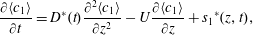 $$\begin{eqnarray}\displaystyle & \displaystyle {\displaystyle \frac{\unicode[STIX]{x2202}\langle c_{1}\rangle }{\unicode[STIX]{x2202}t}}=D^{\ast }(t){\displaystyle \frac{\unicode[STIX]{x2202}^{2}\langle c_{1}\rangle }{\unicode[STIX]{x2202}z^{2}}}-U{\displaystyle \frac{\unicode[STIX]{x2202}\langle c_{1}\rangle }{\unicode[STIX]{x2202}z}}+{s_{1}}^{\ast }(z,t), & \displaystyle\end{eqnarray}$$
 $$\begin{eqnarray}\displaystyle & \displaystyle \text{I.C.1}\quad \langle c_{1}\rangle |_{(z,t=0)}=c_{0}Z_{1}(z). & \displaystyle\end{eqnarray}$$
Problem  $\langle c_{2}\rangle \quad I_{2}:0<t^{\prime }<750~\text{min}$
 $$\begin{eqnarray}\displaystyle & \displaystyle {\displaystyle \frac{\unicode[STIX]{x2202}\langle c_{2}\rangle }{\unicode[STIX]{x2202}t^{\prime }}}=D^{\ast }(t^{\prime }){\displaystyle \frac{\unicode[STIX]{x2202}^{2}\langle c_{2}\rangle }{\unicode[STIX]{x2202}z^{2}}}-U{\displaystyle \frac{\unicode[STIX]{x2202}\langle c_{2}\rangle }{\unicode[STIX]{x2202}z}}+{s_{2}}^{\ast }(z,t^{\prime }), & \displaystyle\end{eqnarray}$$
 $$\begin{eqnarray}\displaystyle & \displaystyle \text{I.C.2}\quad \langle c_{2}\rangle |_{(z,t^{\prime }=0)}=c_{0}Z_{1}(z). & \displaystyle\end{eqnarray}$$
 For the second injection, the time coordinate for the second interval is started at the time  $t^{\prime }=t-T_{1}$, as described in example 1. Without this translation, the second injection would not start with the correct dispersion coefficient, which is $D^{\ast }(t^{\prime }=0)={\mathcal{D}}$, as indicated by (9.2b).
The boundary conditions are identical to those posed in (3.1a)–(3.1e). For reference, the microscale solution to this problem is provided for a number of time points in figure 15. We note that problem  $\langle c_{2}\rangle$ must be put in the time coordinates for which the injection happens at time equal to zero (this was noted in § 7.2) to properly define $D^{\ast }$ and $s^{\ast }$.
Microscale solute distributions in space at selected time points for the problem consisting of two injected pulses; Péclet number is  $Pe=100$. The second pulse is injected at the same location where the first pulse was injected at $t=250~\text{min}$. These images are provided only for visualization of the microscale processes (aspect ratio is 1 : 10 as for figures 6 and 7), and for validation of the macroscale equations by comparison of the directly averaged microscale fields.

We now explore how these two solutions can be superimposed. First, note that the classical principle of superposition (Polyanin Reference Polyanin2000; Olver Reference Olver2014) for linear partial differential equations with time-dependent coefficients requires that the superposition be defined over the same time interval. Thus, problems  $I_{1}$ and $I_{2}$ can be equivalently written as (recalling that for the general problem, the initial condition is represented by $\unicode[STIX]{x1D711}(z)$; cf. (3.1e))
Problem  $\langle c_{1}\rangle \quad I_{1}:0<t<1000~\text{min}$
Interval 1  $\quad 0<t<250~\text{min}$
 $$\begin{eqnarray}\displaystyle & \displaystyle {\displaystyle \frac{\unicode[STIX]{x2202}\langle c_{1}\rangle }{\unicode[STIX]{x2202}t}}=D^{\ast }(t){\displaystyle \frac{\unicode[STIX]{x2202}^{2}\langle c_{1}\rangle }{\unicode[STIX]{x2202}z^{2}}}-U{\displaystyle \frac{\unicode[STIX]{x2202}\langle c_{1}\rangle }{\unicode[STIX]{x2202}z}}+{s_{1}}^{\ast }(z,t), & \displaystyle\end{eqnarray}$$
 $$\begin{eqnarray}\displaystyle & \displaystyle \text{I.C.1}\quad \langle c_{1}\rangle |_{(z,t=0)}=c_{0}Z_{1}(z). & \displaystyle\end{eqnarray}$$
 Interval 2  $\quad 0<t^{\prime }<750~\text{min}$
 $$\begin{eqnarray}\displaystyle & \displaystyle {\displaystyle \frac{\unicode[STIX]{x2202}\langle c_{1}\rangle }{\unicode[STIX]{x2202}t^{\prime }}}=D^{\ast }(t^{\prime }){\displaystyle \frac{\unicode[STIX]{x2202}^{2}\langle c_{1}\rangle }{\unicode[STIX]{x2202}z^{2}}}-U{\displaystyle \frac{\unicode[STIX]{x2202}\langle c_{1}\rangle }{\unicode[STIX]{x2202}z}}+{s_{1}}^{\ast }(z,t^{\prime }), & \displaystyle\end{eqnarray}$$
 $$\begin{eqnarray}\displaystyle & \displaystyle \text{I.C.2}\quad \langle c_{1}\rangle |_{(z,t^{\prime }=0)}=\underbrace{\langle c_{1}\rangle |_{(z,t=T_{1})}}_{\unicode[STIX]{x1D711}_{1}}. & \displaystyle\end{eqnarray}$$
 Problem  $\langle c_{2}\rangle \quad I_{2}:0<t<1000~\text{min}$
Interval 1  $\quad 0<t<250~\text{min}$
 $$\begin{eqnarray}\langle c_{2}\rangle =0.\end{eqnarray}$$
 Interval 2  $\quad 0<t^{\prime }<750~\text{min}$
 $$\begin{eqnarray}\displaystyle & \displaystyle {\displaystyle \frac{\unicode[STIX]{x2202}\langle c_{2}\rangle }{\unicode[STIX]{x2202}t^{\prime }}}=D^{\ast }(t^{\prime }){\displaystyle \frac{\unicode[STIX]{x2202}^{2}\langle c_{2}\rangle }{\unicode[STIX]{x2202}z^{2}}}-U{\displaystyle \frac{\unicode[STIX]{x2202}\langle c_{2}\rangle }{\unicode[STIX]{x2202}z}}+{s_{2}}^{\ast }(z,t^{\prime }), & \displaystyle\end{eqnarray}$$
 $$\begin{eqnarray}\displaystyle & \displaystyle \text{I.C.2}\quad \langle c_{2}\rangle |_{(z,t^{\prime }=0)}=\underbrace{c_{0}Z_{1}(z)}_{\unicode[STIX]{x1D711}_{2}}. & \displaystyle\end{eqnarray}$$
We make the following important notes about the formulation above.
(i) We have divided Problem 1 into two intervals  $0<t<250~\text{min}$ and $250<t<1000~\text{min}$. This is not an arbitrary choice; it is necessary to obtain solutions that involve multiple initial conditions.
(ii) In our formulation, the dispersion coefficient  $D^{\ast }$ does not have to ‘remember’ its prior history. Hence, exactly the same function $D^{\ast }$ is used in both intervals. Being explicit, for the problem for $\langle c_{1}\rangle$ in the first time interval, the dispersion coefficient starts at $D^{\ast }(t=0)={\mathcal{D}}$, and grows as predicted by (7.3). When time is restarted in the second interval, exactly the same behaviour is repeated. The dispersion coefficient for the second time interval starts at $D^{\ast }(t=0)={\mathcal{D}}$, and again grows as predicted by (7.3). During the second time interval, the source function $s_{1}^{\ast }$ automatically accounts for the spreading inherent in the second initial condition. This function is essentially the ‘memory’ in the system, but one that encodes that memory in a local rather than non-local in time representation.
(iii) The source function,  $s^{\ast }$, is linear in the initial condition; this is proved in § A.5. In other words, we have the following decomposition due to linearity:
 $$\begin{eqnarray}s^{\ast }(\unicode[STIX]{x1D711}_{1}+\unicode[STIX]{x1D711}_{2})=s^{\ast }(\unicode[STIX]{x1D711}_{1})+s^{\ast }(\unicode[STIX]{x1D711}_{2}).\end{eqnarray}$$
(iv) These features make the two problems superposable; the two problems can be added to generate one equation that suffices to describe the dispersion process over the two intervals.
9.2.2 Superposition of the two concentrations
We now show how superposition can be accomplished for the problem of two releases of solute at two different times. We begin by defining the superposed concentration  $\langle c\rangle =\langle c_{1}\rangle +\langle c_{2}\rangle$. For the first time interval, the superposition is trivial, noting that $\langle c_{2}\rangle \equiv 0$. Thus, $\langle c\rangle =\langle c_{1}\rangle$. Superposition for the first interval yields
Superposition for interval 1  $\quad 0<t<250~\text{min}$
 $$\begin{eqnarray}\displaystyle & \displaystyle {\displaystyle \frac{\unicode[STIX]{x2202}\langle c\rangle }{\unicode[STIX]{x2202}t}}=D^{\ast }(t){\displaystyle \frac{\unicode[STIX]{x2202}^{2}\langle c\rangle }{\unicode[STIX]{x2202}z^{2}}}-U{\displaystyle \frac{\unicode[STIX]{x2202}\langle c\rangle }{\unicode[STIX]{x2202}z}}+{s_{1}}^{\ast }(z,t), & \displaystyle\end{eqnarray}$$
 $$\begin{eqnarray}\displaystyle & \displaystyle \text{I.C.1}\quad \langle c\rangle |_{(z,t=0)}=c_{0}Z_{1}(z). & \displaystyle\end{eqnarray}$$
 Note that the concentration at the final time  $t=T_{1}=250~\text{min}$, forms the initial condition for $\langle c_{1}\rangle$ during the second interval. For reference, we denote this concentration by $\langle c_{1}\rangle |_{(z,t=T_{1})}$.
Because (9.4d) and (9.4g) are (i) linear, and (ii) defined over the same time interval  $0<t^{\prime }<(T_{f}-T_{1})$, the superposition of these equations is straightforward. Adding (9.4c) and (9.4f) yields
Superposition for interval 2  $\quad 0<t^{\prime }<750~\text{min}$
 $$\begin{eqnarray}{\displaystyle \frac{\unicode[STIX]{x2202}\langle c\rangle }{\unicode[STIX]{x2202}t^{\prime }}}=D^{\ast }(t^{\prime }){\displaystyle \frac{\unicode[STIX]{x2202}^{2}\langle c\rangle }{\unicode[STIX]{x2202}z^{2}}}-U{\displaystyle \frac{\unicode[STIX]{x2202}\langle c\rangle }{\unicode[STIX]{x2202}z}}+s^{\ast }(z,t^{\prime }).\end{eqnarray}$$
 Here, we have used the linearity of the source term:  $s^{\ast }(z,t^{\prime };\unicode[STIX]{x1D711})=s_{1}^{\ast }(z,t^{\prime };\unicode[STIX]{x1D711}_{1})+s_{2}^{\ast }(z,t^{\prime };\unicode[STIX]{x1D711}_{2})$ to generate the single source term field, $s^{\ast }$, for the superposed problem. The initial condition for the second interval is found by adding the final concentration from time interval 1, $\langle c_{1}\rangle |_{(z,t=T_{1})}$, to the initial condition for the second solute release.
 $$\begin{eqnarray}\text{I.C.2}\quad \langle c\rangle |_{(z,t^{\prime }=0)}=\underbrace{\langle c_{1}\rangle |_{(z,t=T_{1})}+c_{0}Z_{1}(z)}_{\unicode[STIX]{x1D711}}.\end{eqnarray}$$
 The Taylor dispersion problem is frequently represented by an equation of the form of (9.4d) and (9.4g), but with  $s_{1}^{\ast }=s_{2}^{\ast }=0$ (cf. Smith Reference Smith1981a). Superposition for this case fails because even if one divides the problem into two time intervals. Upon restarting time (setting $t^{\prime }=0$) for the second interval, the concentrations $\langle c_{1}\rangle$ and $\langle c_{2}\rangle$ are represented by two different linear operators (one for $\langle c_{1}\rangle$ where $D^{\ast }(t)$ begins at $t=T_{1}$, and a second for $\langle c_{2}\rangle$ where $D^{\ast }(t^{\prime })$ begins at $t^{\prime }=0$). In the formulation we provide, $D^{\ast }(t)$ is always given by a single function of time everywhere in the domain; any ‘time history’ associated with multiple injections at different times is accounted for strictly through the source term field, $s^{\ast }$. This avoids the possibility of having $D^{\ast }$ being multi-valued at a single spatial location.
9.2.3 Proof of validity of superposition by direct computation
The superposition of  $\langle c_{1}\rangle$ and $\langle c_{2}\rangle$ is given by (9.6a)–(9.6d). For clarity, we re-emphasize the following regarding the interpretation of these equations:
(i) During the first time interval (
$0<t<T_{1}$) the dispersion coefficient for the time interval starts at $D^{\ast }(t=0)={\mathcal{D}}$, and again grows as predicted by (7.3). This is described by the single transport equation given by (9.6a,b). Because the radial derivative of the initial condition for this interval is zero, we have that $s_{1}^{\ast }(z,t)$ is zero.(ii) For the second time interval, the initial condition is the solution obtained from the end of the first time interval (at
$t=T_{1}$) plus the initial condition representing the second solute release. This is described by the single transport equation given by (9.6c,b).(iii) During the second time interval (
$0<t<T_{1}$) the dispersion coefficient for the time interval starts at $D^{\ast }(t=0)={\mathcal{D}}$, and again grows as predicted by (7.3). Note that the radial derivative of the initial condition for the second time interval is non-zero, thus there is a contribution from the $s^{\ast }$-field for the second time interval.


The initial condition for this problem is similar to that for Problem 1. In fact, the  $s^{\ast }$ field is identical to that for Problem 1, and is computed numerically as described for Problem 1.
The macroscopic concentration field predicted by the upscaled problem statements given by  $I_{1}$ and $I_{2}$. Continuous lines represents the averaged microscale simulation results; points represent the solutions to the upscaled equations given by (9.3a)–(9.3d). The concentration curves are provided as two plots for ease in visualization. Note that the curve in dark blue at $t=250~\text{min}$ represents the macroscale initial condition for problem $I_{2}$ computed by superposition.

In figure 16 we have illustrated the solutions for this problem computed by (i) averaging the microscale numerical solutions directly, and (ii) via the two-step (superposed) macroscale simulation (solving (9.6a)–(9.6d)) as described above. We note that the two solutions are in good agreement, and, in particular, the amount of dispersion predicted by the upscaled model (both before and after the second pulse) is consistent with the averaged microscale data (for which there are no approximations of any kind). There is a slight mismatch in between the two solutions near the peaks for times  $t=100$, 350 and 500 min. Most likely, these errors are associated with the approximations in the upscaled equation, as discussed previously (cf. the peaks for $Pe=100$, Case A in figure 8).
In summary, we have provided two examples that meet the desideratum of Taylor (Reference Taylor1959). For each solution, we find that (i) we can define a sensible notion of superposition for the upscaled equation of the form that we have derived, (ii) the associated dispersion coefficient is always a single-valued function of space and (iii) the source terms are superposable, and they generate a field correction that assures that the proper rate of spreading (or, equivalently, second moment) is achieved. Because the source terms are responsible for correcting the rate of spreading at early times, this function is not imposed on the dispersion coefficient. It is this component of our solution that generates the necessary conditions for the upscaled equation to be superposable.
10 Conclusions
In this study, we were able to address a long-standing problem of early-time behaviour from arbitrary initial conditions. The approach we adopted generates an effective macroscale balance equation that is consistent with the conventional one-dimensional convection–dispersion-type equation. One notable difference is that the formulation presented here also contains an exponentially decaying-in-time source term that represents memory of the initial condition. Because our results were compared with numerical simulations, we were able to compute the errors associated with the approximations made in our development. In short, these approximations are represented by
 $$\begin{eqnarray}\displaystyle & \displaystyle (\text{i})\quad Pe{\displaystyle \frac{a}{L_{0}}}=\boldsymbol{O}(1), & \displaystyle \nonumber\\ \displaystyle & \displaystyle (\text{ii})\quad {\displaystyle \frac{a}{L_{0}}}<1. & \displaystyle \nonumber\end{eqnarray}$$
In addition, the four guidelines that we proposed in the introduction for generating a well-structured dispersion theory were met. Specifically, the dispersion coefficient for Taylor dispersion was shown to be positive, independent of initial conditions, superposable and converges to the classical result at large times. Of these, the most important result was illustrating that the non-conventional source term is necessary to assure that solutions are superposable. This addresses a long-standing problem about maintaining the principle of superposition when a time-dependent dispersion coefficient has been defined.
Acknowledgements
This research was supported by the NSF, project EAR 1521441. The authors would like to thank Professor P. C. Chatwin for valuable feedback and advice on an early draft of this paper (nearly a decade ago) and a copy of the thesis by O’Hara. The authors also thank Professor L. Johns and Dr A. Degance for generously explaining elements of their approach, and for feedback on our efforts. We thank the editor who handled this manuscript and three anonymous reviewers for providing helpful comments that improved the quality and presentation of the manuscript.
Declaration of interests
The authors report no conflict of interest.
Supplementary materials
Supplementary materials are available at https://doi.org/10.1017/jfm.2020.56.
Appendix A. Solutions to the closure problem
A.1 General integral solutions
The balance for the deviations developed in the body of the paper is given by the following set of equations:
 $$\begin{eqnarray}\displaystyle & \displaystyle {\displaystyle \frac{\unicode[STIX]{x2202}\tilde{c}}{\unicode[STIX]{x2202}t}}+\underbrace{\tilde{v}_{z}{\displaystyle \frac{\unicode[STIX]{x2202}\langle c\rangle }{\unicode[STIX]{x2202}z}}}_{source}={\displaystyle \frac{{\mathcal{D}}}{r}}{\displaystyle \frac{\unicode[STIX]{x2202}}{\unicode[STIX]{x2202}r}}\left(r{\displaystyle \frac{\unicode[STIX]{x2202}\tilde{c}}{\unicode[STIX]{x2202}r}}\right)+{\displaystyle \frac{{\mathcal{D}}}{r^{2}}}{\displaystyle \frac{\unicode[STIX]{x2202}^{2}\tilde{c}}{\unicode[STIX]{x2202}\unicode[STIX]{x1D703}^{2}}}+{\mathcal{D}}{\displaystyle \frac{\unicode[STIX]{x2202}^{2}\tilde{c}}{\unicode[STIX]{x2202}z^{2}}}, & \displaystyle\end{eqnarray}$$
 $$\begin{eqnarray}\displaystyle & \displaystyle -{\mathcal{D}}{\displaystyle \frac{\unicode[STIX]{x2202}\tilde{c}}{\unicode[STIX]{x2202}r}}=0,\quad \text{at }r=0,a, & \displaystyle\end{eqnarray}$$
 $$\begin{eqnarray}\displaystyle & \displaystyle \tilde{c}=0,\quad \text{as }z\rightarrow \pm \infty , & \displaystyle\end{eqnarray}$$
 $$\begin{eqnarray}\displaystyle & \displaystyle -{\mathcal{D}}{\displaystyle \frac{\unicode[STIX]{x2202}\tilde{c}}{\unicode[STIX]{x2202}z}}=0,\quad \text{as }z\rightarrow \pm \infty , & \displaystyle\end{eqnarray}$$
 $$\begin{eqnarray}\displaystyle & \displaystyle \tilde{c}(r,\unicode[STIX]{x1D703},z,0)=\underbrace{\tilde{\unicode[STIX]{x1D711}}(r,\unicode[STIX]{x1D703},z)}_{source}, & \displaystyle\end{eqnarray}$$ $\tilde{v}_{z}\unicode[STIX]{x2202}\tilde{c}/\unicode[STIX]{x2202}z-\langle \tilde{v}_{z}\unicode[STIX]{x2202}\tilde{c}/\unicode[STIX]{x2202}z\rangle$ has been neglected with respect to radial diffusion and a Lagrangian frame of coordinates is being used. This problem has exactly two source terms: one due to macroscopic convection and the second one due to the initial condition. The solution of this problem can be carried out by means of integral equations formulations in terms of Green’s functions (Wood & Valdés-Parada Reference Wood and Valdés-Parada2013; Polyanin & Nazaikinskii Reference Polyanin and Nazaikinskii2015) with the associated Green’s function $(G)$ satisfying the following initial and boundary-value problem:
  $$\begin{eqnarray}\displaystyle & \displaystyle {\displaystyle \frac{\unicode[STIX]{x2202}G}{\unicode[STIX]{x2202}t}}={\displaystyle \frac{{\mathcal{D}}}{r}}{\displaystyle \frac{\unicode[STIX]{x2202}}{\unicode[STIX]{x2202}r}}\left(r{\displaystyle \frac{\unicode[STIX]{x2202}G}{\unicode[STIX]{x2202}r}}\right)+{\displaystyle \frac{{\mathcal{D}}}{r^{2}}}{\displaystyle \frac{\unicode[STIX]{x2202}^{2}G}{\unicode[STIX]{x2202}\unicode[STIX]{x1D703}^{2}}}+{\mathcal{D}}{\displaystyle \frac{\unicode[STIX]{x2202}^{2}G}{\unicode[STIX]{x2202}z^{2}}}+\unicode[STIX]{x1D6FF}(r-\unicode[STIX]{x1D70C})\unicode[STIX]{x1D6FF}(\unicode[STIX]{x1D703}-\unicode[STIX]{x1D717})\unicode[STIX]{x1D6FF}(z-\unicode[STIX]{x1D701})\unicode[STIX]{x1D6FF}(t-\unicode[STIX]{x1D70F}),\qquad & \displaystyle\end{eqnarray}$$
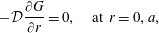 $$\begin{eqnarray}\displaystyle & \displaystyle -{\mathcal{D}}{\displaystyle \frac{\unicode[STIX]{x2202}G}{\unicode[STIX]{x2202}r}}=0,\quad \text{at }r=0,a, & \displaystyle\end{eqnarray}$$
 $$\begin{eqnarray}\displaystyle & \displaystyle G=0,\quad \text{as }z\rightarrow \pm \infty , & \displaystyle\end{eqnarray}$$
 $$\begin{eqnarray}\displaystyle & \displaystyle -{\mathcal{D}}{\displaystyle \frac{\unicode[STIX]{x2202}G}{\unicode[STIX]{x2202}z}}=0,\quad \text{as }z\rightarrow \pm \infty , & \displaystyle\end{eqnarray}$$
 $$\begin{eqnarray}\displaystyle & \displaystyle G=0,\quad t<\unicode[STIX]{x1D70F}. & \displaystyle\end{eqnarray}$$
 $$\begin{eqnarray}G(r,\unicode[STIX]{x1D70C},\unicode[STIX]{x1D703},\unicode[STIX]{x1D717},z,\unicode[STIX]{x1D701},t,\unicode[STIX]{x1D70F})=G_{1}(r,\unicode[STIX]{x1D70C},\unicode[STIX]{x1D703}-\unicode[STIX]{x1D717},t-\unicode[STIX]{x1D70F})G_{2}(z-\unicode[STIX]{x1D701},t-\unicode[STIX]{x1D70F}),\end{eqnarray}$$
 where, for convenience, the solution is expressed in terms of the Green’s functions of unsteady polar  $(G_{1})$ and axial coordinates $(G_{2})$. These Green’s functions are given by
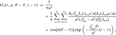 $$\begin{eqnarray}\displaystyle G_{1}(r,\unicode[STIX]{x1D70C},\unicode[STIX]{x1D703}-\unicode[STIX]{x1D717},t-\unicode[STIX]{x1D70F}) & = & \displaystyle {\displaystyle \frac{1}{\unicode[STIX]{x03C0}a^{2}}}\nonumber\\ \displaystyle & & \displaystyle +\,{\displaystyle \frac{1}{\unicode[STIX]{x03C0}}}\mathop{\sum }_{n=0}^{\infty }\mathop{\sum }_{m=1}^{\infty }{\displaystyle \frac{A_{n}\unicode[STIX]{x1D706}_{nm}^{2}\text{J}_{n}(\unicode[STIX]{x1D706}_{nm}r/a)\text{J}_{n}(\unicode[STIX]{x1D706}_{nm}\unicode[STIX]{x1D70C}/a)}{a^{2}(\unicode[STIX]{x1D706}_{nm}^{2}-n^{2})\text{J}_{n}^{2}(\unicode[STIX]{x1D706}_{nm})}}\nonumber\\ \displaystyle & & \displaystyle \times \,\cos [n(\unicode[STIX]{x1D703}-\unicode[STIX]{x1D717})]\exp \left(-{\displaystyle \frac{\unicode[STIX]{x1D706}_{nm}^{2}{\mathcal{D}}}{a^{2}}}(t-\unicode[STIX]{x1D70F})\right),\end{eqnarray}$$
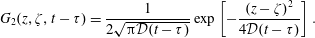 $$\begin{eqnarray}G_{2}(z,\unicode[STIX]{x1D701},t-\unicode[STIX]{x1D70F})={\displaystyle \frac{1}{2\sqrt{\unicode[STIX]{x03C0}{\mathcal{D}}(t-\unicode[STIX]{x1D70F})}}}\exp \left[-{\displaystyle \frac{(z-\unicode[STIX]{x1D701})^{2}}{4{\mathcal{D}}(t-\unicode[STIX]{x1D70F})}}\right].\end{eqnarray}$$
 In (A 4a)  $A_{n}$ is a constant whose value is 1 for $n=0$ and 2 for $n=1,2,\ldots \,$ In addition, $\unicode[STIX]{x1D706}_{nm}$ are the positive roots of the transcendental equation $\text{J}_{n}^{\prime }(\unicode[STIX]{x1D706}_{nm})=0$. The solution of the problem given in (A 1e) can be obtained by using the unsteady version of Green’s formula and the resulting expression can be written in the form given in (5.11). Direct substitution of this result into the unclosed macroscale balance equation yields the closed but non-local model given in (6.1).
A.2 Localized solutions
The relative advantages and disadvantages of non-local formulations have been discussed in the body of the paper. Regardless, we are ultimately interested in finding analytical solutions for the effective parameters that arise from averaging, so a localized form is desirable. Recall, this is valid when there is separation between the characteristic space and time scales for the microscale and macroscale variables, i.e.
 $$\begin{eqnarray}\displaystyle & a\ll L_{0}, & \displaystyle\end{eqnarray}$$
 $$\begin{eqnarray}\displaystyle & t^{\ast }\ll T^{\ast }, & \displaystyle\end{eqnarray}$$ $L_{0}$ is a measure of the size of the initial configuration in the longitudinal direction, $t^{\ast }$ is the characteristic time scale for the microscale processes and $T^{\ast }$ is the characteristic time scale for the macroscale processes.
 The length scale constraint is fairly clear in that it is expressed in terms of physical properties of the system. For the time scales, the restriction is less clear. We can attempt to (very roughly) characterize these time scales as follows. There are two reasonable time scales associated with the microscale balance given by (A 1a). First, the convection term involved in the material time derivative has a time scale that would be estimated by  $T^{\ast }=\boldsymbol{O}(L/U)$. The diffusive time scale in the radial direction is estimated by $t^{\ast }=\boldsymbol{O}(a^{2}/(4{\mathcal{D}}))$. If we assume that $Pe_{T}\leqslant \boldsymbol{O}(1)$, then the diffusive time scale can be used for estimates. For the macroscale equation, (6.6a), estimates are complicated somewhat by the fact that the length scale of interest, $L$, is the longitudinal size of the solution as it spreads. Noting that we are attempting to generate estimates for the length scale associated with $\unicode[STIX]{x2202}\langle c\rangle /\unicode[STIX]{x2202}z$ in the convolutions given by (5.11), we can neglect the convection term (since we are in a moving coordinate system). The time scale can be estimated from the dispersive time scale, which we can think of as containing an initial time scale plus a transient time scale. In other words, we are making the estimate
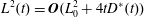 $$\begin{eqnarray}L^{2}(t)=\boldsymbol{O}(L_{0}^{2}+4tD^{\ast }(t))\end{eqnarray}$$
from which we generate the time scale
 $$\begin{eqnarray}T^{\ast }=\boldsymbol{O}\left({\displaystyle \frac{L_{0}^{2}}{D^{\ast }(0)}}+{\displaystyle \frac{4D^{\ast }(t)t}{D^{\ast }(0)}}\right)=\boldsymbol{O}\left({\displaystyle \frac{L_{0}^{2}}{{\mathcal{D}}}}+4t\right).\end{eqnarray}$$
 Recalling  $t^{\ast }=\boldsymbol{O}(a^{2}/(4{\mathcal{D}}))$, it is clear that the constraint $t^{\ast }\ll T^{\ast }$ is automatically met when $a\ll L_{0}$. Therefore, the single length scale constraint appears to be sufficient to justify the analysis, and this has been adopted in the body of the paper. We note that an alternate analysis of approximations of this sort is available in Mercer & Roberts (Reference Mercer and Roberts1990, appendix A), where the analysis is carried out in Fourier space in the context of a centre manifold theory approach to upscaling.
Additional details (and refinements about specific metrics for the time and length scales) for this approximation can be found in Wood & Valdés-Parada (Reference Wood and Valdés-Parada2013). Regardless, exact conditions for when this approximation can be imposed are difficult to define; instead, we opt for the approach here of making the assumption that this approximation holds, and then examining the fidelity of the results. We do note that the removal of the axial derivative of the concentration is consistent with the second-order truncation presented by Gill & Sankarasubramanian (Reference Gill and Sankarasubramanian1970). The work of Gill & Sankarasubramanian (Reference Gill and Sankarasubramanian1970) suggests that the higher-order terms are much smaller than the second-order terms, which provides an independent validation of the approximation that we have employed.
A.3 Analytical solutions for the $b$-field

Assuming that the constraints allowing a local solution are valid, we can extract the axial derivative of the average concentration from the second integral in (5.11), we set
 $$\begin{eqnarray}\displaystyle b(r,\unicode[STIX]{x1D703},z,t) & = & \displaystyle -\int _{\unicode[STIX]{x1D70F}=0}^{\unicode[STIX]{x1D70F}=t}\int _{\unicode[STIX]{x1D701}=-\infty }^{\unicode[STIX]{x1D701}=\infty }\int _{\unicode[STIX]{x1D717}=0}^{\unicode[STIX]{x1D717}=2\unicode[STIX]{x03C0}}\int _{\unicode[STIX]{x1D70C}=0}^{\unicode[STIX]{x1D70C}=a}G(r,\unicode[STIX]{x1D70C},\unicode[STIX]{x1D703},\unicode[STIX]{x1D717},z,\unicode[STIX]{x1D701},t-\unicode[STIX]{x1D70F})\tilde{v}_{z}(\unicode[STIX]{x1D70C})\unicode[STIX]{x1D70C}\,\text{d}\unicode[STIX]{x1D70C}\,\text{d}\unicode[STIX]{x1D717}\,\text{d}\unicode[STIX]{x1D701}\,\text{d}\unicode[STIX]{x1D70F}\nonumber\\ \displaystyle & = & \displaystyle -\int _{\unicode[STIX]{x1D70F}=0}^{\unicode[STIX]{x1D70F}=t}\int _{\unicode[STIX]{x1D717}=0}^{\unicode[STIX]{x1D717}=2\unicode[STIX]{x03C0}}\int _{\unicode[STIX]{x1D70C}=0}^{\unicode[STIX]{x1D70C}=a}G_{1}(r,\unicode[STIX]{x1D70C},\unicode[STIX]{x1D703}-\unicode[STIX]{x1D717},t-\unicode[STIX]{x1D70F})\tilde{v}_{z}(\unicode[STIX]{x1D70C})\unicode[STIX]{x1D70C}\,\text{d}\unicode[STIX]{x1D70C}\,\text{d}\unicode[STIX]{x1D717}\nonumber\\ \displaystyle & & \displaystyle \times \,\int _{\unicode[STIX]{x1D701}=-\infty }^{\unicode[STIX]{x1D701}=\infty }G_{2}(z-\unicode[STIX]{x1D701},t-\unicode[STIX]{x1D70F})\,\text{d}\unicode[STIX]{x1D701}\,\text{d}\unicode[STIX]{x1D70F}.\end{eqnarray}$$
Note, we can make use of the identity
 $$\begin{eqnarray}\int _{\unicode[STIX]{x1D701}=-\infty }^{\unicode[STIX]{x1D701}=\infty }G_{2}(z-\unicode[STIX]{x1D701},t-\unicode[STIX]{x1D70F})\,\text{d}\unicode[STIX]{x1D701}=1,\quad (t-\unicode[STIX]{x1D70F}\neq 0).\end{eqnarray}$$
 It is clear from these results that the  $b$-field is entirely independent of the particular initial condition adopted. Also, because of symmetry, the velocity deviations do not depend on the angular direction, $\unicode[STIX]{x1D703}$ or longitudinal coordinate, $z$. Direct integration leads to a result that is only a function of $r$ and $t$
$t$
 $$\begin{eqnarray}b(r,t)={\displaystyle \frac{1}{4}}{\displaystyle \frac{Ua^{2}}{{\mathcal{D}}}}\left({\displaystyle \frac{r^{2}}{a^{2}}}-{\displaystyle \frac{r^{4}}{2a^{4}}}-{\displaystyle \frac{1}{3}}\right)+{\displaystyle \frac{2Ua^{2}}{{\mathcal{D}}}}\mathop{\sum }_{n=1}^{\infty }{\displaystyle \frac{\text{J}_{3}(\unicode[STIX]{x1D706}_{n})\text{J}_{0}\left(\unicode[STIX]{x1D706}_{n}{\displaystyle \frac{r}{a}}\right)}{\unicode[STIX]{x1D706}_{n}^{3}\text{J}_{0}^{2}(\unicode[STIX]{x1D706}_{n})}}\exp \left(-\unicode[STIX]{x1D706}_{n}^{2}{\displaystyle \frac{{\mathcal{D}}}{a^{2}}}t\right).\end{eqnarray}$$
A simplification has been used here to decompose the series into the steady and transient parts, noting
 $$\begin{eqnarray}\mathop{\sum }_{n=1}^{\infty }{\displaystyle \frac{\text{J}_{3}(\unicode[STIX]{x1D706}_{n})\text{J}_{0}(\unicode[STIX]{x1D706}_{n}{\textstyle \frac{r}{a}})}{\unicode[STIX]{x1D706}_{n}^{3}\text{J}_{0}^{2}(\unicode[STIX]{x1D706}_{n})}}=-{\displaystyle \frac{1}{8}}\left({\displaystyle \frac{r^{2}}{a^{2}}}-{\displaystyle \frac{r^{4}}{2a^{4}}}-{\displaystyle \frac{1}{3}}\right).\end{eqnarray}$$
 It is easy to verify that  $\langle b\rangle =0$. Similarly, as $t\rightarrow \infty$, we find
 $$\begin{eqnarray}\displaystyle -\langle \tilde{v}_{z}b\rangle |_{t\rightarrow \infty } & = & \displaystyle -{\displaystyle \frac{1}{2}}{\displaystyle \frac{U^{2}a^{2}}{{\mathcal{D}}}}\left\langle \left({\displaystyle \frac{r^{2}}{a^{2}}}-{\displaystyle \frac{r^{4}}{2a^{4}}}-{\displaystyle \frac{1}{3}}\right)\left({\displaystyle \frac{1}{2}}-{\displaystyle \frac{r^{2}}{a^{2}}}\right)\right\rangle \nonumber\\ \displaystyle & = & \displaystyle {\displaystyle \frac{U^{2}a^{2}}{48{\mathcal{D}}}},\end{eqnarray}$$
as expected.
A.4 Analytical solutions for the $\unicode[STIX]{x1D6F7}$-field

Following an analysis analogous to that for the  $b$-field, we define the following functional, $\unicode[STIX]{x1D6F7}(\tilde{\unicode[STIX]{x1D711}})$:
 $$\begin{eqnarray}\unicode[STIX]{x1D6F7}(r,\unicode[STIX]{x1D703},z,t;\tilde{\unicode[STIX]{x1D711}})=\int _{\unicode[STIX]{x1D701}=-\infty }^{\unicode[STIX]{x1D701}=\infty }\int _{\unicode[STIX]{x1D717}=0}^{\unicode[STIX]{x1D717}=2\unicode[STIX]{x03C0}}\int _{\unicode[STIX]{x1D70C}=0}^{\unicode[STIX]{x1D70C}=a}G(r,\unicode[STIX]{x1D70C},\unicode[STIX]{x1D703},\unicode[STIX]{x1D717},z,\unicode[STIX]{x1D701},t)\tilde{\unicode[STIX]{x1D711}}(\unicode[STIX]{x1D70C},\unicode[STIX]{x1D717},\unicode[STIX]{x1D701})\unicode[STIX]{x1D70C}\,\text{d}\unicode[STIX]{x1D70C}\,\text{d}\unicode[STIX]{x1D717}\,\text{d}\unicode[STIX]{x1D701}.\end{eqnarray}$$
 Evidently, in order to draw a specific expression for this closure variable it is necessary to provide a particular initial condition,  $\tilde{\unicode[STIX]{x1D711}}$. Substituting the Green’s function $G$ into (A 13), and rearranging, we recover the result given in (7.7) of the main text, which is applicable to a general initial condition
 $$\begin{eqnarray}\unicode[STIX]{x1D6F7}(r,\unicode[STIX]{x1D703},z,t)=B_{0,0}(z,t)+\mathop{\sum }_{n=0}^{\infty }\mathop{\sum }_{m=1}^{\infty }B_{n,m}(\unicode[STIX]{x1D703},z,t)\text{J}_{n}\left({\displaystyle \frac{\unicode[STIX]{x1D706}_{nm}r}{a}}\right)\exp \left(-{\displaystyle \frac{\unicode[STIX]{x1D706}_{nm}^{2}{\mathcal{D}}}{a^{2}}}t\right),\end{eqnarray}$$
 where the functions  $B_{0,0}(z,t)$ and $B_{n,m}(\unicode[STIX]{x1D703},z,t)$, are defined by
 $$\begin{eqnarray}B_{0,0}(z,t)={\displaystyle \frac{1}{\unicode[STIX]{x03C0}a^{2}}}\int _{\unicode[STIX]{x1D701}=-\infty }^{\unicode[STIX]{x1D701}=\infty }G_{2}(z,\unicode[STIX]{x1D701},t)\int _{\unicode[STIX]{x1D717}=0}^{\unicode[STIX]{x1D717}=2\unicode[STIX]{x03C0}}\int _{\unicode[STIX]{x1D70C}=0}^{\unicode[STIX]{x1D70C}=a}\tilde{\unicode[STIX]{x1D711}}(\unicode[STIX]{x1D70C},\unicode[STIX]{x1D717},\unicode[STIX]{x1D701})\unicode[STIX]{x1D70C}\,\text{d}\unicode[STIX]{x1D70C}\,\text{d}\unicode[STIX]{x1D717}\,\text{d}\unicode[STIX]{x1D701},\end{eqnarray}$$
 $$\begin{eqnarray}\displaystyle B_{n,m}(\unicode[STIX]{x1D703},z,t) & = & \displaystyle {\displaystyle \frac{A_{n}\unicode[STIX]{x1D706}_{nm}^{2}}{\unicode[STIX]{x03C0}a^{2}(\unicode[STIX]{x1D706}_{nm}^{2}-n^{2})\text{J}_{n}^{2}(\unicode[STIX]{x1D706}_{nm})}}\int _{\unicode[STIX]{x1D701}=-\infty }^{\unicode[STIX]{x1D701}=\infty }G_{2}(z,\unicode[STIX]{x1D701},t)\int _{\unicode[STIX]{x1D717}=0}^{\unicode[STIX]{x1D717}=2\unicode[STIX]{x03C0}}\cos [n(\unicode[STIX]{x1D703}-\unicode[STIX]{x1D717})]\nonumber\\ \displaystyle & & \displaystyle \times \,\int _{\unicode[STIX]{x1D70C}=0}^{\unicode[STIX]{x1D70C}=a}\text{J}_{n}\left(\unicode[STIX]{x1D706}_{nm}{\displaystyle \frac{\unicode[STIX]{x1D70C}}{a}}\right)\tilde{\unicode[STIX]{x1D711}}(\unicode[STIX]{x1D70C},\unicode[STIX]{x1D717},\unicode[STIX]{x1D701})\unicode[STIX]{x1D70C}\,\text{d}\unicode[STIX]{x1D70C}\,\text{d}\unicode[STIX]{x1D717}\,\text{d}\unicode[STIX]{x1D701}.\end{eqnarray}$$
 In principle, this expression (combined with (A 15a) and (A 15b)) provides the integral solution for any initial condition. Regardless of the particular initial condition chosen, note that  $\unicode[STIX]{x1D6F7}$ is linear in the initial condition function, i.e.
 $$\begin{eqnarray}\unicode[STIX]{x1D711}=\langle \unicode[STIX]{x1D711}\rangle +\tilde{\unicode[STIX]{x1D711}},\end{eqnarray}$$
 hence, multiplying the initial condition by a constant  $K_{1}$ yields
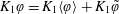 $$\begin{eqnarray}K_{1}\unicode[STIX]{x1D711}=K_{1}\langle \unicode[STIX]{x1D711}\rangle +K_{1}\tilde{\unicode[STIX]{x1D711}}\end{eqnarray}$$
or
 $$\begin{eqnarray}K_{1}\unicode[STIX]{x1D711}\Rightarrow K_{1}\tilde{\unicode[STIX]{x1D711}}.\end{eqnarray}$$
The linearity in the initial condition is then established by
 $$\begin{eqnarray}\unicode[STIX]{x1D6F7}(K_{1}\tilde{\unicode[STIX]{x1D711}_{1}}+K_{2}\tilde{\unicode[STIX]{x1D711}_{2}})=K_{1}\unicode[STIX]{x1D6F7}(\unicode[STIX]{x1D711}_{1})+K_{1}\unicode[STIX]{x1D6F7}(\unicode[STIX]{x1D711}_{2}),\end{eqnarray}$$
as determined from (A 13).
As mentioned in the main body of the paper, we have found (non-trivial) particular solutions in analytical form (i.e. no unresolved integrations remain, and the result is given as a series expression) only for the case of  $\unicode[STIX]{x1D703}$-symmetric initial conditions. For the case of $\unicode[STIX]{x1D703}$-symmetric initial conditions, the resulting expression for the closure variable $\unicode[STIX]{x1D6F7}$ simplifies to
 $$\begin{eqnarray}\unicode[STIX]{x1D6F7}(r,z,t)=\mathop{\sum }_{n=1}^{\infty }B_{n}(z,t)\text{J}_{0}\left(\unicode[STIX]{x1D706}_{n}{\displaystyle \frac{r}{a}}\right)\exp \left(-\unicode[STIX]{x1D706}_{n}^{2}{\displaystyle \frac{{\mathcal{D}}}{a^{2}}}t\right),\end{eqnarray}$$
where  $B_{n}(z,t)$ is defined by
 $$\begin{eqnarray}B_{n}(z,t)={\displaystyle \frac{2}{a^{2}\text{J}_{0}^{2}(\unicode[STIX]{x1D706}_{n})}}\int _{\unicode[STIX]{x1D701}=-\infty }^{\unicode[STIX]{x1D701}=\infty }G_{2}(z-\unicode[STIX]{x1D701},t)\int _{\unicode[STIX]{x1D70C}=0}^{\unicode[STIX]{x1D70C}=a}\tilde{\unicode[STIX]{x1D711}}(\unicode[STIX]{x1D70C},\unicode[STIX]{x1D701})\text{J}_{0}\left(\unicode[STIX]{x1D706}_{n}{\displaystyle \frac{\unicode[STIX]{x1D70C}}{a}}\right)\unicode[STIX]{x1D70C}\,\text{d}\unicode[STIX]{x1D70C}\,\text{d}\unicode[STIX]{x1D701}.\end{eqnarray}$$
 Note that in these results  $\unicode[STIX]{x1D6F7}$ is a time-decaying function that depends on $t$,
$t$,  $r$ and $z$. The dependence on the axial direction arises from the initial condition. Furthermore, we note that if the initial condition is chosen to be independent of $r$, the consequence is that $B_{n}(z,0)=0$ and therefore $\unicode[STIX]{x1D6F7}=0$. As a final note, because $\langle \text{J}_{0}(\unicode[STIX]{x1D706}_{n}(r/a))\rangle \equiv 0$, we have that $\langle \unicode[STIX]{x1D6F7}\rangle \equiv 0$ for all admissible initial conditions.
As a final note about the localized solutions, we note that with the developments above the concentration deviations specified by (5.11) can be put in the local formulation
 $$\begin{eqnarray}\tilde{c}(r,\unicode[STIX]{x1D703},z,t)=b(r,t)\left.{\displaystyle \frac{\unicode[STIX]{x2202}\langle c\rangle }{\unicode[STIX]{x2202}z}}\right|_{(z,t)}+\unicode[STIX]{x1D6F7}(r,\unicode[STIX]{x1D703},z,t).\end{eqnarray}$$
The local macroscale balance equation is easily found to take the form given in (6.6a) of the main body of the paper.
A.5 Analytical solutions for the effective coefficients
Recall that the two effective parameters arising in the macroscale equation are
 $$\begin{eqnarray}\displaystyle & \displaystyle D^{\ast }(t)={\mathcal{D}}-\langle \tilde{v}_{z}b\rangle , & \displaystyle\end{eqnarray}$$
 $$\begin{eqnarray}\displaystyle & \displaystyle s^{\ast }(z,t)=-\left\langle \tilde{v}_{z}{\displaystyle \frac{\unicode[STIX]{x2202}\unicode[STIX]{x1D6F7}}{\unicode[STIX]{x2202}z}}\right\rangle . & \displaystyle\end{eqnarray}$$ $\unicode[STIX]{x1D6F7}$ is a linear functional of the initial condition $\tilde{\unicode[STIX]{x1D711}}$ (or, equivalently, $\unicode[STIX]{x1D711}$; see § A.4), then so is $s^{\ast }(\tilde{\unicode[STIX]{x1D711}})$. This is easy to check by direct substitution
  $$\begin{eqnarray}\displaystyle s^{\ast }(K_{1}\tilde{\unicode[STIX]{x1D711}_{1}}+K_{2}\tilde{\unicode[STIX]{x1D711}_{2}}) & = & \displaystyle -\left\langle \tilde{v}_{z}{\displaystyle \frac{\unicode[STIX]{x2202}\unicode[STIX]{x1D6F7}(K_{1}\tilde{\unicode[STIX]{x1D711}_{1}}+K_{2}\tilde{\unicode[STIX]{x1D711}_{2}})}{\unicode[STIX]{x2202}z}}\right\rangle \nonumber\\ \displaystyle & = & \displaystyle -K_{1}\left\langle \tilde{v}_{z}{\displaystyle \frac{\unicode[STIX]{x2202}\unicode[STIX]{x1D6F7}(\tilde{\unicode[STIX]{x1D711}_{1}})}{\unicode[STIX]{x2202}z}}\right\rangle -K_{2}\left\langle \tilde{v}_{z}{\displaystyle \frac{\unicode[STIX]{x2202}\unicode[STIX]{x1D6F7}(\tilde{\unicode[STIX]{x1D711}_{2}})}{\unicode[STIX]{x2202}z}}\right\rangle \nonumber\\ \displaystyle & = & \displaystyle K_{1}s^{\ast }(\tilde{\unicode[STIX]{x1D711}_{1}})+K_{2}s^{\ast }(\tilde{\unicode[STIX]{x1D711}_{2}})\end{eqnarray}$$
or, equivalently, this linearity can be expressed in terms of the original initial conditions (see § A.4)
 $$\begin{eqnarray}s^{\ast }(K_{1}\unicode[STIX]{x1D711}_{1}+K_{2}\unicode[STIX]{x1D711}_{2})=K_{1}s^{\ast }(\unicode[STIX]{x1D711}_{1})+K_{2}s^{\ast }(\unicode[STIX]{x1D711}_{2}).\end{eqnarray}$$
 To compute  $D^{\ast }$, it is helpful to note the following
 $$\begin{eqnarray}\left\langle \tilde{v}_{z}\text{J}_{0}\left(\unicode[STIX]{x1D706}_{n}{\displaystyle \frac{r}{a}}\right)\right\rangle ={\displaystyle \frac{2U}{\unicode[STIX]{x1D706}_{n}}}\text{J}_{3}(\unicode[STIX]{x1D706}_{n}).\end{eqnarray}$$
Using this average and the result of (A 12), the value of the effective dispersion coefficient is found to be
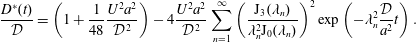 $$\begin{eqnarray}{\displaystyle \frac{D^{\ast }(t)}{{\mathcal{D}}}}=\left(1+{\displaystyle \frac{1}{48}}{\displaystyle \frac{U^{2}a^{2}}{{\mathcal{D}}^{2}}}\right)-4{\displaystyle \frac{U^{2}a^{2}}{{\mathcal{D}}^{2}}}\mathop{\sum }_{n=1}^{\infty }\left({\displaystyle \frac{\text{J}_{3}(\unicode[STIX]{x1D706}_{n})}{\unicode[STIX]{x1D706}_{n}^{2}\text{J}_{0}(\unicode[STIX]{x1D706}_{n})}}\right)^{2}\exp \left(-\unicode[STIX]{x1D706}_{n}^{2}{\displaystyle \frac{{\mathcal{D}}}{a^{2}}}t\right).\end{eqnarray}$$
 Note that, at  $t=0$, the infinite series can be verified to be absolutely convergent. We also note that
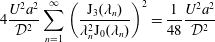 $$\begin{eqnarray}4{\displaystyle \frac{U^{2}a^{2}}{{\mathcal{D}}^{2}}}\mathop{\sum }_{n=1}^{\infty }\left({\displaystyle \frac{\text{J}_{3}(\unicode[STIX]{x1D706}_{n})}{\unicode[STIX]{x1D706}_{n}^{2}\text{J}_{0}(\unicode[STIX]{x1D706}_{n})}}\right)^{2}={\displaystyle \frac{1}{48}}{\displaystyle \frac{U^{2}a^{2}}{{\mathcal{D}}^{2}}}\end{eqnarray}$$
 so that at the initial time we have that  $D^{\ast }(t)={\mathcal{D}}$; clearly, this series must be a monotonically increasing function of time. This also serves to show that the effective hydrodynamic diffusion coefficient is positive for all possible values of time. Equation (A 27) is equivalent to equation (19) in Gill & Sankarasubramanian (Reference Gill and Sankarasubramanian1970) (the comparison of solutions requires the identity $4/\unicode[STIX]{x1D706}_{n}\text{J}_{2}(\unicode[STIX]{x1D706}_{n})=\text{J}_{3}(\unicode[STIX]{x1D706}_{n})$).
For computing  $s^{\ast }$, (A 23b) is reworked by gathering the functions of the radial position into the averaging operator; the resulting equation is given in (7.9) of the main text. For the case in which the initial condition is $\unicode[STIX]{x1D703}$-independent, this result simplifies to
 $$\begin{eqnarray}s^{\ast }(z,t)=-\mathop{\sum }_{n=1}^{n=\infty }\left.{\displaystyle \frac{\unicode[STIX]{x2202}B_{n}}{\unicode[STIX]{x2202}z}}\right|_{(z,t)}\left\langle \tilde{v}_{z}\text{J}_{0}\left(\unicode[STIX]{x1D706}_{n}{\displaystyle \frac{r}{a}}\right)\right\rangle \exp \left(-\unicode[STIX]{x1D706}_{n}^{2}{\displaystyle \frac{{\mathcal{D}}}{a^{2}}}t\right),\end{eqnarray}$$
which can be further reduced, by taking into account the result given in (A 26)
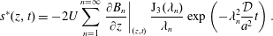 $$\begin{eqnarray}s^{\ast }(z,t)=-2U\mathop{\sum }_{n=1}^{n=\infty }\left.{\displaystyle \frac{\unicode[STIX]{x2202}B_{n}}{\unicode[STIX]{x2202}z}}\right|_{(z,t)}{\displaystyle \frac{\text{J}_{3}(\unicode[STIX]{x1D706}_{n})}{\unicode[STIX]{x1D706}_{n}}}\exp \left(-\unicode[STIX]{x1D706}_{n}^{2}{\displaystyle \frac{{\mathcal{D}}}{a^{2}}}t\right).\end{eqnarray}$$
Note that the source term, when integrated over the entire domain, is identically zero. This is straightforward to show. First note
 $$\begin{eqnarray}\left.\int _{z=-\infty }^{z=\infty }{\displaystyle \frac{\unicode[STIX]{x2202}\unicode[STIX]{x1D6F7}}{\unicode[STIX]{x2202}z}}\,\text{d}z=\unicode[STIX]{x1D6F7}(z)\right|_{-\infty }^{\infty }=0.\end{eqnarray}$$
 Then, we can integrate both sides of  $s^{\ast }$ to yield
 $$\begin{eqnarray}\int _{z=-\infty }^{z=\infty }s^{\ast }(z)\,\text{d}z=-\left\langle \tilde{v}_{z}(r)\int _{z=-\infty }^{z=\infty }{\displaystyle \frac{\unicode[STIX]{x2202}\unicode[STIX]{x1D6F7}}{\unicode[STIX]{x2202}z}}\,\text{d}z\right\rangle =0.\end{eqnarray}$$
 The condition that the integral of  $s^{\ast }$ taken over the entire domain be zero is crucial to the problem. Without this condition, the macroscale balance given by (6.6a) would have no well-defined steady-state solution.
A.6 Numerical solutions for $\unicode[STIX]{x1D6F7}$

In § 9 of the body of the paper, a method for numerically computing  $\unicode[STIX]{x1D6F7}$ is needed for examining the problem of superposition. In general, a numerical method for determining the closure variables (and, hence, the effective parameters) can be found by substituting the solution form given by (A 22) into the general statement for the deviation balance ((A 1a)–(A 1e)). The result is the following two initial and boundary-value problems that can be solved numerically for the closure variables $b$ and $\unicode[STIX]{x1D6F7}$. Because we do not need to solve the balance equation for $b$ numerically at all for this problem, we present only the result for computing the solution for $\unicode[STIX]{x1D6F7}$ numerically. In summary, the value of the $\unicode[STIX]{x1D6F7}$ field can be found by solving the following initial and boundary-value problem:
 $$\begin{eqnarray}\displaystyle & \displaystyle {\displaystyle \frac{\unicode[STIX]{x2202}\unicode[STIX]{x1D6F7}}{\unicode[STIX]{x2202}t}}={\displaystyle \frac{{\mathcal{D}}}{r}}{\displaystyle \frac{\unicode[STIX]{x2202}}{\unicode[STIX]{x2202}r}}\left(r{\displaystyle \frac{\unicode[STIX]{x2202}\unicode[STIX]{x1D6F7}}{\unicode[STIX]{x2202}r}}\right)+{\mathcal{D}}{\displaystyle \frac{\unicode[STIX]{x2202}^{2}\unicode[STIX]{x1D6F7}}{\unicode[STIX]{x2202}z^{2}}}, & \displaystyle\end{eqnarray}$$
 $$\begin{eqnarray}\displaystyle & \displaystyle \left.{\displaystyle \frac{\unicode[STIX]{x2202}\unicode[STIX]{x1D6F7}}{\unicode[STIX]{x2202}r}}\right|_{(r,\unicode[STIX]{x1D703},z,t)}=0,\quad r=0,a, & \displaystyle\end{eqnarray}$$
 $$\begin{eqnarray}\displaystyle & \displaystyle \unicode[STIX]{x1D6F7}(r,\unicode[STIX]{x1D703},z,t)=0,\quad \text{for }z\rightarrow \pm \infty , & \displaystyle\end{eqnarray}$$
 $$\begin{eqnarray}\displaystyle & \displaystyle \left.-{\mathcal{D}}{\displaystyle \frac{\unicode[STIX]{x2202}\unicode[STIX]{x1D6F7}}{\unicode[STIX]{x2202}z}}\right|_{(r,\unicode[STIX]{x1D703},z,t)}=0,\quad \text{for }z\rightarrow \pm \infty , & \displaystyle\end{eqnarray}$$
 $$\begin{eqnarray}\displaystyle & \displaystyle \unicode[STIX]{x1D6F7}(r,\unicode[STIX]{x1D703},z,0)=\tilde{\unicode[STIX]{x1D711}}(r,z). & \displaystyle\end{eqnarray}$$
Appendix B. Particular solution for $s^{\ast }$

As detailed above, the resulting expression for  $s^{\ast }$ depends on the particular type of initial condition in the system by means of $B_{n}(z,0)$, as expressed in (A 21). In this section, an explicit form for $B_{n}(z,0)$ (and consequently for $s^{\ast }$) is obtained by considering the case where the initial condition for the concentration of the solute is separable. As a matter of convenience, let the initial condition for the solute concentration be the superposition of two spatial functions.
To start, we impose the following structure on the initial condition, which summarizes the three case studies of interest here as explained in § 7.3 of the main text,
 $$\begin{eqnarray}\unicode[STIX]{x1D711}(r,z)=R_{1}(r)Z_{1}(z)+R_{2}(r)Z_{2}(z),\end{eqnarray}$$
 where  $R_{1}$ and $R_{2}$ are dimensionless piece-wise continuous functions of the radial position that will be specified later. Averaging then yields
 $$\begin{eqnarray}\langle \unicode[STIX]{x1D711}\rangle (z)=\langle R_{1}\rangle Z_{1}(z)+\langle R_{2}\rangle Z_{2}(z).\end{eqnarray}$$
When subtracted from (B 1), the result gives rise to the following expression for the initial condition of the spatial deviations:
 $$\begin{eqnarray}\tilde{\unicode[STIX]{x1D711}}(r,z)=\tilde{R}_{1}(r)Z_{1}(z)+\tilde{R}_{2}(r)Z_{2}(z).\end{eqnarray}$$
For the particular functions adopted here, we consider a linear function in the radial direction, and a Gaussian type function in the longitudinal direction. Thus we have
 $$\begin{eqnarray}\displaystyle & \displaystyle Z_{1}(z)=c_{0}\unicode[STIX]{x1D6FC}_{1}\exp \left(-{\displaystyle \frac{(z-\unicode[STIX]{x1D6FD}_{1})^{2}}{\unicode[STIX]{x1D70E}_{1}^{2}}}\right), & \displaystyle\end{eqnarray}$$
 $$\begin{eqnarray}\displaystyle & \displaystyle Z_{2}(z)=c_{0}\unicode[STIX]{x1D6FC}_{2}\exp \left(-{\displaystyle \frac{(z-\unicode[STIX]{x1D6FD}_{2})^{2}}{\unicode[STIX]{x1D70E}_{2}^{2}}}\right). & \displaystyle\end{eqnarray}$$ $\unicode[STIX]{x1D6FC}_{1}$, and $\unicode[STIX]{x1D6FC}_{2}$ control the magnitude of the function, $\unicode[STIX]{x1D70E}_{1}$ and $\unicode[STIX]{x1D70E}_{2}$ control the width and $\unicode[STIX]{x1D6FD}_{1}$ and $\unicode[STIX]{x1D6FD}_{2}$ control the displacement along the $z$-axis.
B.1 Linear function in radial distributions
For the radial functions  $R_{1}$ and $R_{2}$, we use the simple linear functions
 $$\begin{eqnarray}\displaystyle & \displaystyle R_{1}(r)=1-{\displaystyle \frac{r}{a}}, & \displaystyle\end{eqnarray}$$
 $$\begin{eqnarray}\displaystyle & \displaystyle R_{2}(r)={\displaystyle \frac{r}{a}}. & \displaystyle\end{eqnarray}$$
 $$\begin{eqnarray}\displaystyle & \displaystyle \tilde{R}_{1}(r)={\displaystyle \frac{2}{3}}-{\displaystyle \frac{r}{a}}, & \displaystyle\end{eqnarray}$$
 $$\begin{eqnarray}\displaystyle & \displaystyle \tilde{R}_{2}(r)={\displaystyle \frac{r}{a}}-{\displaystyle \frac{2}{3}}. & \displaystyle\end{eqnarray}$$
 $$\begin{eqnarray}\tilde{\unicode[STIX]{x1D711}}(z,r)=\left({\displaystyle \frac{2}{3}}-{\displaystyle \frac{r}{a}}\right)c_{0}\unicode[STIX]{x1D6FC}_{1}\exp \left(-{\displaystyle \frac{(z-\unicode[STIX]{x1D6FD}_{1})^{2}}{\unicode[STIX]{x1D70E}_{1}^{2}}}\right)+\left({\displaystyle \frac{r}{a}}-{\displaystyle \frac{2}{3}}\right)c_{0}\unicode[STIX]{x1D6FC}_{2}\exp \left(-{\displaystyle \frac{(z-\unicode[STIX]{x1D6FD}_{2})^{2}}{\unicode[STIX]{x1D70E}_{2}^{2}}}\right).\end{eqnarray}$$
 Noting that  $\tilde{R}_{2}=-\tilde{R}_{1}$, then the initial condition can be written as
 $$\begin{eqnarray}\tilde{\unicode[STIX]{x1D711}}(z,r)=\left({\displaystyle \frac{2}{3}}-{\displaystyle \frac{r}{a}}\right)c_{0}\left[\unicode[STIX]{x1D6FC}_{1}\exp \left(-{\displaystyle \frac{(z-\unicode[STIX]{x1D6FD}_{1})^{2}}{\unicode[STIX]{x1D70E}_{1}^{2}}}\right)-\unicode[STIX]{x1D6FC}_{2}\exp \left(-{\displaystyle \frac{(z-\unicode[STIX]{x1D6FD}_{2})^{2}}{\unicode[STIX]{x1D70E}_{2}^{2}}}\right)\right].\end{eqnarray}$$
 Substituting this result into the expression for  $B_{n}(z,t)$ gives
 $$\begin{eqnarray}B_{n}(z,t)={\displaystyle \frac{2}{a^{2}\text{J}_{0}^{2}(\unicode[STIX]{x1D706}_{n})}}\int _{\unicode[STIX]{x1D701}=-\infty }^{\unicode[STIX]{x1D701}=\infty }G_{2}(z-\unicode[STIX]{x1D701},t)[Z_{1}(\unicode[STIX]{x1D701})-Z_{2}(\unicode[STIX]{x1D701})]\,\text{d}\unicode[STIX]{x1D701}\int _{r=0}^{r=a}\tilde{R}_{1}(r)\text{J}_{0}\left(\unicode[STIX]{x1D706}_{n}{\displaystyle \frac{r}{a}}\right)r\,\text{d}r.\end{eqnarray}$$
 Because  $\tilde{R}_{1}$ is a simple linear function, and because of the properties of Bessel functions, an application of integration by parts is straightforward and leads to substantial simplification. To start, note that the required integral is
 $$\begin{eqnarray}\int _{r=0}^{r=a}\tilde{R}_{1}\text{J}_{0}\left(\unicode[STIX]{x1D706}_{n}{\displaystyle \frac{r}{a}}\right)r\,\text{d}r={\displaystyle \frac{2}{3}}\int _{r=0}^{r=a}\text{J}_{0}\left(\unicode[STIX]{x1D706}_{n}{\displaystyle \frac{r}{a}}\right)r\,\text{d}r-\int _{r=0}^{r=a}{\displaystyle \frac{r}{a}}\text{J}_{0}\left(\unicode[STIX]{x1D706}_{n}{\displaystyle \frac{r}{a}}\right)r\,\text{d}r\end{eqnarray}$$
and the first of these two integrals is identically zero by application of (B 21). The second integral can be evaluated in terms of Struve functions, yielding
 $$\begin{eqnarray}\int _{r=0}^{r=a}\tilde{R}_{1}\text{J}_{0}\left(\unicode[STIX]{x1D706}_{n}{\displaystyle \frac{r}{a}}\right)r\,\text{d}r=-{\displaystyle \frac{a^{2}\unicode[STIX]{x03C0}}{2\unicode[STIX]{x1D706}_{n}^{2}}}\boldsymbol{H}_{1}(\unicode[STIX]{x1D706}_{n})\text{J}_{0}(\unicode[STIX]{x1D706}_{n}).\end{eqnarray}$$
 Here,  $\boldsymbol{H}_{1}$ is a Struve $H$ function (cf. equation (11.1.7) in Abramowitz & Stegun (Reference Abramowitz and Stegun1965), p. 480).
The integral involving  $G_{2}$ is easily computed to be
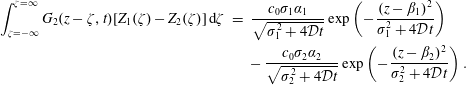 $$\begin{eqnarray}\displaystyle \int _{\unicode[STIX]{x1D701}=-\infty }^{\unicode[STIX]{x1D701}=\infty }G_{2}(z-\unicode[STIX]{x1D701},t)[Z_{1}(\unicode[STIX]{x1D701})-Z_{2}(\unicode[STIX]{x1D701})]\,\text{d}\unicode[STIX]{x1D701} & = & \displaystyle {\displaystyle \frac{c_{0}\unicode[STIX]{x1D70E}_{1}\unicode[STIX]{x1D6FC}_{1}}{\sqrt{\unicode[STIX]{x1D70E}_{1}^{2}+4{\mathcal{D}}t}}}\exp \left(-{\displaystyle \frac{(z-\unicode[STIX]{x1D6FD}_{1})^{2}}{\unicode[STIX]{x1D70E}_{1}^{2}+4{\mathcal{D}}t}}\right)\nonumber\\ \displaystyle & & \displaystyle -\,{\displaystyle \frac{c_{0}\unicode[STIX]{x1D70E}_{2}\unicode[STIX]{x1D6FC}_{2}}{\sqrt{\unicode[STIX]{x1D70E}_{2}^{2}+4{\mathcal{D}}t}}}\exp \left(-{\displaystyle \frac{(z-\unicode[STIX]{x1D6FD}_{2})^{2}}{\unicode[STIX]{x1D70E}_{2}^{2}+4{\mathcal{D}}t}}\right).\qquad\end{eqnarray}$$
 Inserting this result into (B 9), leads to the following expression for  $B_{n}(z,t)$:
 $$\begin{eqnarray}\displaystyle B_{n}(z,t) & = & \displaystyle -{\displaystyle \frac{c_{0}\unicode[STIX]{x03C0}}{\unicode[STIX]{x1D706}_{n}^{2}\text{J}_{0}(\unicode[STIX]{x1D706}_{n})}}\boldsymbol{H}_{1}(\unicode[STIX]{x1D706}_{n})\left[{\displaystyle \frac{\unicode[STIX]{x1D70E}_{1}\unicode[STIX]{x1D6FC}_{1}}{\sqrt{\unicode[STIX]{x1D70E}_{1}^{2}+4{\mathcal{D}}t}}}\exp \left(-{\displaystyle \frac{(z-\unicode[STIX]{x1D6FD}_{1})^{2}}{\unicode[STIX]{x1D70E}_{1}^{2}+4{\mathcal{D}}t}}\right)\right.\nonumber\\ \displaystyle & & \displaystyle -\left.{\displaystyle \frac{\unicode[STIX]{x1D70E}_{2}\unicode[STIX]{x1D6FC}_{2}}{\sqrt{\unicode[STIX]{x1D70E}_{2}^{2}+4{\mathcal{D}}t}}}\exp \left(-{\displaystyle \frac{(z-\unicode[STIX]{x1D6FD}_{2})^{2}}{\unicode[STIX]{x1D70E}_{2}^{2}+4{\mathcal{D}}t}}\right)\right].\end{eqnarray}$$
 Finally, recalling the definition of  $s^{\ast }$ given by (A 30), the final result of this analysis is obtained
 $$\begin{eqnarray}\displaystyle s^{\ast }(z,t) & = & \displaystyle -4\unicode[STIX]{x03C0}c_{0}U\left[{\displaystyle \frac{\unicode[STIX]{x1D70E}_{1}\unicode[STIX]{x1D6FC}_{1}(z-\unicode[STIX]{x1D6FD}_{1})}{(\unicode[STIX]{x1D70E}_{1}^{2}+4{\mathcal{D}}t)^{3/2}}}\exp \left(-{\displaystyle \frac{(z-\unicode[STIX]{x1D6FD}_{1})^{2}}{\unicode[STIX]{x1D70E}_{1}^{2}+4{\mathcal{D}}t}}\right)\right.\nonumber\\ \displaystyle & & \displaystyle -\left.{\displaystyle \frac{\unicode[STIX]{x1D70E}_{2}\unicode[STIX]{x1D6FC}_{2}(z-\unicode[STIX]{x1D6FD}_{2})}{(\unicode[STIX]{x1D70E}_{2}^{2}+4{\mathcal{D}}t)^{3/2}}}\exp \left(-{\displaystyle \frac{(z-\unicode[STIX]{x1D6FD}_{2})^{2}}{\unicode[STIX]{x1D70E}_{2}^{2}+4{\mathcal{D}}t}}\right)\right]\mathop{\sum }_{n=1}^{\infty }{\displaystyle \frac{\boldsymbol{H}_{1}(\unicode[STIX]{x1D706}_{n})}{\unicode[STIX]{x1D706}_{n}^{3}}}{\displaystyle \frac{\text{J}_{3}(\unicode[STIX]{x1D706}_{n})}{\text{J}_{0}(\unicode[STIX]{x1D706}_{n})}}\exp \left(-{\displaystyle \frac{\unicode[STIX]{x1D706}_{n}^{2}{\mathcal{D}}}{a^{2}}}t\right).\nonumber\\ \displaystyle & & \displaystyle\end{eqnarray}$$
B.2 Step function in radial distributions
Consider the situation in which the radial variation in the initial condition happens as a step function so that the functions  $R_{1}$ and $R_{2}$ are defined by
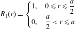 $$\begin{eqnarray}\displaystyle & \displaystyle R_{1}(r)=\left\{\begin{array}{@{}ll@{}}1,\quad & 0\leqslant r\leqslant {\displaystyle \frac{a}{2}}\\ 0,\quad & {\displaystyle \frac{a}{2}}<r\leqslant a\end{array}\right. & \displaystyle\end{eqnarray}$$
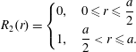 $$\begin{eqnarray}\displaystyle & \displaystyle R_{2}(r)=\left\{\begin{array}{@{}ll@{}}0,\quad & 0\leqslant r\leqslant {\displaystyle \frac{a}{2}}\\ 1,\quad & {\displaystyle \frac{a}{2}}<r\leqslant a.\end{array}\right. & \displaystyle\end{eqnarray}$$
 Applying the spatial averaging operator to (B 15b) leads to  $\langle R_{1}\rangle$ and $\langle R_{2}\rangle$ given by
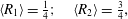 $$\begin{eqnarray}\langle R_{1}\rangle ={\textstyle \frac{1}{4}};\quad \langle R_{2}\rangle ={\textstyle \frac{3}{4}},\end{eqnarray}$$
 which when subtracted from (B 15b) give, for the deviations,  $\tilde{R}_{1}$ and $\tilde{R}_{2}$:
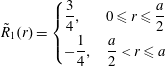 $$\begin{eqnarray}\displaystyle & \displaystyle \tilde{R}_{1}(r)=\left\{\begin{array}{@{}ll@{}}{\displaystyle \frac{3}{4}},\quad & 0\leqslant r\leqslant {\displaystyle \frac{a}{2}}\\ -{\displaystyle \frac{1}{4}},\quad & {\displaystyle \frac{a}{2}}<r\leqslant a\end{array}\right. & \displaystyle\end{eqnarray}$$
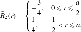 $$\begin{eqnarray}\displaystyle & \displaystyle \tilde{R}_{2}(r)=\left\{\begin{array}{@{}ll@{}}-{\displaystyle \frac{3}{4}},\quad & 0\leqslant r\leqslant {\displaystyle \frac{a}{2}}\\ {\displaystyle \frac{1}{4}},\quad & {\displaystyle \frac{1}{2}}<r\leqslant a.\end{array}\right. & \displaystyle\end{eqnarray}$$ $\tilde{R}_{1}(r)=-\tilde{R}_{2}(r)$, consequently the initial condition for the concentration deviations are now
  $$\begin{eqnarray}\tilde{\unicode[STIX]{x1D711}}(r,z)=[Z_{1}(z)-Z_{2}(z)]\tilde{R}_{1}(r).\end{eqnarray}$$
Recall that we have
 $$\begin{eqnarray}B_{n}(z,t)={\displaystyle \frac{2}{a^{2}\text{J}_{0}^{2}(\unicode[STIX]{x1D706}_{n})}}\int _{\unicode[STIX]{x1D701}=-\infty }^{\unicode[STIX]{x1D701}=\infty }G_{2}(z-\unicode[STIX]{x1D701},t)[Z_{1}(\unicode[STIX]{x1D701})-Z_{2}(\unicode[STIX]{x1D701})]\,\text{d}\unicode[STIX]{x1D701}\int _{r=0}^{r=a}\tilde{R}_{1}(r)\text{J}_{0}\left(\unicode[STIX]{x1D706}_{n}{\displaystyle \frac{r}{a}}\right)r\,\text{d}r.\end{eqnarray}$$
 On the basis of this initial condition,  $B_{n}(z,0)$ can be expressed as
 $$\begin{eqnarray}\displaystyle B_{n}(z,0) & = & \displaystyle {\displaystyle \frac{2}{a^{2}\text{J}_{0}^{2}(\unicode[STIX]{x1D706}_{n})}}\int _{\unicode[STIX]{x1D701}=-\infty }^{\unicode[STIX]{x1D701}=\infty }G_{2}(z-\unicode[STIX]{x1D701},t)[Z_{1}(\unicode[STIX]{x1D701})-Z_{2}(\unicode[STIX]{x1D701})]\,\text{d}\unicode[STIX]{x1D701}\nonumber\\ \displaystyle & & \displaystyle \times \,\left[{\displaystyle \frac{3}{4}}\int _{r=0}^{r=a/2}\text{J}_{0}\left(\unicode[STIX]{x1D706}_{n}{\displaystyle \frac{r}{a}}\right)r\,\text{d}r-{\displaystyle \frac{1}{4}}\int _{r=a/2}^{r=a}\text{J}_{0}\left(\unicode[STIX]{x1D706}_{n}{\displaystyle \frac{r}{a}}\right)r\,\text{d}r\right].\end{eqnarray}$$
Noting that (Olver et al. Reference Olver, Lozier, Boisvert and Clark2010)
 $$\begin{eqnarray}\int \text{J}_{0}\left(\unicode[STIX]{x1D706}_{n}{\displaystyle \frac{r}{a}}\right)r\,\text{d}r={\displaystyle \frac{a}{\unicode[STIX]{x1D706}_{n}}}r\text{J}_{1}\left(\unicode[STIX]{x1D706}_{n}{\displaystyle \frac{r}{a}}\right)+c,\end{eqnarray}$$
then, (B 20) can be simplified to give the following:
 $$\begin{eqnarray}B_{n}(z,0)={\displaystyle \frac{\text{J}_{1}(\unicode[STIX]{x1D706}_{n}/2)}{\unicode[STIX]{x1D706}_{n}\text{J}_{0}^{2}(\unicode[STIX]{x1D706}_{n})}}\int _{\unicode[STIX]{x1D701}=-\infty }^{\unicode[STIX]{x1D701}=\infty }G_{2}(z-\unicode[STIX]{x1D701},t)[Z_{1}(\unicode[STIX]{x1D701})-Z_{2}(\unicode[STIX]{x1D701})]\,\text{d}\unicode[STIX]{x1D701}.\end{eqnarray}$$
 Recalling the previous results for the integrals involving  $Z_{1}$ and $Z_{2}$ given by (B 12), and the definition of $s^{\ast }$ given by (A 30), the following explicit series solution for $s^{\ast }$ is obtained:
 $$\begin{eqnarray}\displaystyle s^{\ast }(z,t) & = & \displaystyle 4c_{0}U\left[{\displaystyle \frac{\unicode[STIX]{x1D70E}_{1}\unicode[STIX]{x1D6FC}_{1}(z-\unicode[STIX]{x1D6FD}_{1})}{(\unicode[STIX]{x1D70E}_{1}^{2}+4{\mathcal{D}}t)^{3/2}}}\exp \left(-{\displaystyle \frac{(z-\unicode[STIX]{x1D6FD}_{1})^{2}}{\unicode[STIX]{x1D70E}_{1}^{2}+4{\mathcal{D}}t}}\right)\right.\nonumber\\ \displaystyle & & \displaystyle -\left.{\displaystyle \frac{\unicode[STIX]{x1D70E}_{2}\unicode[STIX]{x1D6FC}_{2}(z-\unicode[STIX]{x1D6FD}_{2})}{(\unicode[STIX]{x1D70E}_{2}^{2}+4{\mathcal{D}}t)^{3/2}}}\exp \left(-{\displaystyle \frac{(z-\unicode[STIX]{x1D6FD}_{2})^{2}}{\unicode[STIX]{x1D70E}_{2}^{2}+4{\mathcal{D}}t}}\right)\right]\nonumber\\ \displaystyle & & \displaystyle \times \,\mathop{\sum }_{n=1}^{\infty }{\displaystyle \frac{\text{J}_{1}(\unicode[STIX]{x1D706}_{n}/2)\text{J}_{3}(\unicode[STIX]{x1D706}_{n})}{\unicode[STIX]{x1D706}_{n}^{2}J_{0}^{2}(\unicode[STIX]{x1D706}_{n})}}\exp \left(-{\displaystyle \frac{\unicode[STIX]{x1D706}_{n}^{2}{\mathcal{D}}}{a^{2}}}t\right).\end{eqnarray}$$
B.3 Accounting for convection
For  $Pe_{T}\ll 1$, the solutions above should give sufficient estimates for $s^{\ast }$. However, recall that the closure problem was transformed into the coordinate system moving with the velocity of the centre of mass of the system. At asymptotic times, the distribution of solutes is nearly uniform across the radius; thus, the average fluid velocity is identically equal to the mass average velocity. However, in this work we have been investigating the special condition where initially the solute is distributed in two parts, each with different initial mass averaged velocities. This poses some difficulty, because in general the averaged velocity of the centre of mass of the solute is an unknown function of time. This difference between the mass-averaged and average fluid velocities (and the potential problems that it poses) was also identified in the work of Gill & Sankarasubramanian (Reference Gill and Sankarasubramanian1971), Degance & Johns (Reference Degance and Johns1978b), Dentz & Carrera (Reference Dentz and Carrera2007) and Ratnakar & Balakotaiah (Reference Ratnakar and Balakotaiah2011).
For initial-condition-type problems, the mass-averaged velocities can be found from the centre of mass of the moving solute distribution
 $$\begin{eqnarray}\displaystyle & \displaystyle M_{0}=2\unicode[STIX]{x03C0}\int _{r=0}^{r=a}\int _{z=0}^{z=L}\unicode[STIX]{x1D711}(r,z)r\,\text{d}r\,\text{d}z, & \displaystyle\end{eqnarray}$$
 $$\begin{eqnarray}\displaystyle & \displaystyle M_{1,z}(t)={\displaystyle \frac{2\unicode[STIX]{x03C0}}{M_{0}}}\int _{r=0}^{r=a}\int _{z=0}^{z=L}zc(r,z,t)r\,\text{d}r\,\text{d}z. & \displaystyle\end{eqnarray}$$
 $$\begin{eqnarray}\langle v_{z,M}\rangle ={\displaystyle \frac{\unicode[STIX]{x2202}M_{1}(t)}{\unicode[STIX]{x2202}t}}.\end{eqnarray}$$
 Before moving on, it is worth recalling that, among the simplifications adopted in this work, it was assumed that the term  $\tilde{v}_{z}\unicode[STIX]{x2202}\tilde{c}/\unicode[STIX]{x2202}z$ and its spatial average are negligible in comparison to the radial diffusive term (valid for $Pe(a/L_{0})=\boldsymbol{O}(1)$). In the material that follows, we make corrections to the coordinate used to displace the solutions, but we do not alter the value $U$ that appears in these solutions. The following constraint is adopted to indicate under what conditions this assumption is valid:
 $$\begin{eqnarray}(\langle v_{z,M}\rangle |_{t}-U){\displaystyle \frac{\unicode[STIX]{x2202}\langle c\rangle }{\unicode[STIX]{x2202}z}}\ll \tilde{v}_{z}{\displaystyle \frac{\unicode[STIX]{x2202}\tilde{c}}{\unicode[STIX]{x2202}z}}\end{eqnarray}$$
or, making conventional order-of-magnitude estimates, a reasonable constraint is
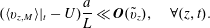 $$\begin{eqnarray}(\langle v_{z,M}\rangle |_{t}-U){\displaystyle \frac{a}{L}}\ll \boldsymbol{O}(\tilde{v}_{z}),\quad \forall (z,t).\end{eqnarray}$$
 Here, it has been assumed that reasonable estimates of the characteristic lengths of variations for  $\tilde{c}$ and $\langle c\rangle$ are $a$ and $L$, respectively. In the solutions below, it will be apparent that this constraint is easily met for the particular initial conditions studied.
It is convenient to denote the portion of the total initial mass per unit length of the tube given by each of the two parts of the initial condition be specified by
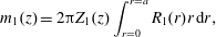 $$\begin{eqnarray}\displaystyle & \displaystyle m_{1}(z)=2\unicode[STIX]{x03C0}Z_{1}(z)\int _{r=0}^{r=a}R_{1}(r)r\,\text{d}r, & \displaystyle\end{eqnarray}$$
 $$\begin{eqnarray}\displaystyle & \displaystyle m_{2}(z)=2\unicode[STIX]{x03C0}Z_{2}(z)\int _{r=0}^{r=a}R_{2}(r)r\,\text{d}r. & \displaystyle\end{eqnarray}$$
From the above definitions, the mass weightings for the two portions of the initial condition are defined as
 $$\begin{eqnarray}\displaystyle & \displaystyle \unicode[STIX]{x1D714}_{1}(r)={\displaystyle \frac{Z_{1}(z)}{m_{1}(z)}}R_{1}(r)=R_{1}(r)\left(2\unicode[STIX]{x03C0}\int _{r=0}^{r=a}R_{1}(r)r\,\text{d}r\right)^{-1}, & \displaystyle\end{eqnarray}$$
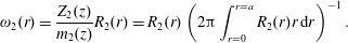 $$\begin{eqnarray}\displaystyle & \displaystyle \unicode[STIX]{x1D714}_{2}(r)={\displaystyle \frac{Z_{2}(z)}{m_{2}(z)}}R_{2}(r)=R_{2}(r)\left(2\unicode[STIX]{x03C0}\int _{r=0}^{r=a}R_{2}(r)r\,\text{d}r\right)^{-1}. & \displaystyle\end{eqnarray}$$
 $$\begin{eqnarray}\displaystyle & \displaystyle \langle v_{z,M}\rangle _{1}(t=0)=2\unicode[STIX]{x03C0}\int _{r=0}^{r=a}\unicode[STIX]{x1D714}(w)_{1}(r)v_{z}(r)r\,\text{d}r, & \displaystyle\end{eqnarray}$$
 $$\begin{eqnarray}\displaystyle & \displaystyle \langle v_{z,M}\rangle _{2}(t=0)=2\unicode[STIX]{x03C0}\int _{r=0}^{r=a}\unicode[STIX]{x1D714}_{2}(r)v_{z}(r)r\,\text{d}r. & \displaystyle\end{eqnarray}$$
The difficulty now is to determine a time scale for which the initial condition spreads sufficiently to sample the entire velocity distribution. To this end, consider the following rough estimate for the variance of the initial condition corresponding to an unbounded two-dimensional field:
 $$\begin{eqnarray}\unicode[STIX]{x1D70E}(t)=\sqrt{4{\mathcal{D}}t}.\end{eqnarray}$$
 Hence, the interest is to find a time,  $t_{d}^{\ast }$, for which $\unicode[STIX]{x1D70E}=a$, i.e.
 $$\begin{eqnarray}t_{d}^{\ast }={\displaystyle \frac{a^{2}}{4{\mathcal{D}}}},\end{eqnarray}$$
 which is referred to as the diffusive time scale. With this time scale established, it is now necessary to develop a model that describes how the average velocity of each of the two non-uniform initial condition contributions ( $R_{1}$ and $R_{2}$) relaxes from its initial average to the average fluid velocity over the time $t_{d}^{\ast }$. Since the process is diffusion driven, a simple square-root-of-time behaviour seems reasonable. Our proposed model is approximate, but is correct at the initial and asymptotic times. Essentially, we assume that the average solute velocity transitions from its value at $t=0$ to the average fluid velocity, $U$, over the time scale $t_{d}^{\ast }$ following a $t^{1/2}$ law.
B.3.1 Linear distribution
For the linear radial distribution in the initial condition, the corresponding weighting functions are
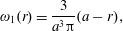 $$\begin{eqnarray}\displaystyle & \displaystyle \unicode[STIX]{x1D714}_{1}(r)={\displaystyle \frac{3}{a^{3}\unicode[STIX]{x03C0}}}(a-r), & \displaystyle\end{eqnarray}$$
 $$\begin{eqnarray}\displaystyle & \displaystyle \unicode[STIX]{x1D714}_{2}(r)={\displaystyle \frac{3}{2a^{3}\unicode[STIX]{x03C0}}}r. & \displaystyle\end{eqnarray}$$
 $$\begin{eqnarray}\displaystyle & \displaystyle \langle v_{z,M}\rangle _{1}(t=0)={\textstyle \frac{7}{5}}U, & \displaystyle\end{eqnarray}$$
 $$\begin{eqnarray}\displaystyle & \displaystyle \langle v_{z,M}\rangle _{2}(t=0)={\textstyle \frac{4}{5}}U. & \displaystyle\end{eqnarray}$$ $t_{d}^{\ast }$, the transient velocities associated with the linear initial distributions $R_{1}$ and $R_{2}$ are
  $$\begin{eqnarray}\displaystyle & \displaystyle \langle v_{z,M}\rangle _{1}(t)=\left\{\begin{array}{@{}ll@{}}{\displaystyle \frac{7}{5}}U-{\displaystyle \frac{2}{5}}U\left({\displaystyle \frac{t}{t_{d}^{\ast }}}\right)^{1/2},\quad & \text{for }t<t_{d}^{\ast },\\ U,\quad & \text{for }t\geqslant t_{d}^{\ast },\end{array}\right. & \displaystyle\end{eqnarray}$$
 $$\begin{eqnarray}\displaystyle & \displaystyle \langle v_{z,M}\rangle _{2}(t)=\left\{\begin{array}{@{}ll@{}}{\displaystyle \frac{4}{5}}U+{\displaystyle \frac{1}{5}}U\left({\displaystyle \frac{t}{t_{d}^{\ast }}}\right)^{1/2},\quad & \text{for }t<t_{d}^{\ast },\\ U,\quad & \text{for }t\geqslant t_{d}^{\ast }.\end{array}\right. & \displaystyle\end{eqnarray}$$

The corresponding expressions for the translations created by these time-varying velocity fields are now given by
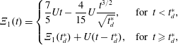 $$\begin{eqnarray}\displaystyle & \displaystyle \unicode[STIX]{x1D6EF}_{1}(t)=\left\{\begin{array}{@{}ll@{}}{\displaystyle \frac{7}{5}}Ut-{\displaystyle \frac{4}{15}}U{\displaystyle \frac{t^{3/2}}{\sqrt{t_{d}^{\ast }}}},\quad & \text{for }t<t_{d}^{\ast },\\ \unicode[STIX]{x1D6EF}_{1}(t_{d}^{\ast })+U(t-t_{d}^{\ast }),\quad & \text{for }t\geqslant t_{d}^{\ast },\end{array}\right. & \displaystyle\end{eqnarray}$$
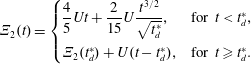 $$\begin{eqnarray}\displaystyle & \displaystyle \unicode[STIX]{x1D6EF}_{2}(t)=\left\{\begin{array}{@{}ll@{}}{\displaystyle \frac{4}{5}}Ut+{\displaystyle \frac{2}{15}}U{\displaystyle \frac{t^{3/2}}{\sqrt{t_{d}^{\ast }}}},\quad & \text{for }t<t_{d}^{\ast },\\ \unicode[STIX]{x1D6EF}_{2}(t_{d}^{\ast })+U(t-t_{d}^{\ast }),\quad & \text{for }t\geqslant t_{d}^{\ast }.\end{array}\right. & \displaystyle\end{eqnarray}$$
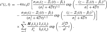 $$\begin{eqnarray}\displaystyle s^{\ast }(z,t) & = & \displaystyle -4\unicode[STIX]{x03C0}c_{0}U\left[{\displaystyle \frac{\unicode[STIX]{x1D70E}_{1}\unicode[STIX]{x1D6FC}_{1}(z-\unicode[STIX]{x1D6EF}_{1}(t)-\unicode[STIX]{x1D6FD}_{1})}{(\unicode[STIX]{x1D70E}_{1}^{2}+4{\mathcal{D}}t)^{3/2}}}\exp \left(-{\displaystyle \frac{(z-\unicode[STIX]{x1D6EF}_{1}(t)-\unicode[STIX]{x1D6FD}_{1})^{2}}{\unicode[STIX]{x1D70E}_{1}^{2}+4{\mathcal{D}}t}}\right)\right.\nonumber\\ \displaystyle & & \displaystyle -\left.{\displaystyle \frac{\unicode[STIX]{x1D70E}_{2}\unicode[STIX]{x1D6FC}_{2}(z-\unicode[STIX]{x1D6EF}_{2}(t)-\unicode[STIX]{x1D6FD}_{2})}{(\unicode[STIX]{x1D70E}_{2}^{2}+4{\mathcal{D}}t)^{3/2}}}\exp \left(-{\displaystyle \frac{(z-\unicode[STIX]{x1D6EF}_{2}(t)-\unicode[STIX]{x1D6FD}_{2})^{2}}{\unicode[STIX]{x1D70E}_{2}^{2}+4{\mathcal{D}}t}}\right)\right]\nonumber\\ \displaystyle & & \displaystyle \times \,\mathop{\sum }_{n=1}^{\infty }{\displaystyle \frac{\boldsymbol{H}_{1}(\unicode[STIX]{x1D706}_{n})}{\unicode[STIX]{x1D706}_{n}^{3}}}{\displaystyle \frac{\text{J}_{3}(\unicode[STIX]{x1D706}_{n})}{\text{J}_{0}(\unicode[STIX]{x1D706}_{n})}}\exp \left(-{\displaystyle \frac{\unicode[STIX]{x1D706}_{n}^{2}{\mathcal{D}}}{a^{2}}}t\right).\end{eqnarray}$$
B.3.2 Step distribution
For the step radial distribution, the weighting functions are  $\unicode[STIX]{x1D714}_{1}=4F_{1}/(\unicode[STIX]{x03C0}a^{2})$ and $\unicode[STIX]{x1D714}_{2}=4F_{2}/(3\unicode[STIX]{x03C0}a^{2})$. The associated velocities are given by
 $$\begin{eqnarray}\displaystyle & \displaystyle \langle v_{z,M}\rangle _{1}(t=0)={\textstyle \frac{7}{4}}U, & \displaystyle\end{eqnarray}$$
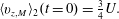 $$\begin{eqnarray}\displaystyle & \displaystyle \langle v_{z,M}\rangle _{2}(t=0)={\textstyle \frac{3}{4}}U. & \displaystyle\end{eqnarray}$$ $t_{d}^{\ast }$, the transient velocities associated with the initial distributions $R_{1}$ and $R_{2}$ are found to be
 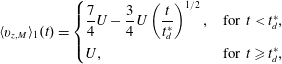 $$\begin{eqnarray}\displaystyle & \displaystyle \langle v_{z,M}\rangle _{1}(t)=\left\{\begin{array}{@{}ll@{}}{\displaystyle \frac{7}{4}}U-{\displaystyle \frac{3}{4}}U\left({\displaystyle \frac{t}{t_{d}^{\ast }}}\right)^{1/2},\quad & \text{for }t<t_{d}^{\ast },\\ U,\quad & \text{for }t\geqslant t_{d}^{\ast },\end{array}\right. & \displaystyle\end{eqnarray}$$
 $$\begin{eqnarray}\displaystyle & \displaystyle \langle v_{z,M}\rangle _{2}(t)=\left\{\begin{array}{@{}ll@{}}{\displaystyle \frac{3}{4}}U+{\displaystyle \frac{1}{4}}U\left({\displaystyle \frac{t}{t_{d}^{\ast }}}\right)^{1/2},\quad & \text{for }t<t_{d}^{\ast },\\ U,\quad & \text{for }t\geqslant t_{d}^{\ast }.\end{array}\right. & \displaystyle\end{eqnarray}$$ $Z(t)$, it follows that
 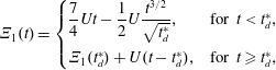 $$\begin{eqnarray}\displaystyle & \displaystyle \unicode[STIX]{x1D6EF}_{1}(t)=\left\{\begin{array}{@{}ll@{}}{\displaystyle \frac{7}{4}}Ut-{\displaystyle \frac{1}{2}}U{\displaystyle \frac{t^{3/2}}{\sqrt{t_{d}^{\ast }}}},\quad & \text{for }t<t_{d}^{\ast },\\ \unicode[STIX]{x1D6EF}_{1}(t_{d}^{\ast })+U(t-t_{d}^{\ast }),\quad & \text{for }t\geqslant t_{d}^{\ast },\end{array}\right. & \displaystyle\end{eqnarray}$$
 $$\begin{eqnarray}\displaystyle & \displaystyle \unicode[STIX]{x1D6EF}_{2}(t)=\left\{\begin{array}{@{}ll@{}}{\displaystyle \frac{3}{4}}Ut+{\displaystyle \frac{1}{6}}U{\displaystyle \frac{t^{3/2}}{\sqrt{t_{d}^{\ast }}}},\quad & \text{for }t<t_{d}^{\ast },\\ \unicode[STIX]{x1D6EF}_{2}(t_{d}^{\ast })+U(t-t_{d}^{\ast }),\quad & \text{for }t\geqslant t_{d}^{\ast }.\end{array}\right. & \displaystyle\end{eqnarray}$$
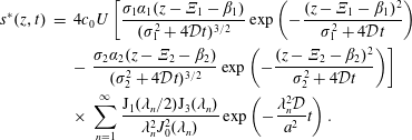 $$\begin{eqnarray}\displaystyle s^{\ast }(z,t) & = & \displaystyle 4c_{0}U\left[{\displaystyle \frac{\unicode[STIX]{x1D70E}_{1}\unicode[STIX]{x1D6FC}_{1}(z-\unicode[STIX]{x1D6EF}_{1}-\unicode[STIX]{x1D6FD}_{1})}{(\unicode[STIX]{x1D70E}_{1}^{2}+4{\mathcal{D}}t)^{3/2}}}\exp \left(-{\displaystyle \frac{(z-\unicode[STIX]{x1D6EF}_{1}-\unicode[STIX]{x1D6FD}_{1})^{2}}{\unicode[STIX]{x1D70E}_{1}^{2}+4{\mathcal{D}}t}}\right)\right.\nonumber\\ \displaystyle & & \displaystyle -\left.{\displaystyle \frac{\unicode[STIX]{x1D70E}_{2}\unicode[STIX]{x1D6FC}_{2}(z-\unicode[STIX]{x1D6EF}_{2}-\unicode[STIX]{x1D6FD}_{2})}{(\unicode[STIX]{x1D70E}_{2}^{2}+4{\mathcal{D}}t)^{3/2}}}\exp \left(-{\displaystyle \frac{(z-\unicode[STIX]{x1D6EF}_{2}-\unicode[STIX]{x1D6FD}_{2})^{2}}{\unicode[STIX]{x1D70E}_{2}^{2}+4{\mathcal{D}}t}}\right)\right]\nonumber\\ \displaystyle & & \displaystyle \times \,\mathop{\sum }_{n=1}^{\infty }{\displaystyle \frac{\text{J}_{1}(\unicode[STIX]{x1D706}_{n}/2)\text{J}_{3}(\unicode[STIX]{x1D706}_{n})}{\unicode[STIX]{x1D706}_{n}^{2}J_{0}^{2}(\unicode[STIX]{x1D706}_{n})}}\exp \left(-{\displaystyle \frac{\unicode[STIX]{x1D706}_{n}^{2}{\mathcal{D}}}{a^{2}}}t\right).\end{eqnarray}$$


 Open access