


1. Introduction
Linguistic complexity is a meta-property of language that is important to our conception of how linguistic features interact and evolve with regard to forming structurally more or less complex patterns. However, the very nature of this complexity meta-property is still debated, specifically how it is constituted, how it behaves and how different complexity levels determine certain structures in languages. A major question in studies of linguistic complexity is whether the complexity of certain linguistic features correlates with the complexity of other features (sometimes called ‘cumulative’ complexity), or if it instead exhibits a trade-off behaviour. The present study aims to use artificial neural networksFootnote 1 and Bayesian structural equation models to derive a latentFootnote 2 complexity measure for each language in cross-linguistic data, which can in turn be used to analyse the interactions between different features of phonological complexity alongside common dimensionality-reduction methods such as principal component analysis (PCA). Dimensionality reduction is the process of projecting a higher-dimensional space onto a lower-dimensional one.
Complexity does not have a single agreed-upon definition, but rather is seen as a complex and multifaceted property (for a comprehensive overview, see Nichols Reference Nichols, Sampson, Gil and Trudgill2009; Arkadiev & Gardani Reference Arkadiev, Gardani, Arkadiev and Gardani2020). Phonological complexity can be described as representing the number and types of discriminative (or contrastive) phonological properties or units (e.g., distinctive features, phonemes, syllable types) in a given language. In this study, phonological complexity is viewed as a type of enumerative complexity or, more specifically, the distribution of sound segments per language across the available phonological features. This investigation draws on enumerative complexity (cf. Anderson Reference Anderson, Baerman, Brown and Corbett2015; Baerman et al. Reference Baerman, Brown, Corbett, Baerman, Brown and Corbett2015; Cotterell et al. Reference Cotterell, Kirov, Hulden and Eisner2019), and on inventory complexity (a specific case of enumerative complexity) in particular. This computational definition of complexity, as proposed here, is set apart from other definitions of linguistic complexity that instead focus on sociolinguistic criteria and considerations of learnability (e.g., computational approaches such as Chen & Meurers Reference Chen, Meurers, Brunato, Dell’Orletta, Venturi, François and Blache2016). The latter is often called ‘relative complexity’ and is defined as a language’s complexity (e.g., in learnability) from the viewpoint of a user of a different language (Becerra-Bonache et al. Reference Becerra-Bonache, Christiansen, Jiménez-López, Becerra-Bonache, Jiménez-López, Martín-Vide and Torrens-Urrutia2018). According to this working definition, a maximally complex language has the maximum number of phonemes equally distributed across all phonologically producible features.Footnote 3 A minimally complex language would have very few phonological segments distributed across very few phonological features.Footnote 4
The cumulative complexity hypothesis is the notion that phonological complexity is positively autocorrelated (i.e., complexity in one aspect positively correlates with complexity in another). Studies that involve featural or inventory complexity often find a cumulative behaviour between segments, for example, Maddieson (Reference Maddieson2005b, Reference Maddieson2009, Reference Maddieson2011; see discussion below). A good breakdown of the debate can be found in, for example, Oh (Reference Oh2015) and Kusters (Reference Kusters2003). Further, Joseph (Reference Joseph2021) discusses general issues related to methods and approaches to measure linguistic complexity.
Conversely, it has been stated in the past that all languages are equally complex (the equi-complexity hypothesis, on which see Hockett Reference Hockett1958) which would entail diachronic trade-off behaviour between complexity features, a proposition which has been challenged by some. For example, Kusters (Reference Kusters2003: 11–12) rejects the notion that all languages have the same level of complexity. Trudgill (Reference Trudgill2011), recently re-examined by Walkden & Breitbarth (Reference Walkden and Breitbarth2019), investigates sociolinguistic factors in complexity, challenging equi-complexity assumptions. Investigations into equi-complexity often seek to find complexity trade-offs between different domains of linguistics, since these would be evidence in support of equi-complexity.Footnote 5
Most studies that find a trade-off behaviour in phonological contexts focus on phonological complexity outside of inventory or feature complexity. For example, Pellegrino et al. (Reference Pellegrino, Coupé and Marsico2011) investigate the implications of a trade-off between speech rate and information density arising from syllable complexity. They find that the syllable complexity of a language can be measured using an inventory of syllables and their frequency of use (obtained from a speech or text corpus). The importance of considering frequencies has been discussed and analysed by Macklin-Cordes & Round (Reference Macklin-Cordes and Round2020; here phoneme frequencies). Starting from the findings in Pellegrino et al. (Reference Pellegrino, Coupé and Marsico2011), Pimentel et al. (Reference Pimentel, Roark and Cotterell2020) find a trade-off between phonological complexity (measured in this case in bits per phoneme) and word length. Further, Fenk-Oczlon & Fenk (Reference Fenk-Oczlon and Fenk2014) show phonotactic trade-offs between syllable complexity and the number of syllables per word and per clause.
While much of the debate mainly centres on inter-domain cumulativity or equi-complexity, this analysis focusses on investigating within-domain phonological complexity with computational means. In this article, I propose a computational definition of complexity by deriving phonological complexity as a latent factor from the data to investigate its shape and behaviour. Beyond providing a computational measure of complexity for each language based on the present phonological features, the approach allows for an investigation into what features are positively or negatively associated with increased or decreased complexity. To compare this to other methods with similar aims, I further use PCA, a commonly used dimensionality reduction algorithm. If phonological complexity is cumulative within its domain, we would expect to see all phonological features positively associated with overall phonological complexity.
Phonological complexity has been investigated in a variety of studies; the following discussion therefore focusses on enumerative/quantitative approaches to measuring phonological complexity. Maddieson (Reference Maddieson2011), for example, cross-linguistically analyses enumerative complexity (such as inventory size, number of vowels, consonants) in the context of occurrence frequency, co-occurrence and geographical variables such as best-origin distance (cf. Atkinson Reference Atkinson2011). Maddieson (Reference Maddieson2005b), on the other hand, compares enumerative measures like inventory size with an ordered categorical measure of syllable complexity, while Maddieson (Reference Maddieson2009) compares languages as to the complexity of individual phonemes and syllable types. Rice & Avery (Reference Rice and Avery1993) provide discussion and analysis of the relation between inventory size and segment complexity, investigating the factors involved in the complexification of larger systems. Previous studies have further introduced several ways to analyse complexity by quantitative means (Oh et al. Reference Oh, Pellegrino, Marsico, Coupé, Wielfaert, Heylen and Speelman2013; Oh Reference Oh2015) using computational (e.g., Blache Reference Blache, Bel-Enguix, Dahl and Dolores Jiménez-López2011) and correlational methods (e.g., Maddieson Reference Maddieson2005a; Shosted Reference Shosted2006). Some take an information-theoretic approach (e.g., Pellegrino et al. Reference Pellegrino, Coupé and Marsico2007; Juola Reference Juola, Miestamo, Sinnemäki and Karlsson2008; Ehret & Szmrecsanyi Reference Ehret, Szmrecsanyi, Baechler and Seiler2016), focus on phonotactics (e.g., Pimentel et al. Reference Pimentel, Roark and Cotterell2020), or analyse linguistic inventories directly (e.g., Bane Reference Bane2008). However, analysing complexity quantitatively is intricate, as several studies find. Chitoran & Cohn (Reference Chitoran and Cohn2009), for example, highlight the importance of the distinction between phonetic and phonological complexity, while others such as Sinnemäki (Reference Sinnemäki2011) raise questions about the comparability of different complexity measures. Similar patterns have also been analysed by, for example, Maddieson (Reference Maddieson2011).
Notably, linguistic complexity (and phonological complexity more specifically) has also been approached directly from the angle of the distribution of linguistic elements (e.g., phonemes, morphemes, lexemes), rather than by measuring complexity as the general occurrence frequency and distribution of individual linguistic properties. Entropy-based conceptualisations, for example, focus on how much entropy is contained in a language. Since entropy itself is a measure of predictability, high-entropy systems are less predictably structured (e.g., they have fewer structured patterns in general) and low-entropy systems contain more predictable patterns. Applied to natural language, low-entropy languages are languages that have fewer and more repeating overall patterns (e.g., allowing only CV syllables, or having few phonemes and many restrictions on their distribution), whereas high-entropy languages are those with many different patterns (e.g., freer word order, or many phonemes that are less predictably distributed across the lexicon). Febres et al. (Reference Febres, Jaffé and Gershenson2015), for example, investigate textual entropy for different natural and artificial languages, finding that entropy is a useful discriminator between the languages English and Spanish. Similarly, Baumann et al. (Reference Baumann, Kaźmierski and Matzinger2021: 700) demonstrate that phonotactic structures can be analysed in terms of their behaviour regarding Zipf’s and Heaps’ scaling laws, concluding, among other things, that taking token frequency into account aids in making complexity measures more robust. Other approaches focus on concepts of reducibility – that is, complexity defined by the information content in an object (such as a language or a text). For example, Bane (Reference Bane2008) reviews and discusses the use of Kolmogorov complexity, which, at its core, conceptualises complexity as the minimal length of description necessary to fully describe an entity. This is more commonly applied in computer science, where Kolmogorov complexity describes the minimal size of computer code needed to produce an output. The code needed to describe a simply structured sequence of low entropy is shorter than the code needed to describe a random sequence without structure. Here, compression algorithms (such as are used for reducing the storage size of images or other files) are a related concept, as a maximally efficient compression algorithm condenses information into the minimal description needed to reconstruct the original object.
The computational models used in this article derive the latent complexity value for each language from enumerations of phonemes and features, and so the form of complexity they measure is based solely on these inputs. It thus captures only the aspect of phonological complexity which consists of the features and their interactions in the phonemic inventory; it does not encompass other aspects of phonological complexity, such as learnability or the relative ease of perception and production of different phonemes. §§3.2 and 5.1 provide a more in-depth definition and discussion of what the latent phonological complexity measure captures.
As mentioned above, this is an exclusively within-domain complexity study. Cross-domain trade-offs are not investigated directly, yet the proposals made here may be used for further inquiry into potentially similar effects in other domains. This computational approach presented here is not intended to supersede or replace the other definitions, since it focusses on a specific aspect of complexity concerning the interactions between phonological features. Those interactions can not only yield important insights into cumulativity or trade-off relationships between individual features, but can also shed light on which phonological features are most associated with higher or lower complexity, and which features are correlated with this effect. For example, there are previous findings linking the cross-linguistic rarity of phonological features and the size of phonemic inventories (e.g., Clements Reference Clements, Raimy and Cairns2009: 42), itself an indicator of higher complexity. Moreover, there seems to be a link between the occurrence of more general features and more specialized ones (see Lindblom & Maddieson Reference Lindblom and Maddieson1988; Bybee & Easterday Reference Bybee and Easterday2022). In other studies, we find more specific proposals about the relation between specific features and broader complexity measures (e.g., Maddieson Reference Maddieson2005b). In §4.1, the model results are discussed specifically in connection with these findings.
Further, the goals of this investigation are: (a) to outline the latent variable/PCA approach, demonstrate how it can be implemented and present what results it can produce; and (b) to analyse an enumerative phonological data set using this method so as to explore the implications for phonological complexity research.
2. Data
The data for this study were drawn from the phonological database PHOIBLE (Moran & McCloy Reference Moran and McCloy2019). This database records phonological segments and their features for each of 2,886 doculects representing 2,059 languages. Each doculect is one description of a language; 827 of the languages in the database are represented in multiple descriptions. For each doculect, the features were aggregated by summing the number of phonemes that exhibit a certain feature, yielding counts for each feature in each language which indicate how many phonemes have that feature. If, for example, a language has 11 phonemes that exhibit the feature [dorsal], the segment count for [dorsal] for this language would be 11.
The data set uses 36 features, as illustrated in (1). (1) shows the counts for Rotokas, which has the phoneme inventory in Table 1. For example, Rotokas has six segments for which the feature [sonorant] is indicated in PHOIBLE, but no segments for which [tone] is recorded. The final data set comprises 2,886 surveys, each of which has segment counts for each of the 36 features in (1).
Phonological inventory of Rotokas following Firchow & Firchow (Reference Firchow and Firchow1969), the source used in PHOIBLE.


As mentioned above, PHOIBLE contains different surveys from different contributors for each language, sometimes with large discrepancies between them. Each survey constitutes a doculect which describes a language that might be covered by other surveys. This is, first of all, an advantage since it increases the number of available inventories and, even more importantly, fewer languages in the database are thus represented solely by one surveyor’s decisions, which diversifies the material. Because of the sometimes large discrepancies in per-feature segment counts between different doculects of the same language, it is important to highlight how different doculects were treated in the study. There were no missing values in the data: PHOIBLE provides a list of phonemes in every language’s inventory as determined by the individual surveyors. It further provides a list containing every phoneme reported in any survey, along with its distinctive features. Missing values can therefore only occur if a surveyor fails to record one or more phonemes in a particular language. This, however, would need to be determined on a per-language basis and falls broadly under differences between doculects (discussed above).
For the computational analysis, the doculects were left in their raw form; the computational model thus treats every doculect as its own data point. The reason for this is that the computational approaches are not affected by discrepancies between doculects describing the same language as long as each doculect’s inventory is internally coherent. This is because the models operate on the inventory-internal relationships between per-feature segment counts (see §3.2). In other words, since the latent variable is established from the interrelationships of segment counts within a doculect, different surveys that count phonemes differently but are internally coherent do not affect the model or the overall results concerning, for example, the relative importance of various features. For this reason, the different doculects were not averaged or excluded for every language in the analysis.
Where the doculect discrepancies can cause problems is when model results from different doculects describing the same language are compared. The model may thus show different latent complexity values for this language based on the different doculects. To compare complexities between languages, we can therefore compare doculects from the same source. Moreover, the imbalance between languages that occur once in the data set and the languages that occur multiple times as doculects is rather small, with the maximum number of doculects per language being 11 (Ossetian) and the total count of languages represented by five or more doculects being 29 (1.4% of all languages in the data set). Hence, it is unlikely that those languages impact the final results to a meaningful degree.
It is important to note at this point that the choice to keep different doculects of the same language in the data set is made to mitigate the issues that stem from the multi-surveyor data set. However, for the computational method specifically, the main requirement for the models to work is that the surveys are internally consistent within each language. This means that from the computational perspective, this is the best choice, since the alternative would be to eliminate individual duplicate languages from the data set. In that case, the problem would be to decide which doculects to keep and which to discard. This would then be followed by the question of how to handle the resulting imbalance and pose the question of whether some contributors would need to be removed entirely, thus limiting the size of the data set and the breadth of its applicability.
3. Model setups
To investigate how phonological features behave vis-à-vis complexity, we can analyse phonological complexity as a latent variable and as a dimensionality reduction problem. Recall that a latent variable can be constructed from feature count data as a ‘hidden’ property affecting all phonological feature counts (see §3.2), while dimensionality reduction (here done using PCA) collapses dimensions and can measure the linear relationships between the variables (see §3.1). To get the full picture, we can apply and compare the neural network, Bayesian and PCA models to see which results are different or common between them.
3.1. Principal component analysis
PCA is a widely used method for dimensionality reduction, in which a higher-dimensional data set is transformed to have lower dimensions. Concretely, a data set with any number of variables n can be transformed into a data set with any number of dimensions m, where $m < n$
. This is done by projecting the existing dimensions onto principal components, the set of chosen dimensions of size m. The goal is to preserve the variance between the original variables as well as possible. In other words, it seeks to reduce the number of dimensions such that the least information about the relative position of the data points is lost in the process. This would, for example, chiefly reduce dimensions that account for the least variance in the data set, which can occur when two dimensions are highly correlated.
$m < n$
. This is done by projecting the existing dimensions onto principal components, the set of chosen dimensions of size m. The goal is to preserve the variance between the original variables as well as possible. In other words, it seeks to reduce the number of dimensions such that the least information about the relative position of the data points is lost in the process. This would, for example, chiefly reduce dimensions that account for the least variance in the data set, which can occur when two dimensions are highly correlated.
PCA is in practice an iterative process in which the one vector in the high-dimensional space is identified that maximizes the variance in the data set. This initial vector is then the first principal component (PC1). For further principal components, this process is repeated with the remaining variance once PC1 is accounted for. Figure 1 illustrates this process with a two-dimensional toy data set.
Left: two possible vectors constructed for a two-dimensional toy data set and the distance of each data point to its projection on the respective vector (dashed lines). Right: distribution of the point projections on the two vectors.

Here, we can see two different hypothetical vectors constructed for a two-dimensional toy data set. The bottom vector shows higher overall distances of the data points to the line, which means that less variance can be accounted for. We can see in the right column that when we project the data points onto the chosen vectors, there is greater residual variance in the top projection than in the bottom. Hence, we can say that the top vector preserves more information about the relative positions of the data points. In addition, the original data set shows two clusters of 10 data points each, which are preserved as clusters in the top vector, while in the bottom projection, the distinction between the clusters is not preserved.
Each principal component can be represented as a linear combination of contributing variables, allowing us to quantify the contribution of each input dimension by determining its slope in the corresponding component. Figure 2 shows a sketch of the underlying principle behind this linear combination of dimensions.
Sketch of a single principal component $PC$
, which is a linear combination of dimensions
$PC$
, which is a linear combination of dimensions $D_1$
,
$D_1$
, $D_2$
and
$D_2$
and $D_3$
.
$D_3$
.

When constructing a vector for a given principal component $PC$
, we can measure the linear relationship of each dimension
$PC$
, we can measure the linear relationship of each dimension $D_1$
,
$D_1$
, $D_2$
and
$D_2$
and $D_3$
with this vector. If, for example,
$D_3$
with this vector. If, for example, $D_1$
is associated with the vector through a positive factor, we can say
$D_1$
is associated with the vector through a positive factor, we can say $PC$
and
$PC$
and $D_1$
mutually increase or decrease. This means that we can directly compare the dimensions vis-à-vis their influence on the principal component. For the analysis at hand, there is only one principal component (PC1), to make the results comparable to the other two model types.
$D_1$
mutually increase or decrease. This means that we can directly compare the dimensions vis-à-vis their influence on the principal component. For the analysis at hand, there is only one principal component (PC1), to make the results comparable to the other two model types.
3.2. Deriving a latent complexity variable
The latent variable approach, despite yielding similar insights to those of PCA into associations between variables, is different in many regards. In a hypothetical data set containing languages with numerical properties A, B and C, we assume a latent variable L influences each language’s value of each of these properties (as schematised in Figure 3). A deep neural network or a Bayesian model can infer the individual effects of L on A, B and C relative to the other effects, and the estimate of L that the network calculates is to be understood as the effect of L on the outcome relative to all other effects.
Sketch of a latent variable L and its effects on a set of three variables $\{A, B, C\}$
.
$\{A, B, C\}$
.

For example, let the values of the observed variables be $A = 1$
,
$A = 1$
, $B = -1$
,
$B = -1$
, $C = 0$
, and let the effects be
$C = 0$
, and let the effects be $L \rightarrow A = 0.5$
,
$L \rightarrow A = 0.5$
, $L \rightarrow B = -0.5$
,
$L \rightarrow B = -0.5$
, $L \rightarrow C = 0$
. If we assume a linear relationship, the latent variable can be constructed to be
$L \rightarrow C = 0$
. If we assume a linear relationship, the latent variable can be constructed to be $2$
.Footnote
6
If this is applied to multiple data points of all segment counts A, B and C, the latent variable can be calculated to be an abstract representation of all input feature counts.
$2$
.Footnote
6
If this is applied to multiple data points of all segment counts A, B and C, the latent variable can be calculated to be an abstract representation of all input feature counts.
Following this principle, a latent variable is the ‘common cause’ of all descendant variables and thus a single-variable representation of the system. Structurally, it is the reverse process of PCA. While PCA builds up a linear combination of the input variables and maps it onto a lower-dimensional space (a single dimension in this case), latent variable approaches construct a maximally informative latent variable of which the higher-dimensional variables are linear or nonlinear functions. Crucially, latent variable approaches can both analyse the relations between the per-feature segment counts and derive a latent variable.
This latent representation is different from, but related to, the sum of all phonological features in a language, since it considers the individual input feature counts to be linear or nonlinear functions of the latent values instead of raw aggregates. This does not mean, however, that the overall number of features is entirely ignored, since the encoding does capture the fact that having more different features and more segments increases complexity.Footnote 7 In this vein, the nature of the approach (phonological vs. phonetic) is thus determined by the nature of the input data. PHOIBLE’s feature set is phonological, using a mapping from IPA to distinctive features as described in Moran (Reference Moran2012: ch. 6).
To illustrate the computational relationship between the latent complexity measure and a language’s segment counts, consider the example in Figure 4.
Illustration of a hypothetical algebraic relationship between a latent state and two output segment counts. The latent state has the value 6, and the output counts are 12 and 3. In this simplified example, we assume a linear relationship.

Here, we see a hypothetical example of a decoder whose latent representation of a language’s complexity is 6. Further, we assume two output segment counts of this hypothetical example with values 12 and 3. Now, according to the forward-pass function (see above), to obtain the correct values of 12 and 3, the following must be true: $f_1 = 2$
and
$f_1 = 2$
and $f_2 = 0.5$
, since
$f_2 = 0.5$
, since $12 = 2 \times 6$
and
$12 = 2 \times 6$
and $3 = 0.5 \times 6$
. This means that since obtaining the output values is a multiplicative process, the latent complexity scales with the total number of segment counts shown to the network. Thus, the latent space is linked to the total number of per-feature segment counts in each language but is not identical with it, since the model can detect a vast space of intricate interactions between counts and represent them as a latent variable. Note at this point that obtaining the latent variable is not equivalent to uncovering causal structures in the data. It is a maximally predictive representation of the data that takes into account high-dimensional associations between the segment counts for different features. Therefore, the complexity variable definition does not necessarily encode any causal relationships. In summary, the latent variable indeed captures aspects of phonological complexity when defined as an encoded representation of the feature space of a language. It is hence possible to do further analyses of the output to see which features are most influential in increasing/decreasing complexity and which correlate positively/negatively with the latent variable.
$3 = 0.5 \times 6$
. This means that since obtaining the output values is a multiplicative process, the latent complexity scales with the total number of segment counts shown to the network. Thus, the latent space is linked to the total number of per-feature segment counts in each language but is not identical with it, since the model can detect a vast space of intricate interactions between counts and represent them as a latent variable. Note at this point that obtaining the latent variable is not equivalent to uncovering causal structures in the data. It is a maximally predictive representation of the data that takes into account high-dimensional associations between the segment counts for different features. Therefore, the complexity variable definition does not necessarily encode any causal relationships. In summary, the latent variable indeed captures aspects of phonological complexity when defined as an encoded representation of the feature space of a language. It is hence possible to do further analyses of the output to see which features are most influential in increasing/decreasing complexity and which correlate positively/negatively with the latent variable.
3.2.1. Bayesian latent variables
There are several Bayesian and non-Bayesian approaches to constructing latent variables as part of a system of linear combinations with multiple output variables. The most prominent are Bayesian structural equation models which infer a parameter vector (the latent variable) from which the per-feature segment counts are linearly derived. Concretely, the model constructs the latent variable L by inferring the linear terms in the equations (see Figure 3). For a structural equation model with one latent variable and n observed variables, the equations in (2) describe the model (cf. Merkle et al. Reference Merkle, Fitzsimmons, Uanhoro and Goodrich2021: 3):

Here, $\textrm {F}_{f_i}$
is the value of the observed variable f at observation i, while
$\textrm {F}_{f_i}$
is the value of the observed variable f at observation i, while $\alpha _{f}$
and
$\alpha _{f}$
and $\beta _{f}$
are the inferred intercept and slope of the observed variable f. The latent variable L is drawn from a normal distribution with an inferred mean
$\beta _{f}$
are the inferred intercept and slope of the observed variable f. The latent variable L is drawn from a normal distribution with an inferred mean $\alpha _{l}$
. This means that the vector
$\alpha _{l}$
. This means that the vector $\textrm {F}_{f}$
is modelled as a function of a linear equation containing the latent vector L. After the analysis, we can obtain L to get the per-language latent value. Note that
$\textrm {F}_{f}$
is modelled as a function of a linear equation containing the latent vector L. After the analysis, we can obtain L to get the per-language latent value. Note that $\beta _{f}$
is called a vector of factor loadings and is comparable to the linear combination terms in PCA. The variance terms
$\beta _{f}$
is called a vector of factor loadings and is comparable to the linear combination terms in PCA. The variance terms $\sigma _l$
and
$\sigma _l$
and $\sigma _f$
are derived from multivariate normal priors. This analysis was conducted using the R package blavaan (Merkle et al. Reference Merkle, Fitzsimmons, Uanhoro and Goodrich2021), and the models were run with default priors.
$\sigma _f$
are derived from multivariate normal priors. This analysis was conducted using the R package blavaan (Merkle et al. Reference Merkle, Fitzsimmons, Uanhoro and Goodrich2021), and the models were run with default priors.
3.2.2. Neural network latent space
Latent variables can also be constructed using a neural network encoder–decoder architecture, in which an encoder network reduces the input data to a single-neuron latent space and a decoder reconstructs the original sample from the latent representation. Auto-encoders are a specific type of neural network that takes a higher dimensional input and encodes it at a smaller size before building it up again. The input data used here are the 36 per-feature segment counts for each language the model is tasked with encoding and reconstructing. The network is presented with individual PHOIBLE segment counts and ‘learns’ to construct a meaningful real-numbered value for each language’s complexity, from which it can reconstruct the input data.
To see what the complexity value derived from this method encodes, we first need to understand how the latent variable is constructed by the network. To illustrate this, Figure 5 shows a simplified auto-encoder neural network where layer 0 is the input layer to be encoded, layer 1 is the latent encoding and layer 2 is the decoded layer.
Simplified encoder–decoder network with three layers, where $a_x^{(l)}$
is the activation of neuron x in layer l and
$a_x^{(l)}$
is the activation of neuron x in layer l and $w_x^{(l)}$
is the connection weight x forward from layer l.
$w_x^{(l)}$
is the connection weight x forward from layer l.

Each of the neurons has a real-numbered value (activation) and is connected to all neurons in the next layer by connections. Each connection holds a weight and each neuron holds a bias, which are trainable parameters. The goal of any artificial neural network is to take in numerical input values and tune the trainable parameters such that it can predict a set of associated output feature counts (labels) as best as possible. To train the network, each activation of the consecutive layer is determined as in (3), where $a_x^{(l+1)}$
is the xth neuron in layer
$a_x^{(l+1)}$
is the xth neuron in layer $l+1$
; f is an activation function (see discussion in §3.3);
$l+1$
; f is an activation function (see discussion in §3.3); $w_{x,i}$
is the weight value of connections i leading to neuron in position x; and
$w_{x,i}$
is the weight value of connections i leading to neuron in position x; and $b_x$
is the bias value at position x.
$b_x$
is the bias value at position x.
In other words, the activation of each consecutive layer is the summed product of all previous activations and weights plus a bias parameter. The last layer’s activations are then compared to the observed labels’ values (where a loss is calculated) and the internal parameters are adjusted according to the accuracy of the prediction (using back-propagation). Once those parameters are trained, the network makes, ideally, accurate predictions.
As mentioned above, in auto-encoder networks, as Figure 5 illustrates, the central layer consists of a smaller number of neurons (a single one in this case) with greater numbers of neurons in previous and consecutive layers, similar to a bottleneck shape. This means that information about the input segment counts is compressed into a smaller latent space and then built back up from this latent space to optimally approximate the original inputs. The more accurate this representation is, the more closely the network can reconstruct the original input data. During training, the network self-optimises to increasingly refine this representation, so that the latent layer’s activations are maximally predictive of a given set of segment counts. Applied to the study at hand, the single-neuron latent layer encodes in a single number information needed to approximate the original inputs. After the network is trained, the latent layer can derive a single-valued number for a language when given the language’s number of segment counts across all features. This value is then the most predictive value for the reconstruction of this set of segment counts. Crucially, the approach draws on intricate interactions and interrelations between the individual counts to construct this latent encoding in ways that are difficult to mirror efficiently with other methods (see discussion below). As previously discussed, the current study uses traditional auto-encoders. However, there are also variants of auto-encoders that construct the latent space as a distribution of latent representations (so-called ‘variational auto-encoders’). For this approach, however, the traditional auto-encoder was used as a more direct application of the concept, which can be analysed more easily with various explainable AI methods such as SHAP values (see §4.1).
The output of this neural-network approach is comparable with the output of the Bayesian latent-variable model in several respects. Firstly, both models construct a latent variable that is a function of a set of input segment counts. Moreover, we can retrieve the feature importance and contributions to the latent variable and compare those to the Bayesian model and PCA results. This being said, the neural-network approach differs from the PCA and Bayesian models in two key aspects. Firstly, the neural network used in this study constructs the latent variables based on a set of stacked equation systems. Both PCA and Bayesian structural equation models process the data using single equations: the PCA algorithm constructs the principal components as linear combinations between the segment counts where one equation per input feature is considered, and Bayesian structural equation models infer the effect of the latent variable on each feature variable using a single two-parameter equation (intercept and factor loading) per feature (i.e., 72 inferred parameters in the equations linking the latent variable and the output segment counts). The neural network in this study, on the other hand, has multiple stacked and interlinked equations (see Table 3), totalling 15,105 trainable parameters in the encoder alone. The stacked equation systems allow for intricate interactions between the equations. A simplified hypothetical example would be that the network could determine that if for a single language input features 1 and 7 have high complexity, but feature counts 2, 9 and 30 have lower complexity, then the latent complexity value for this language is 3.21, provided feature 12 equals 42, otherwise the latent variable value is 3.22. Such complex connections between the input feature counts and subsequent equations are intractable in a Bayesian setting, for example.
The second difference between the neural network and PCA/Bayesian structural equation models is that those equation systems have nonlinear outcomes, because of nonlinear activation functions in the hidden layers. This means that the latent variable is not a linear combination of the input feature counts as in PCA or Bayesian structural equation models, but a function of nonlinear relationships. This enables the neural network to capture significantly more information from the input feature counts.
In sum, these two key differences mean that the neural network model captures more relationships, and more complex relationships, between the per-feature segment counts with the latent complexity variable than either the PCA or Bayesian structural equation model, while resting on similar foundational principles. It needs to be stressed, however, that neural networks are more flexible and extensible in their architecture and input data types than either PCA or Bayesian structural equation models (though for every application case it needs to be assessed whether the added complexity improves the analysis over simpler models). One notable pathway to extend a neural network approach can be to use latent representations generated by auto-encoders to measure the minimal dimension of the latent representation needed to reconstruct the linguistic data (see brief discussion in §1). This can potentially be achieved by measuring how large the latent space vector needs to be to reconstruct every language. A language that can be captured with a smaller latent encoding could therefore be seen as less complex than a language whose linguistic features can be computationally reconstructed only from a higher-dimensional latent encoding. There are analogues in image recognition and compression using neural networks; Blau & Michaeli (Reference Blau and Michaeli2019), for example, gives an overview of research on image compression using neural networks and discusses issues with compression and distortion of the original image and computational ways to account for them.
3.3. Neural network architecture and training
This section outlines the neural network architecture used for this study. The architectures of PCA and the Bayesian structural equation model are discussed in §§3.1 and 3.2.1.
Before creating a neural network auto-encoder architecture and running it on the data, an in-depth grid search on several different network specifications was conducted. Two network architectures were tested, along with three different parameters about regularisation and predictability. Table 2 shows which parameters were tested, along with their grid search intervals.
Table of tested parameters and their intervals in a grid search.

Two neural network architectures tested in the grid search: small and large.

Here, ‘number of epochs’ is the total number of epochs (one full iteration over the whole data set) for which the model was run, and ‘dropout rate’ indicates the rate of dropout (percentage of neurons ignored in calculating the activations in the next layer) applied at every dropout layer.
The row labelled ‘latent activation function’ shows that both sigmoid and ReLU (rectified linear unit) activations for the latent layer were tested in the grid search. Activation functions are used in neural networks to transform the neuron output (i.e., their activations) of one layer before passing it to the next or before evaluating it against data. The reason for this is that the raw activations are unconstrained real numbers as a result of linear transformations. An activation function can map this linear output to some other output function. The sigmoid activation, for example, applies a sigmoidal transform, mapping the linear activations to a constrained 0–1 output represented by a logistic S-shaped curve. This allows for a compressed numerical space at the layer at which this activation is applied. A ReLU activation function sets all negative activations to zero. This allows the model to stop information flow through some neurons in between layers and constrain all outputs to positive real numbers without compressing the numerical space.
Lastly, two networks with different sizes were tested, one ‘small’ network and one ‘large’ network. Table 3 shows the neural network sizes tested as part of the grid search.
Those two network setups have in common only the input and output layers and the batch normalisation layer. The latter was chosen since it helps networks to run more robustly in general by centring and scaling the inputs of the decoder in each batch, which is especially important with such a highly dispersed latent space.
For the grid search process, each combination of the parameters in Table 2 was run 10 times with batch size 16 (with the train and test sets, split 80–20, shuffled anew each time). Concretely, the data were shuffled and split, the model was run, and then the shuffling, splitting and running were repeated to ensure that each time the model ran, it had different training and test data. The resulting mean-squared-error loss averaged over all 10 runs was then taken as a measure of goodness of fit. The results show that the best results were produced by a large network with a dropout rate of 0.25, a ReLU activation function for the latent layer, trained for 30 epochs.Footnote 8
The likely reason the ReLU activation for the latent encodings produced a better fit for the model over a sigmoid activation is that the range of possible latent values is larger, and so the distances between the latent values of individual samples can be higher. Further, using ReLU activations is a better choice from a theoretical perspective for two reasons: it creates non-negative complexity values that themselves map onto exclusively positive complexity values in the output. This is consistent with the definition of complexity discussed in §1, which posits that complexity can be measured as a positive real-valued variable. ReLU units fulfil both of these points, since they construct a latent complexity measure that adheres to a clearly interpretable definition of complexity, that is, that a numerical representation of complexity would be a positive real number that is unbounded for values greater than zero. The drawback of a one-sided unbounded latent space is that, computationally, the initialisation values of the weights have a strong impact on training. As a result of this, it was observed that with random initialisation, the network would at times not converge towards an optimum (i.e., decrease validation loss). A solution was to set the initial value of the latent layer to 1, so as to begin training at the lower end of the supported range. As a result, all networks converged without problems. The dropout layers were added for model regularisation to achieve greater model robustness and more stable training. According to the grid search, a dropout rate of 0.25 was the most effective in regularising the model and yielded the best out-of-sample predictions.
After the grid search was completed, the best-performing network was run on the data to produce the final results. To evaluate the coherence of the latent encodings, the final network was trained and evaluated 100 times, each time with a random 80%–20% training–test split. This was done since with a data set of only 2,886 samples, there is the risk of a high variance in performance. Variance in network fit and performance can be due to the higher influence of noise and an accidentally biased train–test split. Iteration with randomised splits enables averaging of model performance and predictions to reduce the influence of outliers. The training–test split of 80%–20% was chosen to have a majority of samples in the training set while also having a considerable number of samples (457 in total) on which to perform model evaluation. This means that there are enough samples in the test set to be representative of the entire data set. Since the model is run 100 times with repeated shuffling of the train–test sets, the variances in the predictions of the test sets are reduced through averaging.
It was observed that all networks reached a peak accuracy of around 9.5 (mean squared error), which is equivalent to an average deviation of 1.6 segments per validation sample. In other words, the networks were able to reconstruct the number of segments for each phonological feature to a degree of accuracy where they are off by 1.6 segments on average. After each network was trained, the latent predictions for every language were calculated and z-scaled (without centring). The scaling was needed as, because of the activation function of the latent layer, the complexity values of the languages were predicted with proportional coherence between the network runs but at different magnitudes. For example, two languages can be predicted to have the same complexity distance relative to each other but, in some runs, this value would be higher or lower as there is no absolute value of complexity in their latent representations. The scaling means that the different network runs can be taken together, and their estimates can be interpreted as a distribution displaying uncertainty. This is important as, because the data set is small, we expect the uncertainty about the complexity value to be higher for some languages.
To determine which phonological features were most influential in creating the latent complexity variable, we can use Shapley Additive Explanation (SHAP) values (Lundberg & Lee Reference Lundberg, Lee, Guyon, Luxburg, Bengio, Wallach, Fergus, Vishwanathan and Garnett2017), which indicate the feature importance for the encoder network. SHAP value analysis is a measure that can be applied after running a neural network to gain insights into what properties of the data input were most influential in making specific predictions. SHAP values are obtained from an algorithm that calculates the contribution of each single input feature to a model’s predictions for a data set. Aggregated over the entire data set, SHAP values therefore measure the magnitude to which each feature’s input segment count influences the prediction. This can in turn be taken as a measure of feature importance. Applied to the latent complexity case, a SHAP analysis returns a value for each feature that corresponds to that feature’s weight in influencing the latent values.
Since SHAP values are by definition positive real numbers (i.e., a feature can either have an impact on the latent variable or not), we can further transform them to gauge how feature importance scales with the number of segments with that feature. This can be done by multiplying the SHAP values by the correlation coefficient between the SHAP values of a phonological feature and the number of segments showing this feature.
Since the feature importance values might vary, especially for small data set sizes, they were calculated after each of the 100 model runs (see §3.3) and their distribution can, in this way, be taken into account. Figure 9, in the Appendix, shows a plot of the resulting transformed SHAP values by phonological feature with intervals indicating the distribution of SHAP values across all model runs. This highlights which feature counts are important for prediction (indicated by higher absolute SHAP values) and which feature counts become more or less important as their feature counts increase (indicated by the placing on either side of the zero line). Those feature counts that have little or inconclusive effects either have small absolute SHAP values or their intervals overlap with the zero line.
It is important to point out that, per this definition, negative values in Figure 9 do not indicate that a certain feature negatively impacts complexity, but instead that the higher the number of segments in a language that has this feature, the less this feature impacts the latent complexity value. This can be seen as similar to diminishing returns, in that an increase in the segment count of one feature would not increase that language’s latent complexity to the same degree as another feature would. In this case, this means that a stark increase in the segment count of, for example, [consonantal] would not raise a language’s latent complexity as much as the same increase in the feature [periodic glottal source] would. The correlated SHAP values are comparable to the factor loadings in the Bayesian model and the influence of the individual variables on PC1.
4. Model results
4.1. Feature importance and effects on latent complexity
To investigate how each phonological feature affects overall complexity, we extract the feature importance values and effects from the neural network, the Bayesian model and the PCA. Before we can analyse the importance values, however, we need to address a potential confounding factor in this analysis. If a feature has a higher frequency overall, it may disproportionately be reflected in the effect and importance values of all three models, because of how they are constructed. That is, even if the cumulative influence of a feature is high, it might have a small per-segment impact on latent complexity.
For example, assume that a hypothetical feature A has an effect value of 20, and that on average it is found in 10 phonemes per language. Let us further assume that a hypothetical feature B has an effect value of 10 but is found in only 2 segments on average (i.e., it is cross-linguistically rarer). In that case, we can assume that feature A has higher importance only because it is more frequent (and higher phoneme counts make a feature more influential). However, feature B is more influential per phoneme. In other words, increasing the segment count of B in a language by one raises latent complexity more than increasing the segment count of A by one.
This effect can be mitigated by dividing a feature’s effect value for each language by its segment count in that language. This results in effect values that are scaled by the feature’s frequency. Higher values thus indicate that this feature strongly affects latent complexity compared to how frequently it occurs. Figure 6 shows a plot of the resulting weighted effect values.Footnote 9
Feature effect values of the input segment counts in the construction of the latent complexity variable or PC1, weighted by feature frequency.

Contrasting the feature effect values shows several common properties, as well as differences. Firstly, the Bayesian model and PCA are nearly identical in feature ordering and magnitude. In fact, the Spearman rank correlation coefficient for the feature counts from the Bayesian model and PCA is 0.9, whereas the highest coefficient between the neural network and the other two is 0.33 (see Table 4).
Spearman rank correlation coefficients between the feature effects from the three models.

Further, all three have similar placement of segment counts on the high and low ends. All three show segment counts for features such as [consonantal] and [anterior] on the low end and [click], [retracted tongue root] and [spread glottis] on the high end.
This finding is paralleled in previous studies such as Clements (Reference Clements, Raimy and Cairns2009: 42) which show that rarer sounds tend to occur in larger inventories. The computational results from all three models seem to support this claim, indicating that the weighted importance values in Figure 6, for example clicks, which are rare, tend to be indicative of higher complexity. Although the complexity measured here and inventory size cannot be equated, they can be tentatively compared if we assume that larger inventories can be more complex. This observation partially coincides with the earlier observation by, among others, Lindblom & Maddieson (Reference Lindblom and Maddieson1988) that broader features are often predictive of more specialized ones. These findings have been corroborated and extended by Bybee & Easterday (Reference Bybee and Easterday2022), giving evidence that there may be diachronic processes that create larger inventories from more ‘basic’ smaller ones.
Overall, we can see that in all three models, most values are positively associated with latent complexity or PC1. Only four features show clearly negative associations in the neural network models, and in the Bayesian model and PCA, only [fortis] has a negative association. This has implications for cumulativity in phonological complexity (see discussion in §5.2).
Particularly interesting is that in all three models [tone] is only weakly associated with complexity. This could stem from two different causes. Either [tone] as a category is too broad to be predictive of complexity (i.e., sub-properties such as specific tones or tone-bearing units per word may be more informative than [tone] itself) or that tones, in general, arise largely independently from the overall complexity of a language. The latter would be surprising, however, given that previous findings have linked tone system complexity to higher phonological complexity in other respects (e.g., Maddieson Reference Maddieson2005b). In addition, one particular aspect related to the source data set makes the former explanation more likely: PHOIBLE records features as ‘present’, ‘absent’ or ‘not applicable’. This means the number of different tones in a language is represented, but PHOIBLE does not record which vowels can bear tone, or whether any restrictions apply in this context. As a result, the [tone] feature that the neural network model operates on is a purely quantitative measure of tones, in that it only reflects how many distinct tones are recorded for a language. Since tonal structures in language are more multi-faceted, the segment count for the feature [tone] may fail to capture a crucial aspect of tonal complexity. The model’s results on tone therefore need to be interpreted with caution.
The three models differ in that the neural network shows more uncertainty in the feature importance values over all model runs.Footnote 10 This is likely because this model has vastly more tuned parameters than the others.
The most notable differences are that the neural network model has an approximately linear rank relationship between the per-feature segment counts, whereas the Bayesian and PCA models show a stark increase in absolute effect in the last six effects. This indicates that the importance distribution between the counts in the neural network is more evenly spread, whereas in the Bayesian and PCA models there are a few high-impact features, while most other features are very similar in their effects.
4.2. The overall distribution of latent complexity
The latent complexity values themselves can further be investigated by analysing their overall distribution. The shape of the distribution can give insights into larger macro-level patterns beyond individual languages. Figure 7 shows a comparison of the latent complexity variable frequency counts density of the neural network and Bayesian models. (Recall that the PCA does not produce a latent variable.) For context, the figure also shows the frequency counts density of raw feature sums per language. Since the three variables are on different scales, the variables were normalised between 0 and 1, where 0 corresponds to the lowest complexity value in each variable and 1 to the highest.
Comparison of the distribution of normalised latent complexity values obtained from the neural network and Bayesian models along with the raw feature sums. The black curves indicate the shape of the corresponding approximate log-normal distributions (see analysis below). Left: normalised latent complexity values; right: log-transformed normalised latent complexity values.

Here, we can observe that the distributions of the latent complexity values are positively skewed, with few languages with high latent complexity values. There are two notable differences between the three variables. Firstly, the neural network variable is shifted more to the left with a higher skew to the right. In the Bayesian model result, the mode of the distribution is further right. Overall, the Bayesian latent variable shares this property with the raw feature sums.
It is important to determine the shape of the distribution, as this can give insights into the underlying process the feature distributions represent. For this, I used the R package brms (Bürkner Reference Bürkner2017) and ran Bayesian regression models without predictors and with flat priors on the latent complexity distribution with different outcome distributions: gamma, exponential, log-normal, exponentially modified Gaussian and inverse Gaussian. The distributions were chosen because they are the most common distributions with support for x $\in$
(0;∞). For each model, the pairwise expected log predictive density (ELPD) was calculated to identify the most predictive model. ELPD is a measure of how well the model can make predictions out-of-sample, and is commonly computed using leave-one-out cross-validation (LOO-CV) (see Vehtari et al. Reference Vehtari, Gelman and Gabry2017). LOO-CV is a cross-validation technique that measures the expected log-likelihood of the data under the model, resulting in the ELPD score. Applied to this case, ELPD is a measure of how well each distribution fits the data. Table 5 shows the differences in ELPD values in reference to the most predictive model along with their standard deviations. The values in the table can be interpreted as the magnitude of the difference between the best model (shown on the top) and the other tested models. The column labelled ‘SE diff.’ is the standard error of the difference, which indicates whether two models are approximately equivalent, which is the case when their SE intervals around the mean overlap.
$\in$
(0;∞). For each model, the pairwise expected log predictive density (ELPD) was calculated to identify the most predictive model. ELPD is a measure of how well the model can make predictions out-of-sample, and is commonly computed using leave-one-out cross-validation (LOO-CV) (see Vehtari et al. Reference Vehtari, Gelman and Gabry2017). LOO-CV is a cross-validation technique that measures the expected log-likelihood of the data under the model, resulting in the ELPD score. Applied to this case, ELPD is a measure of how well each distribution fits the data. Table 5 shows the differences in ELPD values in reference to the most predictive model along with their standard deviations. The values in the table can be interpreted as the magnitude of the difference between the best model (shown on the top) and the other tested models. The column labelled ‘SE diff.’ is the standard error of the difference, which indicates whether two models are approximately equivalent, which is the case when their SE intervals around the mean overlap.
Table of the differences in ELPD values in reference to the best-fitting distributions (top row) and their standard errors (SE) between different fitted outcome distributions.

In this case, the ordering of the fit between the distribution is the same for all three variables, with the log-normal distribution consistently being identified as the best-fitting distribution.Footnote 11
The resulting distribution shape is represented by the black curves superimposed on the histograms with the raw complexity densities in Figure 7. Such log-normal distributions can arise in processes that have a lower limit but are unbounded in the positive direction. The shape of the log-normal distribution is characterised by a mode near zero, while values even closer to zero are very unlikely. The distribution is skewed to the right but approaches 0 for large values. This being said, the log-normal distribution and the other tested distributions are mere approximations of the shape of the latent complexity values. They can help in conceptualising the properties of latent complexity but are not necessarily an accurate representation of the causal implications of the distribution. In other words, although the values seem to be most closely described with a log-normal distribution (compared to the other distributions tested), it does not follow that the underlying micro-level process giving rise to this macro-level distribution adheres to the basic notions about how log-normal distributions are produced (see discussion in §5.3).
With the knowledge that the best-fitting distribution is a log-normal, we can take the logarithm of these distributions to view the frequency distributions from a different perspective (see the right-hand column in Figure 7). We can observe that in contrast to the Bayesian latent variable and the raw feature sums, the neural network latent variable is skewed to the left. This indicates a deviation from the purely log-normal shape and shows that there are more languages on the extreme lower end of the complexity range in this latent variable.
There is the further possibility that the log-normal distribution shape could arise from an effect related to the Central Limit Theorem (CLT). The CLT states (to put it in somewhat simplified terms) that whenever one computes a series of summary metrics, each of a series of variables that are not normally distributed, the summary metric will be distributed normally. If this were the case, we would need to assume that the shape of the latent variables is solely because they arise from variables that, when summed over, show this distribution as an artefact of the CLT. This would mean that the individual segment count distributions are not informative of a larger distribution, since any set of similar segment count distributions would yield the same distribution. To test whether this is the case, I created a separate data set where I shuffled the segment counts by feature (i.e., sampled without replacement). This means that the features themselves maintain exactly the same distribution, but now they are untethered from any other feature. This means that any language can assume any segment count value present in the distribution (see Figure 10 in the Appendix). However, comparing the two distributions after summing by language shows that the shuffled data set is significantly more narrow, approaching a normal distribution. This comparison is shown in Figure 8.
Histograms of the frequency distributions of each individual phonological feature count in the data set.

Moreover, to make sure the two distributions do not share the same parameters, I ran a Bayesian regression model in the same fashion as above, inferring the parameters of each data set under the log-normal assumption. The resulting posterior parameters are shown in Table 6.
Posterior estimates with credible intervals of the log-normal distribution for the original and shuffled data sets.

We can see that the two distributions are very different, and that their posterior compatibility intervals do not overlap. Hence, the distribution of the feature counts is sensitive to the relations between the values in the individual languages and does not arise from sums over merely any similarly distributed features. This is strong evidence that the CLT cannot be solely responsible for the shape of the latent variables.
4.3. A closer look at latent complexity on the language level
To better explore the complexity measure that the models constructed, we need to investigate how the latent variables are similar or distinct. As a first observation, all three variables (the latent variables from the neural network and Bayesian models along with the raw feature sums) have almost the same rank placement, as Table 7 shows.
Spearman rank correlation coefficients between the feature effects from the three models.

This means that they agree in principle on the same ordering of languages by complexity. However, this does not mean that they always agree on the rank. In fact, at most 2% of the complexity values in the variables have the same rank.
To check the validity of the complexity estimates further, Table 8 lists the five most complex and five least complex languages along with their calculated complexity ranks.
The five most and least complex languages as derived from the models and the raw counts.

The top and bottom five languages by complexity are remarkably similar in their rank placement, although an extremely small percentage of languages has the same rank in two models (i.e., the same pairwise rank).Footnote 12 This means that especially at the higher and lower end of the complexity scale, the models agree very much and are likely influenced considerably by the overall segment count.
Additionally, we can investigate the latent complexity values by comparing them to the feature sets directly. For example, we can investigate how languages with similar latent complexity values are different in their feature counts. To illustrate this, Table 9 shows the two languages Klao and Wappo, which have nearly identical segment count sums but different latent complexity values. Klao is assigned a distinctly higher phonological complexity value. While it has significantly higher segment counts only for the features [syllabic], [approximant], [dorsal] and [back], it has much lower segment counts for the features [consonantal], [coronal], [anterior] and [constricted glottis]. This may mean that the model assigns a lower importance to complexity in the latter features.
Feature counts of Klao (Atlantic-Congo) and Wappo (Yuki-Wappo). The two have nearly identical sums of feature counts (Klao = 200, Wappo = 206), but differ in their (normalised) calculated complexity: Klao = 0.1 (neural network), 0.17 (Bayesian); Wappo = 0.04 (neural network), 0.11 (Bayesian).

In conclusion, this means that the computational models differ in their construction of the latent complexity from the raw segment counts chiefly in how the individual languages compare with one another rather than in their absolute complexity ranks. For example, the neural network model estimates Southern Pumi to be almost half as complex as suggested by the raw segment counts (0.19 vs. 0.36, normalised complexity). Similarly, the Bayesian model estimates Xhosa is estimated to be 36% less complex than the raw segment counts (0.39 vs. 0.53, normalised complexity).
5. Implications for phonological complexity
This section discusses what the findings in previous sections suggest about phonological complexity. This discussion partially parallels quantitative work such as Sinnemäki (Reference Sinnemäki, Newmeyer and Preston2014a,Reference Sinnemäkib) and observations made by Oh (Reference Oh2015: 163) describing linguistic complexity as a self-optimising system influenced, among other factors, by cognitive and information-theoretic constraints.
5.1. Latent complexity as a computationally derived measure
The results show that complexity can be captured as a latent phenomenon that derives from the interrelations between individual phonological variables. Since it is constructed to be a single value per language that is the most predictive single-valued representation of the input feature counts, it can be seen as a measure that encodes in a lower dimension the phonological complexity of a language. As stated above in §3, this measure is not necessarily qualitatively better than other measures previously proposed. However, it is a novel approach, in which the measure is inferred by the neural network solely based on the information in the input feature counts.
As discussed in §3 and shown in §4, this approach can derive a useful latent measure of complexity from a set of enumerative input data. The resulting latent measure goes beyond merely counting segments – either in the inventory as a whole or for each feature – and instead draws on the intricate interrelations between the measures to construct the latent variable. The latent measures derived from these models can further be used to investigate (phonological) complexity in a variety of settings. One potential avenue for analysis could consist of investigating the geographical distribution of phonological complexity, for example, by testing previous claims by Atkinson (Reference Atkinson2011), who suggests that phonemic diversity is reduced with increasing distance from Africa. Further, other associations could be investigated, for example, studies akin to Urban & Moran (Reference Urban and Moran2021) about complexity and altitude.
This being said, we need to determine how the computationally derived latent complexity measure can be compared to other complexity measures in linguistics in general. Firstly, the complexity measure constructed here is purely enumerative and featural: complexity is defined as a scale such that high complexity means a language makes use of many different phonological features and contains many phonemes that use these features. Measures that build on this principle can be compared to latent complexity which is, at its core, a computationally advanced construction of this type of complexity. In its current form, it does not take into account differences in difficulty of learnability or production of features or sounds, which can also contribute to a language’s phonological complexity. Thus, it is a novel approach that has the potential of leading to more insights into the details of the interactions between individual complexity sub-units (e.g., phonological features, as in this study) once it is refined and explored in more detail.
Ultimately, investigating complexity from the viewpoint of a latent variable as a complexity meta-property needs to be further explored and tested. This is even more true when we consider that there is no prior agreed-upon benchmark to compare the models’ results against. At present, we can only state what the latent variable represents and how it is derived from phonological feature counts, yet whether this is useful for complexity research depends on the specific research question.
5.2. Cumulativity in phonological complexity
It has been suggested (e.g., by Hartmann & Nichols Reference Hartmann and Nichols2025) that the behaviour of phonological properties always stands in relation to a larger complexity in individual phonological features. For example, increases in syllable complexity seem to co-occur with vocalic complexity and vice versa. That is, complexity is cumulative: if a language exhibits high complexity in one phonological property, it is likely to have higher complexity in others as well (cf. Maddieson Reference Maddieson, Haspelmath, Dryer, Gil and Comrie2005c, Reference Maddieson2011). The tentative deduction here is that the individual properties behave in relation to a larger complexity that is cumulative. In this interpretation, complexity is, to some degree, a meta-property that underlies phonological properties which are its individual representations.
The results show that, at least based on the data in this study, phonological intra-domain complexity is generally cumulative. This suggests that the magnitude of cumulativity is influenced by cumulative diachronic development in individual language families and through contact and geographical factors. It seems to be the case that some languages, families and regions are more responsive to changes in phonological complexity, and diachronic developments can lead to an across-the-board complexification or decomplexification. However, this conclusion is drawn from the synchronic patterns of complexity. To test the adequacy of this assertion, large-scale diachronic studies would be needed.
It would further be incorrect to view the findings of intra-phonological cumulativity as mutually exclusive with trade-offs robustly found in other studies (e.g., Bentz et al. Reference Bentz, Gutierrez-Vasques, Sozinova and Samardžić2022). Rather, we can conclude that complexity seems to exhibit different patterns of interactions between the linguistic properties that contribute to it. While there may be cumulativity at a local (or intra-domain) level, this does not preclude trade-offs on a global (or inter-domain) level.
Both cumulativity and trade-offs are relevant to information-theoretic approaches to complexity. Languages cannot, in order to convey information precisely and without requiring a maximum of cognitive effort, be either infinitely complex or minimally complex. To keep language in balance, there can be either intra-domain or inter-domain trade-offs or natural boundedness. The latter entails that there is no need for a trade-off as long as there is a ‘middle’ range of complexity that languages can diachronically traverse without becoming either too complex or not complex enough.
However, bearing in mind that individual per-feature segment counts behave cumulatively with respect to this measure, the question arises whether the overall complexity level influences the diachronic development of individual features concerning complexifications and decomplexifications. In other words, is the inferred complexity measure merely an abstract representation of patterns, or does it capture a genuine property of phonology in its own right?
An important question for future research in this regard is whether such a latent complexity value has any bearing on the diachronic development of individual input feature counts. More precisely, if intra-linguistic complexity is indeed cumulative, the following question arises: when a diachronic process yields a complexification in one of the features, thus increasing the language’s complexity, are subsequent complexifications triggered by the feature changing, or does the raised overall complexity level make it more likely for other features to change? If the latter is the case, it would mean that the general diachronic process is sensitive to the language’s overall level of phonological complexity. Complexity could then be seen as a property of language in its own right that may influence diachronic processes directly or indirectly. This would require that the seemingly emergent property of complexity is, at least in some aspects, a property that feeds back to the individual parts that make it up. Hence, the individual features would be, with varying strength, tethered to overall complexity. Beyond phonological complexity, this could mean that there is a larger, overarching latent complexity that is influenced by the parts of language that determine it, to which it in turn feeds back in certain cases. Theoretically, such a general latent complexity could account for both cumulative and trade-off behaviour, if individual features change based on this general complexity. So far, however, this is conjecture, and a call for further research in this area. One way to test this question computationally, however, would be to track the diachronic development of per-feature segment counts to discern whether cumulativity arises through lower-level feature interactions or if it is, at least in part, tied to a higher-level property of general complexity.
5.3. A note on the distribution of latent complexity
While we see this cumulative behaviour in individual per-feature segment counts, the latent complexity variable, moreover, has certain properties itself (see §4.2): complexity is not uniformly distributed across all languages but largely follows a positively skewed log-normal distribution. Analysing macro-level complexity distributions by comparing them to known distributions needs to be done with care, insofar as it is unclear if the micro-level processes generally assumed to give rise to log-normal distributions apply in the case of the latent complexity variables. Therefore, I opt for an explanation attempt that first and foremost takes into account the general shape of the distribution rather than focussing on the underlying mathematical sub-processes. Afterwards, I discuss those more general (and therefore mostly extralinguistic) explanations as well, but with the caveat that it is unclear whether they are applicable in this case.
A diachronic process can yield a stationary log-normal distribution when change trajectories slightly disfavour linguistic development toward higher complexity values and strongly disfavour development toward extremely small values.Footnote 13 Concretely, if both very high and very low complexity values are disfavoured by the process, we expect to see this distribution. Moreover, log-normal distributions arise when the variance of a normally distributed generative process is skewed towards lower values. Jäger (Reference Jäger2012) has further argued that diachronic processes pertaining to typology can be modelled as multiplicative processes that give rise to log-normal distributions (see also Cysouw Reference Cysouw, Ebert, Jäger and Michaelis2010).
Positively skewed distributions with lim x→0 f(x) = 0 arise when the variance of the underlying generative process is higher for lim x→0 than for lim x→∞ . In other words, if the underlying process in this case is less restricted concerning how complex languages can become than how much they can be decomplexified, we would expect a log-normal distribution. Applied to phonological complexity, this translates to an underlying process that gradually disfavours decomplexifications more the less complex a language already is. This specific shape is possibly the result of a balance between forces that reduce a language’s complexity and forces that increase it. In other words, it may be the case that for low-complexity languages, diachronic phenomena that either complexify the phonological inventory or prevent further decomplexifications become more frequent, causing languages to develop away from the low end of the complexity spectrum. This would suggest that exceptionally small sound systems might suffer increasing difficulties if they simplified further. Examples of those potential processes may be merger avoidance in segments that encode high contrast between words, and an increased prevalence of phonemicisation of allophones (Wedel et al. Reference Wedel, Jackson and Kaplan2013a,Reference Wedel, Kaplan and Jacksonb; Babinski & Bowern Reference Babinski and Bowern2018; Hartmann Reference Hartmann2022). These effects could be instrumental in preventing languages from becoming phonologically too reduced to be efficient in conveying information. On the other side of the spectrum, this suggests that similar forces apply, albeit with more variance: languages may disfavour further complexifying changes if they are already highly phonologically complex. Such observations tie in with notions of efficiency as the driver for the development of certain typological patterns in recent research; see Levshina & Moran (Reference Levshina and Moran2021) for a summary. A similar skewed behaviour of typological traits is observed by Jäger (Reference Jäger2012), who argues that diachronic processes pertaining to typology can be modelled as multiplicative processes that give rise to such distributions (see also Cysouw Reference Cysouw, Ebert, Jäger and Michaelis2010). Further support for this type of distribution comes from Justeson & Stephens (Reference Justeson and Stephens1984: 539–540), who suggest that log-normally distributed per-feature segment counts across languages might arise from distinctive features in languages being proportional to the log of the number of segments they occur in. In general, research on causal implications of certain macro-level distributions in cross-linguistic phonology has become more prevalent in recent years (see, e.g., Macklin-Cordes & Round Reference Macklin-Cordes and Round2020 on power laws).
To reiterate the point discussed at the beginning of this section: the distribution alone is in itself not evidence of any particular underlying process; it is merely a statement of occurrence frequencies of certain values. The above discussion should therefore be seen as an attempt at a linguistic contextualisation and a tentative proposal for one possible origin of this pattern. The concrete process that gives rise to this shape would need to be investigated in further studies.
6. Conclusion and outlook
This article analyses phonological complexity with latent variables and dimensionality reduction. The methods used are artificial neural networks, Bayesian structural equation models and PCA. The results show that all three approaches can successfully show relationships between per-feature segment counts, and that the first two can encode the information in a latent single-valued measure for every language. The main findings of this study are that the segment counts are almost exclusively positively correlated with complexity, meaning that few features are associated with low-complexity languages. In other words, higher complexity in one feature predicts higher complexity in other features. Globally, complexity is distributed across all languages as a log-normal distribution, suggesting that the underlying process giving rise to phonological complexity has diachronic properties that yield such a distribution (see discussion in §5.3). It needs to be stressed, however, that this evidence for intra-domain cumulativity does not contradict findings on inter-domain trade-offs in previous literature, as discussed in §5.2. Future research will need to investigate this process to determine whether, as part of this process, complexity is a property of language itself that underlies the diachronic drivers behind the cumulative behaviour of individual segment counts.
Appendix
Raw feature effect values of the input segment counts in the construction of the latent complexity variable or PC1.

Histograms of the frequency distributions of each individual phonological feature count in the data set.

Results from the grid search analysis ordered by average mean-squared-error loss over 10 runs.

Data availability statement
Code and data files are available at https://github.com/frithureiks/latent_complexity.
Acknowledgements
I would like to thank Johanna Nichols, Kaius Sinnemäki, Elissa Pustka, Elisabeth Heiszenberger and Linda Bäumler for providing comments and advice on the paper and the project in general.
Competing interests
The author declares no competing interests.
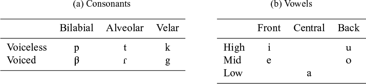
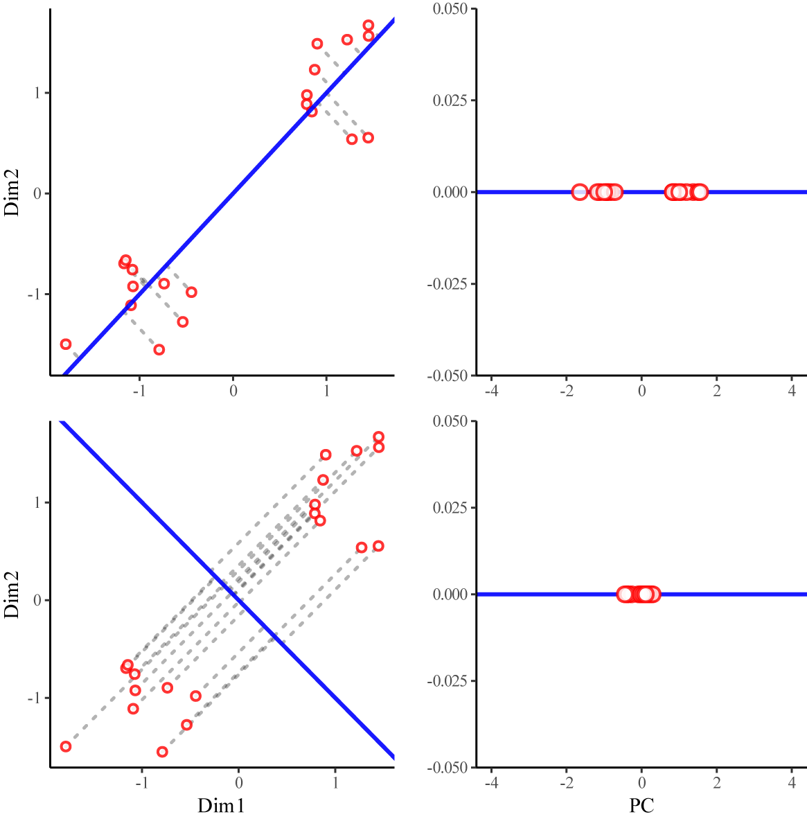


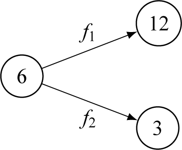
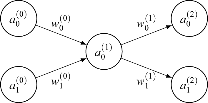


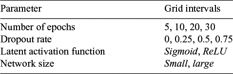


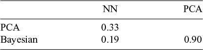


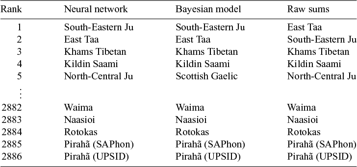
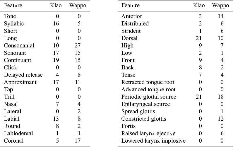


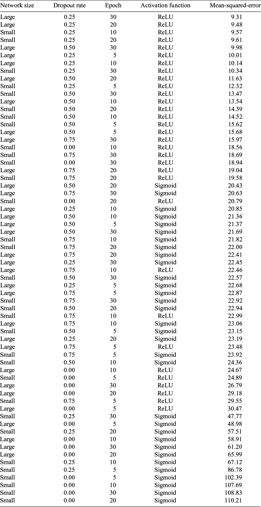

 Open access