Archaeological Background

The LSU Campus Mounds (16EBR6) is a two-mound complex located on the campus of Louisiana State University (LSU). The site is situated on the edge of the Pleistocene terrace overlooking the Mississippi River valley immediately to the west. Each mound is conical, approximately 5.3 m in height and 35–40 m in diameter.

In 1982, three soil cores were obtained from the crest of each mound, and a brief description of the sediments was completed (Neuman Reference Neuman1988). An additional three cores were subsequently recovered from Mound A to obtain datable sediments. Bulk sediment recovered from the pre-mound surface and the basal mound fill produced three dates, which indicated that the mound was built during the Middle Archaic period (cf. McGimsey et al. Reference McGimsey, Saunders, Homburg, Hawkins, McKillop and Mann2022:Table 1).

Limited test excavations were conducted around the mound bases in 1985 in advance of landscaping activities. No artifacts were recovered during the coring or testing at the mounds. Additional analyses of the 1982 cores included particle size, pH, and soil chemistry (Homburg Reference Homburg1988).

In 2009, a geophysical class at LSU conducted ground-penetrating radar (GPR), electrical resistivity, and cesium vapor gradiometry survey of each mound (Ellwood Reference Ellwood2009). The GPR survey of each mound experienced high attenuation (loss) of the signal at shallow depths, likely reflecting the high clay and moisture content of the mound fill. The resistivity and gradiometry surveys identified a large anomaly within Mound A; Mound B exhibited a very uniform character and no anomalies. A soil core was recovered from Mound A to evaluate this anomaly, and a core was also recovered from Mound B for comparative purposes (Mann Reference Mann2009). Each core was sampled for magnetic susceptibility. The Mound A magnetic data identified several deposits with magnetic levels interpreted to be too high for redeposited A horizon sediment and therefore may represent fired surfaces. Mound B did not exhibit similar magnetic variation. A bulk sediment sample from the Mound A core was dated (see Beta in McGimsey et al. Reference McGimsey, Saunders, Homburg, Hawkins, McKillop and Mann2022:Table 1). A test unit was then placed in the mound to further explore the anomaly (Mann Reference Mann2012). The unit did not reveal any evidence of what caused the magnetic anomaly and did not recover any artifacts. The profile did not reveal any evidence of burned surfaces or ash layers, as suggested by the magnetic susceptibility data. In 2018, a test unit was opened on Mound B, but it only penetrated the upper meter due to extremely dry and compact sediments. No artifacts were recovered.

The soil cores and limited test excavations indicate that the two mounds are similar in construction but that they utilized somewhat different sediments. Mound A is characterized primarily by basket-loaded A and E horizon silt loam, whereas Mound B has a much greater frequency of B horizon silty clay sediments. No evidence of intermediate surfaces or paleosols was observed, indicating that each mound was built in a single effort (Homburg Reference Homburg1988). Artifacts are notably absent from the mound fill and in the limited testing around the mound bases. The radiocarbon dates identify the mounds as Middle Archaic in age. They represent one of 14 Middle Archaic mound groups recognized in Louisiana along the Mississippi River valley (Saunders Reference Saunders and Rees2010). The location of the LSU Campus Mounds and the other Middle Archaic mound sites in Louisiana can be seen on the map in McGimsey et alia (Reference McGimsey, Saunders, Homburg, Hawkins, McKillop and Mann2022).

Between 2018 and 2022, Ellwood (at LSU) and colleagues undertook extensive analyses of the cores recovered from Mounds A and B in 2009 (Ellwood et al. Reference Ellwood, Warny, Hackworth, Ellwood, Tomkin, Bentley, Braud and Clayton2022). Their analyses followed up on the magnetic susceptibility results noted above. This analysis identified a series of fired surfaces on which quantities of reed or cane had been burned, particularly in Mound A. Numerous radiometric assays on burned phytoliths recovered from the fired surfaces led them to conclude that mound construction began as early as 11,000 years ago. The dates also suggested a significant hiatus in the construction of each mound around 8,000 years ago, with construction ceasing around 6,000 to 5,000 years ago (Ellwood et al. Reference Ellwood, Warny, Hackworth, Ellwood, Tomkin, Bentley, Braud and Clayton2022). The Ellwood et alia (Reference Ellwood, Warny, Hackworth, Ellwood, Tomkin, Bentley, Braud and Clayton2022) interpretation of the mound age of about 13,000 years is a major reinterpretation of the history of mound building in North America. For a long time, the building of mounds more than 2,500 ago was not accepted. Only in the 1990s was this assumption corrected, when numerous mounds dating to 5000–6000 BP were documented—for example, in Louisiana (Saunders et al. Reference Saunders, Mandel, Saucier, Allen, Hallmark, Johnson and Jackson1997) and in the lower Atlantic and on the Gulf Coast (Russo Reference Russo2008).

In a review of the Ellwood et alia’s article (Reference Ellwood, Warny, Hackworth, Ellwood, Tomkin, Bentley, Braud and Clayton2022), McGimsey et alia (Reference McGimsey, Saunders, Homburg, Hawkins, McKillop and Mann2022) identify a number of issues where there are critical gaps in the data used to derive the hypotheses regarding the mound’s age and construction history. They identified the following six topics where further research would enable better assessment of these hypotheses:

1. 1. Determine densities of phytoliths in sediments associated with cane brakes.

2. 2. Reexamine and/or extract new cores to answer specific questions regarding the presence of paleosols (Neuman’s (Reference Neuman1988) cores were destroyed by flooding in the building in which they were stored).

3. 3. Use independent evidence for firing of the mound sediments.

4. 4. Compare gray bands with E horizons in undisturbed soils in the immediate area.

5. 5. Compare dark bands in Mound A with A horizon sediment in the immediate area.

6. 6. Use optically stimulated luminescence (OSL) dating to provide an independent means for dating the burial of the sediments.

Our article presents a first effort to address one or more aspects raised in Topics 1, 3, 4, and 5. Based on these aspects, we have formulated four hypotheses that were tested using synchrotron radiation–based techniques. These hypotheses will be discussed in some detail in Results and Discussion.

Synchrotron Radiation and the Applied Techniques

In this study, two synchrotron radiation–based X-ray techniques are used to address four of the questions/concerns raised by McGimsey et alia (Reference McGimsey, Saunders, Homburg, Hawkins, McKillop and Mann2022): (1) SR-XRF for determining the elemental concentration of samples and XAS; and especially (2) XANES spectroscopy for determining the chemical state of elements in a sample.

Synchrotron radiation (SR) is the radiation emitted by electrons that are moving at about the speed of light and then are deflected, for example, by a magnetic field. This happens, for instance, in circular accelerators for electrons—that is, betatrons, synchrotrons, or storage rings. Two properties in particular make synchrotron radiation an outstanding source for spectroscopic investigations (for further details, see e.g., Balerna and Mobilio Reference Balerna, Mobilio, Mobilio, Boscherini and Meneghini2015):

1. 1. Synchrotron radiation forms a “continuum”—that is, all wavelengths from the infrared to the hard X-ray range are emitted without any gaps.

2. 2. Synchrotron radiation is brighter than any other source covering a broad wavelength range, such as the sun or a light bulb. In the vacuum ultraviolet and in the X-ray range, synchrotron radiation is by far the most intense radiation source.

In X-ray fluorescence (XRF) spectroscopy experiments, the sample of interest is irradiated by an external X-ray source—here, synchrotron radiation of a defined energy. Electrons from so-called inner shells of an atom (that is, electrons with a high binding energy) are knocked out of their shell and then replaced with electrons from higher shells with a lower binding energy. In this process, atoms in the sample are emitting element-specific X-rays whose energy and intensity are then detected by a suitable detector. In this way, the various elements in a sample can be identified and quantified. Because of its extremely high intensity in the X-ray range, using synchrotron radiation for X-ray fluorescence (SR-XRF) experiments increases the sensitivity for trace elements and improves the detection limits (to the ppm level) in general. Consequently, it significantly reduces the quantity of sample material that is required for the experiments. In addition, XRF is an almost nondestructive technique—a property of great importance, specifically for valuable archaeological artifacts.

XAS is a spectroscopic technique for the element-specific geometric, chemical, and electronic characterization of materials on an atomic scale. When measuring the XAFS (X-ray absorption fine structure), tunable monochromatic X-rays (as provided by monochromatized synchrotron radiation) are used for measuring the energy dependence of the photoabsorption coefficient μ(E) in a narrow region around an inner shell absorption energy of the element of interest, visible as a jump of the absorption coefficient when the energy of the incoming photon is high enough to excite the corresponding inner shell electrons into an empty outer shell or into the continuum. In general, this jump in the absorption coefficient is called “edge.”

The XAFS spectrum is divided into two parts: (1) the X-ray absorption near edge structure (XANES), which starts approximately 50 eV before the “edge” and reaches up to roughly 50–100 eV above the edge; and (2) the extended X-ray absorption fine structure (EXAFS), which is visible up to about 1,000 eV above the edge. EXAFS contains element-specific geometric and chemical information: number, type, and distance of neighboring atoms. In this project, only XANES was used. XANES contains detailed information about the electronic structure of the local vicinity of the absorbing atom species (Bunker Reference Bunker2010; Calvin Reference Calvin2013). Consequently, the energy position and shape of the absorption edge depend sensitively on the chemical environment of the absorbing atom. Compared to X-ray diffraction, XAFS does not require long-range order (i.e., crystallinity of the sample), so it can also be applied to amorphous materials (e.g., glass or rubber). As a result, XAFS provides information about the crystalline and the noncrystalline parts of samples. This makes the direct comparison with X-ray diffraction data as they exist for the LSU mounds rather problematic, in particular because samples have a high content of silt with grain sizes too small for X-ray diffraction (XRD) measurement (Homburg Reference Homburg1988). Compared to most other techniques providing similar information, XAFS has some additional advantages: it is nondestructive, element-specific, and extremely sensitive; material does not need to be taken material out of a sample; and samples do not need to be “prepared.” The theoretical basics of XAFS, the various techniques used with it for measuring and for data reduction, and its broad range of applications are discussed in numerous textbooks, review articles, and conference proceedings (Bunker Reference Bunker2010; Calvin Reference Calvin2013; Kozak et al. Reference Kozak, Kwiatek, Kiskinova, Augusto and Sakura2020; Newville Reference Newville, Henderson, Neuville and Downs2015).

For archaeological materials, analysis of the chemical state of suitable elements using XAFS spectroscopy and, specifically, XANES can provide information about details of the manufacturing process, aging processes, and occasionally also the utilization of an artifact (Cotte et al. Reference Cotte, Susini, Dik and Janssens2010; Janssens and Cotte Reference Janssens, Cotte, Jaeschke, Khan, Schneider and Hastings2020).

Experimental Details and Investigated Samples

For the experiments described here, five samples from a total of 18 available soil samples of the core drilled in 2009 from Mound B are investigated. Access to these samples was kindly provided by Prof. Brooks Ellwood. The samples are summarized in Table 1 together with the depth of their location in the mound (the top of the mound is defined as depth “0 m”), their specific meaning for this investigation, and the experiments performed with that sample. Based on the available samples and the experiments suggested by McGimsey et alia (Reference McGimsey, Saunders, Homburg, Hawkins, McKillop and Mann2022) that have been discussed before, two groups of samples were compared:

1. 1. LSU 10 ↔ LSU 11: these are samples from the two hypothesized building periods of the mounds, roughly 2,000 years apart. LSU 10 is from a depth of 3.45 m (that is, from the upper part of the mound built in phase 1), and LSU 11 is from a depth of 2.65 m and therefore from the first layers of the second building phase (Ellwood et al. Reference Ellwood, Warny, Hackworth, Ellwood, Tomkin, Bentley, Braud and Clayton2022).

2. 2. LSU 6 ↔ LSU 5 ↔ LSU 7: LSU 5 is from a light-colored lens (depth of 5.36 m), LSU 6 is from just below (depth of 5.52 m), and LSU 7 is from just above LSU 5 (depth of 5.20 m; see explanations in Table 1). Figure 1 depicts a small part of the core from Mound B. The left side shows the lighter material (called ash lens by Ellwood et al. Reference Ellwood, Warny, Hackworth, Ellwood, Tomkin, Bentley, Braud and Clayton2022), and the right side shows the darker material (soil) just above the ash lens.

Table 1.

The Investigated Samples of Mound B.

^a The depth of the sample relative to the top of Mound B that has depth 0.

^b XRF-HE = SR-XRF with 13.9 keV excitation energy.

^c XRF-LE = SR-XRF with 4.5 keV excitation energy.

^d Elements and edges that have been measured using XANES.

^e These year dates were provided by Brooks Ellwood. Remarks = Characteristic properties of the samples.

Figure 1.

A photo of a small part of the core of Mound B. The left side shows the lighter material (ash lens?), and the right side shows the normal, darker soil just above the light material. (Color online)

For this study, each sample was ground in an agate mortar and then spread very thinly on the adhesive side of a suitable polymer tape for limiting the dead-time of the X-ray fluorescence detector below 10%.

Experiments were carried out at the ASTRA beamline at the SOLARIS storage ring (Kraków, Poland; Hormes et al. Reference Hormes, Klysubun, Göttert, Lichtenberg, Maximenko, Morris and Nita2021) and at the DCM beamline at the Louisiana State University Center for Advanced Microstructures and Devices (LSU-CAMD; Roy et al. Reference Roy, Morikawa, Bellamy, Kumar, Göttert, Suller, Morris, Kurtz and Scott2011). At both facilities, a modified vacuum double crystal X-ray monochromator (Lemonnier et al. Reference Lemonnier, Collet, Depautex, Esteva and Raoux1978) was used for monochromatizing the X-rays, and a single-element silicon drift detector was used for detecting the fluorescence radiation. For higher X-ray energies (e.g., the XRF excitation at 13.9 keV), germanium (Ge; 220) crystals were used, and for the low energy range (below ∼5 keV), indium antimonide (InSb; 111) crystals were employed. The incoming intensity I₀ was monitored using an ionization chamber. The SOLARIS storage ring operated at an electron energy of 1.5 GeV at currents between 400 mA and approximately 200 mA, whereas the LSU-CAMD storage ring operated at 1.1 GeV at currents between 150 mA and roughly 50 mA.

X-ray fluorescence experiments were conducted at two excitation energies: 13.9 keV for high-Z elements (higher than Z = 18 [Ar]) with samples in air, and 4.5 keV for low-Z elements, either with reduced pressure of approximately 15 Torr or with vacuum in the sample chamber. Integration time for all SR-XRF measurements was 15 minutes per spectrum. Detailed (semi-)quantitative analysis of XRF spectra was carried out using the PyMca program (Solé et al. Reference Solé, Papillon, Cotte, Walter and Susini2007).

XANES spectra have been recorded for two elements: silicon (Si) and iron (Fe). Si was chosen because it is the “central element” in phytoliths (Strömberg et al. Reference Strömberg, Dunn, Crifò, Harris, Croft, Su and Simpson2018). Phytoliths are rigid, microscopic structures made of silica (SiO₂) that are found in all plants and that persist after the decay of the plant; for example, by burning the plants. Plants take up silica from the soil along with their nutrients and water. As reported by Ellwood et alia (Reference Ellwood, Warny, Hackworth, Ellwood, Tomkin, Bentley, Braud and Clayton2022), “huge concentrations” of burned reed and cane-plant phytolith residues were found in the light-colored areas of both mounds. For the assignment of phytoliths to specific plants (here, reed and cane), morphology was used although a specific plant can have a great number of morphotypes as was shown, for example, by Chowdhary et alia (Reference Chowdhary, Badgal, Bhat, Shakoor, Mir and Soodan2023). Chowdhary and colleagues (Reference Chowdhary, Badgal, Bhat, Shakoor, Mir and Soodan2023) studied phytoliths also using X-ray diffraction, and they found a mixture of several forms of silica, such as cristobalite, tridymite, quartz, zeolite, and other forms. To the best of our knowledge, no XAFS measurements of phytoliths are reported in the literature. For the measurements at the Si-K edge, the energy was calibrated to the maximum of the white line of amorphous SiO₂ (diatomite) at 1846.9 eV.

Fe is one of the heat-sensitive elements that, in a suitable matrix, changes its chemical environment when heated to high temperatures in an oxidative (air) or reductive atmosphere. This was shown, for example, by the various experiments and measurements of Matsunaga and Nakai (Reference Matsunaga and Nakai2004) when using Fe-K-XANES spectra for studying the firing technique of pottery from Kaman-Kalehöyük, an archaeological site in Turkey. For the measurements at the Fe-K edge, energy of the monochromator was calibrated by setting the first turning point in the XANES spectrum of a Fe-metal foil to 7112 eV. XANES data were normalized and analyzed using the ATHENA program of the IFEFFIT package (Ravel and Newville Reference Ravel and Newville2005).

To check the reproducibility of the spectra (for both XRF and XANES measurements), each measurement was carried out at least twice, and in many cases, also on different days and by using newly prepared samples.

Results and Discussion

Based on the suggestions from McGimsey et alia (Reference McGimsey, Saunders, Homburg, Hawkins, McKillop and Mann2022), for additional experiments, we formulated four hypotheses as starting points of our research. In this section, our results are discussed in the framework of the corresponding hypothesis, with the goal of finding either agreement with or disagreement with the hypothesis.

Hypothesis 1

Soils used at least several hundred years apart for building Mound B will have a different elemental composition, assuming that they were obtained from different source areas. However, even when coming from the same “source,” soils should have a different composition due to modification caused by the five factors that soil scientists deem responsible for the formation and variations of soil: parent material, climate, biota (organisms), topography, and time (Sposito Reference Sposito2008; University of Minnesota Extension 2018). The influence of climate (temperature and precipitation)—the parameter that strongly influences changes in the elemental composition of a soil, mainly by chemical weathering—is discussed by, for example, Abbaslou et alia (Reference Abbaslou, Abtahi and Baghernejad2013), Sposito (Reference Sposito2008), Ouimet (Reference Ouimet2008), Homburg (Reference Homburg1988), and references provided in these publications.

This hypothesis is tested using group 1 samples (see previous section). The basis for this hypothesis is the assumption that the elemental composition of a material—and here, specifically the trace elements—is a distinct “fingerprint” of the point of origin of that material. This assumption has been confirmed by numerous measurements of natural materials, such as stones and sands in other contexts (Cullers Reference Cullers2002; Finlay et al. Reference Finlay, McComish, Ottley, Bates and Selby2012; Poretti et al. Reference Poretti, Brilli, De Vito, Conte, Borghi, Günther and Zanetti2017).

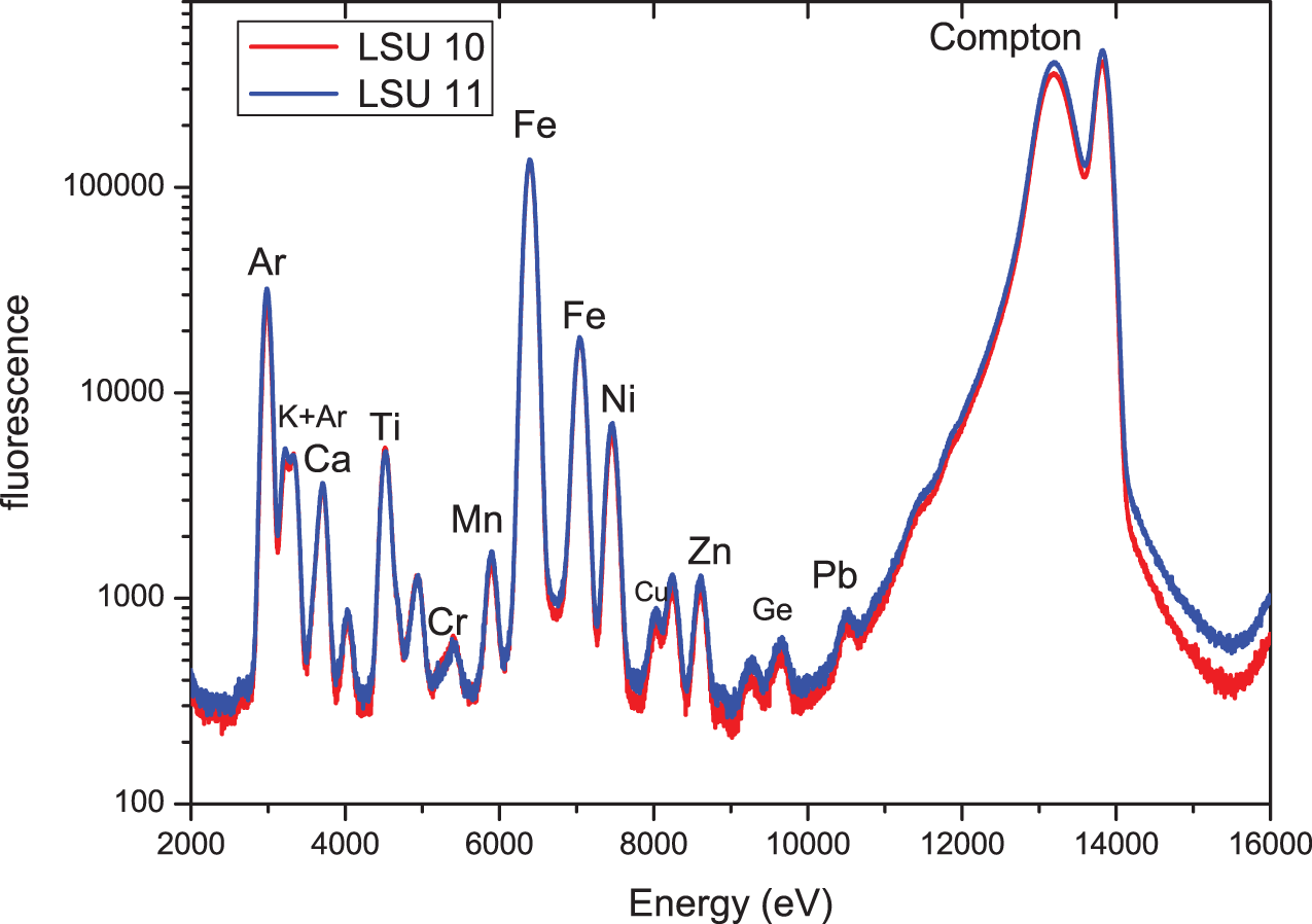
Figure 2 shows the X-ray fluorescence spectra of samples LSU 10 and LSU 11 with an excitation energy of approximately 13.9 keV (samples in air). XRF spectra are plotted on a logarithmic scale so that trace elements are also visible. For a comparison of intensities and the element concentrations, the spectra are normalized to the Compton peak. Alternatively, analysis demonstrated that normalizing the spectra to the intensity of the argon (Ar) fluorescence peak produced identical results. The Ar fluorescence does not come from the samples but from the air “around” the sample. Therefore, the concentration of Ar is constant for all measured samples. In Figure 3, the easily visible peaks are assigned to 12 identified corresponding elements. For this figure and for Figures 4, 5, and 6, all fluorescence lines for elements up Ge (Z = 32) are K_α-lines—that is, an electron from the K-shell with the highest binding energy knocked out by the exciting X-rays and electrons from the neighboring L-shell filling the hole. Given that the L-shell has two subshells with different energies, there are always two fluorescence lines, K_α1 and K_α2. However, because of the lower intensity of the high energy K_α2-line, this is only directly visible for elements with high concentration (in Figure 2, for example, Fe). For lead (Pb), one sees a L_β-line—that is, a hole in the L-shell filled up by electrons from the M-shell. There are no significant differences between the spectra of the two samples. However, such a coarse analysis does not take into account that sometimes fluorescence peaks from various elements overlap (mainly due to the “bad” energy resolution of standard X-ray fluorescence detectors of about 150 eV), and there are some lines that can be assigned to the interaction of the fluorescence photons with the (Si-) detection chip of the detector (e.g., escape peaks). Moreover, this type of first-step analysis does not provide any (semi-)quantitative results. To overcome these problems, the spectra are fit using a suitable analysis software, such as PyMca (Solé et al. Reference Solé, Papillon, Cotte, Walter and Susini2007). Based on the well-known absorption and emission coefficients for all elements and a specific set of properties of the setup used for the data collection, this program fits the measured spectra and provides (semi-)quantitative results for the element concentration in the measured samples.

Figure 2.

SR-XRF spectra of LSU 10 and LSU 11; excitation energy 13.9 keV; measurements in air. (Color online)

Figure 3.

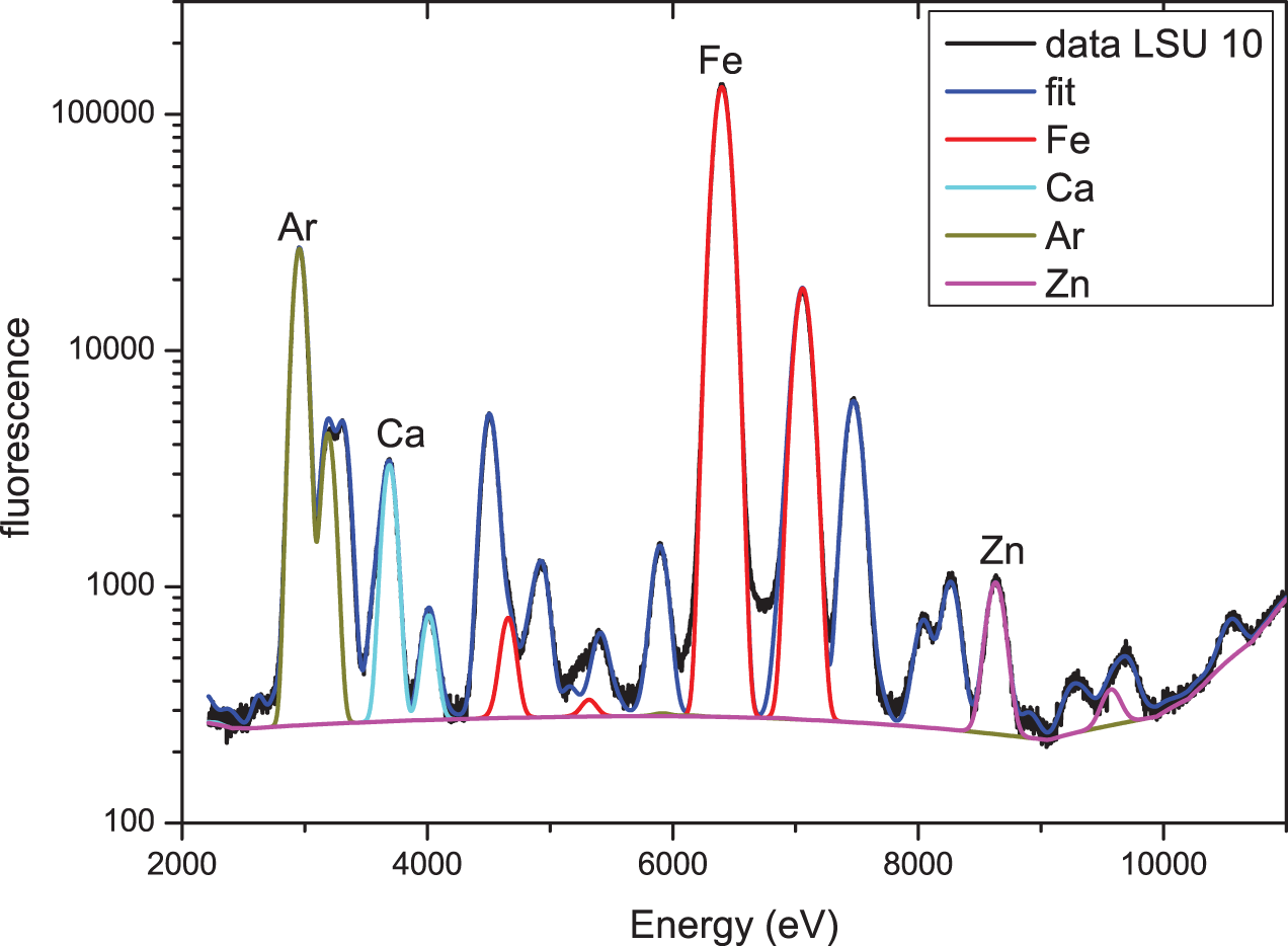
SR-XRF spectrum of LSU 10 (excitation energy 13.9 keV) together with the corresponding PyMca fit and the contributions of four selected elements (Ar, Ca, Fe, Zn) to this fit. (Color online)

Figure 4.

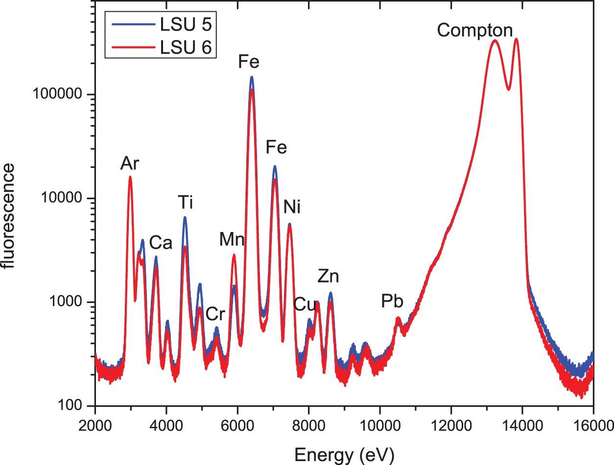
SR-XRF spectra of LSU 5 and LSU 6; excitation energy 13.9 keV; measurements in air. (Color online)

Figure 5.

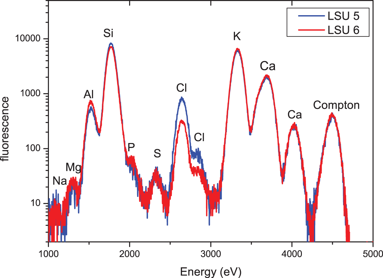
SR-XRF spectra of LSU 5 and LSU 6; excitation energy 4.5 keV; samples in vacuum. (Color online)

Figure 3 shows the measured SR-XRF spectrum of LSU 10 together with the fit obtained by using PyMca and the contribution to this fit from four selected elements (Ar, Ca, Fe, Zn). Specifically, the contribution from Fe shows quite clearly that not just the characteristic fluorescence (Fe – K_α1 at ∼6,405 eV) but also the so-called escape peak (here at ∼4,666 eV, i.e., energy Fe K_α1 – energy Si K_α1) contributes to the fit. The fit, using 18 elements, is quite good, and the concentrations derived from this fit for LSU 10 and LSU 11 agree quite well within the error bars for the concentration. This result strongly supports the statement already derived from Figure 2 that there are no significant differences in the elemental distribution of the two samples.

Hypothesis 2

Samples from the light-colored areas—that is, possibly ash—should have a significantly different elemental composition compared to soil samples from the “darker” areas, because ash and soil are basically different materials.

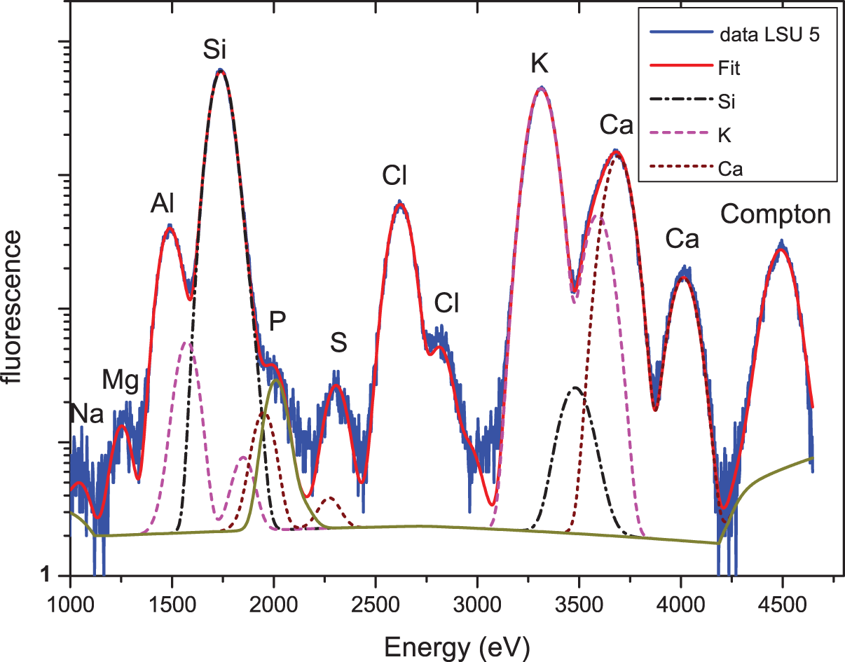
This hypothesis is tested by the samples of group 2, with one sample from a light area (LSU 5) and a sample from just below the light-colored area (LSU 6), which is darker in color. Figure 4 shows the XRF spectra of samples LSU 5 and LSU 6 recorded at an excitation energy of 13.9 keV. For these measurements, samples are again in air so that—due to the very low absorption of air—Z elements (Z < 18 [Ar]) are not detectable. As in Figure 2, in an initial approach, the stronger fluorescence peaks are assigned to the corresponding elements. It is obvious that there are no significant differences between the two spectra in Figure 4. However, because Ellwood et alia (Reference Ellwood, Warny, Hackworth, Ellwood, Tomkin, Bentley, Braud and Clayton2022) report a very high concentration of phytoliths and therefore a high concentration of Si in the light-colored areas, the low energy excitation XRF spectra (excitation energy 4.5 keV, samples in vacuum) of the two samples were also measured. These spectra are shown in Figure 5. Again, the stronger peaks are assigned to the corresponding elements. It is again apparent that there are no significant differences in the elemental concentration of samples LSU 5 and LSU 6.

Figure 6.

SR-XRF spectrum of LSU 5 (excitation energy 4.5 keV) together with the corresponding PyMca fit and the contributions of three selected elements (Si, K, Ca) to this fit. (Color online)

For verification of the assignment of elements and for a more quantitative analysis of the spectra, spectra were again fitted using the PyMca program. The results of the fit of sample LSU 5 is shown in Figure 6, with the contribution of some selected elements (Si, K, Ca). Similar to the results described in Hypothesis 1, this advanced analysis did not show any significant differences between the elemental concentrations of the two samples. However, there are at least three remarkable features in the low-energy XRF spectra that require further investigation. The first is the rather high concentration of K as compared to Ca. The second is the rather high concentration of Cl, and the third is the extremely low concentration of phosphorus.

Hypothesis 3

If the light areas consist mainly of phytoliths, or if the concentration of phytoliths is just very high (Ellwood et al. Reference Ellwood, Warny, Hackworth, Ellwood, Tomkin, Bentley, Braud and Clayton2022), Si-K-XANES spectra that are characteristic of the chemical environment of Si should be different for LSU 5 and a sample from the dark-colored soil—for example, LSU 7—where one would expect Si to be in quartz particles and/or in corresponding soil minerals. The basis for this hypothesis is the well-known high sensitivity to the chemical environment of XANES spectra in general and for Si in particular. Dien Li et alia (Reference Li, Bancroft, Fleet and Feng1995) and Jiaqi Li et alia (Reference Li, Zhang, Garbev and Monteiro2021) and the numerous references given in these publications demonstrated this sensitivity by measuring a broad range of Si-containing compounds.

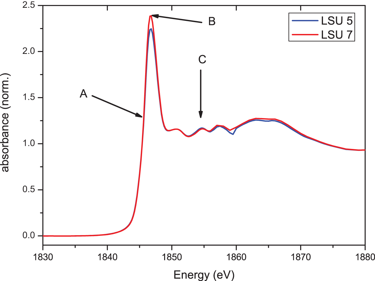
Figure 7 shows the Si-K-XANES spectra of LSU 5 (from a light area) and LSU 7 (from a dark area just above LSU 5). The spectra show no significant differences regarding their characteristic spectral features, marked with arrows in Figure 7: (A) the energetic position of the rise to the white line, (B) the energy position of the white line (first maximum after the edge), and (C) the fine structure on the high-energy side of the white line. These agreements show that the Si in both samples has the identical chemical environment; the small difference in the amplitude of the white line can be regarded as not significant, given that this is within the error margins caused by the measurements themselves but mainly by the data reduction (background subtraction, etc.).

Figure 7.

Si-K-XANES spectra of LSU 5 and LSU 7; characteristic spectral features are marked with arrows and letters: (A) energetic position of the rising edge to the white line, (B) energy position of the white line, and (C) fine structure on the high-energy side of the white line. (Color online)

Remarkably, the pronounced fine-structure C on the high-energy side of the white line (above ∼1,850 eV, called “shape resonances”) indicates that the Si in both samples exists mainly in a crystalline environment. There are three well-resolved structures that resemble those seen in crystalline SiO₂ (quartz). However, given that the intensity ratios are very different from those in quartz, quartz can be ruled out as the dominant chemical form of Si in the samples. As far as we know, none of the minerals and other chemical forms of Si that have been investigated until now show this distinct triplet of lines. It is possible that Si exists in various crystalline forms and that the measured spectrum is an overlap of the corresponding spectra or—which seems more unlikely—that Si exists in a form that has not yet been identified and measured using XAS.

Hypothesis 4

There are several “heat sensitive elements” (e.g., Ca and Fe) that change their chemical environment (or more simply, change their valency) when heated to high temperatures in an oxidative (air) and/or reductive environment. Consequently, the corresponding XANES spectra of corresponding elements from the light areas (ash) heated to very high temperature, according to Ellwood et alia (Reference Ellwood, Warny, Hackworth, Ellwood, Tomkin, Bentley, Braud and Clayton2022) should be different from those of the dark areas. For Fe, this behavior was documented by Matsunaga and Nakai (Reference Matsunaga and Nakai2004). For Ca, this behavior was analyzed in more detail by Hormes et alia (Reference Hormes, Bovenkamp-Langlois, Klysubun and Kizilkaya2020), who showed that it is actually possible to derive absolute firing temperatures of ceramics from these XANES spectra when suitable reference spectra are available.

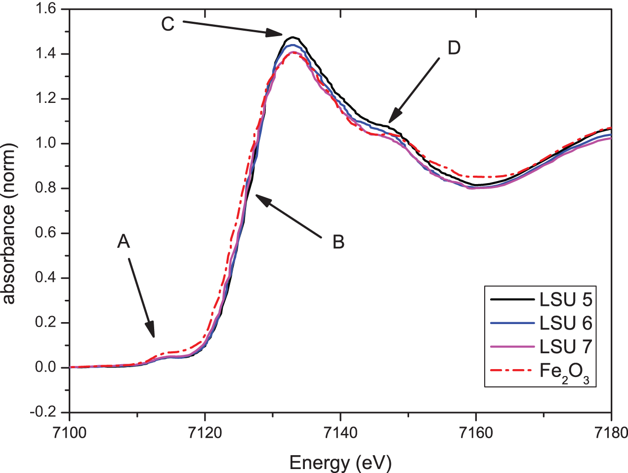
Figure 8 shows the Fe-K-XANES spectra of LSU 5—the sample from a light-colored lens—in comparison with the corresponding spectra of LSU 6 and LSU 7 samples from just below and above LSU 5. For comparison, the Fe-K-XANES spectrum of Fe₂O₃ is also shown. Marked by arrows and letters are the characteristic features of the spectra: (A) a pre-edge structure, (B) the rising edge to the white line, (C) the maximum of the white line, and (D) the pronounced shoulder on the high-energy side of the white line. The three spectra of the LSU mound samples have an identical pre-edge structure, the same energy for the rising edge, and the same energy position of the white line. The energy position of the “rising edge” B indicates that Fe in all three samples has the formal valency +3. The minor deviations regarding the intensity of the white line and the intensity of the shoulder D cannot be regarded as significant. In summary, Fe is in all three samples in the identical chemical environment, and there are no differences between the light-colored area and the dark-colored areas. This is strong evidence against the assumption that the “material” in sample LSU 5 was heated to a very high temperature. Compared to the XANES spectrum of Fe₂O₃, the spectra of the mound samples show some small deviations: the pre-edge feature A is less pronounced, the rising edge B of Fe₂O₃ is lower in energy than for the mound samples, and the high-energy shoulder D is shifted to higher energies compared to the mound samples. These differences show that the Fe in the mound samples does not exist purely as Fe₂O₃ but either in a different chemical environment or as a mixture between Fe₂O₃ and a Fe-containing compound with the formal valency +3 but with a stronger electronegativity than oxygen. To clarify these questions, further analyses with additional reference samples are necessary.

Figure 8.

Fe-K-XANES spectra of LSU 5, LSU 6, LSU 7, and Fe₂O₃ as a reference spectrum. The characteristic features of the spectra are marked by arrows and letters: (A) the pre-edge structure, (B) the rising edge to the white line, (C) the maximum of the white line, and (D) the pronounced shoulder on the high-energy side of the white line. (Color online)

Conclusions and Further Investigations

The results of this investigation show quite clearly the usefulness of the applied SR-based techniques for the investigation of soil samples of archaeological relevance. The results contradict all four hypotheses and therefore support neither the assumption that Mound B was built in two phases with a hiatus of approximately 1,000 to 2,000 years nor the assumption that the light-colored lenses consist of ash from hot fires.

The next phase of our investigation will include the following:

• • XRF measurements of the other available samples (specifically those from other light areas) will be undertaken.

• • XANES spectra will be recorded of additional relevant elements (e.g., P and S) to examine the question of where the obvious color differences between the light areas and the dark soil come from.

• • Additional drilling will be carried out near the mounds and at other appropriate places for obtaining suitable soil reference samples to address the question of where the soil for building the mounds came from.